Combining Textural Descriptors forForest Species Recognition

J. G. MartinsTechnological Federal University of Parana

R. Cristo Rei, 19,Toledo, PR, Brasil - 85902-490

Email: martins@utfpr.edu.br

L. S. OliveiraFederal University of Parana

R. Cel. Francisco H. dos Santos, 100,Curitiba, PR, Brazil - 81531-990

Email: lesoliveira@inf.ufpr.br

R. SabourinEcole de Technologie Superieure

1100 rue Notre Dame Ouest,Montreal, Quebec, Canada

Email: robert.sabourin@etsmtl.ca

Abstract—In this work we assess the recently introducedLocal Phase Quantization (LPQ) as textural descriptor for theproblem of forest species recognition. LPQ is based on quantizingthe Fourier transform phase in local neighborhoods and thephase can be shown to be a blur invariant property undercertain commonly fulfilled conditions. We show through a seriesof comprehensive experiments that LPQ surpasses the resultsachieved by the widely used Local Binary Patterns (LPB) andits variants. Our experiments also show, though, that the resultscan be further improved by combining both LPB and LPQ. Inthis sense, several different combination strategies were triedout. Using a SVM classifiers, the combination of LPB and LPQbrought an improvement of about 7 percentage points on adatabase composed by 2,240 microscopic images extracted from112 different forest species.

I. INTRODUCTION

The field of wood Anatomy has defined a set of primitivesto discriminate the vegetable species from which wood canbe extracted. Besides the scientific importance, wood identifi-cation has a huge practical importance. Wood is a basic rawmaterial applied to make a plenty of products. So, woods canalso be categorized by their different applications accordingto their physical, chemical, and anatomical characteristics, andtheir prices vary greatly.

Large quantities of wood are transported among short orlong distances all over the world. The safe trade of log andtimber has become an important issue. Buyers must certifythey are buying the correct material while supervising agencieshave to certify that wood has been not extracted irregularlyfrom forests. This matter involves millions of dollars and aimsat preventing frauds where a wood trader might mix a noblespecies with cheaper ones, or even try to export wood whosespecies is endangered.

Nowadays, timber is examined by using the naked eyeor sometimes with the aid of a magnifier. In addition tothe macroscopic features of wood, physical features such asweight (different moisture content), color (variation), feel,odour, hardness, texture, and surface appearance are also con-sidered. However, identifying an wood log or timber outsideof its context (the forest) is not an easy task since onecannot count on flowers, fruits, and leaves. Therefore thistask is performed by well-trained specialists but few reachgood accuracy in classification due to the time it takes for

their training, hence they are not enough to meet the industrydemands. Another factor to be taken into account is that theprocess of manual identification is rather subjective and timeconsuming. It might lead to diversion of attention as it is arepetitive process and consequently may result in errors, whichcan become impracticable when checking cargo for export. Inthis context, computer vision systems become very interesting.In the last decade, however, most of the applications ofcomputer vision in the wood industry were related to qualitycontrol, grading, and defect detection [1], [2].

Just recently, some authors began to use computer vision toclassify forest species. Tou et al [3] reported two experimentsto classify forest species which also use the gray-level co-occurrence matrix (GLCM) features to train a neural networkclassifier. The authors report recognition rates ranging from60% to 72% for five different forest species.

Khalid et al [4] presented a system to recognize 20 differentMalaysian forest species. A particularity of this method isthat the wood samples were first boiled and then cut witha microtome into thin sections. The image acquisition wasthen performed with an industrial camera of high performanceand a LED array lighting. The recognition process is basedon a neural network trained with information extracted fromGLCM. The database used in their experiments contains 1,753images for training and only 196 for testing. They report arecognition rate of 95%. A drawback of this strategy is theexpensive acquisition protocol which makes it unfeasible forreal applications.

Paula et al [5] investigated the use of GLCM and color-based features to recognized 22 different species of the Brazil-ian flora. In this work they have proposed a segmentation strat-egy to deal with the great intra-class variability. Experimentalresults show that when color and GLCM features are usedtogether the results can be considerably improved.

In this work we assess the Local Phase Quantization (LPQ)as textural descriptor for the problem of forest species recogni-tion. LPQ is based on quantizing the Fourier transform phasein local neighborhoods and the phase can be shown to bea blur invariant property under certain commonly fulfilledconditions. Our experiments were performed on a recentlyproposed database composed of 2,240 microscopic imagesfrom 112 different forest species [6]. Such a database is

available for research purposes under request1.A series of comprehensive experiments show that the LPQ

surpasses the results achieved by the Local Binary Patterns(LPB) and its variants (LBPu28,2, LBPri8,2, LBPriu28,2 ). In spite ofthat, we show that the LPQ results can be further improved bycombining them with LPB. In this vein, several different com-bination strategies were tried out along with a SVM classifier.The best results were achieved by fusing the results of the LPQand LPBri8,2 with the Product rule. Such a combination broughtan improvement of about 7.1 percentage points compared tothe best results reported in [6].

This paper is structured as follows: Section II introducesthe used image database. Section III describes the featuresets we have used to train the classifiers. Section IV reportsour experiments and discusses our results. Finally, section Vconcludes the work.

II. DATABASE

The database used in this work contains 112 differ-ent forest species which were catalogued by the Labo-ratory of Wood Anatomy at the Federal University ofParana in Curitiba, Brazil [6]. As stated before, it is avail-able for research purposes upon request to the VRI-UFPR(http://web.inf.ufpr.br/vri/forest-species-database). The proto-col adopted to acquire the images comprises five steps. Inthe first step, the wood is boiled to make it softer. Then, thewood sample is cut with a sliding microtome to a thickness ofabout 25 microns (1 micron = 1× 10−6 meters). In the thirdstep, the veneer is colored using the triple staining technique,which uses acridine red, chrysoidine, and astra blue. In thefourth step, the sample is dehydrated in an ascending alcoholseries. Finally, the images are acquired from the sheets ofwood using an Olympus Cx40 microscope with a 100x zoom.The resulting images are then saved in PNG (Portable NetworkGraphics) format with a resolution of 1024×768 pixels.

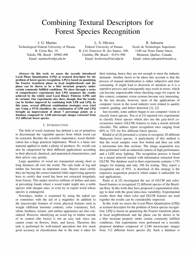
Each specie has 20 images, totalizing 2,240 microscopicimages. Of the 112 available species, 37 are Softwoods and75 are Hardwoods (Fig. 1). Looking at these samples, we cansee that they have different structures. Softwoods have a morehomogeneous texture and/or present smaller holes, known asresiniferous channels (Figure 1a), whereas Hardwoods usuallypresent some large holes, known as vessels (Fig. 1b).

Another visual characteristic of the Softwood species is thegrowth ring, which is defined as the difference in the thicknessof the cell walls resulting from the annual development ofthe tree. We can see this feature in Figure 1a. The coarsecells at the bottom and top of the image indicate moreintense physiological activity during spring and summer. Thesmaller cells in the middle of the image (highlighted in lightred) represent the minimum physiological activity that occursduring autumn and winter.

It is worth noting that color cannot be used as an identifyingfeature in this database, since its hue depends on the dyeingsubstance used to produce contrast in the microscopic images.

1http://web.inf.ufpr.br/vri/forest-species-database

(a) (b)

Figure 1. Samples of the database (a) Softwoods and (b) Hardwoods.

All the images were therefore converted to gray scale (256levels) in our experiments.

III. FEATURES

In order to make this paper self-contained, in this sectionwe briefly describe both textural descriptors assessed in ourexperiments, the Local Phase Quantization and Local BinaryPatterns.

A. Local Phase Quantization (LPQ)

Proposed by Ojansivu e Heikkila [7], LPQ is based onquantized phase information of the Discrete Fourier Transform(DFT). It uses the local phase information extracted using the2-D DFT or, more precisely, a Short-Term Fourier Transform(STFT) computed over a rectangular M×M neighborhood Nxat each pixel position x of the image f(x) defined by

F (u, x) =∑

y∈Nx

f(x− y)e−j2πuT y = wTu fx (1)

where wu is the basis vector of the 2-D DFT at frequencyu, and fx is another vector containing all M2 image samplesfrom Nx.

The STFT can be implemented using a 2-D convolutionsf(x)e−2πju

T x for all u. In LPQ only four complex coefficientsare considered, corresponding to 2-D frequencies u1 = [a, 0]T ,u2 = [0, a]T , u3 = [a, a]T , and u4 = [a,−a]T , where a isa scalar frequency below the first zero crossing of the DFTH(u). H(u) is DFT of the point spread function of the blur,and u is a vector of coordinates [u, v]T . More details about theLPQ formal definition can be found in [7], where Ojansivu eHeikkila introduced all mathematical formalism. At the end,we will have an 8-position resulting vector Gx for each pixelin the original image. These vectors Gx are quantized usinga simple scalar quantizer (Eq. 2, and 3), where gj is the jthcomponent of Gx [7].

qj =

{1, if gj>00, otherwise (2)

b =

8∑j=1

qj2j−1. (3)

The quantized coefficients are represented as integer valuesbetween 0-255 using binary coding (Eq. 3). These binary codes

will be generated and accumulated in a 256-bin histogram,similar to the LBP method [8]. The accumulated values in thehistogram will be used as the LPQ 256-dimensional featurevector.

Codes produced by the LPQ operator are insensitive to cen-trally symmetric blur, which includes motion, out of focus, andatmospheric turbulence blur [9]. Although this ideal invarianceis not completely achieved due to the finite window size, themethod is still highly insensitive to blur. Because only phaseinformation is used, the method is also invariant to uniformillumination changes [7].

B. Local Binary Patterns (LBP)

The original LBP proposed by Ojala et al. [10] labels thepixels of an image by thresholding a 3 × 3 neighborhood ofeach pixel with the center value. Then, considering the resultsas a binary number and the 256-bin histogram of the LBPlabels computed over a region, they used this LBP as a texturedescriptor. Figure 2 illustrates this process.

Figure 2. The original LBP operator.

The limitation of the basic LBP operator is its small neigh-borhood, which cannot absorb the dominant features in large-scale structures. To overcome this problem, the operator wasextended to cope with larger neighborhoods. By using circularneighborhoods and bilinearly interpolating the pixel values,any radius and any number of pixels in the neighborhoodare allowed. Figure 3 depicts the extended LBP operator,where (P,R) stands for a neighborhood of P equally spacedsampling points on a circle of radius R, which forms aneighbor set that is symmetrical in a circular fashion.

Figure 3. The extended LBP operator [11].

The LPB operator LBPP,R produces 2P different binarypatterns that can be formed by the P pixels in the neighbor set.However, certain bins contain more information than others,and so, it is possible to use only a subset of the 2P LBPs.Those fundamental patterns are known as uniform patterns.A LBP is called uniform if it contains at most two bitwisetransitions from 0 to 1 or vice versa when the binary string isconsidered circular. For example, 00000000, 001110000 and11100001 are uniform patterns. It is observed that uniform

patterns account for nearly 90% of all patterns in the (8,1)neighborhood and for about 70% of all patterns in the (16, 2)neighborhood in texture images [10][8].

Accumulating the patterns that have more than two tran-sitions into a single bin yields an LBP operator, denotedLBPu2P,R, with fewer than 2P bins. For example, the number oflabels for a neighborhood of 8 pixels is 256 for the standardLBP but 59 for LBPu2. Then, a histogram of the frequencyof the different labels produced by the LBP operator can bebuilt [10].

LBP variants were proposed in [8]. LBPri and LBPriu2

have the same LBPP,R definition, but they have only 36 and10 patterns, respectively. LBPri accumulates, in only one bin(Eq. 4), all binary patterns which keep the same minimumdecimal value LBP riP,R when their P bits are rotated (ROR).LBPriu2 combines LBPu2 and LBPri definition. Thus, it usesonly the uniform binary patterns and accumulates, in only onebin, those that keep the same minimum decimal value LBP riP,Rwhen their P bits are rotated.

LBP riP,R = min{ROR(LBPP,R, i) i = 0, ..., P − 1}. (4)

IV. EXPERIMENTS AND DISCUSSION

The classifier used in this work was the Support VectorMachine (SVM) introduced by Vapnik in [12]. Normalizationwas performed by linearly scaling each attribute to the range[-1,+1]. The Gaussian kernel was used, with parameters C andtuned using a grid search.

In our experiments, the database was divided into training(40%), validation (20%), and testing (40%). In order to showthat the choice of the images used in each subset doesnot have a significant impact on the recognition rate, eachexperiment was performed five times with different subsets(randomly selected) for training, validation, and testing. Thesmall standard deviation (σ) values show that the choice ofthe images for each dataset is not an important issue.

To analyze the data into a multi-class problem, we used theone-against-others strategy, which works by constructing anSVM ωi for each class q that first separates the class from allthe other classes and then uses an expert F to arbitrate betweentheir SVM outputs, in order to produce the final decision. Agood reference work listing the multi-class SVM methods is[13].

We used estimation of probabilities to proceed the com-bination of outputs in order to get a final decision. In thissituation, is very useful to have a classifier producing aposterior probability P(class|input). To perform that, we haveused the method proposed by Platt in [14]. Here, we areinterested in estimation of probabilities because we wantto try different fusion strategies like Majority Voting, Sum,Averaging, Product, Max, and Min. A good review about thecombination rules can be found in [15].

In the next subsections we i) compare LPQ and LBPu2, ii)assess rotation invariant LPB and iii) show how the combina-tion of LPQ and LPB variants can improve the final results.

A. LPQ and LBPu2 features

In this first experiment we compared LPQ with the mostused configuration of LBP, the LBPu2. To better assess theimpact of these feature sets we trained the classifiers so thatboth feature sets could be assessed independently. For theLBPu2 we tried eight neighbors and different distances, butdistance two presented the best results. LPQ was also testedfor different window sizes and the best results were achievedusing a 3×3-sized window.

Table I shows the best results for each feature set. As wecan observe, LPQ surpassed LBPu2 in about 3.66 percentagepoints.

Table IRECOGNITION RATES FOR LBPu2 AND LPQ.

Features Feature % σVector Size

LPQ 255 79.82 1.34LBPu2

8,2 59 76.16 1.09

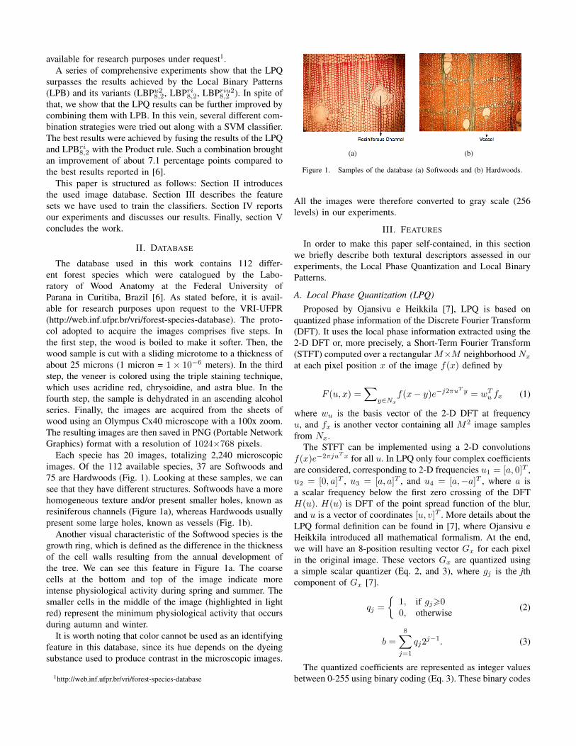
In order to get a better insight of these results we analyzesome classes that have an elevated error rate (between 40%and 65%). Figure 4 shows some samples of these classes.

Figures 4a and 4b show samples of Picea abies. For thisclass of forest species, both LPQ and LBP were able tocorrectly classify only 50% of the images. In such a case theLPQ performs slightly better since it can deal better with blur(e.g., Figure 4a) than LBP.

Another difficult class is the Mimosa bimucronata wherethe error rate ranges from 40 to 50%. As we can observefrom Figures 4c and 4d the same species has quite a differentdefinition of cells and intensity. A similar problem occurs withsamples of the class Eucalyptus grandis, depicted in Figures4e and 4f.

B. Invariance to Rotation

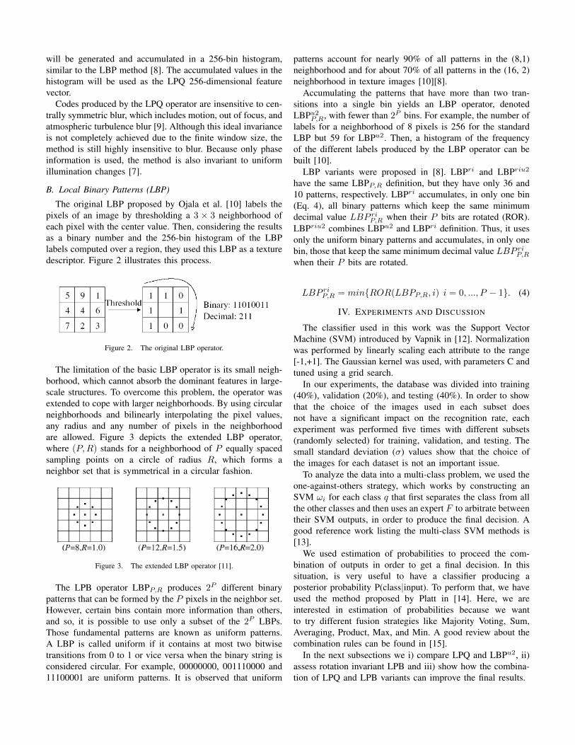
Analyzing the misclassified images, we have just observeddifferences on their orientations (Fig. 5). These differences areconsequence of the slides’ displacement on the microscopeduring image acquisition process. It is important to mentionthat we did not apply any filter to correct the rotation to theimages in our experiments.

Two configurations of rotation invariant LBP were tried out,both of them with eight neighbors and different distances. Asreported in Table II, the best results for LBPri and LBPriu2

were achieved for the distance two. LBPri8,2 achieved betterresults than LBPriu28,2 , but both of them were worse than thoseachieved by traditional LBPu28,2.

We observed that LBPriu28,2 and LBPri8,2 have correctlyclassified most of those images with differences on theirorientation, like the ones shown in Figure 5. However, theoverall recognition rate decreased. By analyzing the database,we observed a small number of images with some kind ofrotation. Besides LBPu2, LBPri, and LBPriu2 have featurevectors of 59, 36, and 10 components, respectively. So, this

(a) (b)

(c) (d)

(e) (f)

Figure 4. Species with recognition rates lower than 60%: (a-b) Picea abies,(c-d) Mimosa bimucronata, and (e-f) Eucalyptus grandis.

(a) (b)

Figure 5. Different angles.

impact in the recognition rates could be caused by a loss ofrepresentation capability as the number of elements in the LBPfeature vector decreases.

C. LPQ and LBP Classifiers Combination

In this last experiment we have combined LPQ and LBPvariants using two different strategies. In the first one we

Table IIRECOGNITION RATES FOR LBPri

8,2 AND LBPriu28,2 .

Features Feature % σVector Size

LBPri8,2 36 75.00 0.63

LBPriu28,2 10 54.68 1.77

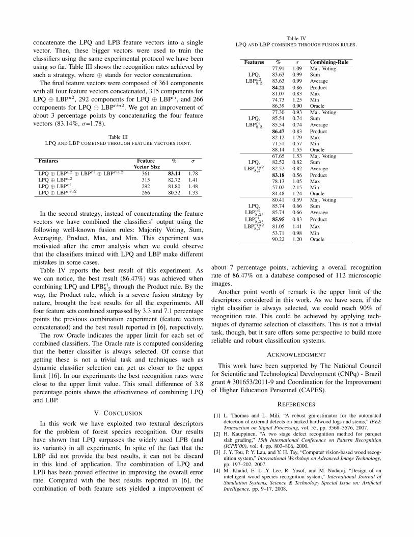
concatenate the LPQ and LPB feature vectors into a singlevector. Then, these bigger vectors were used to train theclassifiers using the same experimental protocol we have beenusing so far. Table III shows the recognition rates achieved bysuch a strategy, where ⊕ stands for vector concatenation.

The final feature vectors were composed of 361 componentswith all four feature vectors concatenated, 315 components forLPQ ⊕ LBPu2, 292 components for LPQ ⊕ LBPri, and 266components for LPQ ⊕ LBPriu2. We got an improvement ofabout 3 percentage points by concatenating the four featurevectors (83.14%, σ=1.78).

Table IIILPQ AND LBP COMBINED THROUGH FEATURE VECTORS JOINT.

Features Feature % σVector Size

LPQ ⊕ LBPu2 ⊕ LBPri ⊕ LBPriu2 361 83.14 1.78LPQ ⊕ LBPu2 315 82.72 1.41LPQ ⊕ LBPri 292 81.80 1.48LPQ ⊕ LBPriu2 266 80.32 1.33

In the second strategy, instead of concatenating the featurevectors we have combined the classifiers’ output using thefollowing well-known fusion rules: Majority Voting, Sum,Averaging, Product, Max, and Min. This experiment wasmotivated after the error analysis when we could observethat the classifiers trained with LPQ and LBP make differentmistakes in some cases.

Table IV reports the best result of this experiment. Aswe can notice, the best result (86.47%) was achieved whencombining LPQ and LPBri8,2 through the Product rule. By theway, the Product rule, which is a severe fusion strategy bynature, brought the best results for all the experiments. Allfour feature sets combined surpassed by 3.3 and 7.1 percentagepoints the previous combination experiment (feature vectorsconcatenated) and the best result reported in [6], respectively.

The row Oracle indicates the upper limit for each set ofcombined classifiers. The Oracle rate is computed consideringthat the better classifier is always selected. Of course thatgetting these is not a trivial task and techniques such asdynamic classifier selection can get us closer to the upperlimit [16]. In our experiments the best recognition rates wereclose to the upper limit value. This small difference of 3.8percentage points shows the effectiveness of combining LPQand LBP.

V. CONCLUSION

In this work we have exploited two textural descriptorsfor the problem of forest species recognition. Our resultshave shown that LPQ surpasses the widely used LPB (andits variants) in all experiments. In spite of the fact that theLBP did not provide the best results, it can not be discardin this kind of application. The combination of LPQ andLPB has been proved effective in improving the overall errorrate. Compared with the best results reported in [6], thecombination of both feature sets yielded a improvement of

Table IVLPQ AND LBP COMBINED THROUGH FUSION RULES.

Features % σ Combining-Rule77.91 1.09 Maj. Voting

LPQ, 83.63 0.99 SumLBPu2

8,2 83.63 0.99 Average84.21 0.86 Product81.07 0.83 Max74.73 1.25 Min86.39 0.90 Oracle77.30 0.93 Maj. Voting

LPQ, 85.54 0.74 SumLBPri

8,2 85.54 0.74 Average86.47 0.83 Product82.12 1.79 Max71.51 0.57 Min88.14 1.55 Oracle67.65 1.53 Maj. Voting

LPQ, 82.52 0.82 SumLBPriu2

8,2 82.52 0.82 Average83.18 0.56 Product78.13 1.05 Max57.02 2.15 Min84.48 1.24 Oracle80.41 0.59 Maj. Voting

LPQ, 85.74 0.66 SumLBPu2

8,2, 85.74 0.66 AverageLBPri

8,2, 85.95 0.83 ProductLBPriu2

8,2 81.05 1.41 Max53.71 0.98 Min90.22 1.20 Oracle

about 7 percentage points, achieving a overall recognitionrate of 86.47% on a database composed of 112 microscopicimages.

Another point worth of remark is the upper limit of thedescriptors considered in this work. As we have seen, if theright classifier is always selected, we could reach 90% ofrecognition rate. This could be achieved by applying tech-niques of dynamic selection of classifiers. This is not a trivialtask, though, but it sure offers some perspective to build morereliable and robust classification systems.

ACKNOWLEDGMENT

This work have been supported by The National Councilfor Scientific and Technological Development (CNPq) - Brazilgrant # 301653/2011-9 and Coordination for the Improvementof Higher Education Personnel (CAPES).

REFERENCES

[1] L. Thomas and L. Mili, “A robust gm-estimator for the automateddetection of external defects on barked hardwood logs and stems,” IEEETransaction on Signal Processing, vol. 55, pp. 3568–3576, 2007.

[2] H. Kauppinen, “A two stage defect recognition method for parquetslab grading,” 15th International Conference on Pattern Recognition(ICPR’00), vol. 4, pp. 803–806, 2000.

[3] J. Y. Tou, P. Y. Lau, and Y. H. Tay, “Computer vision-based wood recog-nition system,” International Workshop on Advanced Image Technology,pp. 197–202, 2007.

[4] M. Khalid, E. L. Y. Lee, R. Yusof, and M. Nadaraj, “Design of anintelligent wood species recognition system,” International Journal ofSimulation Systems, Science & Technology Special Issue on: ArtificialIntelligence, pp. 9–17, 2008.

[5] P. L. Paula Filho, L. S. Oliveira, A. S. Britto Jr., and R. Sabourin, “For-est species recognition using color-based features,” 20th InternationalConference on Pattern Recognition (ICPR2010), pp. 4178–4181, 2010.

[6] J. G. Martins, L. S. Oliveira, S. Nisgoski, and R. Sabourin, “A databasefor automatic classification of forest species,” Machine Vision andApplications, 2012.

[7] V. Ojansivu and J. Heikkila, “Blur insensitive texture classificationusing local phase quantization,” in Proceedings of the 3rd internationalconference on Image and Signal Processing, ser. ICISP ’08, 2008, pp.236–243.

[8] T. Ojala, M. Pietikainen, and T. Maenpaa, “Multiresolution gray-scaleand rotation invariant texture classification with local binary patterns,”Pattern Analysis and Machine Intelligence, IEEE Transactions on,vol. 24, no. 7, pp. 971 –987, jul 2002.

[9] M. R. Banham and A. K. Katsaggelos, “Digital image restoration,”Signal Processing Magazine, IEEE, vol. 14, no. 2, pp. 24–41, mar 1997.

[10] T. Ojala, M. Pietikinen, and D. Harwood, “A comparative study oftexture measures with classification based on featured distributions,” Pat-tern Recognition, vol. 29, no. 1, pp. 51 – 59, 1996. [Online]. Available:http://www.sciencedirect.com/science/article/pii/0031320395000674

[11] C. Shan, S. Gong, and P. W. McOwan, “Facial expression recognitionbased on local binary patterns: A comprehensive study,” Image andVision Computing, vol. 27, no. 6, pp. 803 – 816, 2009.

[12] V. Vapnik, Statistical Learning Theory. John Wiley and Sons, 1998.[13] C.-W. Hsu and C.-J. Lin, “A comparison of methods for multi-class

support vector machines,” IEEE Transactions on Neural Networks,vol. 13, pp. 415–425, 2002.

[14] J. Platt, “Probabilistic outputs for support vector machines and compar-isons to regularized likelihood methods,” in Advances in Large MarginClassifiers, A. S. et al, Ed. MIT Press, 1999, pp. 61–74.

[15] J. Kittler, M. Hatef, R. P. W. Duin, and J. Matas, “On combiningclassifiers,” IEEE Trans. Pattern Anal. Mach. Intell., vol. 20, 1998.

[16] A. Ko, R. Sabourin, A. Britto, and L. S. Oliveira, “Pairwise fusion matrixfor combining classifiers,” Pattern Recognition, no. 40, pp. 2198–2210,2007.