Combining Geometric and Appearance Priorsfor Robust Homography Estimation

Eduard Serradell1, Mustafa Ozuysal2, Vincent Lepetit2,Pascal Fua2, and Francesc Moreno-Noguer1

1Institut de Robotica i Informatica Industrial, CSIC-UPC, Barcelona, Spain2 Computer Vision Laboratory, EPFL, Lausanne, Switzerland

eserradell@iri.upc.edu, mustafa.oezuysal@epfl.ch,

vincent.lepetit@epfl.ch, pascal.fua@epfl.ch, fmoreno@iri.upc.edu

Abstract. The homography between pairs of images are typically com-puted from the correspondence of keypoints, which are established byusing image descriptors. When these descriptors are not reliable, eitherbecause of repetitive patterns or large amounts of clutter, additionalpriors need to be considered. The Blind PnP algorithm makes use ofgeometric priors to guide the search for matches while computing cam-era pose. Inspired by this, we propose a novel approach for homographyestimation that combines geometric priors with appearance priors of am-biguous descriptors. More specifically, for each point we retain its bestcandidates according to appearance. We then prune the set of poten-tial matches by iteratively shrinking the regions of the image that areconsistent with the geometric prior. We can then successfully computehomographies between pairs of images containing highly repetitive pat-terns and even under oblique viewing conditions.

Key words: homography estimation, robust estimation, RANSAC

1 Introduction

Computing homographies from point correspondences has received much atten-tion because it has many applications, such as stitching multiple images intopanoramas [1] or detecting planar objects for Augmented Reality purposes [2,3]. All existing methods assume that the correspondences are given a priori andusually rely on an estimation scheme that is robust both to noise and to outrightmismatches. As a result, the best ones tolerate significant error rates among thecorrespondences but break down when the rate becomes too large. Therefore,in cases when the correspondences cannot be established reliably enough such

This work has been partially funded by the Spanish Ministry of Science and Inno-vation under CICYT projects PAU DPI2008-06022 and UbROB DPI2007-61452; byMIPRCV Consolider Ingenio 2010 CSD2007-00018; by the EU project GARNICSFP7-247947 and by the Swiss National Science Foundation.

2 E.Serradell et al.

(a) (b)

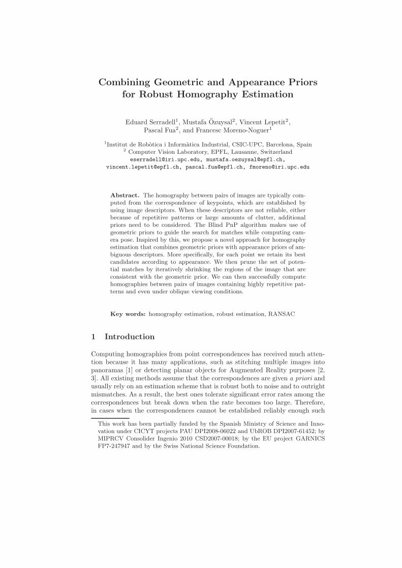
Fig. 1. Detecting an oblique planar pattern. (a) PROSAC fails due to high number ofoutliers caused by the extreme camera angle. (b) Our approach can reassign correspon-dences as the homography space is explored and can recover the correct homography.

as in the presence of repetitive patterns, they can easily fail. In this paper, weintroduce an estimation scheme that performs well even under such demandingcircumstances.

We build upon the so-called Blind PnP approach [4] that was designed tosimultaneously establish 2D to 3D correspondences and estimate camera pose.To this end, it exploits the fact that, in general, some prior on the camera poseis often available. This prior is modeled as a Gaussian Mixture Model that isprogressively refined by hypothesizing new correspondences. Incorporating eachnew one in a Kalman filter rapidly reduces the number of potential 2D matchesfor each 3D point and makes it possible to search the pose space sufficiently fastfor the method to be practical.

Unfortunately, when going from exploring the 6-dimensional camera-posespace to the 8-dimensional space of homographies, the size of the search spaceincreases to a point where a naive extension of the Blind PnP approach failsto converge. This is in part because this approach is suboptimal in the sensethat it does not exploit image-appearance, which can be informative even inambiguous cases. In general, any given 2D point can be associated to severalpotentially matching 2D points with progressively decreasing levels of confidence.To exploit this fact without having to depend on a prori correspondences, weexplicitly use similarity of image appearance to remove both low confidencepotential correspondences and pose prior modes that do not result in promisingmatch candidates. We further improve convergence rates by ignoring potentialmatches that are least likely to reduce the covariances of the Kalman filter.

As a result, our algorithm performs well even in highly oblique views of planarscenes containing repetitive patterns such as the one of Fig. 1. In such scenes,

Combining Geom. and App. Priors for Robust Homography Estimation 3

interest point detectors exhibit very poor repeatability and, as a result, even sucha reliable algorithm as PROSAC [5] fails because a priori correspondences aretoo undependable. We will use benchmark data to quantify the effectiveness ofour approach. We will also show that it can be used to improve the convergenceproperties of the original Blind PnP.

2 Related Work

Correspondence-based approaches to computing homographies between imagestend to rely on a RANSAC-style strategy [7] to reject mismatches that pointmatchers inevitably produce in complex situations. In practice, this means se-lecting and validating small sets of correspondences until an acceptable solutionis found. The original RANSAC algorithm remains a valid solution, as long asthe proportion of mismatches remains low enough. Early approaches [8, 9] toincreasing the acceptable mismatch rate, introduced a number of heuristic crite-ria to stop the search, which were only satisfied in very specific and unrealisticsituations. Other methods, before selecting candidate matches, consider all pos-sible ones and organize them in data structures that can be efficiently accessed.Indexing methods, such as Hash tables [10, 11] and Kd-trees [12], or clusters inthe pose space [13, 14] have been used for this purpose. Nevertheless, even withinfast access data structures, these methods become computationally intractablewhen there are too many points.

Several more sophisticated versions of the RANSAC algorithm, such as GuidedSampling [15], PROSAC [5], and ARRSAC [16] have been proposed and theyaddress the problem by using image-appearance to speed up the search for con-sistent matches. However, when the images contain repetitive structure resultingin unreliable keypoints and truly poor matches such as in Fig. 1, even they canfail. In those conditions, simple outlier rejection techniques [25] also fail.

In the context of the so-called PnP problem, which involves recovering cam-era pose from 3D to 2D correspondences, the Softposit algorithm [17] addressesthis problem by iteratively solving for pose and correspondences, achieving anefficient solution for sets of about 100 feature points. Yet, this solution is proneto failure when different viewpoints may yield similar projections of the 3Dpoints. This is addressed in the Blind PnP [4] by introducing weak pose priors,that constrain where the camera can look at, and guide the search for corre-spondences. Although achieving good results, both these solutions are limitedto about a hundred feature points, and are therefore impractical in presence ofthe number of feature points that a standard keypoint detector would find in ahigh resolution textured image.

In this paper, we show that the response of local image descriptors, evenwhen they are ambiguous and unreliable, may still be used in conjunction withgeometric priors to simultaneously solve for homographies and correspondences.This lets us tackle very complex situations with many feature points and repet-itive patterns, where current state-of-the-art algorithms fail.

4 E.Serradell et al.

3 Algorithm Overview

We next give a short overview of the algorithm we propose to simultaneouslyrecover the homography that relates two images of a planar scene and pointcorrespondences between them. We achieve this by

– Introducing a Geometric prior: We first define the search space for thehomography. It can cover the whole homography space or depending on theapplication can be constrained to cover a smaller space, for example to limitthe range of rotations or scales. We generate random homography samples inthis search space, as we detail in Section 4. We then fit a Gaussian MixtureModel (GMM) to these samples using the Expectation Maximization (EM)algorithm. The modes of this GMM forms the geometric prior.

– Introducing an Appearance prior: For each keypoint pair (xi,xj), wedefine the appearance prior as the similarity score sA(xi,xj) given by a localmatching algorithm.

– Iteratively solving for correspondences and homography: We explorethe modes of the geometric prior until enough consistent matches and thecorresponding homography are found. Section 5 gives the details, we providea brief overview here. This prior exploration starts at each prior mode meanwith the covariance matrices estimated by EM. Each model point is trans-fered using the homography, while the projection of its covariance defines asearch region for potential matches. We use the appearance prior to limitnumber of correspondences as explained in Section 4.3. The homographyestimate and its covariance are iteratively updated by a Kalman filter thatuses the best correspondences as measurements until the covariance becomesnegligible.

4 Priors on the Search Space

In this section we give details on how both geometric and appearance priors arebuilt, and on the pruning strategies we define to robustly reduce the numberof keypoints and eliminate unnecessary geometric priors. As we will show inSection 6, this lets us to handle highly textured images with a large number ofinterest points.

4.1 Parameterization of Homographies

To define a search space for the homography, we first need to select a parame-terization for the homography. Then we can randomly sample these parametersto obtain homography samples from the search space. A natural choice is todecompose the homography as

x′ = A′ (R− tvTπ

)A−1x ,

where A and A′ are the intrinsic parameters of the cameras, R and t theirextrinsic transformation, vπ is the unit normal to the scene plane, x′ is a point

Combining Geom. and App. Priors for Robust Homography Estimation 5

on the target image, and x is a point on the model image. However this is anover-parameterization and has even more than 8 parameters. Therefore we lookfor a direct parameterization of the 8 DOF of a homography:

x′ = Hx ,

Once such possibility is to consider its action on a unit square centeredaround the origin. We can therefore parameterize the homography with thecoordinates of the resulting quadrangle as H(u1, v1, u2, v2, u3, v3, u4, v4). Giventhe 2D correspondences between the four vertices of the quadrangle, we can findthe corresponding homography as the solution of the linear system

MH = 0 , (1)

whereM is a 8×9 matrix made of the vertices coordinates, HT = [H11, . . . ,H33]T,

Hij are the components of the matrix H, and 0 is a vector of zeros. We can alsowork out its Jacobian evaluated at (u1, v1, u2, v2, u3, v3, u4, v4)

JH =

⎡⎢⎣

δH11

δu1

δH12

δu1. . . δH33

δu1

......

...δH11

δu4

δH12

δu4. . . δH33

δu4

⎤⎥⎦ ,

which we will need when computing the projection of covariances defining thesearch space for correspondences. Therefore, we can propagate a covariance as-signed to the prior modes to the model image as follows

Σw = JuvJHΣusJTHJT

uv

and Juv stands for the Jacobian of the homography evaluated for the imagepoint (u′, v′). It can be written as

Juv = δu′/δh =1

z′

[xT 0 −u′xT

0 xT −v′xT

], (2)

where u′ = (u′, v′)T = (x′/z′, y′/z′)T are the inhomogeneous coordinates.

4.2 Geometric Prior

To define the geometric prior, we use a set of homography samples representingthe set of all possible deformations of the image plane. If an estimate of theinternal parameters is available, it can be parametrized directly by the camerarotation and translation. We apply all deformations obtained in this way tothe unit square and obtain a set of sample parameter values corresponding tocoordinates of the deformed square. Using EM we fit a GMM to these samples,which yields G Gaussian components with 8-vectors {h1, . . . ,hg} for the means,and 8 × 8 covariance matrices {Σh

1 , . . . ,Σhg}. Note that it is possible to use a

larger or smaller set of deformations to define the geometric prior depending onthe constraints imposed by the application.

6 E.Serradell et al.

−2 −1 0 1 2−1.5

−1

−0.5

0

0.5

1

1.5

2

x

y

Keypoint Selection

Detected Feature PointsEstimated projectionsAppearance candidatesSelected candidates

20 40 60 80 1000

10

20

30

40

Inf

Prior order

RM

S E

rror

(pi

x)

Prior Re−ordering

EM based ranking

Appearance based ranking

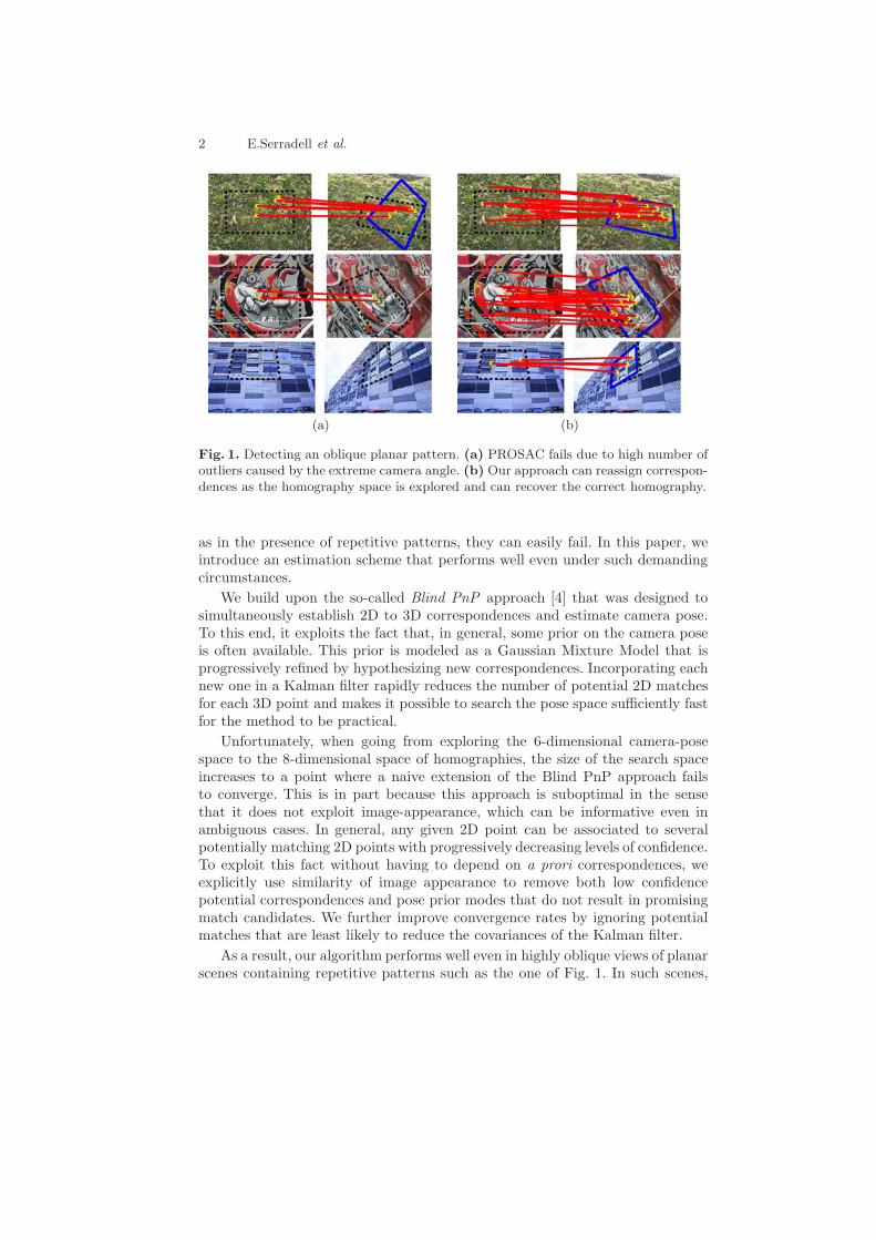
Fig. 2. Pruning based on appearance. Left: For the projected model point on theimage, a direct adaptation of the Blind PnP would select every point within the uncer-tainty ellipse as a correspondence candidate. Considering appearance, our algorithmonly selects a small subset of them. Right: We plot the residual re-projection error foreach prior mode. Modes with lower indexes have higher rank and are explored first. Aresidual error of ‘Inf’ denotes a mode that does not converge to a good homography. Ablind approach explores the modes following the EM ranking therefore spending timeon ones that eventually do not result in good pose hypotheses. We use appearance torank the modes and explore a smaller subset without missing out the good ones.

4.3 Appearance Prior

To compute the similarity score between keypoint pairs, we have chosen to workwith the Ferns keypoint classifier [18] since it is fast and directly outputs aprobability distribution for each keypoint. However, our approach can use otherstate-of-the-art keypoint descriptors such as SIFT [19] or SURF [20], providedthat we can assign a similarity score to each hypothetical correspondence. Weexploit the computed score in two ways.

Pruning keypoints. Using appearance, we are able to reduce for each modelpoint, the whole set of potential candidates to a small selection of keypoints.The probability of finding a good match remains unaltered but the computa-tional cost of the algorithm is highly reduced. Fig. 2 shows the effect of pruningkeypoints. Note that it significantly reduces the number of potential matches.Additionally, we select only the most promising model keypoints that have ahigh scoring correspondence given by Ferns posterior distributions.

Pruning prior modes. To avoid exploring all modes of the geometric prior,we assign an appearance score to each one and eliminate the ones with lowerscores. To compute the appearance score SA for each mode hg, we transformthe set of model keypoints xi only once using the corresponding homographygiven by the mode, pick the ones that has only one potential candidate, andsum their similarity scores as

SA(hg) =1

M

M∑i=1

δ(xi ∈ C1) · sA(xi,xj), (3)

Combining Geom. and App. Priors for Robust Homography Estimation 7

where sA(xi,xj) is the similarity score of xi and its corresponding target key-point xj , C1 is the set of model keypoints with exactly one match candidate, andδ(.) is the indicator function that returns 1 if its argument is true or 0 otherwise.Fig. 2 depicts an example with G = 100 pose prior modes.

5 Estimating Correspondences and Homography

At detection time, we are given a set of M 2D points {xi} on the model imageand a set of N keypoints {xj} on the target image. Some of the model keypointscorrespond to detected features and some do not. Similarly, the homography maytransfer some of the model points to locations without any nearby keypoints.Our goal is to find both the correct homography H and as many point-to-pointcorrespondences as possible. LetM be a set of (xi,xj) pairs that represents theserecovered correspondences and Nnd be the subset of points for which no matchcan be established. We want to find the correct homography H and matches Mby minimizing

Error(H) =∑

(xi,xj)∈M||xj −Hxi||2 + γ|Nnd| , (4)

where γ is a penalty term that penalizes unmatched points.

Pose Space Exploration. We sequentially explore the pose prior modes bypicking candidate correspondences (xi,xj) and by updating the mode mean hg

and covariance Σg using the standard Kalman update equations,

h+g = hg +K (xj −Hgxi) ,

Σp+g = (I−KJ(xi))Σ

pg ,

where Hg is the homography corresponding to the mean vector hg, K is theKalman Gain, and I is the Identity matrix.

Candidate Selection. We use the covariance Σhg to restrict the number of

potential of matches between the points of the two images, by transferring themodel points xi using the homography to target image coordinates ui and theprojected covariances Σu

i . Error propagation yields

Σui = J(xi)Σ

hgJ(xi)

T , (5)

where J(xi) = JuvJH is the Jacobian of the transfer by homography Hgxi thatwe derived in Section 4. This defines a search region for the point xi, and weonly consider the detected image features u′

j such that

(ui − u′j)

TΣui (ui − u′

j) ≤ T 2 (6)

as potential matches for xi and only if they have a high enough similarity scoresA(ui,u

′j). T is a threshold chosen to achieve a specified degree of confidence,

based on the cumulative chi-squared distribution.

8 E.Serradell et al.

(a) (b)

(c) (d)

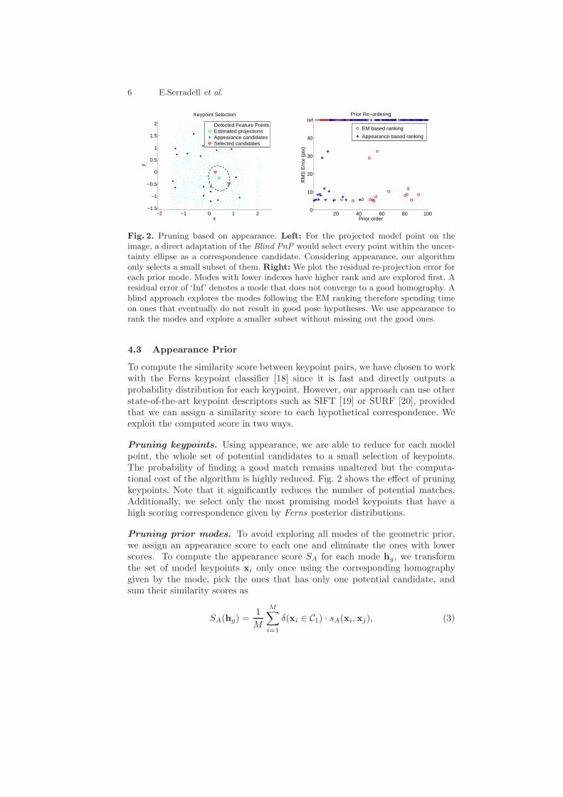
Fig. 3. Pose space exploration. (a) Exploration of a prior mode starts by pickingcorrespondences with small projected covariance hence high confidence. (b) In thethird iteration, covariances are much smaller. Also the selected candidate has largercovariance than the 3 model points indicated with yellow ellipses. Their locations willnot be updated and they will not be considered for future Kalman updates. (c) Thefourth point is picked despite its large uncertainty since the other points close to thecenter will not help to reduce covariance as much. (d) The covariances are very smallas four points have already been used to update the homography. We can still use afifth point to remove the uncertainty close to the borders.

Blind PnP selects the point with minimum number of potential candidatesinside the threshold ellipse. When the number of potential candidates is high(n ≈ 5) this works just fine because it minimizes the number of possible combi-nations. In our case, taking advantage of the appearance, n becomes very smalland most of the points have either zero or one potential candidate. In this case,this blind selection process becomes random and the updates may not convergeto a good homography.

Another way to select the point to introduce into the Kalman Filter is theone proposed by [21, 22] that selects at each iteration the most informative point,which would make the algorithm converge quickly to the optimal solution. How-ever, this method is sensitive to outliers and the optimal solution may be hardto find if it is found at all.

As none of the preceding methods was suitable, we implemented a new ap-proach for candidate selection. Instead of trying to converge as fast as possible,we choose the point which has the minimum number of correspondences, has

Combining Geom. and App. Priors for Robust Homography Estimation 9

1 2 3 40

2

4

6

8

10

Img ID

RM

S E

rro

r (p

ix)

Naive selection (BlindPnP) Naive selection + App. pruning Selection using MI + App. pruning

5 10 15 20 25 300

2

4

6

8

10

Pose prior

Tim

e (s

)

Naive selection (BlindPnP) Naive selection + App. pruning Selection using MI + App. pruning

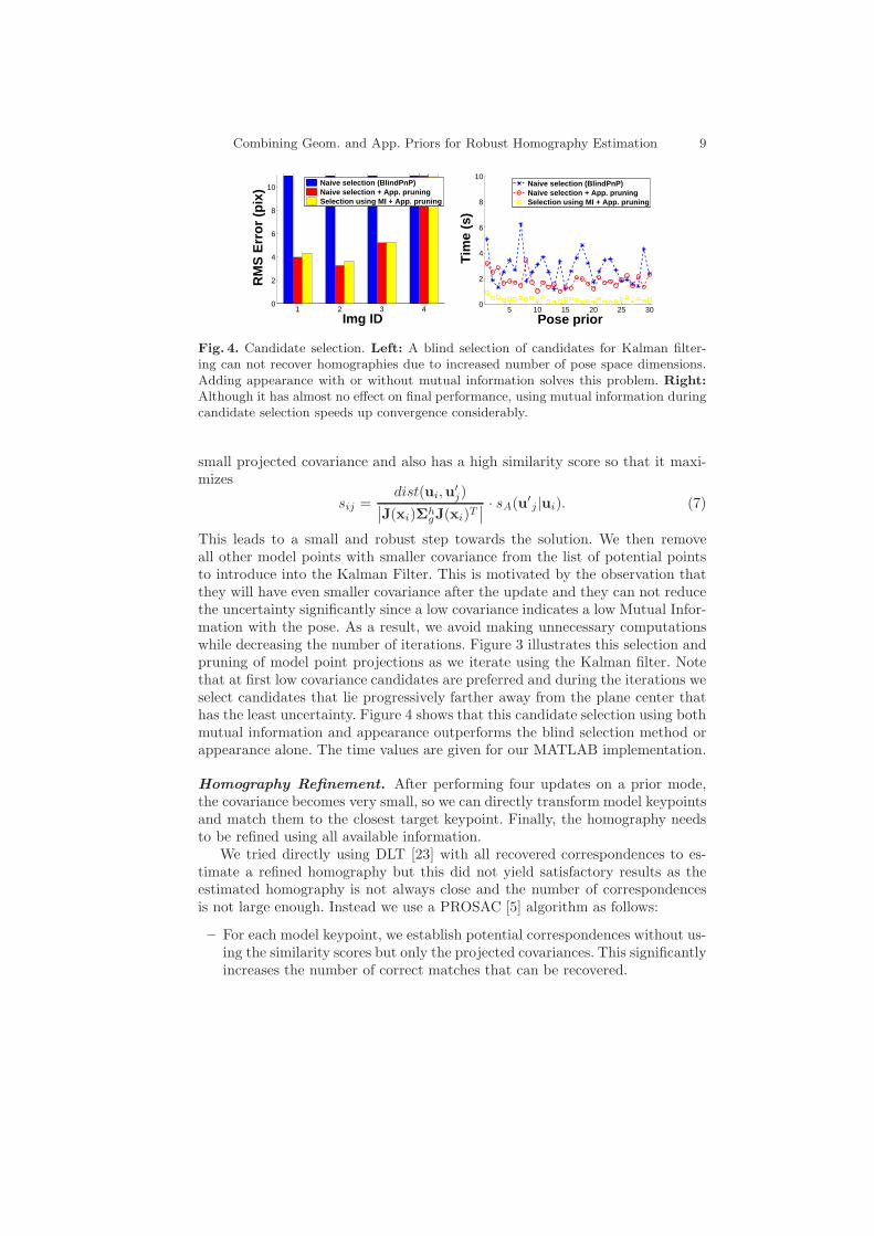
Fig. 4. Candidate selection. Left: A blind selection of candidates for Kalman filter-ing can not recover homographies due to increased number of pose space dimensions.Adding appearance with or without mutual information solves this problem. Right:Although it has almost no effect on final performance, using mutual information duringcandidate selection speeds up convergence considerably.

small projected covariance and also has a high similarity score so that it maxi-mizes

sij =dist(ui,u

′j)∣∣J(xi)Σh

gJ(xi)T∣∣ · sA(u′

j|ui). (7)

This leads to a small and robust step towards the solution. We then removeall other model points with smaller covariance from the list of potential pointsto introduce into the Kalman Filter. This is motivated by the observation thatthey will have even smaller covariance after the update and they can not reducethe uncertainty significantly since a low covariance indicates a low Mutual Infor-mation with the pose. As a result, we avoid making unnecessary computationswhile decreasing the number of iterations. Figure 3 illustrates this selection andpruning of model point projections as we iterate using the Kalman filter. Notethat at first low covariance candidates are preferred and during the iterations weselect candidates that lie progressively farther away from the plane center thathas the least uncertainty. Figure 4 shows that this candidate selection using bothmutual information and appearance outperforms the blind selection method orappearance alone. The time values are given for our MATLAB implementation.

Homography Refinement. After performing four updates on a prior mode,the covariance becomes very small, so we can directly transform model keypointsand match them to the closest target keypoint. Finally, the homography needsto be refined using all available information.

We tried directly using DLT [23] with all recovered correspondences to es-timate a refined homography but this did not yield satisfactory results as theestimated homography is not always close and the number of correspondencesis not large enough. Instead we use a PROSAC [5] algorithm as follows:

– For each model keypoint, we establish potential correspondences without us-ing the similarity scores but only the projected covariances. This significantlyincreases the number of correct matches that can be recovered.

10 E.Serradell et al.

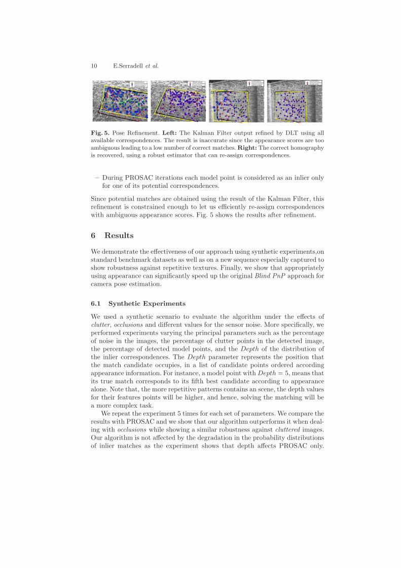
Fig. 5. Pose Refinement. Left: The Kalman Filter output refined by DLT using allavailable correspondences. The result is inaccurate since the appearance scores are tooambiguous leading to a low number of correct matches.Right: The correct homographyis recovered, using a robust estimator that can re-assign correspondences.

– During PROSAC iterations each model point is considered as an inlier onlyfor one of its potential correspondences.

Since potential matches are obtained using the result of the Kalman Filter, thisrefinement is constrained enough to let us efficiently re-assign correspondenceswith ambiguous appearance scores. Fig. 5 shows the results after refinement.

6 Results

We demonstrate the effectiveness of our approach using synthetic experiments,onstandard benchmark datasets as well as on a new sequence especially captured toshow robustness against repetitive textures. Finally, we show that appropriatelyusing appearance can significantly speed up the original Blind PnP approach forcamera pose estimation.

6.1 Synthetic Experiments

We used a synthetic scenario to evaluate the algorithm under the effects ofclutter, occlusions and different values for the sensor noise. More specifically, weperformed experiments varying the principal parameters such as the percentageof noise in the images, the percentage of clutter points in the detected image,the percentage of detected model points, and the Depth of the distribution ofthe inlier correspondences. The Depth parameter represents the position thatthe match candidate occupies, in a list of candidate points ordered accordingappearance information. For instance, a model point withDepth = 5, means thatits true match corresponds to its fifth best candidate according to appearancealone. Note that, the more repetitive patterns contains an scene, the depth valuesfor their features points will be higher, and hence, solving the matching will bea more complex task.

We repeat the experiment 5 times for each set of parameters. We compare theresults with PROSAC and we show that our algorithm outperforms it when deal-ing with occlusions while showing a similar robustness against cluttered images.Our algorithm is not affected by the degradation in the probability distributionsof inlier matches as the experiment shows that depth affects PROSAC only.

Combining Geom. and App. Priors for Robust Homography Estimation 11

0.80.60.40.200

20

40

60

80

100

Occlusions(%)

Det

ecti

on

(%)

Our method PROSAC

(a) (b) (c) (d)

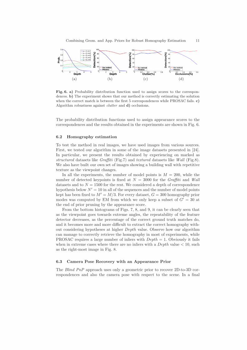
Fig. 6. a) Probability distribution function used to assign scores to the correspon-dences. b) The experiment shows that our method is correctly estimating the solutionwhen the correct match is between the first 5 correspondences while PROSAC fails. c)Algorithm robustness against clutter and d) occlusions.

The probability distribution functions used to assign appearance scores to thecorrespondences and the results obtained in the experiments are shown in Fig. 6.

6.2 Homography estimation

To test the method in real images, we have used images from various sources.First, we tested our algorithm in some of the image datasets presented in [24].In particular, we present the results obtained by experiencing on marked asstructured datasets like Graffiti (Fig.7) and textured datasets like Wall (Fig.8).We also have built our own set of images showing a building wall with repetitivetexture as the viewpoint changes.

In all the experiments, the number of model points is M = 200, while thenumber of detected keypoints is fixed at N = 3000 for the Graffiti and Walldatasets and to N = 1500 for the rest. We considered a depth of correspondencehypothesis below N ′ = 10 in all of the sequences and the number of model pointskept has been fixed to M ′ = M/3. For every dataset, G = 300 homography priormodes was computed by EM from which we only keep a subset of G′ = 30 atthe end of prior pruning by the appearance score.

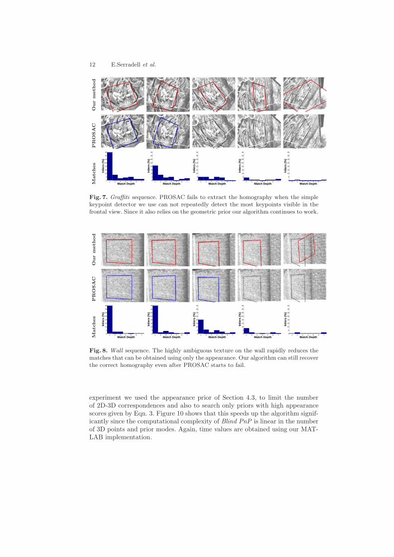
From the bottom histograms of Figs. 7, 8, and 9, it can be clearly seen thatas the viewpoint goes towards extreme angles, the repeatability of the featuredetector decreases, as the percentage of the correct ground truth matches do,and it becomes more and more difficult to extract the correct homography with-out considering hypotheses at higher Depth value. Observe how our algorithmcan manage to correctly retrieve the homography in most of experiments, whilePROSAC requires a large number of inliers with Depth = 1. Obviously it failswhen in extreme cases where there are no inliers with a Depth value < 10, suchas the right-most image in Fig. 8.

6.3 Camera Pose Recovery with an Appearance Prior

The Blind PnP approach uses only a geometric prior to recover 2D-to-3D cor-respondences and also the camera pose with respect to the scene. In a final

12 E.Serradell et al.

Ourm

eth

od

PROSAC

Matc

hes

1 2 3 4 5 6 70

5

10

15

20

25

30

35

40

Match Depth

Inlie

rs (

%)

1 2 3 4 5 6 70

5

10

15

20

25

30

35

40

Match Depth

Inlie

rs (

%)

1 2 3 4 5 6 70

5

10

15

20

25

30

35

40

Match Depth

Inlie

rs (

%)

1 2 3 4 5 6 70

5

10

15

20

25

30

35

40

Match Depth

Inlie

rs (

%)

1 2 3 4 5 6 70

5

10

15

20

25

30

35

40

Match Depth

Inlie

rs (

%)

Fig. 7. Graffiti sequence. PROSAC fails to extract the homography when the simplekeypoint detector we use can not repeatedly detect the most keypoints visible in thefrontal view. Since it also relies on the geometric prior our algorithm continues to work.

Ourm

eth

od

PROSAC

Matc

hes

1 2 3 4 5 6 70

5

10

15

20

25

30

35

40

Match Depth

Inlie

rs (

%)

1 2 3 4 5 6 70

5

10

15

20

25

30

35

40

Match Depth

Inlie

rs (

%)

1 2 3 4 5 6 70

5

10

15

20

25

30

35

40

Match Depth

Inlie

rs (

%)

1 2 3 4 5 6 70

5

10

15

20

25

30

35

40

Match Depth

Inlie

rs (

%)

1 2 3 4 5 6 70

5

10

15

20

25

30

35

40

Match Depth

Inlie

rs (

%)

Fig. 8. Wall sequence. The highly ambiguous texture on the wall rapidly reduces thematches that can be obtained using only the appearance. Our algorithm can still recoverthe correct homography even after PROSAC starts to fail.

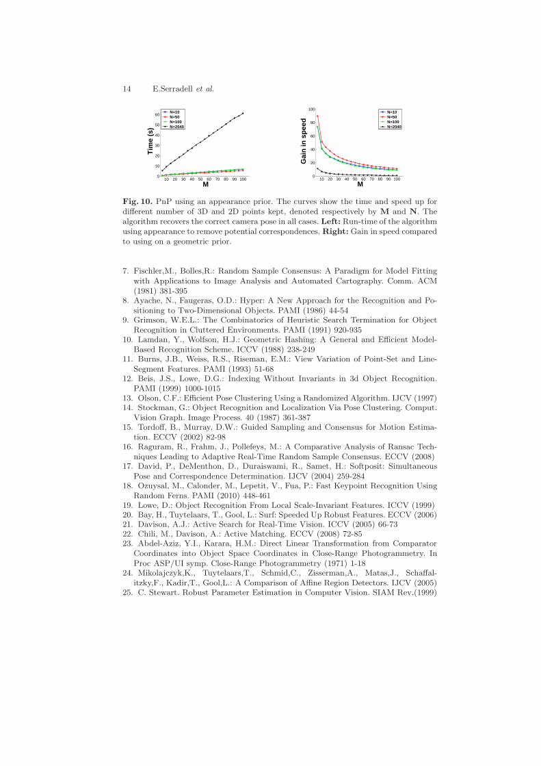
experiment we used the appearance prior of Section 4.3, to limit the numberof 2D-3D correspondences and also to search only priors with high appearancescores given by Eqn. 3. Figure 10 shows that this speeds up the algorithm signif-icantly since the computational complexity of Blind PnP is linear in the numberof 3D points and prior modes. Again, time values are obtained using our MAT-LAB implementation.

Combining Geom. and App. Priors for Robust Homography Estimation 13

Ourm

eth

od

PROSAC

Matc

hes

1 2 3 4 5 6 70

5

10

15

20

25

30

35

40

Match Depth

Inlie

rs (

%)

1 2 3 4 5 6 70

5

10

15

20

25

30

35

40

Match Depth

Inlie

rs (

%)

1 2 3 4 5 6 70

5

10

15

20

25

30

35

40

Match Depth

Inlie

rs (

%)

1 2 3 4 5 6 70

5

10

15

20

25

30

35

40

Match Depth

Inlie

rs (

%)

1 2 3 4 5 6 70

5

10

15

20

25

30

35

40

Match Depth

Inlie

rs (

%)

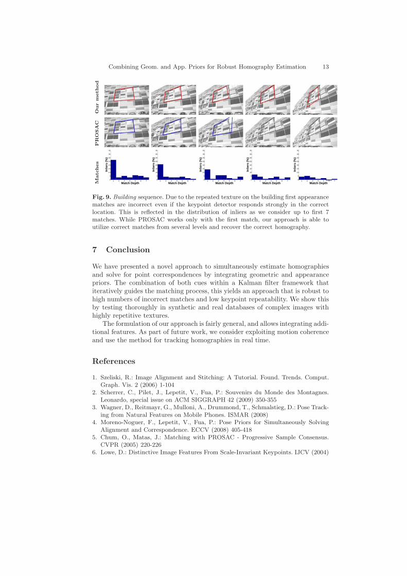
Fig. 9. Building sequence. Due to the repeated texture on the building first appearancematches are incorrect even if the keypoint detector responds strongly in the correctlocation. This is reflected in the distribution of inliers as we consider up to first 7matches. While PROSAC works only with the first match, our approach is able toutilize correct matches from several levels and recover the correct homography.

7 Conclusion

We have presented a novel approach to simultaneously estimate homographiesand solve for point correspondences by integrating geometric and appearancepriors. The combination of both cues within a Kalman filter framework thatiteratively guides the matching process, this yields an approach that is robust tohigh numbers of incorrect matches and low keypoint repeatability. We show thisby testing thoroughly in synthetic and real databases of complex images withhighly repetitive textures.

The formulation of our approach is fairly general, and allows integrating addi-tional features. As part of future work, we consider exploiting motion coherenceand use the method for tracking homographies in real time.

References

1. Szeliski, R.: Image Alignment and Stitching: A Tutorial. Found. Trends. Comput.Graph. Vis. 2 (2006) 1-104

2. Scherrer, C., Pilet, J., Lepetit, V., Fua, P.: Souvenirs du Monde des Montagnes.Leonardo, special issue on ACM SIGGRAPH 42 (2009) 350-355

3. Wagner, D., Reitmayr, G., Mulloni, A., Drummond, T., Schmalstieg, D.: Pose Track-ing from Natural Features on Mobile Phones. ISMAR (2008)

4. Moreno-Noguer, F., Lepetit, V., Fua, P.: Pose Priors for Simultaneously SolvingAlignment and Correspondence. ECCV (2008) 405-418

5. Chum, O., Matas, J.: Matching with PROSAC - Progressive Sample Consensus.CVPR (2005) 220-226

6. Lowe, D.: Distinctive Image Features From Scale-Invariant Keypoints. IJCV (2004)

14 E.Serradell et al.

10 20 30 40 50 60 70 80 90 1000

10

20

30

40

50

60

M

Tim

e (s

)

N=10 N=50 N=100 N=2040

10 20 30 40 50 60 70 80 90 1000

20

40

60

80

100

M

Gai

n in

sp

eed

N=10 N=50 N=100 N=2040

Fig. 10. PnP using an appearance prior. The curves show the time and speed up fordifferent number of 3D and 2D points kept, denoted respectively by M and N. Thealgorithm recovers the correct camera pose in all cases. Left: Run-time of the algorithmusing appearance to remove potential correspondences. Right: Gain in speed comparedto using on a geometric prior.

7. Fischler,M., Bolles,R.: Random Sample Consensus: A Paradigm for Model Fittingwith Applications to Image Analysis and Automated Cartography. Comm. ACM(1981) 381-395

8. Ayache, N., Faugeras, O.D.: Hyper: A New Approach for the Recognition and Po-sitioning to Two-Dimensional Objects. PAMI (1986) 44-54

9. Grimson, W.E.L.: The Combinatorics of Heuristic Search Termination for ObjectRecognition in Cluttered Environments. PAMI (1991) 920-935

10. Lamdan, Y., Wolfson, H.J.: Geometric Hashing: A General and Efficient Model-Based Recognition Scheme. ICCV (1988) 238-249

11. Burns, J.B., Weiss, R.S., Riseman, E.M.: View Variation of Point-Set and Line-Segment Features. PAMI (1993) 51-68

12. Beis, J.S., Lowe, D.G.: Indexing Without Invariants in 3d Object Recognition.PAMI (1999) 1000-1015

13. Olson, C.F.: Efficient Pose Clustering Using a Randomized Algorithm. IJCV (1997)14. Stockman, G.: Object Recognition and Localization Via Pose Clustering. Comput.

Vision Graph. Image Process. 40 (1987) 361-38715. Tordoff, B., Murray, D.W.: Guided Sampling and Consensus for Motion Estima-

tion. ECCV (2002) 82-9816. Raguram, R., Frahm, J., Pollefeys, M.: A Comparative Analysis of Ransac Tech-

niques Leading to Adaptive Real-Time Random Sample Consensus. ECCV (2008)17. David, P., DeMenthon, D., Duraiswami, R., Samet, H.: Softposit: Simultaneous

Pose and Correspondence Determination. IJCV (2004) 259-28418. Ozuysal, M., Calonder, M., Lepetit, V., Fua, P.: Fast Keypoint Recognition Using

Random Ferns. PAMI (2010) 448-46119. Lowe, D.: Object Recognition From Local Scale-Invariant Features. ICCV (1999)20. Bay, H., Tuytelaars, T., Gool, L.: Surf: Speeded Up Robust Features. ECCV (2006)21. Davison, A.J.: Active Search for Real-Time Vision. ICCV (2005) 66-7322. Chili, M., Davison, A.: Active Matching. ECCV (2008) 72-8523. Abdel-Aziz, Y.I., Karara, H.M.: Direct Linear Transformation from Comparator

Coordinates into Object Space Coordinates in Close-Range Photogrammetry. InProc ASP/UI symp. Close-Range Photogrammetry (1971) 1-18

24. Mikolajczyk,K., Tuytelaars,T., Schmid,C., Zisserman,A., Matas,J., Schaffal-itzky,F., Kadir,T., Gool,L.: A Comparison of Affine Region Detectors. IJCV (2005)

25. C. Stewart. Robust Parameter Estimation in Computer Vision. SIAM Rev.(1999)