Combining Extended Retiming and Unfolding for Rate …toneil/research/papers/journals/jvsp05.pdf ·...

Journal of VLSI Signal Processing 39, 273–293, 2005c© 2005 Springer Science + Business Media, Inc. Manufactured in The Netherlands.

Combining Extended Retiming and Unfolding for Rate-OptimalGraph Transformation

TIMOTHY W. O’NEILDepartment of Comp. Science, University of Akron, Akron, OH 44325-4003

EDWIN H.-M. SHADepartment of Comp. Science, Erik Jonsson School of Eng. & C.S., Box 830688, MS EC 31,

University of Texas at Dallas, Richardson, TX 75083-0688

Received December 1, 2003; Revised December 1, 2003; Accepted May 7, 2004

Abstract. Many computation-intensive iterative or recursive applications commonly found in digital signal pro-cessing and image processing applications can be represented by data-flow graphs (DFGs). The execution of alltasks of a DFG is called an iteration, with the average computation time of an iteration the iteration period. A greatdeal of research has been done attempting to optimize such applications by applying various graph transformationtechniques to the DFG in order to minimize this iteration period. Two of the most popular are retiming and unfold-ing, which can be performed in tandem to achieve an optimal iteration period. However, the result is a transformedgraph which is much larger than the original DFG. To the authors’ knowledge, there is no technique which can becombined with minimal unfolding to transform a DFG into one whose iteration period matches that of the optimalschedule under a pipelined design. This paper proposes a new technique, extended retiming, which does just this.We construct the appropriate retiming functions and design an efficient retiming algorithm which may be applieddirectly to a DFG instead of the larger unfolded graph. Finally, we show through experiments the effectiveness ofour algorithms.

Keywords: scheduling, data-flow graphs, retiming, unfolding, graph transformation, timing optimization

1. Introduction

For real-time or computation-intensive applicationssuch as DSP, image processing and simulations for fluiddynamics, it is important to optimize the execution rateof a design. Because the most time-critical parts of suchapplications are loops, we must explore the parallelismembedded in the repetitive pattern of a loop. A loopcan be modeled as a data-flow graph (DFG) [1, 2].The nodes of a DFG represent tasks, while edges be-tween nodes represent data dependencies among tasks.Each edge may contain a number of delays (i.e. regis-ters) indicating loop-carried dependencies. This modelis widely used in many fields, including circuitry [3],

digital signal processing [4] and program descriptions[5, 6].

To meet the desired throughput, it becomes neces-sary to use multiple processors or multiple functionalunits. In our previous work [7–10], we proposed an ef-ficient algorithm, extended retiming, which transformsa DFG into an equivalent graph with maximum par-allelization and minimum schedule length wheneverthe DFG meets certain very narrow criteria. Therefore,there remain applications for which our original frame-work will not deliver the best possible result. We wishto correct this exclusion in this paper.

The execution of all tasks of a DFG is called aniteration. A very popular strategy for maximizing

274 O’Neil and Sha

parallelism is to transform the original graph byscheduling multiple iterations simultaneously, a tech-nique known as unfolding [11]. While the graph be-comes much larger, the average computation time ofan iteration (the iteration period) can be reduced. Inour previous work, we demonstrated that extended re-timing allows us to achieve an optimal iteration periodwhen the iteration period is an integer. In this paper,we refine our original scheme so that extended retim-ing may be combined with unfolding. We then showthat this combination achieves optimality for all cases.In fact, we will see that this combination attains an opti-mal result while doing a minimal amount of unfolding.We find that the combination of traditional retimingand unfolding does not correctly characterize the im-plementation using a pipelined design and, therefore,tends to give a large unfolding factor. Thus we not onlymaximize parallelism by using extended retiming, butwe also minimize the size of the necessary transformedgraph.

In addition to unfolding, one of the more effectivegraph transformation techniques is retiming, where de-lays are redistributed among the edges so that the func-tion of the DFG G remains the same, but the lengthof the longest zero-delay path (the clock period ofG, denoted cl(G)) is decreased. This technique wasintroduced in [3] to optimize the throughput of syn-chronous circuits, and has since been used extensivelyin such diverse areas as software pipelining [12, 13] andhardware-software codesign [14, 15]. We have shownpreviously that this traditional form of retiming [7] can-not produce optimal results when applied individually.The same is true for unfolding (as we will see), but thecombination of traditional retiming and unfolding willachieve optimality [1].

To illustrate these ideas, consider the example ofFig. 1(a). The numbers inside the nodes represent com-putation times. The short bar-lines cutting the edgefrom node C to node B (hereafter referred to by theordered pair (C, B)) represent inter-iteration dependen-cies between these nodes. In other words, the two linescutting (C, B) tell us that task B of our current itera-tion depends on data produced by task C two iterationsago. This representation of such a dependency is calleda delay on the edge of the DFG.

It is clear that the clock period of this graph is 14,obtained from the path from A to C . Since an iterationof the DFG may be scheduled within 14 time units as inFig. 1(b), the iteration period of this graph is also 14.However, if we were to remove a delay from (C, A)

Figure 1. (a) A data-flow graph; (b) The schedule for the DAG partof Fig. 1(a).

and place it on (A, B), the iteration period (i.e. clockperiod) would be reduced to 10 while not affecting thefunction of the graph. (This assumes the existence ofmultiple processors within the system. Indeed, we willnot consider resource-constrained scheduling in thispaper.) The example shows how retiming may be usedto adjust the iteration period of a DFG.

How small can we make our iteration period? Sinceretiming preserves the number of delays in a cycle, theratio of a cycle’s total computation time to its delaycount remains fixed regardless of retiming. The maxi-mum of all such ratios, called the iteration bound [16],acts as a lower bound on the iteration period. In thecase of Fig. 1(a), there are only two cycles, the smallone between nodes B and C with time-to-delay ratio42 = 2, and the large one involving all nodes with ratio144 . Thus the iteration bound for the graph is 7

2 .Since the computation times of all nodes are integral,

it seems impossible to get a fractional iteration period.However, recall that the iteration period is the aver-age time to complete an iteration. If we can completetwo iterations of our graph in 7 time units, the averagewill equal our lower bound, and our graph will be rate-optimal. To get these iterations together in our graph,we must unfold the graph. If we can unfold our graphf times to achieve this lower bound, our schedule issaid to be rate-optimal, and f is called a rate-optimalunfolding factor. We are interested in finding the min-imum such unfolding factor.

As an example, let us unfold the graph of Fig. 1(a) bya factor of 2, as shown in Fig. 2(a). (We will discuss ouralgorithm for doing this in detail later.) We can schedulean iteration of this new graph—which is equivalent toscheduling two iterations of our original graph—in thesame 14 time units. We have doubled the size of our

Combining Extended Retiming and Unfolding 275

Figure 2. (a) The DFG of Fig. 1(a) unfolded by a factor of 2; (b)Figure 2(a) retimed by extended retiming to be rate-optimal; (c) Theoptimal schedule for the retimed graph.

graph, but we have also reduced our iteration period to7. We can now retime this unfolded graph as we didabove to reduce our clock period to 10, which furtherreduces the iteration period to 5. Unfortunately thisis the best we can do by unfolding twice and usingtraditional retiming.

If we were permitted to move a delay inside of A,as shown in Fig. 2(b), our clock period would become7, the iteration period would become 7

2 and we wouldhave optimized our graph, as we can see by the schedulein Fig. 2(c). This is the advantage of extended retim-ing over traditional retiming: we are allowed to movedelays not only from edge to edge, but from edge tovertex. We see from this that the combination of tradi-tional retiming and unfolding does not completely give

Figure 3. (a) The DFG of Fig. 1(a) unfolded by a factor of 4; (b)Figure 3(a) retimed by traditional retiming to be rate-optimal.

the correct representation of the graph’s schedule, es-pecially when we assume a pipelined implementation.

We should note that, when we talk about movingdelays inside of nodes, we do not mean that we arephysically placing registers inside of functional units ina circuit. We are merely describing an abstraction for agraph which provides for a feasible schedule with looppipelining, as this example shows. Traditional retimingis not powerful enough to capture such a schedule, andso may produce an inferior result.

An unfolding of 2 combined with extended retimingoptimizes the graph of Fig. 1(a). If we limit ourselves totraditional retiming, we must unfold the original DFGfour times, as shown in Fig. 3(a). After we retime as inFig. 3(b) in addition to unfolding, we can now sched-ule 4 iterations of the original graph in 14 time steps,reducing our iteration period without retiming to 7

2 . Wesee that traditional retiming tends to overestimate therate-optimal unfolding factor, resulting in a graph thatrequires more resources for execution.

Note that the graph optimized by extended retimingand unfolding is half the size of that optimized by tra-ditional retiming and unfolding. There is a very clearadvantage in using extended retiming, but there are cur-rently two drawbacks to this method:

1. As proposed, extended retiming only permits theplacement of a single delay inside any node. This istoo severe a limitation for what we want to do now.


For instance, note that if we had been allowed toremove two delays from (C, A) in Fig. 1(a) and usethem to split node A into three pieces of sizes 4, 4and 2, we would have achieved an almost optimaliteration period of 4 even before unfolding.

2. The only method for applying extended retimingand unfolding is the one we’ve outlined: unfold thegraph and then retime. Since retiming is much moreexpensive than unfolding in terms of computationtime, it is preferable to first apply extended retimingto the smaller original graph, then unfolding. How-ever, we must be certain that the two operationscan be performed in any order and still achieveoptimality.

We also have the question of knowing exactly howmuch to unfold a graph before it can be optimized. Aswe’ve said, unfolding dramatically increases the sizeof the graph we’re working with, so we don’t want todo any more unfolding than is absolutely necessary.

We accomplish the following in this paper:

1. We will demonstrate a new form of retiming, ex-tended retiming, which achieves an optimal resultwhile requiring the use of a smaller unfolded graph,and thus fewer resources.

2. Our original definition of extended retiming wasconstructed with the assumption that at most onedelay may be placed within a given node. We nowmodify this definition to accommodate the possi-bility that multiple delays are placed inside a node.This permits us to combine extended retiming withunfolding.

3. When we wish to apply unfolding and extended re-timing to a graph, we have two options: first retimethe graph then unfold it, or unfold it then retime theunfolded graph. We will show that these two meth-ods are equivalent and construct the correspondingretiming functions.

4. Because of this equivalence, we are able to designan efficient extended retiming algorithm which canbe applied directly to the original graph. In fact, wewill show that we can construct an extended retim-ing for a graph G in O(|V ‖E |) time where V andE are the vertex and edge sets for G, respectively.This improves our previous work, the applicationof which could produce a retiming function onlyfor the larger unfolded graph.

5. Finally, we will demonstrate that the minimum rate-optimal unfolding factor for a data-flow graph is thedenominator of the irreducible form of the graph’s

iteration bound. Thus we have devised a techniquethat, when combined with unfolding by the min-imum rate-optimal unfolding factor, transforms agraph into one whose iteration period matches thatof the rate-optimal schedule. To the best of ourknowledge, this is the first method that can do this.

The rest of the paper is organized as follows. In thenext section, we will formalize fundamental conceptssuch as data-flow graphs, unfolding and clock period.The theme of this paper is presented next, along withsome introductory results. Sections 4 and 5 containthe paper’s most significant result, the proof of the in-terchangeability of extended retiming and unfolding.We then design our efficient algorithm and show itseffectiveness when applied to graphs whose iterationsbounds are one or larger, which encompasses all non-trivial examples. The minimal rate-optimal unfoldingfactor for a DFG is determined next, followed by de-tailed examples of this work. Finally, we summarizeour work and provide questions for further study.

2. Background

In this section, we wish to present the definitions andresults relating to unfolding and unfolded graphs. Wewill rely on this previously-presented background ma-terial [17, 11] heavily as we establish our new results.

2.1. Unfolding and Unfolded Graphs

Formally, a data-flow graph (DFG) is a finite, directed,weighted graph G = 〈V, E, d, t〉 where V is a set ofcomputation nodes, E is a set of edges between nodes,d : E → N is a function representing the delay count ofeach edge, and t : V → N representing the computationtime of each node. A path in G is a connected sequenceof nodes and edges. We will use the notations D(p) andT (p) to represent the total computation time and totaldelay count of path p, respectively.

Now, let f be a positive integer. We wish to alter ourgraph so that f consecutive iterations (i.e. executionsof all of a DFG’s tasks) are visible simultaneously. Todo this, we create f copies of each node, replacing nodeu in the original graph by the nodes u1 through u f inour new graph. This process is known as unfoldingthe graph G f times and results in the unfolded graphG f = 〈V f , E f , d f , t f 〉. The unfolding transformationwas introduced in [11] and has been widely discussed


Figure 4. (a) A sample DFG; (b) This DFG unfolded by a factorof 3.

in the literature. As a brief example, if we unfold thegraph in Fig. 4(a) by a factor of 3, the result is Fig. 4(b).

As we can see from this example, the vertex set V f

is simply the union of the f copies of each node in V .Since they are all exact copies, the computation timesremain the same, i.e. t f (u f ) = t(u) for every copy u f

of u ∈ V . Each edge of G also corresponds to f copiesin the unfolded graph. However, the delay counts of thecopies do not match that of the original edge. In fact,an edge (ui , v j ) having d delays in the unfolded graphrepresents a precedence relation between node u in thei th iteration and node v in iteration d · f + j in theoriginal graph. This idea is formalized in the followingtheorem, which is proven in [1].

Theorem 2.1. Let e = (u, v) be an edge in DFG G.Let f be an unfolding factor for G. Then:1. For all i, j ∈ {0, 1, 2, . . . , f − 1}, there exists an

edge e f = (ui , v j ) in G f if and only if d(e) = d f (e f )·f + j − i .

2. For all integers i, j ∈ {0, 1, 2, . . . , f −1} with j ≡(i +d(e)) mod f , there exists an edge e f = (ui , v j )in G f with d f (e f ) = � d(e)

f � if i ≤ j and d(e)f �

otherwise.3. The f copies of edge e in G f are the edges ei =

(ui , v(i+d(e)) mod f ) for i = 0, 1, 2, . . . , f − 1.4. The total number of delays of the f copies of edge

e is d(e), i.e. d(e) = ∑ f −1i=0 d f (ei ).

Despite implications in the literature to the con-trary [11], it is possible to construct a DFG whichcannot be unfolded to become rate-optimal. For ex-ample, consider the unit-time DFG of Fig. 5(a)with iteration bound 2. When unfolded by a fac-tor of f > 1, it becomes the graph of Fig. 5(b).We see that there is a zero-delay path consisting ofthe nodes A f −1, B f −1, C f −1, B f −2, C f −2, . . . , B0, C0

with computation time 2 · f + 1. Hence the iterationperiod of the unfolded graph will always be greaterthan or equal to 2 + 1

f , which is always strictly largerthan the iteration bound. This shows that retiming isnecessary for achieving an optimal result.

Finally, a classic result from [3] characterized theupper bound of a graph’s cycle period in terms ofthe computation time of its longest zero-delay path.The analogous result for an unfolded graph is provenin [1].

Figure 5. (a) A unit-time DFG; (b) This DFG unfolded by a factorof f .


Theorem 2.2. Let G be a DFG, c a potential cycleperiod and f an unfolding factor.1. cl(G f ) = max{T (p) : p ∈ G is a path with D(p) <

f }.2. cl(G f ) ≤ c if and only if, for every path p in G with

T (p) > c, D(p) ≥ f .

2.2. Static Scheduling

Given a DFG G, a clock period c and an unfoldingfactor f , we construct the scheduling graph Gs =〈V, E, w, t〉 by reweighting each edge e = (u, v) ac-cording to the formula w(e) = d(e) − f

c · t(u). We thenfurther alter Gs by adding a node v0 and zero-weightdirected edges from v0 to every other node in G. Fig-ure 6(b) shows the scheduling graph of the example inFig. 6(a) when c = 3 and f = 1. It can be shown that,if c

f is a feasible iteration period, then the schedul-ing graph contains no negative-weight cycles. Definesh(v) for every node v to be the length of the shortestpath from v0 to v in this modified Gs . For example,in the graph of Fig. 6(b), we note that sh(A) = 0 and

Figure 6. (a) A DFG; (b) The scheduling graph with c = 3 andf = 1; (c) The schedule with cycle period 3.

sh(B) = sh(C) = − 13 . It takes O(|V ||E |) time to com-

pute sh(v) for every node v [18].The definitions for iteration, iteration period, iter-

ation bound and rate-optimal have been given previ-ously. Note that Fig. 6(c) demonstrates one rate-optimalschedule for the DFG in Fig. 6(a). The relationship be-tween the iteration bound of a DFG and the DFG’sscheduling graph is given in Lemma 3.1 of [18]:

Lemma 2.3. Let G be a DFG, c a clock period andf an unfolding factor. B(G) ≤ c

f if and only if thescheduling graph Gs contains no cycles having neg-ative weight.

We formally define an integral schedule on a DFG Gto be a function s : V × N → Z where the starting timeof node v in the i th iteration (i ≥ 0) is given by s(v, i). Itis a legal schedule if s(u, i)+t(u) ≤ s(v, i+d(e)) for alledges e = (u, v) and iterations i . For example, the legalintegral schedule of Fig. 6(c) is S3(v, i) = 3(i − sh(v))for all nodes v and iterations i , where the values forsh(v) are derived from the graph of Fig. 6(b).

A legal schedule is a repeating schedule for cycle pe-riod c and unfolding factor f if s(v, i + f ) = s(v, i)+cfor all nodes v and iterations i . It’s easy to see thatS3(v, i) is an example of a repeating schedule. A re-peating schedule can be represented by its first itera-tion, since a new occurrence of this partial schedule canbe started at the beginning of every interval of c clockticks to form the complete legal schedule. If an oper-ation of the partial schedule is assigned to the sameprocessor in each occurrence of the partial schedule,we say that our schedule is static.

Since the iteration bound for the graph of Fig. 6(a) is3, and all nodes of this graph are 3 or smaller, Theorems2.3 and 3.5 of [18] tell us that the minimum achiev-able cycle period for this graph is 3. We can producethe static DFG schedule in Fig. 6(c) by constructingthe scheduling graph and computing sh(v) for each ofthe nodes. We can then use this information to createthe schedule of Fig. 6(c) by applying the formula fromthe above discussion to create the schedule; for this ex-ample S3(A, 0) = 0 and S3(B, 0) = S3(C, 0) = 3 ·13 = 1.

3. Extended Retiming

In a previous paper [7], we demonstrated that tradi-tional retiming and unfolding did not necessarily resultin an optimal schedule when applied individually, and


devised a form of retiming which was equivalent toDFG scheduling. This definition and work dependedon the assumption that unfolding did not take place, soany node of a graph could be split at most once.

We demonstrated in the Introduction that, while thecombination of traditional retiming and unfolding al-ways yields an optimal result, the combination of ex-tended retiming and unfolding yields the same result inmany cases while requiring the use of a much smallergraph. We now devise a new, more general form of ourextended retiming that will work even when used inconjunction with unfolding. The definition used in [7]then becomes a special case of these results.

An extended (or f-extended) retiming of a DFGG = 〈V, E, d, t〉 is a function r : V → Z × Q f where,for all v ∈ V , r (v) = i + ( r1

t(v) ,r2

t(v) , . . . ,r f

t(v) ) forsome integers i, r1, r2, . . . , r f where 0 ≤ rk < t(v) fork = 1, 2, . . . , f . We view the integer constant i as thenumber of delays that are pushed to each outgoingedge of v, while the f -tuple lists the positions ofdelays within the node v. Note that a value of zerowithin the f -tuple is merely a placeholder used to sim-plify our notation; we can’t have a delay at this posi-tion. Also for simplicity we will express the f -tupleas 1

t(v) (r1, r2, . . . , r f ) or as a single fraction r1t(v) when

f = 1.We can see from this definition that r (v) can be

viewed as consisting of an integer part and a fractionalpart. We will use the notation ır (v) to denote the valueof this integer part, while r (v) will be the numberof non-zero coordinates in the f -tuple. We will alsoassume throughout this paper that the elements of anf -tuple are listed in increasing order.

For example, consider the graph of Fig. 7(a). A3-extended retiming with r (A) = 1 + 1

9 (0, 2, 5),r (B) = 1 and r (C) = 0 results in the retimed graphof Fig. 7(b). For this retiming, ır (A) = ır (B) = 1 andır (C) = 0, while r (A) = 2 and r (B) = r (C) = 0.Simple as-early-as-possible (AEAP) scheduling ap-plied to Fig. 7(b) yields Fig. 7(c).

As with standard retiming, we will denote the DFGretimed by r as Gr = 〈V, E, dr , t〉. When we definethe delay count of the edge e = (u, v) after retiming,we must remember to include delays within each end-node as well as delays along the edge itself. We alsowant the new definition to be analogous to our tradi-tional one: the old delay count of the edge (d(e)), plusthe number of delays drawn from each incoming edge(ır (u) + r (u)), minus the number of delays pushed toeach outgoing edge (ır (v)).

Figure 7. (a) Another sample DFG; (b) This DFG retimed; (c) TheAEAP schedule for Fig. 7(b).

Previously, we defined a path p to be a con-nected sequence of nodes and edges, with D(p) be-ing the path’s total delay count. If we now requireD(p) to count the delays both among the nodes andalong the edges of p, we can easily obtain theseproperties:

Lemma 3.1. Let G be a DFG without split nodes andr an extended retiming.1. The retimed delay count on the edge e = (u, v) is

dr (u → v) = d(e) + ır (u) − ır (v) + r (u).2. The retimed delay count on the path p : u ⇒ v is

Dr (u ⇒ v) = D(p) + ır (u) − ır (v) + r (u).3. The retimed delay count on the cycle � ∈ G is

Dr (�) = D(�).

Given an edge e = (u, v), we use dr (u → v) to de-note the total number of delays along an edge, includ-ing delays contained within the end nodes u and v.However, we will refer to the number of delays on theedge not including delays within end nodes as dr (e)as in the traditional case. Using the example fromFig. 7(b), let e1 = (A, B), e2 = (B, C) and e3 = (C, A).Then dr (A → B) and dr (C → A) are each 2 due toa split end-node, even though dr (e1) and dr (e3) areeach zero, while dr (B → C) = dr (e2) = 1 since thereis no split end-node for this edge. As with traditional


retiming, an extended retiming is legal if dr (e) ≥ 0 forall edges e ∈ E and normalized if minv ır (v) = 0. Notetwo things:

1. If r is an extended retiming, then dr (u → v) =dr (e) + r (u) + r (v) for all edges e = (u, v) ∈ E .Therefore, if r is legal, dr (u → v) ≥ 0 for all edgese = (u, v) ∈ E since r (u) and r (v) are bothpositive by definition.

2. Any extended retiming can be normalized by sub-tracting minv ır (v) from all values ır (v).

We have defined a path above to be a connected se-quence of nodes and edges. This definition assumesthat a path includes all pieces of its initial and finalnodes. On the other hand, we will define a connectedsequence of nodes and edges which includes only someof the pieces of its initial and final nodes to be a sub-path. For example, consider the graph of Fig. 7(b). Anypath which begins or ends with node A must includeall three pieces of node A, while a subpath may beginor end at any of A’s pieces and does not have to containall of A. Thus a path is a subpath, but a subpath is notnecessarily a path.

It should be clear that some pieces of the end-nodesof a path are missing when we discuss a subpath. If anode u is split by r (u) delays, we can see that we areleft with r (u)+1 pieces which we can denote in orderas u0, u1,. . . , u r (u). So if we have a subpath from u j tovk , the delay count of the subpath will equal that of thepath from u to v, minus the j delays which separatethe first j + 1 pieces of u from one another, minusthe r (v) − k delays separating vk , vk+1,. . . , v r (v). Inshort,

Dr (u j ⇒ vk) = D(p) + ır (u) − ır (v) + r (u)

− r (v) + k − j,

where p is the path from u to v. Note that this is con-sistent with our previous lemma, since the path fromu to v is the same as the subpath from u0 to v r (v). Fi-nally, note that, in a graph G with split nodes, cl(G) isthe maximum computation time among all zero-delaysubpaths of G.

4. Unfolding Followed by Extended Retiming

In this section and the next, we will prove one of ourmajor results: that the combination of extended retim-

ing and unfolding yields the same minimal iterationperiod, no matter which transformation is performedfirst. We will do this in two steps. First, we wish toshow that, for every extended retiming of the unfoldedgraph which gives us a certain cycle period, we canconstruct a retiming on the original graph which yieldsthe same cycle period.

4.1. The Main Idea

To illustrate our idea, consider the graph of Fig. 7(a)with iteration bound 11

3 . In order to achieve an opti-mal iteration period, we must unfold this graph threetimes, as we will show later. Since we are merely seek-ing to construct a simple example which demonstratesour method, we will only unfold twice, producing thegraph in Fig. 8(a). The minimum cycle period that wecan achieve under these circumstances is 8, since 8 isthe smallest natural number which, when divided by2 (the unfolding factor), exceeds the iteration bound.

Figure 8. (a) The DFG of Fig. 7(a) unfolded twice; (b) This DFG’sschedule with cycle period 8; (c) This DFG retimed.


Thus, we use the method of [1] to schedule this graphwithin 8 time units, as shown in Fig. 8(b). Note thatwe’ve unfolded this graph as much as we want for thisexercise and will do no further unfolding. Thus, we canapply the result from [8], cutting the graph immediatelybefore the first occurrence of the last node to enter theschedule (shown here with a dashed line) and readingthe extended retiming immediately. This method givesus an extended retiming of

r (A0) = 15

9, r (A1) = 1

2

9,

r (B0) = r (B1) = r (C0) = 1, r (C1) = 0,

whose application to the graph in Fig. 8(a) results in thegraph in Fig. 8(c). If G is the graph in Fig. 7(a), then thegraph in Fig. 8(c) which has first been unfolded thenretimed is denoted as (G f )r .

We now wish to use this retiming on the unfoldedgraph to derive a retiming for the original graph. Whatwe will do is to add them using a special addition oper-ator ⊕ on the set of extended retimings for a particularnode which adds the integer parts of the retimings whileconcatenating the fractional parts. Formally, for eachnode u and positive integers i and j ,

r (ui ) ⊕ r (u j ) =(

ır (ui ) + 1

t(ui )(α1, . . . , αn)

)

⊕(

ır (u j ) + 1

t(u j )(β1, . . . , βm)

)

= (ır (ui ) + ır (u j ))

+ 1

t(u)(α1, . . . , αn, β1, . . . , βm).

(1)

Thus, for our example,

r (A) = 15

9⊕ 1

2

9= 2 + 1

9(5, 2), r (B) = 1 ⊕

1 = 2, r (C) = 1 ⊕ 0 = 1.

Normalizing this and reordering the 2-tuple into as-cending order gives us a 2-extended retiming of r (A) =1+ 1

9 (2, 5), r (B) = 1 and r (C) = 0, a retiming similarto the one that we found earlier to achieve the graph inFig. 9(a). (This graph, the version of G from Fig. 7(a)which is first retimed then unfolded, is denoted asGr, f .)

Note that there are some retimings resulting fromthis method that need special attention. As an example,

Figure 9. (a) The DFG of Fig. 7(a) retimed to have iteration period8/2; (b) A new data-flow graph; (c) The DFG of Fig. 9(b) retimed tohave iteration period 3/2.

we earlier unfolded the graph in Fig. 9(b) by a factorof two and retimed it via the function

r (Ai ) = 1, r (Bi ) = 1

2, r (Ci ) = 0

for i = 0, 1, to produce an optimized graph. Addingthese results in a retiming with r (A) = 2, r (B) =14 (2, 2) and r (C) = 0. This may look odd, since wehave the two delays inside node B next to each other(see Fig. 9(c)). Nonetheless, this is a legal extendedretiming which results in an optimal retimed graph.

4.2. The Result

Now that we’ve established what we want to do, let’sformalize our idea. In the next theorem, we demonstratethat, if it is possible for us to first unfold our graph andthen retime it to achieve a desired cycle period, then we


may also achieve that cycle period by first retiming thegraph and then unfolding. Because retiming takes moretime than unfolding, it is desirable to retime the smallergraph first, rather than unfolding and then retiming amuch larger graph.

Theorem 4.1. Let G be a data-flow graph withoutsplit nodes, c a cycle period and f an unfolding factor.For every legal extended retiming r f on the unfoldedgraph G f such that cl((G f )r f ) ≤ c, there exists a legalextended retiming r on the original graph G such thatcl(Gr, f ) ≤ c.

Proof: Using the operator defined in Eq. (1) above,define r : V → Z as

r (u) = r f (u0) ⊕ r f (u1) ⊕ · · · ⊕ r f (u f −1)

for each node u ∈ V . Note that this definition andEq. (1) imply that ır (u) = ∑ f −1

0 ır f (ui ) and r (u) =∑ f −10 r f (ui ). We must show that this is a legal retim-

ing and that cl(Gr, f ) ≤ c.

1. Let e : u → v be any edge in G; we want toshow that dr (e) ≥ 0. Now, by Theorem 2.1(3),there are f copies of this edge in the unfoldedgraph G f , the edges ei : ui → v(i+d(e)) mod f fori = 0, 1, 2, . . . , f − 1. Furthermore, since the ex-tended retiming r f is legal, d f (e f ) ≥ ır f (v f ) −ır f (u f ) + r f (v f ) for any edge e f from this set.Therefore,

ır (v) − ır (u) + r (v) =f −1∑i=0

(ır f

(v(i+d(e)) mod f

)

− ır f (ui ) + r f (vi ))

(2)

and so ır (v)− ır (u)+ r (v) ≤ ∑ f −10 d f (ei ) = d(e)

by Theorem 2.1(4). Thus

dr (e) = dr (u → v) − r (u) − r (v)

= d(e) + ır (u) − ır (v) − r (v) ≥ 0

and r is a legal extended retiming by definition.2. Let pi : ui ⇒ v j be any path in G f with T f (pi ) > c

for some integer i ∈ [0, f − 1]; then D f,r f (ui ⇒v j ) ≥ 1 by Theorem 2.2. Since

D f,r f (ui ⇒ v j ) = D f (pi ) + ır f (ui ) − ır f (v j )

+ r f (ui )

by Lemma 3.1, we may conclude that

ır f (v j ) − ır f (ui ) − r f (ui ) ≤ D f (pi ) − 1

for this integer i . Now, this path corresponds toa path p : u ⇒ v in the original graph G andj = (i + d(p)) mod f . Thus the work we’ve doneholds for any copy of this path in the unfolded graph.In other words, our inequality is true for any in-teger i ∈ [0, f − 1]. Thus, if we extend Eq. (2)and Theorem 2.1(4) from edges to paths, we seethat

ır (v) − ır (u) − r (u) ≤f −1∑i=0

(D f (pi ) − 1)

= D(p) − f,

and so Dr (u ⇒ v) = D(p) + ır (u) − ır (v) + r (u)≥ f whenever Tr (u ⇒ v) = T (p) > c. By Theo-rem 2.2, cl(Gr, f ) ≤ c.

5. Extended Retiming Followed by Unfolding

The first half of our desired result was fairly simple;this half will be much more complicated. We will startby establishing a couple of facts from [17] which ex-plore the relationship between traditional retiming andunfolding. We will then outline our method for expand-ing this result to deal with extended retiming, followedby a formal proof.

5.1. Traditional Retiming Followed by Unfolding

The statement and proof of our desired result (The-orem 5.1, below) for traditional retimings appears asLemma 3.3 in [1], so we will only briefly discuss themain idea of that proof. Given a data-flow graph G,nodes u and v and positive integers i and j smaller thanan unfolding factor f , we can show that there is a one-to-one correspondence between the edges e f = (ui , v j )in G f and er, f = (u(i−r (u)) mod f , v( j−r (v)) mod f ) in Gr, f .Let r f be a retiming on G f and let d f,r f (e f ) be the de-lay count of e f after we apply r f to G f . Now, givena retiming r on G, we want to find a function r f suchthat d f,r f (e f ) = dr, f (er, f ) for all edges e f in G f , wheredr, f (er, f ) is the delay count of the corresponding er, f

in Gr, f . Since d f,r f (e f ) = d f (e f ) + r f (ui ) − r f (v j ) by


the analogue of Lemma 3.1(1) for traditional retimings,our condition becomes

r f (ui ) − r f (v j ) = dr, f (er, f ) − d f (e f )

∀e f = (ui , v j ). (3)

Since (3) constitutes a consistent linear system withinteger solution r f , our theorem is proved.

5.2. The Main Idea

We now wish to prove the correctness of our assertionusing this idea applied to extended retimings. We haveseen that an extended retiming on a data-flow graphgives us instructions on how to split a node into smallerpieces. What we will do is to construct a new graph, re-placing each split node with the proper smaller pieces.This new graph can then be retimed to have optimalclock period by a traditional retiming which can bederived from the given extended one. Having trans-lated our original graph and extended retiming to anew graph and traditional retiming, we may then ap-ply our above theorem, derive a retiming for the un-folded graph, and then translate back to our originalgraph.

Consider the sample data-flow graph G in Fig. 10(a)below. Recall that the 2-extended retiming with r (A) =1 + 1

9 (2, 5), r (B) = 1 and r (C) = 0 applied to Gachieves an iteration period of 4. We now wish to usethis function to construct an extended retiming for Gunfolded twice.

We’ve seen that our extended retiming calls for usto split node A into three pieces with computationtimes 2, 3 and 4, respectively, while the other nodesremain whole. So, if we split A into three separatenodes with appropriate computation times, as shownin Fig. 10(b), the resulting graph can achieve rate op-timality via traditional retiming. We will call such agraph an extended graph, and designate the extendedgraph produced by a DFG G and extended retiming r asX G,r .

As we’ve pointed out, we should be able to retimeX G,r to be rate optimal using only a traditional retim-ing, i.e. a retiming without a fractional component. Re-call that the fractional part of r (A) above called for theplacement of delays between the first and second piecesand second and third pieces of A, with one delay pass-ing through the node and onto the outgoing edge; thusthree delays come into A while only one leaves. In ourextended graph, this is equivalent to passing three de-

Figure 10. (a) Our sample DFG; (b) The resulting extended graph;(c) This extended graph retimed to have iteration period 4.

lays through node A0, leaving one on the edge (A0, A1)and passing the others through A1, and finally leavingone on (A1, A2) while the lone remaining delay passesthrough A2. Thus the traditional retiming ρ on X G,r

defined as

ρ(A0) = 3, ρ(A1) = 2, ρ(A2) = 1, ρ(B) = 1,

ρ(C) = 0


is equivalent to the extended retiming r on G and resultsin a retimed extended graph with iteration period 4,as shown in Fig. 10(c). In keeping with our previousnotation, the extended graph X G,r retimed by ρ will benamed X G,r

ρ .The reader will note that this construction of the

extended graph is acceptable in this instance be-cause we have very specific information on how tosplit our nodes. The more straight-forward approachof splitting all nodes into unit-time pieces, applyingtraditional retiming, then regrouping is not efficientand may not even run in polynomial time. For ex-ample, if the computation time of a node is 1000clock cycles, splitting this node into 1000 subnodes,retiming, and regrouping is extraordinarily compli-cated. Our proposed algorithm, which splits a nodeonly when necessary, is clearly preferable. This con-cept of the extended graph is useful only for deriv-ing properties for extended retiming, as we are doinghere.

When we unfold X G,rρ twice, as shown in Fig. 11(a),

the resulting graph has a clock period of 2 × 4 or 8 andunfolding factor f = 2. According to Lemma 3.3 of[1], we must be able to construct a retiming ρ f for thetwice-unfolded extended graph (shown in Fig. 11(b))which results in a clock period of 8. We do so by match-ing each edge e f = (ui , v j ) of X G,r

f (Fig. 11(b)) with anedge eρ, f = (u(i−r (u)) mod f , v( j−r (v)) mod f ) from X G,r

ρ, f(Fig. 11(a)), then using this matching to construct thelinear system of Eqs. (3) for this particular graph. Allof this information is given in Table 1. We now solvethis system for the values of ρ f and find a retiming

Table 1. Table of matching edges and linear equations from Figs.11(a) and (b).

Edge Corresp.e f d f (e f ) eρ, f dρ, f (eρ, f ) Equation

(A00, A1

0) 0 (A01, A1

0) 1 ρ f (A00) − ρ f (A1

0) = 1

(A10, A2

0) 0 (A10, A2

1) 0 ρ f (A10) − ρ f (A2

0) = 0

(A20, B0) 0 (A2

1, B1) 0 ρ f (A20) − ρ f (B0) = 0

(B0, C0) 0 (B1, C0) 1 ρ f (B0) − ρ f (C0) = 1

(C0, A01) 1 (C0, A0

0) 0 ρ f (C0) − ρ f (A01) = −1

(A01, A1

1) 0 (A00, A1

1) 0 ρ f (A01) − ρ f (A1

1) = 0

(A11, A2

1) 0 (A11, A2

0) 1 ρ f (A11) − ρ f (A2

1) = 1

(A21, B1) 0 (A2

0, B0) 0 ρ f (A21) − ρ f (B1) = 0

(B1, C1) 0 (B0, C1) 0 ρ f (B1) − ρ f (C1) = 0

(C1, A00) 2 (C1, A0

1) 0 ρ f (C1) − ρ f (A00) = −2

Figure 11. The extended graph unfolded twice: (a) after retimingfirst; (b) with no retiming.

with

ρ f(

A00

) = 2,

ρ f (C0) = ρ f(

A21

) = ρ f (B1) = ρ f (C1) = 0,

ρ f(

A10

) = ρ f(

A20

) = ρ f (B0) = ρ f(

A01

) = ρ f(

A11

)= 1,

which leads to the retimed graph (X G,rf )ρ f shown in

Fig. 12(a).We now use this retiming to construct a retiming r f

for our original unfolded graph. Note that, in Fig. 12(a),we have placed a delay on the edge (A0

0, A10). However,

since node A00 was merely our way of representing the

first part of node A0 in our unfolded graph, our extendedgraph is calling for us to place a delay within A0 whichseparates this first piece from the rest of the node. Sincethis piece takes two time units, we define our extendedretiming so that the fractional part of r f (A0) is 2

9 . Wealso have ρ f (A2

0) = 1, which calls for us to push a delay


Figure 12. (a) The unfolded extended graph of Fig. 11(b) nowretimed by ρ f ; (b) Our original graph unfolded twice; (c) This graphretimed.

through the last piece of A0 onto the outgoing edge,and so the integer part of r f (A0) must be 1. Similarly,the delay on (A1

1, A21) separates the last piece of A1

from the initial part of the node. Since this first parthas a total computation time of 5, and since we do notpush a delay through A2

1, we need to have r f (A1) = 59 .

Since we split no other nodes when we constructedour extended graph, we can let r f (u) = ρ f (u) for allremaining nodes u, giving us a final retiming of

r f (A0) = 12

9, r f (B0) = 1, r f (C0) = 0,

r f (A1) = 5

9, r f (B1) = 0, r f (C1) = 0.

Applying this retiming to our original unfolded graph,shown in Fig. 12(b), results in the graph of Fig. 12(c),which indeed has a clock period of 8.

Fortunately we typically don’t have to do this in prac-tice. However, the fact that we can do it if necessaryshows us exactly what we were hoping to find: if wecan retime then unfold to achieve optimality, we canalso unfold then retime to achieve the same optimalresult.

5.3. The Result

We now formally prove our desired result, using theideas we’ve just run through. Along the way we want toestablish that the functions ρ and r f that we constructedabove do, in fact, constitute legal retimings.

Theorem 5.1. Let G = 〈V, E, d, t〉 be a data-flowgraph without split nodes, c a cycle period and f anunfolding factor. For every legal extended retiming ron G such that cl(Gr, f ) ≤ c, there exists a legal ex-tended retiming r f on the unfolded graph G f such thatcl((G f )r f ) ≤ c.

Proof: Using G and r , construct the extended graphX G,r = 〈V ′, E ′, d ′, t ′〉 as we did in the example, split-ting each node v for which r (v) > 0 into pieces ofappropriate size, connected by zero-weight edges. Nowdefine the function ρ : V ′ →Z+ as follows:

1. If v ∈ V is a vertex with r (v) = 0, then v ∈ V ′ aswell and we let ρ(v) = r (v) = ır (v).

2. Otherwise let ρ(v j ) = ır (v) + r (v) − j for j =0, 1, 2, . . . , r (v).

We wish to show that ρ is a legal traditional retimingof X G,r and cl(X G,r

ρ, f ) ≤ c.

1. Let e = (u, v) be any edge of E ′, the edge set ofX G,r . There are two possibilities for e:

(a) If e does not correspond to an edge in E , thenu = α j and v = α j+1 for some node α of Vand some integer j between 0 and r (α) − 1.By definition d ′(e) = 0 and ρ(u) − ρ(v) = 1,so d ′

ρ(e) = d ′(e) + ρ(u) − ρ(v) = 1.(b) Assume that e corresponds to an edge ε =

(α, β) in E . Since r is a legal extended re-timing, dr (ε) ≥ 0, and we can deduce thatdr (ε) = d(ε) + ır (α) − ır (β) − r (β) ≥ 0.


We have constructed e such that d ′(e) = d(ε)in this case. Furthermore we note two things:

i. If α is not a split node in G then u = α;otherwise u = α r (α), the last piece of α.In either case ρ(u) = ır (α) by definition.

ii. Similarly if β is not split then v = β andρ(v) = ır (β); otherwise v = β0, the firstpiece of β, and ρ(v) = ır (β) + r (β).

Thus we have two subcases:

i. If β is split, then d ′ρ(e) = d(ε) + ır (α) −

ır (β) − r (β) = dr (ε) ≥ 0.ii. Otherwise β is not split, r (β) = 0 and

d ′ρ(e) = d(ε) + ır (α) − ır (β) = dr (ε) ≥ 0.

In any case d ′ρ(e) ≥ 0 for any edge e in X G,r and so

ρ is a legal traditional retiming by definition.2. If cl(X G,r

ρ, f ) > c, then there is a zero-delay path p :u ⇒ v in X G,r

ρ, f with T ′(p) > c. This p correspondsto some zero-delay subpath π in Gr, f with T (π ) >

c, and hence cl(Gr, f ) > c. Thus, by contapositiveargument, cl(Gr, f ) ≤ c implies that cl(X G,r

ρ, f ) ≤ c.

Since the retimed and unfolded graph X G,rρ, f has a

clock period bounded above by c, by Lemma 3.3 of[1], we have a legal traditional retiming ρ f such thatcl((X G,r

f )ρ f ) ≤ c.We now use the extended graph X G,r and the le-

gal traditional retiming ρ f and construct the extendedretiming r f of G f via the algorithm we described ear-lier. We must show that r f is legal and that cl((G f )r f )≤ c.

1. Let e : ui → vi be an edge in (G f )r f . Without lossof generality assume that both ui and vi are splitnodes. Then e corresponds to the edge ε : u r (u)

i →v0

i in (X G,rf )ρ f and so dr f (e) = dρ f (ε) ≥ 0. By

definition r f is a legal extended retiming.2. Similarly, any zero-delay subpath p in (G f )r f cor-

responds to a zero-delay path π in (X G,rf )ρ f . By

choice of ρ f we must have T (p) = T (π ) ≤ c, andso cl((G f )r f ) ≤ c.

6. Finding an Extended Retimingfrom a Static Schedule

As we’ve said throughout this paper, we currently haveone method for finding an extended retiming whichcan be combined with a non-trivial unfolding factor

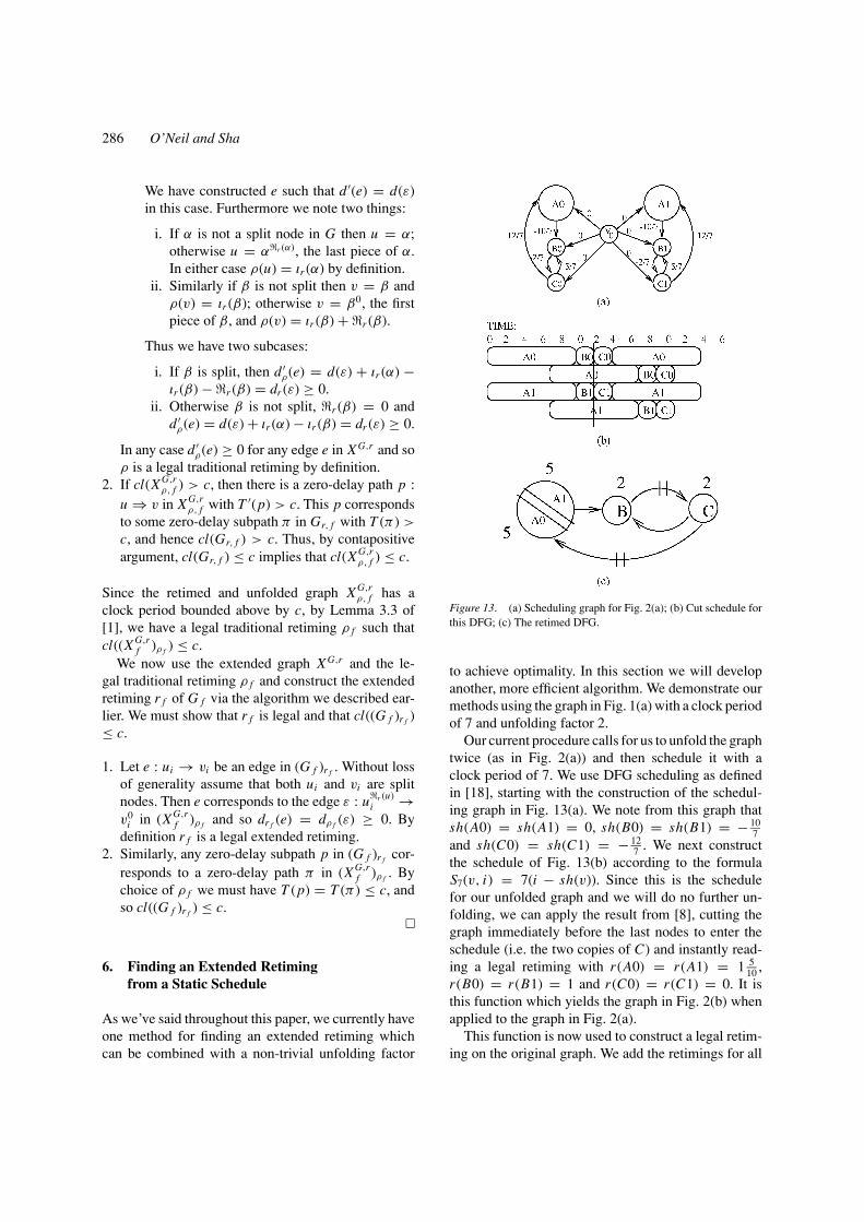
Figure 13. (a) Scheduling graph for Fig. 2(a); (b) Cut schedule forthis DFG; (c) The retimed DFG.

to achieve optimality. In this section we will developanother, more efficient algorithm. We demonstrate ourmethods using the graph in Fig. 1(a) with a clock periodof 7 and unfolding factor 2.

Our current procedure calls for us to unfold the graphtwice (as in Fig. 2(a)) and then schedule it with aclock period of 7. We use DFG scheduling as definedin [18], starting with the construction of the schedul-ing graph in Fig. 13(a). We note from this graph thatsh(A0) = sh(A1) = 0, sh(B0) = sh(B1) = − 10

7and sh(C0) = sh(C1) = − 12

7 . We next constructthe schedule of Fig. 13(b) according to the formulaS7(v, i) = 7(i − sh(v)). Since this is the schedulefor our unfolded graph and we will do no further un-folding, we can apply the result from [8], cutting thegraph immediately before the last nodes to enter theschedule (i.e. the two copies of C) and instantly read-ing a legal retiming with r (A0) = r (A1) = 1 5

10 ,r (B0) = r (B1) = 1 and r (C0) = r (C1) = 0. It isthis function which yields the graph in Fig. 2(b) whenapplied to the graph in Fig. 2(a).

This function is now used to construct a legal retim-ing on the original graph. We add the retimings for all


copies of a particular node together using our special ⊕operator. Thus, for our example, r (A) = 1 5

10 ⊕ 1 510 =

2 + 110 (5, 5), r (B) = 1 ⊕ 1 = 2 and r (C) = 0 ⊕ 0 = 0.

Applying this to our original graph in Fig. 1(a) resultsin the graph in Fig. 13(c), with two delays inside ofnode A next to each other. The result is an optimizedgraph, but the process requires a great deal of time andspace because we are working with the much largerunfolded graph.

In Theorems 4.1 and 5.1, we demonstrated that theorder of application didn’t matter; we could derive anoptimal result either by unfolding then retiming or byapplying retiming first. Therefore, it makes sense thatwe should be able to construct a method similar to theabove one, but which is applied to the original graph.Let us attempt to do what we did above without theunfolding. In other words, we propose to construct ourstatic schedule as before, based on the original graphthis time. We will cut this resulting schedule and readour retiming as before.

We begin by applying this proposed algorithm to thegraph in Fig. 1(a). The scheduling graph with clock pe-riod 7 and unfolding factor 2 is displayed as Fig. 14(a);

Figure 14. (a) Scheduling graph for Fig. 1(a); (b) Cut schedule forthis DFG; (c) The retimed DFG.

note that sh(A) = 0, sh(B) = − 207 and sh(C) = − 24

7in this case. This graph is now scheduled according tothe formula S7/2(v, i) = ⌈

72 (i − sh(v))

⌉and cut before

C’s initial entrance, as in Fig. 14(b). The function thatwe now read has r (A) = 1 + 1

10 (1, 5, 8), r (B) = 1 andr (C) = 0. When applied to the original graph (as inFig. 14(c)), this function appears to be a legal retimingwhich does optimize the graph.

Having established what we want to do, we mustformalize this method and prove its result is a legalretiming which optimizes a DFG. Let S(v, i) = c

f (i −sh(v))� be the integral schedule with clock period cand unfolding factor f . S(v, i) gives the starting timeof node v in the i th iteration. Thus the time at whichthe prologue ends, which we will denote as M and iswhere we want to make our cut, equals the starting timeof the last node to enter the static schedule. In otherwords, M = maxv S(v, 0). (See that M = S(C, 0) = 12above.) We now wish to count the number of eitherwhole or partial occurrences of each node to the left ofthis cut. The i th copy of node v begins to the left ofthe cut if S(v, i) < M . A copy of a node is completeif M − S(v, i) ≥ t(v); otherwise it is partial. Clearlyeach complete copy of a node adds 1 to the eventualretiming function. On the other hand, if a copy is cut,we only want to add the fraction of the node to theleft of the cut, which is found by dividing the piece’scomputation time by the computation time of the wholenode. At the end, we combine the contributions from anode’s copies via our ⊕ operator, finally arriving at theretiming formula

r (v) =⊕

i :S(v,i)<M

min

{1,

M − S(v, i)

t(v)

}. (4)

Since the computation of this formula uses our shortestpath algorithm, it makes sense that it has the same timecomplexity as that algorithm, namely O(|V ||E |). Letus consider this formula when applied to node A ofFig. 1(a). As we can see from our schedule in Fig. 14(b),the first four iterations of A are to be considered whenconstructing the node’s retiming:

1. S(A, 0) = 0 and min{1, 1210 } = 1.

2. S(A, 1) = 72 · 1� = 4 and min{1, 12−4

10 } = 810 .

3. S(A, 2) = 72 · 2� = 7 and min{1, 12−7

10 } = 510 .

4. S(A, 3) = 72 · 3� = 11 and min{1, 12−11

10 } = 110 .

Combining these figures gives us r (A) = 1⊕ 810 ⊕ 5

10 ⊕1

10 = 1+ 110 (1, 5, 8), exactly the same answer we found


by simply examining the schedule table. Our formulaappears to accurately describe this situation.

To further our confidence in this proposition, we canalso check that (4) matches our previous formula from[7, 8], a legal retiming in the case where we have nounfolding. In this case, a simple closed form can bederived.

Lemma 6.1. Let G be a DFG and c a positive integerwith t(v) ≤ c for all nodes v. In the case when f = 1,

Eq. (4) is equivalent to the formula r ′(v) = �sh(v) −X� + min{1, c

t(v) ((sh(v) − X ) − �sh(v) − X�)} whereX = minv sh(v).

Proof: First note that M = −c · X and S(v, i) =c(i − sh(v)) by definition when f = 1. Now, supposethat node v is split in both iterations i and i + k forsome integer k > 0. Since the i th iteration is split, 0 <

M −S(v, i) < t(v), implying that 0 < sh(v)− i − X <t(v)

c ≤ 1 ≤ k. Thus −k < sh(v) − (i + k) − X < 0,and so M − S(v, i + k) < 0. This places the (i + k)thcopy of v as starting after time M , contradicting ourassertion that it was also to be split in our schedule,and we conclude that any node is split in at most oneiteration in the case where f = 1 and t(v) ≤ c for allnodes v.

Given a node v, the only way a copy of v does notappear in the prologue is if M = S(v, 0) and r (v) = 0.

In this case sh(v) = X and r ′(v) = 0 as well. Thisleaves us the case where a copy of v does appear in theprologue, which splits into two subcases:

1. If no copy of v is split, then there exists an integeri > 0 such that M − S(v, i − 1) ≥ t(v) whileS(v, i) − M ≥ t(v). In this case r (v) = i . See thatM − S(v, k) = c(sh(v) − k − X ) for any k, and soM − S(v, i − 1) ≥ t(v) implies that sh(v) − X ≥(i −1)+ t(v)

c . Similarly M −S(v, i) ≤ −t(v) impliesthat sh(v) − X ≤ i − t(v)

c . Since t(v)c ∈ (0, 1], we

thus conclude that �sh(v) − X� = i − 1, and sosh(v)−X−�sh(v)−X� = sh(v)−X−(i−1) ≥ t(v)

c ,or c

t(v) (sh(v) − X − �sh(v) − X�) ≥ 1. Thereforer ′(v) = (i − 1) + 1 = i = r (v).

2. On the other hand assume that the i th copy of v

is split. Therefore M − S(v, i − 1) ≥ t(v) while0 < M−S(v, i) < t(v). See that r (v) = i+ M−S(v,i)

t(v)in this case. Now, M − S(v, i) lying in the interval(0, t(v)) implies that i < sh(v)− X < i + t(v)

c ≤ i +1, so �sh(v)− X� = i . Furthermore, M − S(v, i) =c(sh(v) − i − X ) = c((sh(v) − X ) − �sh(v) − X�),

and so r (v) = �sh(v) − X� + ct(v) ((sh(v) − X ) −

�sh(v) − X�) = r ′(v).

Thus, for all nodes v, r (v) = r ′(v) when f = 1 andt(v) ≤ c for all v.

We now are very confident of our assertion, but muststill show that (4) is, in fact, a legal extended retimingwhich minimizes the iteration period of a data-flowgraph. Recall that these definitions are based on the ır

and r functions for the retiming r in question. There-fore, before proceeding to our primary result, we mustfind the closed forms of these functions for our pro-posed formula.

Lemma 6.2. Let r be the extended retiming given byEq. (4) above. Then ır (v) = � f

c (M − t(v))+sh(v)�+1and r (v) = � f

c (M − 1) + sh(v)� + 1 − ır (v).

Proof:

1. To find the number of complete copies of v in theprologue, we want to find the largest i such thatM − S(v, i) ≥ t(v). This will give us the actualiteration number of the last copy of v in the pro-logue; for the count we must then add 1. Now, sinceS(v, i) = c

f (i − sh(v))� by definition, we see thatthis quantity under the ceiling function is boundedabove by M − t(v), or i ≤ f

c (M − t(v)) + sh(v).Since i must be an integer, we now take the floorfunction of the right-hand side of this inequality tofind the largest possible value for i .

2. Similarly, we must know the iteration number of thefirst copy of v which does not start in the prologue,i.e. the smallest i such that S(v, i) ≥ M . To find thenumber of copies of v that are split in our sched-ule, we then need only subtract ır (v), the number ofcomplete copies of v in our prologue, from i . Now,again by definition of S(v, i), S(v, i) ≥ M impliesthat c

f (i −sh(v)) > M −1 or i >fc (M −1)+sh(v).

If the quantity on the right-hand side of this inequal-ity is not an integer, then we want i equal to theceiling of this quantity, which is the same as thefloor of this quantity plus 1. On the other hand, ifthis quantity is an integer, we must have i equal to1 plus the right-hand side, which is the same as 1plus the floor of the right-hand side. In any casei = � f

c (M − 1) + sh(v)� + 1 and our result isshown.


With this result we can now show:

Theorem 6.3. Let G = 〈V, E, d, t〉 be a DFG withiteration period c

f ≥ 1, i.e. with clock period c andunfolding factor f . Then the retiming r described byEq. (4) is a legal extended retiming on G such thatcl(Gr, f ) ≤ c if and only if the scheduling graph Gs

contains no negative-weight cycle.

Proof:• Assume that cl(Gr, f ) ≤ c. By the known properties

of the iteration bound from [11], we have

B(G) = B(Gr, f )

f≤ cl(Gr, f )

f≤ c

f,

and so T (�)D(�) ≤ c

f for all cycles � in G. Thus W (�) =D(�)− f

c · T (�) ≥ 0 for all cycles � in Gs , and so thescheduling graph contains no negative-weight cycle.

• On the other hand assume that Gs contains nonegative-weight cycle.

1. To prove the legality of r , we must show thatdr (e) = dr (u → v) − r (u) − r (v) = d(e) +ır (u) − ır (v) − r (v) ≥ 0 for any edge e =(u, v) of G. By the definition of the schedulinggraph, sh(v) ≤ sh(u) + d(e) − f

c · t(u), andso d(e) + sh(u) − sh(v) ≥ f

c · t(u). Thus, byLemma 6.2 above,

dr (e) = d(e) + ır (u) − ır (v)

−⌊

f

c(M − 1) + sh(v)

⌋− 1 + ır (v)

= d(e) +⌊

f

c(M − t(u)) + sh(u)

⌋

+ 1 −⌊

f

c(M − 1) + sh(v)

⌋− 1

≥⌊

f

c(1 − t(u)) + (d(e) + sh(u) − sh(v))

⌋

≥⌊

f

c

⌋≥ 0.

2. Let p : u ⇒ v be a path in G with T (p) > c.We wish to show that Dr (p) = D(p) + ır (u) −ır (v) + r (u) ≥ 1. Again, due to the constructionof the scheduling graph, sh(v) ≤ sh(u)+ D(p)−fc (T (p) − t(v)), and so D(p) + sh(u) − sh(v) ≥fc (T (p) − t(v)). Therefore, by Lemma 6.2 again,

Dr (p) = D(p) + ır (u) − ır (v)

+⌊

f

c(M − 1) + sh(u)

⌋+ 1 − ır (u)

= D(p) +⌊

f

c(M − 1) + sh(u)

⌋+ 1

−⌊

f

c(M − t(v)) + sh(v)

⌋− 1

≥⌊

f

c(t(v) − 1)+(D(p)+sh(u) − sh(v))

⌋

≥⌊

f

c(t(v) − 1) + f

c(T (p) − t(v))

⌋

=⌊

f

c(T (p) − 1)

⌋

>

⌊f

c(c − 1)

⌋=

⌊f − f

c

⌋= f − 1

since f ≤ c by assumption. Thus Dr (p) ≥f whenever T (p) > c, and by Theorem 2.2,cl(Gr, f ) ≤ c.

Let’s now summarize what we’ve proven so far:

Theorem 6.4. Let G be a data-flow graph withB(G) ≥ 1 which has no split nodes. Let f and c bepositive integers. The following statements are equiv-alent:1. The iteration bound B(G) ≤ c

f .2. The scheduling graph Gs contains no cycle having

negative delay count.3. There exists a legal extended retiming r on G such

that cy(Gr, f ) ≤ c.4. There exists a legal extended retiming r f on the un-

folded graph G f such that cy((G f )r f ) ≤ c.5. There exists a legal, integral, repeating, static

schedule for G with unfolding factor f and cycleperiod c.

Proof: The equivalence of (1) and (2) is given byLemma 2.3 (Lemma 3.1 of [18]). The equivalence of(2) and (3) is Theorem 6.3 above. The combination ofTheorems 4.2 and 5.1 yield the equivalence of (3) and(4). Finally, the equivalence of (1) and (5) is demon-strated by Theorem 3.5 of [18].

As a final aside, we above raised the question ofexactly how many delays may be placed inside a node.We can now derive our answer in the general case:


Lemma 6.5. Let G be a DFG, with B(G) = cf the

iteration bound in lowest terms. Let k be the smallestpositive integer such that t(v) ≤ kc for all nodes v ofG. Then at most k f delays may be placed inside of anynode as a result of extended retiming.

Proof: Assume by way of contradiction that k f + 1or more delays are to be placed inside of node v. Thisimplies that this many copies of v are cut in the scheduletable. Let i be the smallest iteration number of one ofthese copies, so that 0 < M − S(v, i) < t(v). Byour assumption, the (i + k f )th copy of v is also split,implying that 0 < M − S(v, i + k f ) < t(v). However,S(v, i +k f ) = c

f (i −sh(v)+k f )� = cf (i −sh(v))+

kc� = S(v, i) + kc by definition, and so t(v) ≤ kc <

M − S(v, i), contradicting our choice of i . Thus wemay place at most k f delays within any node v.

Returning to our example in Fig. 1(a), the iterationbound of the graph is 7

2 but the size of node A dictatesthat k = 2. By this lemma, we know that at most 4delays are placed inside any of the three nodes, and thatany node is divided into at most 5 pieces by extendedretiming.

7. Minimum Rate-Optimal Unfolding Factors

As we’ve said, an iteration of a data-flow graph is sim-ply an execution of all nodes once. The average compu-tation time of an iteration is called the iteration periodof the DFG. If the DFG G contains a cycle, the averagecomputation time of the cycle is the total computationtime of the nodes divided by the number of delays inthe cycle. This ratio must be smaller than the iterationperiod of the whole graph since the cycle constitutes asubgraph of G. If we compute the maximum time-to-delay ratio over all cycles of G we derive a lower boundon the iteration period of G. This maximum time-to-delay ratio is called the iteration bound [16] of G andis denoted B(G).

If the iteration period of a graph’s schedule equalsthe graph’s iteration bound, the schedule is said to berate-optimal. As we’ve said throughout this paper, ourgoal is to achieve rate-optimality via retiming and un-folding. If a data-flow graph can be unfolded f timesand achieve rate-optimality (i.e. a clock period equalto f · B(G)), we say that f is the rate-optimal un-folding factor for G. Obviously we wish to achieverate-optimality while unfolding as little as possible. Tothis end we need to compute the minimum rate-optimal

unfolding factor for any graph. We begin by showingthis link between a graph’s clock period and iterationbound:

Lemma 7.1. Let G be a data-flow graph without splitnodes, c a cycle period and f an unfolding factor. Thenthere exists a legal extended retiming r on G such thatcl(Gr, f ) ≤ c if and only if B(G) ≤ c

f .

Proof: By Theorem 5.1, the existence of r impliesthe existence of an extended retiming r f such thatcl((G f )r f ) ≤ c. Note that G f is our unfolded graph;alone it has an unfolding factor of 1. Therefore, by The-orem 2.2 of [7], B(G f ) ≤ c. However, by Property 6.2of [11], B(G f ) = f · B(G) and so B(G) ≤ c

f . Theopposite implication is proved similarly.

With this in hand we can show:

Theorem 7.2. Let G be a data-flow graph withoutsplit nodes. Let � be a critical cycle of G, i.e. B(G) =T (�)D(�) . Let g be the greatest common divisor of T (�) and

D(�). Then D(�)g is the minimum rate-optimal unfolding

factor for G.

Proof: Let σ = T (�)g and ρ = D(�)

g . We need to showthat ρ is a rate-optimal unfolding factor and that it isminimal.

1. By definition B(Gr,ρ) ≤ cl(Gr,ρ) for any retimingr . On the other hand, since B(Gr ) = B(G) for anyretiming r of G,

B(Gr,ρ) = ρ · B(Gr ) = ρ · B(G)

= D(�)

g· T (�)

D(�)= T (�)

g,

which is integral and is thus a legitimate choice ofclock period for G. Since B(Gr,ρ )

ρ= B(G) for any re-

timing r of G, by Lemma 7.1 there exists a legal ex-tended retiming r0 such that cl(Gr0,ρ) ≤ B(Gr0,ρ).Thus cl(Gr0,ρ) = B(Gr0,ρ) and ρ is a rate-optimalunfolding factor by definition.

2. Assume f is any other rate-optimal unfolding factor.Thus there exists an integer c such that B(G) = c

f .Therefore

c

f= σ

ρ= T (�)

D(�),

and so both fractions are reduced forms for B(G).However, by definition of g, σ

ρmust be the most


Table 2. Simulation results for common circuits.

Min. optimal Iter. Pd. w/Computation time unf old factor Bold unf old factor

Benchmark Add Mult Slow-down Iter. Bound Ext. Trad. Ext. Trad.

Second order IIR filter 1 4 2 3 1 2 3 4Second order IIR filter 1 10 6 2 1 6 2 102-Cascaded biquad filter 4 25 6 11

2 2 6 5.5 12.5All-pole lattice filter 2 5 12 3

2 2 6 1.5 2.5All-pole lattice filter 1 12 7 4 1 7 4 12Fifth order elliptic filter 2 12 16 7

2 2 8 3.5 6Fifth order elliptic filter 2 30 20 11

2 2 20 5.5 15

reduced form, and so ρ ≤ f for any other rate-optimal unfolding factor f .

In short, to find the rate-optimal unfolding factor ofa data-flow graph G, we compute B(G) (a polynomial-time operation [19]) and reduce the resulting fractionto lowest terms. The denominator of this fraction is ourdesired unfolding factor.

8. Examples

Let’s consider the data-flow graph representation of aIIR filter. Assume that a multiplier (shown below as acircle) require four units of computation time, as op-posed to one for an adder (shown as a square). Further-more, to complicate our example, multiply the registercount of each edge by 2, referred to in [3] as applyinga slowdown of 2 to our original circuit. The result ispictured in Fig. 15(a).

The resulting circuit has an iteration bound of 3, andcan be retimed via extended retiming to achieve thisclock period as in Fig. 15(b) without unfolding. How-ever, if we restrict ourselves to traditional retiming, thebest clock period we can get is 4. The only way to ob-tain an optimal result is to unfold the graph by a factorof 2 and retime for a clock period of 6, as shown inFig. 15(c).

Repeating this exercise with other common filtersyields Table 2. In all cases, we achieve better resultsby using extended retiming, getting an optimal clockperiod while requiring less unfolding. This improve-ment is illustrated by the last four columns of our table.Limiting ourselves to traditional retiming forces us todecide between two poor options:

Figure 15. (a) A 2-slow second order IIR filter; (b) This graph opti-mized by extended retiming; (c) This graph optimized by traditionalretiming.


1. If we want an optimal clock period we must unfoldby a larger factor, which is listed for each examplein the second-to-last column of Table 2. This dra-matically increases the size of our circuit, and thusthe number of functional units we require and theproduction costs.

2. On the other hand, if we want to unfold by our ex-tended unfolding factor (shown in boldface in thetable), we will be forced to accept a larger iterationperiod (listed in the last column of the same table).The result is a smaller circuit running at less thanoptimal speed.

9. Conclusion

In this paper, we have improved our previous resultby combining extended retiming with unfolding. Wehave shown that the order in which we retime and un-fold is immaterial; this is demonstrated by the com-bination of Theorems 4.1 and 5.1. This result indi-cates that we should be able to find a retiming im-mediately without unfolding first, and we have con-structed an O(|V ||E |) method to do this, based on ourearlier simplified algorithm from [8]. Indeed, we havedemonstrated that our work here is a generalizationof our earlier work [7–10]. We have also proven anupper bound on the number of delays which may beembedded within a node as a result of extended re-timing. Finally, we have developed a method for cal-culating the optimal unfolding factor for extended re-timing: compute the iteration bound, reduce it to low-est terms, then use the denominator of the resultingfraction.

This work represents a theoretical ideal, yieldingthe best possible results while assuming a perfectworld. Moving from this ideal to the real world ofhardware implementations and resource constraintsremains a significant, crucial and complicated nextstep.

In particular, we have developed these resultswhile assuming the use of integral schedules. Wealso have the possibilities of fractional schedules,where operations may be scheduled at any time(not necessarily at integral points) [18]. Addition-ally, we have assumed the use of the most basicdata-flow graph possible, although important varia-tions have been described [20, 21]. We thus have ad-ditional models to explore as we discuss extendedretiming.

Acknowledgments

This work was partially supported by NSF grants MIP-9501006 and MIP-9704276; and by the A.J. SchmittFoundation while the authors were with the Universityof Notre Dame. It was also supported by the Univer-sity of Akron, NSF grants ETA-0103709 and CCR-0309461, Texas ARP grant 009741-0028-2001 and theTI University program.

References

1. L.-F. Chao and E.H.-M. Sha, “Scheduling Data-Flow Graphsvia Retiming and Unfolding,” IEEE Transactions on Paralleland Distributed Systems, vol. 8, 1997, pp. 1259–1267.

2. A. Zaky and P. Sadayappan, “Optimal Static Scheduling of Se-quential Loops on Multiprocessors,” in Proceedings of the In-ternational Conference on Parallel Processing, 1992, pp. III130–137.

3. C.E. Leiserson and J.B. Saxe, “Retiming Synchronous Cir-cuitry,” Algorithmica, vol. 6, 1991, pp. 5–35.

4. S.Y. Kung, J. Whitehouse, and T. Kailath, VLSI and ModernSignal Processing, Prentice Hall, 1985.

5. L.-F. Chao and E.H.-M. Sha, “Retiming and Unfolding Data-Flow Graphs,” in Proceedings of the International Conferenceon Parallel Processing, 1992, pp. II 33–40.

6. M. Lam, “Software Pipelining: An Effective Scheduling Tech-nique for VLIW Machines,” in Proceedings of the ACM SIG-PLAN Conference on Programming Language Design and Im-plementation, 1988, pp. 318–328.

7. T.W. O’Neil, S. Tongsima, and E.H.-M. Sha, “Extended Retim-ing: Optimal Retiming via a Graph-Theoretical Approach,” inProceedings of the IEEE International Conference on Acoustics,Speech and Signal Processing, vol. 4, 1999, pp. 2001–2004.

8. T.W. O’Neil, S. Tongsima, and E.H.-M. Sha, “Optimal Schedul-ing of Data-Flow Graphs Using Extended Retiming,” in Pro-ceedings of the ISCA 12th International Conference on Paralleland Distributed Computing Systems, 1999, pp. 292–297.

9. T.W. O’Neil and E.H.-M. Sha, “Rate-Optimal Graph Transfor-mation via Extended Retiming and Unfolding,” in Proceedingsof the IASTED 11th International Conference on Parallel andDistributed Computing and Systems, vol. 10, 1999, pp. 764–769.

10. T.W. O’Neil and E.H.-M. Sha, “Optimal Graph Transformationusing Extended Retiming with Minimal Unfolding,” in Proceed-ings of the IASTED 12th International Conference on Paralleland Distributed Computing and Systems, 2000, pp. 128–133.

11. K.K. Parhi and D.G. Messerschmitt, “Static Rate-OptimalScheduling of Iterative Data-Flow Programs via Optimum Un-folding,” IEEE Transactions on Computers, vol. 40, 1991,pp. 178–195.

12. P.-Y. Calland, A. Darte, and Y. Robert, “Circuit Retiming Ap-plied to Decomposed Software Pipelining,” IEEE Transactionson Parallel and Distributed Systems, vol. 9, 1998, pp. 24–35.

13. F. Sanchez and J. Cortadella, “Reducing Register Pressure inSoftware Pipelining,” Journal of Information Science and Engi-neering, vol. 14, 1998, pp. 265–279.


14. K.S. Chatha and R. Vemuri, “RECOD: A Retiming Heuris-tic to Optimize Resource and Memory Utilization in HW/SWCodesigns,” in Proceedings of the IEEE International Workshopon Hardware/Software Codesign, 1998, pp. 139–143.

15. M. Sheliga, N.L. Passos, and E.H-M. Sha, “Fully Parallel Hard-ware/Software Codesign for Multi-Dimensional DSP Applica-tions,” in Proceedings of the IEEE International Workshop onHardware/Software Codesign, 1996, pp. 18–25.

16. M. Renfors and Y. Neuvo, “The Maximum Sampling Rate ofDigital Filters Under Hardware Speed,” Transactions on Circuitsand Sampling, vol. CAS-28, 1981, pp. 196–202.

17. L.-F. Chao, “Scheduling and Behavioral Transformations forParallel Systems,” PhD thesis, Dept. of Computer Science,Princeton University, 1993.

18. L.-F. Chao and E. H.-M. Sha, “Static Scheduling for Synthesisof DSP Algorithms on Various Models,” Journal of VLSI SignalProcessing, vol. 10, 1995, pp. 207–223.

19. A. Dasdan and R.K. Gupta, “Faster Maximum and MinimumMean Cycle Algorithms for System-Performance Analysis,”IEEE Transactions on Computer-Aided Design of IntegratedCircuits and Systems, vol. 17, 1998, pp. 889–899.

20. E.A. Lee and D.G. Messerschmitt, “Static Scheduling of Syn-chronous Data-Flow Programs for Digital Signal Processing,”IEEE Transactions on Computers, vol. 36, 1987, pp. 24–35.

21. G. Bilsen, M. Engels, R. Lauwereins, and J. Peperstraete,“Cyclo-Static Dataflow,” IEEE Transactions on Signal Process-ing, vol. 44, 1996, pp. 397–408.

Timothy O’Neil received his Ph.D. in Computer Science and Engi-neering from the University of Notre Dame in 2002, where he was

awarded the Arthur J. Schmitt Fellowship. He also received master’sdegrees in mathematics (1991) and computer and information sci-ences (1993) from The Ohio State University in Columbus, Ohio.He is presently an Assistant Professor in the Computer Science De-partment at the University of Akron. His current research interestsinclude loop transformations and data scheduling.

Edwin Hsing-Mean Sha received the B.S.E. degree in computerscience and information engineering from National Taiwan Univer-sity, Taipei, Taiwan, in 1986; he received the M.A. and Ph.D. degreefrom the Department of Computer Science, Princeton University,Princeton, NJ, in 1991 and 1992, respectively. From August 1992to August 2000, he was with the Department of Computer Scienceand Engineering at University of Notre Dame, Notre Dame, IN. Heserved as Associate Chairman for Graduate Studies from 1995 to2000. Since 2000, he has been a tenured full professor in the Depart-ment of Computer Science at the University of Texas at Dallas.

He has published more than 170 research papers in referred con-ferences and journals. He has been serving as an editor for severaljournals such as IEEE Transactions on Signal Processing and Journalof VLSI Signal Processing. He also served as program committeemembers in numerous conferences. He received Oak Ridge Associa-tion Junior Faculty Enhancement Award in 1994, and NSF CAREERAward. He was a guest editor for the special issue on Low Power De-sign of IEEE Transactions on VLSI Systems in 1997. He also servedas the program chairs for the International Conference on Paralleland Distributed Computing Systems (PDCS), 2000 and PDCS 2001.He received Teaching award in 1998.

Combining Extended Retiming and Unfolding for Rate …toneil/research/papers/journals/jvsp05.pdf ·...

Documents

Transcript of Combining Extended Retiming and Unfolding for Rate …toneil/research/papers/journals/jvsp05.pdf ·...