ORIGINAL PAPER

Combined Scaling of Fluid Flow and Seismic Stiffnessin Single Fractures

C. L. Petrovitch • L. J. Pyrak-Nolte •

D. D. Nolte

Received: 4 April 2014 / Accepted: 10 April 2014

� Springer-Verlag Wien 2014

Abstract The connection between fluid flow and seismic

stiffness in single fractures is governed by the geometry of

the fracture through the size and spatial distributions of the

void and contact areas. Flow and stiffness each exhibit

scaling behavior as the scale of observation shifts from

local to global sample sizes. The purpose of this study was

to explore the joint scaling of both properties using

numerical models. Finite-size scaling methods are used to

extract critical thresholds and power laws for fluid flow

through weakly correlated fractures under increasing load.

An important element in the numerical fracture deforma-

tion is the use of extended boundary conditions that sim-

ulate differences between laboratory cores relative to

in situ field studies. The simulated field conditions enable

joint scaling of flow and stiffness to emerge with the

potential to extrapolate from small laboratory samples to

behavior on the field scale.

Keywords Hydromechanical scaling � Scaling � Fracture

deformation � Rock fractures � Fracture

1 Introduction

The mechanical and hydraulic properties of a fracture

depend on the morphology of rough surfaces. For example,

fluid flow through a fracture depends on the size and spatial

distribution of the apertures that are formed by placing two

rough surfaces in contact (Brown 1989; Brown et al. 1995;

Engelder and Scholz 1981; Lomize 1951; Neuzil and Tracy

1981; Pyrak-Nolte et al. 1987, 1988; Renshaw 1995; Tsang

1984; Tsang and Tsang 1987; Watanabe et al. 2008;

Witherspoon et al. 1980). On the other hand, other studies

have shown that fracture displacement depends on the

surface roughness and the spatial distribution of contact

area within a fracture (Bandis et al. 1983; Barton et al.

1985; Brown and Scholz 1985; Hopkins 1990; Hopkins

et al. 1990; Kendall and Tabor 1971; Swan 1983; Yoshioka

and Scholz 1989). Thus, it is plausible that through the

properties of rough surfaces, their contact and their

deformation, that a relationship between fluid flow through

a fracture and fracture stiffness could exist (Cook 1992;

Pyrak-Nolte 1996; Pyrak-Nolte and Morris 2000). How-

ever, prior to Petrovitch et al. (2013), no simple relation-

ship had been determined because the mechanical and

hydraulic properties depend on fracture geometry in dif-

ferent ways. Flow through a fracture is dominated by the

dependence on the aperture distributions (both in size and

in spatially), while fracture closure and fracture-specific

stiffness depend primarily on the contact areas (Hopkins

et al. 1990; Jaeger et al. 2007). These factors indicate that,

while a fracture is under a normal load, flow requires

geometric quantities beyond mean aperture to describe the

system fully.

Witherspoon et al. (1980) conducted an experimental

study to validate the cubic law for fractures under normal

load. The cubic law is the solution to the Navier–Stokes

C. L. Petrovitch (&)

Applied Research Associates Inc., Raleigh, NC, USA

e-mail: cpetrovitch@gmail.com

L. J. Pyrak-Nolte � D. D. Nolte

Department of Physics, Purdue University, West Lafayette, USA

L. J. Pyrak-Nolte

School of Civil Engineering, Purdue University,

West Lafayette, USA

L. J. Pyrak-Nolte

Department of Earth, Atmospheric and Planetary Sciences,

Purdue University, West Lafayette, USA

123

Rock Mech Rock Eng

DOI 10.1007/s00603-014-0591-z

equation for flow between horizontal parallel plates with

dimensions w and L, and separated by a distance h (the

aperture). The cubic law is written as follows:

q ¼ �wh3

12loP

oxð1Þ

where w is the width of the channel, l is the fluid viscosity,

and qp/qx is the pressure gradient over the length of the

fracture, L. In Eq. (1), flow depends on the cube of the

aperture. Thus, as stress is applied to a fracture, and the

mean aperture decreases, flow through a fracture decreases.

In their experiment, Witherspoon et al. made measure-

ments of fluid flow as a function of normal load while loading

and unloading a tensile fracture in marble. In their work, they

determined that the cubic law holds for low stresses when the

mean aperture is large and the relative roughness is small. At

high stress, they observed deviations from the cubic law.

Zimmerman et al. (1990) and Zimmerman and Bodvarsson

(1996) attributed deviations from cubic law to the condition

when the dominant surface roughness wavelength is

approximately equal to the hydraulic aperture. While Ren-

shaw (1995) noted that the deviation from cubic law

behavior occurred when the standard deviation in aperture

remained nearly constant as the normal stress increased. The

roughness and mean aperture play a vital role in fluid flow

through a fracture, and Walsh (1981) used the solution for the

flow through a channel with a circular blockage of radius

a. This allowed the effects of contact to be included in the

hydraulic aperture rather than the surface roughness. Thus,

the combination of the decreasing mean aperture, increasing

relative roughness, and increasing contact area allows fluid

flow to change differently than the cube of the mean aperture.

At high stresses, Pyrak-Nolte et al. (1987, 1988) found

that the exponent deviated from cubic law and observed

values as high as 8–10. In this study, metal casting of the

void spaces of natural fractures in granite was made under

normal loads as high as 85 MPa. Cook (1992) described

the void geometries at large stresses; ‘‘the existence of

large oceanic regions of open fracture, [are] connected by

tortuous paths through archipelagic’ regions filled with

numerous small, closely spaced contact regions’’. Pyrak-

Nolte et al. concluded that as the stress increased, the large

oceanic regions continued to deform, decreasing the mean

aperture, while the small tortuous paths (that connect each

larger region) controlled the flow. Since the small tortuous

paths have relatively large aspect ratios (aperture height to

channel width), the local stiffness was extremely large.

Therefore, at large stresses, the flow rate is approximately

stress independent while the mean aperture is not.

From the metal casting experiments (Pyrak-Nolte et al.

1987), Pyrak-Nolte (1996) hypothesized that an understand-

ing of both the underlying void and contact geometries is

required to explain the deviation from the cubic law. Pyrak-

Nolte and Morris (2000) conducted numerical simulations to

investigate the effect of the geometry of the fracture on the

relationship between fluid flow and fractures stiffness. Using

laboratory data from Witherspoon et al. (1980), Raven and

Gale (1985), Gale (1982, 1987), and Pyrak-Nolte et al. (1987),

the flow rates and stiffness were plotted parametrically. It was

observed that within this data set, several of the flow rates for

fractures did not vary considerably as a function of stiffness,

while others decreased several orders of magnitude as the

stiffness increased. From their computational efforts, Pyrak-

Nolte and Morris (2000) attributed these differences to the

spatial correlation length of the fracture void geometry. For

their simulations, they used two types of fractures: those with

short correlation lengths (random geometries) and those with

long correlation lengths (large ‘‘oceanic’’ regions). After

averaging fractures of each type, it was concluded that the

flow–stiffness relationship is dependent on the correlation

length of the void space geometry. Fractures with short-range

correlation lengths maintained multiple flow paths that con-

tinued to support flow as the normal stress on the fracture

increased. On the other hand, highly correlated fractures were

composed of only one or two dominant flow paths that rapidly

closed with increasing load and resulted in a rapid decrease in

flow with increasing fracture-specific stiffness.

The work of Pyrak-Nolte and Morris (2000) demon-

strated that fracture void geometry is the link between fluid

flow and fracture-specific stiffness. In this paper, we

present results of a numerical study that uses finite-size

scaling to demonstrate the existence of a combined scaling

relationship between fluid flow and fracture-specific

stiffness.

2 Fracture Model

The relationship between fluid flow and fracture-specific

stiffness is based on the assumption that these two fracture

properties are implicitly linked through the fracture

geometry (Pyrak-Nolte 1996; Pyrak-Nolte and Morris

2000). When two rough surfaces are brought together,

regions of contact between the surfaces are formed as well

as void with variable shape and aperture. Fracture geom-

etry includes the probability and spatial distributions of

both the contact area between the two fracture surfaces and

the aperture distribution. Many methods have been used to

generate fracture void geometry. Many numerical approa-

ches simulate void geometries by generating two self-affine

or self-similar rough surfaces that are then brought into

contact to form the void geometry (Borodich and Onis-

hchenko 1999; Glover et al. 1998; Peitgen and Saupe 1988;

Walsh 1965). In this study, fracture geometry was gener-

ated by creating void spaces directly, rather than two rough

surfaces, using a random 2D continuum percolation

C. L. Petrovitch et al.

123

approach. The 2D continuum percolation approach pro-

vides synthetic fractures with log-normal aperture distri-

butions and tunable correlation lengths. The percolation

properties and fractal behavior of the synthetic fractures

have been extensively studied (Nolte et al. 1989; Nolte and

Pyrak-Nolte 1991, 1997; Pyrak-Nolte et al. 1992).

Fracture void geometry was created by randomly filling

an initially zeroed 512 9 512 array by a selected number of

points (NPTS). A point is defined by a point size which for

this study was a 4 9 4 subarray (point size = 4). When a

point is randomly plotted in the array, each array element is

incremented by one. This increment in aperture as the points

are plotted results in an aperture distribution. An example of

the void geometry for a fracture with apertures with a short

correlation length is shown in Fig. 1 (left). In this study, only

weakly correlated fractures were generated. Each fracture

has NPTS = 37,726 to achieve an initial void fraction of

approximately 95 %. At the 512 9 512 scale, the fracture

has an edge length of 1.0 m. A single point or pixel has an

edge length of 1.95 mm. A point size = 4 results in a spatial

correlation length of 7.8 mm (the grain size) and a log-nor-

mal aperture distribution (Fig. 1, right).

All fractures were generated on the 512 9 512 (1 m)

scale and then subsectioned to study the scaling properties

of fluid flow, fracture displacement, and fracture-specific

stiffness. The subsections ranged from 256 9 256 down to

32 9 32, resulting in scales from 1, �, �, 1/8, 1/16, and

1/32 of the original 512 9 512 pattern. Fluid flow and

fracture deformation were calculated (using the numerical

methods discussed in the following sections) for 100

fractures at each scale.

3 Deformation Model

3.1 The Hopkins Model

To determine the specific stiffness for a fracture, it is

necessary to calculate fracture deformation by including

the superposition of all far-field displacements in response

to all the asperities as a function of stress. In this study,

fractures were deformed numerically under a normal load

using a method similar to that developed by Hopkins

(1990). Hopkins approach assumes that a fracture can be

approximated by two parallel half-spaces separated by an

asperity distribution. This assumption is similar to Green-

wood and Williamson’s model (1966) where the joint was

represented as an asperity distribution in contact with a flat

and rigid surface, with later improvements by Brown and

Scholz (1985) where a fracture was modeled as two rough

surfaces in contact. Unlike these methods, Hopkins

approach included the interaction between contact points

by allowing each of the half-spaces to deform about the

asperities in addition to and in response to the deformation

of the asperity. No interpenetration of the two rough sur-

faces is allowed. This section provides a detailed descrip-

tion of the deformation model in the spirit of Hopkins

(1990) and Pyrak-Nolte and Morris (2000).

In this approach, each asperity in the fracture is repre-

sented as a cylinder arranged on a regular lattice. Cylinders

are used instead of the common Hertzian approach of two

spheres in contact because the Hertzian solution is only

valid when the radius of a contact is small compared with

the radius of the sphere, it only gives compression of the

tips of the asperities and it neglects the contribution to the

deformation from the half-spaces. Hopkins (2000) showed

that only 5 % of the total normal displacement at an iso-

lated asperity is from compression of the asperity. The

remainder of the displacement is from deformation of the

half-spaces. In Hopkins (2000) approach, the increase in

contact area with stress arises from the increase in the

number of contacting asperities and contributes more to the

increase in contact area than the deformation of the

asperity tip in the Hertzian approach.

For each asperity, the height of a cylinder is determined

by the fracture generation model (see Sect. 2) and is given

a radius, a, such that all cylinders are initially in contact

with their neighboring cylinders (Fig. 2, left). When a load

Fig. 1 Left: example of a

spatially uncorrelated fracture

void geometry. The color

represents the size of the

aperture. Right: histogram of

the log-normal aperture

distribution shown in the left

(color figure online)

Combined Scaling of Fluid Flow and Seismic Stiffness in Single Fractures

123

is applied, the model deforms the half-spaces about the

asperities (Fig. 2, right) and deforms the asperities due to

the contact force of the half-spaces. The deformation of an

asperity is given by

Wi ¼ wii þX

i 6¼j

wij ð2Þ

where Wi is the total deformation at asperity i, and wij is the

deformation at asperity i due to the deformation caused by

asperity j. By allowing the half-spaces to deform, the total

deformation at each asperity is a superposition of the self-

interaction (displacement caused by the half-space, which

is the first term in Eq. 2) and the asperity–asperity inter-

action (displacements caused by the deformation of the

half-spaces via all other asperities, which is the second

term in Eq. 2). The interaction displacement term is what

differentiates Hopkins model from other approaches. For

this study, the cylinders were given the physical properties

of granite: Young’s modulus, E = 60 GPa and Poisson’s

ratio, n = 0.25.

The deformation of the half-space was calculated using

the Boussinesq solution for the normal deformation of a

half-space under a uniformly loaded circle (Timoshenko

and Goodier 1970). For points beneath the loaded circle

(r B a), the deformation is given by

wi r� að Þ ¼ 4 1� v2ð Þqa

pE

Zp2

0

1� r2

a2sin2 h dh; ð3Þ

while the deformation for locations outside the circle

(r [ a) is given by

wo r [ að Þ ¼ 4 1� v2ð Þqa

pE

�Zp

2

0

1� a2

r2sin2 h dh� 1� a2

r2

� �Zp2

0

dh

1� a2

r2 sin2 h

264

375 ð4Þ

where q is the stress at each asperity and is equal to f/(pa2);

f is the force on an asperity. The average displacement, dij,

is determined by finding the total displacement at each

asperity, i, caused by the force at j which is found by

integrating Eqs. 3 and 4 over the entire area of the fracture,

A, and dividing by the area of a single asperity:

dij ¼1

pa2

ZZ

A

wo r;Cð Þdrdh ð5Þ

where C is the set of asperities in contact. The total dis-

placement, Wi, at asperity i caused by the deformation of

all of the asperities is found by summing the average dis-

placement caused by all of the asperities:

Wi ¼X

j2C

dij ð6Þ

where C is the set of asperities in contact. The stress also

results in the deformation of the asperity. The displacement

of asperity i under a compressive load, f, is

Dhi ¼fihi

pa2Eð7Þ

where hi is the initial height of asperity i, and fi is the force

at asperity i. The force exerted by a given asperity depends

on the displacement of the half-spaces. In turn, the dis-

placement of the half-spaces depends on the forces exerted

by all of the other asperities. A system of linear equations

is formed by recognizing that the initial sum of the dis-

tances between the half-spaces in the absences of asperities

(D in Fig. 2) and the total deformation, Wi, must be equal

to the length of the asperity

DþWi ¼ hi � Dhi ð8Þ

Equation 8 represents a system of simultaneous linear

equations in terms of Dhi because Wi depends indirectly on

Dhi through the force term in Eq. 7. The resulting system is

large (N2 9 N2, where N is the number of asperities in

contact), dense and computationally intensive to solve

directly as it would require O(N4) operations. The conju-

gate gradient method was chosen to solve this system of

linear equations because it reduces the problem to a

matrix–vector multiplication. The computation time for the

solver was reduced by recognizing that long-range inter-

actions can be approximated accurately by performing a

Taylor series expansion around the half-space’s displace-

ment for large radii. Using this approximation, the matrix–

vector product can be rapidly calculated using the fast

multipole method (FMM) (Pyrak-Nolte and Morris 2000).

Additional details on the implementation of the FMM can

be found in Petrovitch (2013).

The fracture-specific stiffness is calculated from the

displacement–stress curve generated by the deformation

models. The stiffness is defined as

jðrÞ ¼ drdd

ð9Þ

Fig. 2 Left: deformation model aligns the standing cylinders along a

lattice-grid. The shades of gray represent different asperity heights.

Right: an illustration of the half-spaces deforming around the

asperities

C. L. Petrovitch et al.

123

where r is the stress applied to the fracture and d is the

average displacement of the fracture given by

di ¼Do � D�Wi if not in contact

Do � hi � Dhi if in contact

�

d ¼X

i

di

Nfor N asperities in contact

ð10Þ

where Do is the zero-stress spacing between the half-spaces

(Fig. 2)

3.2 The Importance of Boundary Conditions

The approach described above computes the fracture

deformation as a function of stress for the condition of free

boundaries. This is similar to the conditions in the laboratory

when a finite sample, like a core, is placed under a constant

displacement load. Contact points near the edges have less

support than those near the center, leading to a non-uniform

closure. This is fundamentally different from what would be

found in the field. Field measurements of fracture-specific

stiffness using remote seismic methods would probe local

parts of a larger fracture. For this reason, periodic boundary

conditions (PBC) were used to simulate conditions similar to

the field by introducing an ‘‘external’’ lattice of multipole

moments in the FMM calculation (Lambert 1994).

Adding PBC to a system of interacting bodies (contact

points in this case) requires detailed consideration. The

system must be repeated infinitely in both the x and

y directions. The system could simply be copied for a finite

distance in each direction to approximate the infinite case,

but, in using this method, the number of bodies grows too

quickly to calculate. There are two common methods to

overcome this: Ewald summations (Schmidt and Lee 1991)

and the macroscopic expansion (ME) (Lambert 1994). In

our work, the macroscopic expansion method was used

because it reuses the FMM formalism already in place. The

macroscopic expansion method begins by assuming the

system is repeated according to a regular rectangular lat-

tice, where each lattice point is a copy of the system of

interacting bodies. Using the FMM formalism, the multi-

pole moments of the system can be used at each lattice

point, instead of directly copying the system.

For the macroscopic expansion method to work, three

modifications were made to the standard FMM algorithm.

First, the top level in the quad-tree must ‘‘feel’’ the effect of

the lattice, thereby enabling the method to overcome the

need to directly sum each lattice point. Second, the inter-

action lists of any given region must wrap periodically to

the opposite side of the domain. Third, the direct sum of the

interacting bodies at the highest resolution must wrap

periodically to their near neighbors. Petrovitch (2013)

gives a complete description of the equations and imple-

mentation of the macroscopic expansion method.

With the three modifications in place, the formalism of the

ME method approximates PBC when deforming the fracture

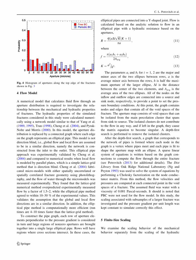
plane. Figures 3 and 4 provide a comparison of the effect of

assuming PBC versus free boundary conditions. In Fig. 3, the

aperture distribution of a fracture subjected to 10 MPa of

normal stress is shown after normalizing by the initial

unstressed aperture distribution. When a fracture is subjected

to free boundary conditions, the fracture preferentially

deforms around the perimeter of the fracture plane (Fig. 3a).

The final perimeter apertures are a small fraction of the initial

values, while the central apertures closed the least. The

deformation is more uniform when PBC are used. Figure 4 is a

histogram of the apertures taken from the top edge (or row) of

the fractures shown in Fig. 3. The free boundary conditions

cause greater deformation along the edge of the sample than

the PBC. The histogram shows that the deformed fracture

under free boundary conditions has significantly more small

apertures along the edge. As will be shown in the next section,

preferential closure of the apertures near the perimeter of the

fracture strongly affects the percolation properties.

Fig. 3 Comparison of

normalized aperture (black)

distribution for a free boundary

conditions and b PBC. The

aperture distributions were

normalized by the aperture

distribution for the same

fracture under no load

Combined Scaling of Fluid Flow and Seismic Stiffness in Single Fractures

123

4 Flow Model

A numerical model that calculates fluid flow through an

aperture distribution is required to investigate the rela-

tionship between the mechanical and hydraulic properties

of fractures. The hydraulic properties of the simulated

fractures considered in this study were calculated numeri-

cally using a network model similar to that of Yang et al.

(1989, 1995), Tran (1998), Cheng et al. (2004), and Pyrak-

Nolte and Morris (2000). In this model, the aperture dis-

tribution is replaced by a connected graph where each edge

on the graph represents an elliptical pipe. This model is not

direction blind, i.e., global flow and local flow are assumed

to be in a similar direction, namely the network is con-

structed from the inlet to the outlet. This elliptical pipe

approach was experimentally validated by Cheng et al.

(2004) and compared to numerical results when local flow

is modeled by parallel plates, which is a simple lattice-grid

method that is direction blind. Cheng et al. (2004) fabri-

cated micro-models with either spatially uncorrelated or

spatially correlated fracture geometry using photolithog-

raphy, and the flow of water through the micromodels was

measured experimentally. They found that the lattice-grid

numerical method overpredicted experimentally measured

flow by a factor of 1.5–2, while the elliptical pipe method

agreed to within 10–30 % of the experimental values. This

validates the assumption that the global and local flow

directions are in a similar direction. In addition, the ellip-

tical pipe method is computationally more efficient (run

times are 4–10 times faster than the lattice-grid method).

To construct the pipe graph, each row of aperture ele-

ments perpendicular to the pressure gradient is considered

in turn and large regions of nonzero apertures are brought

together into a single large elliptical pipe. Rows will have

regions where cross sections intersect. In these cases, the

elliptical pipes are connected into a Y-shaped joint. Flow is

calculated based on the analytic solution to flow in an

elliptical pipe with a hydraulic resistance based on the

apertures,

R ¼ 4f lDlffiffiffiffiKp

K þ 1ð Þpa

; ð11Þ

where

f ¼ p a1b1 þ a2b2ð Þ2Aavg

; ð12Þ

K ¼ a2�h2: ð13Þ

The parameters ai and bi for i = 1, 2 are the major and

minor axes of the two ellipses between rows, a is the

average minor axis between the rows, h is half the maxi-

mum aperture of the larger ellipse, Dl is the distance

between the center of the two elements, and Aavg is the

average area of the two ellipses. All of the nodes on the

inflow and outflow edges are connected into a source and

sink node, respectively, to provide a point to set the pres-

sure boundary conditions. At this point, the graph contains

nodes and edges that contain all of the void spaces of the

fracture. The aperture map consists of void spaces that can

be isolated from the main percolation cluster that spans

from sink to source. The isolated clusters do not contribute

to the flow in any way, and if left in the graph, they cause

the matrix equation to become singular. A depth-first

search is performed to remove the isolated clusters.

After the depth-first search, a graph that corresponds to

the network of pipes is formed where each node in the

graph is a vertex where pipes meet and each pipe is fit to

shape the aperture map with an ellipse. A sparse linear

system of equations is written based on the graph con-

nections to compute the flow through the entire fracture

(see Petrovitch (2013) for additional details). The Dist

Library from Oak Ridge National Laboratory (Ng and

Peyton 1993) was used to solve the system of equations by

performing a Cholesky factorization on the node conduc-

tance matrix. From this method, the flow velocities and

pressures are computed at each connected point in the void

spaces of a fracture. The assumed fluid was water with a

viscosity of 0.001 Pascal-seconds. It should is noted that

PBC were not used for the flow model. In this study, the

scaling associated with subsamples of a larger fracture was

investigated and the pressure gradient per unit length was

kept constant to simulate correctly this effect.

5 Finite-Size Scaling

We examine the scaling behavior of the mechanical

behavior separately from the scaling of the hydraulic

Fig. 4 Histogram of apertures along the top edge of the fractures

shown in Fig. 3

C. L. Petrovitch et al.

123

properties of a fracture in the first section before addressing

the joint scaling relationship between these two fracture

properties.

5.1 Concept of Critical Scaling

The concept of critical scaling comes from the statistical

mechanics of phase transitions like the percolation transi-

tion in fluid flow. When measuring the properties of a

system in a critical regime, properties become scale

dependent. In general, a physical property, v, that scales

critically follows the functional form

v / L�a=lF p� pcð ÞL1=lh i

ð14Þ

where L is the scale of the system, p is the occupation

probability, pc is the critical probability, l is the correlation

exponent, and a is the critical exponent associated with the

property v. F is called a universal function that is specific

to the process and is valid at all scales. Since the generated

fractures are weakly correlated, the occupation probability

(of any given cell) cannot be explicitly defined. However,

this was overcome by considering the average probability

that a given cell is occupied, i.e., the void area fraction.

When studying flow rates, q, through fractures, Eq. 14 is

rewritten as

q / L�t=lF Af � Acð ÞL1=lh i

ð15Þ

where t is the transport exponent, and Af and Ac are the

void area fraction and critical void area fraction, respec-

tively. The important aspect of Eq. 15 is that at threshold

(Af - Ac = 0), the universal function reduces to a constant

and the flow rate is dominated by the observation scale

L raised to the exponent -t/l. Writing flow in this form

allows the transport exponent and the universal function to

be computed numerically.

A Monte Carlo simulation was performed using the

fracture generation, fracture deformation and the flow

models discussed earlier. First, a spanning probability

analysis as a function of scale was performed on weakly

correlated aperture distributions subjected to normal load-

ing for the free and for the PBC. The spanning probability

is the probability that a connected void path exists across

the entire length of the fracture. This analysis illuminates

the critical scaling regimes (if they exist) and critical

threshold with respect to the deformation of the void

spaces. Figure 5a and b shows the spanning probability for

the five scales used in this study for both the free and the

PBC. When a fracture is deformed under the free boundary

conditions, no clear threshold in the flow is observed

(Fig. 5a). The threshold appears to shift with scale. The

free boundary conditions fail to produce a scaling system

because one of the main assumptions in scaling theory is

that, when dealing with a system of scale L, the moments of

any subsample of scale, L0 = L/b, are independent of the

location from which the subsamples were taken. Yet in the

case of the free boundary conditions, subsections taken

from near the edges of the sample have higher contact areas

than those taken from the center. Therefore, the threshold

for free boundary conditions is dominated by edge effects.

However, when the PBC are used, a scaling behavior is

observed with a clear scale-invariant fixed point. Using

renormalization theory, the critical threshold at infinite

scale was determined to be Ac = 0.56. Based on this

(a) (b)

Fig. 5 Spanning probability as a function void area fraction showing the finite-size scaling of percolation threshold when a free boundary

conditions and b PBC are used

Combined Scaling of Fluid Flow and Seismic Stiffness in Single Fractures

123

analysis, only the fractures deformed using the periodic

boundary condition are used in the study of the scaling of

the fluid flow–fracture-specific stiffness relationship.

5.2 Fracture-Specific Stiffness

At each scale, an initial unstressed aperture distribution

was deformed numerically under a normal load. The

average displacement vs. stress curve was generated based

on 100 fracture patterns and was used to extract fracture-

specific stiffness. Figure 6 shows the fracture-specific

stiffness scaled by L/L0 (subsection observation scale

divided by the original scale of the fracture) as a function

of contact area for the five scales used in this study. When

either the free boundary conditions (Fig. 6a) or the PBC

(Fig. 6b) are used, there is no critical scaling, but the cal-

culated fracture stiffnesses for all scales lie on a single

curve. Conceptually, this is much simpler than in the case

of fluid flow. For fluid flow, the critical threshold occurs

when a fracture no longer supports flow. The analogous

property for fracture stiffness is the force that is transmitted

through the fracture (normal to the fracture plane). The

threshold is immediately realized when there is no contact

between the two rough surfaces. Under this condition, no

force can be transmitted through the fracture, thereby set-

ting the fracture-specific stiffness to zero. As soon as points

come into contact, the fracture resists deformation, leading

to a nonzero stiffness. While the assumed boundary con-

ditions had a profound effect on the spanning probability

behavior, it was not as critical for calculating fracture-

specific stiffness. As for the spanning probability, the

scaled fracture-specific stiffness is plotted as a function of

the contact area fraction in Fig. 6. It is observed that there

is no critical scaling for both boundary conditions, only

simple scaling by the ratio of the observation scales. The

fractures in this study contain only short-range correlations,

and the dependence of stiffness on length of the fracture is

a simple proportional relationship. In the work of Morris

(2012) and Morris et al. (2013), the fracture generation

included longer-range correlations, and they found that the

dependence of fracture-specific stiffness on scale differed

from a simple proportionality.

5.3 Scaling of Hydromechanical Coupling

The previous sections described the thresholds for fracture-

specific stiffness and the spanning probability. In this

section, we present the scaling behavior of the coupled

system, i.e., the flow–stiffness relationship. Only fractures

simulated using PBC are considered because free boundary

conditions do not generate fractures with a well-defined

scaling threshold. For each scale, 100 fracture aperture

distributions were stressed, numerically, to a load of

75 MPa in approximately 80 stress increments. For each

increment in stress, the permeability was recomputed. The

fluid flow finite-size scaling relationship (Eq. 15) is

rewritten as

q / L�t=lF Af rð Þ � Ac rð Þð ÞL1=lh i

ð16Þ

where the only difference between Eqs. 15 and 16 is that in

Eq. 16, the area fraction is a function of stress, r. Flow

values were chosen at threshold and plotted against their

respective scales to extract the flow exponent. A power law

fit to the data yielded the exponent t/l = 2.4. The scaled

permeability is shown in Fig. 7. The permeability is scaled

by a simple scaling (L/a3 where a is the mean aperture for

(a) (b)

Fig. 6 Scaled fracture-specific stiffness as a function of contact area for a range of fracture sizes is shown when the computation is performed

using a free boundary conditions and b PBC. Fracture-specific stiffness is scaled by the ratio of L/L0

C. L. Petrovitch et al.

123

the fracture at zero stress) and by critical scaling Lt/l. There

is a fixed point above which flow increases with increasing

size of the fracture and below which flow decreases with

increasing fracture size.

In Fig. 8, scaled permeability is graphed as a function of

fracture-specific stiffness. The flow–stiffness data are par-

tially collapsed by scaling the flow rate by (L/L0)t/l, i.e.,

reflecting the prefactor of the universal scaling function in

Eq. 16. Note that L has been replaced by the non-dimen-

sional value L/L0, where L0 is the largest length used (1 m),

and q contains the same simple scaling (L/a3) used in Fig. 7.

This scaling also displays a fixed point near 5,800 MPa/mm,

where each of the flow–stiffness curves cross at a single

value, meaning that flow and stiffness are scale invariant at

that point. The stiffness at this fixed point is defined as the

critical stiffness, jc, and Eq. 16 can be rewritten as

q / L�t=lF j� jcð ÞL1=lh i

ð17Þ

where jc is the average stiffness at the critical threshold

and is a key parameter in the final scaling relationship

between flow and stiffness. From Fig. 8, it is apparent that

fracture-specific stiffness is a surrogate for void area

fraction as demonstrated by the observed fixed point and

scaling behavior. Fracture-specific stiffness captures both

the reduction in aperture and the reduction in void area as a

fracture is loaded.

To complete the final data collapse, the stiffness was

replotted as the difference j - jc and scaled by (L/L0)1/l,

as shown in Fig. 9, while continuing to use q(L/L0)t/l as the

scaled fluid flow. With this scaling, the data at all scales

fall on a single curve that has two clear regions with dis-

tinct slopes. The solid line in Fig. 9 is shown to guide

the eye and represents the universal function of Eq. 17.

There is a clear break in slope near j - jc * -1, with

each region above and below this value displaying an

exponential dependence. The curve has a slope of -2 for

j - jc [ -1 and a slope of –0.5 for j - jc \ -1. This

break in slope divides the effective medium regime from

the critical regime.

In the effective media regime (j - jc \ -1), multiple

flow paths exist that support fluid flow through the fracture

and are distributed nearly homogeneously across the

Fig. 7 Permeability shown as a function of area fraction. Permeabil-

ity is scaled by the edge length, L, and the mean aperture, a, under

zero load

Fig. 8 Scaled permeability versus fracture-specific stiffness as a

function of scale

Fig. 9 Universal flow–stiffness function showing a full data collapse

(after Petrovitch et al. 2013). The solid line is provided to guide the

eye. The insets show the fluid velocity fields (in blue) in the effective

medium regime, near threshold, and in the percolation regime (color

figure online)

Combined Scaling of Fluid Flow and Seismic Stiffness in Single Fractures

123

fracture plane (Fig. 9 inset in left) providing an almost

sheet-like topology. As the normal stress increases into the

critical regime (j - jc [ -1), the fluid velocity field is

dominated by critical necks along the flow paths (Fig. 9

inset in right) and the flow paths take on a more string-like

topology. The change in flow regimes is intimately related

to the flow path topology and how it deforms under stress.

6 Conclusions

The key link between the hydraulic and mechanical prop-

erties of fractures is the fracture geometry and specifically

how the geometry deforms under load. From this numerical

study, a universal function was determined to exist that

connects the hydraulic properties of a weakly correlated

fracture to the fracture-specific stiffness, which is a prop-

erty that can be probed using remote seismic techniques.

The system under consideration contained both hydraulic

and mechanical properties and therefore the potential for

two non-trivial scaling behaviors. However, it was found

that while the flow properties entered a critical scaling

regime near the percolation transition, the mechanical

properties of the fracture were found to have a simple

scaling relationship with respect to void area fraction.

Because of this, a global mechanical scaling exponent was

not required to complete the full data collapse, leaving the

entire system dependent on the transport exponent. This

finding enabled fracture-specific stiffness to be used as a

surrogate for void area fraction. The normal load becomes

a key control variable in this relationship. When the load

changes, contact areas are created that alter the cluster

statistics of the fracture. Rather than the geometry of a

fracture completely determining hydraulic properties, the

deformation of the fracture topology under load is para-

mount. Thus, fracture-specific stiffness can replace the

contact areas because the stiffness reflects the current state

of the topology under a given load condition.

The discovery of the two regions in the universal scaling

function is an important result from this study. At low

stresses, the flow field across the fracture was homogeneous,

almost sheet-like, and implies that flow covers most of the

void spaces of the fracture. If smaller samples of the fracture

are taken, the fluid velocity profiles of each subsection would

be similar. However, as stress increases, flow paths begin to

close, leaving only the main backbone of the original paths.

At high stresses, many regions of the void space are without

flow, leaving only narrow channels that support flow. If

subsections of the fracture are studied, there would be many

regions that had no fluid flow, giving the impression of a

string-like topology. In this light, the change in slope of the

flow–stiffness relationship can be understood as a transition

from sheet-like to string-like topology.

From this analysis, it may be concluded that the

geometry of a fracture and how it deforms provide all the

necessary information to define a scaling relationship

between the fracture-specific stiffness and fluid flow for

fractures with weakly correlated aperture distributions.

This scaling function is a stepping stone to a non-intrusive

method to probe the hydraulic properties of single rock

fractures in the subsurface. This has the potential to

determine the future success of subsurface projects through

characterization and monitoring techniques that can

determine relative potential for fractures to support fluid

flow. Future work requires an extension of this study to

understand whether the scaling function holds for strongly

correlated aperture distributions as well as for networks of

fractures.

Acknowledgments This work is supported by the Geosciences

Research Program, Office of Basic Energy Sciences US Department

of Energy (DEFG02-97ER14785, DE-FG02-09ER16022), by the Geo

Mathematical Imaging Group at Purdue University, the Purdue

Research Foundation, and from the Computer Research Institute at

Purdue University.

References

Bandis SC, Lumsden AC, Barton NR (1983) Fundamentals of rock

joint deformation. Int J Rock Mech Min Sci 20(6):249–268

Barton NR, Bandis S, Bakhtar K (1985) Strength, deformation and

conductivity coupling of rock joints. Int J Rock Mech Min Sci

22(3):121–140

Borodich FM, Onishchenko DA (1999) Similarity and fractality in the

modelling of roughness by a multilevel profile with hierarchical

structure. Int J Solids Struct 36(17):2585–2612

Brown SR (1989) Transport of fluids and electrical current through a

single fracture. J Geophys Res 94(B7):9429–9438

Brown S, Scholz C (1985) Closure of random elastic surfaces in

contact. J Geophys Res Solid Earth Planets 90(NB7):5531–5545

Brown SR, Stockman HW, Reeves SJ (1995) Applicability of the

Reynolds equation for modeling fluid flow between rough

surfaces. Geophys Res Lett 22(18):2537–2540

Cheng JT, Morris JP, Tran J, Lumsbaine A, Giordano NJ, Nolte DD,

Pyrak-Nolte LJ (2004) Single-phase flow in a rock fracture:

micro-model experiments and network flow simulation. Int J

Rock Mech Min Sci 41:687–693

Cook NGW (1992) Natural joints in rock: mechanical, hydraulic, and

seismic behavior and properties under normal stress. Int J Rock

Mech Min Sci 29:198–223

Engelder T, Scholz CH (1981) Fluid flow along very smooth joints at

effective pressure up to 200 megapascals. In: Mechanical

behavior of crustal rocks, monograph 24, American Geophysical

Union, pp 147–152

Gale JE (1987) Comparison of coupled fracture deformation and fluid

models with direct measurements of fracture pore structure and

stress-flow properties. In: 28th US Symposium on Rock

Mechanics. A.A. Balkema, Tucson

Gale JE (1982) The effects of fracture type (induced versus natural)

on stress-fracture closure-fracture permeability relationships. In:

23rd Symposium on Rock Mechanics. A.A. Balkema, Tucson

Glover PWJ, Matsuki K, Hikima R, Hayashi K (1998) Synthetic

rough fractures in rocks. J Geophys Res Solid Earth 103(B5):

9609–9620

C. L. Petrovitch et al.

123

Greenwood JA, Williamson JBP (1966) Contact of nominally flat

surfaces. In: Proceedings of the Royal Society of London. Series

A, Mathematical and physical sciences, vol 295(1442),

pp 300–319

Hopkins DL (1990) The effect of surface roughness on joint stiffness,

aperture, and acoustic wave propagation. University of Califor-

nia, Berkeley

Hopkins DL (2000) The implications of joint deformation in

analyzing the properties and behavior of fractured rock masses,

underground excavations and faults. Int J Rock Mech Min Sci

37:175–202

Hopkins DL, Cook NGW, Myer LR (1990) Normal joint stiffness as a

function of spatial geometry and surface roughness. In: Interna-

tional Symposium on Rock Joints. Loen, Norway

Jaeger JC, Cook NGW, Zimmerman R (2007) Fundamentals of rock

mechanics, 4th edn. Wiley-Blackwell, New York

Kendall K, Tabor D (1971) An ultrasonic study of the area of contact

between stationary and sliding surfaces. Proc R Soc Lond Ser A

323:321–340

Lambert CG (1994) Multipole-based algorithms for efficient calcu-

lation of forces and potentials in macroscopic periodic assem-

blies of particles. Duke University

Lomize GM (1951) Water flow through jointed rock (in Russian).

Gosenergoizdat, Moscow

Morris JP (2012) A numerical investigation of the scaling of fracture

stiffness. In 46th US Rock Mechanics/Geomechanics Sympo-

sium 2012. Curran Associates, Inc., Chicago, Illinois

Morris JP, Jocker J, Prioul R (2013) Exploring alternative character-

izations of fracture stiffness and their respective scaling behav-

iors. In: 47th US Rock Mechanics/Geomechanics Symposium

2013. Curran Associates, Inc., San Francisco, California

Neuzil CE, Tracy JV (1981) Flow through fractures. Water Resour

Res 17(1):191–199

Ng EG, Peyton BW (1993) Block sparse Cholesky algorithms on

advanced uniprocessor computers. SIAM J Sci Comput

14(5):1034–1056

Nolte DD, Pyrak-Nolte LJ (1991) Stratified continuum percolation—

scaling geometry of hierarchical cascades. Phys Rev A

44(10):6320–6333

Nolte DD, Pyrak-Nolte LJ (1997) Coexisting two-phase flow in

correlated two-dimensional percolation. Phys Rev E 56(5):

5009–5012

Nolte DD, Pyrak-Nolte LJ, Cook NGW (1989) The fractal geometry

of flow paths in natural fractures in rock and the approach to

percolation. Pure Appl Geophys 131(1–2):111–138

Peitgen H, Saupe D (1988) The science of fractal images. Springer,

New York

Petrovitch CL (2013) Universal scaling of flow-stiffness relationship

in weakly correlated fractures. In: Physics 2013. Purdue

University, West Lafayette, p 130

Petrovitch CL, Nolte DD, Pyrak-Nolte LJ (2013) Scaling of fluid flow

versus fracture stiffness. Geophys Res Lett 40:2076–2080

Pyrak-Nolte LJ (1996) The seismic response of fractures and the

interrelations among fracture properties. Int J Rock Mech Min

Sci 33(8):787

Pyrak-Nolte LJ, Myer LR, Cook NGW, Witherspoon PA (1987)

Hydraulic and mechanical properties of natural fractures in low

permeability rock. In: Sixth International Congress on Rock

Mechanics. A.A. Balkema, Montreal, Canada

Pyrak-Nolte LJ, Morris JP (2000) Single fractures under normal

stress: the relation between fracture specific stiffness and fluid

flow. Int J Rock Mech Min Sci 37(1–2):245–262

Pyrak-Nolte LJ, Cook NGW, Nolte DD (1988) Fluid percolation

through single fractures. Geophys Res Lett 15(11):1247–1250

Pyrak-Nolte LJ, Myer LR, Nolte DD (1992) Fractures—finite-size-

scaling and multifractals. Pure Appl Geophys 138(4):679–706

Raven KG, Gale JE (1985) Water flow in a natural rock fracture as a

function of stress and sample size. Int J Rock Mech Min Sci

22(4):251–261

Renshaw CE (1995) On the relationship between mechanical and

hydraulic apertures in rough-walled fractures. 24,636 100:

24,629–24,636

Schmidt KE, Lee MA (1991) Implementing the fast multipole method

in three dimensions. J Stat Phys 63(5):1223–1235

Swan G (1983) Determination of stiffness and other joint properties

from roughness measurements. Rock Mech Rock Eng 16:19–38

Timoshenko SP, Goodier JN (1970) Theory of elasticity. McGraw-

Hill, New York

Tran JJ (1998) Efficient simulation of multiphase flow in three-

dimensional fracture networks. Department of Computer Science

and Engineering, Notre Dame University (Masters Thesis)

Tsang YW (1984) The effect of tortuosity on fluid flow through a

single fracture. Water Resour Res 20(9):1209–1215

Tsang YW, Tsang CF (1987) Channel model of flow through

fractured media. Water Resour Res 23:467

Walsh JB (1981) Effect of pore pressure and confining pressure on

fracture permeability. Int J Rock Mech Min Sci 18(5):429–435

Walsh JB (1965) Effect of cracks on compressibility of rock.

J Geophys Res 70(2):381

Watanabe N, Hirano N, Tsuchiya N (2008) Determination of aperture

structure and fluid flow in a rock fracture by high-resolution

numerical modeling on the basis of a flow-through experiment

under confining pressure. Water Resour Res 44(6). doi:10.1029/

2006WR005411

Witherspoon PA, Wang JS, Iwai K, Gale JE (1980) Validity of cubic

law for fluid flow in a deformable rock fracture. Water Resour

Res 16(6):1016–1024

Yang G, Myer LR, Brown SR, Cook NGW (1995) Microscopic

analysis of macroscopic transport-properties of single natural

fractures using graph-theory algorithms. Geophys Res Lett

22(11):1429–1432

Yang G, Cook NGW, Myer LR (1989) Network modelling of flow in

natural fractures as a guide for efficient utilization of natural

resources. In: Proceedings of 30th US Symposium on Rock

Mechanics, pp 57–64

Yoshioka N, Scholz CH (1989) Elastic properties of contacting

surfaces under normal and shear loads 2. Comparison of theory

with experiment. J Geophys Res 94:1769–1770

Zimmerman RW, Bodvarsson GS (1996) Hydraulic conductivity of

rock fractures. Transp Porous Media 23(1):1–30

Zimmerman RW, Chen DW, Long JSC, Cook NGW (1990) Hydro-

mechanical coupling between stress, stiffness, and hydraulic

conductivity of rock joints and fractures. In: Proceedings of the

international symposium on rock joints. Balkema, Leon, Norway

Combined Scaling of Fluid Flow and Seismic Stiffness in Single Fractures

123