Combined Aerodynamic and Hydrodynamic Loads on Offshore ... · Combined Aerodynamic and...
158
Combined Aerodynamic and Hydrodynamic Loads on Offshore Wind Turbines Vom Promotionsausschuss der Technischen Universität Hamburg-Harburg zur Erlangung des akademischen Grades Doktor-Ingenieur (Dr.-Ing.) genehmigte Dissertation von Israa Al-Esbe aus Bagdad / Irak 2016
Transcript of Combined Aerodynamic and Hydrodynamic Loads on Offshore ... · Combined Aerodynamic and...

Combined Aerodynamic and Hydrodynamic
Loads on Offshore Wind Turbines
Vom Promotionsausschuss der
Technischen Universität Hamburg-Harburg
zur Erlangung des akademischen Grades
Doktor-Ingenieur (Dr.-Ing.)
genehmigte Dissertation
von
Israa Al-Esbe
aus
Bagdad / Irak
2016

1. Gutachter: Prof. Dr.-Ing. Moustafa Abdel-Maksoud
2. Gutachter: Prof. Dr.-Ing. habil. Alexander Düster
Tag der mündlichen Prüfung: 11. Oktober 2016

Combined Aerodynamic and Hydrodynamic Loads on Offshore Wind Turbines, lsraa AI-Esbe 1. Auflage, Hamburg, Technische Universitiit Hamburg, 2016, ISBN 978-3-89220-703-0
© Technische Universitat Hamburg
Schriftenreihe Schiffbau Am Schwarzenberg- Campus 4 D-21073 Hamburg http:/ /www.tuhh.de/vss


i
Abstract Offshore wind turbines are a complex mechanical system located in severe environmental
conditions. The calculation of design loads on offshore wind turbine structures is a complex
undertaking involving the integration of different wind and wave load simulation methods.
The aim of the thesis is to investigate the influence of the environmental conditions on the
aerodynamic and hydrodynamic loads acting on fixed offshore wind turbine structures using the
in-house boundary element method (BEM) code panMARE. So, the generic NREL 5MW offshore
wind turbine is chosen. In the investigations, three different turbines support structure
typologies are considered: monopile, tripod and jacket.
The applied BEM code based on three-dimensional first-order panel method, which can be
applied for investigation of various aerodynamic and hydrodynamic flow problems. Furthermore,
for verification of BEM results, RANSE simulations are carried out using the ANSYS CFX solver that
is based on a finite volume method. Before simulating the flow on the complete offshore wind
turbine structure, test simulations are conducted for three different configurations (OWT rotor
only, land wind turbine and monopile) using the mentioned two different methods. The
simulation results are used to enhance the simulation models. The results of the first simulation
allow the verification of the global values such as torque and thrust as well as information on the
local flow field such as the pressure distribution on the different blade sections. The tower is
added to the rotor in a second simulation and the unsteady forces due to the interaction between
the tower and the rotor blades are calculated. The results of the third simulation (a monopile in
wave) are used to improve the accuracy of BEM code by calculating the hydrodynamic loads.
The second part of the study focuses on the prediction of the influence of environmental
conditions on the design loads, which are one of the most important factors regarding the safety
and reliability of the system. The unique treatment of the combined aerodynamic and
hydrodynamic loads is carried out by coupling two different solvers within the BEM code. The
developed solution method enables changing the wind and wave parameters independently
during the simulation. The calculated forces at the inflow direction on offshore wind turbine in
combination with different foundations (monopile, tripod and jacket) are compared with the
corresponding CFX results, where an acceptable deviation between the calculated forces by the
BEM and the RANSE methods is found. The results presented the ability of the BEM code to
simulate the aerodynamic and hydrodynamic flow on a complex 3D offshore wind turbine.

ii
iii
Acknowledgements
I would like to express my gratefulness to the German Academic Exchange Service (DAAD) and
the Iraqi MoHESR who awarded me the Fellowship at 2011.
It is an honor for me to present my thanks mainly to Prof. Dr.-Ing. Moustafa Abdel-Maksoud for
his acceptance of supervising my thesis, and give me the chance to work in his team. I appreciate
providing me his support in a number of ways during my work and the direct and friendly
communications has made this work smoothly finish.
This thesis would not have been possible without the great support offered by all panMARE team,
Dr.-Ing. Martin Greve, Dr.-Ing. Jochen Schhop-Zipfeland, Dipl.-Math. Maria Gaschler, Dr.-Ing.
Markus Druckenbrod, Dipl.-Ing. Matthias Lemmerhirt, Dipl.-Ing. Stephan Berger, M.Sc. Jan
Clemens Neitzel-Petersen, M.Sc. Ulf Göttsche, Dipl.-Ing. Daniel Ferreira González, Dipl.-Ing.
Martin Scharf and Dipl.-Ing. Stefan Netzband.
Secondly, I would like to thank all my colleagues at the Institute of Fluid Dynamics and Ship
Theory (FDS) for their helpful and good working atmosphere throughout all the studying years.
Specially, Dipl.-Math. Anne Gerdes and M.Sc. Bahaddin Cankurt who shared the office with me
and also I can’t forget M.Sc. Marzia Leonardi and Dipl.-Ing. Wibke Wriggers and their kindness
words.
Finally, a huge thank goes out to my family, for their support, encouragement and patience
during my studying time, My husband Dr.-Ing Sattar Aljabair and my two boys, Ahmed and
Hussnen. As well as to my big family in Iraq my father, my mother and all my brothers.

iv

v
Contents
List of Figures vii
List of Tables xi
List of Symbols
xiii
1. Introduction 1
1.1. Numerical Background. . . . . . . . . . . . . . . . . . . . . . . . . . . . . . . . . . . . . . . . 2
1.1.1 Aerodynamic Methods Review . . . . . . . . . . . . . . . . . . . . . . . . . . . . . 2
1.1.2 Hydrodynamic Methods Review.. . . . . . . . . . . . . . . . . . . . . . . . . . . . . . 5
1.2 Aims and Motivation. . . . . . . . . . . . . . . . . . . . . . . . . . . . . . . . . . . . . . . . .
7
2. Theoretical Background 11
2.1 Offshore Wind Turbine (OWT). . . . . . . . . . . . . . . . . . . . . . . . . . . . . . . . . . . 11
2.1.1 Rotor, Nacelle and Tower. . . . . . . . . . . . . . . . . . . . . . . . . . . . . . . . . 13
2.1.2 Foundation System. . . . . . . . . . . . . . . . . . . . . . . . . . . . . . . . . . . . 13
2.2 Aerodynamic Models. . . . . . . . . . . . . . . . . . . . . . . . . . . . . . . . . . . . . . . . . 14
2.3 Hydrodynamic Models. . . . . . . . . . . . . . . . . . . . . . . . . . . . . . . . . . . . . . . . . 22
2.4 OWT Loading . . . . . . . . . . . . . . . . . . . . . . . . . . . . . . . . . . . . . . . . . . . . . 25
2.5 Wind Shear Profile.. . . . . . . . . . . . . . . . . . . . . . . . . . . . . . . . . . . . . . . . . .
26
3. Numerical Methods 29
3.1 BEM Code Methodology . . . . . . . . . . . . . . . . . . . . . . . . . . . . . . . . . . . . . 29
3.1.1 Governing Equations. . . . . . . . . . . . . . . . . . . . . . . . . . . . . . . . . . . 30
3.1.2 Boundary Conditions. . . . . . . . . . . . . . . . . . . . . . . . . . . . . . . . . . . . 33
3.1.3 Blade Tower Interaction. . . . . . . . . . . . . . . . . . . . . . . . . . . . . . . . . . . 36
3.1.4 Wave Generation Modelling. . . . . . . . . . . . . . . . . . . . . . . . . . . . . . . . 38
3.2 Finite Volume Method (RANSE solver). . . . . . . . . . . . . . . . . . . . . . . . . . . . . . 40
3.2.1 Governing Equations . . . . . . . . . . . . . . . . . . . . . . . . . . . . . . . . . . . . 40
3.2.2 SST Turbulence Model . . . . . . . . . . . . . . . . . . . . . . . . . . . . . . . . . . 42
3.2.3 Multiphase Modelling and Volume of Fluid model (VOF) . . . . . . . . . . . . . . 43

Contents
vi
4. OWT Simulation Test Models 45
4.1 Description of Model Designs. . . . . . . . . . . . . . . . . . . . . . . . . . . . . . . . . . 46
4.2 OWT Aerodynamic Simulations . . . . . . . . . . . . . . . . . . . . . . . . . . . . . . . . 49
4.2.1 Modelling based on BEM. . . . . . . . . . . . . . . . . . . . . . . . . . . . . . . . 49
4.2.2 Modelling based on RANSE. . . . . . . . . . . . . . . . . . . . . . . . . . . . . . . 53
4.2.2.1 Mesh Generation. . . . . . . . . . . . . . . . . . . . . . . . . . . . . . 55
4.2.3 Results and Validation. . . . . . . . . . . . . . . . . . . . . . . . . . . . . . . . . . 58
4.3 OWT Hydrodynamic Simulations. . . . . . . . . . . . . . . . . . . . . . . . . . . . . . . . 69
4.3.1 Modelling based on RANSE. . . . . . . . . . . . . . . . . . . . . . . . . . . . . . 70
4.3.1.1 Domain and Meshing . . . . . . . . . . . . . . . . . . . . . . . . . . 70
4.3.1.2 Numerical Setting . . . . . . . . . . . . . . . . . . . . . . . . . . . . . 72
4.3.2 Modelling based on BEM. . . . . . . . . . . . . . . . . . . . . . . . . . . . . . . . . 73
4.3.3 Hydrodynamic Loads Based on Morison Equation. . . . . . . . . . . . . . . . . 75
4.3.4 Results Comparison. . . . . . . . . . . . . . . . . . . . . . . . . . . . . . . . . . . .
78
5. Coupled Wind-Waves Models for OWT 85
5.1 Case Study Models . . . . . . . . . . . . . . . . . . . . . . . . . . . . . . . . . . . . . . . . 85
5.2 Full OWT Simulation based on BEM. . . . . . . . . . . . . . . . . . . . . . . . . . . . . . . . 88
5.2.1 Procedure Description and Treatment. . . . . . . . . . . . . . . . . . . . . . . . . 88
5.2.2 Panel Generation . . . . . . . . . . . . . . . . . . . . . . . . . . . . . . . . . . . . . 94
5.2.3 Initial and Boundary Conditions. . . . . . . . . . . . . . . . . . . . . . . . . . . . . . 97
5.3 Full OWT Simulation based on RANSE. . . . . . . . . . . . . . . . . . . . . . . . . . . . . . . 98
5.3.1 Domain and Meshing . . . . . . . . . . . . . . . . . . . . . . . . . . . . . . . . . . 98
5.3.2 Initial and Boundary Conditions . . . . . . . . . . . . . . . . . . . . . . . . . . . . 101
5.4 Results . . . . . . . . . . . . . . . . . . . . . . . . . . . . . . . . . . . . . . . . . . . . . . .
104
6. Conclusions and Future Works 123
Bibliography
vii
List of Figures
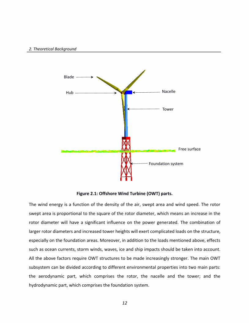
2.1 Offshore wind turbine (OWT) parts. . . . . . . . . . . . . . . . . . . . . . . . . . . . . . . . . . . 12
2.2 OWT foundations. A. Monopile B. Tripod C.Jacket . . . . . . . . . . . . . . . . . . . . . . . . 14
2.3 Pressure and velocity distribution over the actuator disk. . . . . . . . . . . . . . . . . . . . . . . 15
2.4 Flow vectors [65]. . . . . . . . . . . . . . . . . . . . . . . . . . . . . . . . . . . . . . . . . . . . . . 19
2.5 Single wave properties. . . . . . . . . . . . . . . . . . . . . . . . . . . . . . . . . . . . . . . . . . . 23
2.6 Shows an example of different wind shears for land and offshore area [24]. . . . . . . . . 27
3.1 Panel local coordinate system [54]. . . . . . . . . . . . . . . . . . . . . . . . . . . . . . . . . . . 34
3.2 Wake sheet behind an airfoil. . . . . . . . . . . . . . . . . . . . . . . . . . . . . . . . . . . . . . . . 36
3.3 Flowchart of blade-tower interaction procedure. . . . . . . . . . . . . . . . . . . . . . . . . . . 37
3.4 Color contour of pressure field around airfoil. . . . . . . . . . . . . . . . . . . . . . . . . . . . . . 42
4.1 2D airfoils types used in the design of the wind-turbine blades. . . . . . . . . . . . . . . . . . 47
4.2 3D OWT blade airfoils. . . . . . . . . . . . . . . . . . . . . . . . . . . . . . . . . . . . . . . . . . . . 47
4.3 Wind turbine geometry from different views. . . . . . . . . . . . . . . . . . . . . . . . . . . . . 49
4.4 Blade panels grid. . . . . . . . . . . . . . . . . . . . . . . . . . . . . . . . . . . . . . . . . . . . . . 50
4.5 Variation of the torque coefficient as a function of the number of grid points. . . . . . . . . . 51
4.6 Wake structure behind the wind turbine rotor. . . . . . . . . . . . . . . . . . . . . . . . . . . . 52
4.7 Wake split technique. . . . . . . . . . . . . . . . . . . . . . . . . . . . . . . . . . . . . . . . . . . . . 53
4.8 Domains dimensions. . . . . . . . . . . . . . . . . . . . . . . . . . . . . . . . . . . . . . . . . . . . . 54
4.9 Surface mesh on the blade. . . . . . . . . . . . . . . . . . . . . . . . . . . . . . . . . . . . . . . . . 55
4.10 Stationary and rotating domains volume mesh. . . . . . . . . . . . . . . . . . . . . . . . . . . . . 56
4.11 Boundary layers mesh at 𝑟/𝑅=0.65. . . . . . . . . . . . . . . . . . . . . . . . . . . . . . . . . . . . 57
4.12 𝑌𝑝𝑙𝑢𝑠 Values around the blade. . . . . . . . . . . . . . . . . . . . . . . . . . . . . . . . . . . . . . . 57
4.13 Blade pressure distribution on face side (pressure side). . . . . . . . . . . . . . . . . . . . . . . . 60
4.14 Blade pressure distribution on back side (suction side). . . . . . . . . . . . . . . . . . . . . . . . 60
4.15 Pressure coefficient distributions at different blade sections. . . . . . . . . . . . . . . . . . . . . . 62
4.16 Velocity contour over blade at different sections. . . . . . . . . . . . . . . . . . . . . . . . . . . . . 63
4.17 Pressure coefficient distributions shows blade–tower interaction using BEM. . . . . . . . . . . 65
List of Figures
viii
4.18 Pressure coefficient distributions shows blade–tower interaction using RANSE. . . . . . . . . . 65
4.19 Pressure distribution on the tower when the blade has 0o from tower
A. CFX B. panMARE C. On tower leading edge for both codes. . . . . . . . . . .
66
4.20 Pressure distribution on the tower when the blade has 60o from tower
A. CFX B. panMARE C. On tower leading edge for both codes. . . . . . . . . . . . 66
4.21 Time history of aerodynamic torque and thrust for case I and case II. . . . . . . . . . . . . . . . . 68
4.22 Time history of the tower force at inflow direction. . . . . . . . . . . . . . . . . . . . . . . . . . . 69
4.23 CFX setting for wave simulations. A. Domain B. Volume mesh at y=0. . . . . . . . . . . . . 71
4.24 CAD grid discretization. . . . . . . . . . . . . . . . . . . . . . . . . . . . . . . . . . . . . . . . . . . . 74
4.25 Split technique. . . . . . . . . . . . . . . . . . . . . . . . . . . . . . . . . . . . . . . . . . . . . . . . . 75
4.26 Geometries definitions. . . . . . . . . . . . . . . . . . . . . . . . . . . . . . . . . . . . . . . . . . . . 75
4.27 Flowchart procedure for calculating the hydrodynamic loads using Morison equation. . . . . 77 4.28 Time history for surface elevations (two meter from the cylinder). . . . . . . . . . . . . . . . . . . 80 4.29 Time history for wave velocity at inflow direction (two meter from the cylinder). . . . . . . . . . . 80
4.30 Time history for wave velocity at vertical direction (two meter from the cylinder). . . . . . . . . 81 4.31 Time history for wave dynamic pressure (two meter from the cylinder). . . . . . . . . . . . . . . 81
4.32 Time history for the inflow wave loads on the cylinder. . . . . . . . . . . . . . . . . . . . . . . 82 5.1 OWT with support structure. A. Monopile B. Tripod C. Jacket. . . . . . . . . . . . . . . . . . 86 5.2 Tripod support structure. . . . . . . . . . . . . . . . . . . . . . . . . . . . . . . . . . . . . . . . . . 87
5.3 Jacket support structure. . . . . . . . . . . . . . . . . . . . . . . . . . . . . . . . . . . . . . . . . . . 88
5.4 OWT modelling for BEM code. . . . . . . . . . . . . . . . . . . . . . . . . . . . . . . . . . . . . . . . . 89 5.5 Flowchart of BEM code procedure. . . . . . . . . . . . . . . . . . . . . . . . . . . . . . . . . . . . . . 90 5.6 Wind shear applying technique in BEM code. . . . . . . . . . . . . . . . . . . . . . . . . . . . . . 93 5.7 Wind velocity distribution according to log law. . . . . . . . . . . . . . . . . . . . . . . . . . . . . 93 5.8 Tripod foundation part. A. Panel grid B. Blocking strategy. . . . . . . . . . . . . . . . . 95 5.9 Jacket upper and lower parts. A. Panel grid B. Blocking strategy. . . . . . . . . . . . . . . 96 5.10 Jacket x- braces and k-joint. A. Panel grid B. Blocking strategy. . . . . . . . . . . . . . . 96 5.11 OWT panel grids. A. Monopile B. Tripod C. Jacket. . . . . . . . . . . . . . . . . . . . . . . . . 97 5.12 OWT models. A. Domain dimensions. B. Mesh domain. . . . . . . . . . . . . . . . . . . . . . . 100 5.13 Blade surface mesh and boundary layers. . . . . . . . . . . . . . . . . . . . . . . . . . . . . . . . . . 101 5.14 Log-law wind profile. . . . . . . . . . . . . . . . . . . . . . . . . . . . . . . . . . . . . . . . . . . . . 103 5.15 Wave kinematics. . . . . . . . . . . . . . . . . . . . . . . . . . . . . . . . . . . . . . . . . . . . . . . . 105 5.16 Pressure distribution on OWT with monopile foundation, water surface colored by the wave
elevation. . . . . . . . . . . . . . . . . . . . . . . . . . . . . . . . . . . . . . . . . . . . . . . . . . . 111
5.17 Pressure distribution on OWT with tripod foundation, water surface colored by the wave velocity at x-direction. . . . . . . . . . . . . . . . . . . . . . . . . . . . . . . . . . . . . . . . . . . .
112
5.18 Pressure distribution on OWT with jacket foundation, water surface colored by the wave velocity at z-direction. . . . . . . . . . . . . . . . . . . . . . . . . . . . . . . . . . . . . . . . . . . . . .
113
List of Figures
ix
5.19
Pressure distribution on monopile foundation. . . . . . . . . . . . . . . . . . . . . . . . . . . . .
114
5.20 Pressure distribution on tripod foundation. . . . . . . . . . . . . . . . . . . . . . . . . . . . . . . 115 5.21 Pressure distribution on jacket foundation. . . . . . . . . . . . . . . . . . . . . . . . . . . . . . . . 116 5.22 Time history of the thrust rotor contribution for OWT monopile case. . . . . . . . . . . . . . . 117 5.23 Time history of the thrust rotor contribution for OWT tripod case. . . . . . . . . . . . . . . . . . 117 5.24 Time history of the thrust rotor contribution for OWT Jacket case. . . . . . . . . . . . . . . . . . . 118 5.25 Time history for tower and monopile contribution. . . . . . . . . . . . . . . . . . . . . . . . . . . 118 5.26 Time history for tower and tripod contribution. . . . . . . . . . . . . . . . . . . . . . . . . . . . . 119 5.27 Time history for tower and jacket contribution. . . . . . . . . . . . . . . . . . . . . . . . . . . . . 119
5.28 Time history for the tower and monopile contribution for OWT monopile case. . . . . . . . . 120 5.29 Time history for the tower and tripod contribution for OWT tripod case. . . . . . . . . . . 120 5.30 Time history for the tower and jacket contribution for OWT jacket case. . . . . . . . . . . . 121 5.31 Total force on OWT with monopile foundation. . . . . . . . . . . . . . . . . . . . . . . . . . . . . . 121 5.32 Total force on OWT with tripod foundation. . . . . . . . . . . . . . . . . . . . . . . . . . . . . . . . 122 5.33 Total force on OWT with jacket foundation. . . . . . . . . . . . . . . . . . . . . . . . . . . . . . . . 122

List of Figures
x
xi
List of Tables
4.1 Wind turbine rotor geometry definition [7]. . . . . . . . . . . . . . . . . . . . . . . . . . . . 48
4.2 Boundary conditions for case I and case II. . . . . . . . . . . . . . . . . . . . . . . . . . . 57
4.3 Boundary conditions and general setting. . . . . . . . . . . . . . . . . . . . . . . . . . . . . 72
4.4 Wave kinematics at specified point. (2 m from cylinder leading edge). . . . . . . . . . 82
4.5 Loads at in flow direction on the cylinder using BEM and RANSE solvers besides Morison equation. . . . . . . . . . . . . . . . . . . . . . . . . . . . . . . . . . . . . . . . . . . . . . . . . . .
80
5.1 Panel grids number. . . . . . . . . . . . . . . . . . . . . . . . . . . . . . . . . . . . . . . . . . . 97
5.2 Waves properties . . . . . . . . . . . . . . . . . . . . . . . . . . . . . . . . . . . . . . . . . . . 98
5.3 Mesh generation setting. . . . . . . . . . . . . . . . . . . . . . . . . . . . . . . . . . . . . . . 99
5.4 OWT cases number of mesh. . . . . . . . . . . . . . . . . . . . . . . . . . . . . . . . . . . . . 101
5.5 Fluid specification. . . . . . . . . . . . . . . . . . . . . . . . . . . . . . . . . . . . . . . . . . . . . 102
5.6 Mean value for the last three amplitude loads on the OWT cases. . . . . . . . . . . . 108

List of Tables
xii

xiii
List of Symbols Roman Letters
Symbol Description Unit
𝐴 Area [𝑚2]
𝑎 Axial induction factor ----
𝑎∗ Angular induction factor ----
𝐵 Number of blades ----
𝑐 Airfoil chord [𝑚]
𝐶𝑝 Pressure coefficient ----
𝐶𝐷 Drag coefficient ----
𝐶𝐿 Lift coefficient ----
𝐶𝑀 Inertia coefficient ----
𝐶𝑄 Torque coefficient ----
𝑑 Water depth [𝑚]
𝐷 Drag force [𝑁]
𝐷𝑖 Diameter [𝑚]
𝐹 Force [𝑁]
𝑓𝐷 Wave drag force [𝑁]
𝑓𝐼 Wave inertia force [𝑁]
g Acceleration [𝑚2/s]
𝐻 Wave height [𝑚]
𝛪 Moment of inertia [kg 𝑚2]
𝑘 Wave number= 2𝜋 𝜆⁄ [𝑚−1]
KC keulegan-karpenter number ----
𝐿 Lift force [𝑁]
𝑚 Mass of a fluid inside a control volume [kg]
Mass flow rate [kg/s]
𝑛 Normal vector of a surface [𝑚,𝑚,𝑚]𝑇
𝑝 Pressure [𝑁 𝑚2⁄ ]
𝑃 Wind power [Watt]
𝑄 Torque [𝑁 𝑚]
List of Symbols
xiv
𝑅 Rotor radius [𝑚]
𝑟 Radius [𝑚]
𝑅𝑒 Reynolds number ----
𝑆 Surface area [𝑚2]
𝑆𝜁 Wave energy spectrum [𝑚2𝑠/𝑟𝑎𝑑]
𝑡 Time [𝑠]
T Thrust force [N]
𝑢, 𝑣, 𝑤 Velocity components [𝑚/𝑠]
𝑉 Volume [𝑚3]
𝑣 Air velocity [𝑚/𝑠]
X Distance [𝑚]
𝑥, 𝑦, 𝑧 Coordinate directions [𝑚]
Greek Letters Symbol Description Unit
α Angle of attack [ 𝜊]
𝛤 Circulation [𝑚2/𝑠]
𝜈 Kinematic viscosity [𝑚2/𝑠]
δ Volume fraction factor ----
𝜖 Exponent of the power law wind profile ----
𝜂 Wave displacement [𝑚]
𝜃 Pitch angle [ 𝜊]
𝜆 Wave length [𝑚]
𝜆𝑟 Tip speed ratio ----
μ Doublet strength [𝑚4 𝑠⁄ ]
𝜇0 Propagation direction of a seaway [ 𝜊]
𝜌 Fluid density [𝑘𝑔/𝑚3]
σ Source strength [𝑚3 𝑠⁄ ]
𝜗 Random value ----
𝛷∗ Total potential [𝑚2/𝑠]
𝛷∞ Potential of undisturbed flow [𝑚2/𝑠]
𝜓 Mean wave direction [ 𝜊]
𝜔 Angular frequency [1/𝑠]
𝛺 Rotor angular velocity [𝑟𝑎𝑑/𝑠]

List of Symbols
xv
Sub- and Superscripts 𝑐. 𝑣 Control volume
𝑐. 𝑠. Control surface
𝑖𝑛 Inlet
𝑖𝑛𝑑 Induced
𝑅 Rotor
𝑆𝑤 Wake surface
𝑆𝐵 Surface boundary
𝑡. 𝑒 Trailing edge
𝑤 Wake far field
∞ Free stream
+ - Values around actuator disc Average value
Abbreviations BEM Boundary Element Method
CFD Computational Fluid Dynamics
HAWT Horizontal-axis wind turbine
𝑁𝑂𝑃 Number of Panel
NREL National Renewable Energy Laboratory
OWT Offshore Wind Turbine
RANSE Reynolds-Averaged Navier-Stokes Equation
VOF Volume of Fluid

List of Symbols
xvi
1
Introduction
While wind power, as an important source of renewable energy, has primarily been utilized on
land, generating electricity using offshore wind turbines (OWTs) is becoming increasingly
important. Utilizing wind land is not a new technology, as the first attempts to extract electrical
energy from wind began in the 19th century [50]. Wind land energy will remain dominant in the
near future, but wind energy at sea regions will become a more efficient technology. Although
the first concept for large-scale OWTs was introduced by William E. Heronemus at the University
of Massachusetts Amherst as early as 1972, it was not implemented until 1990.
Due to the higher speed of offshore wind, offshore wind energy is being given priority over land
wind. Given the fact that the power content of wind increases with the cube of the wind velocity,
offshore wind is able to deliver more power than land wind [80]. Further, due to its high humidity,
wind or air in sea regions has more density than in land areas: the kinetic energy of the air is a
function of its density, of its mass per volume unit. Thus, the high density of the air vapor mixture
means that OWTs are able to convert more energy.
Offshore wind is generally less turbulent than on land, meaning that it is relatively easier to
efficiently operate an OWT. When taking into consideration that no obstacles are present except
islands, the turbulence of the sea surface layer will be lower than on land because temperature
differences at different altitudes of the atmosphere are lower. This means that wind speed does
not suffer major changes and the kinds of high towers necessary for land turbines are no longer
needed, which further leads to lower mechanical fatigue load and thus a longer lifetime for
turbines, reducing material and maintenance costs [26].

1. Introduction
2
Offshore wind energy can help to decrease greenhouse gas emissions, increase the diversity of
energy supply sources, provide cost‐competitive electricity to coastal regions, all of which can
have positive economic benefits [92]. The OWT-supporting structure is a relatively complex
geometry that can withstand severe loads and be subjected to multiple environmental conditions
as result of high wave amplitudes, currents, and wind velocities. OWT design can be carried out
regarding different objectives, such as high efficiency, light structure, and adequate fatigue life
[13]. Achieving such goals requires accurate consideration of all environmental conditions around
the OWT location.
Other issues must also be taken into account, such as corrosion and special protection of the
electric and mechanical components of the wind turbine from high humidity, the transportation
of huge structures from the production location on land to harbours, and other technical
challenges such as installation and grid interconnection.
1.1 Numerical Background
1.1.1 Aerodynamic Methods Review
There are several methods of varying levels of complexity that can be used to predict the
aerodynamic loads on OWT aerodynamic parts. Blade element momentum method has been
very popular for OWT design and analysis [38]. A number of comprehensive computer codes are
based on this method such as [71]. This method is highly efficient and cheap but it incapable of
accurately modelling three-dimensional cross flow, tower shadow effects and tip losses, which
are considered by employing empirical corrections. Researchers have attempted to increase the
accuracy of this method [82, 14] by developing various tip loss corrections.
1. Introduction
3
In order to model the OWT aerodynamics with higher computational efficiency, potential flow
models have been introduced, including lifting line, panel, and vortex lattice methods. Generally,
in these models, the blade is modeled by lifting line, lifting surface or lifting panels and the wake
can be modelled by either trailing vortices or vortex ring elements. These methods can be used
for more complex flows, including tower shadow effects and non-axial inflow condition. But it
cannot predict stall phenomena because the viscous effects are still not taken into consideration.
The accuracy of the solution in all of these methods is quite acceptable, Abedi et al. [2] used a
vortex based method for modelling wind turbine aerodynamic performance and compared it with
three different approaches of lifting line, lifting surface, and panel method models. Results proved
the higher capability of the panel method to calculate detailed load as well as the pressure and
velocity distributions over the blade surface compared to other approaches.
Gephardt et al. [31] has utilized a vortex-lattice method to simulate the unsteady aerodynamic
behavior of large horizontal-axis wind turbines in time domain. The aerodynamic blade-tower
interaction has been satisfactorily captured as well as the effects of land surface and boundary
layer. Kim et al. [52] have used the unsteady vortex-lattice method to simulate the blade-tower
interaction over the NREL Phase VI. Further, they used the nonlinear vortex correction method to
investigate the rotor turbine while considering wind shear, yaw error, distance from blade to
tower, and the size of the tower. A three-dimensional panel method was used by Bermudez et al.
[11] for simulating the aerodynamic behavior of horizontal-axis wind turbines, and the
comparison between experimental data and the computed results with the panel method shows
a good agreement. The lifting lines model used by Dumitresch et al. [19] to simulate horizontal-
axis wind turbines (HAWTs) delivered better results by using a nonlinear iterative prescribed
wake analysis in comparison with the free wake model.
1. Introduction
4
The results of different research groups show that potential flow-based methods are very efficient
for calculating the aerodynamic loads on horizontal-axis wind turbine blades. Employing a higher
level of complexity, as an example, the RANSE solver in combination with an appropriate
turbulence model allows for a more accurate flow simulation but also increases the
computational time. Lee et al. [57] used a RANSE solver in combination with the Spalart-Allmaras
turbulence model to evaluate the performance of a blade with blunt airfoil which was adapted at
the blade’s root by increasing the blunt trailing-edge thickness to 1%, 5% and 10% of the chord.
The blunt trailing-edge blade helps to improve the structure performance of the blades.
Derakhshan et al. [22] compared the Spalart-Allmaras, k-ε and SST k-ω turbulence models for
estimating aerodynamic performance of wind turbine blades. The results show that at low wind
speeds, all three turbulence models have similar predictions in power, but at higher wind speeds,
the results predicted by the k-ε model are more accurate.
Further, the SST turbulence model [67] is widely used for wind turbine simulations due to its
ability to simulate attached and lightly separated airfoil flows. This model is also used in Keerthana
et al. [51] to obtain the aerodynamic analysis of 3 kW small HAWT. The large eddy simulation
model, which is more complicated, has the ability to more accurately resolve flow separation and
the stall of an airfoil [40]. However, the simulation computational time is significantly higher than
any of the methods previously mentioned. Several authors have performed CFD computations of
different OWT geometries for a variety of aims. Zhao et al. [110] has investigated the
aerodynamics of the NREL 5MW offshore HAWT, including the blade-tower interaction and the
rotor wake development downstream by utilizing the RANSE solver U2NCLE. The computational
analysis provides insight into the aerodynamic performance of the upwind and downwind, two-
and three-bladed HAWTS. Moshfeghi et al. [68] has investigated the effects of near-wall grid
spacing and has studied the aerodynamic behavior of a NREL Phase VI HAWT by comparing thrust
forces, flow patterns and pressure coefficients at different wind speeds.
1. Introduction
5
Elfarra [25] has studied rotor optimization using CFD to calculate the optimized winglet, twist
angle distribution and pitch angle for a wind turbine blade. Choi et al. [16] has presented the
results on power production due to wake effects stemming from the distance between two wind
turbines in a wind farm. Hsu et al. [33] have used a RANS-code, which based on the finite element-
based Arbitrary-Lagrange-Eulerian method formulation to simulate the NREL Phase VI wind
turbine in a wide range of wind velocities with a rotor configuration only, and the full wind turbine
with the sliding interface method. Bazilevs et al. [7] have carried out CFD simulations on the flow
over the NREL 5MW offshore wind turbine rotor using both a finite element approach and a
NURB-based (Non-Uniform Rational B-splines) approach for the geometry and have
demonstrated the capability of the method to perform a coupled aerodynamic structural analysis.
They also used the same approach in [8] to simulate the three-blade 5MW wind turbine for
flexible and rigid blades, with and without the presence of the tower. In order to incorporate the
effect of the wind turbine tower into the simulations, the rotationally-periodic boundary
conditions were excluded, and as a result, the blade-tower interaction was successfully
investigated.
1.1.2 Hydrodynamic Methods Review
In this section, a review of methods used to calculate the hydrodynamic load on different
foundation types (support structure) using different wave formulations are presented.
Morison Equation [66] is widely applied to calculate the hydrodynamic loads on the slender
structure where the diffraction is adopted. MacCamy et al. [61] used linear diffraction theory for
computing wave forces on cylindrical offshore structures. Linear part of the Morison equation
and linear diffraction theory can be combined for calculating the wave force on a structure in case
1. Introduction
6
that the ratio between the diameter of the structure and the wave length as well as the wave
amplitude does not exceed certain limits, see Chakrabarti et al. [17].
Manners [62] has used potential flow to calculate the fluid load on a circular cylinder. The results
were used to compare the calculated inertia force component of the wave load on the cylindrical
members of offshore structures with the value estimated by the conventional Morison equation
formulation. A numerical model based on a panel method was used by Haas [34] to simulate the
influence of water waves on constructions.
To improve the accuracy of the calculation of the hydrodynamic force, Seok et al. [83] have used
the RANSE solver to evaluate the wave and current loads on a fixed cylindrical platform model for
an offshore wind turbine. They compared the results with the corresponding values obtained by
the Morison formula and the experimental data, where the CFD results show a reasonable
agreement with the experimental data and the Morison formula results only for the case that
progressive wave is considered. However, when current is included, CFD predicts smaller loads
than the Morison formula. Similarly, Damgaard et al. [20] compared the results obtained by the
Morison equation with the RANSE solver. The comparisons were made for regular, irregular, and
breaking waves. Markus et al. [63] utilized a RANSE solver with the combination of a non-linear
wave model with a volume of fluid calculation to generate an unsteady sea state. A simulation
strategy that focuses on capturing wave-current interaction is introduced and is validated with
respect to fluid particle kinematics.
In another approach, Li [106] focused on the dynamic structure response for a 70 m jacket using
a finite element method. The results of the hydrodynamic analysis allow the comparison of wave
loads with different regular wave theories, including: extrapolated Airy theory, stretched wave
theory, the 5th-order Stokes wave theory and stream function theory. Further, the multi-physics
finite-
1. Introduction
7
element based nonlinear numerical code LS-DYNA, containing both fluid and structural models,
was carried out by Zhang [107].
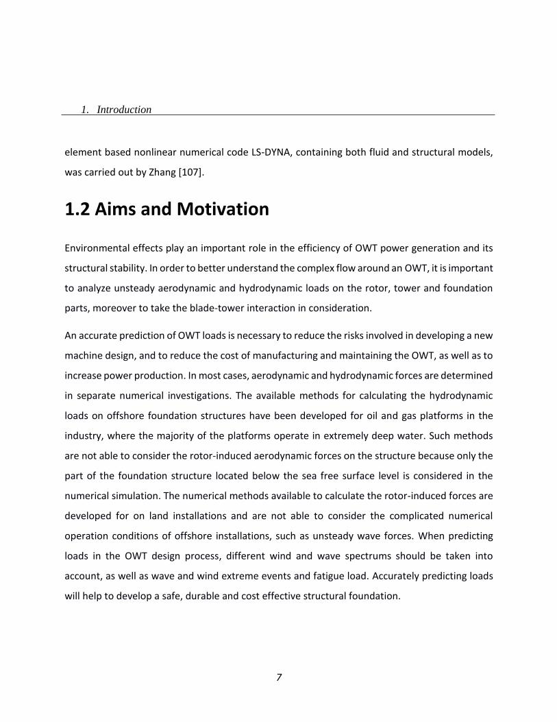
1.2 Aims and Motivation
Environmental effects play an important role in the efficiency of OWT power generation and its
structural stability. In order to better understand the complex flow around an OWT, it is important
to analyze unsteady aerodynamic and hydrodynamic loads on the rotor, tower and foundation
parts, moreover to take the blade-tower interaction in consideration.
An accurate prediction of OWT loads is necessary to reduce the risks involved in developing a new
machine design, and to reduce the cost of manufacturing and maintaining the OWT, as well as to
increase power production. In most cases, aerodynamic and hydrodynamic forces are determined
in separate numerical investigations. The available methods for calculating the hydrodynamic
loads on offshore foundation structures have been developed for oil and gas platforms in the
industry, where the majority of the platforms operate in extremely deep water. Such methods
are not able to consider the rotor-induced aerodynamic forces on the structure because only the
part of the foundation structure located below the sea free surface level is considered in the
numerical simulation. The numerical methods available to calculate the rotor-induced forces are
developed for on land installations and are not able to consider the complicated numerical
operation conditions of offshore installations, such as unsteady wave forces. When predicting
loads in the OWT design process, different wind and wave spectrums should be taken into
account, as well as wave and wind extreme events and fatigue load. Accurately predicting loads
will help to develop a safe, durable and cost effective structural foundation.
1. Introduction
8
The aim of this research is the further development of the in-house boundary element method
code – panMARE – in order to simulate the unsteady flow behavior of a full offshore wind turbine
in combination with aerodynamic and hydrodynamic loads in time domain.
The results obtained using the BEM code are compared with the results obtained from RANSE
solver calculations, which are carried out by using ANSYS CFX. These comparisons will highlight
the viscous effects of the OWT system which are not considered in the BEM code and will point
to the limitations and possibilities of the inviscid flow model to predict the complex OWT loading.
The inviscid flow model is applied for simulating ship propellers and returns reliable results, as in
[32] [9]. Different techniques for the BEM code are developed within this work in order to
simulate OWT. The first regards solving the blade-tower interaction problem. In this case, a
special treatment must be applied for the wake panels that collide with the tower. And the second
technique is the further development of the BEM code to be able to estimate both aerodynamic
and hydrodynamic loads, which is achieved by combining two solvers in one iteration.
The structure of this thesis is organized as follows. In Chapter 2, the first subsection describes a
general OWT parts-configuration model. The second subsection is devoted to explaining the basic
aerodynamic and hydrodynamic concepts, followed by a discussion of the OWT. The chapter is
finalized by a description of the wind shear flow over offshore region. In Chapter 3, the initial
subsections are dedicated to providing details about the BEM code, including the governing
equations, boundary conditions, blade-tower interaction and wave generation part. The second
subsection for this chapter describes the applied viscous flow solver, including the governing
equation, the turbulence flow model and the VOF technique, which is used to track the free
surface. In Chapter 4, three test model simulations are presented, which are conducted using
BEM and RANSE methods, for three different configurations (OWT rotor, land wind turbine and
monopile). There are two main parts in this chapter: OWT aerodynamic simulations and OWT
hydrodynamic simulations.
1. Introduction
9
In the first subsection, OWT rotor and land wind turbine are analyzed using both applied methods.
This subsection presents some details of the investigated geometry, the mesh generation and the
general solvers setting for both solvers. The validation and comprehensive comparison between
the results of the two applied methods are also presented. In the second subsection, OWT
hydrodynamic simulations include the calculation of the flow around the slender cylinder under
the effect of 2D sea waves. This subsection starts with the model description followed by the
solution setting for both solvers and concludes with a discussion of the results. For validating this
test case, the calculated cylinder forces achieved via the different method are compared with the
values obtained by the Morison equation.
In Chapter 5, the full OWT is analyzed via both the BEM and RANS methods, with the combination
of wind and free surface water waves effects. The 5MW NREL rotor model is used as the baseline
model in the simulation studies with three different foundations types, including monopile, tripod
and jacket. The chapter begins with a general description of the configurations used for the
modelling, followed by some details about the fully coupled wind and wave loads, and the solver
required setting for the BEM method. The second part of this chapter describes the simulation of
the viscous flow on OWT using RANSE solver, followed by a comparison of the calculated results.

1. Introduction
10

11
Theoretical Background
The purpose of this chapter is to give an overview on the relevant physics that describe the flow
around the OWT and to explain the most important aspects of the OWT aero- and hydro dynamics
resulting from wind and wave effects. The first part of this chapter describes the main OWT
components. The following section then discusses the basic aerodynamic concepts. Thereafter,
hydrodynamic models and wave properties are presented. This is followed by the overall
aerodynamic and hydrodynamic OWT loading. The chapter ends with a discussion on wind shear
over offshore regions. A good understanding of the physics of the flow will help to elucidate the
mathematical model choices in the next chapter.
2.1 Offshore Wind Turbine (OWT)
An offshore wind turbine (OWT) is a device that extracts kinetic energy from offshore wind and
converts it into mechanical energy. OWT systems basically consist of a rotor, a tower, a nacelle,
and foundation system, as shown in Figure 2.1. OWTs can produce large quantities of electricity
as compared to other energy sources. The torque generated in the rotor due to the passing wind
will push the blades with determined forces that convert the wind kinetic energy into a certain
amount of mechanical energy in the generator (stator).
2. Theoretical Background
12
Figure 2.1: Offshore Wind Turbine (OWT) parts.
The wind energy is a function of the density of the air, swept area and wind speed. The rotor
swept area is proportional to the square of the rotor diameter, which means an increase in the
rotor diameter will have a significant influence on the power generated. The combination of
larger rotor diameters and increased tower heights will exert complicated loads on the structure,
especially on the foundation areas. Moreover, in addition to the loads mentioned above, effects
such as ocean currents, storm winds, waves, ice and ship impacts should be taken into account.
All the above factors require OWT structures to be made increasingly stronger. The main OWT
subsystem can be divided according to different environmental properties into two main parts:
the aerodynamic part, which comprises the rotor, the nacelle and the tower; and the
hydrodynamic part, which comprises the foundation system.
Tower
Nacelle
s Hub
Blade
Free surface
Foundation system

2. Theoretical Background
13
2.1.1 Rotor, Nacelle and Tower
The rotor is made of a certain number of blades (normally three) and a hub. The blade design is
similar to that used in airplane technology. Force is generated due to different pressures between
the lower side and the upper side of the blade. Both the shape of the blade airfoils and its angle
relative to wind direction will affect its aerodynamic performance. The rotor is subjected to
different environmental conditions such as changing wind speeds and wind directions, where the
wind velocity at the tip of the rotor blade is higher than at the center of the hub. The nacelle,
which connects the hub to the tower, houses the main components of the OWT, such as the
controller, gearbox, generator and shafts, and serves to protect these sensitive parts from
environmental factors.
The tower supports the OWT nacelle and rotor and elevates the rotor to a height at which the
wind velocity is higher and less turbulent than at sea level, due to the wind shear effect. The
tower’s structure must be able to resist the severe loads originating from gravitational, rotational
and wind thrust forces.
2.1.2 Foundation System
The foundation serves as a support to all upper OWT structures. It extends from the seabed level
to above water level and connects to the tower via a transition piece. Different types of
foundations can be used for the installation of offshore wind turbines.
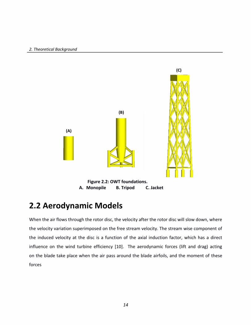
For water depths up to (40 m), monopile or tripod structures can be used. Jacket foundations are
the most economical choice for water depths of more than 40m. For even larger water depths
(100-300m), floating wind turbines might be the only economical choice. In the present study,
three types of fixed foundations are investigated: monopile, tripod and jacket, all of which are
shown in Figure 2.2.
2. Theoretical Background
14
2.2 Aerodynamic Models
When the air flows through the rotor disc, the velocity after the rotor disc will slow down, where
the velocity variation superimposed on the free stream velocity. The stream wise component of
the induced velocity at the disc is a function of the axial induction factor, which has a direct
influence on the wind turbine efficiency [10]. The aerodynamic forces (lift and drag) acting
on the blade take place when the air pass around the blade airfoils, and the moment of these
forces
Figure 2.2: OWT foundations. A. Monopile B. Tripod C. Jacket
(A)
(B)
(C)
2. Theoretical Background
15
𝒑𝒓𝒐𝒕𝒐𝒓−
𝒑∞
Actuator disk (rotor)
𝒗∞ 𝒗𝒓𝒐𝒕𝒐𝒓
Velocity
𝒗𝒘
𝒑∞ Pressure
𝒑𝒓𝒐𝒕𝒐𝒓+
deliver the required torque to generate the output power. The torque and power values can be
calculated depending on a flow around the rotor. Different theories can be applied to estimate
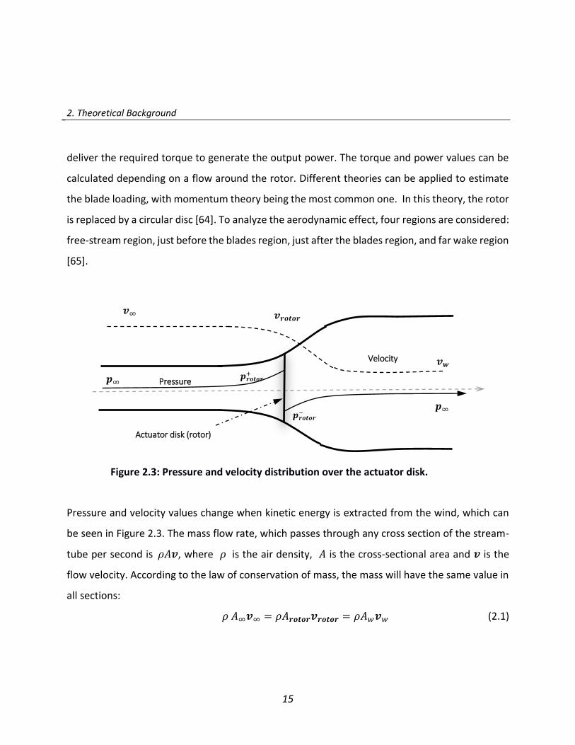
the blade loading, with momentum theory being the most common one. In this theory, the rotor
is replaced by a circular disc [64]. To analyze the aerodynamic effect, four regions are considered:
free-stream region, just before the blades region, just after the blades region, and far wake region
[65].
Pressure and velocity values change when kinetic energy is extracted from the wind, which can
be seen in Figure 2.3. The mass flow rate, which passes through any cross section of the stream-
tube per second is 𝜌𝐴𝒗, where 𝜌 is the air density, 𝐴 is the cross-sectional area and 𝒗 is the
flow velocity. According to the law of conservation of mass, the mass will have the same value in
all sections:
𝜌 𝐴∞𝒗∞ = 𝜌𝐴𝒓𝒐𝒕𝒐𝒓𝒗𝒓𝒐𝒕𝒐𝒓 = 𝜌𝐴𝑤𝒗𝑤 (2.1)
Figure 2.3: Pressure and velocity distribution over the actuator disk.

2. Theoretical Background
16
The fraction by which the axial component of velocity is reduced, is the axial induction factor (𝑎).
If the free stream velocity is 𝒗∞ and the axial velocity at the rotor plane is 𝒗𝒓𝒐𝒕𝒐𝒓, then the axial
induction factor is:
𝑎 =𝒗∞−𝒗𝑟𝑜𝑡𝑜𝑟
𝒗∞ (2.2)
The overall change in velocity when air passes through the disc can be defined as 𝒗∞ − 𝒗𝑤 , and
a rate of axial momentum change equal to the overall change of velocity times the mass flow rate
is:
𝑅𝑎𝑡𝑒 𝑜𝑓 𝑐ℎ𝑎𝑛𝑔𝑒 𝑜𝑓 𝑚𝑜𝑚𝑒𝑛𝑡𝑢𝑚 = (𝒗∞ − 𝒗𝑤)𝜌𝐴𝒓𝒐𝒕𝒐𝒓𝒗𝒓𝒐𝒕𝒐𝒓 (2.3)
The force causing this change of momentum comes from the pressure difference across the disc
area. (𝑝𝒓𝒐𝒕𝒐𝒓+ − 𝑝𝒓𝒐𝒕𝒐𝒓
− )𝐴𝒓𝒐𝒕𝒐𝒓 = ( 𝒗∞ − 𝒗𝑤)𝜌𝐴𝒓𝒐𝒕𝒐𝒓𝒗𝒓𝒐𝒕𝒐𝒓 (2.4)
The Bernoulli equation is applied separately for upstream regions and downstream regions to
obtain the pressure difference(𝑝𝒓𝒐𝒕𝒐𝒓+ − 𝑝𝒓𝒐𝒕𝒐𝒓
− ):
(𝑝𝒓𝒐𝒕𝒐𝒓+ − 𝑝𝒓𝒐𝒕𝒐𝒓
− ) = 0.5𝜌(𝒗∞2 − 𝒗𝑤
2 ) (2.5)
Separate equations are necessary because the total energy is different upstream and downstream
regions. Bernoulli's equation provides that, under steady conditions, the total energy in the flow,
comprising of kinetic energy, static pressure energy and gravitational potential energy, remains
constant provided no work is done on or by the fluid upstream.
The velocity component of the induced flow at the disc can be obtained by combining Eqs. (2.4)
and (2.5) and to furthermore define it with respect to the axial induction factor (𝑎) from Eq. (2.2):
𝒗𝒓𝒐𝒕𝒐𝒓 =𝒗∞+𝒗𝒘
𝟐 (2.6)
𝒗𝒓𝒐𝒕𝒐𝒓 = 𝒗∞(1 − 𝑎)

2. Theoretical Background
17
The velocity at far wake region can be defined as:
𝒗𝒘 = 𝒗∞(1 − 2𝑎) (2.7)
So the force equation (thrust) is then:
𝑇 = (𝑝𝒓𝒐𝒕𝒐𝒓+ − 𝑝𝒓𝒐𝒕𝒐𝒓
− )𝐴𝒓𝒐𝒕𝒐𝒓 = 2𝜌𝐴𝒓𝒐𝒕𝒐𝒓 𝒗∞2 𝑎(1 − 𝑎) (2.8)
Thrust coefficient 𝐶𝑇 is defined as: 𝐶𝑇 =𝑇
0.5𝜌𝒗∞2 𝐴𝒓𝒐𝒕𝒐𝒓
= 4𝑎(1 − 𝑎) (2.9)
The power in the approaching wind that is extracted at the rotor plane is defined as the rate of
work done by this force:
𝑃𝑜𝑤𝑒𝑟 = 𝐹𝑣𝒓𝒐𝒕𝒐𝒓 = 2𝜌𝐴𝒓𝒐𝒕𝒐𝒓 𝒗∞3 𝑎(1 − 𝑎)2 (2.10)
The power coefficient can be calculated with respect to available a power as:
𝐶𝑝𝑜𝑤𝑒𝑟 =𝑃𝑜𝑤𝑒𝑟
0.5𝜌𝒗∞3 𝐴𝒓𝒐𝒕𝒐𝒓
= 4𝑎(1 − 𝑎)2 (2.11)
The rotor can produce the maximum power when 𝐶𝑝𝑜𝑤𝑒𝑟 = 16/27 and 𝐶𝑇 = 8/9 for a = 1/3,
which is known as the Betz limit [65].
The stream tube introduced in Figure 2.3 can be discretized into annular elements of width 𝑑𝑟
and 𝑑𝐴 = 2𝜋𝑟𝑑𝑟. The momentum at axial direction can be applied to find the thrust on this
control volume using Eq. (2.8)
𝑑𝑇 = 2𝜌𝑟𝜋 𝒗∞2 𝑎(1 − 𝑎)𝑑𝑟 (2.12)
At the wake region, the induced velocity of the air will rotate in the opposite direction relative to
the blades. The blade wake rotates with an angular velocity ω𝑤and the blades rotate with an
angular velocity of Ω. As in axial direction, there must be a balance of angular momentum as well:
Angular moment = 𝛪𝜔𝑤 (2.13)
2. Theoretical Background
18
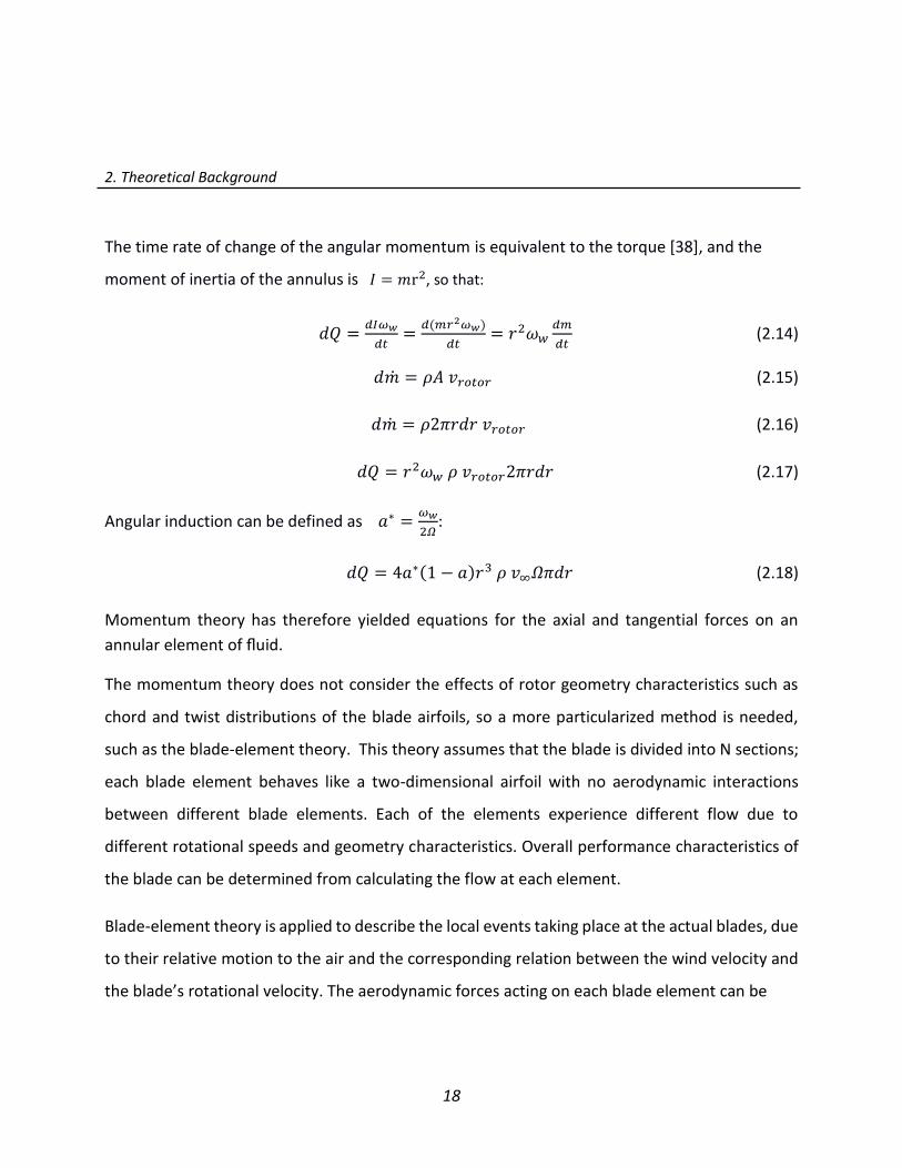
The time rate of change of the angular momentum is equivalent to the torque [38], and the
moment of inertia of the annulus is 𝛪 = 𝑚r2, so that:
𝑑𝑄 =𝑑𝛪𝜔𝑤
𝑑𝑡=𝑑(𝑚𝑟2𝜔𝑤)
𝑑𝑡= 𝑟2𝜔𝑤
𝑑𝑚
𝑑𝑡 (2.14)
𝑑 = 𝜌𝐴 𝑣𝑟𝑜𝑡𝑜𝑟 (2.15)
𝑑 = 𝜌2𝜋𝑟𝑑𝑟 𝑣𝑟𝑜𝑡𝑜𝑟 (2.16)
𝑑𝑄 = 𝑟2𝜔𝑤 𝜌 𝑣𝑟𝑜𝑡𝑜𝑟2𝜋𝑟𝑑𝑟 (2.17)
Angular induction can be defined as 𝑎∗ =𝜔𝑤
2𝛺:
𝑑𝑄 = 4𝑎∗(1 − 𝑎)𝑟3 𝜌 𝑣∞𝛺𝜋𝑑𝑟 (2.18)
Momentum theory has therefore yielded equations for the axial and tangential forces on an
annular element of fluid.
The momentum theory does not consider the effects of rotor geometry characteristics such as
chord and twist distributions of the blade airfoils, so a more particularized method is needed,
such as the blade-element theory. This theory assumes that the blade is divided into N sections;
each blade element behaves like a two-dimensional airfoil with no aerodynamic interactions
between different blade elements. Each of the elements experience different flow due to
different rotational speeds and geometry characteristics. Overall performance characteristics of
the blade can be determined from calculating the flow at each element.
Blade-element theory is applied to describe the local events taking place at the actual blades, due
to their relative motion to the air and the corresponding relation between the wind velocity and
the blade’s rotational velocity. The aerodynamic forces acting on each blade element can be
2. Theoretical Background
19
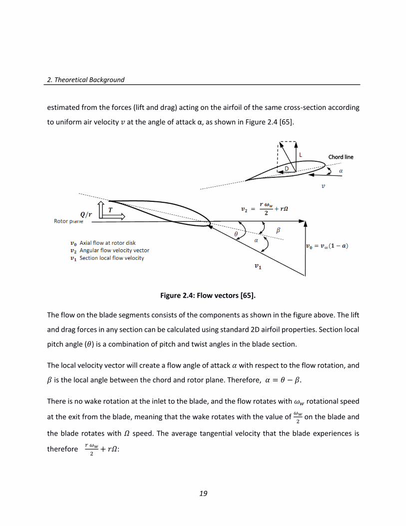
estimated from the forces (lift and drag) acting on the airfoil of the same cross-section according
to uniform air velocity 𝑣 at the angle of attack α, as shown in Figure 2.4 [65].
The flow on the blade segments consists of the components as shown in the figure above. The lift
and drag forces in any section can be calculated using standard 2D airfoil properties. Section local
pitch angle (𝜃) is a combination of pitch and twist angles in the blade section.
The local velocity vector will create a flow angle of attack 𝛼 with respect to the flow rotation, and
𝛽 is the local angle between the chord and rotor plane. Therefore, 𝛼 = 𝜃 − 𝛽.
There is no wake rotation at the inlet to the blade, and the flow rotates with 𝜔𝑤 rotational speed
at the exit from the blade, meaning that the wake rotates with the value of 𝜔𝑤
2 on the blade and
the blade rotates with 𝛺 speed. The average tangential velocity that the blade experiences is
therefore 𝑟 𝜔𝑤
2+ 𝑟𝛺:
Figure 2.4: Flow vectors [65].
2. Theoretical Background
20
𝑟 𝜔𝑤2
+ 𝑟𝛺 = 𝑟𝛺(1 + 𝑎∗) (2.19)
𝑡𝑎𝑛 𝜃 = 𝑣∞(1 − 𝑎)
𝑟𝛺(1 + 𝑎∗) (2.20)
𝑣1 sin 𝜃 = 𝑣∞(1 − 𝑎) (2. 21)
𝑣1 cos 𝜃 = 𝑟𝛺(1 + 𝑎∗) (2.22)
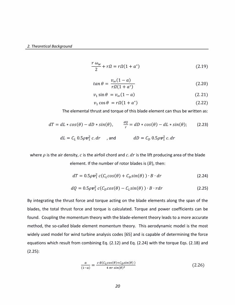
The elemental thrust and torque of this blade element can thus be written as:
𝑑𝑇 = 𝑑𝐿 ∗ 𝑐𝑜𝑠(𝜃) − 𝑑𝐷 ∗ 𝑠𝑖𝑛(𝜃), 𝑑𝑄
𝑟= 𝑑𝐷 ∗ 𝑐𝑜𝑠(𝜃) − 𝑑𝐿 ∗ 𝑠𝑖𝑛(𝜃); (2.23)
𝑑𝐿 = 𝐶𝐿 0.5𝜌𝒗12 𝑐. 𝑑𝑟 , and 𝑑𝐷 = 𝐶𝐷 0.5𝜌𝒗1
2 𝑐. 𝑑𝑟
where 𝜌 is the air density, 𝑐 is the airfoil chord and 𝑐. 𝑑𝑟 is the lift producing area of the blade
element. If the number of rotor blades is (𝐵), then:
𝑑𝑇 = 0.5𝜌𝒗12 𝑐(𝐶𝐿𝑐𝑜𝑠(𝜃) + 𝐶𝐷𝑠𝑖𝑛(𝜃) ) ∙ 𝐵 ∙ 𝑑𝑟 (2.24)
𝑑𝑄 = 0.5𝜌𝒗12 𝑐(𝐶𝐷𝑐𝑜𝑠(𝜃) − 𝐶𝐿𝑠𝑖𝑛(𝜃) ) ∙ 𝐵 ∙ 𝑟𝑑𝑟 (2.25)
By integrating the thrust force and torque acting on the blade elements along the span of the
blades, the total thrust force and torque is calculated. Torque and power coefficients can be
found. Coupling the momentum theory with the blade-element theory leads to a more accurate
method, the so-called blade element momentum theory. This aerodynamic model is the most
widely used model for wind turbine analysis codes [65] and is capable of determining the force
equations which result from combining Eq. (2.12) and Eq. (2.24) with the torque Eqs. (2.18) and
(2.25):
𝑎
(1−𝑎)= 𝑐∙𝐵(𝐶𝐿𝑐𝑜𝑠(𝜃)+𝐶𝐷𝑠𝑖𝑛(𝜃) )
4 𝜋𝑟 𝑠𝑖𝑛(𝜃)2 (2.26)

2. Theoretical Background
21
𝑎∗
(1 − 𝑎)= 𝑐 ∙ 𝐵(𝐶𝐷𝑐𝑜𝑠(𝜃) − 𝐶𝐿𝑠𝑖𝑛(𝜃) )
8 𝜋𝑟 𝑠𝑖𝑛(𝜃)2𝜆𝑟 (2.27)
Where 𝜆𝑟 is the local tip speed ratio 𝜆𝑟 =𝑟𝛺
𝑣∞ . So far, all necessary equations for this method
have been derived and the algorithm can be summarized by initializing 𝑎 and 𝑎∗= 0 and by
calculating the flow angle in Eq. (2.20) and the angle of attack, 𝐶𝐿 and 𝐶𝐷 values can be found.
𝑎 and 𝑎∗can be calculated from Eq. (2.26) and Eq. (2.27), and iteration continues until the value
of 𝑎 and 𝑎∗converge (error less than 1%), after which the axial force and torque can be calculated
as in Eq. (2.12) and Eq. (2.18). Although the BEM theory has the ability to calculate very quickly,
good experimental airfoil data and several empirical correction factors are necessary. Lifting line,
panel and vortex methods are aerodynamic models which have been developed based on
potential theory in order to obtain more detailed descriptions of the 3D flow around a wind
turbine and other applications. The potential flow theory assumes the fluid is inviscid,
incompressible and irrotational. Despite the fact that viscous effects are neglected, it is widely
used to predict the performance of different turbomachinery cases [11, 31, and 35]. The rotor
blades and the shed vortices in the wake can be represented by lifting lines or surfaces. The bound
circulation is generated from the aerodynamic forces when the flow passes the blades, so the
vortex strength on the blades depends on the blade circulation distribution. The wake panels are
generated due to the variation of the bound circulation at the panel trailing edge. The induced
velocity 𝒗𝑖𝑛𝑑 can be found at any point using the Biot-Savart induction law:
𝒗𝑖𝑛𝑑 = −1
4𝜋∫(𝑥 − 𝑥′) ∗ 𝜔′
|𝑥 − 𝑥′|3𝑑𝑉 (2.28)
𝜔′ is the vorticity, 𝑥 -𝑥′ is the distance between the integration point and the considered point.

2. Theoretical Background
22
The lifting force value can be calculated by applying the Kutta-Joukowski theorem. A simple
relationship between the bound circulation and the lift coefficient can be derived as:
𝐿 = 𝜌𝑣Γ = 0.5𝜌𝑣2 𝑐 𝐶𝐿 , Γ = 0.5𝜌𝑣 𝑐 𝐶𝐿 (2.29)
The wake form for this model can be prescribed as a hub vortex plus a spiraling tip vortex, or as a
series of ring vortices. Another aerodynamics model approach is panel method, which applies a
surface distribution of sources and doublets. The panel method is developed from Green’s
theorem, which allows for obtaining an integral representation of any potential flow field in terms
of singularity distribution. More details on this can be found in the next chapter.
2.3 Hydrodynamic Models
Determining the wave particle kinematics is essential for calculating the hydrodynamic loading
on a submerged structure in the time domain. Sea waves are random, short crested and have
various lengths in nature. Surface waves can be seen traveling in every direction. The wave can
be described as a wave spectrum and the calculations can begin by converting the spectrum back
into individual sinusoidal waves, as in Figure 2.5. The wave form and its specific effects depend
on several factors such as water depth, the distance the wave travels over the sea before reaching
the site and significant wave heights [44]. Further, the shape of the seabed will affect the wave’s
steepness.
The sinusoid waves particle velocity and acceleration vectors and dynamic pressure can be
calculated using linear Airy wave theory, which represents the first-order approximation in
satisfying the free surface conditions. It can be improved by introducing higher-order terms in a
consistent manner via the Stokes expansion [29].

2. Theoretical Background
23
The fluid in Airy wave theory is assumed to be incompressible, inviscid and irrotational. Thus, a
velocity potential exists and satisfies the Laplace equations. By applying the kinematic boundary
condition and the dynamic free surface condition, the velocity potential and the wave kinematics
can be found. For more information, refer to [29]. If the depth is greater than half of the wave
length (𝑑 ≥ 𝜆/2), then the deep water case is satisfied in that the water particles move in circles
in accordance with the harmonic wave, meaning the effect of the seabed cannot disturb the
waves. But in the shallow water case, the motion of water particles will have an elliptic shape.
When the wave steepness reaches a critical level, the wave will break.
In shallow water, the wave breaks when (𝐻 𝑑 ≥ 0.78⁄ ), and in deep water when (𝐻 𝜆 ≥ 0.14⁄ )
[44]. Airy wave theory can be combined with an appropriate wave energy spectrum in order to
create an irregular sea state. Many different mathematical models can be applied to simulate this
random process, such as “The Joint North Sea Wave Project Wave Spectra ( JONSWAP )”, which
was based on the analysis of the data collected along a line extending over 100 miles into the
North Sea from Sylt Island. The JONSWAP spectrum yields a spectral formulation for fetch-limited
(or coastal) wind generated seas [44].
𝜂
= 𝜋𝑟
Water particle position in water column and through wave
Sea level (Z=0)
𝑑
Seabed
𝝀
𝐻
Figure 2.5: Single wave properties.
Sea level (Z=0) +Z
-Z 𝐻

2. Theoretical Background
24
Wave loads have a great significance on the dimensions and type of the OWT support structure,
as it can be the main cause of extreme loads and fatigue. Many methods can be employed to
determine the hydrodynamic loads. An accurate calculation of the environmental and operational
loads can have an important influence on the cost of the system.
The simplest way to calculate the wave loads is to apply the Morison equation. This equation can
be applied for slender structures when the diameter of the structure is small compared to the
wave length, 𝐷𝑖 𝜆 < 0.2⁄ [44]. The Morison equation delivers the sum of the inertia and the drag
force. The inertia force is proportional to the acceleration of water particle in waves. And the drag
force is a function of the water particle velocity:
𝑓𝑀𝑜𝑟𝑖𝑠𝑜𝑛(𝑥, 𝑧, 𝑡) = 𝑓𝐼(𝑥, 𝑧, 𝑡) + 𝑓𝐷(𝑥, 𝑧, 𝑡) (2.30)
𝐹 = 𝐶𝑀𝜌𝜋
4𝐷𝑖2 ∙ 𝑢 + 𝐶𝐷
1
2𝜌𝐷𝑖 𝑢|𝑢| (2.31)
The inertia force consists of two parts, the Froude-Krylov force component and added mass
component. The Froude-Krylov force is the force generated from the unsteady pressure field
created by undisturbed waves. In other words, it is the integral of the undisturbed pressure of the
incident wave over the surface of the body. The added mass component takes place due to a body
accelerating through a stationary fluid.
On the other hand, the drag forces are more concentrated in the free surface region, where it has
the maximum value at the wave crest and trough, and zero value at the wave node [29]. The
Morison equation contains two hydrodynamic coefficients: an inertia coefficient and a drag
coefficient. These coefficients can be determined based on experimental data. They depend, in
general, on the flow properties and surface roughness.

2. Theoretical Background
25
If the diameter of the structure is large compared to the wave length, the structure will affect the
wave field and the diffraction should be taken into account, which is explained in [15]. Also, the
numerical models based on 3D potential flow methods or finite volume methods have the
capability of considering the nonlinear wave characteristics and calculating the wave forces. In
this case, the wave forces are calculated by integrating the pressures along the structure surface,
so there is no need to use an empirical formula [86].
2.4 OWT Loading
OWT system load characteristic have been explained in [97], which are mainly caused by wind
and wave effects. Aerodynamic loads are the main type of loading effects on OWT upper part
structure. These loads have two components: steady and periodic aerodynamic forces. The steady
loads stem from a uniform, steady main wind speed, and the periodic loads arise from the wind
shear, rotor rotation and tower shadow. The blade loads change periodically due to the wind
shear, where each blade experiences periodically changing wind speeds during a complete
rotation. Additionally, the tower position behind the rotor affects the incoming airflow for each
time a blade passes the tower and leads to a drop in forces for both passing blade and the tower.
In addition to the stationary and periodic loads, the rotor is exposed to non-periodic and random
loads caused by wind turbulence and gust effects [48]. Rotating blades loads are complex and
play an important role in OWT design due to dynamic stall effects and flow separation, which can
lead to severe changes in the blade load.
Hydrodynamic loads also effect support structure. They occur when the wave impinges on the
structure, meaning the wave energy is transferred as loads onto the structure. The OWT support
structure is exposed to large moments at the seabed as well as strong cyclic loading originating
from wave, current and the other component loads on the structure.

2. Theoretical Background
26
2.5 Wind Shear Profile
An important component in investigating the OWT is the detailed observation of the
environmental conditions at the OWT working site, especially the so-called land boundary layer
effect or wind shear effect. This phenomenon describes the wind speed distributed as a function
of height [24]. Over land area, the wind velocity around the ground surface is theoretically
considered to be zero due to the frictional ground resistance.
The wind shear modelling of land wind sites is further developed in order to model the wind shear
over an offshore area, with some modifications added due to differences in the roughness length
and turbulence intensity. The surface roughness length is very small over an offshore area
compared to land surfaces. Further, the vertical gradient of the offshore wind profile is
significantly smaller with respect to land.
Because of these differences, significant additional elements must be considered for offshore
environments. In both cases, the wind profile is described by the so-called power law profile:
𝒗(𝑧)
𝒗(𝑧𝑟)= (
𝑧
𝑧𝑟)𝜖 (2.32)
Where 𝒗(𝑧) is the mean horizontal wind speed at the height 𝑧 above the ground, 𝒗(𝑧𝑟) is the
mean horizontal wind speed at hub height, and 𝜖 is the exponent of the power law wind profile.
For land sites, a mean value of 𝜖 equal to 0.20 is recommended; but for offshore conditions,
design requirements recommend a value of 0.14. Figure 2.6 shows an example of different wind
shears for land and offshore areas.

2. Theoretical Background
27
Figure 2.6: Different wind shears for land and offshore areas [24].

2. Theoretical Background
28

29
Numerical Methods
This chapter outlines the computational methods used for both the in-house boundary element
BEM and the RANSE solvers which are utilized for simulating the coupled aerodynamic and
hydrodynamic loads of an entire offshore wind turbine. The first part of this chapter gives a
detailed description of the BEM code, including the governing equation, boundary conditions, the
blade-tower interaction treatment and the wave generation. The second part details the viscous
flow solver, including the governing equations, turbulence model, and VOF technique, which is
used to track the free surface.
3.1 BEM Code Methodology
The in-house boundary element code panMARE (panel Code for Maritime Applications and
REsearch) is implemented to simulate arbitrary potential flows for different applications. The
code is based on a three-dimensional first-order panel method, where the body’s surfaces are
discretized by means of quadrilateral panels, where each panel has a constant-strength
singularity distribution of sources and doublets. For each N body’s surface panel, the governing
equation and the boundary conditions are satisfied at a control point (in the center of panel).
The governing equation can be transformed into a set of linear equations by using useful
boundary conditions. The solution gives the strength of each doublet and source, and can be used
to compute the induced velocities on the body’s surface.

3. Numerical methods
30
3.1.1 Governing Equations
To describe the fluid motion, conservation laws for mass, momentum and energy must be applied
at the boundaries of each control volume in the computation domain. A control volume is
enclosed by an arbitrary number of control surfaces. As a continuum moves through the control
volume (𝑐. 𝑣.) and passes through the surface boundaries (𝑐. 𝑠), the mass rate of the system must
remain constant over time, so that the sum of the change of mass in the control volume Eq. (3.1A)
and the mass rate transported across the surface boundaries Eq. (3.1B) must equal zero:
𝜕𝑚𝑐.𝑣
𝜕𝑡=𝜕
𝜕𝑡∫ 𝜌𝑑𝑉𝑐.𝑣.
(3.1A)
𝑚𝑜𝑢𝑡 −𝑚𝑖𝑛 = ∫ 𝜌(v . 𝑛) 𝑑𝑆𝑐.𝑠.
(3.1B)
The surface integrals can be transformed to volume integrals using Gauss’s theorem (the
divergence theorem) see [54]:
∫ 𝑛 ∙ v𝑑𝑆𝑐.𝑠.
= ∫ ∇. v 𝑑𝑉 𝑐.𝑣.
(3.2)
So that the mass conservation becomes:
∫ (𝜕𝜌
𝜕𝑡+ ∇. 𝜌 v)
𝑐.𝑣.
𝑑𝑉 = 0 (3.3)
The integrand of above equation equals zero because it is applied for an arbitrary control volume
in the fluid:
𝜕𝜌
𝜕𝑡+ 𝜌 ∇v + v ∇𝜌 = 0 (3.4)
The flow is incompressible, irrotational, and the density is constant, so the continuity equation
can now be rewritten as:
𝜕𝑢
𝜕𝑥+𝜕𝑣
𝜕𝑦+𝜕𝑤
𝜕𝑧= 0. (3.5)
3. Numerical methods
31
The continuity equation leads to the following differential equation (Laplace equation):
∇2 ∙ 𝛷∗ = 0. (3.6)
The Laplace equation is applied for the body surfaces which are enclosed by the domain volume,
where ∇ 𝛷∗. 𝑛 = 0 . The solution of Eq. (3.6) can be achieved by applying Green’s third identity
as in Eq. (3.2) and replace the vector value by two scalar functions 𝛷2and 𝛷1 to get a surface
integral form of the flow problem:
∫ ∇2𝛷∗𝑑𝑉 =𝑐.𝑣
∫ (𝛷1∇2𝛷2 −Φ2∇
2𝛷1). 𝑑𝑉 𝑐.𝑣
(3.7)
= ∫ (𝛷1∇𝛷2 −Φ2∇𝛷1). 𝑛𝑑𝑆 𝑐.𝑠
According to Katz [54], 𝛷1 =1
𝑋 and 𝛷2 = 𝛷, where 𝑋 is the distance to a point inside the
calculation region of integration; while the bounding surfaces 𝑐. 𝑠 contain all surfaces of the body
and the wake which is enclosed by the flow domain volume, meaning that Eq. (3.7) can now be
conceptualized as:
∫ (1
𝑋∇𝛷 −𝛷∇
1
𝑋) . 𝑛𝑑𝑆
𝑐.𝑠+𝑠𝑝ℎ𝑒𝑟𝑒
= 0 (3.8)
When the potential is calculated for a point located inside the flow of volume domain, the point
itself (X = 0) should not be included in the integration volume due to the term 1
𝑋 . Therefore, the
integral in Eq. (3.8) should account for the spherical surface of a small amount of volume
surrounding the point as well as the other surfaces. For the spherical surface ∇ 1
𝑋= −
1
𝑋2 and
𝑛. ∇𝛷 = 𝜕𝛷
𝜕𝑛 , so Eq. (3.8) will become:
−∫ (1
𝑋
𝜕𝛷
𝜕𝑛+𝛷
𝑋2) 𝑑𝑆 + ∫ (
1
𝑋∇𝛷 − 𝛷∇
1
𝑋) . 𝑛𝑑𝑆
𝑐.𝑠
𝑠𝑝ℎ𝑒𝑟𝑒
= 0 (3.9)
3. Numerical methods
32
In the first integral the spherical surface ∫𝑑𝑆 = 4𝜋𝑋2, and the first term vanishes because the
derivative doesn’t have that difference in such small sphere. Therefore, the first term in Eq. (3.9)
will be:
−∫ (𝛷
𝑋2) 𝑑𝑆 = −4𝜋 𝛷
𝑠𝑝ℎ𝑒𝑟𝑒
The potential Eq. (3.9) on this point is now:
𝛷 =1
4𝜋∫ (
1
𝑋∇𝛷 − 𝛷∇
1
𝑋) . 𝑛 𝑑𝑆
𝑐.𝑠
(3.10)
This equation can give the potential value at any point in the flow inside the calculation region
domain. If the point is located on the body’s surface, then the equation will be:
𝛷 =1
2𝜋∫ (
1
𝑋∇𝛷 − 𝛷∇
1
𝑋) . 𝑛𝑑𝑆
𝑐.𝑠
(3.11)
From Eq. (3.10), then, the equation for any point in the flow region becomes:
𝛷 (𝑥, 𝑦, 𝑧) =1
4𝜋∫
𝜕𝛷
𝜕𝑛(1
𝑋)
𝑐.𝑠𝑑𝑆 −
1
4𝜋∫ 𝛷
𝜕
𝜕𝑛(1
𝑋)
𝑐.𝑠𝑑𝑆 (3.12)
The solution of the Laplace equation is a linear combination of several sources and doublets,
which is defined as: −𝜇 = 𝛷,−𝜎 =𝜕𝛷
𝜕𝑛 (3.13)
where (μ) is doublet strength, (σ) is source strength. The source is a singular point from which
flow escapes in all directions, and the velocity of the flow results from a source point, which in
radial direction is related to the distance from the source point with 1 𝑋2⁄ in 3D flow. When the
source strength is negative, it is a point where the flow is drawn from all directions, and is called
a sink. When a source and a sink of the same strength are positioned infinitely close to each other,
a doublet is formed. The amount of mass generated by the source is absorbed by the sink. The
flow at the doublet is an asymmetric flow that has a strength at a specific position and orientation.
As described in [54], this source element can have used for simulating the effect of thickness and
the doublet used for the lifting problem, so that in the general case of 3D flow, a
3. Numerical methods
33
combination of source and double distributions is satisfied around the surfaces 𝑆𝑏 and a thin
double is created at the wake surfaces.
The total potential 𝛷∗(𝑥, 𝑦, 𝑧) can be developed from the summation of all potentials existing in
the flow domain, which consists of the induced potential due to the presence of the
body 𝛷𝑏(𝑥, 𝑦, 𝑧), the wake potential 𝛷𝑤(𝑥, 𝑦, 𝑧), and an external potential 𝛷∞(𝑥, 𝑦, 𝑧):
𝛷∗(𝑥, 𝑦, 𝑧) = 𝛷𝑏(𝑥, 𝑦, 𝑧) + 𝛷𝑤(𝑥, 𝑦, 𝑧) + 𝛷∞(𝑥, 𝑦, 𝑧) (3.14)
The body potential is written as:
𝛷𝑏(𝑥, 𝑦, 𝑧) =1
4𝜋∫ 𝜇
𝜕
𝜕𝑛(1
𝑋)
𝑆𝑏
𝑑𝑆 −1
4𝜋∫ 𝜎 (
1
𝑋)
𝑆𝑏
𝑑𝑆 (3.15)
And the wake potential as:
𝛷𝑤(𝑥, 𝑦, 𝑧) =1
4𝜋∫ 𝜇
𝜕
𝜕𝑛(1
𝑋)
𝑆𝑤
𝑑𝑆 (3.16)
Meaning that the total potential must be:
𝛷∗(𝑥, 𝑦, 𝑧) =1
4𝜋∫ 𝜇
𝜕
𝜕𝑛(1
𝑋)
𝑆𝑏+𝑆𝑤
𝑑𝑆 −1
4𝜋∫ 𝜎 (
1
𝑋)
𝑆𝑏
𝑑𝑆 + 𝛷∞ (3.17)
In order to determine the strength of these sources and doublets, boundary conditions are
needed.
3.1.2 Boundary Conditions
The solution to the integral Eq. (3.17) can be uniquely determined by applying the necessary
boundary conditions on each panel surface. The first boundary condition is the Dirichlet boundary
condition, where the perturbation potential 𝛷 has to be specified on the panel surface at a point
(𝑥, 𝑦, 𝑧). The velocity potential can be calculated directly by considering Eq. (3.17) in an inner point
of the body. The overall potential of the form is described as:
3. Numerical methods
34
𝛷∗ = 𝛷𝑖𝑛𝑛𝑒𝑟 − 𝛷∞ (3.18)
In an inner point of the boundary, the inner potential is arbitrary. Thus, we choose 𝛷𝑖𝑛𝑛𝑒𝑟 = 𝛷∞
and obtain the following equation for the velocity potential:
1
4𝜋∫ 𝜇
𝜕
𝜕𝑛(1
𝑋)
𝑆𝑏+𝑆𝑤
𝑑𝑆 −1
4𝜋∫ 𝜎 (
1
𝑋)
𝑆𝑏
𝑑𝑆 = 0. (3.19)
The kinematic boundary condition (Neumann boundary condition) is applied on the surface which
assumes that the total velocity normal to the surface is zero:
∇𝛷∗ ∙ 𝑛 = 0
By applying the kinematic boundary condition, the value of the source strength for the lifting
panel [9] can be determined by:
−𝜎 = 𝜕𝛷 𝜕𝑛⁄ and −𝜎 = − 𝑛 ∙ 𝑣∞ ,
where 𝑛 is the normal vector directed upwards to the surface and 𝑣∞ is the inflow velocity vector,
so that in this case (lifting body), only the strength of each doublet is unknown and the source
strength can be calculated from the above equation. In the case of a non-lifting body, there is no
doublet and the strengths of each source are unknown quantities.
The boundary conditions can be transformed into a set of linear equations, and the solutions of
which provide the strengths of each doublet (μ) and source (σ). Moreover, it can be used to
compute the induced velocities on each body surface panel.
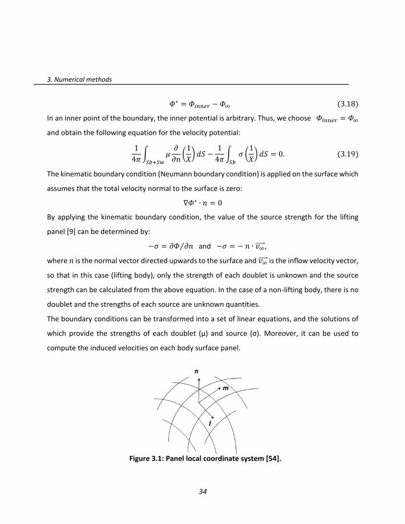
Figure 3.1: Panel local coordinate system [54].
.
l
n
m
3. Numerical methods
35
The induced velocities can be calculated on each panel as follows:
𝑣𝑖𝑛𝑑(𝑥 ) = (𝑣𝑙(𝑥 ) + 𝑣𝑚(𝑥 ))⏟ 𝑡𝑎𝑛𝑔𝑒𝑛𝑡𝑖𝑎𝑙 𝑐𝑜𝑚𝑝𝑜𝑛𝑒𝑛𝑡𝑠
+ 𝑣𝑛(𝑥 )⏟ 𝑛𝑜𝑟𝑚𝑎𝑙 𝑐𝑜𝑚𝑝𝑜𝑛𝑒𝑛𝑡𝑠
(3.20)
The tangential components are determined from the doublet distribution:
𝑣𝑙(𝑥𝑖) =−𝜕𝜇𝑖
𝜕𝜉, 𝑣𝑚(𝑥𝑖) =
−𝜕𝜇𝑖
𝜕𝜍 (3.21)
where 𝜉 and 𝜍 are the local tangential coordinates of the panel after calculating all velocity
components. The pressure distribution on each panel of the body can be completed by applying
the Bernoulli equation, which is defined as:
𝑝 + 𝜌𝑔𝑧 + 0.5𝜌𝑣2 + 𝜌 𝜕𝛷∗ 𝜕𝑡⁄ = 𝑐𝑜𝑛𝑠𝑡. (3.22)
The wake surface is a sheet of doublets, which is a thin layer without a displacement. The strength
is constant over one panel but can vary among each other in the case of unsteady flow. In order
to determine the induced velocities for the wake surface, the Kutta condition and the force-free
condition are applied.
The Kutta condition is applied at the trailing edge of the lifting body, at the point where the
vorticity leaves the surface it had been circulating around (closed and connecting body). In
accordance with Kelvin’s circulation theorem, the Kutta condition is a form of angular momentum
conservation [54] which states that the circulation’s time rate of change around a closed curve is
zero. The flow leaving the trailing edge of the airfoil is smooth, which means that the derivative
of the velocity potential at the airfoil trailing edge is finite:
∇𝛷𝑤(𝑡) < ∞ 𝑎𝑡 𝑡ℎ𝑒 𝑡𝑟𝑎𝑖𝑙𝑖𝑛𝑔 𝑒𝑑𝑔𝑒 (3.23)
The Kutta condition requires the jump of potentials at the trailing edge to convect the wake,
hence it is necessary to impose a pressure Kutta condition to ensure a zero pressure difference at
the trailing edge of the airfoil:
∆𝐶𝑃 = 𝐶𝑃+ + 𝐶𝑃
− (3.24)
The doublet strength of the wake surface behind the trailing edge can be calculated by using:

3. Numerical methods
36
𝜇𝑡.𝑒 = 𝜇𝑢𝑝𝑝𝑒𝑟 − 𝜇𝑙𝑜𝑤𝑒𝑟 (3.25)
Where 𝜇𝑢𝑝𝑝𝑒𝑟 and 𝜇𝑙𝑜𝑤𝑒𝑟 are the potentials on the upper and lower side of the airfoil’s trailing
edge. The doublet strength of each wake panel at the trailing edge is calculated at each time step.
According to the force-free condition, the flow field is history dependent on the wake surface
[58]. The strength on the shed wake is determined from the previous time step, meaning that the
current distributions of doublets on the wake surface depend on some previous distributions of
doublets. Therefore, the history of the motion is stored in the wake. The trailing wake sheet is
determined to satisfy the force-free condition, and modelled in unsteady manner.
3.1.3 Blade Tower Interaction
As wind turbine systems have become larger, investigating the interaction between the blade and
the tower has become increasingly more important for aerodynamic loading. However, there
exists a lack of studies describing this interaction. To investigate this case, the described
methodology is used to solve the flow around the rotor and tower in an iterative manner by
solving a two-equation system; the first one for the rotor and the second one for the tower. In
addition to considering the time-dependent effects of one component on the other, the
interactive effects of the components are taken into account by calculating the induced velocities
of each component on the other component at every time step. Figure 3.3 shows the flowchart
Figure 3.2: Wake sheet behind an airfoil.
.

3. Numerical methods
37
of solving the blade-tower interaction case by using an iterative procedure. In the first iteration
process, the tower problem is solved without the presence of the rotor. Next, the unsteady rotor
problem is solved by incorporating the unsteady tower-induced on rotor surface at the
corresponding time. The last two steps are repeated until the solution converges.
Yes
No
Yes
Start
Time=Time+dt
Solve tower problem
Add induced velocity of the
tower on the rotor
Solve rotor problem
Add induced velocity of the rotor on the tower
Converged solution
Time=Timemax
No
Print Results
Figure 3.3: Flowchart of blade-tower interaction procedure.
3. Numerical methods
38
3.1.4 Wave Generation Modelling
The wave potential is calculated according to the linear wave theory (Airy wave theory) [32]. The
estimated wave potential is superimposed onto other potentials present in the flow domain. The
potential function of a two-dimensional wave can be written as:
𝛷𝑊𝑎𝑣𝑒(𝑥, 𝑧, 𝑡) =𝐻𝑔
2𝜔ℯ𝑘𝑧 cos(𝜔𝑡 − 𝑘𝑥) (3.26)
Where 𝜔 denotes the wave angular frequency and 𝑘 the wave number equal to 2𝜋/𝜆. The waves
are propagating in the direction of the positive 𝑥-axis. The negative 𝑧-axis is pointing downwards
(in the water) and the level 𝑧 = 0 corresponds with the mean surface elevation. In order to
consider an arbitrary propagation direction (𝑦-axis), the previous equation can be modified with
a main wave direction 𝜓 :
𝛷𝑊𝑎𝑣𝑒(𝑥, 𝑦, 𝑧, 𝜓, 𝑡) =𝐻𝑔
2𝜔ℯ𝑘𝑧cos (𝜔𝑡 − 𝑘(𝑥 cos(𝜓) + 𝑦 sin(𝜓)) (3.27)
The wave velocity components 𝑢, 𝑣 and 𝑤 are the first derivative of the velocity potential with
respect to 𝑥, 𝑦 and 𝑧. Wind-generated waves in the real sea are generally multi-dimensional.
Therefore, a common approach is to represent the sea state by multi-dimensional waves
composed of an infinite number of regular waves with different frequencies and directions.
Various approaches have been proposed to estimate wave spectra properties. In the used solver
code, the JONSWAP spectrum is implemented. JONSWAP is an empirical relationship that defines
the distribution of the ocean wave energy over the angular frequency. To define the potential for
the irregular sea, a randomly chosen phase shift 𝜗𝑖between each elementary wave is introduced,
as well as the spectral dependency of the wave amplitude 𝐴𝑖:
𝛷𝑠𝑝𝑒𝑐𝑡(𝑥, 𝑧, 𝜓, 𝑡) = ∑𝐴𝑖𝑔
𝜔𝑖
𝐼𝑖=0 ℯ𝑘𝑖𝑧cos (𝜔𝑡 − 𝑘𝑥 + 𝜗𝑖) (3.28)

3. Numerical methods
39
|𝐴𝑖| = √2. 𝑆𝜁(𝜔𝑖)Δ𝜔𝑖 (3.29)
Where wave energy spectrum is 𝑆𝜁(𝜔𝑖) dependent on the frequency 𝜔𝑖 and the frequency band
width being Δ𝜔:
𝑆𝜁(𝜔) = 𝜌𝑔𝑆𝜁(𝜔𝑖)Δ𝜔 (3.30)
In order to give a tangible form for the spectra, the model is enlarged to link each wave’s direction
to the most probable direction, where the wave’s energy is dominated by the function Ρ(𝜓)𝑗:
𝑆𝜁(𝜔𝑖, 𝜓𝑗) = 𝑆𝜁(𝜔𝑖) ∗ Ρ(𝜓)𝑗 (3.31)
The wave energy is distributed over a range of directions [(𝜓0 −𝜋
2) , … , (𝜓0 +
𝜋
2)] and around
the main travel direction(𝜓0 ) by the functionΡ(𝜓). The two Ρ(𝜓) functions are implemented as
shown:
Ρ1(𝜓) =2
𝜋𝑐𝑜𝑠2 [(𝜓0 −
𝜋
2) ,… , (𝜓0 +
𝜋
2)]
Ρ2(𝜓) =8
3𝜋𝑐𝑜𝑠4 [(𝜓0 −
𝜋
2) ,… , (𝜓0 +
𝜋
2)]
(Ρ1) is used for the lower peak wave’s spectrum and ( Ρ2) for the higher peak wave’s spectrum in
order to illustrate the three-dimensional wave spectrum for 𝑖-number of elementary waves and
𝑗-number of travel directions, as described in Eq. (3.31):
𝛷𝑠𝑝𝑒𝑐𝑡(𝑥, 𝑦, 𝑧, 𝜓, 𝑡) =∑∑𝐴𝑖𝑔
𝜔𝑖
𝐽
𝑗=0
ℯ𝑘𝑖𝑧cos (𝜔𝑖𝑡 − 𝑘𝑖(𝑥 cos(𝜓𝑗) + 𝑦 sin(𝜓𝑗)) + 𝜗𝑖,𝑗)
𝐼
𝑖=0
(3.32)

3. Numerical methods
40
3.2 Finite Volume Method (RANSE solver)
For calculating the viscous flow, a RANSE-solver is applied to simulate the OWT in combination
with the SST turbulence model. The VOF method is also utilized for the computational domain
free surface detection. This section provides a detailed description of the solver and the other
models used in the simulations.
3.2.1 Governing Equations
General fluid flows are described by non-linear partial deferential equations known as the Navier-
Stokes equations, where the fluid flows are governed by the physical principles of the
conservation of mass, momentum, and energy. This system of equations consists of three
equations, two of them which are utilized in the simulation cases. The first equation, Eq. (3.33A),
called the continuity equation, is simplified to the incompressible case where 𝑢𝑖 denotes the
velocity in i-direction:
∇ 𝑢𝑖 = 0 (3.33A)
Assuming a Newtonian fluid type with constant viscosity, then the momentum equation [54] is
written as:
(𝜕𝑢𝑖𝜕𝑡+ 𝑢𝑖∇ 𝑢𝑖) 𝜌 = 𝜌𝑓𝑒 − ∇𝑝 + 𝜈. 𝜌 ∇
2 𝑢𝑖 (3.33B)
Where 𝑓𝑒 is a vector representing body forces. In order to contain the turbulence effects, time–
averaged and randomly fluctuating components can be used for each of the variables in the above
equations; [96] for instance, the velocity component will be:
3. Numerical methods
41
𝑢(𝒙, 𝑡) = (𝑥) + 𝑢′(𝒙, 𝑡) (3.34)
Where 𝑥 = (𝑥, 𝑦, 𝑧) is the position vector, is the time-averaged component and 𝑢′ the
fluctuating component. The time-averaged term is obtained by means of the Reynolds time-
average operator, which locally applied to the velocity vector reads as:
=1
Δ𝑡∫ 𝑢. 𝑑𝑡𝑡𝑜+Δ𝑡
𝑡𝑜
(3.35)
After applying the previous expression to the entire variable set in the Navier-Stokes equations,
the incompressible time-averaged Navier-Stokes equations result. Due to the nonlinearity of
these equations, their exact solution is generally difficult. Further, the solution is non-unique for
the given initial and boundary conditions [96], especially at the transition from laminar to
turbulent flow.
The turbulent flow is unsteady, three dimensional and takes place at a high Reynolds number. In
this kind of flow, the fluid inertia overcomes viscous forces and laminar flow loses its stability.
The non-linear, differential governing equations can be solved by applying a numerical method
to solve the flow field in a discrete manner. The numerical approach requires discrete descriptions
of space and time. Finite volume method is utilized for the space discretization: the computational
domain is divided into a number of smaller cells and the summation of these cells is the mesh.
Mesh generation is the first and an important step in CFD calculations and the simulations results
are heavily dependent on mesh quality.
After the discretization and applying the boundary condition, the general complicated equations
will convert into a system of algebraic equations and different iterative methods are used to solve
the algebraic equations.

3. Numerical methods
42
3.2.2 SST Turbulence Model
The shear-stress transport SST 𝑘 − 𝜔 model was developed by Menter [67] for flows with adverse
pressure gradients and separation. It has the ability to solve simultaneously the low Re (near-wall)
and high Re (far-field) zones, and to predict more accurately non-equilibrium regions in boundary
layer. A good example for adverse pressure gradients is the flow along the surface of an airfoil as
in Figure 3.4. Starting from the leading edge, the pressure decreases on the upper surface (suction
side) because the velocity increases. The pressure reaches its minimum at (x/c ≃ 0.15) and
increases after that due to velocity decreases. This region is called the adverse pressure gradient
region.
Figure 3.4: Color contour of pressure field around airfoil.
The 𝑘 − 𝜔 model is more accurate than the 𝑘 − 휀 model at predicting adverse pressure gradient
flow, so the SST model is a combination of 𝑘 − 휀 for the outer region and 𝑘 − 𝜔 for the near wall
region. While this approach makes the best use of 𝑘 − 𝜔 in the near wall region, it avoids the
sensitivity of this model to the free stream omega value. This can be neatly done by an
appropriate blending function that changes the model smoothly from 𝑘 − 𝜔 near the wall to 𝑘 −
휀. The two transport equations
3. Numerical methods
43
of the SST model are defined in [67]. An improved near-wall formulation used in this formulation
allows for reducing the near wall grid resolution requirements, meaning that the solutions are
insensitive to the 𝑌𝑝𝑙𝑢𝑠 value. Using SST in such a complicated case like wind turbines is convenient
because of the difficulties in achieving low 𝑦+ value.
3.2.3 Multiphase Modelling and Volume of Fluid Model
(VOF)
The multiphase flow regime, called free surface, is an interface between the water and the air. A
turbulence model is applied firstly for calculating the turbulent flow, which is the main focus in a
single-phase fluid simulation. Moreover, multiphase flow needs further modelling due to the
difficulties solving the interaction between the phases. Homogenous and inhomogeneous models
can be used for multiphase flow modelling.
An inhomogeneous model based on the Euler- Euler approach that treats all phases as continuous
is used. The phases are treated separately and the governing equations are solved for each phase.
In the homogenous approach, the time-averaged Navier-Stokes equation solves for mixture
properties, meaning all field variables are assumed to be shared between the two phases. The
free surface boundary can be detected in the computational domain using the VOF method and
a phase indicator function. A phase indicator function has the cell properties of volume of fraction
[6]. In each control volume, the sum of the volume fraction of all the phases equals one. For
instance, if the volume fraction of fluid in the cell is given as 𝛿, then its value will be 𝛿 = 0 if the
particular control volume does not contain this fluid. 𝛿 = 1 shows that the control volume is
entirely occupied by the fluid. 0 < 𝛿 < 1 shows this control volume contains the free surface
part. Based on the value of 𝛿, the properties of the flow variables are given in the volume-

3. Numerical methods
44
averaged flow equations. For example, the inlet velocity can be given according to the equation
below:
𝑢𝑖𝑛 = 𝑢𝑤𝑎𝑣𝑒 ∗ 𝛿𝑤𝑎𝑡𝑒𝑟 + 𝑢𝑎𝑖𝑟(1 − 𝛿𝑎𝑖𝑟) (3.36)

45
OWT Simulation Test Models
The objective of this chapter is to investigate the simulation models which are carried out using
BEM and RANS methods. These simulations have been conducted using three different
configurations (OWT rotor only, land wind turbine and monopile), which are regarded as a first
step toward simulating the combined aerodynamic and hydrodynamic loads on a full OWT.
This chapter is divided into two sections: the OWT aerodynamic simulations and the OWT
hydrodynamic simulations. The aerodynamic simulations first focus the rotor flow on its own, and
in a second case, then investigate the interaction between the flow of the tower and the rotor.
The geometry is presented first, followed by the solution steps and the details for the two solvers,
including mesh generation. These are followed by a comprehensive comparison between the two
methods results.
The hydrodynamic simulations cover the load on a slender cylinder in regular waves. This section
begins with a model description, followed by an explanation of the two solvers’ settings, and
concludes with a presentation of the results. For the validation of this case, the cylinder forces
calculated by the solvers are compared with the results obtained from the Morison equation.
The aim of these sections is to verify the wind turbine loads as well as to facilitate the
enhancement of both the simulation models and the tool settings. These simulations offer the
necessary foundation for further developing the coupling procedure between aerodynamic and
hydrodynamic OWT loads.

4. OWT simulation test models
46
4.1 Description of Model Designs
The NREL 5MW offshore wind turbine was chosen to be modeled due to the availability of the
geometry data [48]. The NREL offshore wind turbine is a modern wind turbine with a large scale
and a complex geometry shape. The structural model in this chapter contains a tower, nacelle
and rotor. The wind turbine rotor has three blades with a blade length of 61m. The blades are
attached to a hub with a radius of 2m, meaning the total rotor radius is 63m. The blade is
composed of several airfoil types, as shown in Figures 4.1 and 4.2, and their profiles are given in
different blade sections in Table 4.1. The first portion of the blade is a perfect cylinder; further
away from the root, a cylinder is smoothly blended into a series of DU (Delft University) airfoils.
In a distance of 44.55m away from the root, the NACA64 profile is used to define the blade shape
up to the tip.
The 3D geometry has been created using the in-house CAD code by implementing all the detail
configurations presented in Table 4.1 into a PFF file. This file contains all the blade details,
including all airfoil sections, the distance from the rotor center to every airfoil cross section, as
well as the twist angles in order to define the location where the blade-pitch axis passes through
each airfoil cross section. The location to pitch axis is defined as (AeroOrig + (0.25−AeroCent))
according to [7, 48].
Although the hub provides the structural support to the three blades, there is no adequate
information in the literature regarding the exact shape of the rotor hub. Therefore, in the present
work a typical geometry of the hub shape is developed. Since the area of the hub is relatively
small compared to the whole projection rotor area, using different hub shapes will have a minor
influence on the simulation results of the flow on the rotor blades.

4. OWT simulation test models
47
Figure 4.1: 2D Airfoil types used in the design of the wind-turbine blades.
Figure 4.2: 3D OWT blade airfoils.
DU-series NACA 64 Cylinder
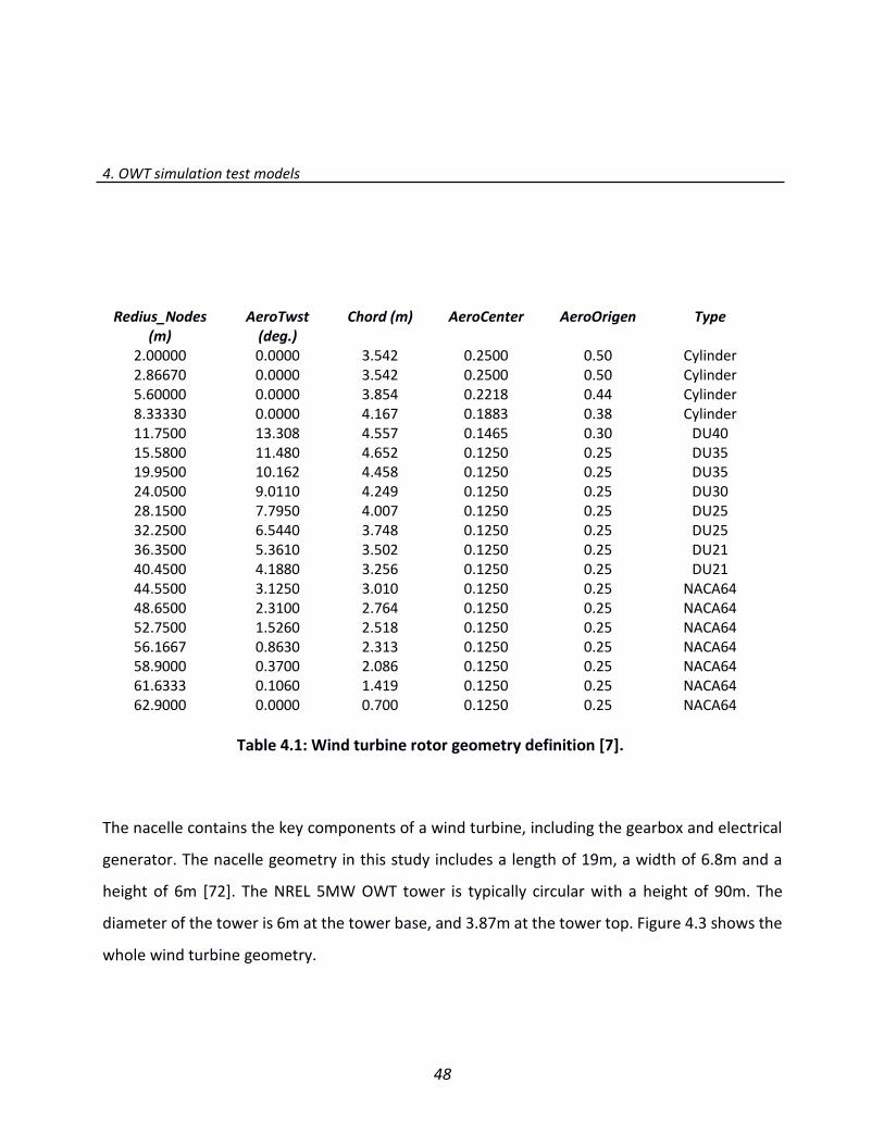
4. OWT simulation test models
48
Redius_Nodes (m)
AeroTwst (deg.)
Chord (m) AeroCenter AeroOrigen Type
2.00000 0.0000 3.542 0.2500 0.50 Cylinder 2.86670 0.0000 3.542 0.2500 0.50 Cylinder 5.60000 0.0000 3.854 0.2218 0.44 Cylinder 8.33330 0.0000 4.167 0.1883 0.38 Cylinder 11.7500 13.308 4.557 0.1465 0.30 DU40 15.5800 11.480 4.652 0.1250 0.25 DU35 19.9500 10.162 4.458 0.1250 0.25 DU35 24.0500 9.0110 4.249 0.1250 0.25 DU30 28.1500 7.7950 4.007 0.1250 0.25 DU25 32.2500 6.5440 3.748 0.1250 0.25 DU25 36.3500 5.3610 3.502 0.1250 0.25 DU21 40.4500 4.1880 3.256 0.1250 0.25 DU21 44.5500 3.1250 3.010 0.1250 0.25 NACA64 48.6500 2.3100 2.764 0.1250 0.25 NACA64 52.7500 1.5260 2.518 0.1250 0.25 NACA64 56.1667 0.8630 2.313 0.1250 0.25 NACA64 58.9000 0.3700 2.086 0.1250 0.25 NACA64 61.6333 0.1060 1.419 0.1250 0.25 NACA64 62.9000 0.0000 0.700 0.1250 0.25 NACA64
Table 4.1: Wind turbine rotor geometry definition [7].
The nacelle contains the key components of a wind turbine, including the gearbox and electrical
generator. The nacelle geometry in this study includes a length of 19m, a width of 6.8m and a
height of 6m [72]. The NREL 5MW OWT tower is typically circular with a height of 90m. The
diameter of the tower is 6m at the tower base, and 3.87m at the tower top. Figure 4.3 shows the
whole wind turbine geometry.
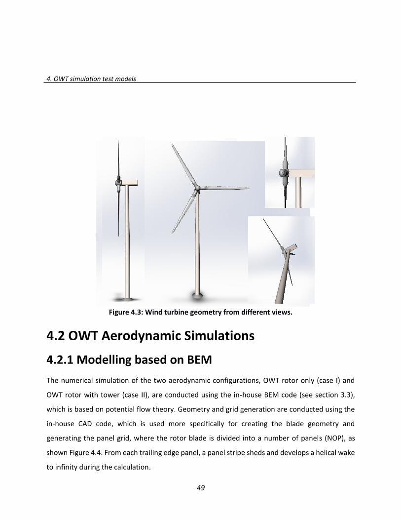
4. OWT simulation test models
49
4.2 OWT Aerodynamic Simulations
4.2.1 Modelling based on BEM
The numerical simulation of the two aerodynamic configurations, OWT rotor only (case I) and
OWT rotor with tower (case II), are conducted using the in-house BEM code (see section 3.3),
which is based on potential flow theory. Geometry and grid generation are conducted using the
in-house CAD code, which is used more specifically for creating the blade geometry and
generating the panel grid, where the rotor blade is divided into a number of panels (NOP), as
shown Figure 4.4. From each trailing edge panel, a panel stripe sheds and develops a helical wake
to infinity during the calculation.
Figure 4.3: Wind turbine geometry from different views.
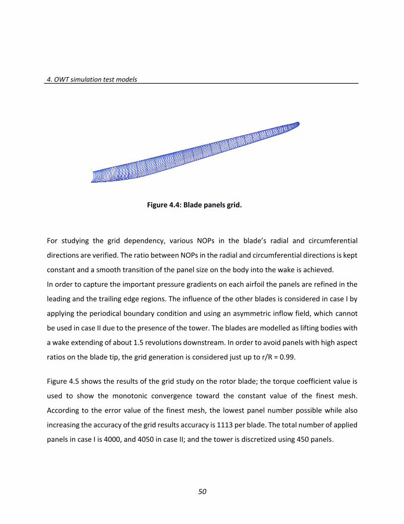
4. OWT simulation test models
50
For studying the grid dependency, various NOPs in the blade’s radial and circumferential
directions are verified. The ratio between NOPs in the radial and circumferential directions is kept
constant and a smooth transition of the panel size on the body into the wake is achieved.
In order to capture the important pressure gradients on each airfoil the panels are refined in the
leading and the trailing edge regions. The influence of the other blades is considered in case I by
applying the periodical boundary condition and using an asymmetric inflow field, which cannot
be used in case II due to the presence of the tower. The blades are modelled as lifting bodies with
a wake extending of about 1.5 revolutions downstream. In order to avoid panels with high aspect
ratios on the blade tip, the grid generation is considered just up to r/R = 0.99.
Figure 4.5 shows the results of the grid study on the rotor blade; the torque coefficient value is
used to show the monotonic convergence toward the constant value of the finest mesh.
According to the error value of the finest mesh, the lowest panel number possible while also
increasing the accuracy of the grid results accuracy is 1113 per blade. The total number of applied
panels in case I is 4000, and 4050 in case II; and the tower is discretized using 450 panels.
Figure 4.4: Blade panels grid.

4. OWT simulation test models
51
The rotor operation conditions includes a uniform wind speed at 11.4 m/sec with zero yaw angles,
and a rotational speed at 1.267 rad/sec, where the x-axis is the rotation axis and the z-y plane is
considered as the rotation plane, which gives a tip speed ratio of 7. The time of increment is
chosen such that the rotor blades advance 6.118 deg. at each time step. Therefore, one revolution
is completed in 5 seconds. Figure 4.7 shows the wake structure behind the wind turbine blades,
both excluding and including the presence of the wind turbine tower. The wake is shed from the
trailing edge of the rotor blades and is convicted downstream with the local fluid velocity.
Figure 4.5: Variation of the torque coefficient as a function of
the number of grid points.
.

4. OWT simulation test models
52
The Dirichlet boundary condition is applied in the simulation, which is initialized by steady
calculation iterations. The initial steady calculation is very important in predicting the wake
panel’s elementary location at which time is constant. This prior calculation is followed by
unsteady calculations, where at each time step, the free wake moves with the induced velocity
that is calculated at each panel. Each unsteady time step, or “explicit step”, involves a few implicit
steps (i.e. inner iterations), where the induced velocity is recalculated for each panel. In order to
avoid unstable fluctuations on the tower panel’s properties that would intersect with the wake
panel, a special technique is employed where all the wake panels inside and around the tower
are recognized and inactivated in the solution of the linear equation system.
Figure 4.6: Wake structure behind the wind turbine rotor.

4. OWT simulation test models
53
These intersected wake panels can be distinguished from other panels at each time step by
specifying a zero value for the split factor, and a one value for the others, as shown in Figure 4.7.
According to this factor, all the wake panels inside the blade-tower interaction region will be
excluded from the calculations by setting a zero value for its dipole strengths. It should be
mentioned that the strength of the dipoles, which have been saved before the collision, will be
reused again after passing the tower region, meaning it will not have any further effect on the
tower and rotor calculations.
4.2.2 Modelling based on RANSE
In this work, the commercial CFD code ANSYS CFX 14.5 is used to solve the viscous flow problem
on the same two geometry configurations used in the previous part by solving the
Figure 4.7: Wake split technique.
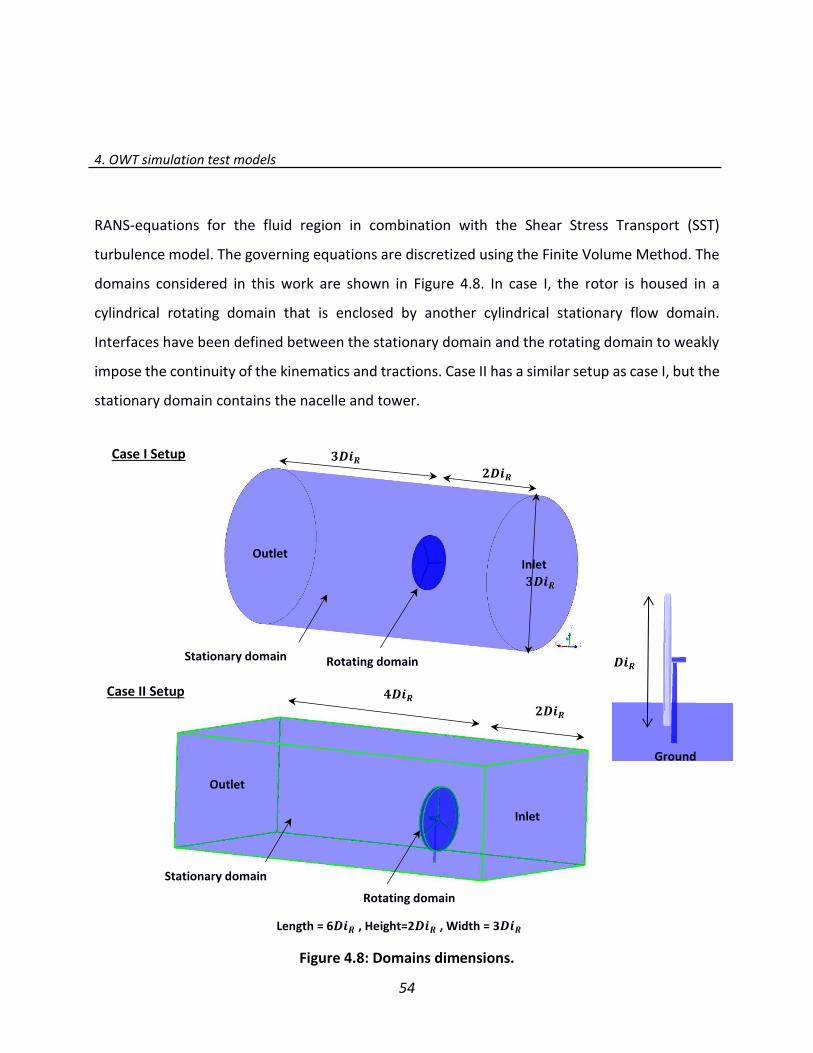
4. OWT simulation test models
54
RANS-equations for the fluid region in combination with the Shear Stress Transport (SST)
turbulence model. The governing equations are discretized using the Finite Volume Method. The
domains considered in this work are shown in Figure 4.8. In case I, the rotor is housed in a
cylindrical rotating domain that is enclosed by another cylindrical stationary flow domain.
Interfaces have been defined between the stationary domain and the rotating domain to weakly
impose the continuity of the kinematics and tractions. Case II has a similar setup as case I, but the
stationary domain contains the nacelle and tower.
Outlet Inlet
𝟑𝑫𝒊𝑹
𝟑𝑫𝒊𝑹
𝟐𝑫𝒊𝑹
Stationary domain Rotating domain
Case I Setup
𝑫𝒊𝑹
Ground
𝟒𝑫𝒊𝑹
𝟐𝑫𝒊𝑹
Outlet
Inlet
Stationary domain
Rotating domain
Length = 6𝑫𝒊𝑹 , Height=2𝑫𝒊𝑹 , Width = 3𝑫𝒊𝑹
Case II Setup
Figure 4.8: Domains dimensions.
.

4. OWT simulation test models
55
4.2.2.1 Mesh Generation
Mesh generation is the first important step towards obtaining the right CFD solution as an
optimum grid facilitates the convergence to the correct results. The most common types of grids
are structured and unstructured grids. Structured mesh has a higher metrics quality but a lower
degree of adaptability to complex geometries; while unstructured meshes are more flexible with
respect to geometrical topology and therefore are used for the wind turbine blades, which have
a complex geometry.
ANSYS ICEM CFD is chosen for mesh generation due to its ability to generate different types of
meshes with different algorithms. The surface mesh type is a triangle with a maximum size
element of 0.4m2 and a maximum deviation of 0.01, where the use of such low deviation values
allows for subdividing the element surface on the center of a triangle element, meaning that the
mesh deform around the surface is of a higher quality. Figure 4.9 shows the surface mesh around
the blade.
Tetrahedral elements are chosen for the flow volume domain. Figure 4.10 shows the 2D plane
mesh at x-y plane for case I and x-z plane for the second case, where the mesh refined in the
inner region allows for better flow resolution near the rotor. Prismatic elements are used for
creating layers around the blade surface in order to have a mesh in proximity of the boundary
layer. The applied hybrid tetrahedral mesh includes layers of prism elements near the wall
boundary surfaces and the tetrahedral elements in the interior region. Such a hybrid concept
allows for the mesh to become progressively coarser since the flow gradients approach zero in
the outer flow.
Figure 4.9: Surface mesh on the blade.

4. OWT simulation test models
56
The used prism-meshing layer has elements perpendicular to the surface, making it possible to
keep the 𝑦+ value nearly constant over the wall regions. Figure 4.11 illustrates a 2D section of
the blade boundary-layer mesh. The resulting boundary-layer mesh for each blade consists of 20
layers, where the first-layer thickness is about 2.0×10⁻³ m and the growth ratio is 1.2.
Case I
x-y plane
Rotating domain
Case II
x-z plane
Figure 4.10: Stationary and rotating domains volume mesh.
Stationary domain

4. OWT simulation test models
57
Inlet region Inlet boundary condition
Outlet and sides Opening boundary condition
Blades, tower, nacelle and Bottom No-slip wall
Case I number of elements 10.218 Million
Case II number of elements 11.326 Million
Figure 4.11: Boundary layer mesh at 𝒓/𝑹 = 0.65.
.
Figure 4.12: 𝒚+ values around the blade.
Table 4.2: Boundary conditions for case I and case II.

4. OWT simulation test models
58
Due to near wall refinement, the maximum calculated 𝑦+ at this simulation is 200, as shown in
Figure 4.12. Finally, the total number of elements in case I and case II are about 10.218 and 11.326
million cells, respectively, as shown in Table 4.2. The next step is to define the boundary
conditions for the entire domain. First, at the inlet boundary, a uniform wind speed of 11.4 m/sec
and the physical properties of air at 25 𝐶𝑜 are defined. At the outlet, an opening boundary
condition is applied, which means the flow can exit or enter through this boundary surface. The
static pressure value is specified at the outlet boundary. The pressure is set to zero so that the
pressure at the outlet is equal to the atmospheric pressure at sea level (101,325 Pa).
The opening boundary condition is also applied on the side boundaries in case I and in case II as
well as the top boundaries in case II of the computation domain. No-slip boundary condition is
applied on the wall of the blades, tower, nacelle and ground, where the normal fluid velocity at
the body surface has a zero value.
In order to solve the transient problems, the initial conditions in both stationary rotating domains
are specified. For the stationary domain, a parallel inflow velocity of 11.4 m/sec is applied. For
the rotating domain, an angular velocity of 12.1 rev/min is defined. The selected time step is
0.02778 sec, which corresponds to a blade rotation of 2.0°.
4.2.3 Results and Validation
The results of both methods are compared in this section. All computations consider the same
free stream velocity and rotor rotating speed. The computation using the RANSE solver is carried
out employing 32 processors of an in-house cluster, with 2.2 GHz for each processor and 121.7
GB of memory. The CPU time is thus 96 and 104 hours for case I and case II respectively. The BEM
solver uses 4 processors with 3.3 GHz for each processor and 7 GB of memory. The CPU time is
thus 12 hours for the first case and 24 hours for the second.
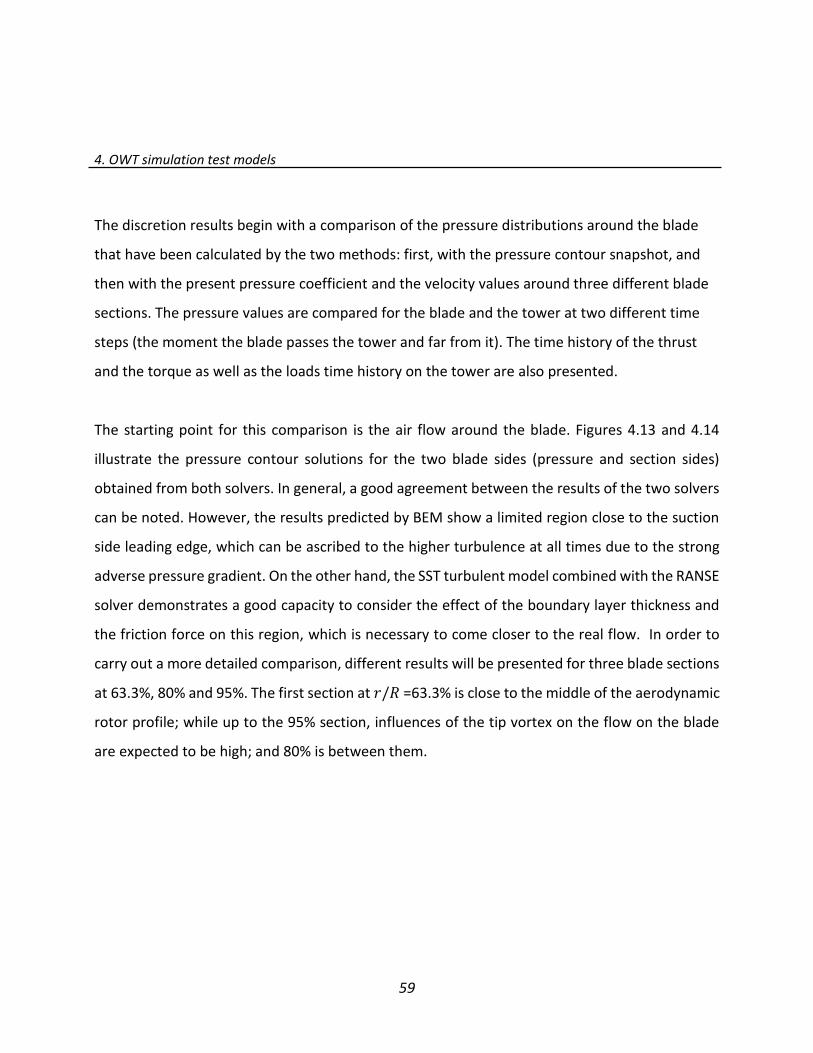
4. OWT simulation test models
59
The discretion results begin with a comparison of the pressure distributions around the blade
that have been calculated by the two methods: first, with the pressure contour snapshot, and
then with the present pressure coefficient and the velocity values around three different blade
sections. The pressure values are compared for the blade and the tower at two different time
steps (the moment the blade passes the tower and far from it). The time history of the thrust
and the torque as well as the loads time history on the tower are also presented.
The starting point for this comparison is the air flow around the blade. Figures 4.13 and 4.14
illustrate the pressure contour solutions for the two blade sides (pressure and section sides)
obtained from both solvers. In general, a good agreement between the results of the two solvers
can be noted. However, the results predicted by BEM show a limited region close to the suction
side leading edge, which can be ascribed to the higher turbulence at all times due to the strong
adverse pressure gradient. On the other hand, the SST turbulent model combined with the RANSE
solver demonstrates a good capacity to consider the effect of the boundary layer thickness and
the friction force on this region, which is necessary to come closer to the real flow. In order to
carry out a more detailed comparison, different results will be presented for three blade sections
at 63.3%, 80% and 95%. The first section at 𝑟/𝑅 =63.3% is close to the middle of the aerodynamic
rotor profile; while up to the 95% section, influences of the tip vortex on the flow on the blade
are expected to be high; and 80% is between them.
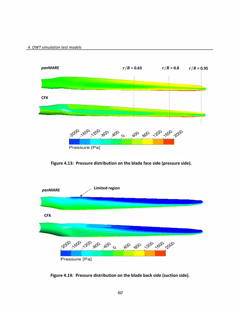
4. OWT simulation test models
60
Figure 4.13: Pressure distribution on the blade face side (pressure side).
.
𝒓/𝑹 = 0.95 𝒓/𝑹 = 0.8 𝒓/𝑹 = 0.63
CFX
panMARE
Figure 4.14: Pressure distribution on the blade back side (suction side).
Limited region panMARE
CFX
4. OWT simulation test models
61
Figure 4.15 shows pressure coefficient distributions for the three 2D blade sections against a
normalized chord. The upper and the lower parts show the pressure distribution on the pressure
and suction side of the section, respectively. The non-dimensional pressure coefficient is plotted
for the sections over the non-dimensional chord length using the following formula:
𝐶𝑝 = (𝑝 − 𝑝∞)/(0.5𝜌∞[𝑣∞2 + (Ω𝑟)2] ) (4.1)
While the lift coefficient of the section depends directly on the pressure coefficient, the drag
coefficient is strongly influenced by the separated flow. The stagnation pressure value at the tip
of the leading edge ( 𝑥
𝑐 = 0) is higher than the middle and root sections. The formula (4.1) allows
for the normalization of the stagnation pressure for all sections to a value that equals 1. A good
agreement between the results of the two applied solvers can be seen on the pressure side (upper
curve) where the pressure is almost positive. At the suction side (bottom) the pressure until 0.3c
has the lowest value and after this region, the pressure increases to the value at the trailing edge.
The comparison of the pressure coefficient values show the capability of BEM to predict the
pressure distribution on different blade airfoils. The velocity on the blade sections is shown along
streamlines for the investigated angle of attack, as seen in Figure 4.16. The flow over the blade
appears largely attached at all sections. However, there is a separation flow in boundary layer at
the trailing edge, where the maximum velocity of the reversal flow increases with increasing angle
of attack and Re number.

4. OWT simulation test models
62
Figure 4.15: Pressure coefficient distributions at different blade sections.
𝑟 𝑅⁄ = 0.8
𝑟 𝑅⁄ = 0.6
𝑟 𝑅⁄ = 0.95
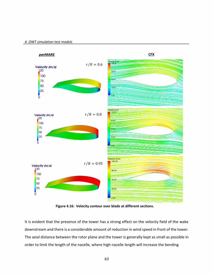
4. OWT simulation test models
63
It is evident that the presence of the tower has a strong effect on the velocity field of the wake
downstream and there is a considerable amount of reduction in wind speed in front of the tower.
The axial distance between the rotor plane and the tower is generally kept as small as possible in
order to limit the length of the nacelle, where high nacelle length will increase the bending
Figure 4.16: Velocity contour over blade at different sections.
panMARE CFX
𝑟 𝑅⁄ = 0.6
𝑟 𝑅⁄ = 0.8
𝑟 𝑅⁄ = 0.95

4. OWT simulation test models
64
moments induced by the rotor blades on the tower. On the other hand, a smaller distance
between rotor and tower increases the aerodynamic interaction between flow around the tower
and the rotor blades.
The up-wind rotor is affected by a reduction of the flow in front of the tower. This reduction is an
important factor and can lead to a strong change in the rotor blade’s effective aerodynamic angle
of attack and a sudden change of the lift force on the rotor blade. It strongly affects both the
aerodynamic loading on the wind turbine rotor and tower. The actual 5MW wind turbine uses
blades with increasing tower clearance without a large rotor overhang. Therefore, precone and
tilt angle are used in the baseline wind turbine [48].
Figures 4.17 and 4.18 show pressure distributions from both solvers at spanwise cross section
80% from the rotating blades, which have different angular positions relative to the tower. The
first blade has 120 degrees relative to the tower and the second blade is in front of the tower.
The results of both simulation methods show a clear reduction in the aerodynamic loads. The
value of the pressure suffers a drop on the suction side of the second blade. In the investigation
of the interaction effect on the tower when the blades just pass the tower, the horizontal forces
acting on the tower experience a sudden decrease due to the reduction of the pressure
distribution on one side of the tower. This reduction is induced by free vortex shaded from the
rotating blade as well as from the pressure field around the blade surface.
The rotor influence on the tower is illustrated in Figure 4.19 (A to C), which shows the tower
pressure distribution when the blade has 0 degree angle from the tower’s center line. Figure 4.20
(A to C) presents the tower pressure distribution when the blade has 60 degrees from the tower’s
center line. (A) and (B) show a good agreement between the results of the two solvers for the
pressure distribution at the different blade positions. (C) contains a comparison of the pressure
distribution on the tower leading edge (stagnation values) for both cods. As can be seen, the
pressure decreases on the tower leading edge when the blade passes the tower. This sudden drop
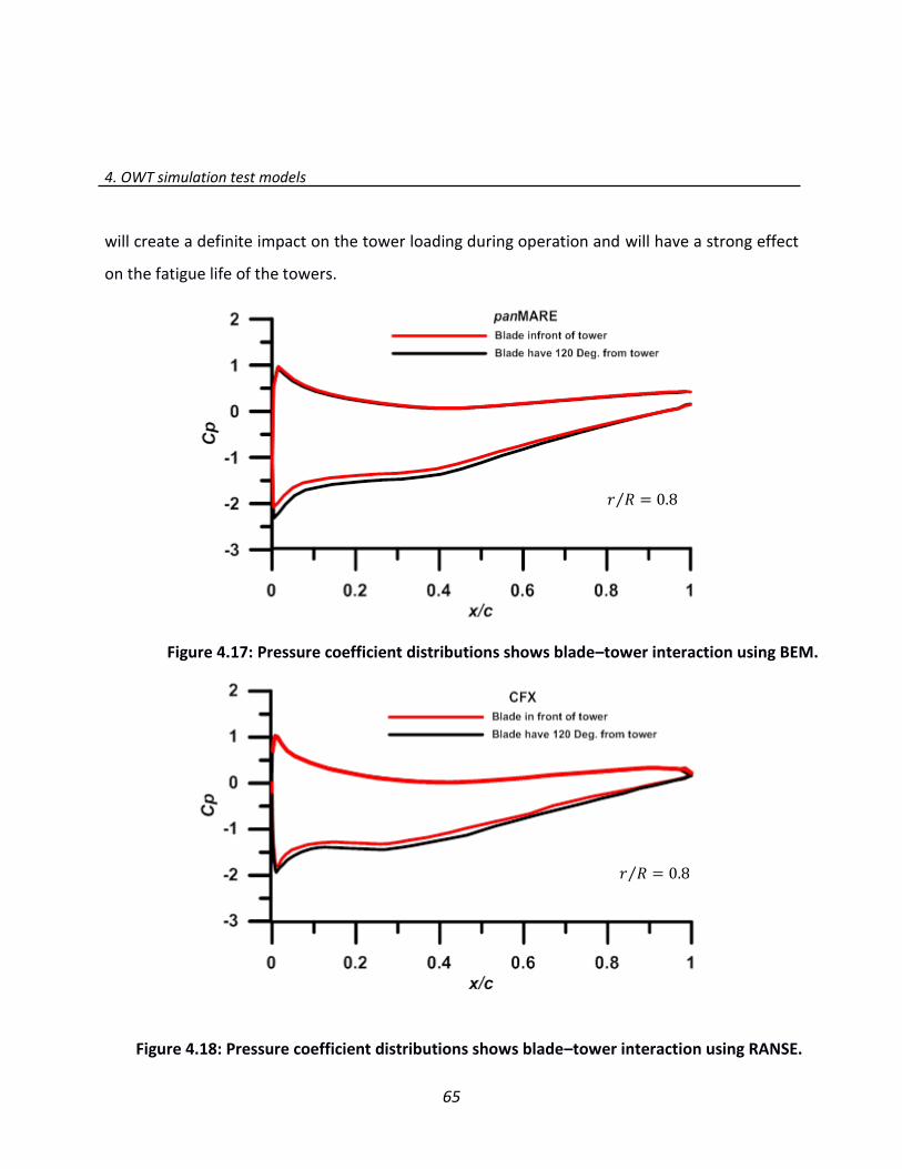
4. OWT simulation test models
65
will create a definite impact on the tower loading during operation and will have a strong effect
on the fatigue life of the towers.
Figure 4.18: Pressure coefficient distributions shows blade–tower interaction using RANSE.
Figure 4.17: Pressure coefficient distributions shows blade–tower interaction using BEM.
𝑟 𝑅⁄ = 0.8
𝑟 𝑅⁄ = 0.8

4. OWT simulation test models
66
Figure 4.20: Pressure distribution on the tower when the blade has 60o from tower:
A. CFX B. panMARE C. On tower leading edge for both codes.
(A) (B)
Figure 4.19: Pressure distribution on the tower when the blade has 0o from tower: A. CFX B. panMARE C. On the tower leading edge for both codes.
(B) (A) (C)
(C)

4. OWT simulation test models
67
The unsteady nature of the flow, due to the unsteady interaction between rotor and tower, is
simulated for a period of 20 sec, which corresponds to 4 revolutions, in order to reach a perodic
solution. state. Figure 4.21 shows the time history of the thrust and torque for the rotor for both
case I and case II (with and without presence of tower) at the desired rotation axis. The rotor
develops a favorable aerodynamic torque with both methods, which can generate 5 MW [8, 48].
The objective of the present simulations is to estimate the maximum torque value with each
simulation method in order to show that the meshing and the methods employed here can be
used to characterize the temporal and spatial natures of the flow loads near the rotor.
As can be seen in case ll, thrust and torque values show periodical behavior due to the blade-tower
interaction where every peak refers to one blade passing in front of the tower. The main thrust
value as well as the amplitude of the thrust oscillation obtained by BEM are slightly higher than the
results of RANSE. Additionally, the RANSE solver needs two revolutions for an accurate results
prediction.
Figure 4.22 shows the time history of the force on the tower in the flow direction (x-direction).
Both computational methods predict nearly the same amplitude and force fluctuations. Multi-
peaks for the force history curve are observed, which are related to the blade passing in front of
the tower. The strong wake effects on the tower force predicted by the BEM take place directly
after the blade passes, i.e. where the maximum force takes place. This high force is reduced after
wake sheet crosses the tower. The tower forces behavior is due to the wake singularity
assumption in the BEM code. On the other hand, different force behaviors are obtained from the
RANSE solver where the rotor wake has different effects. Furthermore, due to the cylindrical
shape of the tower a large separated flow region must be expected. The separated flow region
and its influence on the tower forces cannot be predicted by the panel method, so tower forces
in the lateral axis cannot be compared.
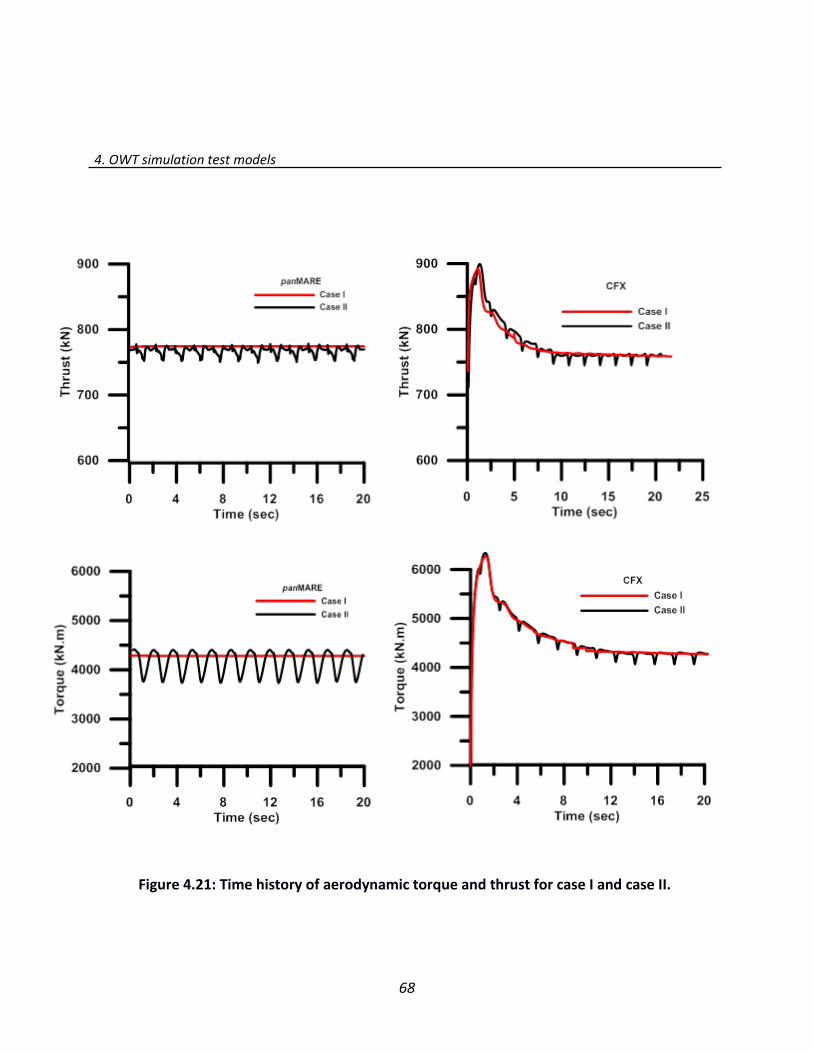
4. OWT simulation test models
68
Figure 4.21: Time history of aerodynamic torque and thrust for case I and case II.
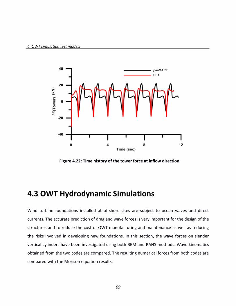
4. OWT simulation test models
69
4.3 OWT Hydrodynamic Simulations
Wind turbine foundations installed at offshore sites are subject to ocean waves and direct
currents. The accurate prediction of drag and wave forces is very important for the design of the
structures and to reduce the cost of OWT manufacturing and maintenance as well as reducing
the risks involved in developing new foundations. In this section, the wave forces on slender
vertical cylinders have been investigated using both BEM and RANS methods. Wave kinematics
obtained from the two codes are compared. The resulting numerical forces from both codes are
compared with the Morison equation results.
Figure 4.22: Time history of the tower force at inflow direction.
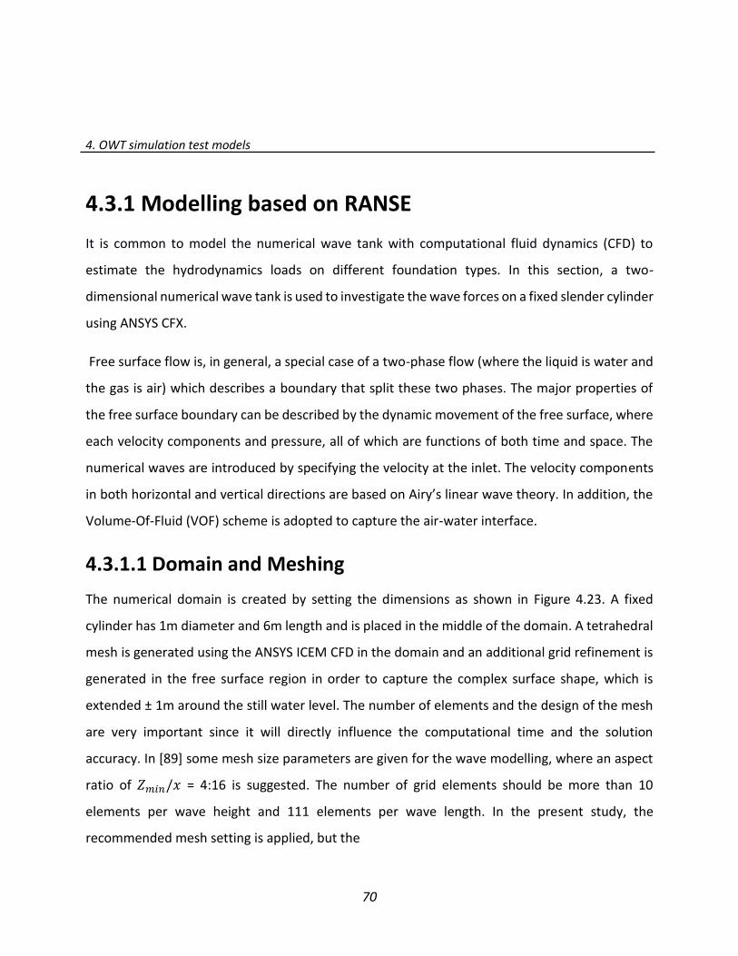
4. OWT simulation test models
70
4.3.1 Modelling based on RANSE
It is common to model the numerical wave tank with computational fluid dynamics (CFD) to
estimate the hydrodynamics loads on different foundation types. In this section, a two-
dimensional numerical wave tank is used to investigate the wave forces on a fixed slender cylinder
using ANSYS CFX.
Free surface flow is, in general, a special case of a two-phase flow (where the liquid is water and
the gas is air) which describes a boundary that split these two phases. The major properties of
the free surface boundary can be described by the dynamic movement of the free surface, where
each velocity components and pressure, all of which are functions of both time and space. The
numerical waves are introduced by specifying the velocity at the inlet. The velocity components
in both horizontal and vertical directions are based on Airy’s linear wave theory. In addition, the
Volume-Of-Fluid (VOF) scheme is adopted to capture the air-water interface.
4.3.1.1 Domain and Meshing
The numerical domain is created by setting the dimensions as shown in Figure 4.23. A fixed
cylinder has 1m diameter and 6m length and is placed in the middle of the domain. A tetrahedral
mesh is generated using the ANSYS ICEM CFD in the domain and an additional grid refinement is
generated in the free surface region in order to capture the complex surface shape, which is
extended ± 1m around the still water level. The number of elements and the design of the mesh
are very important since it will directly influence the computational time and the solution
accuracy. In [89] some mesh size parameters are given for the wave modelling, where an aspect
ratio of 𝑍𝑚𝑖𝑛/𝑥 = 4:16 is suggested. The number of grid elements should be more than 10
elements per wave height and 111 elements per wave length. In the present study, the
recommended mesh setting is applied, but the
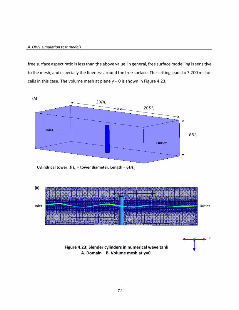
4. OWT simulation test models
71
free surface aspect ratio is less than the above value. In general, free surface modelling is sensitive
to the mesh, and especially the fineness around the free surface. The setting leads to 7.200 million
cells in this case. The volume mesh at plane y = 0 is shown in Figure 4.23.
20𝐷𝑖𝑐
20𝐷𝑖𝑐
8𝐷𝑖𝑐
Cylindrical tower: 𝑫𝒊𝒄 = tower diameter, Length = 6𝑫𝒊𝒄
Inlet
Outlet
Inlet Outlet
(A)
(B)
Figure 4.23: Slender cylinders in numerical wave tank A. Domain B. Volume mesh at y=0.
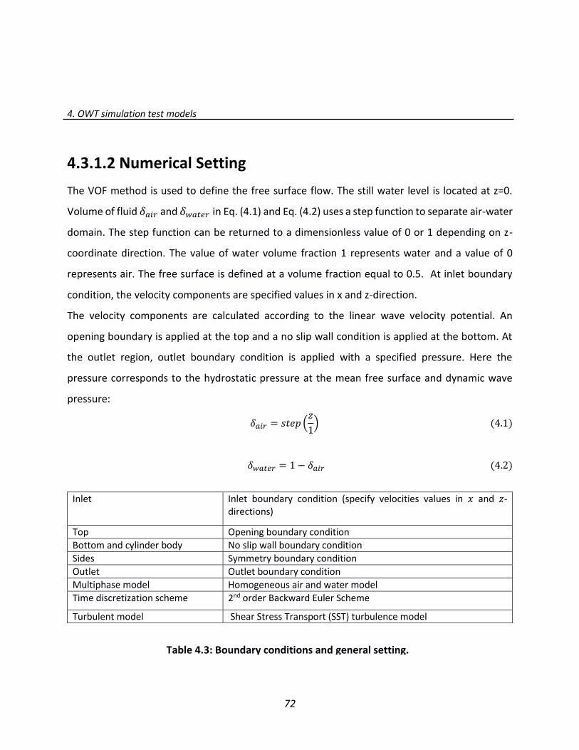
4. OWT simulation test models
72
4.3.1.2 Numerical Setting
The VOF method is used to define the free surface flow. The still water level is located at z=0.
Volume of fluid 𝛿𝑎𝑖𝑟 and 𝛿𝑤𝑎𝑡𝑒𝑟 in Eq. (4.1) and Eq. (4.2) uses a step function to separate air-water
domain. The step function can be returned to a dimensionless value of 0 or 1 depending on z-
coordinate direction. The value of water volume fraction 1 represents water and a value of 0
represents air. The free surface is defined at a volume fraction equal to 0.5. At inlet boundary
condition, the velocity components are specified values in x and z-direction.
The velocity components are calculated according to the linear wave velocity potential. An
opening boundary is applied at the top and a no slip wall condition is applied at the bottom. At
the outlet region, outlet boundary condition is applied with a specified pressure. Here the
pressure corresponds to the hydrostatic pressure at the mean free surface and dynamic wave
pressure:
𝛿𝑎𝑖𝑟 = 𝑠𝑡𝑒𝑝 (𝑧
1) (4.1)
𝛿𝑤𝑎𝑡𝑒𝑟 = 1 − 𝛿𝑎𝑖𝑟 (4.2)
Inlet Inlet boundary condition (specify velocities values in 𝑥 and 𝑧-directions)
Top Opening boundary condition
Bottom and cylinder body No slip wall boundary condition
Sides Symmetry boundary condition
Outlet Outlet boundary condition
Multiphase model Homogeneous air and water model
Time discretization scheme 2nd order Backward Euler Scheme
Turbulent model Shear Stress Transport (SST) turbulence model
Table 4.3: Boundary conditions and general setting.

4. OWT simulation test models
73
The domain sides are considered to be symmetrical planes. Homogeneous and inhomogeneous
models can be used in CFX to simulate multiphase flows like air and water. In this study, the
homogeneous model with a coupled solver is used in combination of a fully implicit scheme,
where the same flow fields (such as velocity and pressure) are shared by all fluids and the
momentum equations are set for the two phases for one time at each time step. Therefore, fewer
amounts of iterations are required for convergence in the steady and transient simulations [6].
The 2nd-order Backward Euler Scheme is applied with 10−5 convergence criteria and the number
of coefficient loops sets from 3 to 6 loops in each time step. Isothermal heat transfer and
buoyancy is used. In this case study, the wave length is 15m, the water depth is 4m and the ratio
(𝑑/𝜆) is less than 0.5. Waves are thus generated in an intermediate water depth for an angular
frequency of 𝜔 = 1.955 rad/s. The wave steepness of 𝐻/𝜆 = 0.033 is well below the breaking
criteria; and according to the value of the ratio (𝐷𝑖/𝜆 =0.066), the case cylinder is regarded as a
hydro-dynamically transparent structure (slender structure), meaning that diffraction and
reflection phenomena are negligible.
4.3.2 Modelling based on BEM
The potential flow around a slender cylinder with a 1m diameter is simulated using BEM with the
same wave height of 0.5m and wave period of 3.2139sec. This code description is given in chapter
3. The 2D wave which based on linear wave theory is used to estimate wave kinematics. The
influence of the presence of the cylinder is not taken into account in the wave kinematics
calculation. The induced velocity calculated from the solver due to the presence of the cylinder is
superimposed on the wave kinematics to estimate the total induced velocity.
The cylinder is discretized using the in-house CAD code with 60 panels in the vertical direction
and 40 in the radial direction. The panels are refined on the free surface region, as shown in Figure
4.24.

4. OWT simulation test models
74
The hydrodynamic force is calculated for the actual immersion of the body surface, so the
immersion of the panels are considered in each time step and all the panels located above the
free surface are excluded from the solution. A split factor is used for the fully or partially
immersed panel by consideration of the body-induced potential, as shown in Figure 4.25. Further,
the influence of partly immersed panels is considered by reducing their source and dipoles
strengths according to the immersed panel area ratio in [27]. Hydrodynamic forces on a circular
cylinder in waves can be estimated by integrating the pressure on the immersed surface body.
For verification of the applied methods, the numerical results obtained from the two methods
are compared with the Morison equation results.
Figure 4.24: CAD grid discretization.
.

4. OWT simulation test models
75
4.3.3 Hydrodynamic Loads Based on Morison Equation
In this section Airy wave theory, which is based on potential flow theory, is used to describe the
motion of gravity waves on the fluid and Morison equation utilized to calculate the hydrodynamic
load in time domain. This equation combines the linear inertia forces arising from fluid particle
acceleration with the nonlinear drag force arising from the wave effects.
Elements
Nodes
Nodes
Figure 4.25: Wave split technique.
.
Figure 4.26: Geometry definitions.
4. OWT simulation test models
76
Figure 4.27 represents the flowchart procedure of the implemented program, where the
hydrodynamic loads on offshore wind foundation are, in principle, determined by a three-step
procedure. First, the pre-calculation step, where the foundation geometry can be defined to a
certain member of elements and each element is defined by two nodes as shown in figure 4.26.
The input file of the program includes the element number, body node coordinates and the wave
properties. The calculations are done for each element in duration the calculation time.
The solution starts in the second step, where in each element many nodes are created in between
the main two nodes. The wave induced flow velocity and acceleration components are estimated
at each node. Using additional nods allows for a more accurate computation of each element.
The wave kinematics are calculated with respect to the general global coordinate system and then
transferred to the local element coordinate system. In the third step, the Morison equation is
applied to calculate the forces at each node. It should be mentioned that the considered
theoretical value for the coefficient 𝐶𝐷 and 𝐶𝑀 are selected according to ref. [44], which depend
on the values of Reynolds and Keulegen-Carpenter numbers. The mean value of the node forces
in each element and the total system load are determined for each time step. The total
hydrodynamic force is the summation of all the forces on the foundation elements.
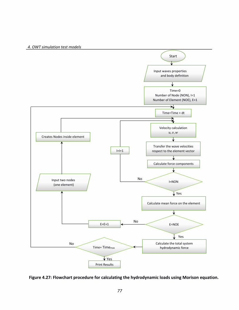
4. OWT simulation test models
77
Figure 4.27: Flowchart procedure for calculating the hydrodynamic loads using Morison equation.
Yes
No
No
Start
Time=0
Number of Node (NON), I=1
Number of Element (NOE), E=1
Yes
Input waves properties
and body definition
Time=Time + dt
Velocity calculation
𝑢, 𝑣, 𝑤
Yes
No
Transfer the wave velocities
respect to the element vector
Calculate force components
I=NON
Calculate mean force on the element
Time= Timemax Calculate the total system
hydrodynamic force
E=NOE E=E+1
Print Results
Input two nodes
(one element)
Creates Nodes inside element
I=I+1
4. OWT simulation test models
78
4.3.4 Results Comparison
According to 1st-order wave theory, the energy of a wave may reach the outlet region in 8.56sec
with a phase velocity of 4.67 m/sec. However, a longer simulation time of more than 20sec is
chosen to verify the behavior of the free surface. First, the calculated wave kinematics are
compared between the two solvers. Figure 4.28 shows the surface elevations at a specified point
located on the free surface about two meters in front of the cylinder surface. The very good
agreement between the results of both solvers indicates that the boundary conditions and the
solvers setting are reasonable. The horizontal and vertical water velocity components are shown
in Figures 4.29 and 4.30. The comparison shows a good agreement of the vertical velocity
component and very small deviation of the horizontal velocity component.
In Figure 4.31, the dynamic wave pressure at the studied point for the two solvers are compared,
and shows a small variation. The dynamic pressure is determined by subtracting the hydrostatic
pressure value from the total pressure estimated at the studied point. The errors calculated with
respect to the exact wave solution of the overall wave kinematics are shown in Table 4.4, where
the maximum error is 4.53%. Figure 4.32 presents the time history of the hydrodynamic loads on
the cylinder along the wave propagation direction, which are calculated using the two methods
and compared with the results obtained from the Morison equation. The mean loads for the last
encountered three wave amplitude value can be seen in Table 4.5 and its difference with respect
to the Morison equation results, where 8 % is the maximum error obtained. It should be
mentioned that for RANSE solver, the cylinder loads after 21sec are not taken into consideration
in order to avoid output region reflection.
The calculated differences are low and are associated with many numerical and physical aspects
involved in the calculation. In RANS method, the hydrodynamic force acting on the cylinder are
calculated by considering the general governing equation for the fluid behavior. Therefore, the
total hydrodynamic forces contain both pressure and viscous forces.
4. OWT simulation test models
79
The pressure force is an integration of the pressure on the area of the studied region and the
viscous friction forces is an integration of the shear stress on the same region. In other words, the
inertia and drag forces on the cylinder are calculated.
BEM depends on potential method to calculate the hydrodynamic loads, where viscous effects
are not present. The total hydrodynamic forces on the cylinder calculated using this solver contain
the inertia force without any estimation of the drag force. The body effect on the wave are also
not considered in the wave kinematics calculation.
The Morison equation calculates both the inertia and drag forces. The coefficients of drag and
inertia are chosen according to reference [44], where 𝐶𝐷=1 and 𝐶𝑀=2, respectively. In the study,
the non-dimensional parameters set by the Keulegan-Carpenter number (KC) and Re number are
1.55 and 5 ∗ 105, respectively. The Keulegan-Carpenter number describes the contribution of
the drag force to the total force, where the inertia forces dominate at the low value of the
Keulegan-Carpenter number (less than 0.5) and the drag forces dominate at the Keulegan-
Carpenter number of more than 40. Between these values each of these forces contribute to the
total force [5], while the Re numbers indicate the laminar flow status. According to the analysis
above, the contribution of inertia force is much greater than drag force in this case.
Further, it is clear from Figure 4.32 that the RANSE solver can capture the wave periodic behavior
only after one wave period, but other results shows symmetrical periodic behavior from the
beginning of calculation. The forces calculated by the Morison equation are higher than those
calculated by the RANS and BEM methods. While the RANSE solver appears to give more realistic
results than the BEM solver, but the difference is acceptable, according to the above results, the
BEM solver can obtain an accurate hydrodynamic forces and this code is more economical than
the RANSE solver.
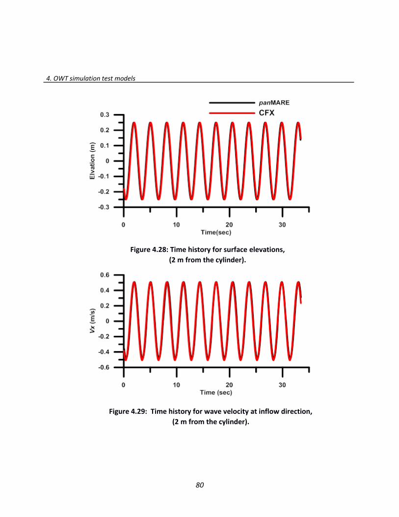
4. OWT simulation test models
80
Figure 4.28: Time history for surface elevations,
(2 m from the cylinder).
Figure 4.29: Time history for wave velocity at inflow direction,
(2 m from the cylinder).

4. OWT simulation test models
81
Figure 4.30: Time history for wave velocity at vertical direction,
(2 m from the cylinder).
Figure 4.31: Time history for wave dynamic pressure, (2 m from the cylinder).
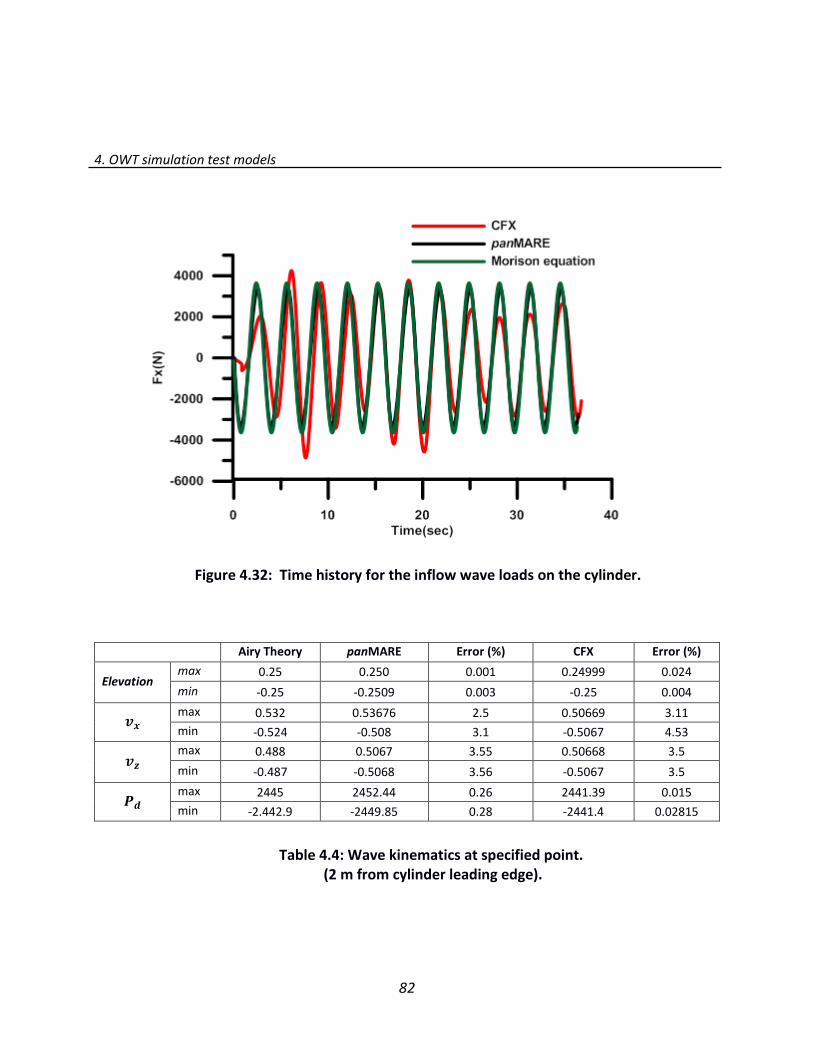
4. OWT simulation test models
82
Airy Theory panMARE Error (%) CFX Error (%)
Elevation max 0.25 0.250 0.001 0.24999 0.024
min -0.25 -0.2509 0.003 -0.25 0.004
𝒗𝒙 max 0.532 0.53676 2.5 0.50669 3.11
min -0.524 -0.508 3.1 -0.5067 4.53
𝒗𝒛 max 0.488 0.5067 3.55 0.50668 3.5
min -0.487 -0.5068 3.56 -0.5067 3.5
𝑷𝒅 max 2445 2452.44 0.26 2441.39 0.015
min -2.442.9 -2449.85 0.28 -2441.4 0.02815
Figure 4.32: Time history for the inflow wave loads on the cylinder.
Table 4.4: Wave kinematics at specified point. (2 m from cylinder leading edge).

4. OWT simulation test models
83
Morison Equation panMARE Error CFX Error
Max Force 3643 3470.26 4.7% 3433.1 5.7%
Min Force -3643 -3350.3 8% -3783 3.7%
Table 4.5: Loads at inflow direction on the cylinder using BEM and RANSE solvers besides Morison equation.

4. OWT simulation test models
84

85
Coupled Wind-Waves Models for OWT
This chapter presents the results of the analysis of the wind and waves loads on a complete OWT
using the BEM and RANSE methods. This chapter begins with a general description of the
configurations modelling, followed by details on the coupled wind and wave loads solution
procedure and the solver settings used in the BEM code. The second part of this chapter focusses
on the simulation of the same OWT cases on a numerical wave tank using ANSYS CFX. Finally, the
results are compared and discussed.
5.1 Case Study Models
The conceptual designs of a monopile, a tripod and a jacket type’s support structure, respectively,
are selected in case studies with the combination of the generic 5MW NREL model used in the
previous chapter [48], as shown in Figure 5.1. An OWT with a monopile support structure is the
first studied case, and is comprised of a tower, a transition piece welded to the tower and grouted
to the pile. This pile diameter is 6m and is assumed to be rigidly connected at the mudline. The
mean still water level is 15m above the mud line [4].

5.Coupled wind-waves models for OWT
86
An OWT with a tripod foundation is the second case and is regarded as one of several multi-piled
geometries. The tripod concept is different than the monopile due to its ability to resist
overturning forces. Tripod configurations can provide greater strength and stiffness for systems
in intermediate and deeper water. The tripod model is obtained from [70]. The tripod support
structure is composed of a tower, a transition piece welded to the tower and the center column
of the tripod, which have a peaked end and tripod legs that connect to foundation piles as shown
in Figure 5.2. The turbine hub height is 90 m and the mean still water level is 24 m above the mud
line.
15 m
50 m
90 m
90 m
90 m
A B C
24 m
Figure 5.1: OWT with support structure. A. Monopile B. Tripod C. Jacket

5.Coupled wind-waves models for OWT
87
An OWT with the jacket foundation is the third investigated configuration model. The jacket
support structure is defined based on the model used in IEA-OC4 study (OC4-Jacket) [30], as
shown in Figure 5.3. This model has four levels of X-braces and four central piles which are
grouted to the jacket legs. Each of the jacket legs is grouted to the mudline by a grouted
connection part, which consists of two tubular members, the pile and the jacket leg. These two
parts are connected with grout material at each jacket corner. The transition piece (TP) between
the jacket and the tower is a block of concrete that is penetrated by the upper parts of the four
jacket legs. The total height of the jacket foundation structure from mudline including the TP is
70.15m. The conical tower has a total length of 70m and the hub height over the mean sea level
(MSL) is 90m. Due to the topological complexity of the jacket and tripod, especially at the joint
connections, SOLIDWORKS software is used to build these support structure types.
6 m Ø
1.5 m Ø 14 m
1.2 m Ø
Figure 5.2: Tripod support structure.
12 m
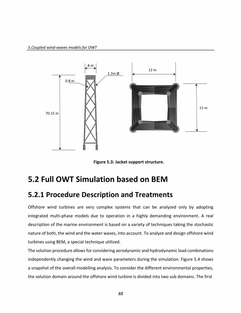
5.Coupled wind-waves models for OWT
88
5.2 Full OWT Simulation based on BEM
5.2.1 Procedure Description and Treatments
Offshore wind turbines are very complex systems that can be analyzed only by adopting
integrated multi-phase models due to operation in a highly demanding environment. A real
description of the marine environment is based on a variety of techniques taking the stochastic
nature of both, the wind and the water waves, into account. To analyze and design offshore wind
turbines using BEM, a special technique utilized.
The solution procedure allows for considering aerodynamic and hydrodynamic load combinations
independently changing the wind and wave parameters during the simulation. Figure 5.4 shows
a snapshot of the overall modelling analysis. To consider the different environmental properties,
the solution domain around the offshore wind turbine is divided into two sub domains. The first
12 m
12 m
70.15 m
0.8 m
Ø
8 m
1.2m Ø
Figure 5.3: Jacket support structure.

5.Coupled wind-waves models for OWT
89
Figure 5.4: OWT modelling in BEM code.
one covers the above free surface region and the second one below it. The coupled solvers
procedure in this code are capable of computing different environmental regions, where the first
solver will be responsible for the aerodynamic sub solution and the second one solves the
hydrodynamic sub domain. Each solver is a three-dimensional first-order panel method, as
described in chapter three. The body’s surfaces are discretized to quadrilateral panels, each panel
has a constant-strength singularity distribution of a source and a dipole and the boundary
conditions are satisfied at the control point. The governing equations are solved to calculate the
strength for each source and dipole.
Figure 5.5 shows the flowchart solution procedure, where two different subroutines (Global 1
and Global 2) are used to seek wind and hydro data required for the hydrodynamic and
aerodynamic simulators. In Global 1, the rotor operation conditions, wind velocity and the air
properties are considered. In Global 2, wave properties are included.
All offshore wind turbine loads are estimated at each iteration for the two parts, foundation part
and wind turbine. The wave potential is calculated using a hydrodynamics solver, where this
potential solver is capable of simulating regular and irregular waves.

5.Coupled wind-waves models for OWT
90
The generated wave potential 𝛷𝑤𝑎𝑣𝑒 is superimposed on the induced velocity potential of the
flow domain to find the local induced velocity potential on each foundation panels, as in Eq. (5.1):
Figure 5.5: Flowchart of BEM code procedure.
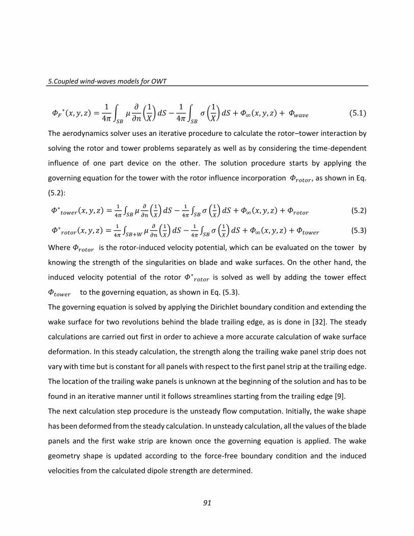
5.Coupled wind-waves models for OWT
91
𝛷𝐹∗(𝑥, 𝑦, 𝑧) =
1
4𝜋∫ 𝜇
𝜕
𝜕𝑛(1
𝑋)
𝑆𝐵
𝑑𝑆 −1
4𝜋∫ 𝜎 (
1
𝑋)
𝑆𝐵
𝑑𝑆 + 𝛷∞(𝑥, 𝑦, 𝑧) + 𝛷𝑤𝑎𝑣𝑒 (5.1)
The aerodynamics solver uses an iterative procedure to calculate the rotor–tower interaction by
solving the rotor and tower problems separately as well as by considering the time-dependent
influence of one part device on the other. The solution procedure starts by applying the
governing equation for the tower with the rotor influence incorporation 𝛷𝑟𝑜𝑡𝑜𝑟, as shown in Eq.
(5.2):
𝛷∗𝑡𝑜𝑤𝑒𝑟(𝑥, 𝑦, 𝑧) =1
4𝜋∫ 𝜇
𝜕
𝜕𝑛(1
𝑋)
𝑆𝐵𝑑𝑆 −
1
4𝜋∫ 𝜎 (
1
𝑋)
𝑆𝐵𝑑𝑆 + 𝛷∞(𝑥, 𝑦, 𝑧) + 𝛷𝑟𝑜𝑡𝑜𝑟 (5.2)
𝛷∗𝑟𝑜𝑡𝑜𝑟(𝑥, 𝑦, 𝑧) =1
4𝜋∫ 𝜇
𝜕
𝜕𝑛(1
𝑋)
𝑆𝐵+𝑊𝑑𝑆 −
1
4𝜋∫ 𝜎 (
1
𝑋)
𝑆𝐵𝑑𝑆 + 𝛷∞(𝑥, 𝑦, 𝑧) + 𝛷𝑡𝑜𝑤𝑒𝑟 (5.3)
Where 𝛷𝑟𝑜𝑡𝑜𝑟 is the rotor-induced velocity potential, which can be evaluated on the tower by
knowing the strength of the singularities on blade and wake surfaces. On the other hand, the
induced velocity potential of the rotor 𝛷∗𝑟𝑜𝑡𝑜𝑟 is solved as well by adding the tower effect
𝛷𝑡𝑜𝑤𝑒𝑟 to the governing equation, as shown in Eq. (5.3).
The governing equation is solved by applying the Dirichlet boundary condition and extending the
wake surface for two revolutions behind the blade trailing edge, as is done in [32]. The steady
calculations are carried out first in order to achieve a more accurate calculation of wake surface
deformation. In this steady calculation, the strength along the trailing wake panel strip does not
vary with time but is constant for all panels with respect to the first panel strip at the trailing edge.
The location of the trailing wake panels is unknown at the beginning of the solution and has to be
found in an iterative manner until it follows streamlines starting from the trailing edge [9].
The next calculation step procedure is the unsteady flow computation. Initially, the wake shape
has been deformed from the steady calculation. In unsteady calculation, all the values of the blade
panels and the first wake strip are known once the governing equation is applied. The wake
geometry shape is updated according to the force-free boundary condition and the induced
velocities from the calculated dipole strength are determined.

5.Coupled wind-waves models for OWT
92
Furthermore, split technique is applied in both solvers to handle the foundation part panels that
emerge out of the water on hydrodynamic solver and to solve wake-tower interaction on the
aerodynamic solver.
The split factor range is [0: 1]. If a split factor equals zero, the panel is located outside the
computation domain of the hydrodynamic solver, i.e. the strength singularity value is set at 0. If
a split factor equals 1, the panel is totally inside the computation domain; and between these two
values, the panel partly contributes to the solution and the influence of the panel on the solution
is reduced according to the valid split factor of the panel [32].
In the hydrodynamic solver, a split factor will be set to zero for the emerged parts of the
foundation body above the free surface, where it is calculated for every panel with respect to the
local wave elevation; this factor equals one for a panel which is totally inside the hydrodynamics
domain. To solve the wake-tower interaction in the aerodynamic solver, the split factor equals
zero for the wake panel that intersects or is near the tower body; and this value is equal to one
for other wake panels. The dipole strength excluded from the solution is saved and returned to
set again when these panels pass the tower region.
To simulate the flow around OWT in its natural environment, the inflow velocity distribution
should be considered as part of the velocity profile due to the wind shear action over the offshore
area. A new technique is implemented within the BEM code to contain the wind shear effect
profile, where the velocities upstream influence on the OWT body at different circumferential
positions and the velocity value at each point is dependent on its altitude, as shown in Figures 5.6
and 5.7. After applying the above solution procedure to the BEM code, the combined solvers are
capable of calculating the forces that effect on each part of the offshore wind turbine and of
determining the total main force (aerodynamic and hydrodynamic loads) for each iteration step
with a relatively short computing time and an adequate accuracy.

5.Coupled wind-waves models for OWT
93
Figure 5.6: Wind shear applying technique in BEM code.
Figure 5.7: Wind velocity distribution according to the log law.
5.Coupled wind-waves models for OWT
94
5.2.2 Panel Generation
Quadrate panel grids are generated on all model surfaces using in-house CAD code, and ANSYS
ICEM CFD is used for the panel generation of the tripod and jacket foundation parts due to their
complexity.
An OWT with a monopile foundation is discretized into 60x22 and 24x17 panels for the blade and
tower, respectively, and the monopile geometry is discretized into 19x13 panels using an in-house
CAD code, as shown in Figure 5.11-A.
A tripod foundation is used as the second OWT model, where an in-house CAD code is used for
the panel generation at the rotor and the tower with the same number of panels used in the
previous model. The grid generator ICEM CFD is utilized for generating the panels on the tripod
foundation part surfaces. The panels are generated using surface structural mesh type. The panels
have a quadrilateral shape. Figure 5.8-A shows panels around the body surfaces. The tripod
surface part is discretized using 1700 panels. The surface mesh procedure starts by defining multi
blocks on each body member. In order to better link the panels, the vertices of these blocks are
joined and refined at the connecting members, as shown in Figure 5.8-B.
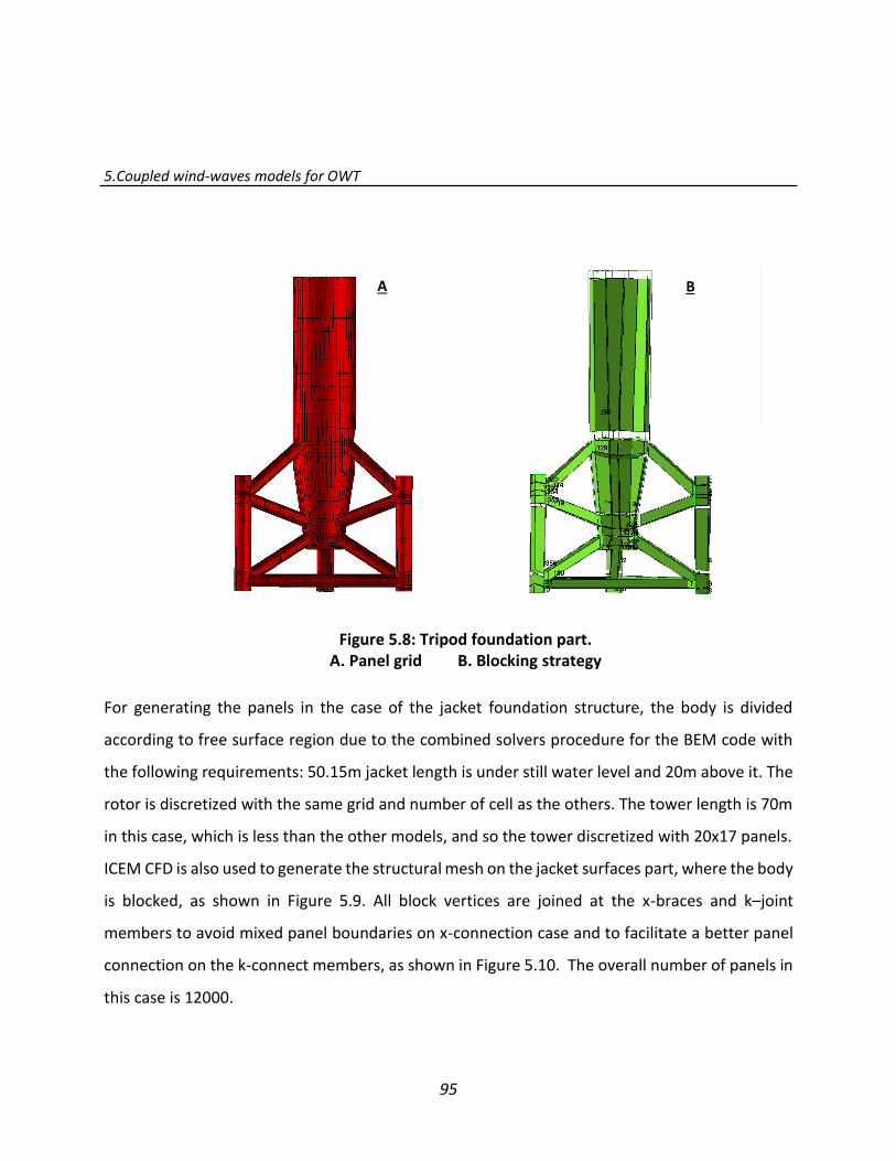
5.Coupled wind-waves models for OWT
95
For generating the panels in the case of the jacket foundation structure, the body is divided
according to free surface region due to the combined solvers procedure for the BEM code with
the following requirements: 50.15m jacket length is under still water level and 20m above it. The
rotor is discretized with the same grid and number of cell as the others. The tower length is 70m
in this case, which is less than the other models, and so the tower discretized with 20x17 panels.
ICEM CFD is also used to generate the structural mesh on the jacket surfaces part, where the body
is blocked, as shown in Figure 5.9. All block vertices are joined at the x-braces and k–joint
members to avoid mixed panel boundaries on x-connection case and to facilitate a better panel
connection on the k-connect members, as shown in Figure 5.10. The overall number of panels in
this case is 12000.
B A
Figure 5.8: Tripod foundation part. A. Panel grid B. Blocking strategy

5.Coupled wind-waves models for OWT
96
B A
A B
Figure 5.9: Jacket upper and lower parts. A. Panel grid B. Blocking strategy
Figure 5.10: Jacket x- braces and k-joint A. Panel grid B. Blocking strategy

5.Coupled wind-waves models for OWT
97
Monopile case Tripod case Jacket case
Blade 1300 1300 1300
Tower 450 450 350
Foundation 250 1700 12000
5.2.3 Initial and Boundary Conditions
The BEM simulations are conducted using the combined solvers procedure, where each solver
has an input subroutine: Global 1 for the aerodynamic solver and Global 2 for the hydrodynamic
solver. Global 1 contains blade and tower grids and the inflow wind velocity is chosen according
to wind shear principle over offshore area, where the inflow wind velocity changes in respect to
height according to the log law wind profile shown in Figure 5.7.
Table 5.1: Panel grids number in OWT cases.
Figure 5.11: OWT panel grids.
A. Monopile B. Tripod C. Jacket
A B C

5.Coupled wind-waves models for OWT
98
Table 5.2: Waves properties.
The rotor angular velocity is 1.267 rad/sec, the wake length is extended for two revolutions from
the blade trailing edge and a time-increment is chosen so that the rotor blades advance 5o for
each iteration. Global 2 subroutine contains foundation grids and wave properties, where the
wave properties are 2m wave amplitude, 7.16 sec wave period and the water depth for the three
cases is (15m, 24m, 50m), respectively.
𝑯 𝝀 𝒅 𝒅 𝝀⁄ 𝑷𝒆𝒓𝒊𝒐𝒅 𝑯 𝒅⁄ 𝑯 𝝀⁄ Monopile case 4 69.9 15 0.214 7.16 0.266667 0.057
Tripod case 4 76.9 24 0.312 7.16 0.166667 0.052
Jacket case 4 80 50 0.625 7.16 0.08 0.05
According to (𝑑/𝜆) ratio, the wave kinematics can be calculated. For monopile and tripod cases,
the waves are generated in intermediate water (water depth is shorter than half the wave length)
and both water depth and wave length have a significant influence on the wave kinematics
computation. The waves in the jacket case are generated in deep water, meaning there are no
effects from sea bed on the wave kinematics. Each wave’s properties are shown in Table 5.2,
where the wave’s period is the same for all cases and the wave’s steepness are below the breaking
criteria. The time step in each solver is 0.07sec. Both solvers simulate whole OWT parts as a lifting
body, where a constant dipole and source are located at each panel’s collection point. The
governing equation is solved with the setting boundary condition to calculate the induced velocity
at each panel and to determine the pressure and force values, which are presented in the next
section.
5.3 Full OWT Simulation based on RANSE
5.3.1 Domain and Meshing The same geometrical configurations are used in this calculation as in the previous BEM code
simulations. The computational domains are shown in Figure 5.12-A. Each domain contains a
stationary and rotational region domain. A cylindrical rotating domain is created around the hub

5.Coupled wind-waves models for OWT
99
and the blades and has the same rotor rotating speed. The stationary region domain contains all
other OWT parts. Interfaces are required to connect unmatched meshes within the two region
domains. ICEM CFD is used for mesh generation at all domains using unstructured mesh.
Unstructured mesh offers more possibilities to generate an adaptive mesh which fits better to
the complex body surface. The mesh on the blade surfaces is generated with the same mesh size
as is used in the previous chapter. The surface mesh type is a triangle with 0.4m2 area generated
with a low deviation value for better mesh deformation around the surfaces. The three interface
surfaces have the same mesh area of 1m2.
Surfaces Mesh setting
Blade 0.4 m2 with 0.01 deviation factor
Nacelle, tower 0.5 m2
Foundation 0.35 m2
Inlet, outlet, sides, top, bottom 8 m2
Interfaces surfaces 1 m2
Max. fluid cell size 10 m3
Free surface cell size 1.15 m3
In order to capture the wave characteristics with a high degree of accuracy, the volume mesh is
generated in conjunction with the surface mesh using a tetrahedral shape element. The free
surface region is specified as a high density region compared to other domain parts, as shown in
Figure 5.12-B, which is extended to ±5 𝑚 above and below still water level. Free surface mesh
size setting correlates to the wave properties, where the cell number should be more than 10
elements per wave height and 111 elements per wave length [89], so cell volume in this region is
1.15m3. In order to adequately resolve the viscous sub layer near the wall, prism layers are applied
to the boundary wall surface, where the initial cell thickness is 2mm, the expansion ratio is
approximately 1.2, and the number of layers is 20, as shown in Figure 5.13. Here, the boundary
layer deforms around the blade surface. The initial setting and the refinement on both free
surface and around blade region lead to a final mesh number as shown in Table 5.4.
Table 5.3: Mesh generation setting.

5.Coupled wind-waves models for OWT
100
Monopile case Length = 3𝐷𝑖𝑅
Height=1.8𝐷𝑖𝑅
Width =2.5𝐷𝑖𝑅
A B
Tripod case
Length = 3𝐷𝑖𝑅
Height=2𝐷𝑖𝑅
Width =2.5𝐷𝑖𝑅
Jacket case
Length = 3𝐷𝑖𝑅
Height=2. 2𝐷𝑖𝑅
Width =2.5𝐷𝑖𝑅
Figure 5.12: OWT models. A. Domain dimensions B. Mesh domain

5.Coupled wind-waves models for OWT
101
.
Model type foundation Total node number Total mesh cell number
OWT with Monopile 7254909 22.830 Million
OWT with Tripod 7608842 28.148 Million
OWT with Jacket 8287603 35.257 Million
5.3.2 Initial and Boundary Conditions
In the three simulation cases, the same definition of the boundary conditions as well as the initial
conditions are applied. Wall with no slip boundary condition is applied for all OWT parts in all
cases as well as the sea bed. The solution domain consists of two homogeneous fluids with an
interface compression level of 2; these fluids are water and air, and the density and viscosity used
is given in Table 5.5. The SST turbulent model is used in all cases. Isothermal heat transfer and
buoyancy are used and the buoyancy reference density is set equal to air density.
Table 5.4: Number of mesh in different OWT cases.
Figure 5.13: Blade surface mesh and boundary layers.

5.Coupled wind-waves models for OWT
102
The free surface is modeled using a homogeneous, coupled volume of fluid (VOF) approach which
is developed in [36], where air and water share a common flow field. Each fluid has a volume
fraction and the free surface is tracked by finding the evolution of the variable on each cell in
every time step.
An expression formula is used to specify the air velocity at inlet boundary condition using the
wind shear profile over offshore area presented in chapter two. Figure 5.14 shows velocity profile
wind against altitude. The wind velocity at hub height is 8.7m/sec and 7.7m/sec at the lowest
position of the blade tip, while it is 9.7m/sec at the highest position, leading to a velocity
difference of about 20%. The forces scale with velocity squared, hence the forces increase from
rotor bottom to the top by approximately 36%.
Water velocity is defined at the inlet region to generate progressive regular two-dimensional
wave acting at the body. The wave velocity is based upon Airy’s linear wave theory and have two
components in both horizontal and vertical directions:
𝑢 = (𝑢𝑤𝑎𝑣𝑒 ∗ 𝛿𝑤𝑎𝑡𝑒𝑟) + (𝑢𝑤𝑖𝑛𝑑 ∗ 𝛿𝑎𝑖𝑟) 𝑣 = 0 𝑤 = (𝑤𝑤𝑎𝑣𝑒 ∗ 𝛿𝑤𝑎𝑡𝑒𝑟)
Fluid Density [kg/m3] Dynamic viscosity [kg/m.sec]
Water 1025 8.899 10-4
Air 1.185 1. 831 10-5
Table 5.5: Fluid specification.

5.Coupled wind-waves models for OWT
103
The outlet region is defined relative to static pressure, allowing the pressure profile at the outlet
to vary according to upstream influences while limiting the average pressure to the total pressure,
which is defined to contain conditions of hydrostatic pressure and wave dynamic pressure.
Opening boundary condition is chosen for the top region and symmetry boundary condition is
chosen for the sides of numerical wave tank. 2nd-order Backward Euler Scheme is used and the
number of loops is set to 1 to 10 loops in each time step.
The wave properties and the rotor angular velocity are considered to be the same as in the BEM
code setting, which allows for comparing the results. In order to solve the unsteady problem, the
Figure 5.14: Log-law wind profile.
𝑣𝑧

5.Coupled wind-waves models for OWT
104
initial condition is specified for both domains. The velocity is considered in Cartesian coordinates
with the same velocity component expression used in the inlet boundary condition. Furthermore,
the pressure value is initialized according to the combination of the hydrostatic pressure and
wave dynamic pressure. With a given wave property at the initial time, the convergence will be
improved.
5.4 Results
In OWT design, the prediction of extreme loads are associated with a target including a complete
integration of all available loads data. Many traditional approaches for estimating the ultimate
capacity of OWT are not ideally suited to an analysis of OWT under wave and wind combination.
Coupled aerodynamic and hydrodynamic loads are investigated in this study using two different
methods, as mentioned above. The described methods are applied to calculate the environmental
loads effects on three different OWT configurations, which are assumed to be fully fixed at the
mudline under similar wind and wave characteristics.
For studying environmental impact, wave model influence is investigated with the two solver
solutions. Figure 5.15 shows the wave elevation and velocity components at a specified point on
the free surface logged as a function of time during the analysis for the three cases. This study
point is 10m upstream from the OWT body, where the water wave at this point is considered to
be unaffected by the foundation body or, in other words, wave kinematics is analyzed before the
waves hit the OWT foundation.
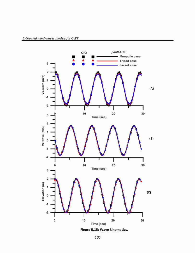
5.Coupled wind-waves models for OWT
105
Figure 5.15: Wave kinematics.
(C)
(A)
(B)

5.Coupled wind-waves models for OWT
106
In figure 5.15-A and B the horizontal and vertical water velocity components in the three cases
are compared for the two solvers during 30sec, which is about 4.2 wave period cycles. As is
expected, high wave steepness and decreased water depths lead to high velocity components.
Therefore, the highest velocity takes place for the monopile case and the lowest for the jacket
case. This difference is clearer at the horizontal velocity component than the vertical component
because of the point’s location on the free surface (Z=0). Figure 5.15-C shows the surface
elevation at this point compared between the two results for all the cases.
It can be seen that a good agreement is obtained for the horizontal and vertical velocity
components as well as the wave’s elevation values, which indicates that the boundary condition
and solver settings are correct.
As expected, a reduction of the wave amplitude takes place near the outlet of the RANS
simulation domain because of the energy losses on the structure walls and sea bed. In the BEM
solution, the damping of the wave amplitude is negligible as no friction losses on sea bed or on
structure components can be considered in the simulation.
To give a comprehensive overview for all the simulations, Figures 5.16, 5.17, and 5.18 provide the
pressure coefficient distribution for all OWT results obtained from the two applied solvers. A part
from this, the wake structure extends to two revolutions behind the wind turbine rotor in the
BEM code results. The pressure coefficient is calculated in the aerodynamic field based on the
maximum field velocity located at the blade tip; and in the hydrodynamic field based on the
particle velocity at the wave crest. The free surface elevation for the monopile case is shown in
Figure 5.16, where the wave crest is just in front of the monopile body. The free surface color is
used to visualize the horizontal wave velocity component in Figure 5.17 (tripod case); obviously,
maximum velocity value hits the tripod body. The free surface color in Figure 5.18 indicates the
vertical wave velocity component in the jacket case.
5.Coupled wind-waves models for OWT
107
Figures 5.19, 5.20, and 5.21 present the pressure coefficient distribution on the surfaces of the
foundation parts for the three cases surfaces due to wave dynamic pressure. Since the wave is
proceeding, particles under the crest are accelerating downward, so the maximum pressure is
attained directly below the wave crest. While the reverse is true under the wave trough, where
the minimum of the pressure is attained. Between the crest and trough, the acceleration is
horizontal, so the vertical pressure distribution is hydrostatic [29]. In deep water, the dynamic
part of the pressure undergoes an exponential decay at distances below the still water line, so
that the dynamic pressure is small below one-half wavelength in depth, as in the jacket case. The
integration of the dynamic pressure load influence over the body surface delivers the incident
wave force.
To determine the quantitative differences that can arise when using different calculation
methods, all the inflow OWT model loads are made in dimensionless form by using the mean
value for the last three amplitude loads obtained from BEM code, as shown in Table 5.6. Inflow
direction loads are higher compared to top and side force components [103]. This approach is a
useful and powerful comparison tool to grasp the loading contribution details for each OWT parts
at total devise force.
Figures 5.22, 5.23 and 5.24 show the time history of the thrust contribution value obtained from
the two solvers for the three cases. The blade rotor experiences the same thrust value in all cases
due to the same geometry and operation condition. The RANSE solver predicts a thrust average
value of 609.8 kN, and 567 kN for the BEM code. The differences in the mean magnitude of rotor
thrust is about 8%. The results show acceptable agreement with both methods. According to the
operation condition and the airfoil blade, the flow is attached and no stall condition on the rotor
blade, which is also seen for the flow simulation around blades at chapter four. In this chapter,
the log-law wind effect is utilized instead of using uniform velocity, which have no large effects
on general flow trends [105].
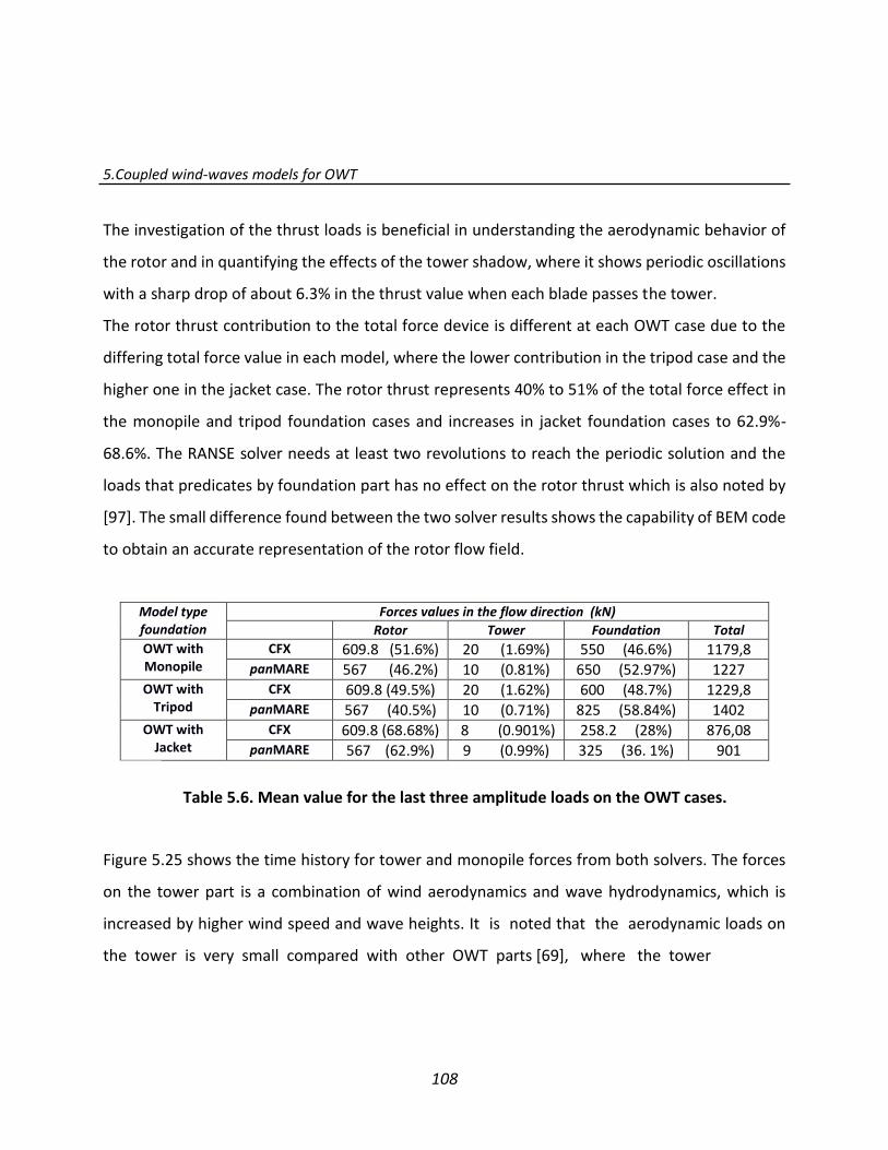
5.Coupled wind-waves models for OWT
108
The investigation of the thrust loads is beneficial in understanding the aerodynamic behavior of
the rotor and in quantifying the effects of the tower shadow, where it shows periodic oscillations
with a sharp drop of about 6.3% in the thrust value when each blade passes the tower.
The rotor thrust contribution to the total force device is different at each OWT case due to the
differing total force value in each model, where the lower contribution in the tripod case and the
higher one in the jacket case. The rotor thrust represents 40% to 51% of the total force effect in
the monopile and tripod foundation cases and increases in jacket foundation cases to 62.9%-
68.6%. The RANSE solver needs at least two revolutions to reach the periodic solution and the
loads that predicates by foundation part has no effect on the rotor thrust which is also noted by
[97]. The small difference found between the two solver results shows the capability of BEM code
to obtain an accurate representation of the rotor flow field.
Model type foundation
Forces values in the flow direction (kN)
Rotor Tower Foundation Total
OWT with Monopile
CFX 609.8 (51.6%) 20 (1.69%) 550 (46.6%) 1179,8 panMARE 567 (46.2%) 10 (0.81%) 650 (52.97%) 1227
OWT with Tripod
CFX 609.8 (49.5%) 20 (1.62%) 600 (48.7%) 1229,8 panMARE 567 (40.5%) 10 (0.71%) 825 (58.84%) 1402
OWT with Jacket
CFX 609.8 (68.68%) 8 (0.901%) 258.2 (28%) 876,08 panMARE 567 (62.9%) 9 (0.99%) 325 (36. 1%) 901
Figure 5.25 shows the time history for tower and monopile forces from both solvers. The forces
on the tower part is a combination of wind aerodynamics and wave hydrodynamics, which is
increased by higher wind speed and wave heights. It is noted that the aerodynamic loads on
the tower is very small compared with other OWT parts [69], where the tower
Table 5.6. Mean value for the last three amplitude loads on the OWT cases.
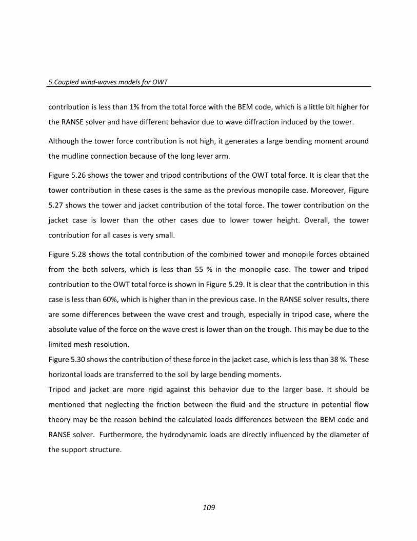
5.Coupled wind-waves models for OWT
109
contribution is less than 1% from the total force with the BEM code, which is a little bit higher for
the RANSE solver and have different behavior due to wave diffraction induced by the tower.
Although the tower force contribution is not high, it generates a large bending moment around
the mudline connection because of the long lever arm.
Figure 5.26 shows the tower and tripod contributions of the OWT total force. It is clear that the
tower contribution in these cases is the same as the previous monopile case. Moreover, Figure
5.27 shows the tower and jacket contribution of the total force. The tower contribution on the
jacket case is lower than the other cases due to lower tower height. Overall, the tower
contribution for all cases is very small.
Figure 5.28 shows the total contribution of the combined tower and monopile forces obtained
from the both solvers, which is less than 55 % in the monopile case. The tower and tripod
contribution to the OWT total force is shown in Figure 5.29. It is clear that the contribution in this
case is less than 60%, which is higher than in the previous case. In the RANSE solver results, there
are some differences between the wave crest and trough, especially in tripod case, where the
absolute value of the force on the wave crest is lower than on the trough. This may be due to the
limited mesh resolution.
Figure 5.30 shows the contribution of these force in the jacket case, which is less than 38 %. These
horizontal loads are transferred to the soil by large bending moments.
Tripod and jacket are more rigid against this behavior due to the larger base. It should be
mentioned that neglecting the friction between the fluid and the structure in potential flow
theory may be the reason behind the calculated loads differences between the BEM code and
RANSE solver. Furthermore, the hydrodynamic loads are directly influenced by the diameter of
the support structure.

5.Coupled wind-waves models for OWT
110
A foundation structure with a small diameter, such as a jacket structures, is generally drag
dominated. But at larger diameters, monopile and tripod are large enough to incur both inertia
and drag loads, meaning that jacket force is lower than other models. Also tripod and jacket cases
have multiple small element which have less influence on the flow field wave progress.
Finally, Figure 5.31 shows the total force on the monopile OWT that results from both simulations;
and Figures 5.32 and 5.33 show the total force on the tripod and jacket OWTs, respectively. It is
clear that the RANSE solver must complete three wave periods (21 sec) before getting periodic
solution results.
As can be seen from the above results, the rotor and foundation parts have the largest
contribution of the total force. Although the structural theory for the two codes is completely
different, it appears the OWT flow in all cases have been successfully represented.
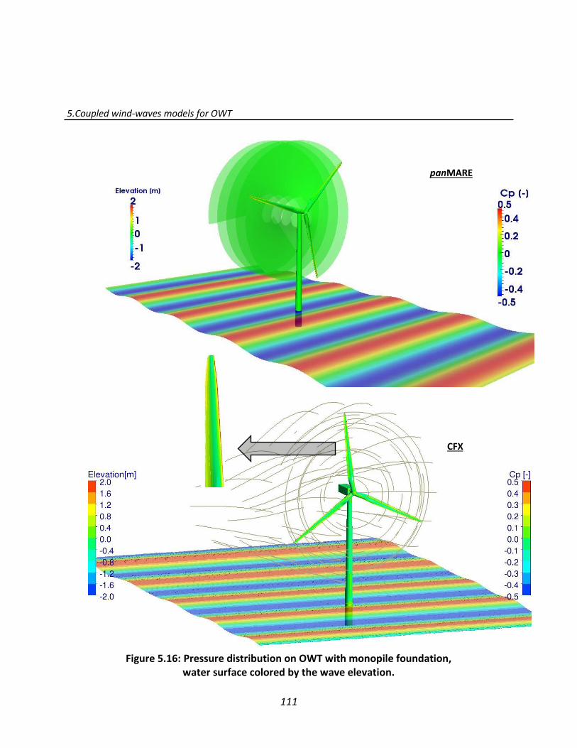
5.Coupled wind-waves models for OWT
111
Figure 5.16: Pressure distribution on OWT with monopile foundation, water surface colored by the wave elevation.
CFX
panMARE
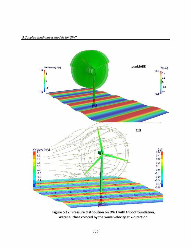
5.Coupled wind-waves models for OWT
112
CFX
Figure 5.17: Pressure distribution on OWT with tripod foundation,
water surface colored by the wave velocity at x-direction.
panMARE
5.Coupled wind-waves models for OWT
113
Figure 5.18: Pressure distribution on OWT with jacket foundation, water surface colored by the wave velocity at z-direction.
panMARE
CFX

5.Coupled wind-waves models for OWT
114
Figure 5.19: Pressure distribution on monopile foundation.
panMARE
CFX
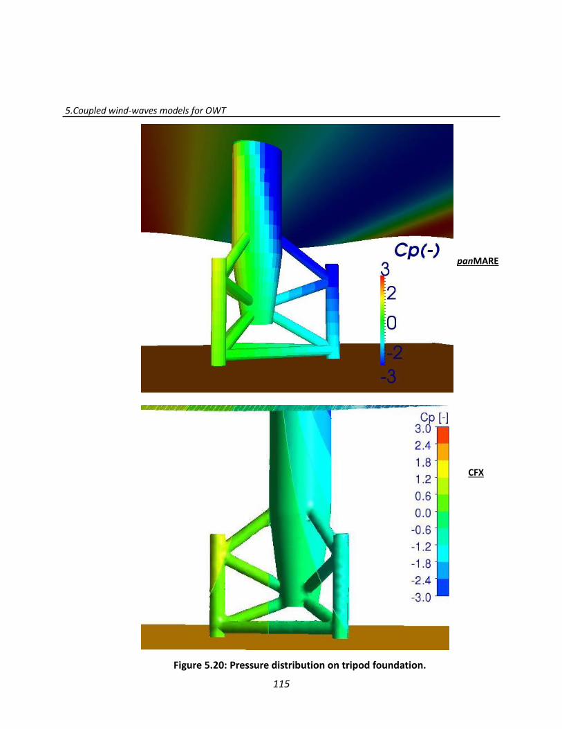
5.Coupled wind-waves models for OWT
115
CFX
Figure 5.20: Pressure distribution on tripod foundation.
panMARE
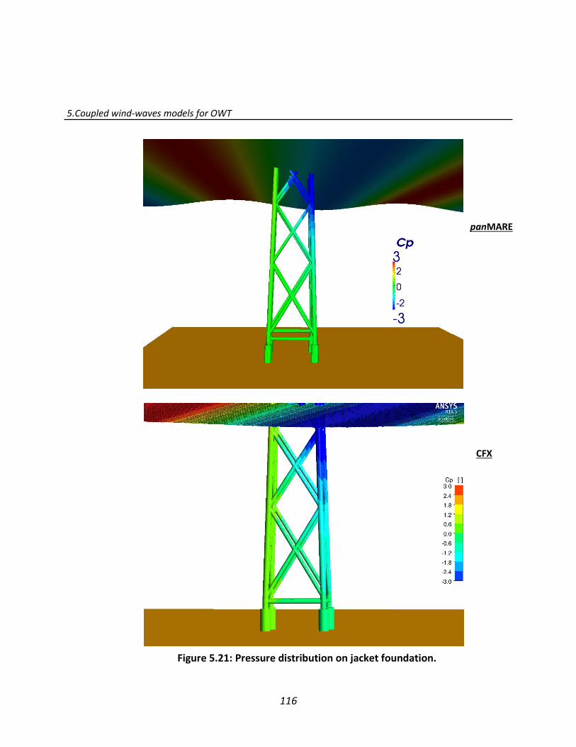
5.Coupled wind-waves models for OWT
116
panMARE
CFX
Figure 5.21: Pressure distribution on jacket foundation.
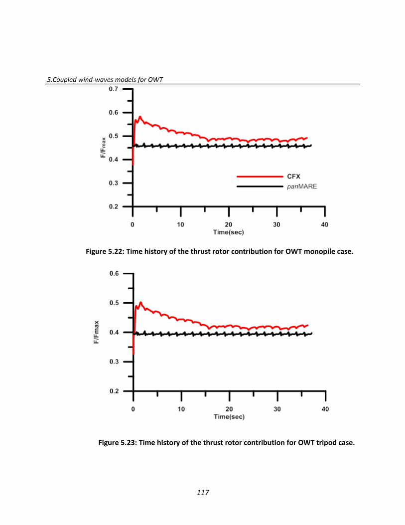
5.Coupled wind-waves models for OWT
117
Figure 5.22: Time history of the thrust rotor contribution for OWT monopile case.
Figure 5.23: Time history of the thrust rotor contribution for OWT tripod case.
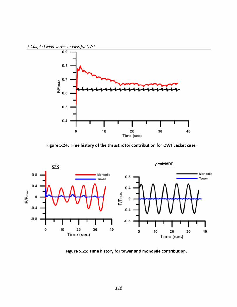
5.Coupled wind-waves models for OWT
118
Figure 5.24: Time history of the thrust rotor contribution for OWT Jacket case.
Figure 5.25: Time history for tower and monopile contribution.
CFX panMARE
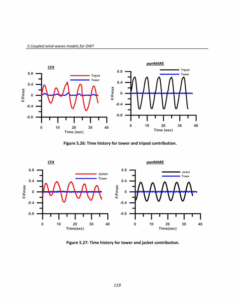
5.Coupled wind-waves models for OWT
119
CFX panMARE
CFX panMARE
Figure 5.27: Time history for tower and jacket contribution.
Figure 5.26: Time history for tower and tripod contribution.

5.Coupled wind-waves models for OWT
120
Figure 5.28: Time history for the tower and monopile contribution for OWT monopile case.
Figure 5.29: Time history for the tower and tripod contribution for OWT tripod case.
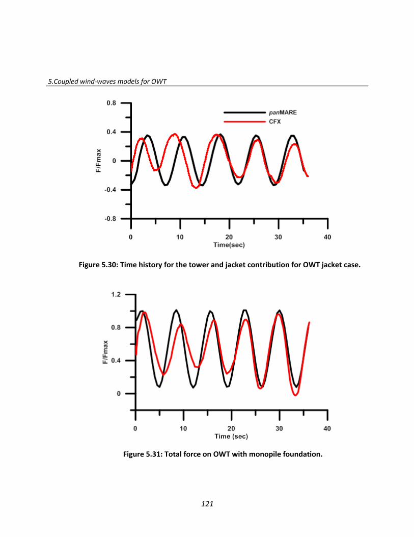
5.Coupled wind-waves models for OWT
121
Figure 5.30: Time history for the tower and jacket contribution for OWT jacket case.
Figure 5.31: Total force on OWT with monopile foundation.
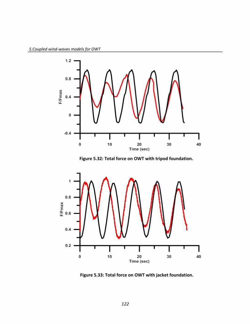
5.Coupled wind-waves models for OWT
122
Figure 5.32: Total force on OWT with tripod foundation.
Figure 5.33: Total force on OWT with jacket foundation.
123
Conclusions and Future Work
A high fidelity approach for coupling aerodynamic and hydrodynamics loads on an OWT using
BEM code is presented. All the results obtained from the BEM code are compared with results
obtained from ANSYS CFX. The applied BEM code is a first-order panel method based on potential
theory and the flow is assumed to be incompressible, irrotational and inviscid. ANSYS CFX is based
on solving full RANS equations combined with SST turbulence model. Both approaches have the
potential for simulating onshore and offshore wind turbines under different operational
conditions, including uniform wind speed as well as atmospheric wind shear.
Initially, rotor only and rotor with tower are simulated using these different solvers under the
same operation conditions, which are 11.4 m/s uniform wind speed and 1.267 rad/sec rotational
speed. The BEM code solution procedure starts with body surface discretization, where the in-
house CAD code is used to discretize the rotor geometry using 3600 panels, and 4050 panels for
both rotor and tower geometry in the other cases.
Grid generation is an important preprocessing step in the simulation of the previous cases using
RANS solver. The two cases are discretized using ICEM CFD with 10.2 and 11.3 million cells. For
analyzing the results obtained from the two codes, pressure distributions on the blade surfaces
are compared. A good agreement is achieved on blade pressure side but some small differences
can be seen on the blade suction side, especially near the leading edge area. Furthermore, blade-
tower interaction effects have been detected, where a pressure drop occurs on both the blade
and tower for every blade passing the tower.
6.Conclusions and future works
124
For analyzing and validating the hydrodynamic loads results for the both solvers, the flow on a
slender cylinder in regular wave effects is investigated. This case is discretized into 2400 panels
using the in-house CAD code, and 7.2 million cells using ICEM CFD, and the wave properties are
15m wave length and 0.5m wave height.
This case is important to verify the solver settings, especially for the hydrodynamic OWT part.
Therefore, the time history of the cylinder hydrodynamic forces at inflow direction obtained from
the solvers are compared with forces obtained from the Morison equation. The comparison
confirms the ability of both codes to calculate the hydrodynamic loads with an acceptable
accuracy.
The next part of the study focuses on simulating an offshore wind turbine with the combination
of wind and wave loads using the same two solvers. OWT is a complicated case due to different
environmental impacts. The solution procedure using BEM code involves a combinations of two
solvers: the first solver for simulating OWT parts above still water level and the second for below.
The flow on OWT is also simulated using RANS solver, where the free surface is modeled using a
homogeneous coupled volume of fluid approach.
Three different OWT configurations are investigated, which consist of a generic 5MW NREL rotor
with three different foundations types: monopile, tripod and jacket. These three configurations
are analyzed using the two solvers under the effect of atmospheric wind shear and a rotor
rotation of 1.267 rad/sec. The wave properties are 7.16 sec wave period, 4m wave height and the
water depth for the three cases is (15m, 24m, 50m) respectively.
The comparison of the results from the two codes starts with the environmental part, where the
calculated wave kinematics at a specified point on the free surface are compared and a good
agreement is achieved. The force is calculated at each OWT part to arrive at the total force. The
time history of the forces at each OWT part at inflow direction are presented in a dimensionless

6.Conclusions and future works
125
form with respect to the mean value for the last three amplitude loads obtained from the BEM
code. This approach is more convenient to capture the OWT parts loading contribution details.
The relative rotor load contributions are different in each OWT case, where the rotor contribution
is lower in the tripod case and higher in the jacket case.
The relative rotor loads represent from 40% to 51% of the total force in the monopile and tripod
cases and increases in the jacket case to 62.9%-68.6%. An acceptable difference is found between
the two solvers for the rotor loads calculation, which is about (8%). These results confirm the
capability of the panMARE code to characterize the temporal and spatial natures of the flow near
the rotor. Moreover, the time history for the tower and foundation forces contribution are
compared for each configuration. Although the tower contribution is quite small with less than
1.7% of the maximum obtained force, it generates a large bending moment around the mudline
connection because of the long arm.
The relative contribution of the tower and foundation loads obtained from the both solvers is less
than 55% from the total load in monopile case, which increases to 60% for tripod case and
decreases to 38% in the jacket case. The calculated hydrodynamic loads on the jacket foundation
type is lower than the loads in the other two cases because of the smaller diameter of the jacket
foundation. These results emphasize the fact that the effect of the hydrodynamic cycle load is
the most important contribution to the main load effects.
This work can be extended by adding the current effects to the 2D regular wave on the calculation
of hydrodynamic loads. The reason for using the 2D wave in this study is to have the same basis
for the comparison between the two codes. Further, other wave models can be simulated using a
combination of different regular waves which collectively result in a spectrum as well as to consider
the diffraction and reflection in the computations for the monopile. The numerical methods can be
developed for simulating
6.Conclusions and future works
126
the dynamic behaviour of floating offshore wind turbines, where a variety of parameters are
influencing the motion behaviour of the floating platform and its position. In this case, an additional
requirement for the solvers coupling is necessary to estimate the time dependent acting forces.
Furthermore, the calculation of the aerodynamic loads can be improved by adding corrections to
take into account the influence of turbulent and separation effects.

127
Bibliography
[1] Anderson, J. D. Computational Fluid Dynamics: The Basics with Application. 1995.
[2] Abedi, H., Lars, D. and Spyros, V. Vortex method application for aerodynamic loads on rotor
blades. EWEA 2013: Europe’s Premier Wind Energy Event, Vienna, 4-7 February 2013.
[3] Agarwal, P. and Manuel, L. Simulation of offshore wind turbine response for long-term extreme
load prediction. Journal of Engineering Structures, 31, pp. 2236-2246, 2009.
[4] American Bureau of Shipping Corporate Offshore Technology, Renewables., Design Standards for
Offshore Wind Farms. U.S. Department of the Interior Bureau of Ocean Energy Management,
Regulation, and Enforcement, September 2011.
[5] Au, M.C. and Brebbia, C.A. Diffraction of water waves for vertical cylinders using boundary
elements. Appl. Math. Modelling Vol. 7, pp.106-114, 1983.
[6] ANSYS CFX-Solver theory guide, November 2013.
[7] Bazilevs, Y., Hsu, M., Akkerman, I., Wright, S., Takizawa, K., Henicke, B., Spielman, T. and Tezduyar,
T. E. 3D Simulation of wind turbine rotors at full scale. part I: geometry modelling and
aerodynamics. International Journal for Numerical Methods in Fluids 65 (1-3): 207–235.
doi:10.1002/fld.2400, 2010.
[8] Bazilevs, Y. and Hsu, M. Fluid–structure interaction modelling of wind turbines: simulating the full
machine. Springer-Verlag, Comput. Mech. 50,821–833, 2012.
[9] Bauer, M. and Abdel-Maksoud, M. Propeller induced loads on quay walls . 2nd Workshop on Ports
for Container Ships of Future Generations, Publications of the Institute of Geotechnics and
Construction Management of Hamburg University of Technology, Vol. 22, Germany, February
2011.
[10] Burton, T., Sharpe, D., Jenkins, N. and Bossanyi, E. Wind energy handbook .JohnWiley & Sons,
2001.
[11] Bermudez, L., Velazquez, A. and Matesanz, A. Numerical simulation of unsteady aerodynamics
effects in horizontal-axis wind turbines. Solar Energy 68, 1, 9-21, 2000.

Bibliography
128
[12] Blasques, J.P. and Natarajan, A. Mean load effects on the fatigue life of offshore wind turbine
monopile foundations. V International Conference on Computational Methods in Marine
Engineering, 2013.
[13] Benjanirat, S. Computational studies of horizontal axis wind turbines in highwind speed
condition using advanced turbulence models. Ph.D. thesis, Georgia Institute of Technology,
December 2006.
[14] Ceyhan, Ö. Aerodynamic design and optimization of horizontal axis wind turbines by using BEM
theory and genetic algorithm. M.Sc. thesis, Aerospace Engineering Department, Middle East
Technical University, Ankara, Turkey, 2008.
[15] Chakrabarti, S.K. Hydrodynamic of offshore structures. Springer-Verlag Berlin, Heidelberg
1978.
[16] Choi, N., Nam, S. H., Jong, J. H. and Kim, K. C. Numerical study on the horizontal axis turbines
arrangement in a wind farm: Effect of separation distance on the turbine aerodynamic power
output. WindEng.Ind.Aerodyn.117, 2013.
[17] Chakrabarti, S. K., Barnett, J., Kanchi, H., Mehta, A. and Yim, J. Design analysis of a truss
pontoon semi-submersible concept in deep water. Ocean Engineering, Vol. 34, pp. 621-629,
2007.
[18] Carrel, V. Development of a Wind Turbine Rotor Flow Panel Method. Energy research of the
Netherland, 2011.
[19] Dumitresch, H. and Cardos, V. Wind Turbine Aerodynamic Performance by Lifting Line Method.
International Journal of Rotating Machinery, 1998, Vol. 4, No. 3, pp. 141-149.
[20] Damgaard, Ch. E., Lars, Y., Helge, G., Erik, A. H., Johansen, T. and Mathilde, L. D. Wave load s on
offshore wind turbine foundations in shallow water. Proceedings of the European Offshore Wind
Conference, The European Wind Energy Association, 2007.
[21] Der Tempel, J. V. Design of Support Structures for Offshore Wind Turbines. Ph.D. thesis,
university of Delft, 2006.
[22] Derakhshan, S. and Tavaziani, A. Study of Wind Turbine Aerodynamic Performance Using
Numerical Methods. Journal of Clean Energy Technologies, Vol. 3, No. 2, March 2015.
[23] Duncan, J. H. The breaking and non-breaking wave resistance of a two-dimensional hydrofoil.
Journal of Fluid Mechanics, 126:507-520, 1983.
[24] Erich, H. Wind Turbines Fundamentals, Technologies, Application, Economics. Third translated
edition, Springer-Verlag Berlin Heidelberg, 2013.
Bibliography
129
[25]
Elfarra, M. A. Horizontal axis wind turbine rotor blade: winglet and twist aerodynamic design
and optimization using CFD. Ph.D. Thesis, Aerospace Engineering Department, Middle East
Technical University, 2011.
[26] Fernández, Z. Offshore wind energy. M.Sc. theses, Technical aspects and feasibility study of
offshore on Spanish coasts, Spanish, 2010.
[27]
Ferreira, G. D., Lemmerhirt, M., König, M., Abdel-Maksoud, M. and Düster, A. Numerical and
experimental investigation regarding the landing manoeuvre of a catamaran vessel at an
offshore wind turbine in waves. Proceedings of the ASME 2015 34th International Conference on
Ocean, Offshore and Arctic Engineering OMAE 2015 , St. John’s, Newfoundland, Canada ,May
31-June 5, 2015.
[28] Frigaard, P., Hansen, E., Christensen, E. and Jensen, M. Effect of breaking waves on scour
processes around circular offshore wind turbine foundations. Copenhagen Offshore Wind 2005
Conference, Copenhagen, Denmark, 2005.
[29] Faltinsen, O. M. Sea Loads on Ships and Offshore Structures. Cambridge University Press, UK,
1995.
[30] Fabian, V., Wojciech, P. and Kaufer, D. Description of a Basic Model of the "UpWind Reference
Jacket" for Code Comparison in the OC4 Project under IEA Wind Annex 30. Technical Report,
Fraunhofer Institute for Wind Energy and Energy System Technology IWES, 2011.
[31] Gebhardt, C.G., Preidikman, S. and Massa, J.C. Numerical simulations of the aerodynamic
behaviour of large horizontal-axis wind turbines. International Journal of Hydrogen Energy,
2010.
[32] Greve, M. Non-viscous calculation of propeller forces under consideration of free surface effects.
Ph.D. theses, Fluid Dynamic and Ship Theory Institute, Hamburg university of technology, 2015.
[33] Hsu, M., Akkerman, I. and Bazilevs, Y. Finite Element Simulation of Wind Turbine Aerodynamics:
Validation Study Using NREL Phase VI Experiment. Wind Energy. doi:10.1002/we.1599, 2013.
[34] Haas, P. Numerical simulation of nonlinear water wave using a panel method. Domain
decomposition and applications. Ph.D. thesis, Twente University, 1997.
[35] Horia, D. and Vldimir, C. Wind Turbine Aerodynamic Performance by Lifting Line Method.
International Journal of Rotating Machinery, Vol. 4, No. 3, pp. 141-149,1998.

Bibliography
130
[36] Hirt, C. W. and Nichols, B. D. Volume of fluid (VOF) method for the dynamics of free boundaries.
Journal of Computational Physics, 39:201-225, 1981.
[37] Henderson, A.R. and Zaaijer M.B. Hydrodynamic loading on offshore wind turbines. ISOPE Conference, Toulon, France, 23-28 May 2004.
[38] Ingram, G. Wind Turbine Blade Analysis using the Blade Element Momentum Method.
https://community.dur.ac.uk/g.l.ingram/download/wind_turbine_design.pdf, Durham
University, 2011.
[39] Iijima, K., Kim J. and Fujikubo, M. Coupled aerodynamic and hydro elastic analysis of an offshore
floating wind turbine system under wind and wave loads. Proc. 29th , Intl. Conf. on Ocean,
Offshore and Arctic Eng., OMAE-20772,2010.
[40] Jimenez, A., Crespo, A., Migoya, E. and Garcia, J. Large-eddy simulation of spectral coherence in
a wind turbine wake. IOP Publishing Ltd, 2008.
[41] Jonkman, B. J. TurbSim user’s guide: Version 1.50. Report No. NREL/TP-500-46198, National
Renewable Energy Laboratory, 2009.
[42] Jose prasobh, M. J., Karmakar, D. and Satheesh babu, P. K. Coupled dynamic analysis of spar-
type offshore floating wind turbine. International Conference on Emerging Trends in
Engineering and Management (ICETEM14) 30 -31, December, Ernakulam, India, 2014.
[43] Jonkman, J. M. and Buhl Jr, M. L. FAST User’s Guide. Technical Report NREL/EL-500-29798.
Golden, Colorado: National Renewable Energy Laboratory, 2005.
[44] Journée, J.M.J. and Massie, W.W. OFFSHORE HYDROMECHANICS. First Edition, Delft University
of Technology, 2001.
[45] Johannessen, K., Meling, T. S. and Haver, S. Joint distribution for wind and wave in the Northern
North Sea. ISOPE, Stavanger, Norway, 2001.
[46] Jensen, A., Mayer, S. and Pedersen, G. Experiments and computation of onshore breaking
solitary waves. Meas. Sci. Technol. 16, 1913, 2005.
[47] Jonkman, J. and Musial, W. Offshore Code Comparison Collaboration (OC3) for IEA Task 23
Offshore Wind Technology and Deployment. Contract 303: 275–3000, 2010.
[48] Jonkman, J., Butterfield, S., Musial, W. and Scott, G. Definition of a 5-MW reference wind turbine
for offshore system development. Technical Report NREL/TP-500-38060, National Renewable
Energy Laboratory, Golden, CO. 2009.
[49] Kinnas, S. A. and Hsin, C. Y. Boundary Element Method for the Analysis of the Unsteady Flow
Around Extreme Propeller Geometries. AIAA Journal, 30(3):688-696, 1992.
Bibliography
131
[50] Kaldellis, J. and Zafirakis, D. The wind energy revolution: A short review of long story. Renewable
Energy, Elsevier, 2011.
[51] Keerthana, M., Sriramkrishnan, M., Velayutham, T., Abraham, A., SelviRajan, S. and
parammasivam, K.M. Aerodynamic analysis of a small horizontal axis wind turbine using CFD.
Journal of Wind and Engineering, Vol. 9, No. 2, pp.14-28, July 2012.
[52] Kim, H., Lee, S. and Lee, So. Influence of blade-tower interaction in upwind-type horizontal axis
wind turbines on aerodynamics. Journal of Mechanical Science and Technology 25, 5, 2011.
[53] Klose, M., Dalhoff, P. and Argyriadis, K. Integrated load and strength analysis for offshore wind
turbines with jacket structures. Proc. 17th Intl. Offshore and Polar Engineering Conf., Lisbon,
Portugal, 2007.
[54] Katz, J. and Ploklin, A. Low-Speed Aerodynamics. Cambridge University Press. 2001.
[55] Landahl, T. and JE Stark, V. Numerical Lifting-Surface Theory-Problems and Progress. AIAA
Journal 6 (11): 2049–60, 1968.
[56] Larsen, T. J., Madsen, H. A., Hansen, A. M. and Thomsen, K. Investigations of Stability Effects of
an Offshore Wind Turbine Using the New Aeroelastic Code HAWC2. In Proceedings of
Copenhagen Offshore Wind, Copenhagen, Denmark, 25–28, 2005.
[57] Lee, S., Park, S., Kyung, S. and Chung, Ch. Performance prediction of NREL (National Renewable
Energy Laboratory) Phase VI blade adopting blunt trailing edge airfoil. Energy 47, 47-61, 2012.
[58] Lei, H. Numerical Simulation of Unsteady Rotor/Stator Interaction and Application to
Propeller/Rudder Combination. Ph.D. Thesis, University of Texas, Austin. 2010.
[59] Lambert, R.J. Development of a Numerical Wave Tank Using OpenFOAM. M.Sc. theses, de
Coimbra university: Coimbra, Portugal, 2012.
[60] Laursen, J., Enevoldsen, P. and Hjort, S. 3d cfd quantication of the performance of a multi-
megawatt wind turbine. Journal of Physics: Conference Series, vol. 75, 2007.
[61] MacCamy, R.C. and Fuchs, R.A. Wave Forces on Piles: A Diffraction Theory. U.S. Army Corps of
Engineering, Beach Erosion Board, Technical Memorandum No. 69, 1954.
[62] Manners, W. Hydrodynamic Force on a Moving Circular Cylinder Submerged in a General Fluid
Flow .Proceedings Mathematical and Physical Sciences Vol. 438, No. 1903, pp. 331-339, Aug. 8,
1992.

Bibliography
132
[63]
Markus, D., Hojjat, M., Wüchner, R. and Bletzinger, K. A Numerical Wave Channel for the Design
of Offshore Structures with Consideration of Wave-Current Interaction. International Society of
Offshore and Polar Engineers (ISOPE) ISBN 978-1-880653-94–4 (Set); ISSN 1098-6189 (Set),
2012.
[64] Mikkelsen, R. Actuator Disc Methods Applied to Wind Turbines. Ph.D. these, Technical
University of Denmark, 2003.
[65] Martin, O. L. Aerodynamics of Wind Turbines. Second Edition. Sterling London, 2008.
[66] Morison, J.R., O’Brlen, M.P., Johnson, J.W. and Schaaf, S.A. The Forces exerted by Surface
Waves on Piles. Petroleum Transactions, AIME Vol. 189, pp. 149-154, 1950.
[67] Menter, F. R. Two-Equation Eddy-Viscosity Turbulence Models for Engineering Applications.
AIAA Journal 32 (8): 1598–1605. 1994.
[68] Moshfeghi, M., Song, Y. J. and Xie, Y. H. Effects of near-wall grids pacing on SST-𝑘 − 𝜔 model
using NREL Phase VI horizontal axis wind turbine. J.WindEng.Ind.Aerodyn.107–10894–105,
2012.
[69] Markus, D. A Code Based Methodology to Account for Wave Loading in the Design of Offshore
Structures. Diploma Thesis. Universität Stuttgart, 2009.
[70] MMI Engineering Inc, Comparative Study of OWTG Standards. Prepared for JIP Sponsorship,
MMI Project No. MMW528, Oakland, California, June 29, 2009.
[71] Marshall, L. and Buhl, Jr. The NWTC Design-Codes Suite: An Overview. NRELNWTC, January 2005.
[72] Namiranian, A. 3D Simulation of a 5MW Wind Turbine. M.Sc. these, Department of Mechanical
Engineering, Blekinge Institute of Technology, Karlskrona, Sweden. 2011.
[73] Okan, B., Incecik, A. and Downi , MJ. Investigation of wave loads on wind turbine structures in
shallow waters. Conference on Marine Renewable Energy (MAREC), UK, September 2002.
[74] Popko, W., Vorpahl, F., Zuga, A., Kohlmeier, M., Jonkman, J., Robertson, A., Larsen, T. J., Yde, A.,
Saetertro, K. and Okstad, M. Offshore Code Comparison Collaboration Continuation (OC4),
Phase I-Results of Coupled Simulations of an Offshore Wind Turbine with Jacket Support
Structure. In 22nd International Society of Offshore and Polar Engineers Conference. Rhodes,
Greece, June 17 – 22, 2012.
[75] Patrick, J., Moriarty, A. and Craig, H. AeroDyn Theory Manual. National Renewable Energy
Laboratory, NREL/EL-500-36881, December 2004.

Bibliography
133
[76] Potsdam, M. A. and Mavriplis, D. J. Unstructured Mesh CFD Aerodynamic Analysis of the NREL
Phase VI Rotor. In 47th AIAA Aerospace Sciences Meeting, 2009.
[77] Rasmussen, J. L., Feld, T. and Sørensen, P.H. Bucket Foundation for Offshore Wind Farms -
Comparison of Simplified Model and FE-Calculations. In: Proceedings of OWEMES 2000, ENEA,
Italy, April 2000.
[79] Rolf-Erik, K. A numerical investigation of nacelle anemometry for a HAWT using actuator disc
and line models in CFX. Renewable Energy 48, 72-84, 2012.
[80] Schaffarczyk, A. Introduction to Wind Turbine Aerodynamics. Springer-Verlag Berlin Heidelberg,
2014.
[81] Strach, M., Vorpahl, F., Hillmann, C., Strobel, M. and Brommundt, M. Modelling Offshore
Wind Turbine Substructures Using Engineer Design Data— a Newly Developed Parametric
Approach. Proceedings of the Twenty-second International Offshore and Polar Engineering
Conference Rhodes, Greece, June, 17–22, 2012.
[82] Shen, W., Mikkelsen, R., Sørensen, N. and Bak, C. Tip Loss Corrections for Wind Turbine
Computations. Wind Energy 8 (4), 457–75, 2005.
[83] Seok, Y., Zheng, P., Wu, Sh. and Kim, J. CFD Application to the Evaluation of Wave and Current
Loads on Cylindrical Platform Model for Ocean Wind Turbine. Proceedings of the Ninth ISOPE
Pacific/Asia Offshore Mechanics Symposium Busan, Korea, November 14-17, 2010.
[84]
Sørensen, J. N., Mikkelsen, R. and Troldborg, N. Simulation and Modelling of Turbulence in Wind
Farms. Proceedings EWEC 2007.
[85] Sørensen, J. N. and Shen, W. Numerical Modeling of Wind Turbine Wakes. Journal of Fluids
Engineering 124 (2): 393. doi:10.1115/1.1471361, 2002.
[86] Sung-Jin, Ch., Kwang-Ho, L., Keyyoung, H., Seong-Ho, S. and Gudmestad, O.T. Nonlinear Wave
Forces on an Offshore Wind Turbine Foundation in Shallow Waters. International Journal of
Ocean System Engineering 3 (2), 68-76, 2013.
[87] Shen, W., Sørensen, J. N. and Zhang, J. Actuator Surface Model for Wind Turbine Flow
Computations. In 2007 European Wind Energy Conference and Exhibition, 2007.
[88] Sezer-Uzol, N. and Lyle, N. 3-D Time-Accurate CFD Simulations of Wind Turbine Rotor Flow
Fields. AIAA Paper 394: 2006.
[89] Silva, M. C., de Araújo Vitola, M., Pinto, W. T. and Levi, C. A. Numerical simulation of
monochromatic wave generated in laboratory: Validation of a cfd code. 23rd National
Conference of Water Transport, Shipbuilding and Offshore, Rio de Janeiro, 2010.
[90] Sezer-Uzol, N., Gupta, A. and Long, L. N. 3-d time-accurate inviscid and viscous cfd simulations
of wind turbine rotor flow fields. Parallel Computational Fluid Dynamics, 2007.
[91] Stanley, J. Development of a two dimensional numerical wave tank. Canada: Eighth Mechanical
Engineering Graduate Students Conference, 2012.
Bibliography
134
[92] Timmons, D., Jonathan, M., Harris, K. and Roach, B. The Economics of Renewable Energy. Global
Development And Environment Institute, Tufts University, 2014.
[93] Thiart, G. Numerical Lifting line theory for a hydrofoil near a free surface. R&D Journal, Vol. 10,
No. 1, 1994.
[94] Troldborg, N., Sørensen, J. N. and Mikkelsen, R. Actuator Line Simulation of Wake of Wind
Turbine Operating in Turbulent Inflow. Journal of Physics: Conference Series 75 (July): 012063.
doi:10.1088/1742 6596/75/1/012063, 2007.
[95] Tsai, W.T. and Yue, D.K. Computation of nonlinear free-surface flows. Annual Review of Fluid
Mechanics. 28:249-278, 1996.
[96] Versteeg, H.K. and Malalasekera, W. An Introduction to Computational Fluid Dynamics. Pearson
education Limited, 2007.
[97] Vorpahl, F., Schwarze, H., Fischer, T., Seidel, M. and Jonkman, J. Offshore wind turbine
environmental loads simulation and design. WIREs Energy and Environment. In Press, 2012.
[98] Venugopal, V., Varyani, K. S. and Westlake, P. C. Drag and inertia coefficients for horizontally
submerged rectangular cylinder in waves and currents. Engineering for the Maritime
Environment, IMechE. Vol. 223, Part M, 2008.
[99] Whale, J., Fisichella, C. J. and Selig, M. S. Correcting Inflow Measurements from HAWTs Using a
Lifting-Surface Code. Urbana 51: 61801, 1999.
[100] Watson, G., Hill, B. and Courtney, P. A Framework for Offshore Wind Energy Development in
the United States. Massachusetts Technology Collaborative (MTC), 2005.
[101] Wu, N. J., Tsay, T. K. and Young, D. L. Meshless numerical simulation for fully nonlinear water
waves. International journal for numerical methods in fluids, 50:219–234, 2006.
[102] Winnemöller, T. and van Dam, C. P. Design and numerical optimization of thick airfoils including
blunt trailing edges. Journal of Aircraft, vol. 44, 2007.
[103] Wijngaarden, M.V Concept design of steel bottom founded support structures for offshore wind
turbines. BSc thesis, Faculty of Civil Engineering and Geosciences, Delft University of
Technology, 2013.
[104] Xu, G. and Sankar Lakshmi, N. Computational Study of Horizontal Axis Wind Turbines. Journal of
Solar Energy Engineering 122, 2000.
[105] Yuwei, Li. Coupled computational fluid dynamics/multibody dynamics method with application
to wind turbine simulations. Ph.D. thesis, University of Iowa, 2014.
[106] Yu, Li. Dynamic Response Analysis of an Offshore Wind Turbine. M.Sc. Thesis, Norwegian
University of Science and Technology, Department of Marine Technology, 2011.
[107] Zhang, W. An Experimental Study and a Three-Dimensional Numerical Wave Basin Model of
Solitary Wave Impact on A Vertical Cylinder. M.Sc. thesis, Oregon University, Ocean Engineering,
2009.

Bibliography
135
[108] Zaaijer, M.B. Foundation models for the dynamic response of offshore wind Turbines. MAREC
2002, UK, September, 2002.
[109] Zaaijer, M.B., Broek, W. and Bussel, G.J. Toward Selection of Concepts for Offshore Support
Structures for Large Scale Wind Turbines. MAREC 2001, UK, March 2001.
[110] Zhao, Q., Sheng, Ch. and Afjeh, Ab. Computational Aerodynamic Analysis of Offshore Upwind
and Downwind Turbines. Hindawi Publishing Corporation, Journal of Aerodynamics.2014,
Article ID860637. http://dx.doi.org/10.1155/2014/860637.

Bibliography
136

137
Curriculum Vitae Israa Alesbe Hans-Dewitz-Ring 49 21075 Hamburg, Germany Date of birth : 09.01.1978. Place of birth : Baghdad-Iraq. Nationality : Iraqi.
2011- present : Research Assistant, Hamburg University of Technology, Hamburg, Germany.
2005/10- 2011
Research Associate at Mechanical Engineering Department, University of Technology, Baghdad-Iraq.
2002/10- 2005/09
MSc – Mechanical Engineering / Aircraft Engineering. University of Technology, Baghdad-Iraq.
2000/07- 2002/09 Preparation for MSc project as Research Engineer at Mechanical Engineering Department, University of Technology, Baghdad-Iraq.
1995/10- 2000/06
BSc – Mechanical Engineering / Aeronautics. University of Technology, Baghdad-Iraq.
Major Areas of Interest & Expertise: Offshore wind turbines.

138