RESEARCH DEPARTMENT

Colorimetric analysis of interference in colour television

RESEARCH REPORT No. T-160 UDC 535·6·08:

621·397'132

t THE BRITISH BROADCASTING CORPORATION

ENGINEERING DIVISION

1966/5

RESEARCH DEPARTMENT

COLORIMETRIC ANALYSIS OF INTERFERENCE IN COLOUR TELEVISION

K. Hacking, B.Sc.

Research Report No. T-160 UDe 535-6-08: 1966/5

621·397·132

for Head of Research Department

This Report is the property of the British Broadcasting Corporation and may not be reproduced in any form without the written permission of the Corporation.

Section

1.

2.

3.

4.

5.

6.

Research Report No. T-160

COLORIMETRIC ANALYSIS OF INTERFERENCE IN COLOUR TELEVISION

Title

SU\1MARY ....

INTRODUCTION .

SO\1E COLORI\1ETRIC PROPERTIES OF THREE-PRI\1ARY ADDITIVE SYSTE\1S .

2.1. Real Primaries . . . . 2.2. Transmission Primaries.

2.2.1. Linear System .. 2.2.2. Non-Linear System.

RECONSTRUCTION OF THE BAILEY EXPERI\1ENT .

INTERFERENCE IN THE NTSC SYSTE\1 .

4.1. Random Noise at the Picture Source.

4.1.1. Colour Cameras . . . 4.1.2. Colour Film Scanners.

4.2. Perturbations of the Chrominance Signals.

CONCLUSIONS.

REFERENCES.

Page

1

1

1

1 3

4 5

6

10

10

12 13

14

16

17

February 1966 Research Report No. T-160 UDe 535'6-08: 1966/5

621'397'132

COLORIMETRIC ANALYSIS OF INTERFERENCE IN COLOUR TELEVISION

SU\1MARY

The report commences with a study of the effects of perturbing one or more of the primary stimuli in three-primary additive colour systems, and develops formulae for computing the magnitude of these effects. The inter­pretation of some fundamental relationships in terms of the geometrical con­figuration of the chromaticity co-ordinates of the primary stimuli on a colour diagram is shown to be useful. These methods are extended to deal with the analysis of colour television systems using the NTSC system as an example and the concept of transmission primaries. A theoretical reconstruction of the well-known Railey1 experiment shows that recent measurements* of the visual sensitivity ratio (luminance/chromaticity) for spatial colour variations of sinusoidal form is in substantial agreement with the earlier result obtained for coloured random noise.

The relative magnitudes of the luminance and chromaticity fluctuations resulting from two types of noise distribution encountered in picture-generating equipment is discussed. Finally, an attempt is made to assess the limits of failure of the "constant-luminance" principle in the NTSC system.

1. INTRODUCTION

An important consideration in the formulation of any colour television system for broadcasting is its degree of immunity from the kinds of signal inter­ference most likely to occur. Random noise gene­rated by components within the system is often one major cause of picture impairment. Apart from employing the best available electronic devices for signal amplification and detection etc., much can be done to minimize the visual effects of inter­ference by judicious choice of the form of signal coding and bandwidth tailoring in relation to the visual properties of the human eye. The NTSC compati ble colour televi sion is an outs tanding example of what can be achieved in this respect and, although perhaps imperfect in several ways, is regarded by many as a compromi se solution which would be difficult to improve significantly.

essential to know, not only the magnitude of the interference relative to the signal but, also, the relative magnitudes of the luminance and chroma­ticity perturbations which result. It is the latter consideration which underlies the colorimetric analysis attempted in this report. We begin with the derivation of some general properties of three­colour additive systems.

One property of the eye which can be exploited in system design is the difference in visual sen­sitivity between small fluctuations of luminance and fluctuation s of chromati ci ty. Generall y, interference will perturb the luminance and the chromaticity to­gether, so that to compare the degree of susceptibi­lity to interference of one system with another it is

... Presented in a previous Research Report. See Reference 3.

2. SOME COLORIMETRIC PROPERTIES OF THREE-PRIMARY ADDITIVE SYSTEMS

2.1. Real Primaries

To be specific in the first instance, suppose we have a source of coloured light formed by the s uperpo si tion of three component (primary) sources which we may denote in what follows by the sub­scripts 1, 2, and 3. The luminance and chromaticity of each of the primary stimuli may be specified in terms of three reference stimuli (U), (V), (W). Let the tri chroma tic amounts of the primary stimuli be:

L1 := U 1 + V 1 + W 1

(1)

and Ls = Us + Vs + W s

2

Vj, Vj and Wj are the trichromatic amounts of the chosen reference stimuli and Zj is their sum. It is convenient to choose the reference stimuli recently adopted by the C.I.E., having the property that the (u, v) chromaticity diagram associated with these reference stimuli is approximately uniform. How­ever, all we need to note about this reference frame­work here is that the Vj value is directly proportional to the luminance of the colour and that Vj, Vj and Wj have positive values for real colours.

Having specified the trichromatic amounts of the three component light sources, the trichromatic amount of the additive mixture of these components is clearly, from the relations (1) above

or 2:m = Vm + Vm + !Fm

where the subscript m denotes the mixture colour.

Suppose that the trichromatic amounts of the three components are altered by the small amounts 6 1, 6 2, and 6 3 respectively (thus 2:1 becomes 2:1 + 61. etc.), then it may be expected that the new mixture colour will, in general, differ in both lumi­nance and chromaticity from the original mixture colour. Let the fractional change in luminance be oV IV and the shift in chromaticity be o(u, v), then by definition we have, where u and v are the norma­lized chromatici ty co-ordinates:

(2)

and

(3)

where the subscript m refers to the new mixture colour.

Putting the expressions (2) and (3) in terms of the chromati ci ty co-ordinate s of the primari e sand their trichromatic increments we obtain:

oV

V

8(u, v) =

61V1 + 62V2 + 6 3V3

vm2:m (4)

These general expressions become simplified in some special cases which it is instructive to con­sider.

(a) Perturbation of one primary

To consider the simplest situation, suppose that the trichromatic amount of only one of the three components of the additive mixture is altered by an amount 6 j. The expressions (4) and (5) then reduce to

L

8(u, v) =

DV

V =

where the subscript j denotes the particular primary perturbed. The ratio of the relative change in luminance, oV IV, to the shift in chromaticity 8(u, v) is given by

Now if the trichromatic increment .6j is small com­pared with 2~m the factor (2:m'/2:m) in equation (6) is close to unity, whence we obtain the approximate relationship

8VIV

o(u, v)

Vj

which is seen to be independent of 6j.

(7)

The equation (7) has a simple geometrical inter­pretation on a (u, v) chromaticity diagram as may be seen from Fig. 1. On this chromaticity diagram are plotted the chromaticities of three real primaries P 1, P 2, and Ps and that of an arbitrary mixture colour M (which may be anywhere within the triangle formed by joining P 1 , P 2 , and Ps). Let A be the ordinate of the primary whose trichromatic amount

(5)

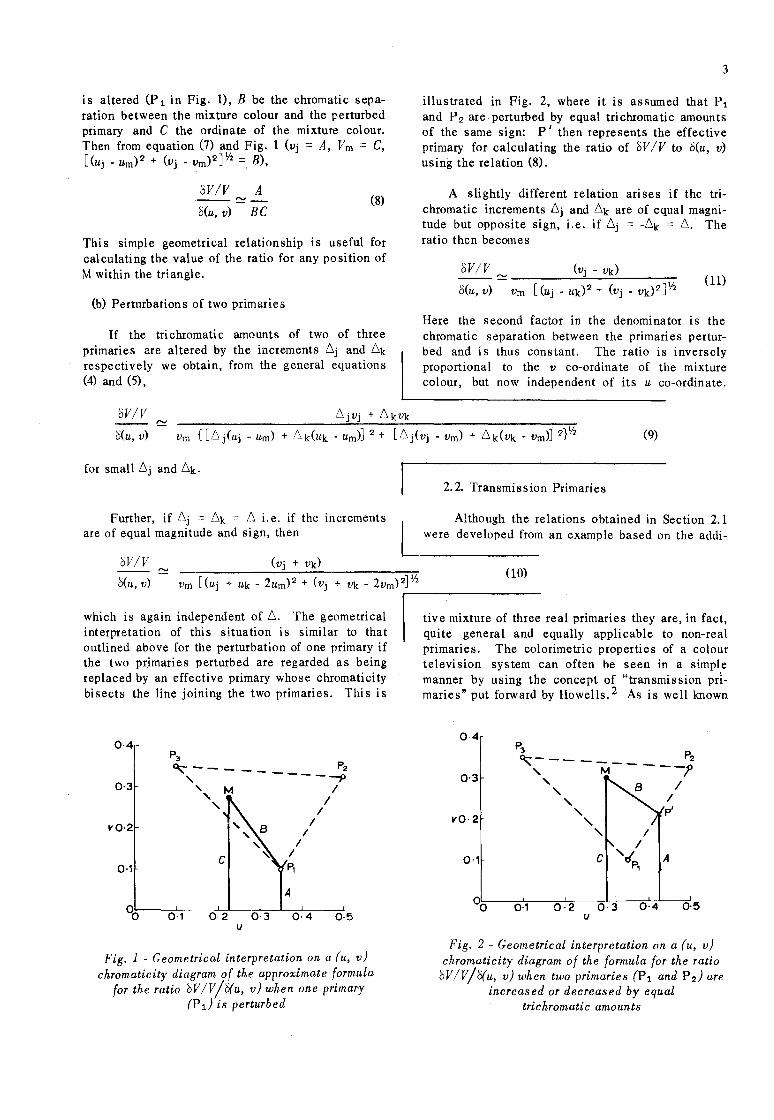
is altered (P 1 in Fig. 1), B be the chromatic sepa­ration between the mixture colour and the perturbed primary and C the ordinate of the mixture colour. Then from equation (7) and Fig. 1 (Vj :::: A, Vm :::: C, [(Uj - Urn) 2 + (Vj - Vm)2J Y2 :::: B),

OVIV A --~-o(U, v) BC

(8)

This simple geometrical relationship is useful for calculating the value of the ratio for any position of M within the triangle.

(b) Perturbations of two primaries

If the trichromatic amounts of two of three primaries are altered by the increments f':-.j and f':-.k respectively we obtain, from the general equations (4) and (5),

oVIV

o(u, v)

for small f':-.j and f':-.k.

Further, if f':-.j ::: f':-.k :::: f':-. i. e. if the increments are of equal magnitude and sign, then

~

3

illustrated in Fig. 2, where it is assumed that Pi and P 2 are perturbed by equal trichromatic amounts of the same sign: P I then represents the effective primary for calculating the ratio of OV IV to o(u, v) using the relation (8).

A slightly different relation arises if the tri­chromatic increments 6j and f':-.k are of equal magni­tude but opposite sign, i.e. if f':-.j == -f':-.k == f':-.. The ratio then becomes

_oV_I_V ~ (Vj - vk)

Vm [(Uj - Uk)2 + (Vj - Vk)2J Y2 (11)

o(U, v)

Here the second factor in the denominator is the chromatic separation between the primaries pertur­bed and is thus constant. The ratio is inversely proportional to the v co-ordinate of the mixture colour, but now independent of its U co-ordinate.

(9)

2.2. Transmission Primaries

Although the relations obtained in Section 2.1 were developed from an example based on the addi-

oVIV

o(u, v) Vm [(Uj + Uk - 2Um)2 + (Vj + Vk - 2Vm)2JV2 (10)

which is again independent of f':-.. The geometrical interpretation of this situation is similar to that outlined above for the perturbation of one primary if the two pr,imaries perturbed are regarded as being replaced by an effective primary whose chromaticity bisects the line joining the two primaries. This is

004

0·3

vO·2

0·1

P3 ~ -- _ _ _ P2 " -----p

, M / , / , /

/ I

I I c P,

A

u

Fig. 1 - Geometrical interpretation on a (u, v) chromaticity diagram of the approximate formula

for the ratio oV IV /O(u, v) when one primary (Pi) is perturbed

~----------------

tive mixture of three real primaries they are, in fact, quite general and equally applicable to non-real primaries. The colorimetric properties of a colour television system can often be seen in a simple manner by using the concept of "transmission pri­maries" put forward by Howells. 2 As is well known

0·4

0'3

vO·2

0·1

P3 ~-__ ____ _ P2

, M --?

0·1

, /

" / " , " , I

/ c 'r/..

P,

0·2 0·3 u

0·4

pi

A

(}5

Fig. 2 - Geometrical interpretation on a (u, v) chromaticity diagram of the formula for the ratio

oV IV /O(u, v) when two primaries (Pi and P 2 ) are increased or decreased by equal

trichromatic amounts

4

the R, G, and B decoded signal voltages applied to the display tube in a colour receiver control, res­pectively, the amounts of red, green and blue {phos­phor} primaries synthesizing the reproduced colour. At some earlier stage in the transmission process the three independent signals necessary to specify the reproduced colour may not control, respectively, the amounts of the reproducer primaries. Thus at this stage a perturbation of one of the signals may perturb the amounts of all three reproducer prima­ries. One can derive, however, an artificial set of primaries termed "transmis sion primaries" such that each one of the three signals at that stage in the transmission controls one and only one of the trans­mission primaries. The transmission primaries obey the same laws of colour mixture as do real primaries. The chromaticities of the transmission primaries, which may be unreal, can be derived from the three equations relating the amounts of the reproducer primaries to the signal voltages at the transmission stage under consideration. If these equations are linear then the chromaticities of the transmission primaries are independent of the repro­duced chroma tici ty. If the equations are non-linear then the chromaticities of the transmission primaries vary with the reproduced colour. To illustrate the above statements consider the transmission prima­ries of the NTSC colour television system for

(a) an ideal system (linear di splay tube) and

(b) the practical system (non-linear display tube)

/ ./

/ /

/

0'5

0·3

v

0·2 /'

/

/' 0,'

2.2.1. Linear System

In the NTSC sy stem the transmitted signals Ey, Er, and EQ are related to the signals applied to the di splay tube ER, Eo, and EB by the linear transformation (normalized so that if Ey = 1, Er = 0, EQ = 0 then ER = Eo = EB = 1).

r;:l 0 r: -::::: -:::::] r;~l (12)

l~~J l~ -1·106 1'703 l~Q In the ideal case, with a linear display tube

transfer characteristic, the signals ER, Eo, and EB will be related to the tristimulus values of the re­produced colour by the linear transformation

[~:] = k [:::: ::::: :::::11[::] (13)

Wm 0·145 0'827 0'62~J EB

where Urn, Vm, and Wm are the amounts of the C.I.E. - U.C.S.* reference stimuli, respectively, specifying the reproduced colour and k is a constant of proportionality.

* Uniform chromaticity scale.

~--------------------------------R~d

\

Blul2

\ \

\ // \

(I) / \(0) ~----~~~~~~----~~----~~ ______ -L ______ -L ______ -LI ______ ~I ______ ~~~ ______ ~

-0'5 -0-4 -0'3 -0·2 -0·' 0 0,' 0·2 0'3 0·4 u

Fig. 3 - Chromaticities of the NTSC transmission primaries and the reproducer primaties plotted on a (u, v) diagram

0·5

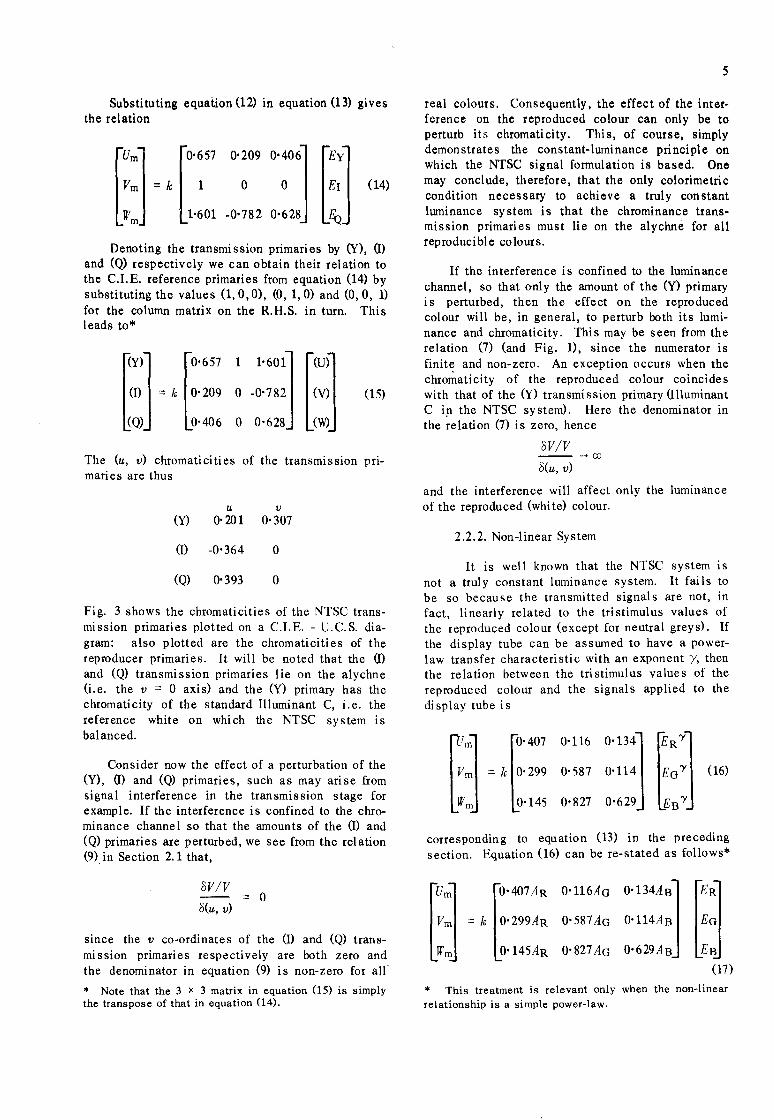
Substituting equation (12) in equation (13) gives the relation

[

urn] [0.657 Vm = k 1

W 1-601 m

0'209 0.406]

° ° -0'782 0'628

[j (14)

Denoting the transmission primaries by (Y), m and (Q) respectively we can obtain their relation to the C.I.E. reference primaries from equation (14) by substituting the values (1,0,0), (0, 1,0) and (0,0, 1) for the column matrix on the R.H.S. in turn. This leads to*

[

Y)] [0.657

(I) == k 0' 209

(Q) 0-406

: -:::::] [~)] ° 0-628 (W)

(15)

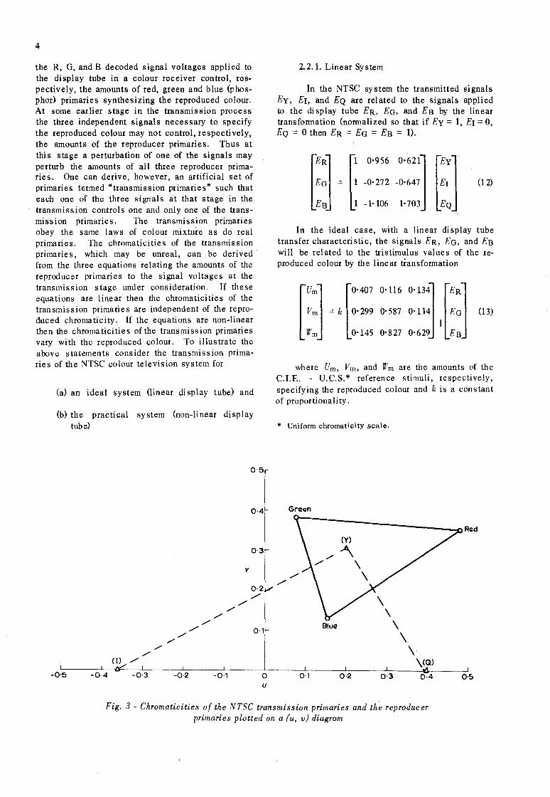
The (u, v) chromaticities of the transmission pri­maries are thus

u v (Y) 0-201 0'307

(I) -0-364 ° (Q) 0-393 o

Fig. 3 shows the chromaticities of the NTSC trans­mission primaries plotted on a C.I.E. - U.C.S. dia­gram: also plotted are the chromaticities of the reproducer primaries. It will be noted that the m and (Q) transmission primaries lie on the alychne (i.e. the v = 0 axis) and the (Y) primary has the chromaticity of the standard Illuminant C, i.e. the reference white on which the NTSC system is balanced.

Consider now the effect of a perturbation of the (Y), m and (Q) primaries, such as may arise from signal interference in the transmission stage for example. If the interference is confined to the chro­minance channel so that the amounts of the (I) and (Q) primaries are perturbed, we see from the relation (9) in Section 2.1 that,

bY/V

8(u, v} == ° since the v co-ordinates of the (I) and (Q) trans­mission primaries respectively are both zero and the denominator in equation (9) is non-zero for air

* Note that the 3 x 3 matrix in equation (15) is simply the transpose of that in equation (14).

5

real colours. Consequently, the effect of the inter­ference on the reproduced colour can only be to perturb its chromaticity. This, of course, simply demonstrates the constant-luminance principle on which the NTSC signal formulation is based. One may conclude, therefore, that the only colorimetric condition necessary to achieve a truly constant luminance system is that the chrominance trans­mission primaries must lie on the alychne for all reproducible colours.

If the interference is confined to the luminance channel, so that only the amount of the (y) primary is perturbed, then the effect on the reproduced colour will be, in general, to perturb both its lumi­nance and chromaticity. This may be seen from the relation (7) (and Fig. 1), since the numerator is finite and non-zero. An exception occurs when the chro~aticity of the reproduced colour coincides with that of the (y) transmission primary Ulluminant C ip the NTSC system). Here the denominator in the relation (7) is zero, hence

8V/V -- -+ (]J

8(u, v)

and the interference will affect only the luminance of the reproduced (white) colour.

2.2.2. Non-linear System

It is well known that the NTSC system is not a truly constant luminance system. It fails to be so because the transmitted signals are not, in fact, linearly related to the tristimulus values of the reproduced colour (except for neutral greys). If the display tube can be assumed to have a power­law transfer characteristic with an exponent 'I, then the relation between the tristimulus values of the reproduced colour and the signals applied to the display tube is

[

urn] [-407 Vm = k 0-299

Wm 0-145

0-134] tR

'Y] 0-114 Eo 'Y

0-629 EB 'Y

(16)

0-116

0-587

0'827

corresponding to equation (13) in the preceding section. Equation (16) can be re-stated as follows*

[j [~7AR 0'116Ao 0

0

134A B] ~:] Vm = k 0-299AR 0-587 Ao 0'114AB

Wm 0'145AR 0-827 Ao 0'629AB £B (17)

* This treatment is relevant only when the non-linear relationship is a simple power-law.

6

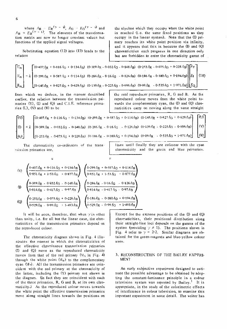
where AR == ER()' - 1>, AG == EG(Y - 1) and AB == EB(Y - i), The elements of the transforma­tion matrix are now no longer constant values but functions of the applied signal voltages.

Substituting equation (12) into (17) leads to the relation

the alychne which they occupy when the white point is reached (i.e. the same fixed positions as they occupy in the linear system). Note that the (I) pri­mary reaches its white point position via infinity, and it appears that this is because the (I) and <Q) chromaticities each progress in one direction only but are forbi dden to enter the chromati city gamut of

[

urn] [(0.407 A,R + 0-116AG + 0'134A8)

Vm == k (0-299AR + 0-587AG + 0-114AB)

Wm (0'145AR + 0-827AG + 0-629AB)

(0-389AR - o·o32AG - 0'148A8) (0-253AR - 0·075AG + 0'228AW]t']

(0'286AR - 0'16AG - 0'126AB) (0'186AR - 0'380AG + 0'194AB) El (8)

(0' 139AR - 0'225AG - 0'696AB) (0,09AR - 0·535AG + 1'071AB) E

from which we deduce, in the manner described earlier, the relation between the transmission pri­maries (Y), (I) and (Q) and c.l. E. reference prima­ries (U), (V) and (W) to be

the real reproducer primaries, R, G and B. As the reproduced colour moves from the white point to­wards the complementary cyan, the m and (Q) chro­maticities carry on moving along the same straight

,[:] = le

(V) [

0.407AR + 0'116AG + 0·134AB)

(0'389AR - 0'032AG - 0·148AB)

(0'253AR - 0'07504G + 0'228AB)

(0'299AR + 0'587AG + 0'11404B) (0'145AR + 0-827AG + 0.629A8)]

(0'28604R - 0-16AG - 0-126AB) (0'139AR - 0'225AG - 0·69604B)

(O'186AR - O'380AG + 0'19404B) (0,09AR - 0'535AG + 1'071AB)

The chromaticity co-ordinates of the trans- lines until finally they are colinear with the cyan mission primaries are, chromaticity and the green and blue primaries.

u v

(Y) (

0'407AR + 0'1l6AG + 0'134AB)

0'851AR + 1-53AG + 0'877AB (

0.299AR + 0'5R7AG + 0'114A8)

0'851AR + 1·53AG + 0·877AB

(

0.389AR - 0'Q32AG - 0'148AB)

0'814AR - 0-417AG - 0'97A8 (

0'286AR - 0'16AG - 0-126AB)

0'814AR - 0'417AG - 0'97AB

(Q) (

0'253AR - 0'075AG + 0'228AB)

0'529AR - 0'99AG + 1·493As (

0'186AR - 0-380AG + 0'194AB)

0-529AR - 0'99AG + 1-493A8

It will be seen, therefore, that when y is other than unity, i. e. for all but the line ar ca se, the chro­mati ci ti e s of the transmi s si on primari e s depend on the reproduced colour.

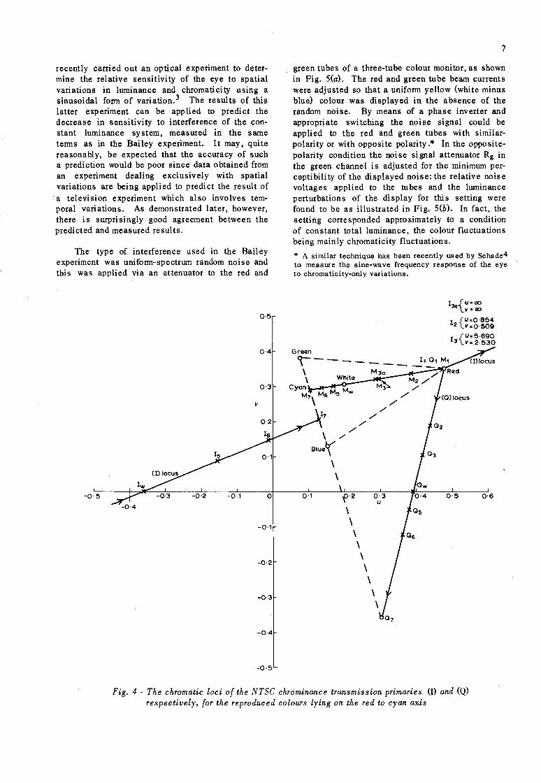
The chromaticity diagram shown in Fig. 4 illu­strates the manner in which the chromaticities of the effective chrominance transmission primaries (I) and (Q) move as the reproduced chromaticity moves from that of the red primary (M 1 in Fig. 4) through the white point (Mw) to the complementary cyan (M 7)' All the transmi ssion primari es are coin­cident with the red primary at the chromaticity of the latter, including the CY) primary not shown in the di agram. (In fact they are coincident wi th each of the three primaries, R, G and B, at its own chro­maticity.) As the reproduced colour moves towards the white point the effective transmission primaries move along straight lines towards the positions on

Except for the extreme positions of the m and (Q) chromaticities, their positionai distribution along their straight-line loci depends on the gamma of the system (providing y cj:. 1). The positions shown in Fig. 4 refer to y == 2· 2. Simi lar diagrams are ob­tained for the green-magenta and blue-yellow colour axes.

3. RECONSTRUCTION OF THE BAILEY EXPERI­MENT

An early subjective experiment designed to esti­mate the possible advantage to be obtained byadop­ting the constant-luminance principle in a colour televi sion sy stem was reported by Bai ley.1 It is appropriate, in the study of the colorimetric effects of interference in colour televi sion, to examine thi s important experiment in some detail. The writer has

recently carried out an optical experiment to deter­mine the relative sensitivity of the eye to spatial variations in luminance and chromaticity using a sinusoidal form of variation. 3 The results of this latter experiment can be applied to predict the decrease in sensitivity to interference of the con­stant luminance system, measured in the same terms as in the Bailey experiment. It may, quite reasonably, be expected that the accuracy of such a prediction would be poor since data obtained from an experiment dealing exclusively with spatial variations are being applied to predict the result of a television experiment which also involves tem­poral variations. As demonstrated later, however, there is surprisingly good agreement between the predicted and measured results.

The type of interference used in the Bailey experiment was uniform-spectrum random noise and this was applied via an attenuator to the red and

0-5

0-4

0-3

v

0-2

0-1

-0-5 -0'2 -0-1 o

-0-1

-0-2

-0-3

-0-4

-0,5

7

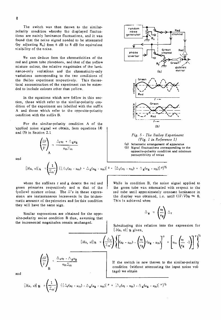
green tubes of a three-tube colour monitor, as shown in Fig. 5(a). The red and green tube beam currents were adjusted so that a uniform yellow (white minus blue) colour was displayed in the absence of the random noise. By means of a phase inverter and appropriate swi tching the noise signal could be applied to the red and green tubes with similar­polarity or with opposite polarity.* In the opposite­polarity condition the noise signal attenuator Rg in the green channel is adjusted for the minimum per­ceptibility of the displayed noise: the relative noise voltages applied to the tubes and the luminance perturbations of the di splay for thi s setting were found to be as illustrated in Fig. 5(b}. In fact, the setting corresponded approximately to a condition of constant total luminance, the colour fluctuations being mainly chromaticity fluctuation s.

... A similar technique has been recently used by Schade4 to measure the sine-wave frequency response of the eye to chromaticity-only variations.

Grlllln

<t-------_ \ _ M3a \ WhJtll~_~ • .,

Cyan M M M7\ Ms ~ w

17

0-1

\ \

f·2

\ \ \ \ \ \ \

0-3 U

\ \

13a{U.CC V" 00

I {UaO'8 54 2 v-O-SOg

I {Uc 5 .690 3 V=2-~30

0-5 0·6

Fig. 4 - The chromatic loci of the NTSC chrominance transmission primaries (I) and (Q) respectively, for the reproduced colours lying on the red to cyan ax.is

8

The switch was then thrown to the similar­polari ty condi tion whereby the di splayed fluctua­tions are mainly luminance fluctuations, and it was found that the noi se signal needed to be attenuated (by adjusting Rs) from 6 dB to 8 dB for equivalent visibility of the noise.

We can deduce from the chromaticities of the red and green tube phosphors, and that of the yellow mixture colour, the relative magnitudes of the lumi­nance-only variations and the chromaticity-only variations corresponding to the two conditions of the Bai ley experiment respectively. Thi s theore­tical reconstruction of the experiment can be exten­ded to include colours other than yellow.

In the equations which now follow in this sec­tion, those which refer to the similar-polarity con­dition of the experiment are labelled with the suffix A and those which refer to the opposite-polarity condition with the suffix B.

For the similar-polarity condition A of the 'appli ed noi se signal we obtain, from equation s (4) and (5) in Section 2.1

and

where the suffixes rand g denote the red and green primaries respectively and m that of the (yellow) mixture colour. The 6's in these expres­sions are instantaneous increments in the trichro­matic amounts of the primaries and for this condition they wi 11 have the same sign.

Similar expressions are obtained for the oppo­site-polarity noise condition B thus, assuming that the incremental magnitudes remain unchanged.

[o(u, v)] B

and

random nOise

genGlrotor

invczrtGlr

co u c o c "E "

Rczd channczi

(a) mirror

(b)

Fig. 5 - The Bailey Experiment (Fig. 1 in Reference 1)

Ca) Schematic arrangement of apparatus Cb) Signal fluctuations corresponding to the

opposite-polarity condition and minimum perceptibi lity of noise

While in condition B, the noise signal applied to the green tube was attenuated with respect to the red tube until approximately constant luminance in the di splay was obtained, i.e. until (bV /V)B ~ O. Thi s is achieved when

Substi tuting thi s rei ation into the expression for [o(u, v)] B gives,

If the switch is now thrown to the similar-polarity condition (without attenuating the input noise vol­tage) we obtain

and

26 rVr

2:mvm

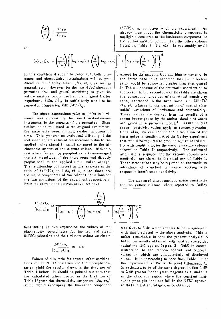
In this condition it should be noted that both lumi­nance and chromati city perturbations wi 11 be pro­duced in the di splay since [o(u~ v)] A is not, in general, zero. However, for the two NTSC phosphor primaries (red and green) combining to give the yellow mixture colour used in the original Bailey experiment [o(u, v)] A is sufficiently small to be ignored in compari son wi th (oV /V) A .

The above expressions refer to shifts in lumi­nance and chromaticity for small instantaneous increments in the amounts of the primaries. Since random noise was used in the original experiment, the increments were, in fact, random functions of time. This presents no analytical difficulty if the root mean square value of the increments due to the applied noise signal is small compared to the tri­chromatic amount of the mixture colour. With this restriction L. r can be regarded as a time-averaged (r.m. s.) magnitude of the increments and directly proportional to the applied r.m. s. noise voltage. The relationship of interest in this analysis is the ratio of (oV /V)A to [S(u, v)] B, since these are the major components of the colour fluctuations for the two conditions of the experiment respectively. From the expressions derived above, we have

(OV/V)A

[O(u, v)] B

Substituting in this expression the values of the chromaticity co-ordinates for the red and green (NTSC) primaries and their mixture colour we obtain

(OV/V)A

[o(u, V)]B 4-8

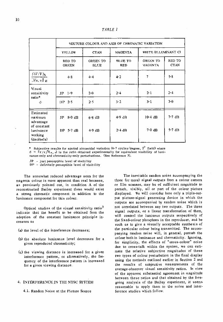
Values of this ratio for several other combina­tions of the NTSC primaries and their complemen­taries yield the results shown in the first row of Table 1 below. It should be pointed out here that the calculated ratios quoted in the first row of Table 1 ignore the chromaticity component [o(u~ v)AJ which would accompany the luminance component

9

(oV /V)A in condition A of the experiment. As already mentioned, the chromaticity component is negligible compared to the luminance component for the yellow mixture colour. For the other colours li sted in Table 1 [o(u, v),J is reasonably small

except for the magenta (red and blue primaries). In the latter case it is expected that the effective ratio would be somewhat greater than that quoted in Ta bl e 1 because of the chromati c contri bution to the noise. In the second row of this table are shown the corresponding values of the visual sensitivity ratio, expressed in the same terms i.e. (oV/V)! S(u, v), relating to the perception of spatial sinu-· soidal variations of luminance and chromaticity. These values are derived from the results of a recent investigation by the author, details of which are given in a previous report. 3 Assuming that these sensitivity ratios apply to random perturba­tions al so, we can deduce the attenuation of the input noise in condition A of the Bailey experiment that would be required to produce equivalent visibi­lity with condition B, for the various mixture colours (shown in Table 1) respectively. The estimated attenuations required, for the various colours res­pectively, are shown in the third row of Table 1. These attenuations may be regarded as the maximum advantage of constant luminance working with respect to interference sensi tivity.

The measured improvement in noise sensitivity for the yellow mixture colour reported by Bailey

was 6 dB to 8 dB which appears to be in agreement with that predicted by the above analysis. Thi s is rather remarkable in that the present analysi s is based on results obtained with spatial sinusoidal variations (6-7 cycles/degree, 2 0 field) in contra­di stinction to the random spatial and temporal variations which are characteristic of displayed noise. It is interesting to note from Table 1 that the improvement at the whi te point (Illuminant C) is estimated to be of the same degree, in fact 1 dB to 2 dB greater for the green-magenta axis, and this is the chromatic region where the constant lumi­nance principle does not fail in the NTSC system, so that the full advantage can be obtained.

10

TABLE 1

MIXTURE COLOUR AND AXIS OF CHROMATIC VARIATION

YELLOW CYAN MAGENTA WHITE (ILLUMINANT C)

RED TO GREEN TO BLUE TO GREEN TO RED TO

GREEN BLUE RED MAGENTA CYAN

(DV /V)A

[8(u, dB 4-8 4-4 4-2 7 5-8

Visual sensitivity JP 1-9 2-0 2-4 2-1 2-4 ratio*

cp DP 2-5 2-5 3-2 3-1 3-0

Estimated maximum JP 8-0 dB 6'8 dB 4-9 dB 10-4 dB 7-7 dB advantage of constant luminance DP 5-7 dB 4-9 dB 2-4 dB 7-0 dB 5-7 dB working (decibels)

'" Subjec~ive results for spatial sinusoidal variation (6·7 cycles/degree, 2° field) where <P ::: 0 V Iv lo( u, v) is the ratio obtained experimentally for equivalent visibility of lumi-nance-only and chromaticity-only perturbations. (See Reference 3).

JP - just percep~ible level of visibility DP - definitely perceptible level of visibility

The somewhat reduced advantage seen for the magenta colour is more apparent than real because, as previously pointed out, in condition A of the recon structed Bailey experiment there would exi st a strong chromatic component in addition to the luminance component for this colour.

Optical studies of the visual sensitivity rati03

indicate that the benefit to be obtained from the adoption of the constant luminance principle in­crease s as

(a) the level of the interference decreases;

(b) the absolute luminance level decreases for a given reproduced chromaticity;

(c) the viewing distance is increased for a given interferenc e pattern, or alternati vel y, the fre­quency of the interference pattern is increased for a given viewing distance.

4. INTERFERENCE IN THE NTSC SYSTEM

4.1. Random Noise at the Picture Source

The inevitable random noise accompanying the three (or more) signal outputs from a colour camera or film scanner, may be of sufficient magnitude to perturb, visibly, all or part of the colour picture displayed. We will consider here only a triple-out­put picture-signal generating device in which the outputs are accompanied by random noise which is not correlated between any two outputs. The three signal outputs, or a linear transformation of them, will control the luminous outputs respectively of the fixed-colour phosphors in the reproducer, and be such as to give a visually acceptable synthesi s of the particular colour being transmi tted. The accom­panying random noise will, in general, perturb the colour both in luminance and chromaticity. Ignoring, for simplicity, the effects of "cross-colour" noise due to cross-talk within the system, we can esti­mate the relative subjective magnitudes of these two types of colour perturbation in the final display using the methods outlined earlier in Section 2 and the results of subjective measurements of the average-observer visual sensitivity ratios. In view of the apparent substantial agreement in magnitude between these ratios and that obtained by the fore­going analysi s of the Bailey experiment, it seems reasonable to apply them to the noise and inter­ference studies which follow.

7

6

------------ ---"0

....

"0

"

'·0

Grczczn

............ ---

....

Blucz

.... " "

Rad

....

---- ---.-2 "3

--2 '3

............

2 "3

1 '3

---- -----o

_ saturation --

(a)

7

1 3 2 "0

'3 Mogcznto

-----

----

1 '3

-----------------o

_ saturation --

(b)

7

1 '3

2 '3 "0

YczllOW

---'--" ..... ~~~ ----------------

1 '3

o - saturation --

(C)

1 '3 eyan "0

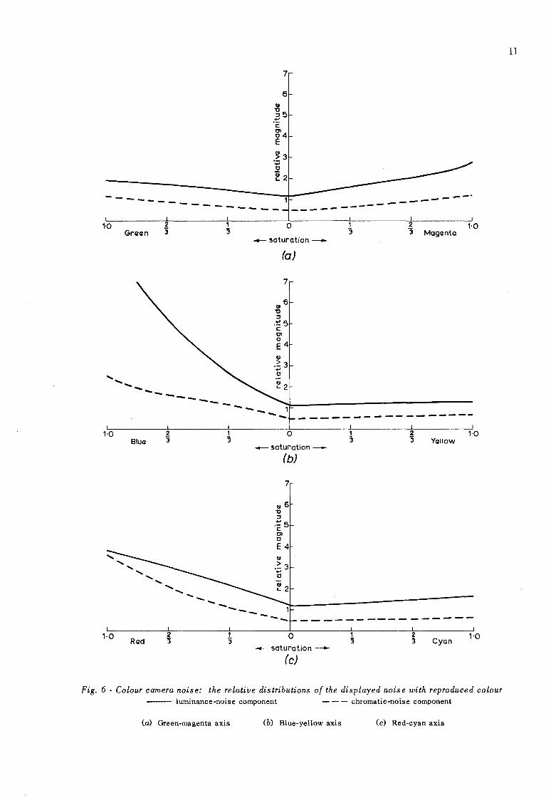
Fig. 6 - Colour camera noise: the relative distributions of the displayed noise with reproduced colour --- luminance-noise component - - - chromatic-noise component

(a) Green-magenta axis (b) Blue-yellow axis (c) Red-cyan axis

11

12

4.1.1. Colour Cameras

In the most usual situation the three signal outputs from the camera tubes are ER, Eo and EB, and are (approximately) directly proportional to the luminous outputs of the red, green and blue repro­ducer phosphors respectively. Hence, considered as effective transmission primaries, these signals will have chromaticities coincident with those of the (real) reproducer primaries for all reproducible colours. In a colour camera using image orthicon tubes or Plumbicon tubes, each signal will be accompanied by random noise, which may be con­sidered to be of constant power i.e. substantially independent of the signal level. By supposing that the signal-to-r.m.s. noise ratio is the same at each of the three camera outputs for the white-PQint (Illuminant C) (thi s is usually true for image ~rthi­cons, but not for Plumbicons), the relative distribu­tions of the resulting luminance-noi se and chroma­tic-noise with reproduced colour are shown in Fig. 6. In this figure the relative magnitude of each compo­nent is plotted against saturation* for the three

. primary colour-axes, green-magenta, red-cyan and blue-yellow respectively: the full lines refer to the luminance-noise component and the dashed lines to the chromatic-noi se component. In order to indi cate, approximately, the relative visual magnitudes of

'" Saturation is defined here as the ratio of the chromatic separation of the reproduced colour from Illuminant C to the maximum chromatic separation possible in the same direction, on the Uniform Chromaticity Scale. Thus all colours lying on the R, 0, 8 triangle have unit saturation.

040 Grczczn

035

030

v 0-25

0-20

0-15

Blucz

010 o 005 0-10 0-15 o 20 0-25

u

the components by the ratio of their ordinates in the figure it has been assumed (for simplicity) that the average-observer vi sual sensitivity ratio 8V Iv I 8(u, v) is 2' 5 : 1 for all chromatici ties. Thus equal ordinate values would imply equal visibilities of the two components, viewed separately. It should be pointed out that the vi sual sensitivity ratio does, in 'fact, increase with increasing magnitude of the perturbations. 3 Hence, referring to Fig. 6, toward the saturated blue and red colours, where the noise levels appear to increase markedly, too little weight has been given to the chromatic component in these regions by assuming a constant visual sensitivity ratio. Also, no account has been taken of variations of the ratio with luminance level. Hence the dia­grams shown indicate the relative visibilities of the two components for noise levels of such magnitude that, for a given reproduced colour, the chromatic­noise alone would be in the just perceptible class. It should be mentioned also that the analysis refers to the lower-frequency spectral components of the random noise, i.e. within the chrominance band­width .

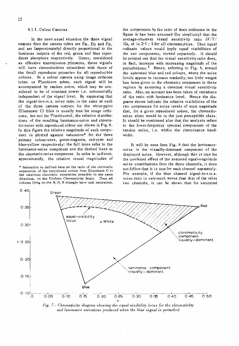
It will be seen from Fig. 6 that the luminance­noi se is the vi sually-dominant component of the displayed noise. However, although this is true for the combined effect of the assumed equal-magnitude noise contributions from the three channels, it does not follow that it is true for each channel separately. For example, if the blue channel signal-to-r.m. s. noise ratio is very much worse than that of the other two channels, it can be shown that for saturated

luminanccz componcznt visually- dominant

0-30 0-35 0040

chromaticity componcznt visually- dominant

0-45 050

Fig. 7 - Chromaticity diagram showing the equal-visibility locus for the chromaticity and luminance variations produced when the blue signal is perturbed

green, yellow, red and magenta colours the dominant component is likely to be' that of chromatic noi se. Fig. 7, for example, shows the chromatic region (hatched area) where perturbations of the blue sig­nal produce chromatic variations which are expected to be more visible than the luminance variations.

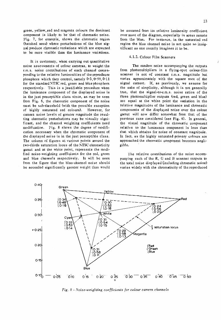
It is customary, when carrying out quantitative noise assessments of colour cameras, to weight the r.m. s. noi se contributions of each channel corres­ponding to the relative luminosities of the reproducer phosphors which they control, namely 0'3,0'59,0'11 for the standard NTSC red, green and blue phosphors respectively. This is a justifiable procedure when the luminance component of the displayed noise is in the just perceptible class since, as may be seen from Fig. 6, the chromatic component of the noi se must be sub-threshold (wi th the pos si ble exception of highly saturated red colours). However, for camera noise levels of greater magnitude the resul­ting chromatic perturbations may be visually signi­ficant, and the channel weighting coefficients need modification. Fig. 8 shows the degree of modifi­cation necessary when the chromatic component of the displayed noise is in the just perceptible class. The column of figures at various points around the two-thirds saturation locus of the NTSC chromatici ty gamut and at the white point, represents the modi­fied noi se-wei ghting coeffi ci ents for the red, green and blue channels re spectively. It wi 11 be seen from the figure that the blue-channel noise should be accorded significantly greater weight than would

0·4 Green

0·35

0'30

v 0-25

13

be assumed from its relative luminosity coefficient over most of the diagram, especially in areas remote from the blue, For instance, in the saturated red region the blue channel noise is not quite so insig­nificant as one usually imagines it to be.

4.1.2. Colour Film Scanners

The random noise accompanying the outputs from photomultipliers in a flying-spot colour-film scanner is not of constant r.m.s. magnitude but varies approximately with the square root of the si gnal current. If, as previously, we as sume for the sake of simplicity, although it is not generally true, that the signal-to-r.m.s. noise ratios of the three photomultiplier outputs (red, green and blue) are equal at the white point the variation in the relative magnitudes of the luminance and chromatic components of the displayed noise over the colour gamut will now differ somewhat from that of the previous case considered (see Fig. 6). In general, the vi sual magnitude of the chromatic component relative to the luminance component is less than that which obtains for noise of constant magnitude. In fact, as the highly saturated primary colours are approached the chromatic component becomes negli­gible.

The relative contributions of the noise accom­panying each of the R, G and B scanner outputs to the total noise displayed Gncluding chromatic noise) varies widely with the chromaticity of the reproduced

Red ----

/r ~ saturation locus

/' 0·58 /'~0'29 /' 0-13

/' /'

0·20 /' ,/ r~d GrlZlZn

BlulZ

0-15

BlulZ

0-100 0-05 0-10 0·15 0·20 0·25 0,30 0-35 0·40 0-45 0·50 u

F.ig. 8 - Noise-weighting coefficients for colour camera channels

14

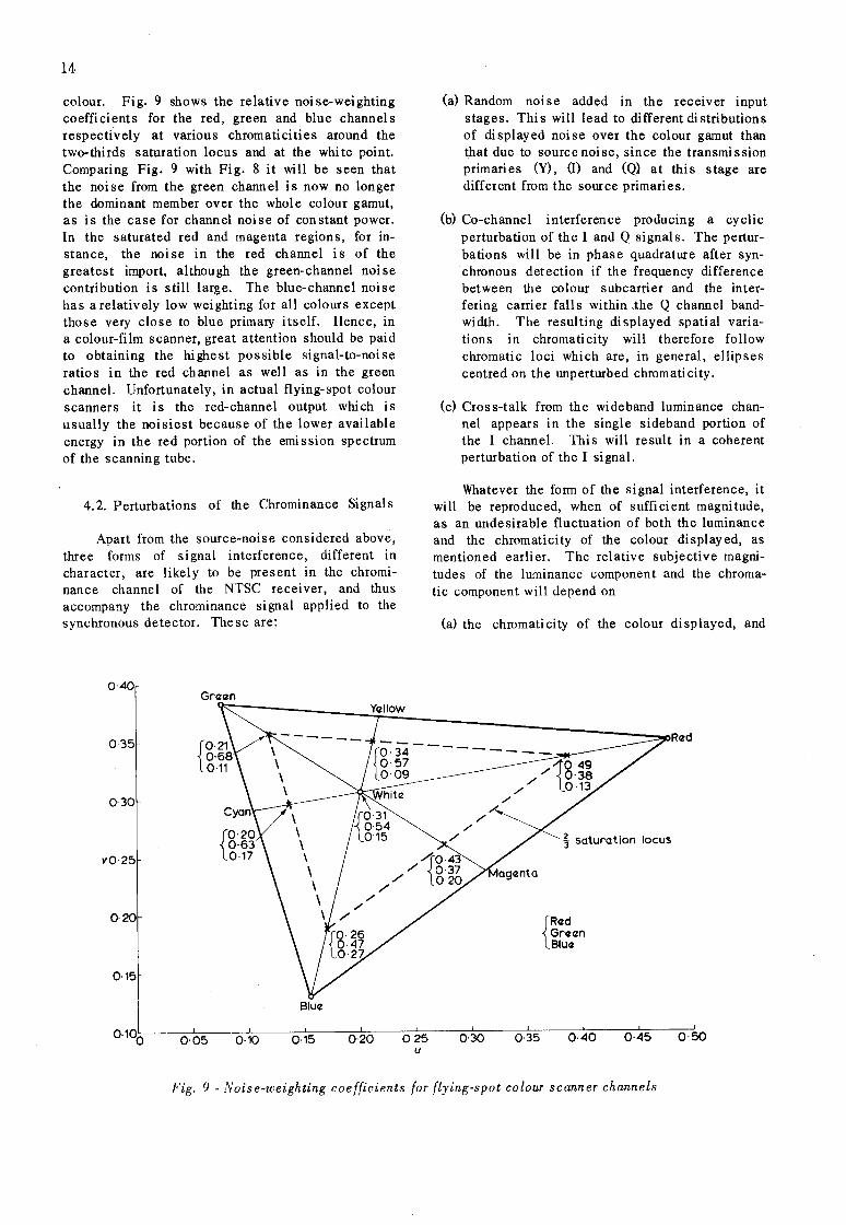
colour. Fig. 9 shows the relative noise-weighting coefficients for the red, green and blue channels respecti'vely at various chromaticities around the two-thirds saturation locus and at the whi te point. Comparing Fig. 9 with Fig. 8 it will be seen that the noise from the green channel is now no longer the dominant member over the whole colour gamut, as is the case for channel noise of constant power. In the saturated red and magenta regions, for in­stance, the noi se in the red channel is of the greates t import, although the green-channel noi se contribution is still large. The blue-channel noise has a relatively low weighting for all colours except those very close to blue primary itself. Hence, in a colour-film scanner, great attention should be paid to obtaining the highest possible signal-to-noise ratios in the red channel as well as in the green channel. Unfortunately, in actual flying-spot colour scanners it is the red-channel output which is usually the noisiest because of the lower available energy in the red portion of the emi ssion spectrum of the scanning tube.

4.2. Perturbations of the Chrominance Signal s

Apart from the source-noise considered above, three forms of signal interference, different in character, are likely to be present in the chromi­nance channel of the NTSC receiver, and thus accompany the chrominance signal applied to the synchronous detector. These are:

0,40 Graen

(a) Random noi se added in the receiver input stages. This will lead to different distributions of displayed noise over the colour gamut than that due to source noi se, since the transmi ssion primaries (Y), Q) and (Q) at this stage are different from the source primaries.

(b) Co-channel interference producing a cyclic perturbation of the I and Q signals. The pertur­bations will be in phase quadrature after syn­chronous detection if the frequency difference between the colour subcarrier and the inter­fering carrier falls within ,the Q channel band­width. The resulting di splayed spatial varia­tions in chromaticity will therefore follow chromatic loci which are, in general, ellipses centred on the unperturbed chromati city.

(c) Cros s-talk from the wideband luminance chan­nel appears in the single sideband portion of the I channel. This will result in a coherent perturbation of the I si gnal.

Whatever the form of the signal interference, it will be reproduced, when of sufficient magnitude, as an undesirable fluctuation of both the luminance and the chromaticity of the colour displayed, as mentioned earlier. The relative subjective magni­tudes of the luminance component and the chroma­tic component will depend on

(a) the chromaticity of the colour displayed, and

035 '\~~~~~~---Y~~----------------------------Rad

030

~ saturation locus

vO,25

0,20 rad Graan Blu(l

0,15

Blu(l

0,100

I I I I I I I I I

0,05 0,10 0,15 0·20 0·25 0·30 0·35 0·40 0·45 0·50 u

Fig. 9 - Noise-weighting coefficients for flying-spot colour scanner channels

(b) the visual sensitivity ratio (luminance/chro­maticity) appropriate to the particular form, angular size and level of the colourdisturbance produced.

Some indication was given in Section 3 of how the average-observer visual sensitivity ratio might be expected to vary with these latter factors. For instance, when the spatial disturbance is basically cyclic, say sinusoidal, the visual sensitivity ratio will increase with the angular size of the cycle or coarseness of the pattern.

It was deduced in Section 3 that the visual sen­sitivi ty ratio {defined as the ratio of (oV /V)r.m.s. to o(u, v)r.m.s. for equal visibility of each compo­nent) for coloured random noi se, probably lies in the range 2 : 1 to 3 : 1, the actual value wi thin the range depending to some extent on the level of the noi se above threshold and the mean chromaticity of the colour. However, for brevity in the analysis which follows, it is assumed that the visual sen­si tivi ty ratio has a constant val ut! of 2' 5 : 1 for all forms of interference.

(Crl+CI2)t

'" '0

e

~ 7 ';: '" " E

5

x, \. __ -

1 ..... ----- 4

,-./ Ca

1_-,,--- - - ----.

__ """""--3 ---2

15

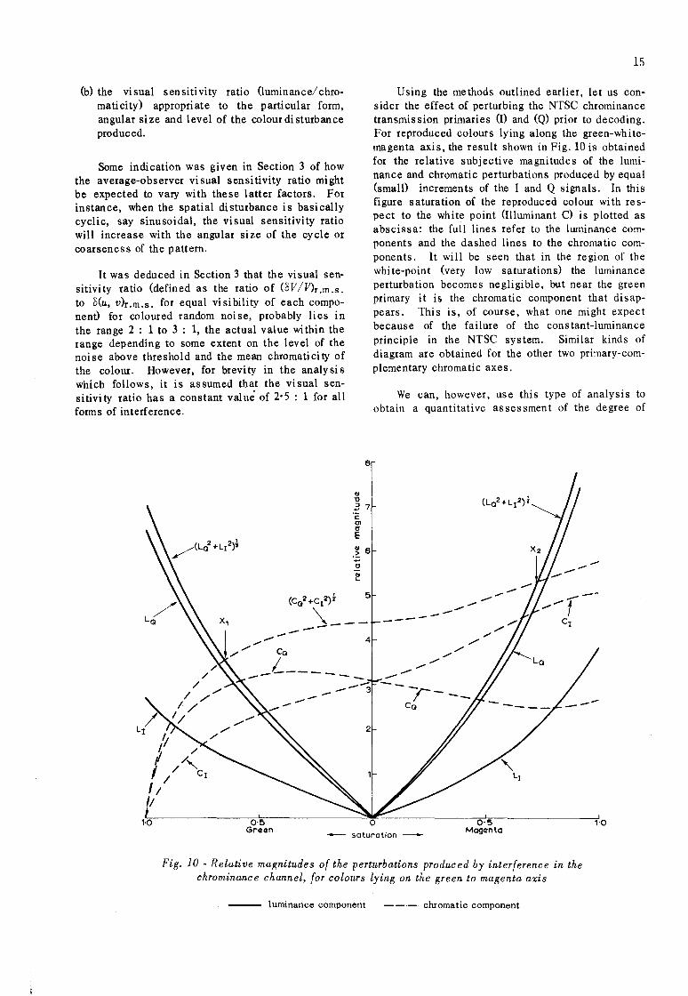
Using the methods outlined earlier, let us con­sider the effect of perturbing the NTSC chrominance transmis sion primaries (I) and (Q) prior to decoding. For reproduced colours lying along the green-white­magenta axis, the result shown in Fig. 10 is obtained for the relative subjective magnitudes of the lumi­nance and chromatic perturbations produced by equal (small) increments of the I and Q signals. In this figure saturation of the reproduced colour with res­pect to the white point (Illuminant C) is plotted as abscissa: the full lines refer to the luminance com­ponents and the dashed lines to the chromatic com­ponents. It will be seen that in the region of the white-point (very low saturations) the luminance perturbation becomes negligible, but near the green primary it is the chromatic component that disap­pears. This is, of course, what one might expect because of the failure of the cons tant-Iuminance principle in the NTSC system. Similar kinds of diagram are obtained for the other two primary-com­plementary chromatic axes.

We can, however, use this type of analysis to obtain a quantitative assessment of the degree of

---

--------

./ ,./

",­",-

--1-- ---­Ca

---, --Cl

',0 o 0·5 Grczczn

- saturation

0'5 Magcznta

Fig. 10 - Rel~tive magnitudes of the perturbations produced by interference in the chrommanc e channel, for colours lying on the green to magenta axis

--- luminance component -- - chromatic component

16

failure of the constant-luminance principle and so provide, perhaps, a more realistic meaning to the more commonly used measure - the constant lumi­nance index. Suppose, for instance, that we con­sider the constant-luminance principle to have "failed" when a given amount of interference in the chrominance channel produce s chromatic and lumi­nance perturbations that (could they be viewed separately) would be of equal subjective magni tude. Referring to Fig. 10 this would occur at the chroma­ticities corresponding to the cross-over points marked X 1 on the green side, and X:2 on the magenta side. *

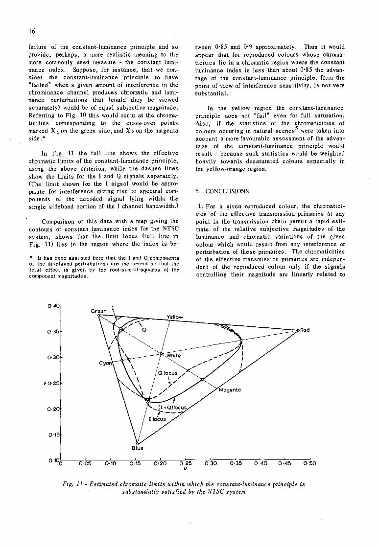
In Fig. 11 the full line shows the effective chromatic limi ts of the cons tant-luminance principle, using the above criterion, while the dashed lines show the limits for the I and Q signals separately. (The limit shown for the I signal would be appro­priate for interference giving rise to sp'ectral com­ponents of the decoded signal lying within the single sideband portion of the I channel bandwidth,)

Comparison of this data with a map giving the contours of constant luminance index for the NTSC system, .shows that the limit locus (full line in Fig. 11) lies in the region where the index is be-

* It has been assumed here that the I and Q components of the displayed perturbations are incoherent so that the total effect is given by the root-sum-of-squares of the component magnitudes.

0·40

0·35

0·30

vO'25

0·20

0·15

BlutZ

tween 0'85 and 0'9 approximately. Thus it would appear that for reproduced colours whose chroma­ticities lie in a chromatic region where the constant luminance index is less than about 0'85 the advan­tage of the constant-luminance principle, from the point of view of interference sensitivity, is not very substantial.

In the yellow region the constant-luminance principle does not "fail" even for full saturation. Also, if the statistics of the chromaticities of colours occuring in natural scenes 5 were taken into account a more favourable assessment of the advan­tage of the constant-luminance principle would result - because such statistics would be weighted heavily towards desaturated colours especially in the yellow-orange region.

5. CONCLUSIONS

1. For a given reproduced colour, the chromatic i­ties of the effective transmission primaries at any point in the transmission chain permit a rapid esti­mate of the relative subjective magnitudes of the luminance and chromatic variations of the given colour which would result from any interference or perturbation of these primaries. The chromaticities of the effective transmission primaries are indepen­dent of the reproduced colour only if the signals controlling their magnitude are linearly related to

0·~0~---0~·~0~5--~0~·~10~--0~·~15~--70~·2~0~~0~·~25~--70~·3~0--~0~.3~5~~0~·~4~0---0~·4~5--~0~·50 u

Fig. 11 - Estimated chromatic limits within which the constant-luminance principle is substantially satisfied by the NTSC system

l

the tristimulus values of the colour. If not so re­lated, their chromatic positions vary with the re pro-

,duced colour. Further, if the relation is a power law of exponent y(:;t!: 1), then for any straight-line locus of reproduced chromaticities there is a corres­ponding straight-Line locus for each of the trans­mission primaries and the direction of these loci is independent of the value of y.

2. Theoretical re-examination of the early Bailey experiment reveals that the vi sua I sensitivity ratio [( OV /V)/ o(u, v)] for coloured random noise is in the range 2 : 1 to 2·5 : 1, for the yellow mixture colour used in the original experiment. This result appears to be in remarkable agreement wi th recent subjective measurements of the visual sensitivity ratio for this colour using spatial, sinusoidal variations (6·7 cycles/degree) in an optical experiment. 3

3. The displayed noise in a colour receiver, due to noise which originates at the picture source can have a substantial chromatic component in some regions of colour, although the luminance component will usually be the larger. In assessing the relative contributions to the total noise from the signal-to­noise ratios of the three outputs from a conventional camera or film-scanner, the usual noise-weighting coefficients, based on the relative luminosities of the reproducer primaries, need some modification if the chromatic component is above the threshold of visibility. In a camera, for instance, the noise in the blue channel should be accorded more weight than the relative luminosity coefficient of the blue primary would indicate. In a flying-spot scanner the noise from the red channel is perhaps of greater import than the relative luminosity of the red pri­mary would indicate.

CHD

17

4. It is estimated that the cons tant-Iuminance prin­ciple "fails" for those colours lying in the border region of the total chromaticity gamut where the constant luminance index is less than about 0·85. This estimate is based on the criterion that the principle "fai Is" when interference in the chromi­nance channel produces luminance and chromatic fluctuations of equal subjective magnitude, and on the assumption that the visual sensitivity ratio is 2·5 : 1.

6. REFERENCES

1. BAILEY, W.F.: "The Constant Luminance Prin­ciple in NTSC Colour Television", Proc. lnst. Radio Engrs., 1954, 42, 1, pp. 60 - 66.

2. HOWELLS, P. W.: "The Concept of Transmission Primaries in Colour Television", Proc. lnst. Radio Engrs., 1954, 42, 1, pp. 134 - 138.

3. "The Relative Visibilities of Spatial Variations in Luminance and Chromaticity", Research Department Report No. T-146, Serial No. 1965/24.

4. SCHADE, O.H.: "On the Quality of Colour Tele­vision Images and Perception of Colour Detail", J. Soc. \1otion Pict. Telev. Engrs., 67, 12, 1958, pp. 801 - 819.

5. MacADA\1, D.L.: "Reproduction of Colour in Outdoor Scenes", Proc. lnst. Radio Engrs., 1954, 42, 1, pp. 166 - 174.

Printed by BBC Research Department, Kingswood Warren, Tadworth, Surrey