1

Color Demosaicing Using Variance of Color Differences

King-Hong Chung and Yuk-Hee Chan1

Centre for Multimedia Signal Processing Department of Electronic and Information Engineering The Hong Kong Polytechnic University, Hong Kong

ABSTRACT This paper presents an adaptive demosaicing algorithm. Missing green samples are first

estimated based on the variances of the color differences along different edge directions. The missing red and blue components are then estimated based on the interpolated green plane. This algorithm can effectively preserve the details in texture regions and, at the same time, it can significantly reduce the color artifacts. As compared with the latest demosaicing algorithms, the proposed algorithm produces the best average demosaicing performance both objectively and subjectively.

EDICS: ISR-INTR Interpolation; RST-OTHR Other

1 Corresponding author (Email: enyhchan@polyu.edu.hk)

2

I. INTRODUCTION

A full-color image is usually composed of three color planes and, accordingly, three separate sensors are required for a camera to measure an image. To reduce the cost, many cameras use a single sensor covered with a color filter array (CFA). The most common CFA used nowadays is the Bayer CFA shown in Fig. 1 [1]. In the CFA-based sensor configuration, only one color is measured at each pixel and the missing two color values are estimated. The estimation process is known as color demosaicing [2].

In general, a demosaicing algorithm can be either heuristic or non-heuristic. A heuristic approach does not try to solve a mathematically defined optimization problem while a non-heuristic approach does. Examples of non-heuristic approaches include [3-6]. In particular, Gunturk’s algorithm (AP) [3] tries to maintain the output image within the “observation” and “detail” constraint sets with the Projection-Onto-Convex-Sets (POCS) technique while Muresan’s algorithm (DUOR) [4] is an optimal-recovery-based nonlinear interpolation scheme. As for the one in [5] (DSA), it successfully approximates the demosaicing result in color difference domain with a spatially adaptive stopping criterion. Alleyson’s algorithm [6] proposed a low-pass and a corresponding high-pass filter for recovering the luminance and chrominance terms via analyzing the characteristics of a CFA image in frequency domain.

Most existing demosaicing algorithms are heuristic algorithms. Bilinear interpolation (BI) [7] is the simplest heuristic method, in which the missing samples are interpolated on each color plane independently and high frequency information cannot be preserved well in the output image. With the use of inter-channel correlation, algorithms proposed in [8-11] attempt to maintain edge detail or limit hue transitions to provide better demosaicing performance. In [12], an effective color interpolation method (ECI) is proposed to get a full color image by interpolating the color differences between green and red/blue plane. The algorithms proposed in [13-22] are some of the latest methods. Among them, Wu’s algorithm [13] is a primary-consistent soft-decision (PCSD) algorithm which eliminates color artifacts by ensuring the same interpolation direction for each color component of a pixel while Hirakawa’s algorithm (AHDDA) [15] uses local homogeneity as an indicator to pick the direction for interpolation. In [16-18,20-22], a color-ratio model or a color-difference model cooperating with an edge-sensing mechanism is used to drive the interpolation process along the edges while, in [19], an adaptive demosaicing scheme using bilateral filtering technique is proposed.

To a certain extent, it can be found that a number of heuristic algorithms were developed based on the framework of the adaptive color plane interpolation algorithm (ACPI) proposed in [10]. For examples, algorithms in [13] and [15] exploit the same interpolators used in ACPI to generate the green plane. The improved demosaicing performance of these advanced heuristic algorithms is generally achieved by that they can interpolate the missing samples along a correct direction. In this paper, based on the framework of ACPI, a new heuristic demosaicing algorithm is proposed. This algorithm uses the variance of pixel color differences to determine the interpolation direction for interpolating the missing green samples. Simulation results show that the proposed algorithm is superior to the latest demosaicing algorithms in terms of both subjective and objective criteria. In particular, it can outstandingly preserve the texture

3

details in an image. The paper is organized as follows. In Section II, we revisit the ACPI algorithm [10]. An analysis is

made and our motivation to develop the proposed algorithm is presented. Section III presents the details of our demosaicing algorithm and Section IV presents some simulation results for comparison study. Finally, a conclusion is given in Section V.

II. OBSERVATIONS ON THE ADAPTIVE INTERPOLATION ALGORITHM

In ACPI [10], the green plane is handled first and the other color planes are handled based on the estimation result of the green plane. When the green plane is processed, for each missing green component in the CFA, the algorithm performs a gradient test and then carries out an interpolation along the direction of a smaller gradient to determine the missing green component. A pixel without green component in the Bayer CFA may have a neighborhood as shown in either Fig. 1a or Fig. 1b. Without losing the generality, here we consider the former case only. In this case, the horizontal gradient jiH ,Δ and the vertical gradient jiV ,Δ at position (i,j) are estimated first to determine the interpolation direction

as follows.

2,2,,1,1,, 2 +−+− −−+−=Δ jijijijijiji RRRGGH (1)

jijijijijiji RRRGGV ,2,2,,1,1, 2 +−+− −−+−=Δ (2)

where Rm,n and Gm,n denote the known red and green CFA components at position (m,n). Based on the values of jiH ,Δ and jiV ,Δ , the missing green component gi,j in Fig. 1a is interpolated as follows.

jijijijijijiji

ji VHRRRGG

g ,,2,2,,1,1,

, if4

)2(2

)(Δ<Δ

−−+

+= +−+− (3)

jijijijijijiji

ji VHRRRGG

g ,,,2,2,,1,1

, if4

)2(2

)(Δ>Δ

−−+

+= +−+− (4)

8)4(

4)( 2,2,,2,2,1,1,,1,1

,+−+−+−+− −−−−

++++

= jijijijijijijijijiji

RRRRRGGGGg

if jiji VH ,, Δ=Δ (5) In fact, it was shown in [15] that eqns. (3) and (4) were the approximated optimal CFA interpolators in horizontal and vertical directions and eqn. (5) was good enough for interpolating diagonal image features.

Since the red and the blue color planes are determined based on the estimation result of the green plane and the missing green components are in turns determined by the result of the gradient test, the demosaicing result highly relies on the success of the gradient test. A study was performed here to evaluate how significant the gradient test is to the performance of the algorithm.

In a simulation of our study, twenty-four 24-bit (of bit ratio R:G:B=8:8:8) digital color images of size 512×768 pixels each as shown in Fig. 2 were sampled according to Bayer CFA to form a set of testing images. These images are part of the Kodak color image database and include various scenes. The

4

testing images were reconstructed with ACPI [10] and the ideal ACPI. The ideal ACPI is basically ACPI except that, in determining a missing green component, it computes all gi,j estimates with eqns.(3)-(5) and picks the one closest to the real value of the missing component without performing any gradient test. Note that in this simulation all original images are known and hence the real value of a missing green component of the testing images can be used to implement the ideal ACPI. In practice, the original images are not known and hence the performance of the ideal ACPI is practically unachievable. The ideal ACPI is only used as a reference in our study.

We measured the peak signal-to-noise ratios (PSNRs) of the interpolated green planes of both ACPI [10] and the ideal APCI with respect to the original green plane. We found that the average PSNR achieved by the ideal ACPI was 43.83dB while that achieved by ACPI was only 38.18dB. This implies that there is a great room for improving the performance of ACPI. Based on this simulation result, we have two observations. First, the interpolators used in [10] can be very effective if there is an ‘effective’ gradient test to provide some reliable guidance for the interpolation. Second, the current gradient test used in [10] is not good enough.

After having the ‘ideal’ green plane with the ideal ACPI, we proceeded to interpolate the red and the blue planes with it to produce a full color image with the same procedures as originally proposed in ACPI. The quality of the output was measured in terms of color-peak signal-to-noise ratio (CPSNR) which is defined in eqn.(24). As expected, it achieves extremely high score and, subjectively, it is hard to distinguish the recovered image from the original full color image. Table 1 shows the performance of various algorithms for comparison. As shown in Table 1, the ideal ACPI provides a very outstanding performance as compared with any other evaluated demosaicing algorithms. This shows that the approach used in [10] to derive the other color planes with a ‘good’ green plane is actually very effective. As a good green plane relies on a good gradient test, the key of success is again the effectiveness of the gradient test or, to be more precise, the test for determining the interpolation direction. This finding motivates the need to find an effective and efficient gradient test to improve the performance of ACPI.

When we probed into the gradient test used in [10], we found that the test encountered problems when dealing with pixels in texture regions. Fig. 3 shows an example where the test does not work properly. A 5×5 block located in a texture region is extracted for inspection as shown in Fig. 3a. Fig. 3b and Fig. 3c show, respectively, the pixel values of the vertical and the horizontal lines across the block center. Suppose the black dots in the plots are the CFA samples while the others are the samples needed to be estimated. Consider that we are going to estimate the green component of the block center. As the black dash lines in vertical direction are flatter than that in horizontal direction, the test provides a misleading result. The algorithm interpolates vertically to determine the missing green component although it should interpolate horizontally. That is the reason why details cannot be preserved in a texture region with ACPI.

In summary, the ACPI algorithm can perform outstandingly if all the missing green samples are interpolated in appropriate directions. Thus, the determination of the interpolation direction for the missing green samples, in turn, becomes the ghost of the demosaicing method.

5

III. PROPOSED ALGORITHM

Based on the observations presented in Section II, the proposed algorithm put its focus on how to effectively determine the interpolation direction for estimating a missing green component in edge regions and texture regions. In particular, variance of color differences is used in the proposed algorithm as a supplementary criterion to determine the interpolation direction for the green components.

For the sake of reference, hereafter, a pixel at location (i,j) in the CFA is represented by either (Ri,j, gi,j, bi,j), (ri,j, Gi,j, bi,j) or (ri,j, gi,j, Bi,j), where Ri,j, Gi,j and Bi,j denote the known red, green and blue components and ri,j, gi,j and bi,j denote the unknown components in the CFA. The estimates of ri,j, gi,j and

bi,j are denoted as jiR ,ˆ , jiG ,

ˆ and jiB ,ˆ . To get jiR ,

ˆ , jiG ,ˆ and jiB ,

ˆ , preliminary estimates of ri,j, gi,j and

bi,j may be required in the proposed demosaicing algorithm. These intermediate estimates are denoted as

jir ,ˆ , jig ,ˆ and jib ,ˆ .

A. Interpolating Missing Green Components

In the proposed algorithm, the missing green components are first interpolated in a raster scan manner. As far as a missing green component in the Bayer CFA is concerned, its neighborhood must be in a form as shown in either Fig. 1a or Fig. 1b. Without losing the generality, let us consider the case shown in Fig. 1a only. For the other case, the same treatment used in this case can be done to estimate the missing green component by exchanging the roles of the red components and the blue components.

In Fig. 1a, the center pixel pi,j is represented by (Ri,j, gi,j, bi,j), where gi,j is the missing green component needed to be estimated. The proposed algorithm computes the two following parameters instead of jiH ,Δ and jiV ,Δ as in ACPI algorithm.

∑ ∑∑

∑ ∑∑

±= ±=+++

±=+++

±= ±=+++

±=+++

⎥⎥⎦

⎤

⎢⎢⎣

⎡−+−+

⎥⎥⎦

⎤

⎢⎢⎣

⎡−+−=

1 1,,

2,0,,

2 1,,

2,0,,

n mjminjmi

mjminjmi

n mjminjmi

mjminjmi

H

GBRG

GGRRL

(6)

∑ ∑∑

∑ ∑∑

±= ±=+++

±=+++

±= ±=+++

±=+++

⎥⎥⎦

⎤

⎢⎢⎣

⎡−+−+

⎥⎥⎦

⎤

⎢⎢⎣

⎡−+−=

1 1,,

2,0,,

2 1,,

2,0,,

m nnjinjmi

nnjinjmi

m nnjinjmi

nnjinjmi

V

GBRG

GGRRL

(7)

These two parameters are used to estimate whether there is sharp horizontal or vertical gradient

change in the 5×5 testing window (with pi,j as the window center). A large value implies that there exists a sharp gradient change along a particular direction. The ratio of the two parameters is then computed to determine the dominant edge direction.

6

),max( V

H

H

V

LL

LLe = (8)

A block is defined to be a sharp edge block if e>T, where T is a predefined threshold value to be

discussed in more details in Section IV. If a block is a sharp edge block, the missing green component of the block center is interpolated as follows.

Vjijijijijiji LL

RRRGGg <

−−+

+= +−+− H2,2,,1,1,

, if4

)2(2

)( (9)

Vjijijijiji

ji LLRRRGG

g >−−

++

= +−+− H,2,2,,1,1, if

4)2(

2)(

(10)

The block classifier based on eqns. (6-8) and threshold T is used to detect sharp edge blocks and

determine the corresponding edge direction for interpolation. In eqns. (6) and (7), both inter-band and

intra-band color information is used to evaluate parameters VL and HL . The first summation terms of eqns. (6) and (7) contribute the intra-band information, which involves the difference between a pixel and its second next pixel. Obviously, the resolution that it supports cannot detect a sharp line of width 1 pixel. The supplementary intra-band color information contributed in the second summation terms of eqns. (6) and (7) is used to improve the resolution of the edge detector.

A block which is not classified to be an edge block is considered to be in a flat region or a pattern region. It was found that, in a local region of a natural image, the color differences of pixels are more or less the same [23]. Accordingly, the variance of color differences can be used as supplementary information to determine the interpolation direction for the green components.

In the proposed algorithm, we extend the 5×5 block of interest into a 9×9 block by including more neighbors as shown in Fig. 4 and evaluate the color differences of the pixels along the axis within the 9×9

window. Let 2, jiHσ and 2

, jiV σ be, respectively, the variances of the color differences of the pixels along

the horizontal axis and the vertical axis of the 9×9 block. In particular, they are defined as

22

91

91 ∑ ∑

Ψ∈ Ψ∈++ ⎟

⎟⎠

⎞⎜⎜⎝

⎛−=

n kkjinjijiH dd ,,,σ (11)

and 2

291

91 ∑ ∑

Ψ∈ Ψ∈++ ⎟

⎟⎠

⎞⎜⎜⎝

⎛−=

n kjkijnijiV dd ,,,σ (12)

where dp,q is the color difference of pixel (p,q) and },,,,{ 43210 ±±±±=Ψ is a set of indexes which helps

to identify a pixel in the 9×9 support region. The values of di,j+n and di+n,j for Ψ∈n should be

pre-computed and they are determined sequentially as follows.

7

⎩⎨⎧

=−−−=−=

++

+++ 420 if

42 if,,ˆ,ˆ

,,

,,, ngR

nGRdnjinji

njinjinji (13)

⎩⎨⎧

=−−−=−=

++

+++ 420 if

42 if,,ˆ,ˆ

,,

,,, ngR

nGRdjnijni

jnijnijni (14)

3,1for 2/)( 1,1,, ±±=+= ++−++ nddd njinjinji (15)

and 3,1for 2/)( ,1,1, ±±=+= ++−++ nddd jnijnijni (16)

Here, bilinear interpolation is used with the concern about the realization complexity to estimate njid +,

and jnid ,+ for 31 ±±= , n . In fact, there was no obvious improvement in the simulation results when

other interpolation schemes such as cubic interpolation were used. To provide some more information about eqns.(13) and (14), we note that the missing green

components are estimated in a raster scan fashion and hence the final estimates of the green components in position },|),(),,{(, 42 −−=++=Ω njninjiji are already computed. As for the missing green components of the pixels in position },,|),(),,{( 420=++ njninji , their preliminary estimates njig +,ˆ and jnig ,ˆ + have to be evaluated. Specifically, njig +,ˆ is determined with eqn.(3) while jnig ,ˆ + is determined with eqn.(4) unconditionally. Note the di,j involved in eqn.(11) uses the jig ,ˆ determined with eqn.(3) while the di,j involved in eqn.(12) uses the jig ,ˆ determined with eqn.(4).

The variance of the color differences of the diagonal pixels in the 9×9 window, say 2, jiBσ , are

determined by

⎟⎟

⎠

⎞

⎜⎜

⎝

⎛⎟⎟⎠

⎞⎜⎜⎝

⎛−+⎟⎟

⎠

⎞⎜⎜⎝

⎛−= ∑ ∑∑ ∑

Ψ∈ Ψ∈++

Ψ∈ Ψ∈++

2

,,

2

,,2, 9

191

91

91

21

n kkjinji

n kjkijnijiB ddddσ (17)

The same set of eqns.(13)-(16) are used to get the color difference dp,q required in the evaluation of 2, jiBσ .

However, the preliminary estimates njig +,ˆ and jnig ,ˆ + involved in these equations are determined with

eqn. (5) instead of eqns. (3) and (4). Finally, the interpolation direction for estimating the missing green component at pi,j=(Ri,j, gi,j, bi,j)

can be determined based on 2, jiHσ , 2

, jiV σ and 2, jiBσ . It is the direction providing the minimum

variance of color difference. The missing green gi,j can then be estimated with either formulation (3), (4) or (5) without concerning jiH ,Δ and jiV ,Δ as follows.

8

⎪⎪⎩

⎪⎪⎨

⎧

=

=

=

=

) min(if (5) ofresult evaluation nalunconditio

) min(if (4) ofresult evaluation nalunconditio

) min(if (3) ofresult evaluation nalunconditioˆ

2222

2222

2222

,

i,jBi,jVi,jHi,jB

i,jBi,jVi,jHi,jV

i,jBi,jVi,jHi,jH

ji

σ,σ,σσ

σ,σ,σσ

σ,σ,σσ

G (18)

Once the missing green component is interpolated, the same process is performed for estimating the next missing green component in a raster scan manner. For estimating the missing green component in the case shown in Fig. 1b, one can replace the red samples by the corresponding blue samples and follow the procedures above to determine its interpolation direction and its interpolated value.

The complexity of the realization of eqn. (18) and its preparation work (eqns. (11)-(17)) is large. When e>T, a sharp edge block is clearly identified. In that case, using eqns. (9) and (10) to interpolate missing components can save a lot of effort and, at the same time, provide a good demosacing result. B. Interpolating Missing Red and Blue Components at Green CFA sampling positions

After interpolating all missing green components of the image, the missing red and blue components at green CFA sampling positions are estimated. Fig. 1c and Fig. 1d show the two possible cases where a green CFA sample is located at the center of a 5×5 block. For the case shown in Fig. 1c, the missing components of the center are obtained by

2

ˆˆˆ 1,1,1,1,

,,++−− −+−

+= jijijijijiji

GRGRGR (19)

2

ˆˆˆ ,1,1,1,1

,,jijijiji

jiji

GBGBGB ++−− −+−

+= (20)

As for the case shown in Fig. 1d, the missing components of the center are obtained by

2

ˆˆˆ ,1,1,1,1

,,jijijiji

jiji

GRGRGR ++−− −+−

+= (21)

2

ˆˆˆ 1,1,1,1,

,,++−− −+−

+= jijijijijiji

GBGBGB (22)

C. Interpolating Missing Blue (Red) Components at Red (Blue) sampling positions

Finally, the missing blue (red) components at the red (blue) sampling positions are interpolated. Fig. 1a and Fig. 1b show the two possible cases where the pixel of interest lies in the center of a 5×5 window. For the case in Fig. 1a, the center missing blue sample, bi,j, is interpolated by

)ˆ(41ˆˆ

,1 1

,,, njmim n

njmijiji GBGB ++±= ±=

++∑∑ −+= (23)

As for the case in Fig. 1b, the center missing red sample, ri,j, can also be obtained with eqn.(23) by

replacing the blue estimates with the corresponding red estimates in eqn.(23). At last, the final full color image can be obtained.

9

D. Refinement

Refinement schemes are usually exploited to further improve the performance of the interpolation in various demosaicing algorithms [11,13-16,20-22]. In fact, there are even some post-processing methods proposed as stand-alone solutions to improve the quality of a demosaicing result [24,25]. In the proposed algorithm, we use the refinement scheme suggested in the enhanced ECI algorithm [14] as we found that it matched the proposed algorithm to provide the best demosaicing result after evaluating some other refinement schemes with the proposed algorithm. This refinement scheme processes the interpolated

green samples jiG ,ˆ first to reinforce the interpolation performance and, based on the refined green plane,

it performs a refinement on the interpolated red and blue samples. One can see [14] for more details on the refinement scheme.

IV. SIMULATION RESULTS

Simulation was carried out to evaluate the performance of the proposed algorithm. The 24 digital color images shown in Fig. 2 were used to generate a set of testing images as mentioned in Section II. The color-peak signal-to-noise ratio (CPSNR) was used as a measure to quantify the performance of the demosaicing methods. In particular, it is defined as

)(CMSE

CPSNR2

10255log10= (24)

where ∑ ∑∑= = =

−=bgri

H

y

W

xro iyxIiyxI

HWCMSE

,, 1 1

2)),,(),,((3

1 . Io and Ir represent, respectively, the original

and the reconstructed images of size H×W each. In the proposed algorithm, a pixel is interpolated according to the nature of its local region. The 5×5

region centered at the pixel is first classified to be either a sharp edge block or not with threshold T. A

non-edge block is then extended from 5×5 to 9×9 to compute 2, jiHσ , 2

, jiV σ and 2, jiBσ for further

classification. An empirical study was carried out to select an appropriate threshold value of T and check

if 9×9 is an appropriate size of the extended local region for estimating 2, jiHσ , 2

, jiV σ and 2, jiBσ in the

realization of the proposed algorithm. Fig. 5 shows the performance at different settings. It shows that T=2 and an extended region of size 9×9 can provide a performance close to the optimal. Hereafter, all simulation results of the proposed algorithm presented in this paper were obtained with this setting.

For comparison, ten existing demosaicing algorithms, including BI [7], AP [3], DUOR [4,27], DSA [5], ACPI [10], ECI [12], PCSD [13], EECI [14], AHDDA [15] and DAFD [16], were implemented for comparison. In the realization of DUOR, the correction step described in [27] was applied to the demosaicing result of [4]. Table 1 tabulates the CPSNR performance of different demosaicing algorithms. The proposed algorithm produces the best average performance among the tested algorithms. It was found that the proposed algorithm could handle fine texture patterns well. For images which contain many fine

10

texture patterns such as images 6, 8, 16 and 19, the proposed method obviously outperforms the other demosaicing solutions. For example, as far as image 8 is concerned, the CPSNR achieved by the proposed algorithm is 1.21dB higher than that of the CPSNR achieved by EECI, which is the second best among all evaluated algorithms in a way that it achieved the second best average CPSNR performance in the simulation.

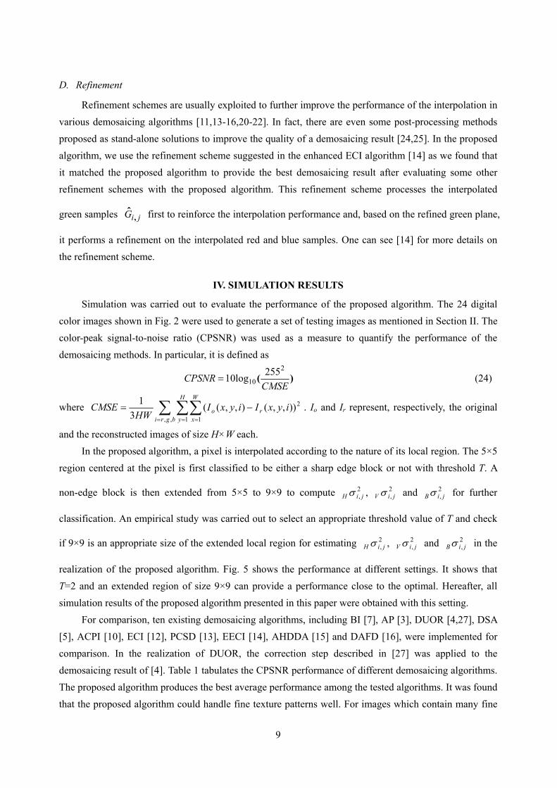
Fig. 6, 7 and 8 show some demosaicing results of images 1, 15 and 19 for comparison. They show that the proposed algorithm can preserve fine texture patterns and, accordingly, produce less color artifacts. Recall that the proposed algorithm is actually developed based on ACPI. As compared with ACPI, the proposed algorithm produces a demosaicing result of much less color artifact by interpolating missing components along a better direction. In fact, the average CPSNR of the proposed algorithm (39.93 dB) is much closer than that of ACPI (36.88 dB) to that achieved by the ideal ACPI (41.02 dB). These results show that the gradient test proposed in the proposed algorithm is more reliable than that of ACPI.

Table 2 shows the performance of various algorithms in terms of CIELab color difference [26]. The proposed algorithm provided the best performance among the evaluated algorithms again. With the proposed gradient testing tool, a simple heuristic algorithm can provide a subjectively and objectively better demosaicing performance as compared with many advanced algorithms [3-5,10,12-15].

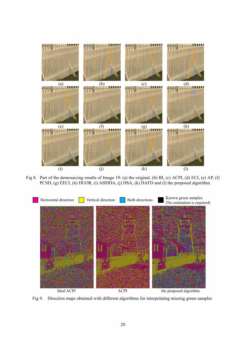
The proposed algorithm is developed based on the fact that the interpolation direction for each missing green sample is critical to the final demosaicing result. A study was carried out to investigate how significant the improvement with respect to ACPI could be when the proposed algorithm was used to find a better interpolation direction for a pixel. Note that demosaicing along edges in a natural image significantly reduces the demosaicing error. Fig. 9 shows some interpolation direction maps obtained with ACPI, the ideal ACPI and the proposed algorithm for comparison.

Table 3 shows the performance of ACPI and the proposed algorithm in finding an appropriate interpolation direction. This Table shows the contribution of 3 different groups of pixels to the MSE of the green plane in the final demosaicing result. Pixels in the testing images are grouped according to the following three constraints: (1) ACPID = iACPID ≠ oursD , (2) ACPID ≠ iACPID = oursD and (3)

ACPID ≠ iACPID ≠ oursD , where ACPID , iACPID and oursD are, respectively, a pixel’s interpolation

directions estimated with ACPI, the ideal ACPI and the proposed algorithm. One can see that the percentage of Group 2 pixels is higher than that of Group 1 pixels. This implies that, when the proposed algorithm is used, there are more hits on iACPID . Even in the case of iACPID ≠ oursD , the estimate of the

proposed algorithm is better in a way that the interpolation result provides a lower MSE. One can see the reduction in MSE/pixel achieved by the proposed algorithm in Group 3 pixels. Besides, the average penalty introduced by Group 1 pixels to the proposed algorithm is just 20.3(=28.8-8.5) while the average penalty introduced by Group 2 pixels to ACPI is 57.1(=64.3-7.2) in terms of MSE per pixel.

To a certain extent, the proposed algorithm is robust to the estimation result of 2, jiHσ , 2

, jiV σ and

2, jiBσ . In one of our simulations, for each (i,j), 2

, jiHσ , 2, jiV σ and 2

, jiBσ were separately corrupted by

11

adding a uniformly distributed random noise of range ±10% of their original estimated values to them. It was found that the final demosaicing results were more or less the same as the one without corruption in terms of both CIELab color difference and CPSNR.

Table 4 shows the complexity of the proposed algorithm. Note that some intermediate computation results can be reused during demosaicing and this was taken into account when the complexity of the

proposed algorithm was estimated. Its complexity can be reduced by simplifying the estimation of 2, jiHσ ,

2, jiV σ and 2

jiB ,σ . In particular, eqns. (11), (12) and (17) can be simplified by replacing Ψ with

},,{ 420 ±±=Ψs and turning all involved square operations into absolute value operations. Some

demosaicing performance is sacrificed due to the simplification. The simplified version provided an average CPSNR of 39.89 dB and an average CIELAB color difference of 1.6007 in our simulations. Its complexity is also shown in Table 4. In our simulations, the average execution times for the proposed algorithm and its simplified version to process an image on a 2.8GHz Pentium 4 PC with 512MB RAM are, respectively, 0.2091 s and 0.1945 s.

V. CONCLUSIONS

In this paper, an adaptive demosaicing algorithm was presented. It makes use of the color difference variance of the pixels located along the horizontal axis and that along the vertical axis in a local region to estimate the interpolation direction for interpolating the missing green samples. With such an arrangement, the interpolation direction can be estimated more accurately and, hence, more fine texture pattern details can be preserved in the output. Simulation results show that the proposed algorithm is able to produce a subjectively and objectively better demosaicing results as compared with a number of advanced algorithms.

VI. ACKNOWLEDGEMENT

This work was supported by a grant from the Research Grants Council of the Hong Kong Special Administrative Region, China (PolyU 5205/04E). The author would like to thank Dr. B. K. Gunturk at Lousisiana State University and Dr. X. Li at University of West Virginia for providing programs of their demosaicking algorithms [3,5].

VII. REFERENCES

[1] B. E. Bayer, “Color imaging array”, U.S. Patent 3 971 065, July 1976. [2] B. K. Gunturk, J. Glotzbach, Y. Altunbask, R. W. Schafer, and R. M. Mersereau, “Demosaicing:

color filter array interpolation”, IEEE Signal Processing Magazine, vol.22, no. 1, p.44-54, Jan. 2005. [3] B. K. Gunturk, Y. Altunbasak, and R. M. Mersereau, “Color plane interpolation using alternating

projections”, IEEE Trans. Image Processing, vol.11, no. 9, p.997-1013, Sept. 2002. [4] D. D. Muresan and T. W. Parks, “Demosaicing using optimal recovery”, IEEE Trans. Image

12

Processing, vol.14, no. 2, p.267-278, Feb. 2005. [5] X. Li, “Demosaicing by successive approximation”, IEEE Trans. Image Processing, vol.14, no. 3,

p.370-379, Mar. 2005. [6] D. Alleyson, S. Susstrunk and J. Herault, “Linear demosaicing inspired by human visual system”,

IEEE Trans. Image Processing, vol.14, no. 4, p.439-449, Apr. 2005. [7] T. Sakamoto, Chikako Nakanishi and Tomohiro Hase, “Software pixel interpolation for digital still

camera suitable for a 32-bit MCU”, IEEE Trans. Consumer Electronics, vol. 44, no. 4, p.1342-1352, Nov. 1998.

[8] D. R. Cok, “Signal processing method and apparatus for producing interpolated chrominance values in a sampled color image signal”, U.S. Patent 4 642 678, 1987.

[9] W. T. Freeman, “Median filter for reconstructing missing color samples”, U.S. Patent 4 724 395 1988.

[10] J. F. Hamilton and J. E. Adams, “Adaptive color plane interpolation in single sensor color electronic camera”, U.S. Patent 5 629 734, 1997.

[11] R. Lukac and K. N. Plataniotis, “Normalized color-ratio modeling for CFA interpolation”, IEEE Trans. Consumer Electronics, vol. 50, no. 2, p.737-745, May 2004.

[12] S. C. Pei and I. K. Tam, “Effective color interpolation in CCD color filter arrays using signal correlation”, IEEE Trans. Circuits and Systems for Video Technology, vol.13, no. 6, p.503-513, Jun. 2003.

[13] X. Wu and N. Zhang, “Primary-consistent soft-decision color demosaicing for digital cameras”, IEEE Trans. Image Processing, vol.13, no. 9, p.1263-1274, Sept. 2004.

[14] L. Chang and Y. P. Tam, “Effective use of spatial and spectral correlations for color filter array demosaicing”, IEEE Trans. Consumer Electronics, vol.50, no. 1, p.355-365, Feb. 2004.

[15] K. Hirakawa and T. W. Parks, “Adaptive homogeneity-directed demosaicing algorithm”, IEEE Trans. Image Processing, vol.14, no. 3, p.360-369, Mar. 2005.

[16] R. Lukac and K. N. Plataniotis, “Data-adaptive filters for demosaicking: A framework”, IEEE Trans. Consumer Electronics, vol. 51, no. 2, p.560-570, May 2005.

[17] R. Lukac and K. N. Plataniotis, ”Fast video demosaicking solution for mobile phone imaging applications”, IEEE Trans. Consumer Electronics, vol. 51, no. 2, p.675-681, May 2005.

[18] A. Lukin and D. Kubasov, “An improved demosaicing algorithm”, Graphicon, Moscow, Russia, Sept. 2004.

[19] R. Ramanath and W. E. Snyder, “Adaptive demosaicking”, Journal of Electronic Imaging, vol. 12, no. 4, p.633-642, Oct. 2003.

[20] W. Lu and Y. P. Tang, “Color filter array demosaicking: New method and performance measures”, IEEE Trans. Image Processing, vol.12, no. 10, pp.1194-1210, Oct. 2003.

[21] R. Lukac, K. N. Plataniotis, D. Hatzinakos and M. Aleksic, “A novel cost effective demosaicking approach”, IEEE Trans. Consumer Electronics, vol. 50, no. 1, p.256-261, Feb. 2004.

[22] N. Kehtarnavaz, H. J. Oh and Y. Yoo, “Color filter array interpolation using color correlations and

13

directional derivatives”, Electronic Imaging Journal, vol. 12, no. 4, p.621-632, Oct. 2003. [23] J. Adams, “Design of practical color filter array interpolation algorithms for digital cameras”, SPIE

Proceedings, vol. 3028, p.117-125, Feb.1997. [24] R. Lukac, K. Martin and K. N. Plataniotis, “Demosaicked image postprocessing using local color

ratios”, IEEE Trans. Circuits and Systems for Video Technology, vol.14, no. 6, p.914-920, Jun. 2004.

[25] R. Lukac and K. N. Plataniotis, “A robust, cost-effective postprocessor for enhancing demosaicked camera images”, Real-Time Imaging, SI on Spectral Imaging II, vol. 11, no. 2, p. 139-150, Apr. 2005.

[26] K. McLaren, “The development of the CIE 1976 (L*a*b*) uniform color-space and colour-difference formula”, Journal of the Society of Dyers and Colourists 92, pp. 338-341, 1976.

[27] D. D. Muresan and T. W. Parks, “Optimal recovery demosaicing”, IASTED Signal and Image Processing (Hawaii 2002).

14

Figure Captions

Fig. 1. Four 5×5 regions of Bayer CFA pattern having their centers at (a) red, (b) blue, (c)-(d) green CFA samples

Fig. 2. Set of testing images (Refers as image 1 to image 24, from top-to-bottom and left-to-right)

Fig. 3. An example where a simple gradient test does not work: (a) a 5×5 block in texture region, (b) pixel values along the vertical line across the block center and (c) pixel values along the horizontal line across the block center.

Fig. 4. A 9×9 window of Bayer CFA pattern

Fig. 5. Performance of the proposed algorithm at different settings of threshold T and window size

Fig. 6. Part of the demosaicing results of Image 1: (a) the original, (b) BI, (c) ACPI, (d) ECI, (e) AP, (f) PCSD, (g) EECI, (h) DUOR, (i) AHDDA, (j) DSA and (k) the proposed algorithm.

Fig. 7. Part of the demosaicing results of Image 15: (a) the original, (b) BI, (c) ACPI, (d) ECI, (e) AP, (f) PCSD, (g) EECI, (h) DUOR, (i) AHDDA, (j) DSA and (k) the proposed algorithm.

Fig. 8. Part of the demosaicing results of Image 19: (a) the original, (b) BI, (c) ACPI, (d) ECI, (e) AP, (f) PCSD, (g) EECI, (h) DUOR, (i) AHDDA, (j) DSA and (k) the proposed algorithm.

Fig. 9. Direction maps obtained with different algorithms for interpolating missing green samples.

Table Captions

Table 1. The CPSNR performance (in dB) of various algorithms

Table 2. Performance of various algorithms in terms of CIELAB color difference

Table 3. MSE contributed by different groups of pixels

Table 4. Arithmetic operations required by the proposed algorithm to estimate two missing color components at (a) a red/blue sampling position or (b) a green sampling position

15

j-2 j-1 j j+1 j+2 j-2 j-1 j j+1 j+2 j-2 j-1 j j+1 j+2 j-2 j-1 j j+1 j+2

i-2 R G R G R B G B G B G R G R G G B G B G

i-1 G B G B G G R G R G B G B G B R G R G R

i R G R G R B G B G B G R G R G G B G B G

i+1 G B G B G G R G R G B G B G B R G R G R

i+2 R G R G R B G B G B G R G R G G B G B G

(a) (b) (c) (d)

Fig 1. Four 5×5 regions of Bayer CFA pattern having their centers at (a) red, (b) blue, (c)-(d) green CFA samples

Fig 2. Set of testing images (Refers as image 1 to image 24, from top-to-bottom and left-to-right)

16

(a)

(b) (c)

Fig 3. An example where a simple gradient test does not work: (a) a 5×5 block in texture region, (b) pixel values along the vertical line across the block center and (c) pixel values along the horizontal line across the block center.

j-4 j-3 j-2 j-1 j j+1 j+2 j+3 j+4i-4 R i-3 G i-2 R i-1 G i R G R G R G R G R

i+1 G i+2 R i+3 G i+4 R

Fig 4. A 9×9 window of Bayer CFA pattern

0

50

100

150

200

250

1 2 3 4 5

Horizontal

B

G

R

0

50

100

150

200

250

1 2 3 4 5

Vertical B

G

R

17

39.0

39.1

39.2

39.3

39.4

39.5

39.6

39.7

39.8

39.9

40.0

0.5 1.0 1.5 2.0 2.5 3.0 3.5 4.0 4.5 5.0 5.5Threshold T

CPS

NR

5x59x913x13

(a) CPSNR

1.58

1.60

1.62

1.64

1.66

1.68

1.70

1.72

1.74

0.5 1.0 1.5 2.0 2.5 3.0 3.5 4.0 4.5 5.0 5.5Threshold T

∆-C

IELa

b

5x59x913x13

(b) CIELab color difference

Fig 5. Performance of the proposed algorithm at different settings of threshold T and window size

18

(a) (b) (c) (d)

(e) (f) (g) (h)

(i) (j) (k) (l)

Fig 6. Part of the demosaicing results of Image 1: (a) the original, (b) BI, (c) ACPI, (d) ECI, (e) AP, (f) PCSD, (g) EECI, (h) DUOR, (i) AHDDA, (j) DSA, (k) DAFD and (l) the proposed algorithm.

19

(a) (b) (c) (d)

(e) (f) (g) (h)

(i) (j) (k) (l)

Fig 7. Part of the demosaicing results of Image 15: (a) the original, (b) BI, (c) ACPI, (d) ECI, (e) AP, (f) PCSD, (g) EECI, (h) DUOR, (i) AHDDA, (j) DSA, (k) DAFD and (l) the proposed algorithm.

20

(a) (b) (c) (d)

(e) (f) (g) (h)

(i) (j) (k) (l)

Fig 8. Part of the demosaicing results of Image 19: (a) the original, (b) BI, (c) ACPI, (d) ECI, (e) AP, (f) PCSD, (g) EECI, (h) DUOR, (i) AHDDA, (j) DSA, (k) DAFD and (l) the proposed algorithm.

Ideal ACPI ACPI the proposed algorithm

Fig 9. Direction maps obtained with different algorithms for interpolating missing green samples

Vertical direction Both directions Horizontal direction Known green samples (No estimation is required)

21

Non-heuristic algorithms Heuristic algorithms

Image

AP [3]

DUOR [4,27]

DSA [5]

BI [7]

ACPI [10]

ECI [12]

PCSD [13]

DAFD [16]

EECI [14]

AHDDA [15]

Ours w/o refinement

Ours with refinement

Ideal ACPI

1 37.70 34.66 38.32 26.21 33.59 33.81 36.40 35.92 37.99 35.16 35.97 38.53 38.83 2 39.57 39.22 39.95 33.08 39.00 38.88 39.67 39.70 40.49 39.19 39.68 40.43 42.32 3 41.45 41.18 41.18 34.45 40.50 40.87 41.77 41.00 42.64 41.59 41.72 42.54 43.69 4 40.03 38.56 39.55 33.46 38.50 39.43 39.53 39.64 40.51 38.94 39.60 40.50 41.51 5 37.46 35.25 36.48 26.51 34.79 35.29 37.17 36.15 38.04 35.74 36.15 37.89 38.81 6 38.50 37.87 39.08 27.66 34.79 34.95 38.86 36.94 38.10 37.57 38.01 40.03 40.64 7 41.77 41.39 41.50 33.38 40.84 40.54 41.48 41.03 42.73 40.92 41.02 42.15 43.69 8 35.08 31.04 35.87 23.39 32.04 30.52 34.48 33.34 35.20 33.77 34.25 36.41 36.93 9 41.72 41.27 41.94 32.16 40.15 39.55 41.99 40.73 42.58 41.09 41.63 43.04 44.01

10 42.02 40.39 41.80 32.38 39.84 40.30 41.75 41.13 42.52 40.71 41.20 42.51 43.48 11 39.14 37.42 38.92 28.96 35.97 36.24 38.57 38.09 39.46 37.53 37.99 39.86 40.94 12 42.51 42.30 42.37 33.27 40.53 40.02 42.61 41.13 42.63 41.75 42.09 43.45 44.22 13 34.30 31.08 34.91 23.79 29.65 31.33 32.85 33.64 34.38 31.52 32.32 34.90 35.15 14 35.60 35.58 34.52 29.05 35.43 35.43 35.44 35.52 37.13 35.49 36.08 36.88 38.96 15 39.35 37.77 38.97 33.04 37.61 38.94 38.93 39.09 39.49 38.03 38.95 39.78 41.15 16 41.76 41.82 41.60 31.13 38.33 37.91 42.73 40.14 41.16 41.40 41.64 43.64 44.02 17 41.11 39.06 40.97 31.80 38.28 39.26 40.49 40.44 41.36 39.42 39.84 41.21 42.50 18 37.45 35.28 37.27 28.30 34.38 35.79 36.35 37.01 37.73 35.31 35.81 37.49 38.64 19 39.46 38.06 39.96 27.84 37.27 35.29 39.54 37.39 40.13 38.48 39.28 41.00 42.00 20 40.66 39.05 40.51 31.51 38.48 38.70 40.05 40.09 41.33 39.27 39.67 41.07 42.03 21 38.66 36.22 38.93 28.38 35.13 35.72 37.36 37.62 38.96 36.55 37.12 39.12 39.88 22 37.55 36.49 37.67 30.14 36.16 36.45 37.06 37.08 38.28 36.51 37.08 37.97 39.83 23 41.88 41.34 41.79 34.83 41.70 41.68 42.15 41.62 42.91 41.85 42.22 42.89 44.46 24 34.78 32.49 34.82 26.83 32.15 33.76 34.58 34.28 34.82 33.64 34.12 35.04 36.82

Avg. 39.15 37.70 39.12 30.06 36.88 37.11 38.83 38.28 39.61 37.98 38.48 39.93 41.02

Table 1. The CPSNR performance (in dB) of various algorithms

22

Non-heuristic algorithms Heuristic algorithms

Image

AP [3]

DUOR [4,27]

DSA [5]

BI [7]

ACPI [10]

ECI [12]

PCSD [13]

DAFD [16]

EECI [14]

AHDDA [15]

Ours w/o refinement

Ours with refinement

Ideal ACPI

1 2.1951 2.7929 2.0857 6.9234 3.1959 3.1093 2.3132 2.6083 2.0318 2.1596 2.4962 1.9593 1.8321 2 1.6534 1.6961 1.5998 2.7510 1.6841 1.7286 1.5883 1.6261 1.4975 1.6005 1.5849 1.4962 1.2211 3 1.0939 1.1618 1.1348 2.1091 1.2497 1.1894 1.0695 1.1579 0.9997 1.0488 1.1061 1.0121 0.8753 4 1.5918 1.8026 1.6831 2.8698 1.8506 1.6775 1.6654 1.6495 1.5132 1.6382 1.6509 1.5194 1.3317 5 2.1541 2.6927 2.3832 6.1880 2.7734 2.6353 2.1215 2.5646 1.9789 2.1745 2.3946 2.0273 1.8082 6 1.7629 1.7609 1.6761 5.1483 2.3906 2.4066 1.5949 2.0347 1.7369 1.5894 1.8065 1.5040 1.3980 7 1.2664 1.2981 1.3179 2.4452 1.3490 1.4015 1.2593 1.3798 1.1341 1.2712 1.3087 1.1935 1.0149 8 2.6797 3.5016 2.4892 8.5984 3.3803 4.0250 2.5900 3.1557 2.4474 2.4800 2.7809 2.2861 2.1051 9 1.2942 1.3418 1.2845 2.7976 1.4870 1.4849 1.2476 1.4124 1.2079 1.2655 1.2992 1.1749 1.0313

10 1.2686 1.4081 1.2808 2.7089 1.4832 1.4068 1.2614 1.3852 1.1941 1.2953 1.3233 1.2020 1.0523 11 1.6774 1.8338 1.6781 4.3695 2.1548 2.1592 1.6439 1.8283 1.5632 1.6188 1.7914 1.5230 1.3303 12 1.1438 1.1639 1.1586 2.4835 1.3577 1.3627 1.1153 1.2690 1.0998 1.1162 1.1827 1.0528 0.9476 13 3.0422 3.9801 2.8736 8.9385 4.8565 4.0087 3.4116 3.2657 2.9006 3.1335 3.6886 2.8559 2.6077 14 2.1081 2.2134 2.2754 4.6786 2.4424 2.3816 2.1065 2.2009 1.8860 2.0246 2.1468 1.9011 1.5915 15 1.4896 1.7072 1.5575 2.6978 1.7676 1.5655 1.5587 1.5607 1.4296 1.5615 1.5689 1.4306 1.2258 16 1.3657 1.2987 1.3491 3.6319 1.7686 1.8403 1.2310 1.5347 1.3694 1.2278 1.3746 1.1715 1.0930 17 1.3120 1.4781 1.3240 2.9295 1.6689 1.5384 1.3693 1.3853 1.2719 1.3612 1.4654 1.2938 1.1332 18 2.1519 2.5223 2.2502 4.8417 2.7406 2.3925 2.3095 2.2306 2.0536 2.2758 2.4023 2.1152 1.7496 19 1.7019 1.8779 1.6166 4.6739 2.0545 2.2889 1.6574 1.8830 1.5670 1.6290 1.7271 1.5029 1.3173 20 1.3160 1.4640 1.3288 2.6634 1.5736 1.5181 1.3626 1.3894 1.2311 1.3358 1.4135 1.2688 1.1254 21 1.7943 2.0671 1.7534 4.5763 2.4541 2.2627 1.9105 1.9516 1.6960 1.8171 2.0363 1.7029 1.5235 22 2.0209 2.2715 2.0630 3.9068 2.3258 2.1663 2.1026 2.0931 1.8905 2.1140 2.1364 1.9576 1.5651 23 1.1955 1.2727 1.2345 1.9242 1.2594 1.2185 1.2077 1.2206 1.1272 1.1917 1.2076 1.1429 0.9530 24 2.0345 2.4735 2.0804 4.8848 2.5768 2.3576 2.0625 2.2244 1.9014 2.0783 2.2044 1.9392 1.6510

Avg. 1.7214 1.9617 1.7283 4.1558 2.1602 2.0886 1.7400 1.8755 1.6137 1.7087 1.8374 1.5930 1.3952

Table 2. Performance of various algorithms in terms of CIELAB color difference

Group 1 Group 2 Group 3

Pixel nature of the group ACPID = iACPID ≠ oursD ACPID ≠ iACPID = oursD ACPID ≠ iACPID ≠ oursD

ACPI Ours w/o refinement ACPI Ours w/o

refinement ACPI Ours w/o refinement

% of pixels 17.12% 19.07% 34.84%

MSE/pixel 8.537 28.779 64.341 7.231 31.766 22.670

Table 3. MSE contributed by different groups of pixels

23

Original version Simplified version ADD MUL SHT CMP ADD MUL SHT CMP Edge/non-edge block classification 24 1 0 2 24 1 0 2 Estimating missing green sample

Case: edge block 9 0 5 0 9 0 5 0

Case: In non-edge block 95 39 11 2 59 4 7 2 Estimating missing red/blue sample 4 0 1 0 4 0 1 0 Refinement 19 14 0 0 19 14 0 0 Total

Case: edge block 56 15 6 2 56 15 6 2

Case: non-edge block 142 54 12 4 106 19 8 4

(a) Original version Simplified version ADD MUL SHT CMP ADD MUL SHT CMP

Estimating missing red sample 2 0 1 0 2 0 1 0 Estimating missing blue sample 2 0 1 0 2 0 1 0 Refinement 34 18 0 0 34 18 0 0

Total 38 18 2 0 38 18 2 0

(b)

Table 4. Arithmetic operations required by the proposed algorithm to estimate two missing color components at (a) a red/blue sampling position or (b) a green sampling position