
Collusion in Mixed Oligopolies and the Coordinated E ects ...wps.fep.up.pt/wps/wp590.pdf ·...
49
1,2 1,2 1 2
Transcript of Collusion in Mixed Oligopolies and the Coordinated E ects ...wps.fep.up.pt/wps/wp590.pdf ·...

n. 590 Jul 2017
ISSN: 0870-8541
Collusion in Mixed Oligopolies and the
Coordinated Eects of Privatization
João Correia da Silva1,2
Joana Pinho1,2
1 CEF.UP, Research Center in Economics and Finance, University of Porto2 FEP-UP, School of Economics and Management, University of Porto

Collusion in mixed oligopolies and the
coordinated effects of privatization
João Correia-da-Silva∗ and Joana Pinho†
July 5, 2017
Abstract: We study the sustainability of collusion in mixed oligopolies where private and public
firms only differ in their objective: private firms maximize profits, while public firms maximize
total surplus. If marginal costs are increasing, public firms do not supply the entire market,
leaving room for private firms to produce and possibly cooperate by restricting output. The
presence of public firms makes collusion among private firms harder to sustain, and maybe even
unprofitable. As the number of private firms increases, collusion may become easier or harder to
sustain. Privatization makes collusion easier to sustain, and is socially detrimental whenever firms
are able to collude after privatization (which is always the case if they are sufficiently patient).
Coordinated effects thus reverse the traditional result according to which privatization is socially
desirable if there are many firms in the industry.
Keywords: Collusion; Mixed oligopoly; Privatization; Coordinated effects.
JEL Codes: D43, H44, L13, L41.
We are grateful to Yassine Lefouili and two anonymous referees for extremely useful comments andsuggestions. Part of this work was developed while the two authors were at the Toulouse School ofEconomics. Joana Pinho acknowledges financial support from Fundação para a Ciência e a Tecnologia(FCT) through post-doctoral scholarship BPD/79535/2011. João Correia-da-Silva acknowledges financialsupport from the European Commission through Marie Curie fellowship H2020-MSCA-IF-2014-657283.This research was also financed by FEDER (COMPETE) and by Portuguese public funds (FCT), throughprojects PTDC/IIM-ECO/5294/2012 and PEst-OE/EGE/UI4105/2014.∗CEF.UP and Faculdade de Economia, Universidade do Porto. E-mail: [email protected]†Corresponding author. CEF.UP and Faculdade de Economia, Universidade do Porto. E-mail:
1

1 Introduction
All over the world, there are industries where private firms compete with public firms to
provide a good or service (OECD, 2005).1 Public and private firms are typically viewed
as pursuing different goals: private firms maximize profits, while public firms are to some
extent concerned about social welfare.2 Another virtue of public firms is that, while private
firms tend to engage in coordinated behavior that is mutually beneficial, public firms are
less likely to participate in collusive schemes.3
Our goal is to study the sustainability of collusion among private firms when facing
competition from public firms. Furthermore, we seek to understand how privatization
affects the incentives for private firms to collude and its ultimate impact on welfare.4 To
address these issues, we build a theoretical model where an arbitrary number of private
and public firms play an infinitely repeated game. In each period, firms simultaneously
choose quantities of a homogeneous good to sell in the market. We assume that marginal
production costs are increasing and that there is no cost asymmetry between public and
private firms.5 The only distinction between public and private firms is in their objective
1According to Barca and Becht (2001), in the middle 1990s, the number of non-financial companies controlledby the state was: 50 in Austria, 140 in Belgium, 372 in Germany, 193 in Spain, 214 in Italy, 137 in the Netherlands,304 in Sweden, and 207 in the UK. The presence of a public firm is most likely in sectors exhibiting market failureslike natural monopolies or public good provision. In mixed markets, a public firm may also constitute a regulatoryinstrument (Merrill and Schneider, 1966; Harris and Wiens, 1980; Cremer et al., 1989; Brandão and Castro, 2007).
2While Merrill and Schneider (1966) assumed that the objective of the public firm is to maximize total output,Harris and Wiens (1980) and De Fraja and Delbono (1989) assumed that the public firm maximizes total surplus.In more recent contributions, it is considered that public firms maximize a weighted sum of total surplus andown profit (Matsumura, 1998; Matsumura and Kanda, 2005; Colombo, 2016). Delbono and Lambertini (2016)assumed that the public firm maximizes a social welfare function wherein consumer surplus and own profits havemore weight than private firms’ profits.
3In 2013, four private firms that provided ferry transport services were fined by the Italian CompetitionAuthority for parallel price increases on the route between the mainland and Sardinia. These firms competedwith a public firm that was not found to be involved in the collusive agreement. For details, see ICA.I743-Tariffetraghetti da/per la Sardegna, Decision of 11 June 2013. In their empirical study on the Dutch waste collectionmarket, Dijkgraaf and Gradus (2007) also found evidence of collusion among private firms in the presence of publiccompetitors. These cases were brought to our attention by Colombo (2016).
4Usual motives pointed out by governments to support privatizations are: political reasons, the possibility ofmaking cash and increasing liquidity, and the inefficiency of public firms. See Starr (1988), Vickers and Yarrow(1991), and Megginson and Netter (2001), for deeper discussions on this topic.
5Public firms are sometimes considered to be less efficient than private firms (Cremer et al., 1989; Pal, 1998;George and La Manna, 1996; Matsumura and Shimizu, 2010). However, according to De Fraja and Delbono (1990,p. 9), “there does not seem to be enough empirical evidence to take this [relative] inefficiency for granted.”
2

function: private firms maximize profits, while public firms maximize total surplus.6 At the
beginning of the game, private firms may agree to produce, in each period, the quantities
that maximize their joint profit. To punish deviations from the collusive agreement, they
adopt grim trigger strategies, which consist of permanently reverting to the Cournot-Nash
equilibrium of the stage game after a deviation (Friedman, 1971).
We find that if the number of private firms is small or if the slope of the marginal
cost function is small, profits in the private sector are lower if private firms maximize
their joint profit than if they maximize individual profits. In this case, even if firms are
extremely patient, collusion is not sustainable. Collusion may reduce profits because an
output contraction in the private sector triggers an output expansion in the public sector
(due to strategic substitutability). Thus, collusion entails a negative strategic effect that
may overcome the positive direct effect of restricting output. This is the case if the number
of private firms is small, which means that the cartel fringe has a large market share; or
if the slope of the marginal cost function is small, which implies a large output expansion
by the public sector in reaction to collusion. This mechanism, through which coordination
entails a negative strategic effect that consists of an output expansion by outsiders, has
been explained by Salant et al. (1983) and Perry and Porter (1985) in their analysis of the
profitability of mergers among quantity-setting firms.7
Collusion is considered to be more likely in markets with a small number of firms (Motta,
2004; Ivaldi et al., 2007). By contrast, we find that, in mixed oligopolies, collusion may
become easier to sustain as the number of colluding firms increases.8 More precisely, when
there is a single public firm and few private firms (four or less), increasing the number of
private firms makes collusion easier to sustain (i.e., decreases the critical discount factor).9
Probably motivated by the waves of privatization observed around the world in the last
decades (OECD, 2005, pp. 22–23), a significant share of the literature on mixed oligopolies
has been concerned with the impact of privatization on welfare (e.g., Cremer et al., 1989;
De Fraja and Delbono, 1990; Nett, 1993; Anderson et al., 1997). However, most of the
6Our conclusions remain valid in the case in which a single public firm maximizes a weighted sum of totalsurplus and own profit (Section 5.1).
7The general finding that profit-maximization may reduce equilibrium profits is also a central feature of theliterature on strategic delegation (Fershtman and Judd, 1987; Sklivas, 1987).
8We recover the standard result in the benchmark case of private oligopolies (Appendix A).9The same conclusion holds when there are five or more private firms if the slope of the marginal cost function
is sufficiently small or sufficiently large.
3
existing literature does not take into account the possible impact of privatization on pri-
vate firms’ incentives to collude.10 Assuming non-cooperative behavior, De Fraja and
Delbono (1989) concluded that privatization is socially desirable if the number of firms is
sufficiently high. This is due to tendency of the public firm to produce a large output (to
increase consumer surplus), which makes private firms decrease their own output. When
the number of private firms is high, the concentration of production on the public firm
decreases productive efficiency to such an extent that total surplus becomes lower due to
the presence of a public firm.
We conclude that privatization always makes collusion among private firms easier to
sustain, and thus it may happen that collusion is not sustainable before privatization but
becomes sustainable afterward. If this is the case, there is an additional loss of total sur-
plus (the coordinated effects of privatization), which is the greater: the smaller is the slope
of the marginal cost function, and the greater is the number of private firms. To describe
the impact of privatization on total surplus, it is useful to distinguish three scenarios: (i)
collusion is not sustainable either before or after privatization; (ii) collusion is not sustain-
able before privatization but it is sustainable afterward; and (iii) collusion is sustainable
both before and after privatization. We find that privatization may only increase total
surplus in the first scenario, i.e., when firms behave non-cooperatively (De Fraja and Del-
bono, 1989). If private firms collude after privatization (regardless of whether they collude
or not before privatization), privatization is surely welfare detrimental.
Related literature
In most economic analyses of mixed oligopolies, it has been assumed that private firms
behave non-cooperatively. To the best of our knowledge, Merrill and Schneider (1966)
and Sertel (1988) were the first to consider that public firms may face competition from a
cartel of private firms.11 They used static models, which implicitly assume the existence of
an enforcement mechanism that prevents firms from cheating on the collusive agreement.
The recent contribution of Colombo (2016) is the closest to ours. He also built an
10Delbono and Lambertini (2016) showed that a credible threat of nationalizing a private firm may suffice toprevent collusion among private firms.
11To avoid the trivial outcome in which the public firm drives price down to marginal cost and thus elimi-nates any incentives to collude, Merrill and Schneider (1966) considered capacity constraints while Sertel (1988)considered cost asymmetries. In our model, a similar role is played by increasing marginal cost.
4

infinitely repeated game to study the impact of the presence of a public firm on the
sustainability of collusion among private firms. Nevertheless, there are important differ-
ences regarding the main goal, the basic setup and the policy implications. The pur-
pose of Colombo (2016) was to study the impact of the degree of public ownership of a
non-colluding firm on the sustainability of collusion; while we are primarily interested in
understanding the impact of the number of firms and of the slope of the marginal cost
function on the sustainability of collusion, as well as addressing the welfare impacts of
privatization when its potential coordinated effects are taken into account. In terms of
setup, Colombo (2016) assumed that the cartel behaves as a Stackelberg leader, while we
assume that the cartel and the public firm choose quantities simultaneously.12 Another
difference is that Colombo (2016) assumed that firms have constant marginal cost, while
we consider increasing marginal costs, as in De Fraja and Delbono (1989), among others.
Finally, Colombo (2016) considered that firms produce differentiated goods à la Singh and
Vives (1984), while we consider homogeneous goods.13
Colombo (2016) found that if goods are relatively close substitutes, the presence of
a public firm favors collusion between private firms. We obtain the opposite result. In
general, a firm produces more if it cares about total surplus than if it maximizes own
profit. As a result, the profits of colluding firms are lower when the non-colluding firm
is public. However, by lowering profits in all market regimes (collusion, deviation and
punishment), the presence of a public firm does not have a straightforward impact on the
sustainability of collusion: profits become lower along the collusive path (anti-collusive
effect) but the punishment becomes harsher and the deviation less tempting (pro-collusive
effects). Assuming that the cartel is a Stackelberg leader, Colombo (2016) found that
the pro-collusive effects outweigh the anti-collusive one. By contrast, assuming that the
cartel and the public firm choose quantities simultaneously, we conclude that the anti-
competitive effect dominates. This divergence suggests that authorities, when evaluating
the impact of public firms on the sustainability of collusion in the private sector, must
devote special attention to the order of moves of private and public firms.
In principle, Stackelberg leadership arises from the ability of a firm to commit to a
given choice of output. When multiple firms have commitment power, the appropriate
12Nevertheless, Colombo (2016) considered that, along the punishment phase, the leadership of the privatesector vanishes and, as in our model, private and public firms move simultaneously.
13It is product differentiation that, in his model, prevents the public firm from driving price down to marginalcost, independently of whether private firms collude or not. See Nett (1993).
5

timing can be established endogenously, by assuming that, in a prior stage, firms choose
whether to produce in the first or in the second period (Hamilton and Slutsky, 1990).
If firms choose the same period, there is Cournot competition; if they choose different
periods, there is Stackelberg leadership.14 In some contexts, public ownership (through
legislation) and cartelization (through the prevailing collusive agreement) may be plausible
sources of leadership.15 When commitment is not plausible, Cournot competition is the
most appropriate model.16
The remainder of the paper is organized as follows. Section 2 presents the model
and derives the optimal behavior of public and private firms. Section 3 analyzes the
sustainability of perfect collusion in mixed oligopolies. Section 4 studies the impact of
privatization on the sustainability of collusion and on total surplus. Section 5 shows that
our results remain qualitatively the same when the non-colluding firm is semi-public, and
when the cartel uses optimal penal codes. Section 6 concludes with some remarks.
14Considering competition between a semi-public firm and a private firm selling differentiated goods, Naya(2015) found that the equilibrium of this endogenous timing game crucially depends on the weight that the semi-public firm attaches to its own profits. More precisely, Naya (2015) found that: (i) if this weight is sufficientlyhigh, the semi-public and the private firm choose quantities simultaneously; (ii) for intermediate values of thisweight, the semi-public firm is the Stackelberg leader; (iii) if this weight is sufficiently small, the semi-public andthe private firm move sequentially and both firms may be the leader/follower. In the absence of collusion, Pal(1998) showed that, if the order of the moves is endogenous, public and private firms may not move simultaneously.More precisely, if firms support constant marginal costs but private firms are more efficient than the public firm,the public firm prefers to be a follower and produces no output. See also Matsumura (2003).
15According to George and La Manna (1996, p. 854), “the public firm can use its ownership status as a crediblecommitment. Being state-owned, in fact, means that the whole machinery of government regulation/legislationcan be deployed to make any commitment in terms of output (or price) irreversible and hence credible.” Colombo(2016, fn. 8) justified the assumption of the cartel being a Stackelberg leader on the grounds that “the collusivequantity is a less flexible decision than the quantity set autonomously by the non-colluding firm.”
16As De Fraja and Delbono (1990) pointed out in their survey, there are contributions considering that thepublic firm is a Stackelberg leader (Sertel, 1988; De Fraja and Delbono, 1989; George and La Manna, 1996; Fjelland Heywood, 2004), a Stackelberg follower (Beato and Mas-Colell, 1984; Colombo, 2016), and that the public firmmoves simultaneously with private rivals (Cremer et al., 1989; Matsumura, 1998; Matsumura and Kanda, 2005;Delbono and Lambertini, 2016). This diversity extends to the empirical literature. Magnus and Midttun (2000)found empirical evidence that the public Norwegian supplier of electricity behaves as a follower with respect toprivate firms. By contrast, in their study on the health care industry, Barros and Martinez-Giralt (2002) assumedthat the public firm chooses price and quality before the private firm. Finally, the European automobile andairline industries, which are typical examples of mixed oligopolies, are treated in the empirical literature underthe assumption of Cournot competition (Matsushima and Matsumura, 2006).
6

2 Basic setting
Consider an industry with np ≥ 2 private firms and ng ≥ 0 public firms that produce
homogeneous goods and interact in an infinite number of periods.17 In each period, firms
simultaneously choose quantities to sell in the market. Inverse demand in period t ∈0, 1, ... is given by pt = 1−Qt, where Qt is the total output.
We assume that marginal production costs are increasing in output18 and, for simplicity,
that there is no cost asymmetry between public and private firms.19 Precisely, we assume
that the total cost of producing q ≥ 0 units of output is:
C(q) =α
2q2 + βq, with α ≥ 0 and 0 ≤ β < 1.
The only difference between public and private firms is in their objective functions.20 A
private firm i ∈ Ip maximizes the discounted flow of its profits, given by∑+∞
t=0 δtπit, where
δ ∈ (0, 1) denotes the discount factor and πit is the profit in period t. By contrast, a public
firm j ∈ Ig seeks to maximize the discounted sum of total surplus,∑+∞
t=0 δtTSt, where TSt
denotes total surplus in period t.
Public firms behave non-cooperatively, simultaneously choosing their output with the
objective of maximizing total surplus (TS), given by the sum of private firms’ profits,
17It is frequent to assume the existence of a single public firm (e.g., Pal, 1998; De Fraja and Delbono, 1989;Matsumura and Kanda, 2005; Colombo, 2016). However, as pointed out by Matsumura and Shimizu (2010), thereare several examples of real markets where more than one public firm is active, namely in banking, energy andtransportation sectors. Haraguchi and Matsumura (2016) have also considered multiple public firms.
18As explained by De Fraja and Delbono (1989, p. 303), with constant marginal cost, the public firm wouldprice at the marginal cost and supply the difference between demand and private firms’ output. Nett (1993) alsocame to this conclusion and called it the “Cournot paradox” in a mixed market. In this case, collusion betweenprivate firms would have no impact on total output and price, and would thus surely be unprofitable.
19 This additional source of asymmetry between public and private firms could obscure our results. Furthermore,according to De Fraja and Delbono (1990), there is not sufficient empirical evidence supporting the inefficiencyof public firms relatively to private firms. Nevertheless, there are several contributions in the literature assumingthat public firms and private firms have asymmetric costs. See, for example, Matsumura and Shimizu (2010)(quadratic production costs) and Haraguchi and Matsumura (2016) (linear production costs).
20Our basic setting is similar to that adopted by De Fraja and Delbono (1989). The main difference is that weassume coordination among private firms, while they assumed non-cooperative behavior.
7

public firms’ profits, and consumer surplus (CS):21
TS =∑
i∈Ipπi +
∑
j∈Igπj + CS = (1− β −Q)Q− α
2
(∑
i∈Ipq2i +
∑
j∈Igq2j
)+Q2
2. (1)
Taking as given the quantities produced by the other firms, a public firm j ∈ Ig chooses
the level of output qj that maximizes total surplus. Adding the best-reply functions of the
ng public firms, we obtain the reply function of the public sector:
Qg =ng
ng + α(1− β −Qp) , (2)
where Qp =∑
i∈Ip qi and Qg =∑
j∈Ig qj denote the total output produced by private firms
and public firms, respectively.
If the private sector restricts production, the public sector reacts by expanding pro-
duction. As marginal production costs are increasing in output, this compensation is only
partial. More precisely, if the private sector reduces production by one unit, the public
sector increases production by ngng+α
units. The greater is the slope of the marginal cost
function, the less responsive is the public sector, because expanding output has a greater
impact on marginal cost.
The output of each public firm, qg, is such that its marginal cost equals the market
price; while the output of each private firm, qp, is such that its marginal cost equals
marginal revenue (individual marginal revenue in the case of non-cooperative behavior;
private sector marginal revenue in the case of collusive behavior), which is lower than the
market price. Therefore, each private firm produces less than each public firm, and thus
private firms exhibit lower marginal cost than public firms.22
21As demand and costs are stationary, we slightly abuse notation by omitting subscripts t henceforward.22This underlies the finding of Matsumura (1998) that having a semi-public firm (which maximizes a weighted
sum of total surplus and own profits) is socially preferable to having a public firm (which maximizes total surplus).
8

3 Collusion
At the beginning of the game, private firms seek to establish an all-inclusive agreement
to produce the quantities that maximize their joint profit. To punish deviations from
the agreement, firms adopt grim trigger strategies, according to which they permanently
revert to Cournot competition after a deviation (Friedman, 1971).
In Appendix B, we obtain the profit of a private firm: under collusion, πmp ; under
competition, πcp; and in the case of a unilateral deviation, πdp .
3.1 Profitability of collusion
If the profit of private firms is lower under collusion than under competition (πmp < πcp),
collusion is surely not sustainable, because firms prefer to be punished rather than to
comply with the collusive agreement.
Proposition 1. Profits in the private sector are lower under collusion than under com-
petition if and only if the number of private firms is sufficiently small:
πmp < πcp if and only if np < n∗p(α, ng),
where:
n∗p(α, ng) ≡ng + α
4α2
[2ng + α(2 + ng)− α2 +
√(2 + α)2
(n2g + α2
)+ 2αng (4− α2)
]. (3)
Equivalently, collusive profits are lower than non-cooperative profits if and only if the slope
of the marginal cost function is sufficiently small: πmp < πcp if and only if α < α∗(np, ng),
where α∗(np, ng) is implicitly defined by n∗p(α, ng) = np.
Proof. See Appendix C.
As illustrated in Figure 1, if there are few private firms in the market, perfect collusion is
9

Πpm
< Πpc
Πpm
> Πpc
2 3 4 5 6 7 8 9 10np
0.5
1
1.5
2
2.5
2.7
Α
Figure 1. Comparison of private firms’ profits undercollusion and competition (ng = 1).
not profitable (and, of course, not sustainable). This result is specific to mixed oligopolies,
since replacing ng = 0 in (3), we obtain n∗p(α, 0) = 1.
When the private sector restricts output, the public sector reacts by expanding output
(Figure 2). As a result, the residual demand of the private sector is lower under collusion
than under competition. Therefore, when deciding whether or not to collude, private
firms face the following trade-off: on the one hand (taking as given the output of the
public sector), restricting output allows them to increase price and profits; on the other
hand (due to the adverse reaction by the public sector), restricting output reduces their
residual demand. In a private oligopoly where the collusive agreement is all-inclusive, the
adverse effect does not exist and, as a result, profits are surely higher under collusion. In
mixed markets where only private firms collude, the number of cartel members is crucial
to determine which of these two effects dominates. If np is small, since the intensity of
competition is low, the gains from cooperation are insufficient to compensate the output
expansion by the public firm in response to collusion in the private sector.23 If np is
large, private firms compete fiercely, and, therefore, the gains from cooperation more than
compensate the demand reduction that is due to the reaction of the public sector.
23This result is closely related to the unprofitability of mergers between quantity-setting firms when the mergerinvolves a small number of firms in the market (Salant et al., 1983; Perry and Porter, 1985).
10

QgHQpLQpc HQgLQp
mHQgL
0 Qpm Qp
c 1Qp
Qgc
Qgm
1
Qg
0 1-Qgm 1-Qg
c 1Qp
1-Qgc
1-Qgm
1
PHQpL
Figure 2. Output expansion in the public sector when the private sector changes from a cooperative toa non-cooperative behavior (α = 0.5, β = 0, np = 5, ng = 1).
The slope of the marginal cost function determines how much the residual demand of
the private sector shrinks due to the public sector’s reaction to collusion. If marginal cost
does not increase much in output, it is not very costly for the public sector to expand
output, and thus its reaction to collusion is very aggressive. In that case, private firms
prefer to compete rather than to collude.
3.2 Sustainability of collusion
Perfect collusion in the private sector is sustainable as a subgame perfect Nash equilibrium
if and only if the discounted flow of the profits of a private firm if it abides by the collusive
agreement is greater than its discounted flow of profits if it deviates, i.e., if and only if the
following incentive compatibility constraint (ICC) is satisfied:
+∞∑
t=0
δtπmp ≥ πdp ++∞∑
t=1
δtπcp ⇔ δ ≥ πdp − πmpπdp − πcp
. (4)
From Proposition 1, if np < n∗p, the critical discount factor is greater than 1, which means
that collusion cannot possibly be sustained. If np > n∗p, collusion is sustainable as long as
11
firms are sufficiently patient.
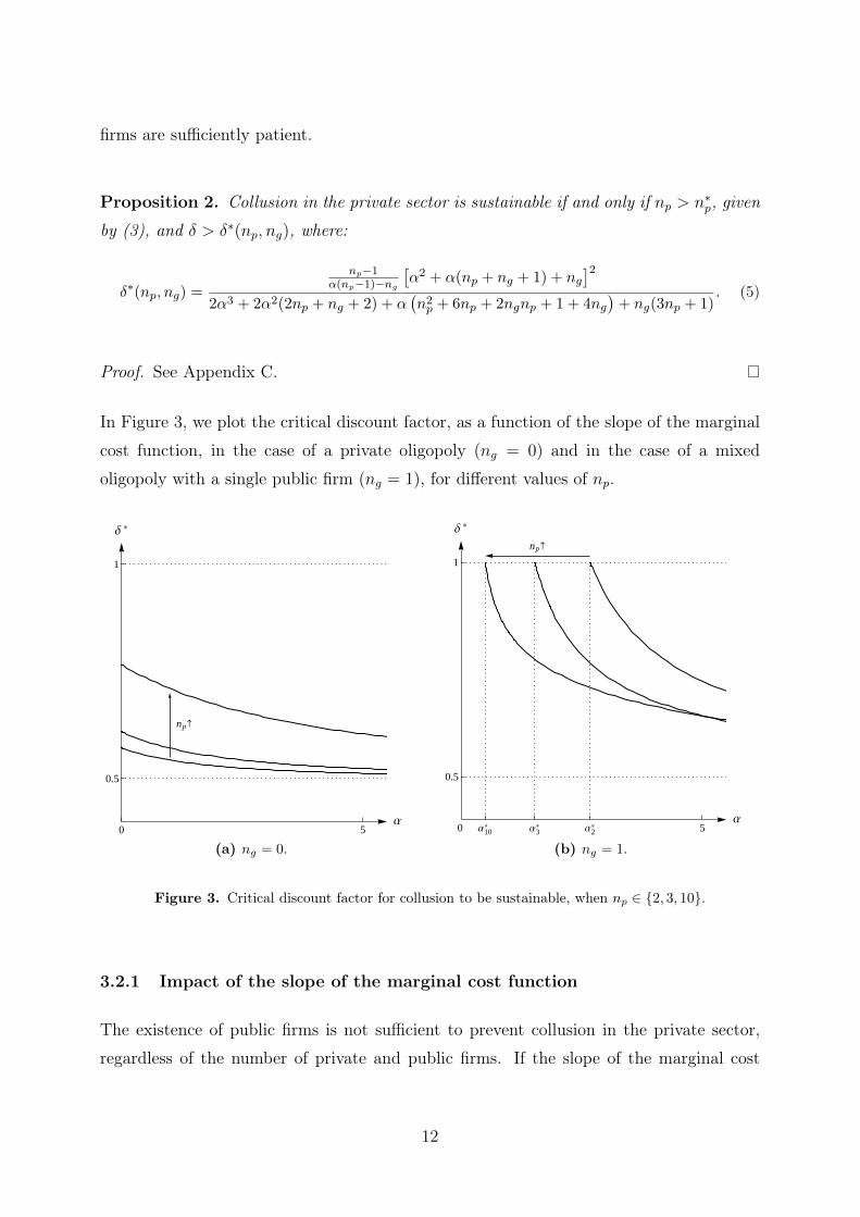
Proposition 2. Collusion in the private sector is sustainable if and only if np > n∗p, given
by (3), and δ > δ∗(np, ng), where:
δ∗(np, ng) =
np−1α(np−1)−ng
[α2 + α(np + ng + 1) + ng
]2
2α3 + 2α2(2np + ng + 2) + α(n2p + 6np + 2ngnp + 1 + 4ng
)+ ng(3np + 1)
. (5)
Proof. See Appendix C.
In Figure 3, we plot the critical discount factor, as a function of the slope of the marginal
cost function, in the case of a private oligopoly (ng = 0) and in the case of a mixed
oligopoly with a single public firm (ng = 1), for different values of np.
np
0 5Α
0.5
1
∆ *
(a) ng = 0.
np
0 Α2*Α3
*Α10* 5
Α
0.5
1
∆ *
(b) ng = 1.
Figure 3. Critical discount factor for collusion to be sustainable, when np ∈ 2, 3, 10.
3.2.1 Impact of the slope of the marginal cost function
The existence of public firms is not sufficient to prevent collusion in the private sector,
regardless of the number of private and public firms. If the slope of the marginal cost
12

function is sufficiently high (more precisely, if α > α∗) and firms are sufficiently patient,
collusion is sustainable. Notice also that:
limα→+∞
δ∗(np, ng) =1
2, ∀(np, ng).
Since marginal costs are increasing, it is not socially desirable to have public firms pro-
ducing too much output, and this is what leaves room for private firms to collude.
Proposition 3. In a mixed oligopoly, the greater is the slope of the marginal cost function,
the easier it is to sustain collusion, i.e., ∂δ∗∂α
< 0.
Proof. See Appendix C.
This result also holds in a private oligopoly (see Appendix A). Increasing marginal costs
make it more costly to expand output, reducing the relative gain from deviating unilater-
ally. As a result, collusion becomes easier to sustain.
3.2.2 Impact of the number of private firms
In private oligopolies, an increase in the number of firms makes it harder to sustain an
all-inclusive collusive agreement (Motta, 2004; Ivaldi et al., 2007).24 But if the collusive
agreement is partially inclusive, an increase in the number of firms in the cartel may
be expected to foster collusion sustainability by making collusion more profitable (Salant
et al., 1983; Perry and Porter, 1985).25
In mixed oligopolies, by contrast, the critical discount factor for collusion to be sus-
tainable does not vary monotonically with the number of firms in the cartel.
Proposition 4. Consider a mixed oligopoly with a single public firm, ng = 1 and assume
that condition (3) is satisfied, i.e., that collusion is profitable.
24This is true in our setting when all firms are private (ng = 0). See Proposition 11 in Appendix A.25It is important to note that the dynamics of entry originate effects on collusion sustainability that are not
captured in comparative statics on the number of firms. See ?, ? and the references therein.
13

(a) If np ≤ 4, increasing the number of private firms makes it easier to sustain collusion:
δ∗(2, 1) > δ∗(3, 1) > δ∗(4, 1) > δ∗(5, 1).
(b) If np ≥ 5 and the slope of the marginal cost function is sufficiently small or sufficiently
large, increasing the number of private firms makes collusion easier to sustain; but the
opposite occurs if the slope is intermediate (Figure 4).
Proof. See Appendix C.
A
B C
2 3 4 5 6 7 8np
lnH0.1L
lnH2.7L
lnH10L
lnHΑ L
[A] πmp < πc
p
[B] δ∗(np + 1, 1) < δ∗(np, 1)
[C] δ∗(np + 1, 1) > δ∗(np, 1)
Figure 4. Impact of np on δ∗(np, 1).
To understand this result, start by recalling that a change in the output of the public
sector shifts the demand of the private sector. We can relate the profit of a private firm
in the presence and in the absence of a public sector:
πkp(np, ng) = πkp(np, 0)
[1− β −Qk
g(np, ng)
1− β
]2
, (6)
where πkp denotes the profit of a private firm in market regime k ∈ m, d, c; and Qkg
denotes the corresponding public output level (Qdg = Qm
g > Qcg).
14

From the perspective of private firms, an output expansion by the public sector is akin
to a decrease of the market reservation price or an increase of the constant term of the
marginal production cost (β). If the public sector expands (resp. restricts) production,
the residual market faced by private firms shrinks (resp. expands).
Replacing expressions (6) in the ICC (4), we can write the critical discount factor for
collusion to be sustainable in a mixed oligopoly as function of profits in a private oligopoly,
πkp(np, 0), and of the output level of the public sector:
δ∗(np, ng) =πdp(np, 0)− πmp (np, 0)
πdp(np, 0)− πcp(np, 0)ρ(np, ng), (7)
where ρ(np, ng) ≡[
1−β−Qcg(np,ng)
1−β−Qmg (np,ng)
]2
> 1 is the ratio between market profitability when
the public firm produces Qcg relatively to when it produces Qm
g . This ratio describes the
increase of non-cooperative profits relatively to collusive and deviation profits that results
from the output contraction by the public firm, in response to the cartel breakdown.
If the residual demand of the private sector had the same size regardless of whether
the firms were cooperating or not (i.e., if ρ = 1), the expression for the critical discount
factor in a mixed oligopoly would be exactly the same as in a private oligopoly. In that
case: an increase in the number of cartel members would make collusion less sustainable
(see Appendix A). But the residual demand of private firms is smaller when they collude
(ρ > 1), and this reverses the previous conclusion if np ≤ 4 or if the slope of the marginal
cost function is sufficiently small or sufficiently large.
An increase in the number of private firms, np, has two effects: it increases the number
of private (colluding) firms; and it increases the fraction of private (colluding) firms in the
industry, npnp+ng
. If the number of private firms is small, the effect that seems to dominate
is the pro-collusive effect of the relative decrease of the size of the cartel fringe. If the
number of private firms is large, the importance of the cartel fringe is minor, and the
effect that seems to dominate is the anti-collusive effect of the increase in the number
of colluding firms. Figure 5 shows that non-monotonicity of the critical discount factor
as a function of the number of private firms does not totally disappear if we keep the
ratio between public and private firms fixed as we increase np.26 But the region in which
sustainability of collusion is enhanced by entry becomes significantly smaller.
26To keep this ratio fixed, we pay the price of allowing non-integer numbers of firms.
15

k=0.2
k=0.4
k=0.6
2 3 4 5 6 7 8 9 10np0.5
0.6
0.7
0.8
0.9
1
δ*(np, knp)
Figure 5. Critical discount factor as a function of the numberof firms for different values of k ≡ ng
np(with α = 3).
4 Coordinated effects of privatization
Two opposite effects of privatization on social welfare are recognized in the literature.
On the one hand, privatization reduces of total output, which increases the dead-weight
loss of welfare (as total output is below the first-best level). This cost of privatization
is the smaller the higher the number of private firms (as total output is closer to the
first-best level). On the other hand, privatization increases production efficiency. As
marginal production costs are increasing, private firms have lower marginal production
costs than public firms (since they produce less output). As a result, privatization leads
to a reallocation of production towards firms with lower marginal costs.27 This benefit
of privatization is the larger the greater is the number of private firms (as the output
asymmetry between public and private firms is larger). Privatization is socially desirable
whenever the production efficiency effect dominates the total production effect, which is
the case if the number of firms in the market is sufficiently high (De Fraja and Delbono,
1989; Matsumura and Shimizu, 2010; Matsumura and Okamura, 2015).
Existing contributions neglect that privatization affects the incentives for private firms
27Matsumura and Shimizu (2010) pointed out that, when there are several public firms in the market, privati-zation leads to a reallocation of production from the privatized firm to private firms (which increases total surplus)but also to the other public firms (which decreases total surplus).
16

to collude. We contribute to the discussion of the welfare impacts of privatization when
coordinated effects are taken into account.
To simplify the exposition, we assume that there is a single public firm (ng = 1) before
the privatization.28 Privatization thus changes the market from a mixed oligopoly with npprivate firms and a single public firm to a private oligopoly with np + 1 firms.29
Proposition 5. Collusion is easier to sustain in a private oligopoly with np+1 firms than
in a mixed oligopoly with np private firms and one public firm:
δ∗(np + 1, 0) < δ∗(np, 1).
Proof. See Appendix C.
∆*H2,1L
∆*H3,0L
A
BC
0 Α2* 10
Α
4
7
1
∆
(a) np = 2.
∆*H9,1L
∆*H10,0L
A
B C
0 Α9* 10
Α
121
161
1
∆
(b) np = 9.
[A] Collusion is not sustainable neither before nor after the privatization.[B] Collusion is sustainable after the privatization but not before.[C] Collusion is sustainable before and after the privatization.
Figure 6. Impact of privatization on the sustainability of collusion.
28For an analysis of privatization in markets with more than one public firm, see Matsumura and Shimizu(2010). These authors studied the welfare impacts of sequential privatizations and concluded that, if the number offirms is sufficiently high, the impact of privatization on social welfare varies non-monotonically with the number ofprivatized firms. Matsumura and Shimizu (2010) did not take into account the coordinated effects of privatization.
29For a study on partial privatization, see Matsumura (1998). Lin and Matsumura (2012) characterized theoptimal degree of privatization when a fraction of the partially privatized firm is owned by foreign investors.
17

If privatization makes collusion sustainable (region B in Figure 6), then it generates an ad-
ditional welfare loss, Ω(np), which results from the transition from competition to collusion
among private firms:
Ω(np) = TSc(np + 1, 0)− TSm(np + 1, 0), (8)
where TSc(np + 1, 0) and TSm(np + 1, 0) denote total surplus in a private oligopoly when
the np + 1 private firms compete and when they collude, respectively.
Proposition 6. Suppose that collusion is not sustainable before privatization but it is
sustainable afterward, i.e., that δ∗(np + 1, 0) < δ < δ∗(np, 1). The welfare loss associated
with cartelization is strictly positive, decreases with the slope of the marginal cost function,
and increases with the number of private firms:
Ω(np) > 0,∂Ω
∂α< 0 and Ω(np + 1) > Ω(np).
Proof. See Appendix C.
This welfare loss mitigates the result obtained by De Fraja and Delbono (1989), who as-
serted that when there are many private firms in the market, regulation is not as necessary,
because competition is more intense. Actually, the greater is the number of private firms,
the greater is the output restriction that results from their coordination, and, therefore,
the greater is the welfare loss associated with cartelization.
The following result describes the impact of privatization on total surplus.
Proposition 7. The impact of privatization on total surplus depends on the market regime
that prevails after privatization. Precisely:
(a) If collusion is sustainable after privatization, privatization decreases total surplus.
This implies that privatization decreases total surplus if firms are sufficiently patient.
(b) If collusion is not sustainable after privatization, privatization increases total surplus
18

if and only if the number of private firms is sufficiently high (Figure 7):
np >1
2
[√(1 + 2α) (4 + 5α + 2α2)
α− 1
]. (9)
Proof. See Appendix C.
TS
TS¯
2 3 4 5np
0.5
1
1.5
2
Α
Figure 7. Impact of privatization on total surplus, whencollusion is not sustainable after privatization.
If collusion is not sustainable after privatization, it is surely not sustainable before pri-
vatization (Proposition 5). In this case, we corroborate the result obtained by De Fraja
and Delbono (1989), regarding the potential desirability of privatization. Notice, however,
that this is the only scenario wherein privatization may improve welfare.30 If private firms
are able to collude after privatization (regardless of whether or not they are able to collude
before privatization), privatization is surely detrimental to total surplus.31
30Still, it never does if there are initially two private firms and one public firm (Corollary 2 in Appendix C).31Matsumura (1998) found that, when public and private firms have the same cost structure, neither full
privatization nor full nationalization are socially optimal. A semi-public firm that maximizes a weighted sum ofsocial welfare and profits is found to generate a higher total surplus. By contrast, Matsumura and Kanda (2005)found that if there is free entry of private firms, total surplus is the highest if the public firm maximizes totalsurplus. Their conclusion stems from the fact that a more aggressive behavior by the public firm hinders wastefulentry of private firms.
19

5 Extensions
5.1 Semi-public firm
In the literature on mixed oligopolies, it is frequently assumed that public firms maximize a
weighted average of total surplus and own profit (Bös, 1987; Matsumura, 1998; Matsumura
and Kanda, 2005; Colombo, 2016). This objective function may reflect joint ownership by
the state and by private shareholders. But even if a public firm is totally owned by the
state, assuming that it maximizes total surplus implicitly presumes that the government
is benevolent and perfectly controls managers’ actions. However, this may not be the
case and the objectives of the managers of public firms may differ from total surplus
maximization (De Fraja and Delbono, 1990; Barros, 1995).
We now check the robustness of our main results when the public firm, s, maximizes a
weighted sum of total surplus (TS) and own profit (πs):32
θTS + (1− θ)πs, with θ ∈ [0, 1]. (10)
Proposition 8. In the presence of a semi-public firm, collusion between private firms
is profitable if and only if the number of private firms is sufficiently small. A profitable
collusive agreement is sustainable if and only if:
δ >(np − 1) [(np + 1 + α)(1− θ + α) + 1 + α]2
[(np − 1)(1− θ + α)− 1][n2p(1 + α− θ) + np(3 + 2α)(3 + 2α− 2θ) + (1 + 4α + 2α2) (2 + α− θ)
] .
(11)
Proof. See Appendix C.
As illustrated in Figure 8, the more weight the semi-public firm attaches to total surplus
(i.e., the higher is θ), the larger is the region of parameters for which collusion in the
private sector is unprofitable.
32Multiple semi-public firms would complicate the analysis without qualitatively changing the results.
20

Πpm
> Πpc
Πpm
< Πpc
Θ =0.5
Θ =1
Θ =0
2 3 4 5 6 7 8np
0.5
1
1.5
2
2.5
2.7
Α
Figure 8. Comparison between collusive and competitive profitsof private firms, in the presence of a semi-public firm.
Corollary 1. The more the semi-public firm weights total surplus, the more difficult it is
to sustain collusion in the private sector.
Proof. See Appendix C.
Start by noticing that the higher is the weight the semi-public firm attaches to total
surplus, the more responsive is the semi-public firm to changes in the output of the private
sector, since ∆Qs∆Qp
= − 12−θ+α . Thus, a higher θ has two countervailing effects on the
sustainability of collusion. On the one hand, a higher θ implies that the semi-public firm
increases its output more when the private sector restricts output due to collusion, which,
by lowering collusive profits, hinders collusion. On the other hand, the higher is θ, the
lower are the punishment and deviation profits, which, by harshening the punishment and
making the deviation less profitable, facilitate collusion. Colombo (2016) found that if
the cartel behaves as a Stackelberg leader along the collusive path, the pro-collusive effect
dominates, i.e., a higher value of θ facilitates collusion among private firms. By contrast,
21

we obtain that, when the cartel and the semi-public firm move simultaneously, a higher
value of θ hinders collusion.
Figure 9 illustrates the impact of an additional private firm on the critical discount
factor. If np ≤ 4, regardless of the weight that the semi-public firm attaches to total
surplus, increasing the number of private firms makes collusion easier to sustain. The
higher is θ, the larger is the parameter region for which increasing the number of private
firms makes collusion easier to sustain (Appendix C).
Θ =0 Θ =0.25
Θ =0.5
Θ =1
2 3 4 5 6 7 8 9 10 11 12 13 14np
lnH0.01L
lnH0.1L
lnH10L
lnH100L
lnHΑ L
Figure 9. Condition δ?(np + 1, 1) = δ?(np, 1) for different values of θ. To theright of the plotted curves, entry hinders collusion, i.e., δ?(np + 1, 1) > δ?(np, 1).
Proposition 9. The welfare impact of the privatization of the semi-public firm depends
on the market regime that prevails after privatization:
(a) If collusion is sustainable after privatization, privatization decreases total surplus.
This implies that privatization decreases total surplus if firms are sufficiently patient.
(b) If collusion is not sustainable after privatization, privatization increases total surplus
if and only if the number of private firms is sufficiently large.
Proof. See Appendix C.
22

Θ =0.25Θ =0.5Θ =1
5 10 15 20np
1
2
Α
Figure 10. Impact of privatization on total surplus (it ispositive to the right of the plotted curves).
The threshold number of private firms above which privatization is socially beneficial is
plotted in Figure 10, when collusion is not sustainable neither before nor after privatization.
The less the semi-public firm weights total surplus (i.e., the lower is θ), the more likely it
is that privatization generates a loss of total surplus.
5.2 Optimal punishment strategies
Until now, we have assumed permanent reversion to the Cournot-Nash equilibrium of the
stage game after a deviation from the collusive agreement. As explained by Abreu (1986),
firms can adopt harsher punishments to reduce the continuation payoff after a deviation
and thus make the collusive agreement easier to sustain.
We now characterize the harshest symmetric punishment that firms may inflict, focusing
on stick-and-carrot strategies according to which, after a deviation, there is one period of
severe punishment followed by permanent reversion to the collusive outcome if all firms
have complied with the punishment (otherwise, the punishment is restarted).
For collusion to be sustainable, the punishment must be sufficiently harsh and must
also be credible. It is necessary that firms have incentives to: (i) comply with the collusive
agreement rather than deviate; (ii) execute the punishment rather than deviate.
23

Firms have incentives to comply with the collusive agreement if and only if:
+∞∑
t=0
δtπmp ≥ πdp + δ
(πpp +
+∞∑
t=1
δtπmp
)⇔ δ ≥ πdp − πmp
πmp − πpp, (12)
where πpp denotes the profit of a private firm in the punishment period.
Firms have incentives to execute the punishment if and only if:
πpp + δ+∞∑
t=0
δtπmp ≥ πdpp + δ
(πpp + δ
+∞∑
t=0
δtπmp
)⇔ δ ≥ πdpp − πpp
πmp − πpp, (13)
where πdpp denotes the profit of a firm that unilaterally deviates in the punishment period.
For simplicity, we set ng = 1 and α = 3, and we restrict the analysis to np ≤ 14. With
ng > 1 and α 6= 3, we would obtain longer mathematical expressions but we believe that
the results would qualitatively remain the same. For np ≥ 15, the public firm would shut
down in the punishment period, and thus analytical expressions would change.
Proposition 10. Let ng = 1, np ≤ 14 and α = 3. If firms adopt optimal punishments
strategies, collusion in the private sector is sustainable if and only if δ ≥ δop(np), where:
δop(np) =(np − 1) (3np + 16)2
20 (3np − 4) (7np + 12). (14)
Proof. See Appendix C.
Figure 11 compares the critical discount factor for collusion sustainability when firms adopt
optimal punishments and when they adopt grim trigger strategies. Notice that the impact
of the number of firms on the critical discount factor is qualitatively the same regardless of
whether firms adopt trigger strategies or optimal punishments, and that non-monotonicity
of the critical discount factor as function of the number of private firms (Proposition 4)
still holds when firms adopt optimal penal codes.
Our qualitative results regarding the welfare impacts of privatization (Proposition 7)
still hold when firms adopt optimal penal codes. Punishment strategies have no direct
effect on the impact of the privatization on total surplus (since punishments are not sup-
posed to be executed). The impact is only indirect, through the sustainability of collusion.
24

δop(np,1)
δ*(np,1)
2 5 10 14np
0.2
0.4
0.6
0.8
1
Figure 11. Critical discount factor with optimal punishments (solid line)and trigger strategies (dashed line), for ng = 1 and α = 3.
6 Conclusion
We analyzed the sustainability of collusion among private firms in mixed oligopolies, and
assessed the welfare impacts of privatization taking into account its coordinated effects.
In private oligopolies, all-inclusive collusion is always profitable, and it is sustainable if
firms are sufficiently patient. In mixed oligopolies, by contrast, collusion in the private
sector turns out to be unprofitable if the number of private firms is small and if the
slope of marginal cost is small. This happens because, in mixed oligopolies, the output
contraction by colluding firms is partially compensated by an output expansion by public
firms (which mitigates the effect of the output contraction on price). If this is the case, the
presence of a public firm effectively prevents collusion. Also in contrast to what happens in
private oligopolies, increasing the number of private firms in mixed oligopolies may render
collusion among private firms easier or harder to sustain. Competition authorities should
not readily assume that the entry of an additional firm hinders or favors joint dominance.
We provide insights that should be taken into account in privatization processes. The
main one is that privatization makes collusion more profitable and easier to sustain. There-
fore, it may trigger collusive practices that originate welfare losses. In the environment
that we have considered, these welfare losses imply that privatization can only be socially
desirable if private firms are not able to collude after privatization. Otherwise, privatiza-
25

tion surely reduces total surplus. We thus challenge the established result according to
which the presence of public firms may be detrimental when marginal production costs
are increasing because the public firm produces too much.
A Collusion in a private oligopoly
Proposition 11. Consider a private oligopoly with np ≥ 2 firms.
(a) Perfect collusion is sustainable if firms are sufficiently patient.
(b) The greater is the slope of marginal cost, the easier it is to sustain collusion.
(c) The greater is the number of firms, the more difficult it is to sustain collusion.
Proof.
(a) Replacing ng = 0 in (3), we obtain n∗p = 1, which implies that πmp > πcp for all values
of α and np. Thus, from (4), it is obvious that δ∗(np, 0) < 1, ∀np ≥ 2.
(b) Replacing ng = 0 in (5), we obtain:
δ∗(np, 0) =(np + 1 + α)2
n2p + 2np(3 + 2α) + 1 + 4α + 2α2
.
Deriving this expression with respect to α, we obtain:
∂δ∗(np, 0)
∂α= − 2(np − 1)2(np + 1 + α)
[n2p + 2np(3 + 2α) + 1 + 4α + 2α2
]2 < 0.
(c) The higher is np, the more difficult is to sustain collusion, since:
δ∗(np + 1, 0) > δ∗(np, 0) ⇔
⇔ (2 + α)[(2np − 1)α + 2
(n2p + np − 1
)][n2p + 4np(2 + α) + 2(2 + α)2
] [n2p + 2np(3 + 2α) + 1 + 4α + 2α2
] > 0,
which is always satisfied.
26

B Collusive, non-cooperative, and deviation profits
B.1 Collusive profit
Under perfect collusion, private firms produce quantities that maximize their joint profit:
Πmp =
1−Qg −
∑
i∈Ipqi − β
∑
i∈Ipqi −
α
2
∑
i∈Ipq2i . (15)
Such quantities are the solution of the following system of np first-order conditions:33
∀i ∈ Ip,∂Πm
p
∂qi= 0 ⇔ 1− β − 2Qp −Qg − αqi = 0.
Adding these np equations, we obtain the best-response function of the private sector when
behaving cooperatively:
Qp(Qg) =np
2np + α(1− β −Qg) . (16)
Combining it with (2), we obtain the individual collusive output in the private sector:
qmp =α(1− β)
α2 + (2np + ng)α + ngnp, (17)
and the output of the public sector:
Qmg =
(np + α)(1− β)ngα2 + (2np + ng)α + ngnp
. (18)
Replacing (17) and (18) in (15), we obtain the individual collusive profit of a private firm:
πmp =α2(1− β)2(2np + α)
2 [α2 + (2np + ng)α + ngnp]2 . (19)
33It is straightforward to check that Πmp is concave, which implies that the SOCs are satisfied.
27

B.2 Non-cooperative profit
If private firms behave non-cooperatively, each firm i ∈ Ip produces the quantity that
maximizes its individual profit, given by:
πcip(qi) =
1− β −
∑
k∈Ipqk −Qg
qi −
α
2q2i . (20)
From the FOC, we obtain the non-cooperative response of the private sector:34
Qp(Qg) =np
np + 1 + α(1− β −Qg). (21)
Combining it with (2), we can obtain the non-cooperative output of each private firm:
qcp =α(1− β)
α2 + α(np + ng + 1) + ng, (22)
and the output of the public sector:
Qcg =
(α + 1)(1− β)ngα2 + α(np + ng + 1) + ng
. (23)
Replacing expressions (22) and (23) in (20), we obtain the non-cooperative profit of each
private firm:
πcp =α + 2
2
[α(1− β)
α2 + α(np + ng + 1) + ng
]2
. (24)
B.3 Deviation profit
If a private firm i ∈ Ip decides to deviate from the collusive agreement, it produces the
quantity that maximizes its individual profit, given the quantities produced by private
34The SOC is satisfied, sinced2πc
ip
dq2i= −(2 + α) < 0.
28

firms (17) and by public firms (18):
πdip(qi) =[1− β − qi − (np − 1)qmp −Qm
g
]qi −
α
2q2i . (25)
From the FOC, we obtain the deviation output:35
qdp =α(np + 1 + α)(1− β)
(2 + α) [α2 + (2np + ng)α + ngnp].
Replacing this expression in (25), we obtain the single-period deviation profit:
πdp =1
2(2 + α)
[α(np + 1 + α)(1− β)
α2 + (2np + ng)α + ngnp
]2
. (26)
C Proofs
Proof of Proposition 1.
Comparing (24) with (19), we find that private firms profit more under competition than
under collusion, i.e., πcp > πmp , if and only if:
−2n2pα
2 + np(ng + α)[2ng + α(2 + ng)− α2
]+ α(α + ng)
2 > 0. (27)
The left-hand side is a second-order polynomial in np, with a negative coefficient in n2p
and a positive constant term. Denoting the roots of the polynomial by n−p and n∗p with
n−p ≤ n∗p, we conclude that n−p , n∗p ∈ R, n−p < 0 and n∗p > 0. Hence:
πcp > πmp ⇔ n < n∗p,
where:
n∗p =ng + α
4α2
[2ng + α(2 + ng)− α2 +
√(2 + α)2
(n2g + α2
)+ 2αng (4− α2)
].
35The SOC is satisfied, sinced2πd
ip
dq2i= −(2 + α) < 0.
29

For given np and ng, the inequality (27) allows us to obtain an upper bound for α, below
which private profits are higher under competition than under collusion. Regrouping
terms, condition (27) is equivalent to f(α) > 0, where:
f(α) = 2n2gnp + ng(ng + 4np + ngnp)α + 2
(ng + np − n2
p
)α2 − (np − 1)α3.
Observe that: (i) f is a third-degree polynomial in α; (ii) the coefficient of third-degree,
−(np − 1), is negative; (iii) f(0) = 2npn2g > 0; and (iv) f ′(0) = n2
g(np + 1) + 4ngnp > 0.
Thus, given ng ≥ 0 and np ≥ 2, ∃α∗ > 0 such that: f(α) > 0 for α < α∗, and f(α) < 0
for α > α∗.
Proof of Proposition 2.
Replacing equations (19), (26), and (24) in (4), after some manipulation, we obtain the
expression for the critical discount factor.
Proof of Proposition 3.
The derivative of expression (5) with respect to α is:
∂δ∗
∂α= − 2(np − 1) [α2 + α(np + ng) + ng + α]
(ng − αnp + α)2[αn2
p + np(3 + 2α)(ng + 2α) + (ng + α) (1 + 4α + 2α2)]2 ×
×n3g [np(2 + α)− 1] + n2
g
[α2np(6 + α) + α(11np − 3) + 2n2
p(2 + α)]+
+ ngα[n2p
(8 + α2
)+ 3α
(n2p − 1
)+ npα
(12 + 5α + α2
) ]+ (np − 1)3α3
.
From inspection of the expression above, it follows that ∂δ∗∂α
< 0. The first fraction is
positive because the numerator and the denominator are both positive. The expression
inside the big curly brackets is positive, since it is the sum of positive terms.
Proof of Proposition 4.
30

(a) [np ≤ 4] Using (5), we obtain δ∗(np, 1)− δ∗(np + 1, 1) = A(np, α) f(np, α), where:
A(np, α) =2 + α
(npα− α− 1)(npα− 1)[n2pα+ np(1 + 2α)(3 + 2α) + (1 + α) (1 + 4α+ 2α2)
]×
× 1
n2pα+ np (3 + 10α+ 4α2) + 2(2 + α) (1 + 3α+ α2),
and:
f(np, α) = 2 + 2(7 + 2np + 2n2p
)α+ 2
(19 + 10np + 12n2p + 2n3p
)α2 + (np + 4)
(13 + 5np + 10n2p
)α3
− 2(−19− 11np − 14n2p + n4p
)α4 +
(14 + 5np + 5n2p − 2n3p
)α5 + 2α6.
Since A(np, α) is positive:
δ∗(np + 1, 1) < δ∗(np, 1) ⇔ f(np, α) > 0.
In Table 1, it can be checked that if np ∈ 2, 3, 4, then f(np, α) > 0, ∀α ≥ 0. This
implies that: δ∗(5, 1) < δ∗(4, 1) < δ∗(3, 1) < δ∗(2, 1).
np f(np, α)
2 2 (1 + 19α + 103α2 + 189α3 + 81α4 + 14α5 + α6)
3 2 (1 + 31α + 211α2 + 413α3 + 97α4 + 10α5 + α6)
4 2 (1 + 47α + 379α2 + 772α3 + 31α4 − 7α5 + α6)
Table 1. Expression for f for different values of np.
(b) [np ≥ 5] Start by noticing that:
limα→+∞
f(np, α) = +∞ and f(np, 0) = 2,
which, together with continuity of f , implies that increasing np makes collusion easier to
sustain whenever α is sufficiently low or sufficiently high.
It is also possible to show that, for intermediate values of α, increasing np makes collusion
harder to sustain. In particular, let us show this for α = 10.
For np = 5, we have f(5, 10) < 0. To show that f(np, 10) is also negative for np > 5, we
31
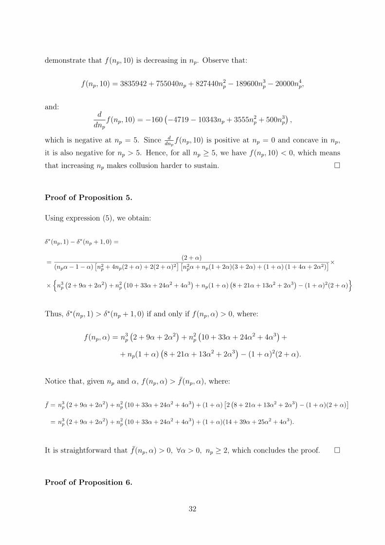
demonstrate that f(np, 10) is decreasing in np. Observe that:
f(np, 10) = 3835942 + 755040np + 827440n2p − 189600n3
p − 20000n4p,
and:d
dnpf(np, 10) = −160
(−4719− 10343np + 3555n2
p + 500n3p
),
which is negative at np = 5. Since ddnpf(np, 10) is positive at np = 0 and concave in np,
it is also negative for np > 5. Hence, for all np ≥ 5, we have f(np, 10) < 0, which means
that increasing np makes collusion harder to sustain.
Proof of Proposition 5.
Using expression (5), we obtain:
δ∗(np, 1)− δ∗(np + 1, 0) =
=(2 + α)
(npα− 1− α)[n2p + 4np(2 + α) + 2(2 + α)2
] [n2pα+ np(1 + 2α)(3 + 2α) + (1 + α) (1 + 4α+ 2α2)
]×
×n3p(2 + 9α+ 2α2
)+ n2p
(10 + 33α+ 24α2 + 4α3
)+ np(1 + α)
(8 + 21α+ 13α2 + 2α3
)− (1 + α)2(2 + α)
Thus, δ∗(np, 1) > δ∗(np + 1, 0) if and only if f(np, α) > 0, where:
f(np, α) = n3p
(2 + 9α + 2α2
)+ n2
p
(10 + 33α + 24α2 + 4α3
)+
+ np(1 + α)(8 + 21α + 13α2 + 2α3
)− (1 + α)2(2 + α).
Notice that, given np and α, f(np, α) > f(np, α), where:
f = n3p(2 + 9α+ 2α2
)+ n2p
(10 + 33α+ 24α2 + 4α3
)+ (1 + α)
[2(8 + 21α+ 13α2 + 2α3
)− (1 + α)(2 + α)
]
= n3p(2 + 9α+ 2α2
)+ n2p
(10 + 33α+ 24α2 + 4α3
)+ (1 + α)(14 + 39α+ 25α2 + 4α3).
It is straightforward that f(np, α) > 0, ∀α > 0, np ≥ 2, which concludes the proof.
Proof of Proposition 6.
32

(i) Consider a private oligopoly where the np + 1 private firms are colluding. From (17),
we obtain the individual collusive quantities:
qmp (np + 1, 0) =1− β
2(np + 1) + α.
Substituting this expression and qg = 0 in (1), we obtain the total surplus in a collusive
private oligopoly with np + 1 firms:
TSm(np + 1, 0) =(np + 1) [3(np + 1) + α] (1− β)2
2 [2(np + 1) + α]2. (28)
Consider now that the np + 1 private firms compete à la Cournot. From (22), we obtain
the individual non-cooperative output:
qcp(np + 1, 0) =1− β
np + 2 + α
Replacing this expression and qg = 0 in (1), we obtain the total surplus in a non-cooperative
private oligopoly with np + 1 firms:
TSc(np + 1, 0) =(np + 1)(np + 3 + α)(1− β)2
2(np + 2 + α)2. (29)
Substituting these expressions for total surplus in (8), we obtain:
Ω(np) = TSc(np + 1, 0)− TSm(np + 1, 0) =
=(1− β)2np(np + 1)
[n2p + np(5 + α) + 2(2 + α)
]
2(np + 2 + α)2 [2(np + 1) + α]2, (30)
which is positive.
(ii) Deriving expression (30) with respect to α, we obtain:
∂Ω
∂α= −(1− β)2np(np + 1)
[4n3
p + 7n2p(4 + α) + 3np(2 + α)(8 + α) + 6(2 + α)2
]
2(np + 2 + α)3 [2(np + 1) + α]3,
which is negative.
33

(iii) Let us now analyze the impact on an increase in np on Ω:
Ω(np + 1)− Ω(np) =(np + 1)(1− β)2
2(np + 2 + α)2(np + 3 + α)2 [2(np + 1) + α]2 [2(np + 2) + α]2×
×
8αn5p + 2n4
(16 + 48α+ 13α2
)+ n3
p
(240 + 504α+ 241α2 + 31α3
)+
+ n2p
(656 + 1312α+ 839α2 + 207α3 + 16α4
)+
+ np(2 + α)(384 + 616α+ 322α2 + 62α3 + 3α4
)+ 2(2 + α)4(10 + 3α)
.
As the expression above is positive, we conclude that Ω(np + 1) > Ω(np),∀np ≥ 2.
Proof of Proposition 7.
We analyze each of the following three scenarios in separate (see Figure 6):
A. Collusion is not sustainable neither before nor after privatization: δ < δ∗(np+1, 0).
B. Collusion is not sustainable before privatization but is sustainable afterward: δ∗(np+
1, 0) < δ < δ∗(np, 1).
C. Collusion is sustainable before and after privatization: δ > δ∗(np, 1).
Let ∆TSi denote the impact of privatization on total surplus in scenario i ∈ A,B,C,i.e., the difference between total surplus before and after privatization.
A. If collusion is not sustainable neither before privatization nor after privatization:
∆TSA = TSc(np + 1, 0)− TSc(np, 1). (31)
The expression for TSc(np + 1, 0) was already derived, in (29). Let us, then, derive the
expression for TSc(np, 1). Replacing ng = 1 in (22) and (23), we obtain the individual
outputs when there are np private firms and 1 public firm in the market:
qcp(np, 1) =α(1− β)
1 + α(np + 2) + α2and qcg(np, 1) =
(α + 1)(1− β)
1 + α(np + 2) + α2.
Replacing these expressions in (1), we obtain:
TSc(np, 1) =(1− β)2
[α2n2
p + αnp (2 + 4α + α2) + (1 + α)3]
2 [1 + (np + 2)α + α2]2. (32)
34

Replacing expressions (29) and (32) in (31), we obtain:
∆TSA =
[n2pα + npα− (1 + α)3
](1− β)2
2(np + 2 + α)2 [1 + (np + 2)α + α2]2.
Thus, privatization improves total surplus if and only if:
∆TSA > 0 ⇔ n2pα + npα− (1 + α)3 > 0 ⇔ np < n−p ∨ np > n+
p ,
where:
n−p =−α−
√α(1 + 2α) (4 + 5α + 2α2)
2αand n+
p =−α +
√α(1 + 2α) (4 + 5α + 2α2)
2α.
It follows immediately that n−p < 0. We now need to check whether n+p is lower or greater
than 2:
n+p ≥ 2 ⇔ −5α +
√α(1 + 2α) (4 + 5α + 2α2) > 0
⇔ α(1 + 2α)(4 + 5α + 2α2
)> 25α2 ⇔ 4α
(1− 3α + 3α2 + α3
)> 0
⇔ 1− 3α + 3α2 + α3 > 0
Let f(α) = 1− 3α + 3α2 + α3. Hence:
f ′(α) = 0 ⇔ 3(−1 + 2α + α2
)= 0 ⇔ α = −1±
√2
Thus, if restricted to α > 0, f as a global minimum at α = −1 +√
2. As f(−1 +√
2) =
2(3− 2
√2)> 0, we conclude that: f(α) > 0,∀α ≥ 0. This implies that n+
p > 2,∀α ≥ 0.
Manipulating the expression for n+p , we find that privatization increases total surplus iff:
np >1
2
[√(1 + 2α) (4 + 5α + 2α2)
α− 1
].
B. If collusion is not sustainable before privatization but is sustainable after:
∆TSB = TSm(np + 1, 0)− TSc(np, 1),
35

where expressions for TSm(np + 1, 0) and TSc(np, 1) are given in (28) and (32). Thus:
∆TSB = − (1− β)2
2 [(2(np + 1) + α]2 [1 + (np + 2)α + α2]2×
×n4pα
2 + n3pα(2 + 6α + α2
)+ n2
p
(1 + 4α + 9α2 + 3α3
)+
+ np(2 + α)(1 + 2α + 2α2
)+ (1 + α)3
,
which implies that privatization is detrimental to total surplus, regardless of np and α.
C. If collusion is sustainable either before and after privatization:
∆TSC = TSm(np + 1, 0)− TSm(np, 1),
where expressions for TSm(np + 1, 0) is given in (28). Replacing ng = 1 in (17) and (18),
we obtain the individual output levels before privatization:
qmp (np, 1) =α(1− β)
np + α(2np + 1) + α2and qmg (np, 1) =
(np + α)(1− β)
np + α(2np + 1) + α2
Replacing these expressions in (1), we obtain:
TSm(np, 1) =(1− β)2
[n2p (1 + 3α + 3α2) + npα (2 + 4α + α2) + α2(1 + α)
]
2 [np + α(2np + 1) + α2]2.
Hence:
∆TSC = − (1− β)2[n4p + n3p
(2 + 5α+ 6α2
)+ n2p
(1 + 7α+ 12α2 + 3α3
)+ npα
(2 + 6α+ 3α2
)+ α2(1 + α)
]
2(2 + 2np + α)2 [np + α(2np + 1) + α2]2 ,
which is straightforwardly negative.
Corollary 2. If there are initially two private firms and one public firm in the market,
total surplus decreases with privatization.
Proof. From Proposition 7, we know that privatization may only increase total surplus if
36

condition (9) is satisfied. Replace np = 2 in that condition and notice that:
1
2
[√(1 + 2α) (4 + 5α + 2α2)
α− 1
]< 2 ⇔ (1 + 2α)
(4 + 5α + 2α2
)< 25α ⇔
⇔ 4(1− 3α + 3α2 + α3
)< 0.
Let f(α) = 1− 3α + 3α2 + α3. Therefore, f ′(α) = 0 ⇔ α = −1−√
2 ∨ α = −1 +√
2.
Thus, we conclude that f has a local minimum at α = −1 +√
2. As f(0) > 0 and
f(−1 +√
2) > 0, we conclude that f(α) > 0, ∀α ≥ 0.
Proof of Proposition 8.
The semi-public firm produces the quantity, Qs, that maximizes (10), i.e., that solves
θ ∂TS∂Qg
+ (1 − θ)∂πg∂qg
= 0. Thus, given the output produced by the private sector, Qp, the
best-response of the semi-public firm is:
Qs (Qp) =1
α− θ + 2(1− β −Qp). (33)
We now derive the individual profits of private firms in each scenario.
1. Collusive profits
Combining the best-reply function of the two sectors, given by (33) and (16), we obtain:
Qmp =
(1− β)(1− θ + α)npnp(3− 2θ + 2α) + α(2− θ + α)
and Qmg =
(1− β)(np + α)
np(3− 2θ + 2α) + α(2− θ + α).
(34)
Replacing these quantities in (20), we obtain the collusive profit of a private firm:
πmp =(1− β)2(1− θ + α)2(2np + α)
2[np(3− 2θ + 2α) + α(2− θ + α)]2. (35)
2. Deviation profits
Suppose now that firm i ∈ 1, 2, ..., np deviates and produces the quantity that maximizes
its individual profit. More precisely, the firm chooses qdp that maximizes (25) with qmp =Qmpnp
,
37

and Qmp and Qm
g given by (34). Solving the corresponding FOC and replacing the obtained
quantity in the profit function of firm i, we obtain its deviation profit:
πdp =(1− β)2(1− θ + α)2(np + 1 + α)2
2(2 + α) [np(3− 2θ + 2α) + α(2− θ + α)]2.
3. Punishment profits
Combining the best-reply function of the public firm, (33), with the best-reply function
of the private sector when behaving non-cooperatively, (21), we obtain the (aggregate)
output levels of the private and the public sectors, Qcp and Qc
g. Replacing these quantities
in (20), we obtain the profit of a private firm in a period along the punishment path:
πcp =(2 + α)(1− β)2(1− θ + α)2
2 [np(1− θ + α) + (1 + α)(2− θ + α)]2.
4. Profit comparison
Comparing profits along the collusive and the punishment paths:
πcp < πm
p ⇔(np − 1)(1− β)2(1− θ + α)2
2 [np(1− θ + α) + (1 + α)(2− θ + α)]2
[np(3− 2θ + 2α) + α(2− θ + α)]2×
×− 2n2p(1 + α− θ)2 + np(2− θ + α)
(4− α2 − 2θ + α(2 + θ)
)+ α(2− θ + α)2
> 0.
Note that the fraction in the LHS of the last inequality is always positive. The roots of
the second-order polynom inside the curly brackets are:
n±p =2 + α− θ
4(1 + α− θ)2
[4− 2θ + α(2− α + θ)±
√[4− 2θ + α(2− α + θ)]2 + 8α(1 + α− θ)2
].
It is straightforward that n−p < 0. Hence, πcp < πmp if and only if np > n+p .
To obtain the expression for the critical discount factor, replace expressions for individual
profits in the ICC (4), and simplify the expression.
Proof of Corollary 1.
38

The derivative of the critical discount factor, given in (11), with respect to θ is:
∂δ?
∂θ=
2(2 + α)2np(np − 1) [np(3− 2θ + 2α) + α(2− θ + α)] [np(1− θ + α) + (1 + α)(2− θ + α)]
D2,
where:
D = n3p(1− θ + α)2 + n2
p(1− θ + α)(7 + 11α + 4α2 − 5θ − 4αθ
)+
+ np(2− θ + α)[2α3 + 2α2(1− θ)− 7α− 8 + 5θ
]−(1 + 4α + 2α2
)(2− θ + α)2.
It follows that ∂δ?
∂θ> 0.
Impact of an additional private firm on collusion sustainability (Figure 9).
Using expression (11) for the critical discount factor, we have:
δ?(np + 1, 1)− δ?(np, 1) =(2 + α)×ND1 ×D2
,
with:
N = 2n4p(1− θ + α)4 + 2n3p(1− θ + α)2[α3 + 2α2(1− θ)− α
(4 + 2θ − θ2
)− 2(3− 2θ)
]−
− n2p(1− θ + α)[5α4 + α3(41− 13θ) + α2(2− θ)(56− 11θ) + α
(122− 136θ + 41θ2 − 3θ3
)+
+ 2(23− 35θ + 16θ2 − 2θ3
) ]−
− np(1− θ + α)(2− θ + α)[5α3 + α2(21− 4θ) + 2
(4− θ − θ2
)+ α
(24− 7θ − θ2
)]−
− 2(1 + α)2(2− θ + α)2[α2 + α(4− θ) + 3− 2θ
]
D1 = [(np − 1)(1− θ + α)− 1][n2p(1− θ + α) + np(3 + 2α)(3 + 2α− 2θ) +
(1 + 4α+ 2α2
)(2 + α− θ)
]
D2 = [np(1− θ + α)− 1]n2p(1− θ + α) + np
[4α2 + 2α(7− 2θ) + 11− 8θ
]+
+ 2(2 + α)[α2 + α(4− θ) + 3− 2θ
] .
As D1 and D2 are both positive, we conclude that:
δ?(np + 1, 1) > δ?(np, 1) ⇔ N > 0.
Proof of Proposition 9.
39

As in the proof of Proposition 7, we distinguish 3 scenarios, depending on the sustainability
of collusion before and after privatization and denote by ∆TS?i the impact of privatization
on total surplus, in scenario i ∈ A,B,C, when the semi-public firm maximizes (10).
A. If collusion is not sustainable neither before privatization nor after privatization:
∆TS?A = TSc?(np + 1, 0)− TSc?(np, 1)
=(1− β)2θ
2(np + 2 + α)2(np(1− θ + α) + (1 + α)(2− θ + α))2×
×n2pαθ − np
[2(1 + α2
)(1− θ) + α(4− 5θ)
]− (1 + α)2 [4− 3θ + α(2− θ)]
.
Thus:
∆TS?A > 0 ⇔ n2pαθ − np
[2(1 + α2
)(1− θ) + α(4− 5θ)
]− (1 + α)2 [4− 3θ + α(2− θ)] > 0.
Solving the previous condition (under the restriction that np > 0), we obtain that TSc?(np+
1, 0) > TSc?(np, 1) if and only if:
np >1
2αθ
2(1 + α2
)(1− θ) + α(4− 5θ) +
√[2 (1 + α2) (1− θ) + α(4− 5θ)]2 + 4αθ(1 + α)2[4− 3θ + α(2− θ)]
.
B. If collusion is not sustainable before privatization but it is sustainable after:
∆TS?B = TSm?(np + 1, 0)− TSc?(np, 1)
= −1
2
[1− β
[2(np + 1) + α] [np(1− θ + α) + (1 + α)(2− θ + α)]
]2
× A
with:
f = n4p(1− θ + α)2 + n3
p(1− θ + α)[α2 + α(7− θ) + 2(3− 2θ)
]+
+ n2p
[3α3 + α2(15− 6θ) + α
(21− 16θ − θ2
)+ 9− 10θ + 2θ2
]+
+ np
2α3 + 2α2[2(2− θ2
)+ θ]
+ α[10(1− θ2
)+ θ(4 + θ)
]+ 2
[2(1− θ2
)+ θ]
+
+ (1 + α)2θ [4(1− θ) + α(2− θ) + θ] .
As f > 0, we conclude that TSm?(np + 1, 0) < TSc?(np, 1).
40

C. If collusion is sustainable either before and after privatization:
∆TS?C = TSm?(np + 1, 0)− TSm?(np, 1)
= − 1
2
[1− β
[2(np + 1) + α] [np(3− 2θ + 2α) + α(2− θ + α)]
]2
× g
with:
g = n4p(5− 4θ) + n3
p
[6α2 + α(23− 18θ) + 2(5− 4θ)
]+
+ n2p
[3α3 + 4α2(5− 2θ) + α
(23− 8θ − 8θ2
)+ 5− 4θ
]+
+ npα[3α2 + 6α(1 + θ(1− θ)) + 2θ(5− 4θ)
]+ α2θ [(4− 3θ + α(2− θ)] .
As g > 0, we conclude that TSm?(np + 1, 0) < TSm?(np, 1).
Proof of Proposition 10.
Consider a symmetric punishment according to which all private firms produce the same
quantity, qp, with qp > qcp > qmp , in the punishment period. Using the best-reply function
of the public firm (2), the profit of a private firm if the punishment is executed is:
πpp(qp) =
(1− β − npqp −
1− β − npqpα + 1
)qp − α(qp)2
2. (36)
A private firm unilaterally deviating from the punishment would produce:
qdpp (qp) =α(1− β) + (1 + α− αnp)qp
(α + 2)(α + 1), (37)
and its profit would be:
πdpp (qp) =α(1− β) + [1− α(np − 1)]qp2
2(α + 2)(α + 1)2. (38)
A stronger punishment (greater qp) relaxes the ICC (12) for collusion to be sustainable,
but tightens the ICC (13) for the punishment to be credible. Setting α = 3 (which implies
that collusion is profitable), this can easily be verified.
Hence, the lowest possible critical discount factor is attained when qp is such that the two
41

ICCs are satisfied in equality. For α = 3:
πdp − πmpπmp − πpp(qp)
=πdpp (qp)− πpp(qp)πmp − πpp(qp)
⇒ qp =3(1− β) (11np + 8)
21n2p + 148np + 192
.
Replacing this expression for qp, we obtain the critical discount factor:
δop =πdp − πmp
πmp − πpp(qp)=πdpp (qp)− πpp(qp)πmp − πpp(qp)
=(np − 1) (3np + 16)2
20 (3np − 4) (7np + 12).
The expressions used above are valid if np ≤ 14. If np ≥ 15, the expression used for the
output of the public firm would give a negative value.
References
Abreu, D. (1986). Extremal equilibria of oligopolistic supergames. Journal of Economic
Theory, 39(1):191–225.
Anderson, S. P., De Palma, A., and Thisse, J.-F. (1997). Privatization and efficiency in a
differentiated industry. European Economic Review, 41(9):1635–1654.
Barca, F. and Becht, M. (2001). The control of corporate Europe. Oxford University Press.
Barros, F. (1995). Incentive schemes as strategic variables: an application to a mixed
duopoly. International Journal of Industrial Organization, 13(3):373–386.
Barros, P. P. and Martinez-Giralt, X. (2002). Public and private provision of health care.
Journal of Economics & Management Strategy, 11(1):109–133.
Beato, P. and Mas-Colell, A. (1984). Marginal cost pricing rule as a regulation mecha-
nism in mixed markets. In Marchand, M., Pestieau, P., and Tulkens, H., editors, The
Performance of Public Enterprise. North-Holland.
Bös, D. (1987). Privatization of public enterprises. European Economic Review, 31(1-
2):352–360.
Brandão, A. and Castro, S. (2007). State-owned enterprises as indirect instruments of
entry regulation. Journal of Economics, 92(3):263–274.
42

Colombo, S. (2016). Mixed oligopolies and collusion. Journal of Economics, 118(2):167–
184.
Cremer, H., Marchand, M., and Thisse, J.-F. (1989). The public firm as an instrument
for regulating an oligopolistic market. Oxford Economic Papers, 41(2):283–301.
De Fraja, G. and Delbono, F. (1989). Alternative strategies of a public enterprise in
oligopoly. Oxford Economic Papers, 41(2):302–311.
De Fraja, G. and Delbono, F. (1990). Game theoretic models of mixed oligopoly. Journal
of Economic Surveys, 4(1):1–17.
Delbono, F. and Lambertini, L. (2016). Nationalization as credible threat against collusion.
Journal of Industry, Competition and Trade, 16(1):127–136.
Dijkgraaf, E. and Gradus, R. (2007). Collusion in the Dutch waste collection market.
Local Government Studies, 33(4):573–588.
Fershtman, C. and Judd, K. L. (1987). Equilibrium incentives in oligopoly. American
Economic Review, 77(5):927–940.
Fjell, K. and Heywood, J. S. (2004). Mixed oligopoly, subsidization and the order of firm’s
moves: the relevance of privatization. Economics Letters, 83(3):411–416.
Friedman, J. W. (1971). A non-cooperative equilibrium for supergames. Review of Eco-
nomic Studies, 38(1):1–12.
George, K. and La Manna, M. M. (1996). Mixed duopoly, inefficiency, and public owner-
ship. Review of Industrial Organization, 11(6):853–860.
Hamilton, J. H. and Slutsky, S. M. (1990). Endogenous timing in duopoly games: Stack-
elberg or Cournot equilibria. Games and Economic Behavior, 2(1):29–46.
Haraguchi, J. and Matsumura, T. (2016). Cournot-Bertrand comparison in a mixed
oligopoly. Journal of Economics, 117(2):117–136.
Harris, R. G. and Wiens, E. G. (1980). Government enterprise: an instrument for the
internal regulation of industry. Canadian Journal of Economics, 13(1):125–132.
43

Ivaldi, M., Jullien, B., Rey, P., Seabright, P., and Tirole, J. (2007). The economics of tacit
collusion: implications for merger control. In Ghosal, V. and Stennek, J., editors, The
Political Economy of Antitrust. Elsevier.
Lin, M. H. and Matsumura, T. (2012). Presence of foreign investors in privatized firms
and privatization policy. Journal of Economics, 107(1):71–80.
Magnus, E. and Midttun, A. (2000). The Norwegian model: competitive public economy.
In Electricity Market Reform in Norway. Palgrave Macmillan UK, London.
Matsumura, T. (1998). Partial privatization in mixed duopoly. Journal of Public Eco-
nomics, 70(3):473–483.
Matsumura, T. (2003). Stackelberg mixed duopoly with a foreign competitor. Bulletin of
Economic Research, 55(3):275–287.
Matsumura, T. and Kanda, O. (2005). Mixed oligopoly at free entry markets. Journal of
Economics, 84(1):27–48.
Matsumura, T. and Okamura, M. (2015). Competition and privatization policies revisited:
the payoff interdependence approach. Journal of Economics, 116(2):137–150.
Matsumura, T. and Shimizu, D. (2010). Privatization waves. The Manchester School,
78(6):609–625.
Matsushima, N. and Matsumura, T. (2006). Mixed oligopoly, foreign firms, and location
choice. Regional Science and Urban Economics, 36(6):753–772.
Megginson, W. L. and Netter, J. M. (2001). From state to market: A survey of empirical
studies on privatization. Journal of Economic Literature, 39(2):321–389.
Merrill, W. C. and Schneider, N. (1966). Government firms in oligopoly industries: a
short-run analysis. Quarterly Journal of Economics, 80(3):400–412.
Motta, M. (2004). Competition policy: theory and practice. Cambridge University Press.
Naya, J. M. (2015). Endogenous timing in a mixed duopoly model. Journal of Economics,
116(2):165–174.
Nett, L. (1993). Mixed oligopoly with homogeneous goods. Annals of Public and Cooper-
ative Economics, 64(3):367–393.
44

OECD (2005). Corporate governance of state-owned enterprises: a survey of OECD coun-
tries. Technical report, Organisation for Economic Co-operation and Development,
Paris.
Pal, D. (1998). Endogenous timing in a mixed oligopoly. Economics Letters, 61(2):181–185.
Perry, M. and Porter, R. (1985). Oligopoly and the incentive for horizontal merger. Amer-
ican Economic Review, 75:219–227.
Salant, S. W., Switzer, S., and Reynolds, R. J. (1983). Losses from horizontal merger:
the effects of an exogenous change in industry structure on Cournot-Nash equilibrium.
Quarterly Journal of Economics, 98(2):185–199.
Sertel, M. R. (1988). Regulation by participation. Journal of Economics, 48(2):111–134.
Singh, N. and Vives, X. (1984). Price and quantity competition in a differentiated duopoly.
RAND Journal of Economics, 15(4):546–554.
Sklivas, S. D. (1987). The strategic choice of managerial incentives. RAND Journal of
Economics, 18(3):452–458.
Starr, P. (1988). The meaning of privatization. Yale Law & Policy Review, 6(1):6–41.
Vickers, J. and Yarrow, G. (1991). Economic perspectives on privatization. Journal of
Economic Perspectives, 5(2):111–132.
45

Editorial Board ([email protected])Download available at: http://wps.fep.up.pt/wplist.php
also in http://ideas.repec.org/PaperSeries.html
47


49