Collateralized Debt Obligation (CDO) modelling and its model comparisons

Yang Yi

1544020

BMI‐paper Vrije Universiteit Faculty of Sciences De Boelelaan 1081a 1081 HV Amsterdam

Supervisor: Prof. dr. Andre Lucas

1

Abstract Since CDO pricing issue attracts more attention these years, many researchers are devoted themselves to the pricing model studies. In practice, standard Gaussian copula model becomes the market standard in the financial filed. However, due to its weakness of mispricing, many extension models are researches, such as student t copula, Clayton copula, factor loading Gaussian copula, implied copula approach etc. They all show improvements to the Gaussian copula in terms of fitting to the market quotes, yet with different performances. This paper mainly addresses the pricing models for CDO tranche available so far, and presents its model comparisons with merits and disadvantages.

2

Contents 1. Introduction .................................................................................................................. 5

2. Credit derivatives........................................................................................................ 6

2.1 Brief overview ........................................................................................................ 6 2.2 Instruments ............................................................................................................. 6 2.2.1 Credit default swap ............................................................................................ 7 2.2.2 Asset swaps........................................................................................................ 8 2.2.3 Total return swaps............................................................................................. 9 2.2.4 Credit linked notes ........................................................................................... 10 2.2.5 Collateralized Debt Obligation ........................................................................ 11

3. Synthetic CDO tranche and its valuation ............................................................... 14

3.1 Basic knowledge about CDO tranches.............................................................. 14 3.2 Valuation methodology of synthetic CDO tranche......................................... 16 3.2.1 Loss distribution introduction......................................................................... 16 3.2.2 Pricing synthetic CDO tranche using General semi‐analytic approach......... 18

4. Copula Function and default correlation model (factor copula model) ............ 20

4.1 Definition and Basic Properties of Copula Function ...................................... 20 4.2 Default correlation model (factor copula model) ............................................ 21

5. One factor Gaussian copula model ......................................................................... 24

5.1 One factor Gaussian copula model set up........................................................ 24 5.2 Loss distribution................................................................................................... 25 5.2.1 Conditional loss probability ............................................................................. 25 5.2.2 Unconditional loss distributions ..................................................................... 26

5.3 The large portfolio approximation for the one factor model......................... 27 5.4 Evaluation of the Gaussian copula approach .................................................. 28 5.4.1 Correlation structure ....................................................................................... 28 5.4.2 Correlation smile............................................................................................ 29

6. Extensions to the Gaussian model and its comparisons ...................................... 31

6.1 Student t copula model ....................................................................................... 31 6.2 Double t copula model ........................................................................................ 32 6.3 Clayton copula model ......................................................................................... 33 6.4 Normal inverse Gaussian model ....................................................................... 33 6.4.1 Definition and properties of the NIG distribution........................................... 34 6.4.2 Normal inverse model set up ........................................................................... 35

3

6.5 Stochastic correlation Gaussian models ........................................................... 36 6.6 Random factor loading (RFL) model ................................................................ 37 6.6.1 Model set up..................................................................................................... 37 6.6.2 Gaussian copula with RFL .............................................................................. 38

6.7 Perfect copula ....................................................................................................... 42 6.7.1 Implied hazard rate paths................................................................................. 42 6.7.2 Implied copula approach .................................................................................. 43

7. Comparison of various pricing models .................................................................. 45

8. Conclusion .................................................................................................................. 48

References........................................................................................................................ 50

4

1. Introduction With the market of credit derivatives grows larger, collateralized debt obligations (CDOs) as one of their most popular instruments also gain more interests both from the market side and the academic side. Though it appears a dramatic increase in the traded CDO contracts, unfortunately, achieving a precise CDO tranche valuation is still a difficult and an open issue today. This paper explores the vast area of the credit derivatives and the literatures on the pricing models of collateralized debt obligations (CDOs). I aim at gaining insight in the financial as well as mathematical foundation of the credit derivatives and CDO pricing models. In order to obtain the fair premium of the CDO tranche, the market standard pricing model‐‐‐one factor Gaussian copula model, and its various extension models (e.g. student t, double t, factor loading, normal inverse copula, perfect copula etc) are presented. Besides considering the model selection, I also discuss about the comparisons of model performances, its advantages and weakness. The rest of the paper is structured as follows: chapter 2 gives to a general overview of credit derivatives. In particular, some of the most popular credit derivative instruments are addressed. Chapter 3 focuses on the basic knowledge about the synthetic CDO tranche and its valuation methodology using general semi‐analytic approach. Particularly, I discuss a few concepts and their relationships, such as loss distribution, large portfolio approximation and default correlation. They are crucial for calculating the fair premium of CDO tranche. In chapter 4, I present the copula function and default correlation models (factor copula model), which constructs a general framework for various pricing models discussed in the next few chapters. Then, chapter 5 elaborates on the market standard pricing model‐‐‐one factor Gaussian copula model, including its conditional/unconditional loss distribution functions, large portfolio approximations and evaluation issues. It is argued that despite Gaussian copula model is widespread deployed in the market nowadays; they do show many shortcomings. Some of those even lead to serious consequence of huge mispricing discrepancy. Subsequently, the possible reasons for mispricing are also presented, such as the well‐known correlation smile. Considering the insufficiencies of the market standard model, various extension copula models are presented in chapter 6, which aim at reproducing the correlation skew and fit the market quote better. In chapter 7, model comparisons based on abilities of the different models to reproduce market quotes are discussed. Finally, conclusions are drawn in chapter 8. It shows that most extension models have improvements

5

compared to Gaussian copula models, particularly for the following three copula models display best fit the market quote. They are ‘factor loading Gaussian copula model’, ‘normal inverse Gaussian copula model’, and the implied copula approach (or perfect copula).

2. Credit derivatives

2.1 Brief overview

Credit derivatives were introduced to the market at the beginning of the 1990’s. Despite their short history, their uses have grown rapidly. They are now used not only by banks, but also by various funds, insurance companies, and even corporations.

By definition, ‘credit derivatives are a group of financial instruments that have as their common main purpose the managing of credit exposures, and thus credit or default risk’ (Jonathan Batten, Warren Hogan, 2002).

As a very useful tool, credit derivative enable the investors to transfer and diversify credit risk. Specifically, for the lenders, such as a commercial bank, who want to reduce their exposure to a particular borrower, but are unwilling to sell their ownerships of underlying assets to the borrower, credit derivatives contracts may be a wise choice. Since it successfully realizes the function of transferring the credit risk without actually transferring the ownership.

Credit derivatives come in many shapes and sizes, and there are several ways of grouping them. Here I introduce the primary category: single‐name versus multi‐name credit derivatives. Single‐name credit derivatives are those involving protection against the default by a single reference entity, such as a credit default swap (CDS). Multi‐name credit derivatives are the contracts that are contingent on default events by a pool of reference entities. A simple example is the portfolio default swaps, and the collateralized debt obligations (CDOs).

2.2 Instruments In the vast area of the credit derivatives world, there are many types of products. This chapter is devoted to the overview of several important credit derivative instruments based on the background knowledge in Bomfim, A.N. 2005.

6

2.2.1 Credit default swap

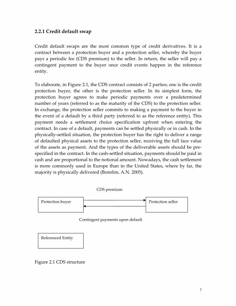
Credit default swaps are the most common type of credit derivatives. It is a contract between a protection buyer and a protection seller, whereby the buyer pays a periodic fee (CDS premium) to the seller. In return, the seller will pay a contingent payment to the buyer once credit events happen in the reference entity.

To elaborate, in Figure 2.1, the CDS contract consists of 2 parties; one is the credit protection buyer, the other is the protection seller. In its simplest form, the protection buyer agrees to make periodic payments over a predetermined number of years (referred to as the maturity of the CDS) to the protection seller. In exchange, the protection seller commits to making a payment to the buyer in the event of a default by a third party (referred to as the reference entity). This payment needs a settlement choice specification upfront when entering the contract. In case of a default, payments can be settled physically or in cash. In the physically‐settled situation, the protection buyer has the right to deliver a range of defaulted physical assets to the protection seller, receiving the full face value of the assets as payment. And the types of the deliverable assets should be pre‐specified in the contract. In the cash‐settled situation, payments should be paid in cash and are proportional to the notional amount. Nowadays, the cash settlement is more commonly used in Europe than in the United States, where by far, the majority is physically delivered (Bomfim, A.N. 2005).

Figure 2.1 CDS structure

Protection buyer

CDS premium

Protection seller

Contingent payments upon default

Referenced Entity

7

2.2.2 Asset swaps The asset swap is a common form of a derivative contract1, in which, an investor (asset swap buyer) can buy a fixed rate liability (usually a coupon bond) issued by a reference entity and simultaneously enter an interest rate swap, where the fixed rate and maturity date exactly match those of the fixed‐rate liability. At the maturity date, the investor of the asset swap effectively transfers the interest rate (market) risk of the fixed rate liability to its asset swap counterparty (or dealer or asset swap seller), retaining only the credit risk component. As such, we obtain one important characteristic of asset swaps: allowing investors to take pure credit positions. In other words, asset swaps can be used for investors who are willing to take exposure to credit risk without worrying about the interest risks. To elaborate, we can decompose the process into the following two parts:

Purchasing the fixed rate bond at par value

The investor (asset swap buyer) agrees to buy from the dealer (asset swap seller) a fixed rate bond issued by the reference entity, paying for the par value regardless of the market value.

Entering the interest rate swap

Figure 2.2 asset swap The investor (asset swap buyer) pays for the dealer’s (asset swap seller) periodic fixed rate payments, which are equal to the amount of the coupon paid by

1 so far, there is still some disagreement on whether the asset swap is a credit derivative

Asset swap buyer Asset swap seller

Coupon payment

LIBOR + asset swap spread

Fixed rate bond

Coupon

Asset swap buyer

Par value

Asset swap seller

Fixed rate bond

8

reference bond (fixed rate bond). In return, the asset swap seller will make variable interest rate payments to the investor, which is equal to the amount: Libor plus asset swap spread2. In such a way, investor successfully transfers the interest risk retaining merely the credit risk.

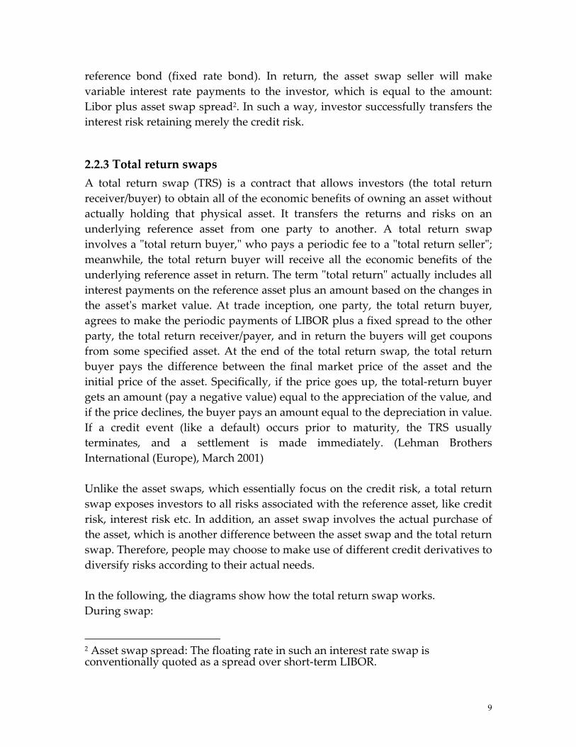
2.2.3 Total return swaps A total return swap (TRS) is a contract that allows investors (the total return receiver/buyer) to obtain all of the economic benefits of owning an asset without actually holding that physical asset. It transfers the returns and risks on an underlying reference asset from one party to another. A total return swap involves a ʺtotal return buyer,ʺ who pays a periodic fee to a ʺtotal return sellerʺ; meanwhile, the total return buyer will receive all the economic benefits of the underlying reference asset in return. The term ʺtotal returnʺ actually includes all interest payments on the reference asset plus an amount based on the changes in the assetʹs market value. At trade inception, one party, the total return buyer, agrees to make the periodic payments of LIBOR plus a fixed spread to the other party, the total return receiver/payer, and in return the buyers will get coupons from some specified asset. At the end of the total return swap, the total return buyer pays the difference between the final market price of the asset and the initial price of the asset. Specifically, if the price goes up, the total‐return buyer gets an amount (pay a negative value) equal to the appreciation of the value, and if the price declines, the buyer pays an amount equal to the depreciation in value. If a credit event (like a default) occurs prior to maturity, the TRS usually terminates, and a settlement is made immediately. (Lehman Brothers International (Europe), March 2001) Unlike the asset swaps, which essentially focus on the credit risk, a total return swap exposes investors to all risks associated with the reference asset, like credit risk, interest risk etc. In addition, an asset swap involves the actual purchase of the asset, which is another difference between the asset swap and the total return swap. Therefore, people may choose to make use of different credit derivatives to diversify risks according to their actual needs. In the following, the diagrams show how the total return swap works. During swap:

2 Asset swap spread: The floating rate in such an interest rate swap is conventionally quoted as a spread over short‐term LIBOR.

9

Coupon from references asset

Total return seller/payer

Total return buyer/receiver

Libor + fixed spread

At maturity:

Figure 2.3 Total return swap

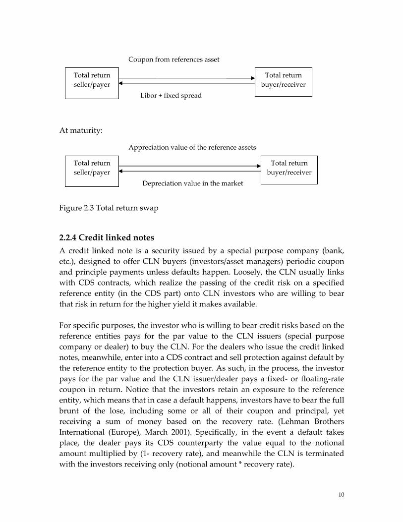
2.2.4 Credit linked notes A credit linked note is a security issued by a special purpose company (bank, etc.), designed to offer CLN buyers (investors/asset managers) periodic coupon and principle payments unless defaults happen. Loosely, the CLN usually links with CDS contracts, which realize the passing of the credit risk on a specified reference entity (in the CDS part) onto CLN investors who are willing to bear that risk in return for the higher yield it makes available. For specific purposes, the investor who is willing to bear credit risks based on the reference entities pays for the par value to the CLN issuers (special purpose company or dealer) to buy the CLN. For the dealers who issue the credit linked notes, meanwhile, enter into a CDS contract and sell protection against default by the reference entity to the protection buyer. As such, in the process, the investor pays for the par value and the CLN issuer/dealer pays a fixed‐ or floating‐rate coupon in return. Notice that the investors retain an exposure to the reference entity, which means that in case a default happens, investors have to bear the full brunt of the lose, including some or all of their coupon and principal, yet receiving a sum of money based on the recovery rate. (Lehman Brothers International (Europe), March 2001). Specifically, in the event a default takes place, the dealer pays its CDS counterparty the value equal to the notional amount multiplied by (1‐ recovery rate), and meanwhile the CLN is terminated with the investors receiving only (notional amount * recovery rate).

Total return seller/payer

Appreciation value of the reference assets

Total return buyer/receiver

Depreciation value in the market

10

Figure 2.4 Credit linked notes

2.2.5 Collateralized Debt Obligation A collateralized debt obligation (CDO) is defined as a structured financial product backed by portfolios of assets. Those assets are called collateral, which usually includes a combination of debt instruments or loans, such as bonds, loans, asset‐backed securities, etc. When the collaterals are loans, the CDO is called a collateralized loan obligation (CLO); if they are bonds, it turns to be a CBO (collateralized bond obligation). A CDO has a sponsoring organization, which sets up a specially created company, namely a special purpose vehicle (SPV) in order to hold the collateral and issue securities to investors. The sponsoring organization may contain sponsoring banks and other financial institutions. There are multiple tranches of securities issued by the CDO (SPV), offering investors various maturity and credit risk characteristics based on the collaterals assets. And according to the level of credit risk, tranches are then categorized as senior, mezzanine, and subordinated/equity (from the lowest to the highest degree of credit risk). If there are defaults or underperforms of the CDOʹs collateral, the investor who buys the equity tranche has to first bear the loss, and then the mezzanine and the senior tranche. In other words, the payments to senior tranches take precedence over those of mezzanine tranches, and the payments to mezzanine tranches take precedence over those to subordinated/equity tranches. Essentially, by selling these securitized collateral assets in the form of tranched securities, the issuer (SPV) transfers the complete credit risk of the collateral pool to the investors. To elaborate, a simple CDO example with a figure is made in the following.

Par value

Protection buyer

CDS Premium

Dealer/bank/ CLN issuer

Investor /asset managers

Reference entity

Protection

Coupon + principle

Credit linked notes

11

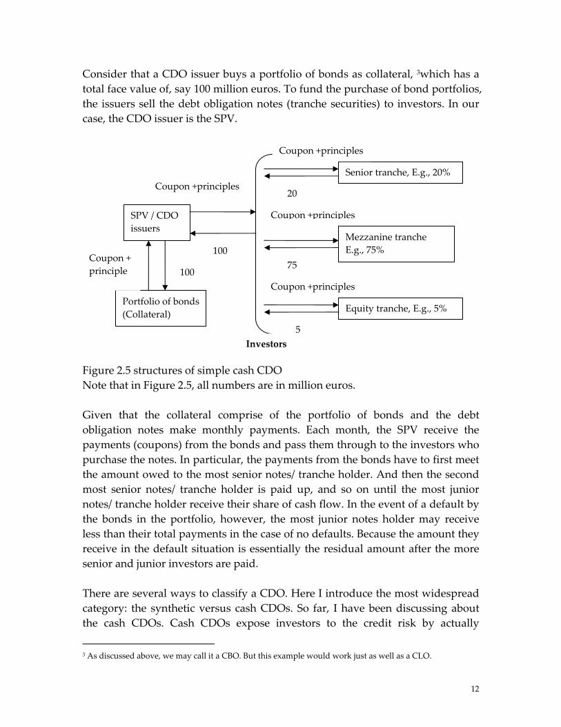
Consider that a CDO issuer buys a portfolio of bonds as collateral, 3which has a total face value of, say 100 million euros. To fund the purchase of bond portfolios, the issuers sell the debt obligation notes (tranche securities) to investors. In our case, the CDO issuer is the SPV.

Figure 2.5 structures of simple cash CDNote that in Figure 2.5, all numbers are Given that the collateral comprise oobligation notes make monthly paympayments (coupons) from the bonds anpurchase the notes. In particular, the pathe amount owed to the most senior nomost senior notes/ tranche holder is pnotes/ tranche holder receive their sharthe bonds in the portfolio, however, tless than their total payments in the casreceive in the default situation is essensenior and junior investors are paid. There are several ways to classify a CDcategory: the synthetic versus cash CDthe cash CDOs. Cash CDOs expose

3 As discussed above, we may call it a CBO. But this

Portfolio of bonds (Collateral)

SPV / CDO issuers

Coupon + principle 100

Invest

Coupon +principles

C

100

C

Coupon +principles

O in million euros.

f the portfolio of bonds and the debt ents. Each month, the SPV receive the d pass them through to the investors who yments from the bonds have to first meet tes/ tranche holder. And then the second aid up, and so on until the most junior e of cash flow. In the event of a default by he most junior notes holder may receive e of no defaults. Because the amount they tially the residual amount after the more

O. Here I introduce the most widespread Os. So far, I have been discussing about investors to the credit risk by actually

example would work just as well as a CLO.

Senior tranche, E.g., 20%

ors

Mezzanine tranche E.g., 75%

Equity tranche, E.g., 5%

20

oupon +principles

75

oupon +principles

5

12

holding the collateral that is subject to defaults. By comparison, the synthetic CDO holds the high quality or cash collateral that has little or no default risk. It exposes investors to credit risk by adding credit default swaps (CDSs) to the collateral. So the synthetic CDO is actually backed by serials of single name CDS. A simple example with diagram is made as following. Consider a commercial bank (as sponsoring bank in the diagram) with a bond portfolio of 100 million euros, which can be seen as the reference assets.

FNC TisthbCpstexpS

Sponsoring bank

A serial of CDS C+P

CDO cash flow

Senior tranche,

100

E.g., 20%

Mezzanine tranche E.g., 75%

19.6CDS premium

C+PSPV

98

73.5C+P Protection

+

C

igure 2.6 Synthetic CDO structure ote that in Figure 2.6, all numbers are in million euros. +P : means coupon + principles

he bank wants to transfer its credit risks associated with the bond portfolio, but not willing to sell them to the SPV. In other words, the bank tends to sell only e credit risk related to the bond portfolio (reference assets) and still keep the onds in its balance sheet. The transfer of the risk is carried out by a serials of DS, where the SPV is the counterparty and where the sponsoring bank buys a rotection of any loss in excess of, say, 2% of the portfolio. As in the cash CDO ructure, the SPV then issues the notes to various classes of investors (3 in the ample). In the synthetic CDO structure, however, because the premiums ayments by the sponsoring bank cannot fully compensate all the costs that the PV paid to the investors, another funding source is needed. To make up for the

Portfolio of bonds (Reference assets)

Investors

Equity tranche, E.g., 5%

C+P

4.9

AAA assets (SPV collateral)

P 98

13

shortfall, the SPV invests its proceeds of the notes issuing in high grade assets, typically AAA‐rated instruments, which then are employed as both the collateral for the obligations towards the sponsoring banks and the supplements of the coupon payments promised by the notes. If no defaults happen, at the maturity date of CDO notes, the CDS is terminated and the SPV then liquidates the collateral to repay the investor’s principles in full. In the event of defaults, the CDO investors have to absorb all the defaulted related loss in excess of the part retained by the sponsoring bank, in our example 2%. More details about the synthetic CDO tranches will be discussed in the next chapter.

3. Synthetic CDO tranche and its valuation In the previous chapter, I have discussed about several types of credit derivatives, especially about the CDOs, the structure and principles of the cash versus synthetic CDOs. In the rest of my paper, I would like to primarily focus on synthetic CDOs, its basic knowledge, valuation methodology, pricing models and model comparisons, etc.

3.1 Basic knowledge about CDO tranches As we already discussed, a collateralized debt obligation is a financial instrument that transfers the credit risk of a reference portfolio of assets. Specifically, issuers of a CDO (the SPV) on one side, enter into a serial of single name CDS, provide protection to the sponsoring entity (like commercial banks, etc.) on the default risk of its reference entities; on the other side, SPV issue tranched securities (CDO notes) to investors; in such a way the CDO then passes the default risk of the protection buyers on to the synthetic CDO’s investors or call them tranche holders. The risk of loss or the defaults on the reference portfolio of assets is tranched into different levels. In Table 2.1, an example of various levels of tranches expressed in the form of percentage is displayed. The starting point and the ending point of each tranche level are called the attachment point and the detachment point, respectively. Note that on each level, the detachment point overlaps with the next level’s attachment point. For a given tranche level investors (protection sellers) purchase, they have to pay a payoff consisting of all losses/defaults that are greater than a certain percentage (the corresponding attachment point), and less than another certain percentage (the corresponding detachment point) of the notional amount of the reference portfolio assets. In return for the protection, the

14

issuance buyers also pay premiums, typically quarterly, proportional to the remaining notional amount of reference entities at the time of payment. The investors who sell their insurance on the tranches could obtain that premium, which is distributed to the tranches in a way that reflects the credit risk they are bearing and that should be specified upfront. For example, the equity tranche which is the riskiest might get 3,000 basis points per annum; the junior tranche might get 1,000 basis points per annum since it is less risky, the third one is even less and so on. The following table shows standard tranche levels of a synthetic CDO and its attachment/detachment points.

Reference Portfolio Tranche level Tranche name A D 1 Equity 0% 3% 2 Junior Mezzanine 3% 6% 3 Senior Mezzanine 6% 9% 4 Senior 9% 12%

DJ iTraxx Europe: Portfolio of 125 CDS 5 Super Senior 12% 22%

Table 3.1: standard structure of a synthetic CDO on DJ iTraxx Europe A: represents attachment points D: represents detachment points Super‐Senior: we use ‘super’ because its credit quality has to be higher than Aaa at inception Given that the successive tranches are responsible for 0% to 3%, 3% to 6%, 6% to 9%, 9% to 12%, and 12% to 22% of the losses/defaults (which is the case of the synthetic CDO on DJ iTraxx Europe). If default of reference entities takes place, loss occurs. The first tranche/Equity has to absorb all the losses until they reach 3% of the total notional principal; and if the total loss exceeds 3%, the second tranche/ Junior Mezzanine has to bear the rest of losses until they reach 6%; the third tranche/ Senior Mezzanine would then be responsible for the payoff between 6% to 9% of the total notional amount; and so on. DJ iTraxx instruction The DJ iTraxx Investment Grade index (DJ iTraxx index) is the main index in the family of CDS index products, which, in Europe, consists of a portfolio of the top 125 names (125 investment grade European companies) in terms of CDS volume traded in the six months prior to the roll. Each name is equally weighted in the static portfolio. And a new series of DJ iTraxx Europe is issued every 6 months. In the case of the iTraxx EUR 5 yr index, successive tranches are responsible for

15

0% to 3%, 3% to 6%, 6% to 9%, 9% to 12%, and 12% to 22% of the losses. We should note that an index tranche is different from the tranche of a synthetic CDO in that an index tranche is not funded by the sale of a portfolio of credit default swaps. However, the method of pricing the tranche of a CDO ensures that an index tranche is economically equivalent to the corresponding synthetic CDO tranche. More information about DJ iTraxx may be found at www.iboxx.com.

3.2 Valuation methodology of synthetic CDO tranche After obtaining some ideas on CDO tranches, I would at this section introduce how to price the CDO tranches. More precisely, how much should the SPV pay as premiums (coupons) to the tranche investors4 (protection sellers). Consider a synthetic CDO; as long as no defaults take place, the SPV pays a regular premium to the tranche holder. In the event of defaults, the investor has to bear the loss. The next premium is then paid on the remaining notional amount, which is original notional amount reduced by the loss amount.

3.2.1 Loss distribution introduction Recall that the payment under default should absorb between the tranche level’s attachment point A and the detachment point D. Let : the cumulative loss on a given A‐D tranche at time t; )(tN 1, 2t m= : the cumulative loss on the whole reference entities at time t )(tL

We get 0 if L(t)

( ) ( ) if A < L(t) if L(t) > D

AN t L t A D

D A

≤⎧⎪= − ≤⎨⎪ −⎩

Calculation of the portfolio loss and portfolio loss on a given tranche level are important, since they are essential elements to decide the amount of

contingent payments (expected cumulative losses) as well as the cash flows between the protection buyers and sellers, hence to obtain the premium of a CDO tranche.

)(tL)(tN

Consider N references entities/ companies /obligors with notional amount , recovery rate . Let , i

iA

iR (1 )i i iAB R= − N,2,1= , be the losses given the obligor i;

4 Bear in mind that the CDO buyers or CDO investors are actually the tranche holders; they are standing the role of the protection sellers or the risk takers. The protection buyers are usually the sponsoring banks ,yet they are not directly paying the premiums to investors. They pay coupons to SPV, and it in principle is SPV who pays the tranche premiums to investors.

16

Let iη be the default time of company i; Let

i1 if ( )

0 otherwisei

tH t

η <⎧= ⎨⎩

be a counting process,

Define: turns to be 1 when the default time of company i is smaller than time t.

( )iH t

Thus the whole portfolio loss at time t is:

1

( ) ( )N

i ii

L t B H=

= ∑ t

We assume that and are the same for all obligors, then is constant. Given the time t discrete loss of the reference portfolio

iA iR iB( )L t with probability ,

. The A‐D CDO tranche suffers a loss of with the probability , . Then the expected cumulative loss or contingent payment on a given A‐D tranche in the case of discrete loss distribution is

tp1, 2t m= +min( ( ), D) - AL t

tp 1, 2t = m

( , )[ ( )]

A DE N tELD A

=−

+

1

1 min( ( ), D) - Am

tt

L tD A =

=− ∑ p (3.1)

In the case of continuous portfolio loss distribution function , the expected cumulative loss or contingent payment on a given tranche is

)(xF

( , )A DEL = 1D A−

1 1

( ) ( ) ( ) ( )A D

x A dF x x D dF x− − −∫ ∫ (3.2)

Proof: +

( , )1

1 min( ( ), D) - Am

A D tt

EL L tD A =

=− ∑ p

( ) ( ) min( ( ), ) 1

1 [ ( ) 1 1 ] 1m

L t D L t D L t D A tt

L t D AD A < ≥ >

=

= ⋅ + ⋅ − ⋅− ∑ p⋅

( ) ( ) 1

1 [( ( ) ) 1 ( ) 1 ]m

A L t D L t D A tt

L t A D A pD A < < ≥ >

=

= − ⋅ + − ⋅− ∑ ⋅

11 ( ) ( ) ( ) ( )D

A D

X A dF x D A dF xD A

= − + −− ∫ ∫

1 1 11 ( ) ( ) ( ) ( ) ( ) ( )A D D

X A dF x X A dF x D A dF xD A

= − − − + −− ∫ ∫ ∫

1D A

=−

1 1

( ) ( ) ( ) ( )A D

x A dF x x D dF x− − −∫ ∫

Note that all expectations are calculated under the risk neutral measure Q and the expectation values are smaller than 1 in the form of percentage (Davide Meneguzzo,Walter Vecchiato (2004)).

17

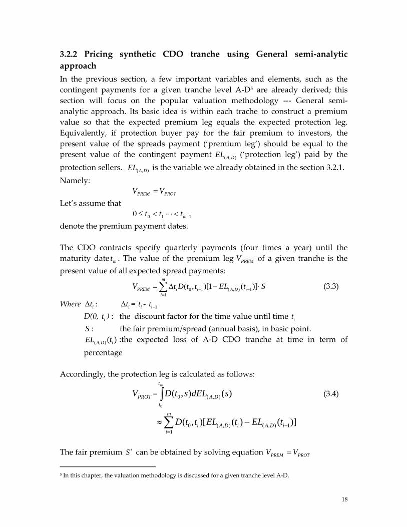
3.2.2 Pricing synthetic CDO tranche using General semi‐analytic approach In the previous section, a few important variables and elements, such as the contingent payments for a given tranche level A‐D5 are already derived; this section will focus on the popular valuation methodology ‐‐‐ General semi‐analytic approach. Its basic idea is within each trache to construct a premium value so that the expected premium leg equals the expected protection leg. Equivalently, if protection buyer pay for the fair premium to investors, the present value of the spreads payment (‘premium leg’) should be equal to the present value of the contingent payment ( , )A DEL (‘protection leg’) paid by the protection sellers. ( , )A DEL is the variable we already obtained in the section 3.2.1. Namely:

PROTPREM VV = Let’s assume that

1100 −<<≤ mttt denote the premium payment dates. The CDO contracts specify quarterly payments (four times a year) until the maturity date . The value of the premium leg of a given tranche is the present value of all expected spread payments:

mt PREMV

PREMV 0 1 ( , ) 11

( , )[1 ( )]m

i i A D ii

t D t t EL t S− −=

= ∆ − ⋅∑ (3.3)

Where : = ‐ it∆ it∆ it 1it −

D(0, ) : the discount factor for the time value until time it it

S : the fair premium/spread (annual basis), in basic point. ( , ) ( )A D iEL t :the expected loss of A‐D CDO tranche at time in term of

percentage Accordingly, the protection leg is calculated as follows:

PROTV = (3.4) 0

0 ( , )( , ) ( )mt

A Dt

D t s dEL s∫

0 ( , ) ( , )1

( , )[ ( ) ( )]m

i A D i A D ii

D t t EL t EL t −=

≈ −∑ 1

The fair premium can be obtained by solving equation S ∗

PROTPREM VV =

5 In this chapter, the valuation methodology is discussed for a given tranche level A‐D.

18

Thus

0 1 ( , ) 1 0 ( , ) ( , ) 11 1

( , )[1 ( )] ( , )[ ( ) ( )]m m

i i A D i i A D i A D ii i

t D t t EL t S D t t EL t EL t− −= =

∆ − ⋅ = −∑ ∑ − (3.5)

0 ( , ) ( , )1

0 1 ( , ) 11

( , )[ ( ) ( )]

( , )[1 ( )]

m

i A D i A D ii

m

i i A D ii

D t t EL t EL tS

t D t t EL t

−∗ =

− −=

−=

∆ −

∑

∑

1

(3.6)

Equation (3.6) is a very compact representation of fair premium . It shows that once we know the expected cumulative loss on a given tranche level in question, for example , the fair premium

S ∗

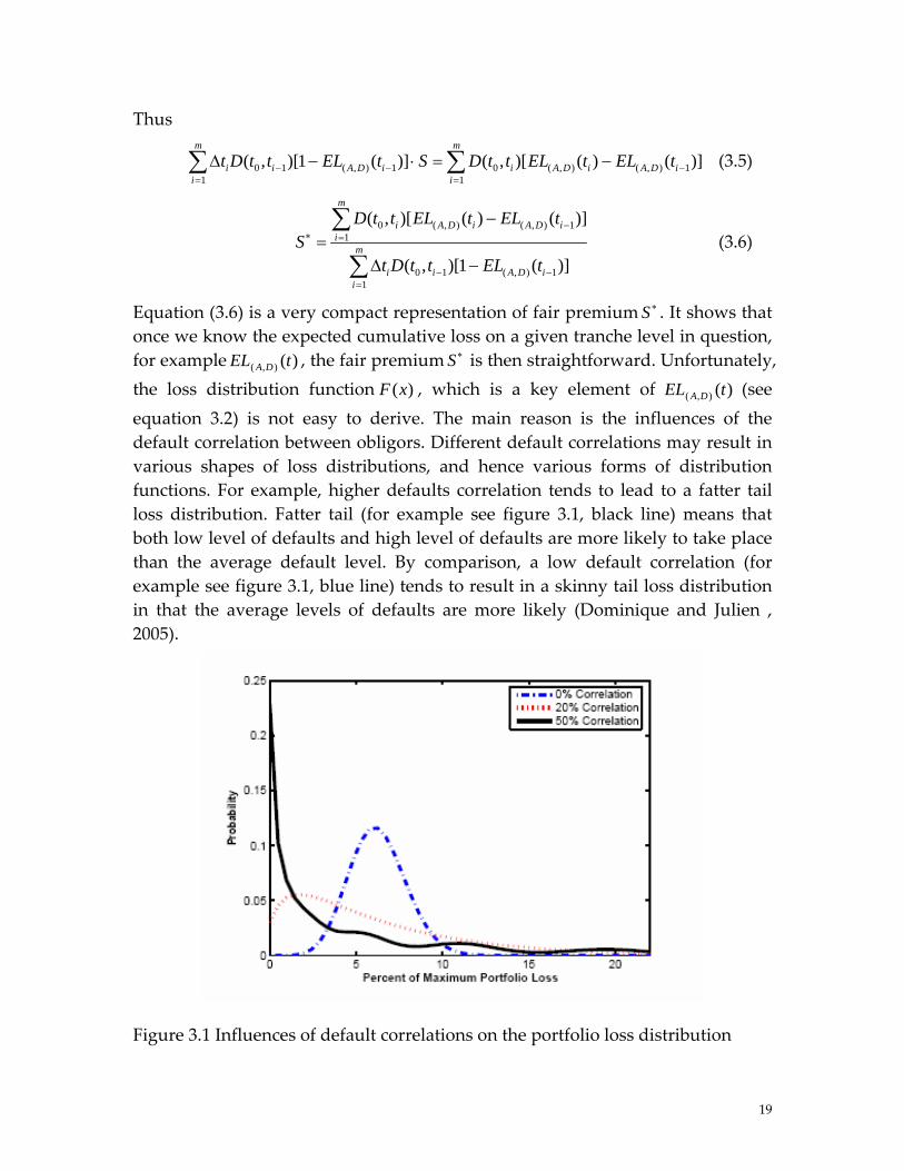
)(),( tEL DA S ∗ is then straightforward. Unfortunately, the loss distribution function , which is a key element of (see equation 3.2) is not easy to derive. The main reason is the influences of the default correlation between obligors. Different default correlations may result in various shapes of loss distributions, and hence various forms of distribution functions. For example, higher defaults correlation tends to lead to a fatter tail loss distribution. Fatter tail (for example see figure 3.1, black line) means that both low level of defaults and high level of defaults are more likely to take place than the average default level. By comparison, a low default correlation (for example see figure 3.1, blue line) tends to result in a skinny tail loss distribution in that the average levels of defaults are more likely (Dominique and Julien , 2005).

)(xF )(),( tEL DA

Figure 3.1 Influences of default correlations on the portfolio loss distribution

19

Source: Dominique and Julien 2005 Consequently, the modeling of default correlation structure plays a crucial role in calculating the loss distribution function, and hence pricing the tranche of a CDO. Note that within the CDO pricing context, we have to not only consider about the joint defaults but also the timing issue (the time to default), because premium payment depends on the outstanding notional which is reduced during the lifetime of the contract if obligors default. The purpose of the next chapter is to present the standard default correlation model and necessary theory which are essential to obtain the loss distribution in a CDO pricing context. Default correlation Default correlation, by definition, is the ‘phenomenon that the likelihood of one obligor defaulting on its debt is affected by whether or not another obligor has defaulted on its debts’. (Douglas Lucas (2004)). For easier understanding, default correlation measures the tendency or the degree of two companies/names to default approximately simultaneously. We have positive /negative default correlation, which respectively means that if one goes to default, others are more /less easy to default.

4. Copula Function and default correlation model (factor copula model) As is shown in the previous chapter, default correlation that determines the loss distribution has been a key element for pricing a CDO tranche. In this chapter, I would like to discuss the default correlations, which are modelled using the factor copula proposed by Li (2000). Before directly discussing the model details, we may first look through the short review of the concept and properties of a copula function, based on which the underlying principle of default correlation model/ factor copula model is built.

4.1 Definition and Basic Properties of Copula Function Let , ,… be m uniform random variables; 1U 2U mU ρ be the correlation parameter. Definition: The joint distribution function 1 2( , , , )mC u u u ρ , denoted with C is called a copula function, if

1 2( , , , )mC u u u ρ = 1 1 2 2,( , m mP U u U u U u )≤ ≤ ≤ For the copula function, an important property is called Sklar’s Theorem, which shows that any multivariate distribution function can be written in the form of a copula function. In addition, the theory clearly reveals that copula may well

F

20

link the marginal probability into a joint distribution. Sklar’s Theorem: If is a joint multivariate distribution function with univariate marginal distribution functions , , , then there exists a copula function such that

1 2( , , )mF x x x

1( )F x 2( )F x ( )mF x

1 2( , , )mC u u u

1 2( , , )mF x x x = 1 2( ( ), ( ), ( ))mC F x F x F xIf each is continuous then C is unique. Thus, copula functions provide a unifying and flexible way to study multivariate distributions.

iF

4.2 Default correlation model (factor copula model) A concise theoretic description of the term’ default correlation’ is presented in the previous section 3.2.2. Now, we start from model’s point of view, there are two types of default correlation models suggested, namely reduced form models and structural models. Duffie and Singleton (1999) and Mertonʹs (1974) already gave the specific description. Considering that the two models are quite computationally time consuming when they are used for pricing products, naturally, we come up with an idea of using the factor copula to model the default correlation. The principal underlied is to make use of the property of the copula function, which is that the factor copula created joint probability distribution for the times to default of many companies/obligors to be constructed from several marginal distributions. This default correlation factor copula model is introduced by Li (2000) and is very popular with the participants in the market. Essentially, the advantage of the copula model lies in its creation of a tractable multivariate joint distribution for a set of variables given the marginal probability distributions for the variables (Hull and White 2004). In the following, the modeling details are introduced. Consider a portfolio of N companies/obligors and assume that the marginal probabilities of defaults are known for each company/obligor. Define:

it : The time of default for the obligor thiQi(t): The cumulative default probability function (cdf) obligor i will

default before time t ; that is, ( tiP t )≤ i.e. the cumulative distribution function of it

21

To generate an one‐factor standard copula model6 for default time , we define a latent random variables

it

ix (1 ≤ i ≤ N) 21i i ix Y iρ ρ ε= + − ⋅ (4.1)

Where the variable ix can be thought of as a default indicator variable for the obligor: the lower the value of the variable, the earlier a default is likely to occur. Each

thi

ix has two stochastic components. The first Y is a common factor which is the same for all ix , while the second iε is an idiosyncratic component affecting only ix . Both the two factors iε and Y have independent zero‐mean unit‐variance distributions. The correlation with the market is represented by iρ and it is in a range of [–1, 1). Since the equation has defined a correlation structure between the ix , dependent on a single common factor Y. The correlation between ix and

jx is ρiρj. Let us look at the general one factor copula model a bit deeper. Under the standard copula factor model framework: 21i i ix Y iρ ρ ε= + − ⋅ ; if we let the iε ’s and Y‘s be standard normal distributions, a Gaussian copula then results. Generally, any distributions can be used for iε ’s and Y‘s providing they are scaled so that they have zero mean and unit variance in order to meet the requirement in the general framework. Each choice of distributions results in a different factor copula to model the default correlation structure, and thus resulting in different methods to derive loss distribution functions for pricing CDO tranche. The choice of the copula models decides the nature of the default dependence structure. Suppose ( )ip y refers to the cumulative default probability, or specifically, the conditional probability of company that go to default before time t, then how to calculate it? How can we derive the formula from the standard one factor copula model framework?

thi

Under the one factor copula model, ix is mapped to using a percentile‐to‐percentile transformation technique. This means that when x

iti is small, the time

before default is also small. For example, the 7% point on the it

ix distribution is mapped to the 7% point on the distribution; and so on. it

6 Here the one‐factor standard copula model is the general copula model framework we use to model the default correlation. All the other copula models including the Gaussian copula model and those introduced in the following chapters are built based on the framework.

22

Define Fi: The cumulative density function of ix i.e. cdf of ix H: The cumulative density function of iε (assuming that the iε

is identically distributed) Then, in general the point is mapped to xxi = tti = where

)]([1 tQFx ii−= K≡ (4.2)

or equivalently )]([1 xFQt ii

−= (4.3)

Note that in some paper, is considered to be a threshold and is often given a notation K or C etc. In the rest of my paper, I use K by default.

)]([1 tQFx ii−=

Observing the copula model shown in equation 4.1, we may find that it essentially defines a default correlation structure between the ’s in the form of it

ix , while maintaining their marginal distributions. In other words, in order to construct the default correlation structure, we do not have to define the correlation structure between the variables of interest (like time to default ’s) directly by using the reduced form models or structural models, which greatly increase the computation complexity. With he help of the factor copula model, typically one factor copula model, we may use mapping technique to map the variables of interest (like ) into other more manageable variables (like

it

it ix ’s) and then define a default correlation structure between those manageable variables. Let H be the cumulative distribution function of iε , we can deduce that

2( | ) ( 1 |i i i iP x x Y y P Y x Y yρ ρ ε< = = + − ⋅ < = ) (4.4)

2( |

1i

i

i

x YP Y )yρερ

−= < =

−

1

2

[ ( )]1

i i ii

i

F Q t YH ρ

ρ

−⎡ ⎤−⎢ ⎥=⎢ ⎥−⎣ ⎦

Therefore, the cumulative probability of the default by time t, conditional on the common factor y is

thi

( | )iP t t Y y< = ( |iP x x Y y= )< =2

( |1

ii

i

x YP )Y yρερ

−= <

−= (4.5)

1

2

[ ( )]1

i i ii

i

F Q t YH ρ

ρ

−⎡ ⎤−⎢ ⎥=⎢ ⎥−⎣ ⎦

= ( )ip y

23

For simplicity, we denote ( |iP t t Y y)< = with ( )ip y . Note that the conditional cumulative probability of one obligor’ default ( )ip y is a key input to calculate the loss distribution. The detailed derivation process of the conditional and unconditional loss distribution functions calculated from ( )ip y , will be presented in the next chapter in loss distribution context.

5. One factor Gaussian copula model Given the standard default correlation models in the previous chapter, I will in the following introduce the current market benchmark model‐One factor Gaussian copula mode. And based on the standard model, the procedures to derive the unconditional /conditional loss distribution functions are addressed.

5.1 One factor Gaussian copula model set up Suppose a portfolio of reference assets consists of N obligors/companies. Recalled that Gaussian copula is actually resulted by defining the iε ’s and Y‘s being standard normal distributions in the standard copula model. In the Gaussian copula model, the latent variable ix is given by

21i i ix Y iρ ρ ε= + − ⋅ 1, 2, ,i N= (5.1) Where ix : latent random variable, following the standard normal

distribution, namely, ix ~ N(0,1); 1, 2, ,i N= X: Gaussian vector, X= ( 1x , 2x ,…, Nx ), following multivariate normal distribution, namely, X~ (0, )NN Σ Y: common factor

iε : Idiosyncratic factor; 1, 2, ,i N=

iρ : Correlation parameter with market, for simplicity, we may assume that iρ = ρ 1, 2, ,i N= Both Y and iε follow the standard normal distributions

Since the default time , , are modelled from the Gaussian vector X,

the default times are given by . In the case of Gaussian copula model (using the same principal we already discussed in the section 4.2)

it 1, 2, ,i = N

]

)]([1 xFQt ii−=

1[ ( )i it Q x−= Φ (5.2) with be the cdf of and be the cumulative normal distribution function of iQ it iΦ

ix ; is just the general inverse function of . Thus 1iQ −

iQ ix is given by 1[ ( )]i ix Q t−= Φ K≡ 1, 2, ,i N= (5.3)

24

The cumulative probability of the default by time t, conditional on the common factor Y is

thi

( | )iP t t Y y< = ( | )iP x x Y y = < = (5.4)

2( |

1i

i

i

x YP Y )yρερ

−= < =

−

1

2

[ ( )]1

i i ii

i

Q t Yρρ

−⎡ ⎤Φ −⎢ ⎥= Φ⎢ ⎥−⎣ ⎦

1, 2, ,i N=

= ( )ip y

5.2 Loss distribution Before discussing the two types of loss distributions (conditional and unconditional), let us look at two assumptions for simplicity. First, we assume that the portfolio is composed of sets of N homogeneous debt instruments, i.e.

iρ = ρ (5.5) =1[ ( )]i iQ t−Φ 1[ ( )]iQ t−Φ iK≡ 1, 2, ,i N=

( )ip y = ( )p yThis assumption ensures that all entities represented in the portfolio have the same default probability over the time period of interest. Second, we assume that each entity represented in the portfolio corresponds to an equal share of the portfolio, or we call it equally weighted homogeneous portfolio. It guarantees the proportional relationship between the number if defaults and the percentage of default related loss. For example, in a portfolio of I reference entities, the probability of m defaults among the reference entities is equivalent to the probability of m/I % default related loss in the portfolio.

5.2.1 Conditional loss probability Considering that the obligors ix in the portfolio is impendent of, yet conditional on the common factor Y, and that only two outcomes are possible for obligors ix , default or not default respectively. Therefore, we may assume the obligors follow a binomial distribution. Given the conditional cumulative probability for obligor

ix ’s default ( )ip y , we may write the conditional loss probability function (conditional probability density function) that totally i companies go to default by applying the binomial distribution

( | ) ( ) (1 ( ))i Ni i

NP X i Y y p y p y

ii−⎛ ⎞

= = = −⎜ ⎟⎝ ⎠

(5.6)

25

( ) (1 ( ))i NNp y p y

ii−⎛ ⎞

= −⎜ ⎟⎝ ⎠

With

( )p y =2

( )1

ix YP ρε

ρ−

<−

=1

2

[ ( )]1iQ t Yρ

ρ

−⎡ ⎤Φ −Φ⎢ ⎥

−⎢ ⎥⎣ ⎦

Ni⎛ ⎞⎜ ⎟⎝ ⎠

= !!( )!

Ni N i−

Note that ( )ip y means the conditional probability of obligor ix ’s default and it has already been derived in equation (5.4). Under the homogeneous portfolio assumption, the probability of i out of N entities which go to default is equal to

the probability of the loss being the amount = nL nL (1 )i A RN⋅ −

5.2.2 Unconditional loss distributions To derive the expression for the unconditional loss probability, we just need to do integration over the common factor Y

( ) ( | ) ( )P X i P X i Y y y dyφ+∞

−∞

= = = =∫ (5.7)

Where ( )φ ⋅ is the probability density function of standard normal distribution, because Y is following standard normal distribution. Substituting equation 5.6 and 5.4 in equation 5.7, we obtain the following expression for the unconditional probability of i defaults in the portfolio

( ) ( ) (1 ( )) ( )i N iNP X i p y p y y dy

iφ

+∞−

−∞

⎛ ⎞= = −⎜ ⎟

⎝ ⎠∫ (5.8)

1 1

2 2

[ ( )] [ ( )]! 1 (!( )! 1 1

i N

i i i i

i i

Q t Y Q t YN y dyi N i

ρ ρ φρ ρ

−+∞ − −

−∞

⎧ ⎫ ⎧ ⎫⎡ ⎤ ⎡ ⎤Φ − Φ −⎪ ⎪ ⎪ ⎪⎢ ⎥ ⎢ ⎥= ⋅ Φ −Φ⎨ ⎬ ⎨ ⎬− ⎢ ⎥ ⎢ ⎥− −⎪ ⎪ ⎪ ⎪⎣ ⎦ ⎣ ⎦⎩ ⎭ ⎩ ⎭∫ )

i

)

Therefore, the unconditional loss distribution function of defaults

0

( ) (m

i

P X m P X i=

≤ = =∑ (5.9)

1 1

2 20

[ ( )] [ ( )]! 1 (!( )! 1 1

i Nm

i i i i

i i i

Q t Y Q t YN y dyi N i

ρ ρ φρ ρ

−+∞ − −

= −∞

⎧ ⎫ ⎧ ⎫⎡ ⎤ ⎡ ⎤Φ − Φ −⎪ ⎪ ⎪ ⎪⎢ ⎥ ⎢ ⎥= ⋅ Φ −Φ⎨ ⎬ ⎨ ⎬− ⎢ ⎥ ⎢ ⎥− −⎪ ⎪ ⎪ ⎪⎣ ⎦ ⎣ ⎦⎩ ⎭ ⎩ ⎭∑ ∫ )

i

Note that for Gaussian copula model, by assumption, iρ = ρ holds for all the obligors.

26

5.3 The large portfolio approximation for the one factor model The calculation of the unconditional loss distribution in equation (5.9) is computationally trivial, especially for a very large N. In order to overcome this problem, Vasicek (1987) proposed the large portfolio approximation approach, which is a convenient and efficient way for approximation when the N tends to be∞ . Let x be the fraction of defaulted entities in the portfolio, then

( ) ( )NF x p X x= ≤ (5.10)

1 1

2 20

! [ ( )] [ ( )]lim 1 ( )!( )! 1 1

i NNx

i i i i

N i i i

N Q t Y Q t Y y dyi N i

ρ ρ φρ ρ

−+∞ − −

→∞= −∞

⎧ ⎫ ⎧ ⎫⎡ ⎤ ⎡ ⎤Φ − Φ −⎪ ⎪ ⎪ ⎪⎢ ⎥ ⎢ ⎥= ⋅ Φ −Φ⎨ ⎬ ⎨ ⎬− ⎢ ⎥ ⎢ ⎥− −⎪ ⎪ ⎪ ⎪⎣ ⎦ ⎣ ⎦⎩ ⎭ ⎩ ⎭

∑ ∫i

Define = , and 1[ ( )]iQ t−Φ iK21

i i

i

K Yρρ

⎡ ⎤−⎢ ⎥Φ⎢ ⎥−⎣ ⎦

= with im iρ = ρ holds for all the

obligors, we have

Y=11 ( )im Kρρ

−− Φ − i (5.11)

Hence ( ) ( )NF x p X x= ≤ (5.12)

1

0

1 ( )!lim 1 [ ] !( )!

Nxi N i i i

i iN i

m KN m m di N i

ρρ

+∞ −−

→∞= −∞

− Φ −= ⋅ − Φ

−∑ ∫

Since

0

0 if x!lim 1 1 otherwise!( )!

Nxi N i i

i iN i

mN m mi N i

+∞−

→∞= −∞

≤⎧⋅ − = ⎨

− ⎩∑ ∫ (5.13)

The cumulative distribution function of loss of large portfolio is given by ( ) ( )F x p X x= ≤

11 ( )= [ ] ix Kρρ

−− Φ −Φ (5.14)

It is easy to see the expression of loss distribution function using large portfolio approach displayed in equation (5.14) is much compacter and handier than the one shown in equation (5.9). With the above expression, we may easily calculate the expected tranche losses and then the corresponding CDO tranche premium.

( )F x

27

5.4 Evaluation of the Gaussian copula approach Gaussian factor copula model has been widespread applied for the valuation of types of instruments and already become a current industry standard. Its attractiveness of pricing CDOs is evident due to simplicity and straightforward application, which merely requires simple and fast numerical integration techniques (Guegan, Dominique and Houdain, Julien, 2005). However, it is argued that the assumptions for this model are too strong. For example, the model assumes the correlation parameter with market (compound implied correlation) iρ = ρ holds for all the obligors, recovery rate is also constant etc. Recently many researches reveal that several serious drawbacks do exist in Gaussian copula model, which tend to result in mispricing the tranche spreads. Thus it might not be an ideal method to price the tranche of CDO. In the following, two categories of the shortcomings are discussed.

5.4.1 Correlation structure Under the Gaussian copula model, a flat correlation structure is drawn due to the constant correlation parameter iρ assumption. But a flat correlation structure is not sufficient to reflex the heterogeneity of the underlying assets (e.g. ). Accordingly, since one single number

ixρρ couldn’t explain well the complex

relationship between the default times of different assets like thus it is obviously not appropriate to use Gaussian copula model, especially its constant implied compound correlations

ji xx

ρ of traded tranches. Implied correlation Mashal et al. (2004) define the implied correlation (the correlation parameter iρ ) of a tranche as the uniform asset correlation number that makes the fair or theoretical value of a tranche equal to its market quote. In other words, Hull and White (2004) for example define the implied correlation for a tranche as the correlation that causes the value of the tranche to be zero. Implied correlations do exist within each tranche yet generally not uniquely defined. In addition, tranche spreads are not necessarily monotone in correlation. Therefore, we may observe the market prices that may not be attainable by just one choice of constant correlation parameter as Gaussian copula does (Svenja Hager and Rainer Schöbel, 2005).

28

Tranche [0,3] [3,6] [6,9] [9,12] Market quote 27.6% 1.68% 0.7% 0.43% Gauss ρ =21.9% 27.6% 2.95% 1.05% 0.42% Gauss ρ =4.2% 43.1% 1.68% 0.1% 0.005% Gauss ρ =87.9% ‐‐‐‐‐‐‐ 1.68% 1.35% 1.14% Gauss ρ 14.8% 33.2% 2.68% 0.7% 0.2% Gauss ρ =22.3% 27.3% 2.96% 1.07% 0.43% Gauss ρ =30.5% 21.6% 3.05% 1.35% 0.67%

Table 5.1 Implied correlations from Gaussian copula The table 5.1 displays the implied correlations parameters from the Gaussian copula, and we may observe the ρ does exist in every tranche and also not unique, such as in the tranche [3, 6], ρ =4.2% and ρ =87.9% result in the same premium 1.68%.

5.4.2 Correlation smile As the market quotes on CDOs become more readily available, researchers are able to calibrate their model parameters to those real market quotes. Under the chosen model, using the correlation matrix, we may compute the spreads for each traches. And from these spreads the implied correlation can be derived. In the real market, quotations available indicate that different tranches on the same underlying portfolio trade at different implied correlations, which in the following figure 5.1 resembles a smile skew, called correlation smile. However, it is not the case under the standard Gaussian model, which expects the compound correlation being equal for every single tranche and thus the Gaussian copula model doesn’t lead to a smile skew yet a flat structure. From the table 5.1, we may also observe the implied correlations for each tranche are not the same. Such problems are mainly due to the simplifying assumptions that the correlations as well as the recovery rates and CDS spreads are constant and equal for all obligors. The correlation smile in Figure 5.1 plot below shows a lower default time correlation on the mezzanine tranche than on the equity and senior tranches. So, we can conclude that the degree of default clustering assumed by the market appears to be higher for the equity and senior tranches. Quotations available in the market indicate that different tranches on the same underlying portfolio trade at different implied correlations. It might be that the Gaussian copula model could not accurately reflect the joint distribution of default times.

29

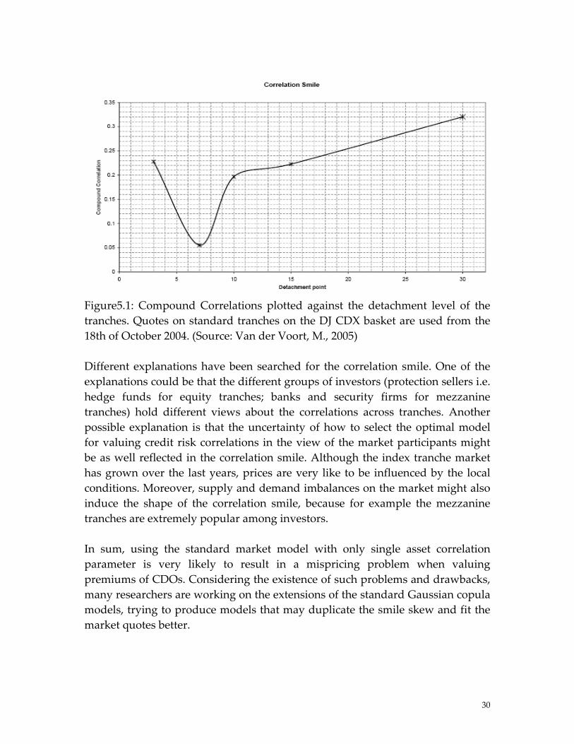
Figure5.1: Compound Correlations plotted against the detachment level of the tranches. Quotes on standard tranches on the DJ CDX basket are used from the 18th of October 2004. (Source: Van der Voort, M., 2005) Different explanations have been searched for the correlation smile. One of the explanations could be that the different groups of investors (protection sellers i.e. hedge funds for equity tranches; banks and security firms for mezzanine tranches) hold different views about the correlations across tranches. Another possible explanation is that the uncertainty of how to select the optimal model for valuing credit risk correlations in the view of the market participants might be as well reflected in the correlation smile. Although the index tranche market has grown over the last years, prices are very like to be influenced by the local conditions. Moreover, supply and demand imbalances on the market might also induce the shape of the correlation smile, because for example the mezzanine tranches are extremely popular among investors. In sum, using the standard market model with only single asset correlation parameter is very likely to result in a mispricing problem when valuing premiums of CDOs. Considering the existence of such problems and drawbacks, many researchers are working on the extensions of the standard Gaussian copula models, trying to produce models that may duplicate the smile skew and fit the market quotes better.

30

6. Extensions to the Gaussian model and its comparisons There has been much interest recently in simple extensions of the Gaussian one‐factor model in order to match the ʺcorrelation smileʺ in the CDO market. Gregory and Laurent (2004) propose a correlation structure built from groups specifying intra and inter group correlation coefficients and they introduce some dependence between recovery rates and defaults. Hull and White (2005) recommend the use of a double Student‐t one‐factor model. Andersen and Sidenius (2005) introduce random recovery rates and random factor loadings in the model. Burtschell, Gregory and Laurent (2005) propose a comparative analysis of the previous CDO pricing models and illustrate the fact that these models should be improved. In the following, I will review some typical extensive models in details.

6.1 Student t copula model In student t approach, the vector X= ( 1x , 2x ,…, Nx ) follows a student t distribution with u degrees of freedom. For simplicity, we consider the symmetric situation

21i i ix w Y w iρ ρ ε= ⋅ ⋅ + − ⋅ ⋅ (6.1) 2( 1i iw Y )iρ ρ ε= + − ⋅ 1, 2, ,i N=

Where Y, iε : independent Gaussian random variables W: has inverse Gamma distribution with the parameter u/2

(or 2~ nuw

χ ) and w is independent of ix

Cov( ,i jx x )= ( )2 i j

uu

ρ ρ−

(u>2) (6.2)

We denote by T the cdf of standard univariate student t distribution, thus the default time t is given by

1[ ( )]i i i it Q T x−= (6.3) Equivalently

1[ ( )]i i i i ix T Q t K−= ≡ (6.4) Accordingly, the cumulative probability of the obligor‘s default by time t, conditional on the common factor Y is

thi

( ) ( | )i iP y P t t Y y= < = ( |iP x x Y y= < = )

2( 1 |i i i iP Y W W K Y yρ ρ ε= + − ⋅ < )=

31

2( )

1i i

i

i

K Y WPW

ρερ

−= <

−

2(

1i i

i

K Y WW

ρ

ρ

−= Φ

−) (6.5)

6.2 Double t copula model Define latent random vector X= ( 1x , 2x ,…, Nx ), which modelled the default times , it 1, 2, ,i N=

1/ 2 22 2( ) 1 ( )i i iux Y

u u iuρ ρ−

= + − ε−⋅ (6.6)

Where Y, iε : both follow student t distribution with degree of freedom and u u respectively

iρ : iρ ≥0 It is noted that student t distributions are not stable under convolution, though two main factors Y, iε both follow t‐distribution, ix didn’t. Thus the copula associates with ( 1x , 2x ,…, Nx ) is not a student copula , which distinguish itself with student t copula model. Simply, default time is given by 1[ ( )]i i i it Q F x−=Equivalently

1[ ( )]i i i i ix F Q t K−= ≡ (6.7) Where : the cumulative distribution function of t iQ i

: the cumulative distribution function of iF ix Accordingly, the cumulative probability of the obligor‘s default by time t, conditional on the common factor Y is

thi

( ) ( | )i iP y P t t Y y= < = (6.8) ( |iP x x Y y= < = )

1/ 2 22 2(( ) 1 ( ) | )i i i iu uP Y K Y

u uρ ρ ε− −

= + − ⋅ < y=

1/ 2

2

2( )( )21 ( )

i i

i

i

uK YuP u

u

ρε

ρ

−−

= <−

−

32

1/ 2

2

2( )( )21 ( )

i i

i

i

uK YuT u

u

ρ

ρ

−−

=−

−

6.3 Clayton copula model Define a random variable L, following a standard Gamma distribution with

shape parameter 1θ where 0θ > , i.e. 1~ ( )L

θΓ .

The probability of density function of L is given by (1 ) /1( ) e1( )

xf x x θ θ

θ

− −=Γ

; (6.9) 0x >

We denote by ψ the laplace transformation of L

1/

0

( ) ( ) (1 )yxy f x e dx y θψ+∞

− −= = +∫ (6.10)

Let be independent uniform random variables, and independent of L 1 2, , Nu u uThe Clayton factor model is written as

ln( ii

ux )L

ψ= − (6.11)

Then the default time are given by it1( )i i it Q x−=

Or equivalently ( )i i ix Q t= (6.12)

The cumulative probability of the obligor‘s default by time t, conditional on the common factor Y is

thi

( ) ( | )i iP l P x x L l= < = (6.13)

= ln( ( ) ( ) | )ii

uP Q t L lL

ψ − < =

exp( (1 ( ) )il Q t θ−= ⋅ − Gregory & Laurent [2003] and Laurent & Gregory [2003] have been considering this model in a credit risk context.

6.4 Normal inverse Gaussian model Normal inverse Gaussian distribution (NIG) is a special case of the group of generalized hyperbolic distributions (Barndorff‐Nielsen). They are stable under convolution in certain conditions and the cumulative density function (cdf),

33

probability density function and inverse distribution function can still be computed sufficiently fast. Kalemanova et al has applied the normal inverse Gaussian models to the CDO pricing recently and proved a good fit to market data.

6.4.1 Definition and properties of the NIG distribution The normal inverse Gaussian distribution is a mixture of normal and inverse Gaussian distributions. Definition: a Non‐negative random variable Y has inverse Gaussian (IG) distribution with parameters α > 0 and β > 0, i.e. ~ ( , ,y IG y)α β , if its density function satisfy

23 / 2 ( )exp( ) if y>0

2( ; , ) 2 0 otherwise

IG

yyyf y

α α ββα β πβ

−⎧ − −⎪= ⎨⎪⎩

(6.14)

Definition: A random variable X follows a normal inverse Gaussian (NIG) distribution with parametersα , β , ,η γ , i.e. ~ ( , , , , )X NIG xα β η γ , if

X|(Y=y)~ ( , )N y yη β+ (6.15)

and 2~ ( ,Y IG )γλ λ with 2 2:λ α β= − satisfy constraints

0 | |β α≤ < and 0η > Denote by ( , , , , )NIGf x α β η γ , ( , , , , )NIGF x α β η γ the density function and the cumulative distribution function of ~ ( , , , , )X NIG xα β η γ respectively. We have

( , , , , )NIGf x α β η γ 212 2

exp( ( )) ( (( )

x K xx

2) )γλ γλ β η α γ ηπ γ η

+ −= ⋅

− −− − (6.16)

where 11

0

1 1( ) : exp( ( )2 2

K w w t t dt∞

−= − +∫ is the modified Bessel function of the third

Kind. The density function relies on four parametersα , β , ,η γ , with α related to steepness, β influencing the symmetry, and ,η γ respectively to location and scale. Next I will introduce two important properties of NIG distribution. One is called “scaling property”, which is given by

~ ( , , , , ) ~ ( , , , )X NIG x cX NIG c cc cα βα β η γ η γ⇒ (6.17)

where c is a constant.

34

The second property is about NIG distribution’s stability under the convolution situation. Let X, Y, T be independent random variables

1 1~ ( , , , , )X NIG xα β η γ 2 2~ ( , , , , )IG y; Y N α β η γ)

1 2 2 1~ ( , , , ,T X Y NIG tα β η η γ γ⇒ = + + + (6.18) The mean and variance of a random variable ~ ( , , , , )X NIG xα β η γ are given by

22)(

βαβγη−

+=xE

22

2

)(βα

γα−

=xVar

1( ) 3( )( )Skew x βα ηγ

=

2 1( ) 3[1 4( ) ]( )Kurt x βα ηγ

= +

6.4.2 Normal inverse model set up

iiii Yx ερρ ⋅−+= 21 where iρ : constant correlation parameter, Ni ,...2,1= iε ,Y: independent NIG random variables satisfy

),,,(~22α

βααββα−

−NIGY

)1

,1

,1

,,1

(~2

22

222

αρρ

βααβ

ρρ

βρρ

αρρ

εi

i

i

i

i

i

i

ii NIG

−

−

−−−−

Note that the NIG implied common factor Y is different from Gaussian common factor7. Using the two properties we discussed in 6.5.1, we get

),1,,(~22

iiiii NIGx

ρα

βααβ

ρρβ

ρα

−− (6.19)

For simplicity, we denote probability distribution function of , ix Ni ,...2,1=

),1,,,(22

iiiiNIG xF

ρα

βααβ

ρρβ

ρα

−− with )(

)1(xF

iNIG

ρ

. Hence, iε has distribution

function of )()

1(

2 xFi

iNIGρρ−

.

The default time is given by

7 For a more detailed description, see Guegan, Dominique and Houdain, Julien, 2005.

35

)]([)1(

1iNIGii xFQt

iρ

−=

equivalently )]([1

)1(tQFx i

iNIG

−=ρ

iK≡ (6.19)

then the conditional probability of the obligor/company that defaults before time t is given by

thi

)()|( ypYttp ii =<

)|1( 2 yYKYp iii =<−+= ρρ

)1

(2

i

iii

YKpρ

ρε−

−<=

)1

(2

)1

(2

i

ii

NIG

YKFi

i ρ

ρ

ρρ −

−=

− (6.20)

The large portfolio approximation is given by (according to the section 5.3)

( ) ( )F x P X x∞ = ≤

2

2 1

1( )

(1)

( 1 ) ( )

[ ]i

i

i iNIG

NIGi

F x

Fρ

ρ

ρ

ρ

−

−− −

=

K

(6.21)

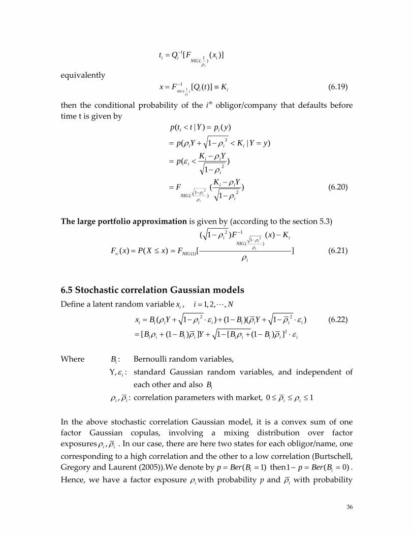
6.5 Stochastic correlation Gaussian models Define a latent random variable ix , 1, 2, ,i N=

2 2( 1 ) (1 )( 1i i i i i i i i ix B Y B Y )ρ ρ ε ρ ρ ε= + − ⋅ + − + − ⋅ (6.22) 2[ (1 ) ] 1 [ (1 ) ]i i i i i i i i iB B Y B Bρ ρ ρ ρ= + − + − + − ⋅ε

Where iB : Bernoulli random variables,

Y, iε : standard Gaussian random variables, and independent of each other and also iB

iρ , iρ : correlation parameters with market, 0 1i iρ ρ≤ ≤ ≤

In the above stochastic correlation Gaussian model, it is a convex sum of one factor Gaussian copulas, involving a mixing distribution over factor exposures iρ , iρ . In our case, there are here two states for each obligor/name, one corresponding to a high correlation and the other to a low correlation (Burtschell, Gregory and Laurent (2005)).We denote by ( 1ip Ber B )= = then1 ( . Hence, we have a factor exposure

0)ip Ber B− = =

iρ with probability p and iρ with probability

36

(1‐ p). In addition, the marginal distributions of ix are Gaussians. The default time is given by

1[ ( )i i i it Q x−= Φ ] Note that the default times are independent conditionally on Y, then, the conditional cumulative default probabilities is

( ) ( | )i iP y P x x Y y= < = (6.23)

1 1

2 2

[ ( )] [ ( )](1 )

1 1i i i i

i i

Q t Y Q t Yp p

ρ ρ

ρ ρ

− −⎡ ⎤ ⎡ ⎤Φ − Φ −⎢ ⎥ ⎢ ⎥= ⋅Φ + − ⋅Φ⎢ ⎥ ⎢ ⎥− −⎣ ⎦ ⎣ ⎦

6.6 Random factor loading (RFL) model The random factor loading model is introduced by Andersen and Sidenius. Its underlying idea is to make factor loadings, basing on the factor models, being functions of the system/common factors themselves. Interpreting the systematic factor as the ‘state of market’ with its value being high in good time and lower in the bad time, the RFL model may mimic the well‐known empirical effect that equity (and thereby asset) correlations are higher in a bear market than in a bull market (Andersen, L. and Sidenius, J. (2004))

6.6.1 Model set up ( )i i i i ix Y Y v mρ ε= + ⋅ + (6.24)

Where iρ : factor loading, with d‐dimension Y, iε : Y is a d‐dimension variable i.e. Y = ( ,…, ) ,

Both are independent random variables with zero mean and unit variance

1Y dY 1, 2, ,i N=

iv , : they are set so that im ix has zero mean and unit variance distribution

Let be the cdf of Y, then , are given by YF iv im

iv = 1 ( ( ) ) 21 ( ( ) ) ( )d

Yi i

R

Y Y dF Y mρiVar Y Yρ− = − +∫ (6.25)

im [ ( ) ]iE Y Yρ= − ( ) ( )d

Yi

R

Y YdF Yρ= − ∫ (6.26)

The default time is given by it1[ ( )x

i i i it Q F x−= ] Equivalently, we get

[ ( )]xi i i ix F Q t−= = (6.27) iK

37

Where xiF is distribution function of ix , is ’s, is a threshold value. iQ it iK

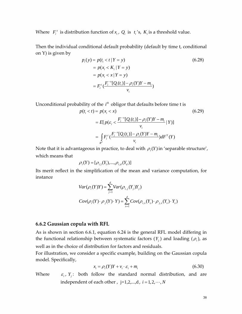
Then the individual conditional default probability (default by time t, conditional on Y) is given by

( ) ( | )i ip y p t t Y y= < = (6.28) ( |i i )p x K Y y= < = ( |i )p x x Y y= < =

[ ( )] ( )( )x

i i i i ii

i

F Q t Y Y mFv

ε ρ− − −=

Unconditional probability of the obligor that defaults before time t is thi

( ) (i i )p t t p x x< = < (6.29)

[ ( )] ( )[ ( | )]x

i i i i ii

i

F Q t Y Y mE p Yvρε

− − −= <

[ ( )] ( )( )d

xYi i i i i

iiR

F Q t Y Y m ( )F dF Yv

ε ρ− − −= ∫

Note that it is advantageous in practice, to deal with ( )i Yρ in ‘separable structure’, which means that

( )i Yρ ,1 1 ,[ ( ),..., ( )]i i dY Ydρ ρ=

Its merit reflect in the simplification of the mean and variance computation, for instance

,1

( ( ) ) ( ( ) )d

i ij

Var Y Y Var Y Yρ ρ=

=∑ j j j

s

, ,1

( ( ) ( ) ) ( ( ) ( ) )d

i j i s s j s ss

Cov Y Y Y Cov Y Y Yρ ρ ρ ρ=

⋅ ⋅ = ⋅ ⋅∑

6.6.2 Gaussian copula with RFL As is shown in section 6.6.1, equation 6.24 is the general RFL model differing in the functional relationship between systematic factors ( jY ) and loading ( iρ ), as well as in the choice of distribution for factors and residuals. For illustration, we consider a specific example, building on the Gaussian copula model. Specifically,

( )i i i i ix Y Y v mρ ε= + ⋅ + (6.30) Where iε , jY : both follow the standard normal distribution, and are

independent of each other , , j=1,2,...,d 1, 2, ,i N=

38

,i jρ : Often written as iρ for simplicity and it is the factor loading, N*d matrix. We define it to be a two point distribution, which is given by

j,

if Y( )

otherwiseij ij

i j jij

aY

b

θρ

≤⎧⎪= ⎨⎪⎩

With and , both matrix being positive constant, ija ijb ij Rθ ∈ , : the same formula as the general one iv im For better understanding, we may think of that as a regime‐switching model where the loading takes the value with probabilityija ( )ijθΦ , and value with a probability [1‐

ijb

( )ijθΦ ]. If > , the factor loadings decrease in ija ijb jY and thus, intuitively, the asset values couple more strongly to “the economy” in bad times than in good times. By using the Gaussian copula with RFL model, we may not only crudely mimic an empirical dependence of correlation on the broad market condition, but also generate a base correlation skew when > . To elaborate, consider in the view of senior tranche investor. This investor will only experience losses on his position when several names/companies default together (or consider it to be extreme loss outcomes‐‐‐both very high and very low levels of defaults). Generally, high values of correlation parameters/factor loadings tend to result in fatter tails of distribution, which mean the extreme loss outcomes. In our case, the systematic factor Y should be low, and then the factor loadings will be high, making it appear to senior investor that correlation is high. For the equity tranche holder on the other hand, who is likely to bear losses even in scenarios where systematic factor Y is not low, the effective factor loading will appear as a weighted average between and . Hence the world will thus look as if correlations are of average magnitude to them. Evidently, if = , it is back to the constant factor loading of Gaussian case.

ija ijb

ija ijb

ija ijb

Calculation of and iv imIn the Gaussian copula with RFL model: , are set so that iv im ix has zero mean and unit variance distribution.

im [ ( ) ]iE Y Yρ= −1

[ ( ) (d

ij ij ij ijj

a b )]ϕ θ ϕ θ=

= − − +∑ (6.31)

iv = 1 ( ( ) )iVar Y Yρ−1

1d

ijj

V=

= −∑ (6.32)

39

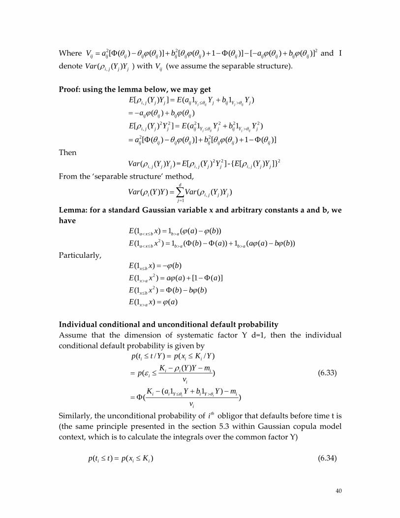
Where and I denote

2 2[ ( ) ( )] [ ( ) 1 ( )] [ ( ) ( )]ij ij ij ij ij ij ij ij ij ij ij ij ijV a b a bθ θ ϕ θ θ ϕ θ θ ϕ θ ϕ θ= Φ − + + −Φ − − + 2

,( ( )i j j jVar Y Yρ ) with (we assume the separable structure). ijV

Proof: using the lemma below, we may get

,[ ( ) ] ( 1 1 )j ij j iji j j j ij Y j ij Y jE Y Y E a Y b Yθ θρ ≤ >= +

( ) ( )ij ij ij ija bϕ θ ϕ θ= − + 2 2 2 2 2 2

,[ ( ) ] ( 1 1j ij j iji j j j ij Y j ij Y jE Y Y E a Y b Yθ θρ ≤ >= + )

2 2[ ( ) ( )] [ ( ) 1 ( )]ij ij ij ij ij ij ij ija bθ θ ϕ θ θ ϕ θ θ= Φ − + + −Φ Then

,( ( ) )i j j jVar Y Yρ = ‐ 2 2,[ ( )i j j jE Y Yρ 2

,[ ( ) ]i j j jE Y Yρ

j j j

]From the ‘separable structure’ method,

,1

( ( ) ) ( ( ) )d

i ij

Var Y Y Var Y Yρ ρ=

=∑

Lemma: for a standard Gaussian variable x and arbitrary constants a and b, we have

(1 ) 1 ( ( ) ( ))a x b b aE x a bϕ ϕ< ≤ >= − 2(1 ) 1 ( ( ) ( )) 1 ( ( ) ( ))a x b b a b aE x b a a a bϕ ϕ< ≤ > >= Φ −Φ + − b

Particularly, (1 ) ( )x bE x bϕ≤ = −

2(1 ) ( ) [1 ( )]x aE x a a aϕ> = + − Φ 2(1 ) ( ) ( )x bE x b bϕ≤ = Φ − b

(1 ) ( )x aE x aϕ> = Individual conditional and unconditional default probability Assume that the dimension of systematic factor Y d=1, then the individual conditional default probability is given by

( / ) ( / )( )(

( 1 1 )( )i i

i i i

i i ii

i

i i Y i Y i

i

p t t Y p x K YK Y Y mp

vK a Y b Y m

vθ θ

ρε

≤ >

≤ = ≤

− −= ≤

− + −= Φ

) (6.33)

Similarly, the unconditional probability of obligor that defaults before time t is (the same principle presented in the section 5.3 within Gaussian copula model context, which is to calculate the integrals over the common factor Y)

thi

)()( iii Kxpttp ≤=≤ (6.34)

40

);,()();,(222222222222

ii

ii

ii

ii

ii

ii

ii

ii

ii

ii

bvb

bvmK

bvmK

ava

avmK

++

−Φ−

+

−Φ+

++

−Φ= θθ

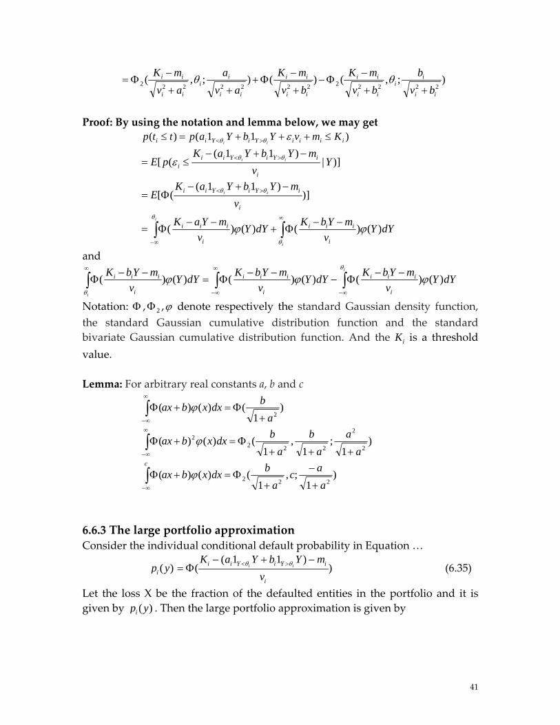
Proof: By using the notation and lemma below, we may get

)11()( iiiiYiYii KmvYbYapttpii

≤+++=≤ >< εθθ

)]|)11(

([ Yv

mYbYaKpE

i

iYiYiii

ii−+−

≤= >< θθε

)])11(

([i

iYiYii

vmYbYaK

E ii−+−

Φ= >< θθ

dYYv

mYbKdYYv

mYaK

i

iii

i

iii

i

i

)()()()( ϕϕθ

θ −−Φ+

−−Φ= ∫∫

∞

∞−

and

dYYv

mYbKdYYv

mYbKdYYv

mYbK

i

iii

i

iii

i

iiii

i

)()()()()()( ϕϕϕθ

θ

−−Φ−

−−Φ=

−−Φ ∫∫∫

∞−

∞

∞−

∞

Notation: Φ , ,2Φ ϕ denote respectively the standard Gaussian density function, the standard Gaussian cumulative distribution function and the standard bivariate Gaussian cumulative distribution function. And the is a threshold value.

iK

Lemma: For arbitrary real constants a, b and c

)1

()()(2a

bdxxbax+

Φ=+Φ∫∞

∞−

ϕ

)1

;1

,1

()()(2

2

2222

aa

ab

abdxxbax

+++Φ=+Φ∫

∞

∞−

ϕ

)1

;,1

()()(222

aac

abdxxbax

c

+

−

+Φ=+Φ∫

∞−

ϕ

6.6.3 The large portfolio approximation Consider the individual conditional default probability in Equation …

( )ip y( 1 1 )

( i ii i Y i Y i

i

K a Y b Y mv

θ θ< >− + −= Φ ) (6.35)

Let the loss X be the fraction of the defaulted entities in the portfolio and it is given by ( )ip y . Then the large portfolio approximation is given by

41

1

1

lim 1 ( ) lim ( )

( ( ) )( )[ (

( ( ) ( ) ))

NN N

i

i i i

i

i i i

F x p X x

P p y xK Y Y mP x

v

P Y Y K v x m

ρ

ρ

→∞ →∞

−

−

− = ≥

= ≥− −

= ≥

= ≤ − Φ −

)]

i

Φ

i

(6.36)

For simplicity, we denote 1( ) ( )i ix K v x m−Ω ≡ − Φ − , then

lim ( )N

p X x→∞

≥

( )

[ ( ) ( ), ] [ ( ) ( ), ][ ( ), ] [ ( ), ]

( ) ( )1 [min( , )] 1 [ ( ) ( )]i

i

i i i

i i i i

i x ii ia

P Y Y x Y P Y Y x YP aY x Y P bY x Y

x xa bθ

iρ θ ρ θθ θ

θ θΩ>

= ≤ Ω ≤ + ≤ Ω= ≤ Ω ≤ + ≤ Ω >

⎛ ⎞Ω Ω= − Φ + Φ −Φ⎜ ⎟⎜ ⎟

⎝ ⎠

>

≥

Therefore, the cumulative loss distribution for the random loading model is given by

( )F x∞ =1 l (6.37) im ( )N

p X x→∞

−

( )( ) ( )1 [min( , )] 1 [ ( ) ( )]

ii

i x ii ia

x xa bθ

θ θΩ>

⎛ ⎞Ω Ω= − Φ + Φ −Φ⎜ ⎟⎜ ⎟

⎝ ⎠

6.7 Perfect copula Implied copula approach or so called ‘perfect copula’ is proposed by Hull and White 2006. This is a ‘perfect model ‘ in terms of its exact fit to the market quotes.

6.7.1 Implied hazard rate paths

Before presenting the specific approach, let us recall the one‐factor copula and its implied hazard rate paths. In the chapter 4.2, we derive that

2( | ) ( 1 |i i i iP x x Y y P Y x Y yρ ρ ε< = = + − ⋅ < = )

1

2

[ ( )]1

i i ii

i

F Q t YH ρ

ρ

−⎡ ⎤−⎢ ⎥=⎢ ⎥−⎣ ⎦

(4.4)

where is the cumulative distribution function of iH iε .

Therefore, the cumulative probability of the default by time t, conditional on the common factor y is

thi

42

( | )iP t t Y y< = ( |iP x x Y y= )< =2

( |1

ii

i

x YP )Y yρερ

−= <

−=

1

2

[ ( )]1

i i ii

i

F Q t YH ρ

ρ

−⎡ ⎤−⎢ ⎥=⎢ ⎥−⎣ ⎦

= ( )ip y (4.5) Now, instead of formulating the models in terms of conditional cdf ( )ip y , we may use conditional hazard rate. Let )|( ytiλ be the hazard rate at time t conditional on common factor Y for obligor i. Then we model the cumulative default probability by assuming that defaults occur according to Poisson process. The relationship between the hazard rate and the cumulative default probability is then

])|(exp[1)(0∫−−=t

ii dsysyp λ

or equivalently

)(1)()|( yp

dtydpyti

ii −=λ (6. 38)

The equation (6. 38) in conjunction with (4.5) can be used to calculate the hazard rate as a function of time t conditional on Y. thus that function is denoted by hazard rate path. The probability that iλ = )|( ytiλ is iβ . The calibration problem is to choose the appropriate set of iλ and its corresponding iβ . In the Hull and White 2006, the details about the specific method for calculating iλ and iβ as well as some discussions of the hazard rate path on different models are presented.

6.7.2 Implied copula approach In the previous section in the equation (6. 38), we have seen that the hazard rate paths of obligors are implies by the factor copula model and determined by cdf of common factor Y. Each hazard rate path may represent a future environment so that the set of hazard rate paths may form a distribution of the future environments. Bear in mind that the distribution of the future environments are the key to price the tranche of CDO8. Therefore, instead of specifying a copula as we did in the previous chapters, we specify the distribution of the future

8 the distribution of the future environments are so critical for pricing , since in the valuation process, we have to calculate in a tranche the expected premium leg and default leg for a particular future environment, and then integrated those expected cash flows over the distribution of the future environments.

43

environments directly. In this sense, it is more advisable to focus on the practical implementation process rather than defining the general models. As introduced in the Hull and White 2006, three general steps are given. For simplicity, we assume

• All the obligors have the same set of hazard rate path • The hazard rate is constant along each hazard rate path

Suppose there is a number of different 5‐year default rate, and the number denoted by n is sufficiently large9. Empirically, it is necessary to include some high default rates and also low default rates. Thus the steps are as follows:

1. Derive the hazard rate path according to each 5 year default rate. 2. Based on the hazard rate path we derive, calculate the present

value of premium leg and default leg for each CDO tranche. 3. Select the probabilities iβ to each hazard rate path so that the

unconditional expected cash flow of each CDO tranche are zero. A criticism for the processors is that the solution is not unique, because there are potentially many different distributions of future environments that may fit for the observed market data. In order to avoid any ambiguity by using the approach, Hull and White 2006 has already standardized its implementation in some ways, for those readers who are interested in may look through their paper ‘perfect copula’. So far, besides all those models we reviewed above, there are still several alternative approaches to improve the performance of Gaussian copula model, such as Marshall‐Olkin copula in Andersen and Sidenius 2004, random recovery approach in Andersen and Sidenius 2004, etc. With all these models in hand, the problem now arises, that is which of those models the company should eventually select to employ in the real market. The aim of next chapter is to present model comparisons so far based on the performances of abilities of the different models to reproduce market quotes via the DJ iTraxx index. Consequently, one may have some criteria and clues to make judgment on the various models.

9 Usually, n should be larger than 50.

44

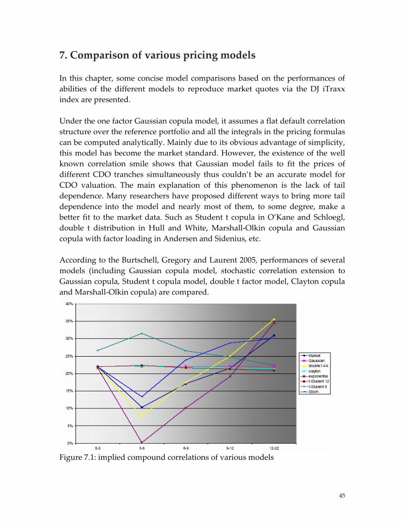
7. Comparison of various pricing models In this chapter, some concise model comparisons based on the performances of abilities of the different models to reproduce market quotes via the DJ iTraxx index are presented. Under the one factor Gaussian copula model, it assumes a flat default correlation structure over the reference portfolio and all the integrals in the pricing formulas can be computed analytically. Mainly due to its obvious advantage of simplicity, this model has become the market standard. However, the existence of the well known correlation smile shows that Gaussian model fails to fit the prices of different CDO tranches simultaneously thus couldn’t be an accurate model for CDO valuation. The main explanation of this phenomenon is the lack of tail dependence. Many researchers have proposed different ways to bring more tail dependence into the model and nearly most of them, to some degree, make a better fit to the market data. Such as Student t copula in O’Kane and Schloegl, double t distribution in Hull and White, Marshall‐Olkin copula and Gaussian copula with factor loading in Andersen and Sidenius, etc. According to the Burtschell, Gregory and Laurent 2005, performances of several models (including Gaussian copula model, stochastic correlation extension to Gaussian copula, Student t copula model, double t factor model, Clayton copula and Marshall‐Olkin copula) are compared.

Figure 7.1: implied compound correlations of various models

45

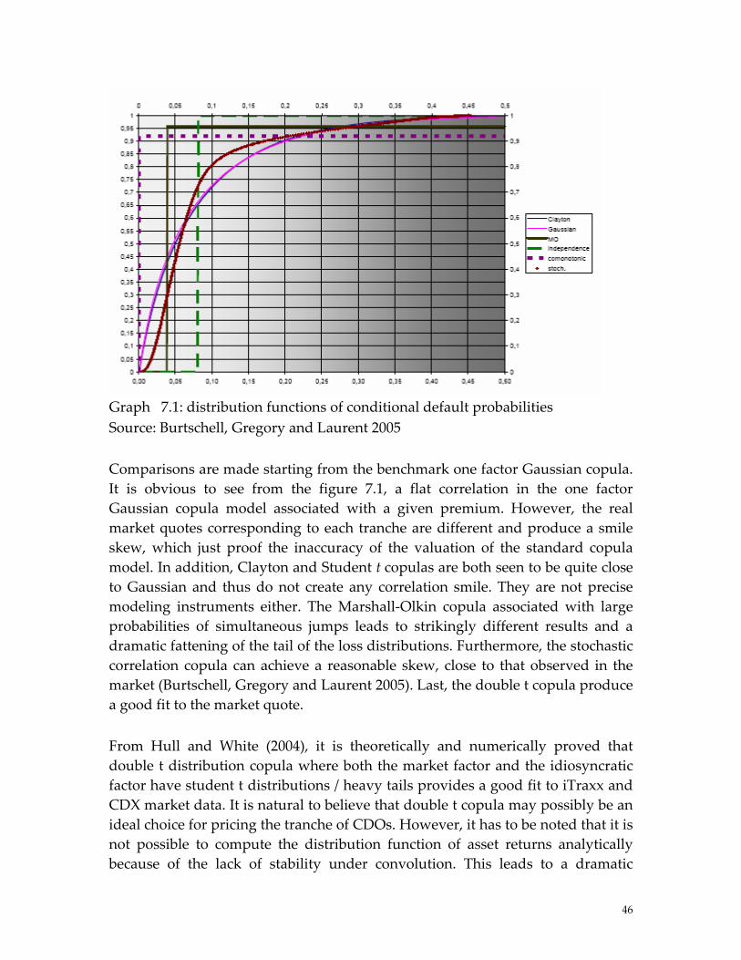
Graph 7.1: distribution functions of conditional default probabilities Source: Burtschell, Gregory and Laurent 2005 Comparisons are made starting from the benchmark one factor Gaussian copula. It is obvious to see from the figure 7.1, a flat correlation in the one factor Gaussian copula model associated with a given premium. However, the real market quotes corresponding to each tranche are different and produce a smile skew, which just proof the inaccuracy of the valuation of the standard copula model. In addition, Clayton and Student t copulas are both seen to be quite close to Gaussian and thus do not create any correlation smile. They are not precise modeling instruments either. The Marshall‐Olkin copula associated with large probabilities of simultaneous jumps leads to strikingly different results and a dramatic fattening of the tail of the loss distributions. Furthermore, the stochastic correlation copula can achieve a reasonable skew, close to that observed in the market (Burtschell, Gregory and Laurent 2005). Last, the double t copula produce a good fit to the market quote. From Hull and White (2004), it is theoretically and numerically proved that double t distribution copula where both the market factor and the idiosyncratic factor have student t distributions / heavy tails provides a good fit to iTraxx and CDX market data. It is natural to believe that double t copula may possibly be an ideal choice for pricing the tranche of CDOs. However, it has to be noted that it is not possible to compute the distribution function of asset returns analytically because of the lack of stability under convolution. This leads to a dramatic

46

increase of computation time and makes it impossible to use this model for some important applications in practice (Kalemanova et al). Considering this problem, Kalemanova et al has introduced the Normal inverse Gaussian (NIG) copula model. The NIG distribution still has higher tail dependence than the Gaussian distribution. In addition, it is stable under convolution under certain conditions. From the Kalemanova et al, The employment of the NIG distribution does not only bring significant improvement with respect to computation times but also more flexibility in the modeling of the dependence structure of a default structure. Copula models with random recovery rate (RR) and random factor loadings (RFL) are introduced by Andersen and Sidenius 2004. They both conform better with the observed phenomena (correlation smile) than standard Gaussian model. For the random recovery rate copula, it is shown to produce a heavy upper tail in portfolio loss distributions, however, its effects on generating a skew in tranche values is small and the RR approach is unlikely to become an efficient method. By comparison, factor loading approach did much better in this respect. At reasonable parameter levels, RFL approach is capable of generating correlation skew very similar to the observed data in the market. Implied copula approach is produced by Hull and White. This approach is slightly different from other copula models (like student t, Clayton, RFL etc) in that they directly specify the distribution of the future environments (hazard rate paths) instead of specifying the copula models as other models do. The outcome of this approach is perfectly good since the model can be exactly fitted to the market quotes for the actively traded CDO tranches. In addition, the model is more intuitive than the base correlation model.

47

8. Conclusion This paper gives an overview of the vast areas of credit derivatives and different products in the market, especially the CDO. For reference, I also address the issues about the CDO tranches, loss distribution and large portfolio approximation etc. Basic valuation methodology and the default correlation model framework are discussed in details. In order to obtain the fair premium of CDO, standard market benchmark model‐‐‐Gaussian copula model is introduced. Mainly due to the existence of the correlation smile, however, the Gaussian copula model couldn’t obtain relatively accurate spreads results. Thus various extension models aiming at improving the performances of fitting the market quotes arise. Nowadays, a good many extension models, such as student t copula, double t copula, stochastic Gaussian copula, Clayton, normal inverse Gaussian copula, RFL Gaussian copula, implied copula model etc , are already introduced in the academic area and nearly all of those models provide a better performances than the industry standard one. Hence companies may select and construct their models based on its own specific requirements and situations. According to Burtschell, Gregory and Laurent 2005, we consider the assessment methodology based on the matching of basket default swap spreads and CDO tranches. For the pricing purpose, once correctly calibrated, student t and Clayton copula models provide similar results as the Gaussian copula models. The Marshall‐Olkin copula leads to strikingly different results and a dramatic fattening of the tail of the loss distribution. The double t lies in between and performs well. In addition, it is found out that Copula models with random factor loading (RFL) as well as Normal inverse Gaussian (NIG) copula model can obtain quite similar correlation smile close to market quotes and considered to be two good pricing models. Impressively, the implied copula model has achieved a perfect fit to the real market price and thus becomes a precise model in some situations. However, there are still limitations of those models. For example, for the RFL model, it is argued that the specific parameterizations and model examples used in the paper were rather simplistic, therefore work remains in uncovering parameters and functional forms that best describe the market; for the perfect copula model, it doesn’t involve the dynamic evolution of hazard rates or credit spreads and thus not appropriate for some instruments, like valuing an one‐year option on a five‐year CDO because this depends on hazard rates between years one and five conditional on what we observe happening during the first year. Further researches may be based on improving those problems.

48

Here it should be kept in mind that the market is at its inception period and all modelling work are inevitably based on a quite limited set of observations, which may not fully representative. Moreover, parameters and models will require revision all the time. Therefore, with the development of the economic market more information about dependence on spread level, maturity, correlation skew etc, will be available. Thus in return, more realistic and hedged performances can be achieved, which leads to further extension and more sophisticated models (Andersen, L. and Sidenius, J. (2004)).

49

References Andersen, L. and Sidenius, J. (2004); Extensions to the Gaussian copula: random recovery and random factor loadings. The Journal of Credit Risk, 1(1): 29‐70 Amato, J and J Gyntelberg (2005): “CDS index tranches and the pricing of credit risk correlations”, BIS Quarterly Review, March, pp 73–87 Barndorff‐Nielsen, O.E. (1997). Normal inverse Gaussian distributions and stochastic volatility modelling. Scandinavian Journal of Statistics 24, 1‐13. Barndorff‐Nielsen, O.E. (1978). Hyperbolic distributions and distributions on hyperbolae. Scandinavian Journal of Statistics 5, 151‐157. Bluhm, C., (2003), CDO Modeling: Techniques, Examples and Applications, Working paper, Hypo Vereinsbank Bomfim, A.N. (2005): Understanding Credit Derivatives and Related Instruments London, Elsevier Academic Press Bomfim (2001), “Understanding Credit Derivatives and their Potential to Synthesize Riskless Assets”, FEDS Paper, Federal Reserve Board. Burtschell, X., Gregory, J. and Laurent, J.‐P. (2005). A comparative analysis of CDO pricing models. Working paper ISFA Actuarial School and BNP Parisbas. Christian Bluhm; Ludger Overbeck; Semi‐analytic Approaches to Collateralized Debt Obligation Modelling；Economic Notes, Volume 33, Number 2, July 2004, pp. 233‐255(23) Daul, S., De Giorgi, E., Lindskog, F. & McNeil, A. (2003). The grouped t‐copula with an application to credit risk. RISK, 16, 73–76. Davide Meneguzzo, Walter Vecchiato (2004); Copula sensitivity in collateralized debt obligations and basket default swaps； The Journal of Futures Markets, Vol. 24, No. 1, 37–70 Demarta, S. & A. McNeil, 2004; the t Copula and Related Copulas, working paper, ETH‐Z.

50

Douglas Lucas (2004), Default Correlation: From Definition to Proposed Solutions, working paper, UBS. Duffie, D. and K. Singleton, “Modeling Term Structures of Defaultable Bonds,” Review of Financial Studies, 12 (1999) 687‐720. Gregory, J., & J.‐P. Laurent, 2004, In the Core of Correlation, RISK, October, 87‐91 Guegan, Dominique and Houdain, Julien, 2005, “Collateralized Debt Obligations Pricing and Factor Models: A New Methodology Using Normal Inverse Gaussian Distributions,” www.defaultrisk.com/pp crdrv 93.htm Hager, S., Schöbel R. (2005): A note on the correlation smile. Tübinger Diskussionsbeitrag 297 (2005) Hull, J. and White, A. (2004). Valuation of a CDO and an Nth‐to‐default CDS without Monte Carlo simulation. Working paper, University of Toronto. Hull, J. and White, A.(2005); the Perfect Copula; Rotman School of Management University of Toronto First Draft: June 2005 Third Draft: July 2005 Jonathan Batten, Warren Hogan. A perspective on credit derivatives [J]. International Review of Financial Analysis, 11 (2002)251‐278 Kalemanova, A., Schmid, B. and Werner, R. (2005). The normal inverse Gaussian distribution for synthetic CDO pricing.Working paper, risklab germany. Kiff, J. and Morrow, R.; Credit derivatives; Bank of Canada Review. Ottawa: Autumn 2000. pg. 3, 9 pgs Laurent, J.‐P., & J. Gregory, 2003, Basket Default Swaps, CDOs and Factor Copulas, ISFA Actuarial School, University of Lyon, working paper available on www.defaultrisk.com. Lehman Brothers (2001), “Credit Derivatives Explained – Market, Products and Regulations”, Structured Credit Research Lehnert,N., Altrock, F., Svetlozar T. Rachev, Stefan Trück, Andre Wilch (2005); Implied Correlations in CDO Tranches; http://www.defaultrisk.com

51

Li, D. X. (2000). On default correlation: a copula factor approach. The Journal of Fixed Income March, 43‐54. McGinty, L., Ahluwalia, R., 2004a. Credit Correlation: A Guide. Credit Derivatives Strategy, JP Morgan Merton, R.C., “On the Pricing of Corporate Debt: The Risk Structure of Interest Rates,” Journal of Finance, 29 (1974), 449‐70. Michael B. Walker (2005); a Term‐Structure Model for Collateralized Debt Obligations Michael B. Walker (2006); CDO Models – Towards the Next Generation: Incomplete Markets and Term Structure; www.defaultrisk.com. O’Kane D. & L. Schloegl, 2003, The Large Homogeneous Portfolio Approximation with the Student t Copula, working paper, Lehman Brothers. Vasicek, O. (1987). Limiting loan loss probability distribution. Technical Report, KMV Corporation Van der Voort, M., 2005, “Factor copulas: totally external defaults,” ABN Amro and Erasmus University of Rotterdam, Working Paper

52