Collateral, Risk Management, and theDistribution of Debt Capacity

ADRIANO A. RAMPINI and S. VISWANATHAN∗

Journal of Finance 65 (2010) forthcoming

ABSTRACT

Collateral constraints imply that financing and risk management are fundamentallylinked. The opportunity cost of engaging in risk management and conserving debtcapacity to hedge future financing needs is forgone current investment, and is higherfor more productive and less well-capitalized firms. More constrained firms engagein less risk management and may exhaust their debt capacity and abstain from riskmanagement, consistent with empirical evidence and in contrast to received theory.When cash flows are low, such firms may be unable to seize investment opportunitiesand be forced to downsize. Consequently, capital may be less productively deployedin downturns.

Financing and risk management are fundamentally linked as both involve promises to

pay that are limited by collateral constraints. Engaging in risk management and conserving

debt capacity have an opportunity cost – current investment is forgone. This cost is higher for

more constrained firms. This insight has important implications for the extent of corporate

risk management.

∗Duke University. We thank Michael Fishman, Denis Gromb, Jeremy Stein, and the acting editor,two referees, as well as Amil Dasgupta, Douglas Diamond, Emmanuel Farhi, Alexander Gumbel, YaronLeitner, Christine Parlour, Guillaume Plantin, David Scharfstein, David Skeie, Rene Stulz, and seminarparticipants at the Federal Reserve Bank of New York, Southern Methodist, Duke, Michigan State, INSEAD,Vienna, Stockholm School of Economics, Mannheim, Illinois, Zurich, British Columbia, Toronto, Minnesota,ETH Zurich, Ohio State, Columbia, Maryland, Washington University in St. Louis/the Federal ReserveBank of St. Louis, Collegio Carlo Alberto, the European University Institute, the Jackson Hole FinanceGroup, the University of Chicago GSB conference “Beyond Liquidity: Modeling Frictions in Finance andMacroeconomics,” the 2008 Basel Committee/CEPR/JFI conference, the Paul Woolley Centre conferenceat LSE, the 2008 North American Summer Meeting of the Econometric Society, the 2008 SED Meeting,the 2008 NBER Summer Institute in Capital Markets and the Economy, the 2008 Minnesota Workshopin Macroeconomic Theory, the 2008 Washington University Conference on Corporate Finance, the 2008Conference of Swiss Economists Abroad, the 2009 AEA Meeting, the European Winter Finance Conference,and the 2009 FIRS Conference for helpful comments and Wei Wei for research assistance. This paper waspreviously circulated under the title “Collateral, Financial Intermediation, and the Distribution of DebtCapacity.”

1

We provide a dynamic model of collateralized firm financing in which firms have access

to complete markets, subject to collateral constraints due to limited enforcement, and hence

are able to engage in risk management. Firms may choose to conserve debt capacity to

take advantage of future investment opportunities. Our model predicts that firms with less

internal funds exhaust their debt capacity rather than conserve it, rendering them unable to

seize investment opportunities. In contrast, firms with more internal funds conserve some of

their debt capacity, allowing them to seize investment opportunities. Moreover, our model

implies that the more constrained firms hedge less and may not engage in risk management at

all, because the financing needs for investment override hedging concerns. Thus, there is an

important connection between firm financing and risk management: both involve promises

to pay by the firm that are limited by collateral. The prediction of our model for corporate

risk management is consistent with the evidence that smaller firms, which are likely to be

more financially constrained, hedge less. This fact is considered a puzzle in the literature,

since models that take up-front investment as given predict that financially constrained firms

are effectively risk averse and should hedge (see, for example, Froot, Scharfstein, and Stein

(1993)). In contrast, our model suggests that the absence of risk management by severely

constrained firms should not be considered a puzzle.

The main intuition is that both conserving debt capacity and conserving net worth in a

state-contingent way – by engaging in risk management or arranging for loan commitments

– have an opportunity cost as they reduce the amount of net worth available for current

investment. The opportunity cost of forgone investment is high for firms with few internal

funds, because they operate at a smaller scale and hence are more productive at the margin.

Similarly, when firms differ in their productivity, the opportunity cost is higher for the more

productive firms and thus such firms are more likely to exhaust their debt capacity and

abstain from risk management.

This observation has important implications for the distribution of debt capacity, which

is endogenous in our model. Suppose that in downturns cash flows are low but investment

opportunities arise as the price of capital is also low. More productive firms and firms that

are less well capitalized may be unable to take advantage of such investment opportunities.

Indeed, these firms may be forced to scale down investment during downturns because their

debt capacity is exhausted. Note that this is constrained efficient since firms optimally

choose to exhaust their debt capacity and abstain from hedging in our model, and is not

due to firms’ lack of ability to hedge. In contrast, less productive and more well-capitalized

firms are able to use their free debt capacity in such times to expand. The dynamics of

the distribution of debt capacity may imply that capital is less productively deployed in

2

downturns and thus that distributional effects amplify aggregate productivity shocks.

Our model allows us to consider the effect of an increase in firms’ ability to collateralize

claims. Such an increase raises firms’ ability to borrow ex ante and hence allows higher

leverage, but increased leverage reduces firms’ net worth ex post. Firms that exhaust their

debt capacity may then be forced to scale down investment even more due to their lower net

worth ex post, that is, the contraction of such firms may be more severe. Thus, higher collat-

eralizability may render the amount of capital deployed by productive and poorly capitalized

firms more volatile. The effects highlighted in this paper may thus become more pronounced

as financial innovation increases firms’ ability to collateralize claims, as has arguably been

the case recently.

Finally, the minimum down payment requirements, or “lending standards,” in our model

vary endogenously with expected capital appreciation. When the price of capital is expected

to rise, down payment requirements are low because the higher expected collateral value

allows increased borrowing. When the price of capital is expected to decline, firms are

forced to deleverage. This prediction is empirically plausible and consistent with anecdotal

evidence.

The collateral constraints in our model are derived from an explicit dynamic model with

limited enforcement, which is the only friction in the model. Our assumptions on limited

enforcement imply that firms have access to complete markets in one-period-ahead state-

contingent claims subject to state-by-state collateral constraints, that is, they can issue

promises to pay against each state up to a fraction of the collateral value in that state.

Importantly this allows firms in our model to engage in risk management. Thus, in contrast

to most of the literature, we do not assume that aggregate states are not contractible. Our

collateral constraints are similar to the ones in Kiyotaki and Moore (1997), except that

they are state contingent, and are derived in an economy with limited contract enforcement

in the spirit of Kehoe and Levine (1993, 2001, 2008). We assume that firms have limited

commitment and can default on their promises to pay and abscond with all cash flows

and a fraction of capital. We further assume that firms that default cannot be excluded

from the market for capital or from borrowing and lending. Kehoe and Levine (1993) and

most of the subsequent literature assume instead that borrowers who default are excluded

from intertemporal trade.1 Deriving collateral constraints from a dynamic environment with

limited commitment, as we do, allows for explicit analysis of their dynamic effects without

requiring “ad hoc” extensions of constraints motivated by a static contracting problem to

1A notable exception is Lustig (2007), who considers limited enforcement similar to that in our model inan endowment economy.

3

a dynamic setting. Indeed, we think our model provides a useful framework for addressing

many questions in dynamic corporate finance.

The paper proceeds as follows: Section I provides the model of collateral constraints

due to limited enforcement, defines debt capacity and financial slack, and discusses the

implementation with loan commitments. Section II studies how firms’ decisions to conserve

or exhaust debt capacity vary with their productivity and considers the implications for the

distribution of debt capacity in the cross-section. Section III considers the effect of firm net

worth on firms’ decisions to exhaust debt capacity and the implications for risk management,

and contrasts our conclusions with those of received theory. Section IV discusses the related

literature. Section V concludes. All proofs are in the Appendix.

I. A Dynamic Model of Collateralized Financing

We propose a dynamic model of collateralized financing. We consider an economy in

which limited enforcement constrains firms’ ability to make credible promises. We show that

this economy is equivalent to an economy in which lending is subject to collateral constraints.

We define debt capacity, financial slack, and risk management explicitly and show how to

interpret loan commitments in the context of the model.

A. Environment

Consider a finite horizon T , with dates t = 0, 1, . . . , T.2 Let there be a continuum of agents

(of measure one) that are risk neutral, subject to limited liability, and have preferences over

(nonnegative) dividends given by

E

[T∑

t=0

βtdt

], (1)

where β ≤ 1 is the rate of time preference. There are two goods in the economy, consumption

goods and capital. Each agent is endowed with w0 units of the consumption good at time 0

and no capital. Agents also have access to a production technology described below. These

agents can be interpreted as entrepreneurs or firms that have a financing need, and we refer

to them throughout as firms.

Denote the state at date t by st ≡ {s0, s1 . . . , st}, which includes the history of realizations

of the stochastic process sτ for dates τ = 0, 1, . . . , t, and the set of states at date t by S t.3

2From Section II onwards, we set T = 2 for simplicity. Rampini and Viswanathan (2010) analyze astationary model with an infinite horizon and a constant price of capital.

3Let S0 = s0, that is, a singleton.

4

Denote the probability of state st by π(st) and the probability of state st+1 given state st by

π(st+1|st). Similarly, denote the set of states st+1 given st by S t+1|st.

The firms have access to a standard neoclassical production technology. An amount of

capital k(st) invested at time t in state st ∈ S t returns, at time t+1 in state st+1 ∈ S t+1|st, a

cash flow A(st+1)ft(k(st)) in consumption goods as well as the capital k(st).4 The production

function ft(·) is strictly increasing and (weakly) concave, and productivity is strictly positive

in all states, that is, A(st+1) > 0, ∀st+1 ∈ S t+1, t = 0, 1, . . . , T − 1.

We assume that firms vary either in terms of their productivity or net worth. In Section II

we assume that the production function has constant returns to scale and that firms differ

in the productivity A(st+1) of their technology, and we analyze how the decision to conserve

debt capacity depends on productivity. In Section III we assume decreasing returns instead

and study the connection between net worth and risk management when firms differ in

their time 0 net worth w0. Thus, agents in our model are of different types, although the

dependence (of productivity or net worth) on type is suppressed throughout.

In addition to the firms described above, there is also a continuum of lenders (of measure

one) in the economy that are unconstrained and risk neutral and that discount the future at

rate β ≤ 1, which equals the agents’ rate of time preference. Lenders have a large endowment

of funds in all dates and states. Lenders cannot run the production technology. Lenders have

a large amount of collateral and hence are not subject to enforcement problems but rather

are able to commit to deliver on their promises. Lenders are thus willing to provide any

state-contingent claim at an expected rate of return R = 1/β subject to firms’ enforcement

constraints.5

We assume that markets are complete but there is limited enforcement; firms can abscond

with the cash flows from the production technology and with fraction 1 − θ of capital.

Importantly, we assume that firms cannot be excluded from future borrowing or the market

for capital. Below we show that this is equivalent to assuming the following specification of

financing constraints: firms can borrow in a state-contingent way at time t up to θ ∈ (0, 1)

times the resale value of capital against each state at time t + 1.6

Finally, we assume that consumption goods can be transformed into capital (and vice

4We assume that capital does not depreciate for simplicity, but standard neoclassical depreciation at rateδ ∈ (0, 1) could be easily accommodated.

5The focus of our paper is thus on the implications of collateral constraints of firms and not lenders.6Considering capital explicitly and separately from consumption goods is important for two reasons. First,

this is the standard assumption and notation in the theory of investment and macroeconomics. Second, thismakes the role of collateral in financing explicit, which is central to our analysis and delivers a model thatis empirically plausible in our view.

5

versa) at a cost q(st) per unit of capital at time t in state st ∈ S t. We refer to q(st) as the

price of capital. The assumption that the price of capital is exogenously determined by a

technological rate of transformation allows us to focus on the corporate finance implications

of our model, whereas much of the literature focuses on the endogenous determination of this

price (see, most notably, Kiyotaki and Moore (1997)).7 Moreover, our assumption effectively

reduces our model to a one-good economy and thus the allocation is constrained efficient.8

B. Limited Enforcement

Suppose that enforcement of contracts is limited as follows: firms can default on their

promises, that is, walk away from their obligations and abscond with all cash flows and the

fraction 1 − θ of capital, and lenders can seize only the fraction θ of the capital and do not

have access to any other enforcement mechanism. In particular, firms cannot be excluded

from further borrowing or from purchasing capital. Thus, enforcement is limited as in Kehoe

and Levine (1993) but unlike in their model, firms cannot be excluded from intertemporal

markets here.9,10

The firm chooses (nonnegative) dividends {d(st)}, (nonnegative) capital levels {k(st)},and net payments {p(st)}, ∀st ∈ S t, t ∈ {0, 1, . . . , T}, to maximize the expected discounted

value of dividends (1) subject to the budget constraints at time 0 (equation (2)) and at

time t = 1, 2, . . . , T (equation (3)), ∀st ∈ S t,

w(s0) ≥ d(s0) + q(s0)k(s0) + p(s0) (2)

A(st)ft−1(k(st−1)) + q(st)k(st−1) ≥ d(st) + q(st)k(st) + p(st), (3)

the lender’s participation constraint at time 0,

E

[T∑

t=0

R−tpt

∣∣∣∣∣ s0

]≥ 0, (4)

and the enforcement constraints at time τ , ∀τ > 0, τ ≤ T, ∀sτ ∈ Sτ ,

E

[T∑

t=τ

βt−τdt

∣∣∣∣∣ sτ

]≥ E

[T∑

t=τ

βt−τ dt

∣∣∣∣∣ sτ

], (5)

7Endogenizing the price would not change our main conclusions, however.8More specifically, we can show that any distribution of the initial net worth leads to a competitive

equilibrium that is constrained efficient, that is, no other allocation can Pareto dominate the competitiveallocation and satisfy the collateral constraints.

9If θ were equal to zero, that is, if the firm could abscond with all cash flows and all capital and wouldnot be excluded from future lending, firms could not borrow at all (see Bulow and Rogoff (1989)).

10In practice, such exclusion is in fact rather limited. Moreover, this assumption implies a tractabledynamic model of collateral constraints with empirically plausible implications.

6

for all {d(st)}t≥τ that the firm could achieve after absconding, that is, for all continuation

policies {d(st), k(st), p(st)}t≥τ that solve the above problem from time τ onward given net

worth w(sτ) ≡ A(sτ)fτ−1(k(sτ−1)) + q(sτ)k(sτ−1)(1 − θ).

The enforcement constraints (5) require that, when the firm keeps its promises, it attains

a value that is at least as high as the value attained by absconding. The firm’s problem

after absconding at time τ in state sτ is identical to the continuation problem at time τ in

state sτ , when it does not default, except that the firm has net worth A(sτ)fτ−1(k(sτ−1)) +

q(sτ)k(sτ−1)(1−θ) after default, as opposed to net worth A(sτ )fτ−1(k(sτ−1))+q(sτ)k(sτ−1)−p(sτ ) when it does not default.

C. Collateral Constraints Due to Limited Enforcement

We show that the model with limited enforcement is equivalent to a model with state-

contingent one-period debt subject to state-contingent collateral constraints. Thus, our

model implies intuitive collateral constraints that facilitate the analysis of optimal dynamic

collateralized financing.

The equivalence obtains in two steps. First, the enforcement constraints imply that the

firm can only credibly promise payment streams with present value less than or equal to

the value of capital the firm cannot abscond with.11 Second, any long-term contract that

satisfies this restriction can be implemented with a sequence of one-period debt contracts.

Hence, long-term contracts are irrelevant.12

Proposition 1: Enforcement constraints (5) are equivalent to collateral constraints

q(st)θk(st−1) ≥ Rb(st), (6)

where b(st) is one-period-ahead state-contingent debt with

b(st) = E

[T∑

τ=t

R−(τ−(t−1))pτ

∣∣∣∣∣ st

], ∀st ∈ S t, t = 1, 2, . . . , T.

Proposition 1 shows that, given our assumptions about the limits on enforcement, the

constraints can equivalently be formulated as collateral constraints in the spirit of Kiyotaki

11Firms’ ability to deploy capital productively results in higher cash flows, but firms are unable to pledgethese cash flows since they can abscond with them, and hence firms’ productivity does not affect the collateralconstraints directly.

12In contrast, when firms can be excluded from intertemporal trade, long-term contracts are not generallyirrelevant.

7

and Moore (1997) but importantly are state contingent.13 Given Proposition 1 we can restate

the firm’s problem restricting attention to one-period-ahead state-contingent debt without

loss of generality by restating equations (2) and (3) as

w(s0) + E[b1|s0

]≥ d(s0) + q(s0)k(s0) (7)

A(st)ft−1(k(st−1)) + q(st)k(st−1) + E[bt+1|st

]≥ d(st) + q(st)k(st) + Rb(st), (8)

and by replacing the enforcement constraints (5) with the collateral constraints (6).14 The

firm chooses (nonnegative) dividends {d(st)}, (nonnegative) capital levels {k(st)}, and one-

period-ahead state-contingent debt {b(st)}, ∀st ∈ S t, t = 0, 1, . . . , T, to maximize (1) subject

to (6) to (8). We study this problem henceforth.15

Note that if the firm promises to pay Rb(st+1) in state st+1 at time t + 1, it receives an

amount of funds π(st+1|st)b(st+1) at time t. This guarantees the lender an expected return

of R on the loan. Moreover, the amount that the firm can credibly promise to repay at

time t + 1 in state st+1 is limited to a fraction θ of the resale value of capital in that state.

The firm receives a total amount of funds E[bt+1|st] at time t for all promises to pay issued

against states st+1 ∈ S t+1|st.

The equivalent formulation has the important advantage that the implementation of the

optimal dynamic contract is rather simple: firms have access to state-contingent secured

loans only. Such lending arrangements are thus decentralized relatively easily by defining an

equilibrium with collateral constraints with trade in state-contingent one-period loans that

are subject to a state-contingent collateral constraint equal to the fraction θ times the resale

value of capital.16 Thus, firms in our model have exogenous net worth w0 at time 0 and meet

all subsequent financing needs with internal funds or secured debt.17

13Lustig (2007) considers a similar outside option in an endowment economy and Lorenzoni and Walentin(2007) consider collateral constraints with a similar motivation in an economy with constant returns to scale.The original formulation of the enforcement constraints is in the same spirit as the one used to endogenizedebt constraints in Kehoe and Levine (1993), although the limits on enforcement are different here. Kehoeand Levine assume that borrowers who default are excluded from intertemporal markets whereas we assumethat firms cannot be excluded.

14Note that we set E[bT+1|sT ] = 0 and clearly k(sT ) = 0.15Another advantage of this equivalent formulation is that the constraint set (6), (7), and (8) is convex.16Similarly, Alvarez and Jermann (2000) define an equilibrium with solvency constraints to decentralize

optimal allocations in an environment with limited commitment as in Kehoe and Levine (1993). The solvencyconstraints in their model are agent and state specific in contrast to the simple collateral constraints here.

17We interpret this implementation as firms having access to equity financing at time 0 and not subse-quently; that is, initial net worth is determined in an initial public offering and there are no seasoned equityofferings, which we find empirically plausible.

8

D. Debt Capacity, Financial Slack, and Risk Management

Our model allows us to provide a precise definition of debt capacity and financial slack.

Given an amount of capital k(st), the firm has debt capacity q(st+1)θk(st) for state st+1 at

time t + 1 and can issue promises Rb(st+1) up to that amount. By promising less than its

debt capacity, the firm can keep financial slack h(st+1), where

h(st+1) ≡ q(st+1)θk(st) − Rb(st+1)

for state st+1 at time t + 1. Note that using this definition we can write the collateral

constraints (6) simply as nonnegative financial slack constraints, that is,

h(st) ≥ 0, ∀st ∈ S t, t ∈ {1, 2, . . . , T}.

The firm’s net worth in state st+1 at time t + 1 can now be written in two equivalent ways

as

w(st+1) = A(st+1)ft(k(st)) + q(st+1)k(st) − Rb(st+1)

= A(st+1)ft(k(st)) + q(st+1)k(st)(1 − θ) + h(st+1).

The firm can conserve net worth in a state-contingent way by not exhausting debt capacity

(as the former expression above suggests) or, in other words, by keeping financial slack (as

the latter expression suggests). Similarly, not keeping any financial slack is equivalent to

exhausting the debt capacity.

Define the minimum down payment ℘(st) at time t in state st as the minimum amount

that a firm needs to pay down per unit of the asset, which is the price of the asset minus

the collateralizable fraction of the discounted expected resale value, that is, the price of the

asset minus the maximum amount that the firm can borrow against the asset,

℘(st) ≡ q(st) − R−1E[qt+1|st

]θ.

The firm’s problem can now be written recursively for each state st at time t assuming

that the firm always makes the minimum down payment but may keep nonnegative state-

contingent financial slack, that is, may engage in risk management by purchasing one-period

Arrow securities subject to short sale constraints, as

Vt(w(st), st) = max{d(st),k(st),w(st+1),h(st+1)}

d(st) + βE[Vt+1(wt+1, s

t+1)|st]

9

subject to

w(st) ≥ d(st) + ℘(st)k(st) + R−1E[ht+1|st

],

A(st+1)ft(k(st)) + q(st+1)k(st)(1 − θ) + h(st+1) ≥ w(st+1),

h(st+1) ≥ 0,

and d(st), k(st), w(st+1) ≥ 0, for all st and st+1 ∈ S t+1|st, t = 0, . . . , T, where the firm’s net

worth is defined as w(st) ≡ A(st)ft−1(k(st−1)) + q(st)k(st−1)(1 − θ) + h(st) and we define

VT+1(·) ≡ 0. The first constraint above makes the trade-off between using net worth for

investment and keeping financial slack by purchasing Arrow securities transparent.

Since borrowing against a particular state reduces the firm’s net worth in that state,

which in turn constrains investment going forward, the firm has a debt overhang problem

in the spirit of Myers (1977). However, in our model the firm can optimally choose its debt

overhang for each state and we analyze how the firm’s choice of its optimal debt overhang

for each state depends on the firm’s productivity and net worth at time t.

Finally, a firm’s capital k(st) and hence its debt capacity are of course not exogenous.

Rather, the firm chooses its capital k(st) endogenously, and thus investment, financing, and

risk management are all jointly endogenously determined.

This model of collateralized borrowing has the property that the minimum down pay-

ment is lower when the price of capital is expected to rise. This property seems empiri-

cally plausible and is consistent with anecdotal evidence that down payment requirements

(or “lending standards”) vary inversely with expected capital appreciation. The minimum

down payment as a fraction of the price of capital at time t in state st, for example, is

℘(st)/q(st) = 1 − R−1E [qt+1|st]/q(st)θ and thus is decreasing in the expected capital ap-

preciation E [qt+1|st] /q(st). Thus, expectations about future asset prices have an important

effect on current down payment requirements. We are not aware of other models that predict

such variation in down payment requirements.

E. Implementation with Loan Commitments

In our model, firms have access to one-period state-contingent loans or, equivalently,

complete markets in one-period Arrow securities, subject to collateral constraints. We now

show how to implement the optimal contract, one-period-ahead state-contingent debt, with

loan commitments. Loan commitments are one way firms can conserve debt capacity and

keep financial slack in a state-contingent way, which is important in practice.

Define a loan commitment as a binding agreement to provide a loan of a particular size

in state st+1 at time t + 1 for a fee paid up front. Clearly, a loan that has zero net present

10

value to the lender when extended at time t+1 requires neither ex ante commitment by the

lender nor up-front fees. Indeed, so far we assume that all loans are of this type, which is

without loss of generality given Proposition 1.

Now consider a loan commitment {c(st), l(st+1), b(st+2)} in which for an up-front fee c(st)

to be paid in state st at time t, the lender agrees to provide a loan l(st+1) > E[b(st+2)|st+1]

in state st+1 at time t + 1 such that

c(st) + π(st+1|st)R−1{−l(st+1) + R−1E[Rb(st+2)|st+1]} = 0,

which means that the loan commitment has zero net present value at time t due to competi-

tion in the market for loan commitments. In contrast, the net present value to the lender of a

loan commitment in state st+1 at time t+1 is NPV (st+1) = −l(st+1)+R−1E[Rb(st+2)|st+1] <

0, that is, negative, which is why it does in fact require a commitment. By taking out such

a loan commitment, the firm effectively increases its net worth in state st+1 at time t + 1 by

NPV (st+1). However, this comes at an up-front cost of c(st) = −π(st+1|st)R−1NPV (st+1)

in terms of fees. But then the firm could equivalently buy state st+1 Arrow securities in the

amount of c(st), which would increase its net worth in state st+1 at time t + 1 by the same

amount.

The key insight is that lining up loan commitments requires internal funds up front and

thus has a cost in terms of reduced investment up front. Arranging for loan commitments

or contingent financing is akin to conserving contingent net worth. Firms that choose to

exhaust their debt capacity thus do not arrange for loan commitments either.

II. The Distribution of Debt Capacity

In this section we study the distribution of debt capacity and the dynamics of investment

by different firms. We also analyze the effect of collateralizability and asset prices on the

extent to which constrained firms might downsize, that is, scale down their investment. We

show that more productive firms may exhaust their debt capacity since the opportunity

cost of conserving debt capacity, which is forgone investment earlier on, is higher for them.

This implies that in states where asset prices and cash flows are low, capital may be less

productively deployed on average, since more productive firms, which have exhausted their

debt capacity, downsize relative to less productive firms.

To simplify, we henceforth assume that T = 2 and that uncertainty is resolved at time 1.

We simplify the notation by dropping the superscript and writing s ∈ S. We also write

time 0 variables as q0 ≡ q(s0) and time t variables as qt(s) ≡ q(st), and employ analogous

11

simplifications for the other variables as well.18

One special case that is of particular interest is the case in which capital is relatively

cheap when cash flows are low, that is, for all s, s+ ∈ S, and s+ > s, q1(s+) > q1(s) but

A1(s+) > A1(s). This is meant to capture the idea that states with lower s are states in

which there is an economy-wide downturn. The downturn implies low cash flows. But in a

downturn capital is relatively cheap, which implies that this may be a good time to invest.

Thus, this is an important scenario in which cash flows and investment opportunities are

negatively correlated. The model allows us to study which firms are likely to be able to

take advantage of such opportunities and which firms are likely to be constrained during

these times. While this case of negative correlation between cash flows and investment

opportunities is especially interesting because of its association with economic downturns or

crises, the main conclusions of our model hold generally. We study the general case below

and make no specific assumptions about the correlation between the price of capital and

productivity, except where explicitly stated.

A. Conserve or Exhaust Debt Capacity?

Consider how a firm’s decision to conserve or exhaust its debt capacity depends on the

firm’s productivity. In order to abstract from net worth effects for now, we assume that

investment exhibits constant returns to scale, that is, ft(kt) = kt and hence f ′t(kt) = 1.

Define the return on the firm’s internal funds when it invests by making the minimum down

payment (that is, by choosing maximal leverage) R1(k0, s) as

R1(k0, s) ≡A1(s)f

′0(k0) + q1(s)(1 − θ)

℘0(9)

and define R2(k1(s), s) analogously. With constant returns to scale, R1(k0, s) does not depend

on k0 and hence we simplify the notation to R1(s) (similarly, we write R2(s) instead of

R2(k1(s), s)). Moreover, we assume that investment at time 1 is sufficiently productive, that

is,

Assumption 1: R2(s) > R, ∀s ∈ S.

This simplifies the analysis by implying that firms are constrained at time 1 and do not

pay dividends before time 2.

Our first main result is that, depending on how productive investment is at time 0, firms

either invest as much as they can and exhaust their debt capacity against all states at time 1

18We drop the conditioning of the expectation operator and write E[·] instead of E[·|s0] henceforth.

12

or stay on the sidelines at time 0 and conserve all their net worth and debt capacity for

state s′ at time 1, at which point they invest the maximal amount. The state s′ is the state

in which the return is the highest, that is, s′ ∈ arg maxs∈S R2(s).19

Proposition 2: Under Assumption 1 and with constant returns to scale, productive firms

invest at time 0 and exhaust their debt capacity, that is, if

E [R1R2] > maxs

{RR2(s)},

then k0 = w0/℘0. Less productive firms stay on the sidelines and conserve their net worth to

invest in the most productive state s′ at time 1, that is, if the condition is not met, k0 = 0,

w1(s′) = R/π(s′)w0, where s′ ∈ arg maxs{R2(s)}.

The condition for investment is E [R1R2] > maxs{RR2(s)} and thus firms with higher

productivity in the first period, say higher E [R1], are more likely to invest and exhaust their

debt capacity, all else equal. Moreover, the correlation between returns in the first period

and returns in the second period, that is, investment opportunities, of course also matters.

Higher autocorrelation of returns makes investment more likely. Hence, firms are more likely

to exhaust their debt capacity when returns are more persistent.

B. Downsizing of Productive Firms

Now consider a firm that invests at time 0 and exhausts its debt capacity. Such a firm

may not be able to deploy as much capital at time 1 as it deploys at time 0, and thus it

may be “forced to” downsize. This occurs in a state s in which cash flows A1(s)f0(k0) are

sufficiently low and, importantly, occurs despite the fact that the firm could arrange for

contingent financing. The firm chooses not to do so, however, because the opportunity cost

is too high.

Proposition 3: Firms that exhaust their debt capacity are “forced to” downsize at time 1

in state s, that is, k1(s) < k0, if A1(s) is sufficiently low.

Proposition 3 implies that productive firms may downsize when less productive firms,

which did not previously invest, expand. To understand this result consider the simplest

case in which firms differ in expected productivity at time 0 only. In that case, the more

productive firms invest at time 0 and contract at time 1 in states in which cash flows are

low, while the less productive firms stay on the sidelines and expand at time 1. When firms’

19Given the assumption of constant returns to scale, the bang-bang nature of the solution is expected.

13

productivity exhibits positive persistence, as is arguably the case, then average productivity

may decline in the low cash flow states.

C. Effect of Collateralizability on Contraction

A key parameter of the collateral constraint is collateralizability θ. This parameter

depends on the nature of capital considered. For example, it likely differs depending on the

tangibility of capital, that is, on whether capital is physical capital or intangible capital,

as well as on the type of tangible capital, for example, on whether capital is structures or

equipment. Moreover, the efficiency of the legal enforcement should affect collateralizability.

Hence, financial innovation that increases enforceability should increase the collateralizability

of capital.

When collateralizability θ increases, firms that invest at time 0 may downsize to a greater

extent. Thus, factors such as financial innovation that increase collateralizability may result

in more severe contractions of firms that exhaust their debt capacity. This means that the

effects we stress in this paper may become even more important over time as the ability to

collateralize increases, consistent with recent events in financial markets.

Proposition 4: With higher collateralizability, firms that exhaust their debt capacity may

be forced to downsize to a greater extent. Suppose the parameters are as in Proposition 3

such that k1(s)/k0 < 1. Then ∂∂θ

(k1(s)/k0) < 0 as long as q1(s)/q2(s) > k1(s)/(Rk0).

This condition is satisfied, for example, when q1(s) = q2(s). A higher θ has two effects.

First, the firm is able to pledge more funds at time 0 and hence has less net worth left at

time 1. Second, the firm has greater ability to borrow at time 1 going forward and hence

requires a smaller down payment in terms of net worth then. The two effects go in opposite

directions, but as long as the price of capital is not too much higher at time 2, the first effect

dominates: higher leverage due to higher pledgeability leads to a more severe contraction in

capital.

D. Effect of Asset Prices on Contraction

The price of capital q1(s) at time 1 affects the extent of the contraction since it affects

firms’ net worth as well as the down payment required to purchase capital:

Proposition 5: Firms that exhaust their debt capacity downsize to a greater extent when

asset prices fall by a lesser amount, that is, ∂∂q1(s)

(k1(s)/k0) < 0.

Note that by Assumption 1 firms invest all their net worth at time 1, that is, as much as

14

possible, so any contraction in investment is due to changes in firms’ net worth or the down

payment requirement. A higher price of capital at time 1 in state s has two effects, namely,

it raises net worth, since firms retain fraction 1 − θ of the resale value of capital, while at

the same time it raises the down payment requirement ℘1(s). The second effect dominates

the first. The higher the price of capital, the more capital needs to be reduced as more net

worth is required to purchase capital. Thus, a lower price of capital allows firms to deploy

more capital.20

III. Net Worth and Risk Management

This section considers the effect of firm net worth and the implications of our model for

risk management. The model shows that there is an important connection between firm

financing and risk management. In particular, we show that more financially constrained

firms optimally choose less risk management, consistent with the data and in contrast to

the extant results in the literature. The most constrained firms in our model choose not to

hedge at all, as the financing needs for investment override the hedging concerns.

A. Role of Firm Net Worth

Firms’ net worth plays no role in the analysis of Section II due to the assumption of

constant returns to scale. To study the effect of firm net worth, we drop this assumption

and instead assume decreasing returns to scale.

Assumption 2: ft(kt) is strictly increasing, strictly concave, and satisfies limkt→0 f ′t(kt) =

∞ and limkt→∞ f ′t(kt) = 0.

To make the point as simply as possible, suppose there are strictly decreasing returns

at time 0 only, and that the technology has constant returns to scale at time 1 as before.

The firm chooses k0 > 0 at time 0 and hence has positive net worth in all states at time 1.

Moreover, under Assumption 1, the firm invests all its net worth at time 1 in all states,

which implies k1(s) > 0. If the firm hedges, it conserves net worth for the most productive

state at time 1 only. However, the extent to which firms engage in risk management depends

on their net worth. Indeed, the firms do not hedge at all if their net worth is below some

threshold.

20In Proposition 5 we keep the price of capital at time 2 fixed. But the same result obtains if we insteadassume that the price of capital at time 2 equals the price of capital at time 1, that is, q1(s) = q2(s), ∀s ∈ S.

15

Proposition 6: Under Assumption 1 and Assumption 2 at time 0 only, firms with net

worth below w0 exhaust their debt capacity and do not engage in risk management, while

firms with net worth exceeding the threshold conserve some net worth for the state with the

highest productivity at time 1, that is, for state s′ ∈ arg maxs{R2(s)}.

This result is closely related to the result in Proposition 2 that productive firms exhaust

their debt capacity. With decreasing returns, firms with low net worth operate at lower

scale and hence are more productive at the margin, leading them to exhaust their debt

capacity. Firms that are sufficiently well capitalized conserve additional net worth for the

most productive state at time 1 and keep their time 0 investment unchanged. Thus, firms

are hedging investment opportunities.21

We now show that this result obtains generally with decreasing returns to scale in both

periods.22 Firms optimally exhaust their debt capacity against all states and hence abstain

from risk management if their net worth is sufficiently low.

Proposition 7: Under Assumption 2 at time 0 and 1, firms with sufficiently low net worth

do not engage in risk management.

Intuitively, for very low net worth, the return on investing the firm’s net worth R1(k0, s)

becomes so high that it must eventually exceed the return on conserving debt capacity R/π(s)

for all states. For very low net worth the primary concern must be financing investment, not

risk management. In other words, collateral constraints limit the extent to which funds can

be shifted both over time as well as across states. If funds are sufficiently scarce at time 0, it

is optimal to shift as many funds as possible to time 0, rendering firms unable to shift funds

across states at time 1, that is, unable to hedge.

Firms that are sufficiently well capitalized, on the other hand, engage in complete risk

management at time 0, that is, hedge to the point where the marginal value of net worth is

equalized across all states at time 1.

Proposition 8: Suppose that Assumption 2 holds at time 0 and 1 and that A2(s) is suffi-

ciently high, ∀s ∈ S, such that the firm is constrained in all states at time 1. (i) Capital levels

k0 and k1(s), ∀s ∈ S, are increasing in net worth w0, and strictly increasing as long as at

least one collateral constraint binds at time 0, and k0 is constant otherwise. (ii) There exists

a threshold level of net worth w0 such that all firms with net worth exceeding the threshold

engage in complete risk management at time 0, that is, the marginal value of net worth is

21Firms hedge states in which the marginal value of net worth is high either due to investment opportu-nities, as here, or due to low cash flows when returns to scale are decreasing, as below.

22Note that Proposition 7 does not require that the firm is constrained in the second period.

16

equalized across all states at time 1.

When firms’ net worth w0 is very low, the return on investing at time 0 is so high that it

exceeds the return on hedging for all states. As net worth and hence investment increases, the

return on investing at time 0 falls and firms hedge progressively more states until threshold

w0 is reached, at which point firms hedge all states.

To illustrate Propositions 7 and 8, we compute a numerical example. For simplicity,

we assume that there are five equally probable states at time 1, that the price of capital is

constant in all dates and states, and that the level of productivity at time 2 is constant across

states. Thus, the only reason that investment at time 1 varies across states in this example

is because firms may optimally not engage in complete risk management. The parameters

of the example and results are reported in Figures 1 and 2.

The first-order conditions imply the following equation determining the economic trade-

off, ∀s ∈ S,

E [R1(k0)R2(k1)] ≥ RR2(k1(s), s), (10)

where the left-hand side is the expected return on investment at time 0 (and reinvestment

at time 1) and the right-hand side is the expected return on conserving net worth for state s

and investing then. Panel A of Figure 1 shows investment k0 and state-contingent borrowing

b1(s), and Panel B shows financial slack h1(s) as a function of the firm’s net worth w0 at

time 0. Investment is strictly increasing in net worth below a threshold w0 and constant

above the threshold, as Part (i) of Proposition 8 shows. For very low net worth, the left-hand

side of equation (10) strictly exceeds the right-hand side for all states, that is, all collateral

constraints bind and the firm exhausts its debt capacity against all states as Proposition 7

implies. As the firm’s net worth and hence investment increases, equation (10) first holds

with equality for the state with the lowest cash flow at time 1, as this is the state with the

lowest net worth and hence the highest return on internal funds; the firm no longer exhausts

its debt capacity against that state and instead keeps some financial slack for that state.

As the firm’s net worth increases further, equation (10) holds with equality for progressively

more states, and the firm starts to conserve debt capacity for these states as well. Once

net worth reaches the threshold w0, the firm keeps some slack for all states, as Part (ii) of

Proposition 8 implies, at which point E[R1(k0)] = R and time 0 investment is constant. If,

at a given level of wealth, the firm conserves debt capacity for a particular state, then it

conserves debt capacity for all states with lower cash flow than that. Moreover, the firm has

the same net worth at time 1 for all states for which it keeps financial slack. These results

are illustrated in the figure and can be readily seen from equation (10), which holds with

equality for all such states.

17

Panel C of Figure 1 shows investment k1(s) and state-contingent borrowing b2(s) at

time 1. Investment is again increasing in time 0 net worth (as implied by Part (i) of Proposi-

tion 8). Borrowing is now strictly increasing in net worth as, given the parameters, the firm

is constrained in all states at time 1. The firm has the same net worth in all states for which

it keeps financial slack at a given wealth level, and hence investment and borrowing are the

same in all these states (which can be seen from equation (10) as argued above). Figure 2

shows the multipliers on the collateral constraints at time 0 and 1. The time 0 multipliers

are decreasing in time 0 net worth w0 and drop to 0 one by one as the firm starts to conserve

debt capacity for progressively more states at time 1. To see this from equation (10), note

that the multipliers on the collateral constraints at time 0 are proportional to the differ-

ence between the left-hand and right-hand sides. The time 1 multipliers are decreasing and

strictly positive in our example and, for a given net worth, coincide for all states for which

the collateral constraint is slack. The example thus illustrates our main conclusion that more

constrained firms choose less risk management.

B. Reconsidering Risk Management

The state-contingent loans in our model allow firms to engage in “corporate risk man-

agement.” Conserving state s contingent debt capacity amounts to buying state s Arrow

securities, that is, partially hedging the amount of net worth in that state. The main theory

of risk management, formalized by Froot, Scharfstein, and Stein (1993), is based on the

effective risk aversion of firms subject to financial constraints. The rationale for hedging ac-

cording to this theory is that when firms are subject to financial constraints, hedging ensures

that firms have sufficient internal funds to take advantage of investment opportunities. Im-

portantly, this intuition suggests that financially constrained firms should hedge as they are

effectively risk averse. In practice, however, large firms, which are arguably less financially

constrained, hedge while small firms, which are likely more financially constrained, often

do not engage in risk management. This fact thus presents an important puzzle from the

vantage point of received theory. Our theory resolves this risk management puzzle, since it

predicts that the more constrained firms, that is, the more productive or less well-capitalized

firms, exhaust their debt capacity and hence do not hedge. In our model, firms’ ability to

credibly promise to pay is limited, and firms have an incentive to hedge net worth in the low

state for the usual reasons. However, up-front investment is endogenous in our model and the

overriding concern may be to finance up-front investment. Indeed, the more constrained the

firm, the more likely it is that investment financing needs override hedging concerns. This is

the main implication of our model for risk management. Thus, we expect that smaller firms,

18

which are likely more financially constrained, hedge less and as a result are more sensitive to

aggregate fluctuations than larger firms, consistent with empirical evidence.23 In contrast,

Froot, Scharfstein, and Stein (1993) take up-front investment as exogenously given in their

model, in effect making risk management the only concern, and thus reach the opposite

conclusion.

Our results can be reconciled with the received theory by noting that we provide a

dynamic theory of risk management. Received theory is essentially static and argues that

firms hedge to shift funds to the states that have the highest marginal value of net worth.

In our dynamic theory of risk management, firms shift funds over time and across states

to the date and state that has the highest marginal value of net worth. For firms that are

financially constrained, the main concern is to shift funds over time, that is, financing needs

override hedging concerns, overturning the prediction that such firms should be expected to

hedge.

The results in Froot, Scharfstein, and Stein (1993) can be interpreted as a special case

of our environment. From time 1 onward, the problem is identical to the problem with

decreasing returns described above. In particular, firms are subject to financing frictions,

which we model with collateral constraints and Froot, Scharfstein, and Stein (1993) model

as convex financing costs. At time 0, however, capital k0 is exogenously fixed, that is, there

is no investment choice, and instead the firm simply has an exogenous stochastic net worth

w1(s) ≡ A1(s)f0(k0)+q1(s)k0 in state s at time 1. Moreover, the firm has access to complete

frictionless markets at time 0 that allow hedging of stochastic net worth at time 1. There are

two critical differences between our model and theirs. First, in our model, hedging is subject

to the same collateral constraints as financing itself. Second, investment in the first period

is a choice and hence the collateral requirements for financing investment compete with the

collateral requirements for hedging. Below we solve their problem using our notation and

then amend it by imposing collateral constraints on both hedging and financing. Amending

the problem further by making investment in the first period a choice brings us back to the

general problem with decreasing returns analyzed in Propositions 7 and 8.

The problem in Froot, Scharfstein, and Stein (1993) can be written as follows:

max{k1(s),b1(s)}

β2E [A2f1(k1) + k1(1 − θ)] (11)

23Fixed costs of hedging could be a possible explanation, but the level of such costs would have to beimplausibly high. Moreover, the dynamic implications of fixed costs, we think, would be quite different.

19

subject to

w1(s) ≥ (1 −R−1θ)k1(s) + Rb1(s), ∀s ∈ S, (12)

E [b1] ≥ 0, (13)

assuming for simplicity that A2(s) is sufficiently high in all states that the collateral con-

straints bind at time 1 in all states and that qt(s) = 1, ∀s ∈ S, t ∈ {1, 2}. Note that

investment is a choice at time 1 only (k1(s), s ∈ S), that net worth at time 1 w1(s) is exoge-

nous, and that there are frictionless markets allowing transfers across states (b1(s), s ∈ S).

Denoting the multipliers on (12) by π(s)µ1(s), the first-order conditions with respect to b1(s),

∀s ∈ S, imply

µ1(s) = µ1(s), ∀s, s ∈ S, (14)

that is, the marginal value of net worth is equalized across states. This equation is equivalent

to equation (28) in Froot, Scharfstein, and Stein (1993). If investment opportunities are

nonstochastic, that is, A2(s) = A2, ∀s ∈ S, then investment is independent of net worth,

that is, k2(s) = E [w1] /(1−R−1θ), ∀s ∈ S, again paralleling their results. Figure 3 illustrates

the prediction of this model in the two-state case.

In our environment enforcement is limited in all periods, not just in the second period.

With limited enforcement of payments at time 1, the problem in equations (11) to (13) needs

to be solved subject to additional collateral constraints on time 1 payments, which require

that θk0 ≥ Rb1(s), ∀s ∈ S. If all collateral constraints are slack, the marginal value of net

worth is equalized across states as before. However, in general the marginal value of net

worth is not equalized across states, unlike in Froot, Scharfstein, and Stein (1993). Rather,

it is the sum of the marginal value of net worth and the multiplier on the collateral constraint

which is equalized across states in our model. For all states for which the collateral constraint

binds, the firm pledges as much as possible and in this sense the model predicts what one

might call maximal hedging, which is similar to the prediction in Froot, Scharfstein, and

Stein (1993).

The prediction is overturned, however, when the problem is further amended to allow

for investment at time 0, as we do in our model. In this dynamic environment there are

competing demands on the firm’s ability to promise. The financing needs for investment

may override the hedging concerns. As illustrated in Figure 4 for the case with two states,

if the need to shift funds to time 0 is sufficiently strong, then all collateral constraints bind

and no funds are shifted across states at time 1, so there is no risk management. Indeed, by

Proposition 7, financing needs necessarily override hedging concerns if a firm’s net worth is

20

sufficiently low. Thus, the absence of risk management by severely constrained firms should

not be considered a puzzle.

C. Implementation with Forwards and Futures

Our model entails state-contingent borrowing and thus has complete markets for Arrow

securities, subject to collateral constraints. One way to implement the optimal contract is

for firms to make only the minimum down payment requirement and hedge net worth by

keeping financial slack using complete options markets subject to short sale constraints as

in Section I.D. This implementation makes the opportunity cost of hedging transparent as

the required options premia are paid in advance.

In contrast, forwards and futures may seem to get around the financing constraints as they

require no payment at time 0. Our model shows that this intuition is misleading, however,

because forwards and futures involve promises to pay at time 1 and such promises are limited

by collateral constraints. Hence, forwards and futures have a shadow cost that is determined

by financing needs for investment at time 0 and do not allow firms to circumvent collateral

constraints. Because our model features complete markets subject to collateral constraints,

these contracts allow different implementations of the unique optimal allocation. Thus, our

model provides an explicit analysis of dynamic enforcement constraints and highlights their

importance for our understanding of risk management.24

IV. Related Literature

We provide a dynamic model in which both financing and risk management are limited by

collateral constraints that are derived explictly from limits on enforcement. Dynamic models

with limited commitment are used extensively in the literature to study optimal risk sharing25

and asset pricing with heterogeneity,26 for example. Albuquerque and Hopenhayn (2004)

and Hopenhayn and Werning (2007) analyze the implications for dynamic firm financing

24Froot, Scharfstein, and Stein (1993) recognize the importance of intertemporal trade-offs for risk man-agement without formally addressing them. They point out that futures contracts may result in substantialmargin fluctuations and hence substantial variation in cash available for investment, while forwards do notentail such margin fluctuations but may involve substantial credit risk. Holmstrom and Tirole (2000) alsorecognize the trade-off between the ex ante and ex post costs of risk management.

25See, for example, Kocherlakota (1996), Ligon, Thomas, and Worrall (1997), Kehoe and Perri (2002,2004), and Krueger and Uhlig (2006).

26See, for example, Alvarez and Jermann (2000, 2001), Lustig (2007), and Lustig and Van Nieuwerburgh(2007).

21

and Cooley, Marimon, and Quadrini (2004) and Jermann and Quadrini (2007) consider the

aggregate implications of firm financing with limited commitment.

The collateral constraints we derive are similar to the ones in Kiyotaki and Moore (1997),

albeit in our model they are state contingent. This is important because in our model firms

can arrange additional financing contingent on states in which they require funding and

would otherwise be constrained, which is the case in practice but is typically ruled out in

theoretical models. That is, in our model firms are able to engage in risk management by

accessing complete markets, subject to collateral constraints. Kiyotaki and Moore motivate

their collateral constraints with an incomplete contracting model based on Hart and Moore

(1994) and do not consider state-contingent borrowing. Several authors study models with

collateral constraints with a similar motivation as in Kiyotaki and Moore. For example,

Krishnamurthy (2003) studies a model in which both borrowers and lenders have to col-

lateralize their promises and considers situations in which lenders’ collateral is scarce.27 In

contrast, we focus on firms’ incentives to arrange contingent financing when lenders have

abundant funds and collateral. Most closely related to our model is Lorenzoni and Walentin

(2007), who study a model with similar collateral constraints. Their focus is on the relation

between investment, Tobin’s q, and cash flow, and they do not consider aggregate shocks.

Moreover, they restrict attention to the case in which firms always exhaust their debt ca-

pacity, whereas we analyze the incentives to conserve debt capacity and the implications for

the cross-sectional distribution of debt capacity.

Shleifer and Vishny (1992) study debt capacity and the choice of optimal leverage in

a model with aggregate states. They argue that debt may result in forced liquidations in

bad times, which in turn may limit the leverage that firms choose. They do not consider

contingent financing, which is the focus here.

This paper is also related to the emerging literature on contracting models of dynamic firm

financing; see Bolton and Scharfstein (1990), Gromb (1994), and, more recently, Clementi

and Hopenhayn (2006), DeMarzo and Sannikov (2006), DeMarzo and Fishman (2007a,

2007b), Biais et al. (2007), DeMarzo et al. (2007), and Atkeson and Cole (2008) in ad-

dition to the papers mentioned above. These papers consider dynamic financing in the

presence of private information or moral hazard, whereas we, and the literature discussed

above, consider dynamic financing with limited commitment.

Finally, several other roles of collateral have been considered in the literature. When

cash flows are private information, collateral may be used to induce borrowers to repay loans

27See also Iacoviello (2005), who studies a business cycle model with collateral constraints; and Eisfeldtand Rampini (2007, 2009), who study firm financing subject to collateral constraints.

22

(see Diamond (1984), Lacker (2001), and Rampini (2005)). It has also been argued that

collateral affects the interest rate that borrowers pay (see Barro (1976)), alleviates credit

rationing due to adverse selection (see Bester (1985)),28 reduces underinvestment problems

(see Stulz and Johnson (1985)), provides lenders with an incentive to monitor (see Rajan and

Winton (1995)), and renders markets more complete (see Dubey, Geanakoplos, and Shubik

(2005) and Geanakoplos (1997)).

V. Conclusion

We provide a dynamic model of collateralized financing in which collateral constraints

are endogenously derived based on limited enforcement. In the model, firms have access

to complete markets, subject to collateral constraints, and thus are able to engage in risk

management. We show that there is an important connection between firm financing and risk

management since both involve promises to pay by the firm, which are limited by collateral.

Our model predicts that firms with low net worth exhaust their debt capacity and hedge less,

since financing needs override hedging concerns, consistent with the empirical evidence. In

contrast, this evidence is considered a puzzle from the vantage point of the standard theory

of risk management, which takes investment as given. Rampini and Viswanathan (2010)

study an infinite horizon model and show that the same trade-off between financing and risk

management obtains generally.

The cost of conserving debt capacity is the opportunity cost of forgone investment. This

cost is higher for firms with low net worth since they operate at a smaller scale and hence are

more productive at the margin. When firms differ in their productivity, more productive firms

are more constrained and hence exhaust their debt capacity rather than keeping financial

slack to take advantage of future investment opportunities. This has important implications

for the cross-sectional distribution of debt capacity, which is endogenous in our model. In

downturns, when cash flows are low but investment opportunities arise because the price of

capital is low, more productive and less well-capitalized firms may not be able to seize these

opportunities because their debt capacity is exhausted. Indeed, due to their lack of financial

slack, they may be forced to scale down investment in such times. More productive and less

well-capitalized firms are thus likely to be more vulnerable to economic downturns since they

optimally keep less financial slack. As a result, capital may be less productively deployed in

28See also Chan and Kanatas (1985), Besanko and Thakor (1987a, 1987b), and Chan and Thakor (1987),who study the role of collateral in models with adverse selection, and Berger and Udell (1990) and Boot,Thakor, and Udell (1991), who study the role of collateral in models with moral hazard.

23

such times and aggregate productivity shocks may be amplified due to these distributional

effects.

Higher collateralizability allows firms to borrow more ex ante and thus increases leverage,

but leaves them with less net worth ex post. When capital is more collateralizable, firms

that exhaust their debt capacity may be forced to scale down investment to a greater extent.

Thus, the amount of capital deployed by more productive and low net worth firms may

be more volatile in that case. If collateralizability increases over time, as it arguably has

recently, the effects stressed in this paper become even more important.

We think that similar considerations apply to the risk management by households. Re-

ceived theory would predict that less well-off households insure more, which seems counter to

anecdotal evidence and the evidence in the insurance literature. In contrast, the prediction

of our model, reinterpreted in terms of household finance, is that less well-off and hence likely

more constrained households insure less and are more vulnerable to economic downturns.

We leave an explicit analysis of household risk management to future work.

24

Appendix

Proof of Proposition 1: The proof is in two steps. First, we show that the sequence of

net payments {p(st)} satisfies, ∀st ∈ S t, t = 1, 2, . . . , T,

E

[T∑

τ=t

R−(τ−t)pτ

∣∣∣∣∣ st

]≤ θq(st)k(st−1). (A1)

Otherwise, the firm could default in state st at time t and issue a new sequence of net pay-

ments {p(sτ)}Tτ=t such that p(sτ ) = p(sτ ), ∀τ > t, and p(st) = −E

[∑Tτ=t+1 R−(τ−(t+1))pτ

∣∣∣ st],

which satisfies (4) with equality by construction. This would allow the firm to increase its

dividend at time t by

p(st) − p(st) − θq(st)k(st−1) = E

[T∑

τ=t

R−(τ−t)pτ

∣∣∣∣∣ st

]− θq(st)k(st−1) > 0

while leaving all other choices identically the same, a contradiction. Moreover, any sequence

of net payments that satisfies (A1) does not induce default. Thus, sequences of net payments

are enforceable if and only if they satisfy (A1).

Second, defining b(st) as in the statement of the proposition and using (A1) we have

Rb(st) = E[∑T

τ=t R−(τ−t)pτ

∣∣∣ st]≤ θq(st)k(st−1), that is, equation (6). Therefore, the set

of enforceable sequences of net payments is equivalent to the set of one-period-ahead state-

contingent debt subject to the collateral constraints (6). 2

Proof of Proposition 2: The first-order conditions of the problem of maximizing (1)

subject to (6) to (8), which are necessary and sufficient, are

µ0 = 1 + νd0 , (A2)

µt(s) = βt + νdt (s), ∀t ∈ {1, 2},∀s ∈ S, (A3)

µ0 = Rµ1(s) + Rλ1(s), ∀s ∈ S, (A4)

µ1(s) = Rµ2(s) + Rλ2(s), ∀s ∈ S, (A5)

q0µ0 = E [(A1f′0(k0) + q1)µ1 + q1θλ1] + νk

0 (A6)

q1(s)µ1(s) = (A2(s)f′1(k1(s)) + q2(s))µ2(s) + q2(s)θλ2(s) + νk

1 (s), ∀s ∈ S, (A7)

where π(s)λ1(s), π(s)λ2(s), µ0, π(s)µ1(s), and π(s)µ2(s) are the multipliers on constraints

(6) to (8), and νd0 , π(s)νd

t (s), νk0 , and π(s)νk

1 (s) are the multipliers on the nonnegativity

constraints.

25

Using the return definitions (9) and equations (A4) and (A5), (A6) and (A7) can be

written as

µ0 = E [R1(k0)µ1] +1

℘0νk

0 (A8)

µ1(s) = R2(k1(s), s)µ2(s) +1

℘1(s)νk

1 (s). (A9)

Using (A3) to (A5), (A9), and Assumption 1, Rµ2(s) + Rλ2(s) = µ1(s) ≥ R2(s)µ2(s) >

Rµ2(s) and thus λ2(s) > 0, ∀s ∈ S. Moreover, µ0 ≥ Rµ1(s) = R2(µ2(s)+λ2(s)) > R2µ2(s) ≥R2β2 = 1. Then (A2) and (A3) imply νd

0 > 0 and νd1(s) > 0, ∀s ∈ S, that is, dividends at

time 0 and time 1 are zero.

Since d1(s) = 0 and using (8) at t = 1 and (6) at t = 2, which hold with equality, we

have k1(s) = w1(s)/℘1(s), where w1(s) ≡ A1(s)k0 + q1(s)k0 − Rb1(s) is the net worth at

time 1 in state s. Moreover, (8) at t = 2 and (6) at t = 2, which hold with equality, imply

that d2(s) = (A2(s) + q2(s)(1 − θ))k1(s) and hence the value attained by a firm at time 1 in

state s with a net worth w1(s) is V1(w1(s), s) = d1(s) + βd2(s) = βR2(s)w1(s), ∀s ∈ S.

Suppose k0 = 0. Then w1(s) = −Rb1(s) and using the above characterization we have

V0(w0) ≡ max{b1(s)}s∈S

β2E [−RR2b1]

subject to w0 ≥ −E [b1] and −Rb1(s) ≥ 0, ∀s ∈ S. If s′ ∈ arg maxs{R2(s)}, then b1(s′) =

−w0/π(s′), w(s′) = R/π(s′)w0, and V0(w0) = β2RR2(s′)w0.

Suppose k0 > 0. Then w1(s) ≥ (A1(s)+ q1(s)(1− θ))k0 > 0, which implies that k1(s) > 0

(and νk1 (s) = 0) and d2(s) > 0 (and µ2(s) = β2). From (A9), µ1(s) = β2R2(s), and (A4) and

(A8) can be written as

µ0 = β2RR2(s) + Rλ1(s), ∀s ∈ S, (A10)

µ0 = β2E [R1R2] . (A11)

Since λ1(s) ≥ 0, equations (A10) and (A11) imply E [R1R2] ≥ RR2(s), ∀s ∈ S, and hence

E [R1R2] ≥ maxs{RR2(s)}. Moreover, the case in which the inequality is an equality is not

generic and hence generically λ1(s) > 0, ∀s ∈ S. But then (6) implies b1(s) = R−1q1(s)θk0

and (7) implies k0 = w0/℘0. Using the characterization of the second-period problem above

we get V0(w0) = β2E [R1R2]w0.

Thus, if E [R1R2] > maxs{RR2(s)}, k0 > 0 attains a higher value and the optimal k0

and value attained are as stated in the proposition. Otherwise, k0 = 0 attains a higher value

and hence is optimal. 2

26

Proof of Proposition 3: Suppose E [R1R2] > maxs{RR2(s)}. Then by Proposition 2

k0 = w0/℘0 > 0, w1(s) = (A1(s)+q1(s)(1−θ))k0, and k1(s) = w1(s)/℘1(s). Thus, k1(s)/k0 =

(A1(s) + q1(s)(1 − θ)) /℘1(s), which is less than one as long as A1(s) < (q1(s)−R−1q2(s))θ.

This condition is satisfied for some A1(s) ≥ 0 as long as q1(s) − R−1q2(s) > 0. 2

Proof of Proposition 4: Note that ∂∂θ

(k1(s)/k0) ∝ ((q2(s)/q1(s))k1(s)/(Rk0) − 1) < 0 as

long as the condition in the statement of the proposition is satisfied. 2

Proof of Proposition 5: Differentiating k1(s)/k0 with respect to q1(s) gives

∂

∂q1(s)

(k1(s)

k0

)=

(1 − θ)

℘1(s)

(1 −

A1(s)(1−θ)

+ q1(s)

q1(s) − R−1q2(s)θ

)< 0. 2

Proof of Proposition 6: Under Assumption 1 and with decreasing returns to scale at

time 0, νk0 = νk

1 (s) = 0 and (A9) reduces to µ1(s) = µ2(s)R2(s). Hence, λ2(s) > 0, ∀s ∈ S,

which together with (A2) to (A5) implies that νd1(s) > 0, ∀s ∈ S, and νd

0 > 0. Since k1(s) > 0,

∀s ∈ S, using (6) and (8) both at t = 2, and the fact that the latter holds with equality,

d2(s) > 0 and hence νd2 (s) = 0 and µ2(s) = β2, implying that µ1(s) = β2R2(s). Substituting

for µ1(s) in (A4), µ0 = β2RR2(s)+Rλ1(s) and thus λ1(s′) = 0 at most for state s′ such that

s′ ∈ arg maxs R2(s). Thus, the firm hedges at most the state with the highest productivity.

Suppose now that λ1(s) = 0, ∀s ∈ S, and thus k0 = w0/℘0 and (A8) reduces to

µ0 = β2E [R1(w0/℘0)R2] , (A12)

and for s′ (A4) reduces to

µ0 = β2RR2(s′). (A13)

By strict concavity, (A12) is strictly decreasing in w0, and, given the assumptions on the

production function, goes to +∞ as w0 goes to zero, and goes to zero as w0 goes to +∞ while

(A13) is constant. Thus, there is a w0 such that (A12) and (A13) coincide and λ1(s′) > (=) 0

for w0 < (≥) w0. 2

Proof of Proposition 7: Using (6) at t = 1 and (7), capital k0 can be bounded above as

k0 ≤ w0/℘0, and hence as w0 → 0, k0 → 0. Since limk0→0 f ′0(k0) → ∞, R1(k0, s) → ∞ as

w0 → 0, ∀s ∈ S. From (A8),

1 = E

[R1(k0)

µ1

µ0

]=∑

s∈S

π(s)R1(k0, s)µ1(s)

µ0≥ π(s)R1(k0, s)

µ1(s)

µ0

27

and thus as w0 → 0, µ1(s)/µ0 → 0, and, from (A4), λ1(s)/µ0 = R−1 − µ1(s)/µ0 → R−1

implying that λ1(s) > 0, ∀s ∈ S. 2

Proof of Proposition 8: Part (i): If λ1(s) > 0, ∀s ∈ S, then k0 = w0/℘0 and k1(s) =

(A1(s)f(k0) + q1(s)k0(1 − θ))/℘1(s), and the result is trivial. Suppose ∃s ∈ S such that

λ(s) = 0. Then dividing µ0 = β2E [R1(k0)R2(k1)] from (A8) by µ0 = β2RR2(k1(s), s) from

(A4), we obtain

R =∑

{s|λ1(s)>0}

π(s)R1(k0, s)R2(k1(s), s)

R2(k1(s), s)+

∑

{s|λ1(s)=0}

π(s)R1(k0, s)R2(k1(s), s)

R2(k1(s), s). (A14)

Suppose that w+0 > w0 and that the optimal capital level is k+

0 ≤ k0. Then for s such that

λ1(s) > 0, k+1 (s) ≤ k1(s), while for s such that λ1(s) = 0, k+

1 (s) > k1(s) since more net

worth must have been conserved for these states. Observe that R1(k+0 , s) ≥ R1(k0, s), and

that for s such that λ1(s) > 0, R2(k+1 (s), s) ≥ R2(k1(s), s), while for s such that λ1(s) = 0,

R2(k+1 (s), s) < R2(k1(s), s). Since for s such that λ1(s) = 0 the ratio R2(k1(s), s)/R2(k1(s), s)

equals one at both w0 and w+0 , the right-hand side of (A14) strictly increases as long as

{s|λ1(s) > 0} is non-empty, a contradiction. If λ1(s) = 0, ∀s ∈ S, then R = E[R1(k0)] and

hence is constant.

Part (ii): Suppose that, at w0, λ1(s) = 0, ∀s ∈ S, but that at w+0 > w0, ∃s ∈ S, such

that λ+1 (s) > 0. Then Rµ+

1 (s)/µ+0 ≤ 1 with strict inequality at s, which together with (A8)

implies that

R = E

[R1(k

+0 )

Rµ+1

µ+0

]=∑

s∈S

π(s)R1(k+0 , s)

Rµ+1 (s)

µ+0

<∑

s∈S

π(s)R1(k+0 , s)

and thus k+0 < k0. This implies that

k+1 (s) =

A1(s)f0(k+0 ) + q1(s)k

+0 (1 − θ)

℘1(s)<

A1(s)f0(k0) + q1(s)k0(1 − θ)

℘1(s)≤ k1(s),

and hence

µ+0 = β2RR2(k

+1 (s), s) + Rλ+

1 (s) > β2RR2(k+1 (s), s) > β2RR2(k1(s), s) = µ0.

However, the value function induced by the problem of maximizing (1) subject to equations

(6) to (8) is concave, since the objective is (weakly) concave and the constraint set is convex.

Hence µ+0 ≤ µ0, a contradiction. 2

28

REFERENCES

Albuquerque, Rui, and Hugo A. Hopenhayn, 2004, Optimal dynamic lending contracts with

imperfect enforceability, Review of Economic Studies 71, 285-315.

Alvarez, Fernando, and Urban J. Jermann, 2000, Efficiency, equilibrium and asset pricing

with risk of default, Econometrica 68, 775-797.

Alvarez, Fernando, and Urban J. Jermann, 2001, Quantitative asset pricing implications of

endogenous solvency constraints, Review of Financial Studies 14, 1117-1152.

Atkeson, Andrew, and Harold Cole, 2008, A dynamic theory of optimal capital structure

and executive compensation, Working paper, UCLA and University of Pennsylvania.

Barro, Robert J., 1976, The loan market, collateral, and rates of interest, Journal of Money,

Credit and Banking 8, 439-456.

Berger, Allen N., and Gregory F. Udell, 1990, Collateral, loan quality and bank risk, Journal

of Monetary Economics 25, 21-42.

Besanko, David, and Anjan V. Thakor, 1987a, Collateral and rationing: Sorting equilibria

in monopolistic and competitive credit markets, International Economic Review 28,

671-689.

Besanko, David, and Anjan V. Thakor, 1987b, Competitive equilibrium in the credit market

under asymmetric information, Journal of Economic Theory 42, 167-182.

Bester, Helmut, 1985, Screening vs. rationing in credit markets with imperfect information,

American Economic Review 75, 850-855.

Biais, Bruno, Thomas Mariotti, Guillaume Plantin, and Jean-Charles Rochet, 2007, Dy-

namic security design: Convergence to continuous time and asset pricing implications,

Review of Economic Studies 74, 345-390.

Bolton, Patrick, and David S. Scharfstein, 1990, A theory of predation based on agency

problems in financial contracting, American Economic Review 80, 93-106.

Boot, Arnoud W. A., Anjan V. Thakor, and Gregory F. Udell, 1991, Secured lending and

default risk: Equilibrium analysis, policy implications and empirical results, Economic

Journal 101, 458-472.

Bulow, Jeremy, and Kenneth Rogoff, 1989, Sovereign debt: Is to forgive to forget? American

Economic Review 79, 43-50.

29

Chan, Yuk-Shee, and George Kanatas, 1985, Asymmetric valuations and the role of collat-

eral in loan agreements, Journal of Money, Credit and Banking 17, 84-95.

Chan, Yuk-Shee, and Anjan V. Thakor, 1987, Collateral and competitive equilibria with

moral hazard and private information, Journal of Finance 42, 345-363.

Clementi, Gian Luca, and Hugo A. Hopenhayn, 2006, A theory of financing constraints and

firm dynamics, Quarterly Journal of Economics 121, 229-265.

Cooley, Thomas, Ramon Marimon, and Vincenzo Quadrini, 2004, Aggregate consequences

of limited contract enforceability, Journal of Political Economy 112, 817-847.

DeMarzo, Peter M., and Michael J. Fishman, 2007a, Agency and optimal investment dy-

namics, Review of Financial Studies 20, 151-188.

DeMarzo, Peter M., and Michael J. Fishman, 2007b, Optimal long-term financial contract-

ing, Review of Financial Studies 20, 2079-2128.

DeMarzo, Peter, Michael Fishman, Zhiguo He, and Neng Wang, 2007, Dynamic agency

and the q theory of investment, Working paper, Stanford University, Northwestern

University, and Columbia University.

DeMarzo, Peter M., and Yuliy Sannikov, 2006, Optimal security design and dynamic capital

structure in a continuous-time agency model, Journal of Finance 61, 2681-2724.

Diamond, Douglas W., 1984, Financial intermediation and delegated monitoring, Review

of Economic Studies 51, 393-414.

Dubey, Pradeep, John Geanakoplos, and Martin Shubik, 2005, Default and punishment in

general equilibrium, Econometrica 73, 1-37.

Eisfeldt, Andrea L., and Adriano A. Rampini, 2007, New or used? Investment with credit

constraints, Journal of Monetary Economics 54, 2656-2681.

Eisfeldt, Andrea L., and Adriano A. Rampini, 2009, Leasing, ability to repossess, and debt

capacity, Review of Financial Studies 22, 1621-1657.

Froot, Kenneth A., David S. Scharfstein, and Jeremy C. Stein, 1993, Risk management:

Coordinating corporate investment and financing policies, Journal of Finance 48, 1629-

1658.

Geanakoplos, John, 1997, Promises, promises, in W. Brian Arthur, Steven N. Durlauf, and

David A. Lane, eds.: The Economy as an Evolving Complex System, II (Addison-

Wesley).

30

Gromb, Denis, 1994, Renegotiation in debt contracts, Working paper, LSE.

Hart, Oliver, and John Moore, 1994, A theory of debt based on the inalienability of human

capital, Quarterly Journal of Economics 70, 907-928.

Holmstrom, Bengt, and Jean Tirole, 2000, Liquidity and risk management, Journal of

Money, Credit and Banking 32, 295-319.

Hopenhayn, Hugo, and Ivan Werning, 2007, Equilibrium default, Working paper, UCLA

and MIT.

Iacoviello, Matteo, 2005, House prices, borrowing constraints, and monetary policy in the

business cycle, American Economic Review 95, 739-764.

Jermann, Urban J., and Vincenzo Quadrini, 2007, Stock market boom and the productivity

gains of the 1990s, Journal of Monetary Economics 54, 413-432

Kehoe, Patrick J., and Fabrizio Perri, 2002, International business cycles with endogenous

incomplete markets, Econometrica 119, 184-206.

Kehoe, Patrick J., and Fabrizio Perri, 2004, Competitive equilibria with limited enforce-

ment, Journal of Economic Theory 119, 184-206.

Kehoe, Timothy J., and David K. Levine, 1993, Debt-constrained asset markets, Review of

Economic Studies 60, 865-888.

Kehoe, Timothy J., and David K. Levine, 2001, Liquidity constrained markets versus debt

constrained markets, Econometrica 69, 575-598.

Kehoe, Timothy J., and David K. Levine, 2008, Bankruptcy and collateral in debt con-

strained markets, in Roger E. A. Farmer, ed.: Macroeconomics in the Small and the

Large: Essays on Microfoundations, Macroeconomic Applications, and Economic His-

tory in Honor of Axel Leijonhufvud (Edward Elgar).

Kiyotaki, Nobuhiro, and John Moore, 1997, Credit cycles, Journal of Political Economy

105, 211-248.

Kocherlakota, Narayana R., 1996, Implications of efficient risk sharing without commit-

ment, Review of Economic Studies 63, 595-609.

Krishnamurthy, Arvind, 2003, Collateral constraints and the amplification mechanism,

Journal of Economic Theory 111, 277-292.

Krueger, Dirk, and Harald Uhlig, 2006, Competitive risk sharing contracts with one-sided

commitment, Journal of Monetary Economics 53, 1661-1691.

31

Lacker, Jeffrey M., 2001, Collateralized debt as the optimal contract, Review of Economic

Dynamics 4, 842-859.

Ligon, Ethan, Jonathan P. Thomas, and Tim Worrall, 1997, Informal insurance arrange-

ments with limited commitment: Theory and evidence from village economies, Review

of Economic Studies 69, 209-244.

Lorenzoni, Guido, and Karl Walentin, 2007, Financial frictions, investment, and Tobin’s q,

Working paper, MIT and Sveriges Riksbank.

Lustig, Hanno, 2007, The market price of aggregate risk and the wealth distribution, Work-

ing paper, UCLA.

Lustig, Hanno, and Stijn Van Nieuwerburgh, 2007, Can housing collateral explain long-run

swings in asset returns? Working paper, UCLA and NYU.

Myers, Stewart C., 1977, Determinants of corporate borrowing, Journal of Financial Eco-

nomics 5, 147-175.

Rajan, Raghuram, and Andrew Winton, 1995, Covenants and collateral as incentives to

monitor, Journal of Finance 50, 1113-1146.

Rampini, Adriano A., 2005, Default and aggregate income, Journal of Economic Theory

122, 225-253.

Rampini, Adriano A., and S. Viswanathan, 2010, Collateral and capital structure, Working

paper, Duke University.

Shleifer, Andrei, and Robert Vishny, 1992, Liquidation values and debt capacity: A market

equilibrium approach, Journal of Finance 47, 1343-1366.

Stulz, Rene M., and Herb Johnson, 1985, An analysis of secured debt, Journal of Financial

Economics 14, 501-521.

32

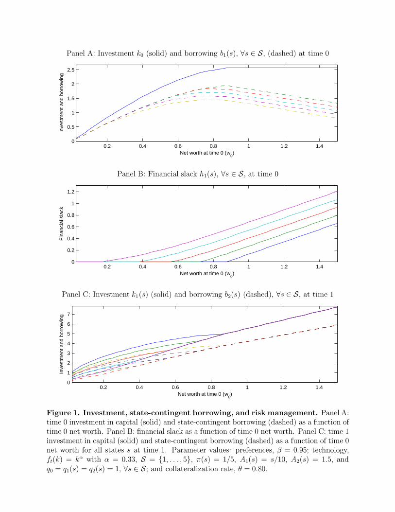
Panel A: Investment k0 (solid) and borrowing b1(s), ∀s ∈ S, (dashed) at time 0

0.2 0.4 0.6 0.8 1 1.2 1.40

0.5

1

1.5

2

2.5

Net worth at time 0 (w0)

Inve

stm

ent a

nd b

orro

win

g

Panel B: Financial slack h1(s), ∀s ∈ S, at time 0

0.2 0.4 0.6 0.8 1 1.2 1.40

0.2

0.4

0.6

0.8

1

1.2

Net worth at time 0 (w0)

Fin

anci

al s

lack

Panel C: Investment k1(s) (solid) and borrowing b2(s) (dashed), ∀s ∈ S, at time 1

0.2 0.4 0.6 0.8 1 1.2 1.40

1

2

3

4

5

6

7

Net worth at time 0 (w0)

Inve

stm

ent a

nd b

orro

win

g

Figure 1. Investment, state-contingent borrowing, and risk management. Panel A:time 0 investment in capital (solid) and state-contingent borrowing (dashed) as a function oftime 0 net worth. Panel B: financial slack as a function of time 0 net worth. Panel C: time 1investment in capital (solid) and state-contingent borrowing (dashed) as a function of time 0net worth for all states s at time 1. Parameter values: preferences, β = 0.95; technology,ft(k) = kα with α = 0.33, S = {1, . . . , 5}, π(s) = 1/5, A1(s) = s/10, A2(s) = 1.5, andq0 = q1(s) = q2(s) = 1, ∀s ∈ S; and collateralization rate, θ = 0.80.

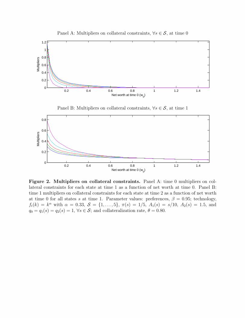
Panel A: Multipliers on collateral constraints, ∀s ∈ S, at time 0

0.2 0.4 0.6 0.8 1 1.2 1.40

0.2

0.4

0.6

0.8

1

1.2

Net worth at time 0 (w0)

Mul

tiplie

rs

Panel B: Multipliers on collateral constraints, ∀s ∈ S, at time 1

0.2 0.4 0.6 0.8 1 1.2 1.40

0.2

0.4

0.6

0.8

Net worth at time 0 (w0)

Mul

tiplie

rs

Figure 2. Multipliers on collateral constraints. Panel A: time 0 multipliers on col-lateral constraints for each state at time 1 as a function of net worth at time 0. Panel B:time 1 multipliers on collateral constraints for each state at time 2 as a function of net worthat time 0 for all states s at time 1. Parameter values: preferences, β = 0.95; technology,ft(k) = kα with α = 0.33, S = {1, . . . , 5}, π(s) = 1/5, A1(s) = s/10, A2(s) = 1.5, andq0 = q1(s) = q2(s) = 1, ∀s ∈ S; and collateralization rate, θ = 0.80.

0 1 2

������������

PPPPPPPPPPPP

s = H : µ1(H)

s = L: µ1(L)

π(H)

π(L) ��

No need forfinancing

Complete hedging: µ1(H) = µ1(L)

Figure 3. Risk management as in Froot, Scharfstein, and Stein (1993). Withcomplete markets, perfect enforcement at time 1, and no financing need at time 0, theoptimal hedging policy equalizes the marginal value of net worth µ1(s) across states attime 1.

0 1 2

������������

PPPPPPPPPPPP

s = H : µ1(H)

s = L: µ1(L)

π(H)

π(L)

��@@

µ0 = Rµ1(L) + Rλ1(L)

µ0 = Rµ1(H) + Rλ1(H)

I

Financing needfor investment

No hedging: µ1(H) 6= µ1(L)µ0

Figure 4. Financing and risk management subject to collateral constraints. Withcomplete markets subject to collateral constraints and a financing need at time 0, financingneeds may override hedging concerns, as the figure illustrates; in this case the optimal hedgingpolicy equalizes the sum of the marginal value of net worth and the multiplier on the collateralconstraint, µ1(s) + λ1(s), across states at time 1, as µ0 = Rµ1(s) + Rλ1(s), ∀s ∈ S, fromequation (A4).