Collateral and Capital Structure - Fuqua School of Businessrampini/papers/capitalstructure.pdf ·...
59
Collateral and Capital Structure Adriano A. Rampini * S. Viswanathan Duke University, Fuqua School of Business, 100 Fuqua Drive, Durham, NC, 27708, USA This draft January 2013; forthcoming, Journal of Financial Economics Abstract We develop a dynamic model of investment, capital structure, leasing, and risk management based on firms’ need to collateralize promises to pay with tangible assets. Both financing and risk management involve promises to pay subject to collateral constraints. Leasing is strongly collateralized costly financing and permits greater leverage. More constrained firms hedge less and lease more, both cross-sectionally and dynamically. Mature firms suffering adverse cash flow shocks may cut risk management and sell and lease back assets. Persistence of productivity reduces the benefits to hedging low cash flows and can lead firms not to hedge at all. JEL classification: D24; D82; E22; G31; G32; G35 Keywords: Collateral; Capital structure; Investment; Risk management; Leasing; Tangible capital; Intangible capital We thank Michael Brennan, Francesca Cornelli, Andrea Eisfeldt, Michael Fishman, Piero Gottardi, Dmitry Livdan, Ellen McGrattan, Lukas Schmid, Ilya Strebulaev, Tan Wang, Stan Zin, an anonymous referee, and seminar participants at Duke University, the Federal Reserve Bank of New York, the Toulouse School of Economics, the University of Texas at Austin, New York University, Boston University, MIT, Virginia, UCLA, Michigan, Washington University, McGill, Indiana, Koc, Lausanne, Yale, Amsterdam, Emory, the 2009 Finance Summit, the 2009 NBER Corporate Finance Program Meeting, the 2009 SED Annual Meeting, the 2009 CEPR European Summer Symposium in Financial Markets, the 2010 AEA Annual Meeting, the 2010 UBC Winter Finance Conference, the IDC Caesarea Center Conference, the 2010 FIRS Conference, the 2010 Econometric Society World Congress, and the 2011 AFA Annual Meeting for helpful comments and Sophia Zhengzi Li for research assistance. * Corresponding author. Tel: +1 919 660 7797; fax: +1 919 660 8038. E-mail address: [email protected] (Adriano A. Rampini).
Transcript of Collateral and Capital Structure - Fuqua School of Businessrampini/papers/capitalstructure.pdf ·...

Collateral and Capital Structure ?
Adriano A. Rampini ∗ S. Viswanathan
Duke University, Fuqua School of Business, 100 Fuqua Drive, Durham, NC, 27708, USA
This draft January 2013; forthcoming, Journal of Financial Economics
Abstract
We develop a dynamic model of investment, capital structure, leasing, and risk managementbased on firms’ need to collateralize promises to pay with tangible assets. Both financing and
risk management involve promises to pay subject to collateral constraints. Leasing is stronglycollateralized costly financing and permits greater leverage. More constrained firms hedge
less and lease more, both cross-sectionally and dynamically. Mature firms suffering adversecash flow shocks may cut risk management and sell and lease back assets. Persistence ofproductivity reduces the benefits to hedging low cash flows and can lead firms not to hedge
at all.
JEL classification: D24; D82; E22; G31; G32; G35
Keywords: Collateral; Capital structure; Investment; Risk management; Leasing; Tangiblecapital; Intangible capital
? We thank Michael Brennan, Francesca Cornelli, Andrea Eisfeldt, Michael Fishman, PieroGottardi, Dmitry Livdan, Ellen McGrattan, Lukas Schmid, Ilya Strebulaev, Tan Wang, Stan
Zin, an anonymous referee, and seminar participants at Duke University, the Federal ReserveBank of New York, the Toulouse School of Economics, the University of Texas at Austin, New
York University, Boston University, MIT, Virginia, UCLA, Michigan, Washington University,McGill, Indiana, Koc, Lausanne, Yale, Amsterdam, Emory, the 2009 Finance Summit, the
2009 NBER Corporate Finance Program Meeting, the 2009 SED Annual Meeting, the 2009CEPR European Summer Symposium in Financial Markets, the 2010 AEA Annual Meeting,
the 2010 UBC Winter Finance Conference, the IDC Caesarea Center Conference, the 2010FIRS Conference, the 2010 Econometric Society World Congress, and the 2011 AFA Annual
Meeting for helpful comments and Sophia Zhengzi Li for research assistance.∗ Corresponding author. Tel: +1 919 660 7797; fax: +1 919 660 8038.
E-mail address: [email protected] (Adriano A. Rampini).

1. Introduction
We argue that collateral determines the capital structure and develop a dynamic
agency based model of firm financing based on the need to collateralize promises to
pay with tangible assets. We maintain that the enforcement of payments is a critical
determinant of both firm financing and whether asset ownership resides with the user
or the financier, i.e., whether firms purchase or lease assets. We study a dynamic neo-
classical model of the firm in which financing is subject to collateral constraints derived
from limited enforcement and firms choose between purchasing and renting assets. Our
theory of optimal investment, capital structure, leasing, and risk management enables
the first dynamic analysis of the financing vs. risk management trade-off and of firm
financing when firms can rent capital.
In the frictionless neoclassical model asset ownership is indeterminate and firms are
assumed to rent all capital. The recent dynamic agency models of firm financing ignore
the possibility that firms rent capital. Of course, a frictionless rental market for capital
would obviate financial constraints. We explicitly consider firms’ dynamic lease vs. buy
decision, modeling leasing as highly collateralized albeit costly financing. When capital
is leased, the financier retains ownership which facilitates repossession and strengthens
the collateralization of the financier’s claim. Leasing is costly since the lessor incurs
monitoring costs to avoid agency problems due to the separation of ownership and
control.
We provide a definition of the user cost of capital in our model of investment with
financial constraints that is similar in spirit to Jorgenson’s (1963) definition in the
frictionless neoclassical model. Our user cost of capital is the sum of Jorgenson’s user
cost and a term which captures the additional cost due to the scarcity of internal funds.
In our model, firms require both tangible and intangible capital, but the enforcement
constraints imply that only tangible capital can be pledged as collateral and borrowed
against, resulting in a premium on internal funds; tangibility restricts external financing
and hence leverage.
There is a fundamental connection between the optimal financing and risk manage-
ment policy that has not been previously recognized. Both financing and risk manage-
ment involve promises to pay by the firm, leading to a trade off when such promises are
limited by collateral constraints. Indeed, firms with sufficiently low net worth do not
engage in risk management at all because the need to finance investment overrides the
hedging concerns. This result is in contrast to the extant theory, such as Froot, Scharf-
stein, and Stein (1993), and is consistent with the evidence that more constrained firms
hedge less provided by Rampini, Sufi, and Viswanathan (2012), and the literature cited
1

therein, and with the strong positive relation between hedging and firm size in the data.
With constant investment opportunities, risk management depends only on firms’ net
worth and incomplete hedging is optimal, i.e., firms do not hedge to the point where
the marginal value of net worth is equated across all states. In fact, firms abstain from
risk management with positive probability under the stationary distribution. Thus,
even mature firms that suffer a sequence of adverse cash flow shocks may see their net
worth decline to the point where they find it optimal to discontinue risk management.
We moreover characterize the comparative statics of firms’ investment, financing, risk
management, and dividend policy with respect to other key parameters of the model.
Firms subject to higher risk can choose to hedge more and reduce investment due to the
financing needs for risk management. Firms with more collateralizable or tangible assets
can lever more and increase investment, while at the same time raising corporate risk
management to counterbalance the increase in the volatility of net worth that higher
leverage would otherwise imply. Firms with more curvature in their production function
operate at smaller scale and may hence hedge less, not more as one might expect. Thus,
our model has interesting empirical implications for firm financing and risk management
both in the cross section and the time series.
With stochastic investment opportunities, risk management depends not only on
firms’ net worth but also on their productivity. If productivity is persistent, the overall
level of risk management is reduced, because cash flows and investment opportunities
are positively correlated due to the positive correlation between current productivity
and future expected productivity. There is less benefit to hedging low cash flow states.
Moreover, risk management is lower when current productivity is high, as higher ex-
pected productivity implies higher investment and raises the opportunity cost of risk
management. With sufficient but empirically plausible levels of persistence, the firm
abstains from risk management altogether, providing an additional reason why risk
management is so limited in practice. Furthermore, when the persistence of productiv-
ity is strong, firms hedge investment opportunities, i.e., states with high productivity,
as the financing needs for increased investment rise more than cash flows.
Leasing tangible assets requires less net worth per unit of capital and hence allows
firms to borrow more. Financially constrained firms, i.e., firms with low net worth, lease
capital because they value the higher debt capacity; indeed, severely constrained firms
lease all their tangible capital. Over time, as firms accumulate net worth, they grow in
size and start to buy capital. Thus, the model predicts that small firms and young firms
lease capital. We show that the ability to lease capital enables firms to grow faster.
Dynamically, mature firms that are hit by a sequence of low cash flows may sell assets
and lease them back, i.e., sale-leaseback transactions may occur under the stationary
2

distribution. Moreover, leasing has interesting implications for risk management: leasing
enables high implicit leverage; this may lead firms to engage in risk management to
reduce the volatility of net worth that such high leverage would otherwise imply.
In the data, we show that tangible assets are a key determinant of firm leverage.
Leverage varies by a factor 3 from the lowest to the highest tangibility quartile for
Compustat firms. Moreover, tangible assets are an important explanation for the “low
leverage puzzle” in the sense that firms with low leverage are largely firms with few
tangible assets. We also take firms’ ability to deploy tangible assets by renting or leasing
such assets into account. We show that accounting for leased assets in the measurement
of leverage and tangibility reduces the fraction of low leverage firms drastically and
that firms with low lease adjusted leverage are firms with low lease adjusted tangible
assets. Finally, we show that accounting for leased capital has a striking effect on the
relation between leverage and size in the cross section of Compustat firms. This relation
is essentially flat when leased capital is taken into account. In contrast, when leased
capital is ignored, as is done in the literature, leverage increases in size, i.e., small firms
seem less levered than large firms. Thus, basic stylized facts about the capital structure
need to be revisited. Importantly, the lease adjustments to the capital structure we
propose based on our theory are common in practice, and accounting rule changes are
currently being considered by the US and international accounting boards that would
result in the implementation of lease adjustments similar to ours throughout financial
accounting. Our model and empirical evidence together suggest a collateral view of the
capital structure.
Our paper is part of a recent and growing literature which considers dynamic incentive
problems as the main determinant of the capital structure. The incentive problem in our
model is limited enforcement of claims. Most closely related to our work are Albuquerque
and Hopenhayn (2004), Lorenzoni and Walentin (2007), and Rampini and Viswanathan
(2010). Albuquerque and Hopenhayn (2004) study dynamic firm financing with limited
enforcement. In their setting, the value of default is exogenous, albeit with fairly general
properties, whereas in our model the value of default is endogenous as firms are not
excluded from markets following default. Moreover, they do not consider the standard
neoclassical investment problem. 1 Lorenzoni and Walentin (2007) consider limits on
enforcement similar to ours in a model with constant returns to scale and adjustment
costs on aggregate investment which implies that all firms are equally constrained at any
given time. However, they assume that all enforcement constraints always bind, which
1 The aggregate implications of firm financing with limited enforcement are studied by Cooley,
Marimon, and Quadrini (2004) and Jermann and Quadrini (2007). Schmid (2008) considers
the quantitative implications for the dynamics of firm financing.
3

is not the case in our model, and focus on the relation between investment and Tobin’s
q rather than the capital structure. Rampini and Viswanathan (2010) consider a two
period model in a similar setting with heterogeneity in firm productivities and focus
on the distributional implications of limited risk management. While they consider the
comparative statics with respect to exogenously given initial net worth, net worth is
endogenously determined in our fully dynamic model, and our model moreover allows
the analysis of the dynamics of risk management, risk management by mature firms in
the long run, and the effect of persistence on the extent of risk management. Rampini,
Sufi, and Viswanathan (2012) extend the model in this paper to analyze the hedging of
a stochastic input price, e.g., airlines’ risk management of fuel prices.
The rationale for risk management in our model is related to the one in Froot, Scharf-
stein, and Stein (1993) who show that firms subject to financial constraints are effec-
tively risk averse and hence engage in risk management. Holmstrom and Tirole (2000)
recognize that financial constraints may limit ex ante risk management. Mello and Par-
sons (2000) also argue that financial constraints can restrict hedging. None of these
papers provide a dynamic analysis of the financing vs. risk management trade-off. 2
A literature, e.g., Leland (1998), argues that “[h]edging permits greater leverage” by
allowing firms to avoid bankruptcy costs when they are financed with non-contingent
debt. To the extent that low net worth firms have high leverage and a high probability
of bankruptcy, this implies a negative relation between net worth and risk management,
which is the opposite of our prediction and the relation in the data.
Capital structure and investment dynamics determined by incentive problems due to
private information about cash flows or moral hazard are studied by Quadrini (2004),
Clementi and Hopenhayn (2006), DeMarzo and Fishman (2007a), Biais, Mariotti, Ro-
chet, and Villeneuve (2010), and DeMarzo, Fishman, He, and Wang (2012). Capital
structure dynamics subject to similar incentive problems but abstracting from invest-
ment decisions are analyzed by DeMarzo and Fishman (2007b), DeMarzo and Sannikov
(2006), and Biais, Mariotti, Plantin, and Rochet (2007). 3 In these models, collateral
2 Bolton, Chen, and Wang (2011) study risk management in a neoclassical model of corporate
cash management; in contrast to our theory, they find that the hedge ratio decreases in firms’
cash-to-capital ratio, and low cash firms hedge as much as possible while high cash firms do
not hedge at all. The cost of hedging they consider is an inconvenience yield of posting cash to
meet an exogenous margin requirement rather than the financing risk management trade-off
we emphasize.3 Relatedly, Gromb (1995) analyzes a multi-period version of Bolton and Scharfstein (1990)’s
two period dynamic firm financing problem with privately observed cash flows. Gertler (1992)
considers the aggregate implications of a multi-period firm financing problem with privately
4

plays no role.
The role of secured debt is also considered in a literature which takes the form of
debt and equity claims as given. Stulz and Johnson (1985) argue that secured debt can
facilitate follow-on investment and thus ameliorate a Myers (1977) type underinvest-
ment problem in the presence of debt overhang. 4 Morellec (2001) shows that secured
debt prevents equityholders from liquidating assets to appropriate value from debthold-
ers. Using an incomplete contracting approach, Bolton and Oehmke (2012) analyze the
optimal priority structure between derivatives used for risk management and debt.
Several papers study the capital structure implications of agency conflicts due to
managers’ private benefits. Zwiebel (1996) argues that managers voluntarily choose
debt to credibly constrain their own future empire-building in a model with incomplete
contracts. Morellec, Nikolov, and Schurhoff (2012) study agency conflicts in a Leland
(1998) type model in which managers divert a part of cash flows as private benefits
leading them to lever less.
Moreover, none of these models consider intangible capital or the option to lease
capital. An exception is Eisfeldt and Rampini (2009) who argue that leasing amounts
to a particularly strong form of collateralization due to the relative ease with which
leased capital can be repossessed, albeit in a static model. We are the first, to the best
of our knowledge, to consider the role of leased capital in a dynamic model of firm
financing and provide a dynamic theory of sale-and-leaseback transactions.
In Section 2 we report some stylized empirical facts about collateralized financing,
tangibility, and leverage, taking leased capital into account. Section 3 describes the
model, defines the user cost of tangible, intangible, and leased capital, and characterizes
the payout policy. Section 4 analyzes optimal risk management and provides compara-
tive statics with respect to key parameters. Section 5 characterizes the optimal leasing
and capital structure policy and Section 6 concludes. All proofs are in Appendix A.
2. Stylized facts
This section provides some aggregate and cross-sectional evidence that highlights
the first order importance of tangible assets as a determinant of the capital structure
in the data. We first take an aggregate perspective and then document the relation
between tangible assets and leverage across firms. We take leased capital into account
observed cash flows. Atkeson and Cole (2008) consider a two period firm financing problem
with costly monitoring of cash flows.4 Hackbarth and Mauer (2012) provide a Leland (1994) type model where priority rules
mitigate this underinvestment problem.
5

explicitly and show that it has quantitatively and qualitatively large effects on basic
stylized facts about the capital structure, such as the relation between leverage and size.
Tangibility also turns out to be one of the few robust factors explaining firm leverage
in the extensive empirical literature on capital structure, but we do not attempt to
summarize this literature here.
2.1. Collateralized financing: the aggregate perspective
From the aggregate point of view, the importance of tangible assets is striking. Con-
sider the balance sheet data from the Flow of Funds Accounts of the U.S. for (nonfi-
nancial) corporate businesses, (nonfinancial) noncorporate businesses, and households
reported in Table 1 for the years 1999 to 2008 (detailed definitions of variables are in the
caption of the table). For businesses, tangible assets include real estate, equipment and
software, and inventories, and for households mainly real estate and consumer durables.
Panel A documents that from an aggregate perspective, the liabilities of corporate and
noncorporate businesses and households are less than their tangible assets and indeed
typically considerably less, and in this sense all liabilities are collateralized. For corpo-
rate businesses, debt in terms of credit market instruments is 48.5% of tangible assets.
Even total liabilities, which include also miscellaneous liabilities and trade payables, are
only 83.0% of tangible assets. For noncorporate businesses and households, liabilities
vary between 37.8% and 54.9% of tangible assets and are remarkably similar for the
two sectors.
Note that we do not consider whether liabilities are explicitly collateralized or only
implicitly in the sense that firms have tangible assets exceeding their liabilities. Our
reasoning is that even if liabilities are not explicitly collateralized, they are implic-
itly collateralized since restrictions on further investment, asset sales, and additional
borrowing through covenants and the ability not to refinance debt allow lenders to ef-
fectively limit borrowing to the value of collateral in the form of tangible assets. That
said, households’ liabilities are largely explicitly collateralized. Households’ mortgages,
which make up the bulk of households’ liabilities, account for 41.2% of the value of real
estate, while consumer credit amounts to 56.1% of the value of households’ consumer
durables.
Finally, aggregating across all balance sheets and ignoring the rest of the world im-
plies that tangible assets make up 79.2% of the net worth of U.S. households, with real
estate making up 60.2%, equipment and software 8.3%, and consumer durables 7.6%
(see Panel B). While this provides a coarse picture of collateral, it highlights the quan-
titative importance of tangible assets as well as the relation between tangible assets and
liabilities in the aggregate.
6

2.2. Tangibility and leverage
To document the relation between tangibility and leverage, we analyze data for a
cross section of Compustat firms. We sort firms into quartiles by tangibility measured
as the value of property, plant, and equipment divided by the market value of assets. The
results are reported in Panel A of Table 2, which also provides a detailed description of
the construction of the variables. We measure leverage as long term debt to the market
value of assets.
The first observation that we want to stress is that across tangibility quartiles, (me-
dian) leverage varies from 7.4% for low tangibility firms (i.e., firms in the lowest quartile)
to 22.6% for high tangibility firms (i.e., firms in the highest quartile), i.e., by a factor
3. Tangibility also varies substantially across quartiles; the cut-off value for the first
quartile is 6.3% and for the fourth quartile is 32.2%.
To assess the role of tangibility as an explanation for the observation that some firms
have very low leverage (the so-called “low leverage puzzle”), we compute the fraction of
firms in each tangibility quartile which have low leverage, specifically leverage less than
10%. The fraction of firms with low leverage decreases from 58.3% in the low tangibility
quartile to 14.9% in the high tangibility quartile. Thus, low leverage firms are largely
firms with relatively few tangible assets.
2.3. Leased capital and leverage
Thus far, we have ignored leased capital which is the conventional approach in the
literature. To account for leased (or rented) capital, we simply capitalize the rental
expense (Compustat item #47). This allows us to impute capital deployed via operating
leases, which are the bulk of leasing in practice. 5 To capitalize the rental expense, recall
that Jorgenson’s (1963) user cost of capital is u ≡ r + δ, i.e., the user cost is the sum
of the interest cost and the depreciation rate. Thus, the frictionless rental expense for
an amount of capital k is
Rent = (r + δ)k.
Given data on rental payments, we can hence infer the amount of capital rented by
capitalizing the rental expense using the factor 1/(r + δ). For simplicity, we capitalize
the rental expense by a factor 10. We adjust firms’ assets, tangible assets, and liabilities
by adding 10 times rental expense to obtain measures of lease adjusted assets, lease
5 Note that capital leases are already accounted for as they are capitalized on the balance
sheet for accounting purposes. For a description of the specifics of leasing in terms of the law,
accounting, and taxation see Eisfeldt and Rampini (2009) and the references cited therein.
7
adjusted tangible assets, and lease adjusted leverage. 6
We proceed as before and sort firms into quartiles by lease adjusted tangibility. The
results are reported in Panel B of Table 2. Lease adjusted debt leverage is somewhat
lower as we divide by lease adjusted assets here. There is a strong relation between
lease adjusted tangibility and lease adjusted leverage (as before), with the median lease
adjusted debt leverage varying again by a factor of about 3. Rental leverage also in-
creases with lease adjusted tangibility by about a factor 2 for the median and more
than 3 for the mean. Similarly, lease adjusted leverage, which we define as the sum of
debt leverage and rental leverage, also increases with tangibility by a factor 3.
Taking rental leverage into account reduces the fraction of firms with low leverage
drastically, in particular for firms outside the low tangibility quartile. Lease adjusted
tangibility is an even more important explanation for the “low leverage puzzle.” Indeed,
less than 4% of firms with high tangibility have low lease adjusted leverage.
It is also worth noting that the median rental leverage is on the order of half of
debt leverage or more, and is hence quantitatively important. Overall, we conclude that
tangibility, when adjusted for leased capital, emerges as a key determinant of leverage
and the fraction of firms with low leverage.
2.4. Leverage and size revisited
Considering leased capital changes basic cross-sectional properties of the capital struc-
ture. Here we document the relationship between firm size and leverage (see Table 3
and Fig. 1). We sort Compustat firms into deciles by size. We measure size by lease ad-
justed assets here, although using unadjusted assets makes our results even more stark.
Debt leverage is increasing in size, in particular for small firms, when leased capital is
ignored. Rental leverage, by contrast, decreases in size, in particular for small firms. 7
Indeed, rental leverage is substantially larger than debt leverage for small firms. Lease
adjusted leverage, i.e., the sum of debt and rental leverage, is roughly constant across
Compustat size deciles. In our view, this evidence provides a strong case that leased
capital cannot be ignored if one wants to understand the capital structure.
6 In accounting this approach to capitalization is known as constructive capitalization and
is frequently used in practice, with “8 x rent” being the most commonly used. E.g., Moody’s
rating methodology uses multiples of 5x, 6x, 8x, and 10x current rent expense, depending on
the industry. We discuss the calibration of the capitalization factor we use in footnote 12.7 Eisfeldt and Rampini (2009) show that this is even more dramatically the case in Census
data, which includes firms that are not in Compustat and hence much smaller, and argue that
for such firms renting capital may be the most important source of external finance.
8
3. Model
This section provides a dynamic agency based model to understand the first order
importance of tangible assets and rented assets for firm financing and the capital struc-
ture documented above. Dynamic financing is subject to collateral constraints due to
limited enforcement. We consider both tangible and intangible capital as well as firms’
ability to lease capital. Moreover, we define the user cost of tangible, intangible, and
leased capital. Finally, we characterize the dividend policy and show how tangibility
and collateralizability of assets affect the capital structure in the special case without
leasing.
3.1. Environment
A risk neutral firm subject to limited liability discounts the future at rate β ∈ (0, 1)
and requires financing for investment. The firm’s problem has an infinite horizon and
we write the problem recursively. The firm starts the period with net worth w and has
access to a standard neoclassical production function with decreasing returns to scale.
There are two types of capital, tangible capital and intangible capital. Tangible capital
can be either purchased (kp) or leased (kl), while intangible capital (ki) can only be
purchased. The total amount of capital is k ≡ ki + kp + kl and we refer to total capital
k often simply as capital. For simplicity, we assume that tangible and intangible capital
are required in fixed proportions and denote the fraction of tangible capital required
by ϕ. 8 Both tangible and intangible capital can be purchased at a price normalized
to 1 and depreciate at the same rate δ. There are no adjustment costs. An amount of
invested capital k yields stochastic cash flow A(s′)f(k) next period, where A(s′) is the
realized total factor productivity of the technology in state s′, which we assume follows
a Markov process described by the transition function Π(s, s′) on s′ ∈ S.
Tangible capital which the firm owns can be used as collateral for state-contingent
one period debt up to a fraction θ ∈ (0, 1) of its resale value. These collateral con-
straints are motivated by limited enforcement. We assume that enforcement is limited
8 We are implicitly using the Leontief aggregator of tangible and intangible capital min{(kp+
kl)/ϕ, ki/(1 − ϕ)} which yields ki = (1 − ϕ)k, kp + kl = ϕk, and k = ki + kp + kl as above,
simplifying the firm’s investment problem to the choice of capital k and leased capital kl
only. If tangible and intangible capital were not used in fixed proportions and had a constant
elasticity of substitution γ > −∞, i.e., the aggregator of tangible and intangible capital was
[σ(kp +kl)γ +(1−σ)kγ
i ]1/γ with γ ≤ 1, then the composition of capital would vary with firms’
financial condition, with more financially constrained firms using a lower fraction of intangible
capital.
9

in that firms can abscond with all cash flows, all intangible capital, and 1 − θ of pur-
chased tangible capital kp. Further we assume that firms cannot abscond with leased
capital kl, i.e., leased capital enjoys a repossession advantage. It is easier for a lessor,
who retains ownership of the asset, to repossess it, than for a secured lender, who only
has a security interest, to recover the collateral backing the loan. Leasing enjoys such
a repossession advantage under U.S. law and, we believe, in most legal systems. Im-
portantly, we assume that firms who abscond cannot be excluded from any market:
the market for intangible capital, tangible capital, loans, and rented capital. As we
show in Appendix B, these dynamic enforcement constraints imply the above collat-
eral constraints, which are similar to the ones in Kiyotaki and Moore (1997), albeit
state contingent, and are described in more detail below. 9 We emphasize that any
long-term contract that satisfies the enforcement constraints can be implemented with
such one-period ahead state contingent debt subject to the above collateral constraints
and hence long-term contracts are not ruled out. The motivation for our assumption
about the lack of exclusion is two-fold. First, it allows us to provide a tractable model
of dynamic collateralized firm financing. The equivalence of the two problems (with
limited enforcement and collateral constraints, respectively) enables us to work directly
with the problem with collateral constraints and use net worth as the state variable. In
contrast, the outside options considered in the literature result in continuation utility
being the appropriate state variable, which typically makes the dual problem easier to
work with (see, e.g., Albuquerque and Hopenhayn, 2004). Second, a model based on this
assumption has implications which are empirically plausible, in particular by putting
the focus squarely on tangibility.
We assume that intangible capital can neither be collateralized nor leased. The idea
is that intangible capital cannot be repossessed due to its lack of tangibility and can
be deployed in production only by the owner, since the agency problems involved in
separating ownership from control are too severe. 10
9 These collateral constraints are derived from an explictly dynamic model of limited en-
forcement similar to the one considered by Kehoe and Levine (1993). The main difference to
their limits on enforcement is that we assume that firms who abscond cannot be excluded
from future borrowing whereas they assume that borrowers are in fact excluded from in-
tertemporal trade after default. Similar constraints have been considered by Lustig (2007) in
an endowment economy, by Lorenzoni and Walentin (2007) in a production economy with
constant returns to scale, and by Rampini and Viswanathan (2010) in a production economy
with a finite horizon. Krueger and Uhlig (2006) find that similar limits on enforcement in an
endowment economy without collateral imply short-sale constraints, which would be true in
our model in the special case where θ = 0.10 The assumption that intangible capital cannot be collateralized or leased at all simplifies
10

Our model considers the role of leased capital in a dynamic model of firm financing
subject to limited enforcement. The assumption that firms cannot abscond with leased
capital captures the fact that leased capital can be repossessed more easily. This repos-
session advantage means that by leasing the firm can effectively borrow against the full
resale value of tangible assets, whereas secured lending allows the firm to borrow only
against a fraction θ of the resale value. The benefit of leasing is its higher debt capacity.
However, leasing also has a cost: leased capital involves monitoring costs m per unit of
capital incurred by the lessor at the end of the period, which are reflected in the user
cost of leased capital ul. Leasing separates ownership and control and the lessor must
pay the cost m to ensure that the lessee uses and maintains the asset appropriately. 11
A competitive lessor with a cost of capital R ≡ 1 + r charges a user cost of
ul ≡ r + δ + m
per unit of capital. Equivalently, we could assume that leased capital depreciates faster
due to the agency problem at rate δl > δ and set m = δl − δ. Due to the constraints on
enforcement, the user cost of leased capital is charged at the beginning of the period
and hence the firm pays R−1ul per unit of leased capital up front. Specifically, since
the lessor recovers the leased capital at the end of the period, no additional payments
at the end of the period can be enforced and the leasing fee must hence be charged
up front. Recall that in the frictionless neoclassical model, the rental cost of capital is
Jorgenson (1963)’s user cost u ≡ r + δ. Thus the only difference to the rental cost in
our model is the positive monitoring cost m (or, equivalently, the costs due to faster
depreciation δl − δ). Note that as in Jorgenson’s definition, we define the user cost of
capital in terms of value at the end of the period. 12
the analysis, but is not required for the main results. Assuming that intangible capital is less
collateralizable and more costly to lease would suffice.11 In practice, there may be a link between the lessor’s monitoring and the repossession ad-
vantage of leasing. In order to monitor the use and maintenance of the asset, the lessor needs
to keep track of the asset which makes it harder for the lessee to abscond with it.12 To impute the amount of capital rented from rental payments, we should hence capitalize
rental payments by 1/(R−1(r + δ + m)). In documenting the stylized facts, we assumed that
this factor takes a value of 10. This calibrated value is based on an approximate (unlevered)
real cost of capital for tangible assets of 4%, an approximate depreciation rate for leased
tangible assets of 5% (using a depreciation rate of 3% for structures and 15% for equipment,
which are based on BEA data, and a weight of 80% (20%) on structures (equipment), since
leased tangible assets are predominantly structures and structures are 66% of non-residential
fixed assets overall), and an assumed monitoring cost m of 1%. The implicit debt associated
with rented capital is R−1(1−δ) times the amount of capital rented, so in adjusting liabilities,
11
We assume that the firm has access to lenders who have deep pockets in all dates and
states and discount the future at rate R−1 ∈ (β, 1). These lenders are thus willing to
lend in a state-contingent way at an expected return R. The assumption that firms are
less patient than lenders, which is quite common, 13 implies that firms’ financing policy
matters even in the long run, i.e., even for mature firms, and that the financing policy
is uniquely determined. Moreover, firms are never completely unconstrained and firms
which currently pay dividends that are hit by a sequence of low cash flow shocks may
eventually stop dividend payments, cut risk management, and switch back to leasing
capital, implications that are empirically plausible. 14
Firms in our model thus have access to two sources of external financing, state-
contingent secured debt and leasing. In Section 4 we provide an alternative interpre-
tation, which is equivalent, in which firms have access to non-contingent secured debt,
leasing, and risk management using one period ahead Arrow securities subject to short
sale constraints.
3.2. Firm’s problem
The firm’s problem can be written recursively as the problem of maximizing the
discounted expected value of future dividends by choosing the current dividend d, capital
k, leased capital kl, net worth w(s′) in state s′ next period, and state-contingent debt
b(s′) given current net worth w and state s:
V (w, s) ≡ max{d,k,kl ,w(s′),b(s′)}∈R
3+S+
×RS
d + β∑
s′∈S
Π(s, s′)V (w(s′), s′) (1)
subject to the budget constraints for the current and next period
w +∑
s′∈S
Π(s, s′)b(s′)≥ d + (k − kl) + R−1ulkl (2)
A(s′)f(k) + (k − kl)(1 − δ)≥w(s′) + Rb(s′), ∀s′ ∈ S, (3)
we should adjust by R−1(1− δ) times 10 to be precise. In documenting the stylized facts, we
ignored the correction R−1(1 − δ), implicitly assuming that it is approximately equal to 1.13 E.g., this assumption is made by DeMarzo and Sannikov (2006), Lorenzoni and Walentin
(2007), Biais, Mariotti, Plantin, and Rochet (2007), Biais, Mariotti, Rochet, and Villeneuve
(2010), and DeMarzo, Fishman, He, and Wang (2012); DeMarzo and Fishman (2007a, 2007b)
consider β ≤ R−1; in contrast, firms and lenders are assumed to be equally patient in Al-
buquerque and Hopenhayn (2004), Quadrini (2004), Clementi and Hopenhayn (2006), and
Rampini and Viswanathan (2010).14 While we do not explicitly consider taxes here, our assumption about discount rates can also
be interpreted as a reduced form way of taking into account the tax-deductibility of interest,
which effectively lowers the cost of debt finance.
12
the collateral constraints
θ(ϕk − kl)(1 − δ) ≥ Rb(s′), ∀s′ ∈ S, (4)
and the constraint that only tangible capital can be leased
ϕk ≥ kl. (5)
The program in (1)-(5) requires that dividends d and net worth w(s′) are non-negative
which is due to limited liability. Furthermore, capital k and leased capital kl have to be
non-negative as well. We write the budget constraints as inequality constraints, despite
the fact that they bind at an optimal contract, since this makes the constraint set
convex as shown below. There are only two state variables in this recursive formulation,
net worth w and the state of productivity s. This is due to our assumption that there
are no adjustment costs of any kind and greatly simplifies the analysis. Net worth in
state s′ next period w(s′) = A(s′)f(k)+(k−kl)(1−δ)−Rb(s′), i.e., equals cash flow plus
the depreciated resale value of owned capital minus the amount to be repaid on state s′
contingent debt. Borrowing against state s′ next period by issuing state s′ contingent
debt b(s′) reduces net worth w(s′) in that state. In other words, borrowing less than the
maximum amount which satisfies the collateral constraint (4) against state s′ amounts
to conserving net worth for that state and allows the firm to hedge the available net
worth in that state.
We make the following assumptions about the stochastic process describing produc-
tivity and the production function:
Assumption 1. For all s, s ∈ S such that s > s, (i) A(s) > A(s) and (ii) A(s) > 0.
Assumption 2. f is strictly increasing, strictly concave, f(0) = 0, limk→0 fk(k) =
+∞, and limk→+∞ fk(k) = 0.
We first show that the firm financing problem is a well-behaved dynamic programming
problem and that there exists a unique value function V which solves the problem.
To simplify notation, we introduce the shorthand for the choice variables x, where
x ≡ [d, k, kl, w(s′), b(s′)]′, and the shorthand for the constraint set Γ(w, s) given the
state variables w and s, defined as the set of x ∈ R3+S+ × R
S such that (2) to (5) are
satisfied. Define operator T as
(Tg)(w, s) = maxx∈Γ(w,s)
d + β∑
s′∈S
Π(s, s′)g(w(s′), s′).
We prove the following result about the firm financing problem in (1) to (5):
13

Proposition 1. (i) Γ(w, s) is convex, given (w, s), and convex in w and monotone in
the sense that w ≤ w implies Γ(w, s) ⊆ Γ(w, s). (ii) The operator T satisfies Blackwell’s
sufficient conditions for a contraction and has a unique fixed point V . (iii) V is con-
tinuous, strictly increasing, and concave in w. (iv) Without leasing, V (w, s) is strictly
concave in w for w ∈ int{w : d(w, s) = 0}. (v) Assuming that for all s, s ∈ S such
that s > s, Π(s, s′) strictly first order stochastically dominates Π(s, s′), V is strictly
increasing in s.
The proofs of part (i) to (iii) of the proposition are relatively standard. Part (iii) however
only states that the value function is concave, not strictly concave. The value function
is linear in net worth when dividends are paid. The value function may also be linear
in net worth on some intervals where no dividends are paid, due to the linearity of
the substitution between leased and owned capital. All our proofs below hence rely on
weak concavity only. Nevertheless we can show that without leasing, the value function
is strictly concave where no dividends are paid (see part (iv) of the proposition). 15
Denote the multipliers on the constraints (2) to (5) by µ, Π(s, s′)βµ(s′), Π(s, s′)βλ(s′),
and νl. Let νd and νl be the multipliers on the constraint d ≥ 0 and kl ≥ 0. The first
order conditions of the firm financing problem in Eqs. (1) to (5) are
µ =1 + νd (6)
µ =∑
s′∈S
Π(s, s′)β {µ(s′) [A(s′)fk(k) + (1 − δ)] + λ(s′)θϕ(1 − δ)} + νlϕ(7)
(1 − R−1ul)µ =∑
s′∈S
Π(s, s′)β {µ(s′)(1 − δ) + λ(s′)θ(1 − δ)} + νl − νl (8)
µ(s′)=Vw(w(s′), s′), ∀s′ ∈ S, (9)
µ =βµ(s′)R + βλ(s′)R, ∀s′ ∈ S, (10)
where we use the fact that the constraints k ≥ 0 and w(s′) ≥ 0, ∀s′ ∈ S, are slack as
Lemma 6 in Appendix A shows. 16 The envelope condition is Vw(w, s) = µ; the marginal
value of (current) net worth is µ. Similarly, the marginal value of net worth in state s′
next period is µ(s′).
15 Section 5 discusses how the linearity of the substitution between leased and owned capital
may result in intervals on which the value function is linear and shows that when m is suf-
ficiently high, the value function is strictly concave in the non-dividend paying region even
with leasing.16 Since the marginal product of capital is unbounded as capital goes to zero by Assumption 2,
capital is strictly positive. Because the firm’s ability to issue promises against capital is limited,
this in turn implies that the firm’s net worth is positive in all states next period.
14

Using Eqs. (7) and (10), we obtain the investment Euler equation,
1 ≥∑
s′∈S
Π(s, s′)βµ(s′)
µ
A(s′)fk(k) + (1 − θϕ)(1 − δ)
1 −R−1θϕ(1 − δ), (11)
which holds with equality if the firm does not lease all its tangible assets (i.e., νl = 0).
Notice that βµ(s′)/µ is the firm’s stochastic discount factor; collateral constraints render
the firm as if risk averse and hence provide a rationale for risk management.
3.3. User cost of capital
This section defines the user cost of (purchased) tangible and intangible capital in
the presence of collateral constraints extending Jorgenson’s (1963) definition. The def-
initions clarify the main economic intuition and allow a simple characterization of the
leasing decision as we show in Section 5.
Denote the premium on internal funds for a firm with net worth w in state s by ρ(w, s)
and define it implicitly using the firm’s stochastic discount factor as 1/(1+r+ρ(w, s)) ≡∑
s′∈S Π(s, s′)βµ(s′)/µ; internal funds command a premium as long as at least one of
the collateral constraints is binding. Define the user cost of tangible capital which is
purchased up(w, s) for a firm with net worth w in state s as
up(w, s) ≡ r + δ +ρ(w, s)
R + ρ(w, s)(1 − θ)(1 − δ) (12)
where ρ(w, s)/(R + ρ(w, s)) =∑
s′∈S Π(s, s′)Rβλ(s′)/µ. The user cost of purchased
tangible capital is the sum of the Jorgensonian user cost of capital and a second term,
which captures the additional cost of internal funds for the fraction (1 − θ)(1 − δ) of
capital that has to be financed internally. Analogously, the user cost of intangible capital
is ui(w, s) ≡ r + δ + ρ(w, s)/(R + ρ(w, s))(1 − δ).
Using our definitions, we can rewrite the first order condition for capital, Eq. (7), as
ϕmin{up(w, s), ul} + (1 − ϕ)ui(w, s) =∑
s′∈S
Π(s, s′)Rβµ(s′)
µA(s′)fk(k).
Optimal investment equates the weighted average of the user cost of tangible and in-
tangible capital with the expected marginal product of capital, where the applicable
user cost of tangible capital is the minimum of the user cost of purchased and leased
capital. 17
17 We can rewrite Eq. (12) in a weighted average (user) cost of capital form as up(w, s) =
R/(R+ρ(w, s))((r+ρ(w, s))[1−R−1θ(1−δ)]+r[R−1θ(1−δ)]+δ), where the fraction of capital
that can be financed externally, R−1θ(1− δ), is charged a cost of capital r, while the fraction
15

3.4. Dividend payout policy
We start by characterizing the firm’s payout policy. The firm’s dividend policy is very
intuitive: there is a state-contingent cutoff level of net worth w(s), ∀s ∈ S, above which
the firm pays dividends. 18 Moreover, whenever the firm has net worth w exceeding the
cutoff w(s), paying dividends in the amount w − w(s) is optimal. All firms with net
worth w exceeding the cutoff w(s) in a given state s, choose the same level of capital.
Finally, the investment policy is unique in terms of the choice of capital k. The following
proposition summarizes the characterization of firms’ payout policy:
Proposition 2 (Dividend policy) There is a state-contingent cutoff level of net worth,
above which the marginal value of net worth is one and the firm pays dividends: (i)
∀s ∈ S, ∃w(s) such that, ∀w ≥ w(s), µ(w, s) = 1. (ii) For ∀w ≥ w(s),
[do(w, s), ko(w, s), kl,o(w, s), wo(s′), bo(s
′)] = [w − w(s), ko(s), kl,o(s), wo(s′), bo(s
′)]
where xo ≡ [0, ko(s), kl,o(s), wo(s′), bo(s
′)] attains V (w(s), s). Indeed, ko(w, s) is unique
for all w and s. (iii) Without leasing, the optimal policy xo is unique.
3.5. Effect of tangibility and collateralizability without leasing
We distinguish between the fraction of tangible assets required for production, ϕ, and
the fraction of tangible assets θ that the borrower cannot abscond with and that is hence
collateralizable. This distinction is important to understand differences in the capital
structure across industries, as the fraction of tangible assets required for production
varies considerably at the industry level whereas the fraction of tangible assets that
is collateralizable primarily depends on the type of capital, such as structures versus
equipment (which we do not distinguish here). Thus, industry variation in ϕ needs to
be taken into account in empirical work. That said, in the special case without leasing,
higher tangibility ϕ and higher collateralizability θ are equivalent in our model. This
result is immediate as without leasing, ϕ and θ affect only (4) and only the product
of the two matters. Thus, firms that operate in industries that require more intangible
capital are more constrained, all else equal. Furthermore, the fact that firms can only
borrow against a fraction ϕθ of total capital is quantitatively relevant as the model
predicts much lower, and empirically plausible, leverage ratios.
that has to be financed internally, 1 − R−1θ(1 − δ), is charged a cost of capital r + ρ(w, s).18 Consistent with this prediction, DeAngelo, DeAngelo, and Stulz (2006) find a strong positive
relation between the probability that firms pay dividends and their retained earnings.
16

4. Risk management and the capital structure
Our model allows an explicit analysis of dynamic risk management since firms have
access to complete markets subject to the collateral constraints. We first show how
to interpret the state-contingent debt in our model in terms of risk management and
provide a general result about the optimal absence of risk management for firms with
sufficiently low net worth. Next, we prove the optimality of incomplete hedging with
constant investment opportunities, i.e., when productivity shocks are independently
and identically distributed; indeed, firms abstain from risk management with positive
probability under the stationary distribution, implying that even mature firms that
experience a sequence of low cash flows eliminate risk management. Moreover, with
stochastic investment opportunities persistent shocks further reduce risk management
and may result in a complete absence of risk management for empirically plausible levels
of persistence. Strong persistence of productivity may result in firms hedging higher
productivity states, because financing needs for increased investment rise more than
cash flows. Finally, we analyze the comparative statics of firms’ investment, financing,
risk management, and dividend policy with respect to key parameters of the model.
4.1. Optimal absence of risk management
Our model with state-contingent debt b(s′) is equivalent to a model in which firms
borrow as much as they can against each unit of tangible capital which they purchase,
i.e., borrow R−1θϕ(1 − δ) per unit of capital, and keep additional net worth in a state
contingent way by purchasing Arrow securities with a payoff of h(s′) for state s′. This
formulation allows us to characterize the corporate hedging policy. Specifically, we define
risk management in terms of purchases of Arrow securities for state s′ as
h(s′) ≡ θ(ϕk − kl)(1 − δ) − Rb(s′). (13)
We say a firm does not engage in risk management when the firm does not buy Arrow
securities for any state next period. Under this interpretation, firms’ debt is not state-
contingent and hence risk-free, as are lease contracts, since we assume that the price
of capital is constant for all states. We denote the amount firms pay down per unit of
capital by ℘(ϕ) ≡ 1−R−1θϕ(1−δ) and the amount firms pay down per unit of tangible
capital by ℘ ≡ ℘(1) ≡ 1 − R−1θ(1 − δ). Using this notation, we can write the budget
constraints for the current and next period (2) and (3) for this implementation as
w ≥ d +∑
s′∈S
Π(s, s′)R−1h(s′) + ℘(ϕ)k − (℘ − R−1ul)kl (14)
A(s′)f(k) + [(1 − ϕ)k + (1 − θ)(ϕk − kl)](1 − δ) + h(s′) ≥ w(s′), (15)
17

and the collateral constraints (4) reduce to short sale constraints
h(s′) ≥ 0, ∀s′ ∈ S, (16)
implying that holdings of Arrow securities have to be non-negative. The budget con-
straint (14) makes the trade-off between financing and risk management particularly
apparent; the firm can spend its net worth w on purchases of Arrow securities, i.e., hedg-
ing, or to buy fully levered capital; leasing frees up net worth as long as ℘−R−1ul > 0
which we assume (see Assumption 3 in Section 5) as leasing is otherwise dominated.
Eq. (15) states that net worth w(s′) in state s′ next period is the sum of cash flows, the
value of intangible capital and owned tangible capital not pledged to the lenders, and
the payoffs of the Arrow securities, if any. Our model with state-contingent borrowing
is hence a model of financing and risk management.
In the implementation considered in this section, firms pledge as much as they can
against their tangible assets to lenders leaving no collateral to pledge to derivatives
counterparties. The holdings of Arrow securities are hence subject to short sale con-
straints and the cost of risk management is the net worth required in the current
period to purchase them. That said, since firms in our model have access to complete
markets, subject to collateral constraints, firms can replicate any type of derivatives
contract, including forward contracts or futures that do not involve payments up front,
implying that our results hold for forward contracts and futures, too. Such contracts
involve promises to pay in some states next period which count against the collateral
constraints in those states. There is an opportunity cost for such promises, because
promises against these states could alternatively be used to finance current investment.
Thus, there are no constraints on the type of hedging instruments firms can use in our
model, and the only constraint on risk management is that promised payments need to
be collateralized, which is identical to the constraint imposed on financing.
The next proposition states that for severely constrained firms all collateral con-
straints bind, which means that such firms do not purchase any Arrow securities at
all, and, in this sense, do not engage in risk management. The numerical examples in
Sections 4.2 and 4.4 show that the extent to which firms hedge low states is in fact
increasing in net worth. 19
Severely constrained firms optimally abstain from risk management altogether:
19 In our model, we do not take a stand on whether the productivity shocks are firm specific
or aggregate. Since all states are observable, as the only friction considered is limited enforce-
ment, our analysis applies either way. Hedging can hence be interpreted either as using loan
commitments, e.g., to hedge idiosyncratic shocks to firms’ net worth or as using traded assets
to hedge aggregate shocks which affect firms’ cash flows.
18

Proposition 3 (Optimal absence of risk management) Firms with sufficiently low
net worth do not engage in risk management, i.e., ∀s ∈ S, ∃wh(s) > 0, such that
∀w ≤ wh(s), all collateral constraints bind, λ(s′) > 0, ∀s′ ∈ S.
Collateral constraints imply that there is an opportunity cost to issuing promises to pay
in high net worth states next period to hedge low net worth states, as such promises
can also be used to finance current investment. The proposition shows that when net
worth is sufficiently low, the opportunity cost of risk management due to the financing
needs must exceed the benefit. Hence, firms optimally do not hedge at all. Notice that
the result obtains for a general Markov process for productivity. The result is consistent
with the evidence that firms with low net worth hedge less, and is in contrast to the
conclusions from static models in the extant literature, such as Froot, Scharfstein, and
Stein (1993). The key difference is that our model explicitly considers dynamic financing
needs for investment as well as the limits on firms’ ability to promise to pay.
4.2. Risk management with constant investment opportunities
With independent productivity shocks, risk management only depends on the firm’s
net worth, because the expected productivity of capital is independent of the current
state s, i.e., investment opportunities are constant. More generally, both cash flows
and investment opportunities vary, and the correlation between the two affects the
desirability of hedging, as we show in Section 4.4 below.
With constant investment opportunities, the marginal value of net worth is higher in
states with low cash flows and complete hedging is never optimal:
Proposition 4 (Optimality of incomplete hedging) Suppose that Π(s, s′) = Π(s′),
∀s, s′ ∈ S. (i) The marginal value of net worth next period µ(s′) = Vw(w(s′)) is (weakly)
decreasing in the state s′, and the multipliers on the collateral constraints are (weakly)
increasing in the state s′, i.e., ∀s′, s′+ ∈ S such that s′+ > s′, µ(s′+) ≤ µ(s′) and
λ(s′+) ≥ λ(s′). (ii) Incomplete hedging is optimal, i.e., ∃s′ ∈ S, such that λ(s′) > 0.
Indeed, ∃s′, s′ ∈ S, such that w(s′) 6= w(s′). Moreover, the firm never hedges the highest
state, i.e., is always borrowing constrained against the highest state, λ(s′) > 0 where
s′ = max{s′ : s′ ∈ S}. The firm hedges a lower interval of states, [s′, . . . , s′h], where
s′ = min{s′ : s′ ∈ S}, if at all.
Complete hedging would imply that all collateral constraints are slack and consequently
the marginal value of net worth is equalized across all states next period. But hedging
involves conserving net worth in a state-contingent way at a return R. Given the firm’s
relative impatience, it can never be optimal to save in this state-contingent way for all
19

states next period. Thus, incomplete hedging is optimal. Further, since the marginal
value of net worth is higher in states with low cash flow realizations, it is optimal
to hedge the net worth in these states, if it is optimal to hedge at all. Firms’ optimal
hedging policy implicitly ensures a minimum level of net worth in all states next period.
We emphasize that our explicit dynamic model of collateral constraints due to limited
enforcement is essential for this result. If the firm’s ability to pledge were not limited,
then the firm would always want to pledge more against high net worth states next
period to equate net worth across all states. However, in our model the ability to
credibly pledge to pay is limited and there is an opportunity cost to pledging to pay
in high net worth states next period, since such pledges are also required for financing
current investment. This opportunity cost implies that the firm never chooses to fully
hedge net worth shocks.
To illustrate the interaction between financing needs and risk management, we com-
pute a numerical example. We assume that productivity is independent and, for sim-
plicity, that productivity takes on two values only, A(s1) < A(s2), and that there is no
leasing. The results and details of the parameterization are reported in Fig. 2.
Investment as a function of net worth is shown in Panel A, which illustrates Propo-
sition 2. Above a threshold w, firms pay dividends and investment is constant. Below
the threshold, investment is increasing in net worth and dividends are zero.
The dependence of risk management on net worth is illustrated in Panel B. With
independent shocks, the firm never hedges the high state, i.e., h(s′2) = 0, where h(s′) is
defined as in Eq. (13) (see Proposition 4). Panel B thus displays only the payoff of the
Arrow securities that the firm purchases to hedge the low state, h(s′1). Importantly, note
that the hedging policy is increasing in firm net worth, i.e., better capitalized firms hedge
more. This illustrates the main conclusion from our model for risk management. Above
the threshold w, hedging is constant (as Proposition 2 shows). Below the threshold,
hedging is increasing, and for sufficiently low values of net worth w, the firm does not
hedge at all, as Proposition 3 shows more generally. Indeed, hedging is zero for a sizable
range of values of net worth (up to a value of around 0.1 in the example).
The values of net worth next period are displayed in Panel C and illustrate the
endogenous dynamics of net worth. Since optimal hedging is incomplete, net worth
next period is higher in state s′2 than in state s′1. The figure moreover plots the 45
degree line (dotted), where w = w′, to facilitate the characterization of the dynamics of
net worth and the stationary distribution. Net worth next period is higher than current
net worth, i.e., increases, when w(s′) is above the 45 degree line and decreases otherwise.
In the low (high) state next period net worth decreases (increases) for all levels of net
worth above (below) the intersection of w(s′1) (w(s′2)) and the 45 degree line, which
20

we denote w(s1) (w(s2)). These transition dynamics of net worth together with the
policy functions describe the dynamics of investment, financing, and risk management
fully; if the low (high) state is realized, investment and risk management both decrease
(increase) as long as current net worth is in the interval [w(s1), w(s2)].
Since levels of net worth below w(s1) and above w(s2) are transient, the ergodic set
must be bounded below by w(s1) and above by w(s2), and the support of the stationary
distribution is a subset of the interval [w(s1), w(s2)]. Indeed, firms with net worth above
w(s2) will pay out the extra net worth and start the next period within the ergodic set.
Moreover, evaluating the first order condition (10) for b(s′) at w(s1) and s′ = s1, we
have Vw(w(s1)) = RβVw(w(s1)) + Rβλ(w(s1)) and thus λ(w(s1)) > 0. This means that
the firm abstains from risk management altogether at w(s1). By continuity, the absence
of risk management is optimal for sufficiently low values of net worth in the stationary
distribution, a result that is more generally true (see Proposition 5 below).
The multipliers on the collateral constraints λ(s′) are shown in Panel D. The first
order conditions (10) for b(s′) imply that µ(s′1) + λ(s′1) = µ(s′2) + λ(s′2); firms do not
simply equate the marginal value of net worth across states, but the sum of the marginal
value of net worth and the multiplier on the collateral constraint. The figure shows that
λ(s′2) > 0 for all w, whereas the multiplier on the collateral constraint for the low state
λ(s′1) is zero for levels of w at which the firm hedges and positive for lower levels at
which the firm abstains from risk management. Collateral constraints result in a trade
off between financing and risk management.
4.3. Risk management under the stationary distribution
We now show that firms do not hedge at the lower bound of the stationary distribution
as we observed in the example above. Indeed, firms abstain from risk management with
positive probability under the (unique) stationary distribution.
Proposition 5 (Absence of risk management under the stationary distribution)
Suppose Π(s, s′) = Π(s′), ∀s, s′ ∈ S, and m = +∞ (no leasing). (i) For the lowest state
s′, the wealth level w for which w(s′) = w is unique and the firm abstains from risk
management at w. (ii) There exists a unique stationary distribution of net worth and
firms abstain from risk management with positive probability under the stationary dis-
tribution.
Proposition 5 implies that even if a firm is currently relatively well capitalized and
paying dividends, a sufficiently long sequence of low cash flows will leave the firm so
21

constrained that it chooses to stop hedging. 20 Thus, it is not only young firms with very
low net worth that abstain from risk management, but also mature firms that suffer
adverse cash flow shocks. Consistently, Rampini, Sufi, and Viswanathan (2012) show
that airlines that hit financial distress dramatically cut their fuel price risk management.
4.4. Risk management with stochastic investment opportunities
With stochastic investment opportunities, risk management depends not only on net
worth but also on the firm’s productivity, since the conditional expectation of future
productivity varies with current productivity when productivity is persistent. Positive
autocorrelation reduces the benefit to hedging and can eliminate the need to hedge
completely.
We first show that incomplete hedging is optimal even when investment opportunities
are stochastic:
Proposition 6 (Optimality of incomplete hedging with persistence) Suppose m =
+∞ (no leasing). Optimal risk management is incomplete with positive probability, i.e.,
∃s such that for all w, λ(s′) > 0, for some s′.
Thus, firms engage in incomplete risk management for any Markov process of produc-
tivity, generalizing the results from Proposition 4. As in the case without persistence,
firms engage in risk management to transfer funds into states in which the marginal
value of net worth is highest (if at all). With persistence, however, the marginal value of
net worth depends on both net worth and investment opportunities going forward. Pos-
itive autocorrelation, which is typical in practice, implies that investment opportunities
are worse (better) when productivity is low (high), decreasing (increasing) the marginal
value of net worth in states with low (high) realizations. This reduces the benefit to
hedging and thus firms hedge less or not at all. Indeed, if this effect is strong enough,
firms may hedge states with high productivity, despite the fact that cash flows are high
then, too. Current investment opportunities also affect the benefits to investing and
the opportunity cost of hedging, and thus the extent of risk management depends on
current productivity as well.
To study the effect of persistence, we reconsider the example with a two state symmet-
ric Markov process for productivity from the previous section. The results are reported
in Fig. 3. We increase the transition probabilities Π(s1, s1) = Π(s2, s2) ≡ π, which are
20 Eq. (10) implies that there is an upper bound on the extent to which the marginal value
of net worth can increase as Vw(w(s′), s′)/Vw(w, s) ≤ (βR)−1; however, the marginal value of
net worth could increase, e.g., when cash flows are sufficiently low.
22

0.5 when investment opportunities are constant, progressively to 0.55, 0.60, 0.75, and
0.90. Since the autocorrelation of a symmetric two state Markov process is 2π − 1,
this corresponds to progressively raising the autocorrelation from 0 to 0.1, 0.2, 0.5, and
0.8. Given the symmetry, the stationary distribution of the productivity process over
the two states is 0.5 and 0.5 across all our examples, and the unconditional expected
productivity is hence the same as well.
Panels A and B display the investment and hedging policies in the case without
persistence from the previous section (see also Fig. 2). Since these policy functions are
independent of the state of productivity s, there is only one function for each policy. In
the panels with persistence, the solid lines denote the policies when current productivity
is low (s1) and the dashed lines the ones when current productivity is high (s2).
The left panels show that as persistence increases, investment is higher when current
productivity is high, because the conditional expected productivity is higher. The right
panels show the effect of persistence on the hedging policy. Panel D shows that hedging
(for the low state) decreases relative to the case without persistence, but more so when
current productivity is high. Most notably, for given net worth, the firm hedges the low
state less when current productivity is high than when it is low. The economic intuition
has two aspects. First, persistent shocks reduce the marginal value of net worth when
productivity is low (since the conditional expected productivity is low then too) while
raising the marginal value of net worth when productivity is high. Thus, there is less
reason to hedge. Second, high current productivity leads to higher investment when
productivity is persistent (and higher opportunity cost of risk management), which
raises net worth next period and further reduces the hedging need. This second effect
goes the other way when current productivity is low, but the first effect dominates in
our example even in this case.
When persistence is raised further, the benefit to hedging is still lower and the firm
abstains from hedging completely when current productivity is high and only hedges
(the low state) when current productivity is low (Panel F); indeed, the firm stops hedg-
ing completely at an autocorrelation of productivity of 0.5 (see Panel H). This suggests
that, for empirically plausible parameterizations (see, e.g., the calibrated autocorrela-
tion of 0.62 in Gomes, 2001), even firms with high net worth may engage in only limited
risk management or none at all.
For the persistence levels considered thus far, firms hedge the low cash flow state,
if at all. With severe persistence (see Panels I and J), the difference in investment is
very large across the two productivity states, and firms have an incentive to hedge
the high state due to its substantially greater investment opportunities when current
productivity is low (see the dash-dotted line in Panel J). But notice that even in this
23

case hedging is increasing in net worth.
This example illustrates the dynamic trade-off between financing current investment
and risk management. First, current expected productivity affects the benefits to invest-
ing and hence the opportunity cost of risk management. Second, expected productivity
next period affects the benefits to hedging and which states the firm hedges; for plausible
levels of persistence firms abstain from risk management altogether. However, whatever
the persistence, firms do not hedge at all when they are severely constrained.
4.5. Effect of risk, tangibility, and collateralizability
We now study the comparative statics of the firm’s investment, financing, risk man-
agement, and dividend policy with respect to key parameters of the model. Specifically
we consider how the firm’s optimal policy varies with the risk of the productivity process
A(s′), the tangibility ϕ and collateralizability θ, and the curvature of the production
function α when f(k) = kα. For simplicity, we consider the case without leasing, which
implies that the effects of tangibility and collateralizability are identical. Moreover, we
assume that investment opportunities are constant.
First, consider how the firm responds to an increase in risk of the productivity pro-
cess A(s′) in the Rothschild and Stiglitz (1970) sense. An increase in risk decreases firm
value. Intuitively, an increase in productivity risk results in an increase in risk in net
worth, given the optimal policy, which reduces value since the value function is concave
in net worth. In contrast, in a frictionless world firm value would be unaffected by such
an increase in risk as expected cash flows are unchanged.
The increase in risk also affects the firm’s dividend and investment policy. Relative
to the deterministic case, a firm subject to risk pays dividends only at a higher level
of net worth since there is a precautionary motive to retaining net worth. Such a firm
also invests more in the dividend paying region essentially because of a precautionary
motive for investment. That said, when the firm engages in risk management, the financ-
ing needs for risk management can reduce investment given net worth. The following
proposition summarizes these results:
Proposition 7 (Effect of risk) Suppose that Π(s, s′) = π(s′), ∀s, s′ ∈ S, and m =
+∞ (no leasing). (i) Valuation: Suppose A+(s′) is an increase in risk from A(s′) in
the Rothschild and Stiglitz (1970) sense and let V (V+) be the value function associated
with A(s′) (A+(s′)); then V (w) ≥ V+(w), ∀w, i.e., an increase in risk reduces the value
of the firm. (ii) Investment and dividend policy: Suppose A′0 is a constant and Aσ(s
′)
is an increase in risk from A′0 and denote the associated optimal policy by x0 (xσ); then
kσ ≥ k0 and wσ ≥ w0, i.e., the investment of a dividend paying firm and the cutoff
24

net worth at which the firm starts to pay dividends are higher in the stochastic case.
Moreover, suppose that S = {s, s}; if a dividend paying firm is hedging, then kσ is
decreasing in risk.
Fig. 4 illustrates the comparative statics with respect to risk. Panel A plots firms’
investment policy for different levels of risk. The precautionary motive for risk man-
agement increases the optimal investment of dividend paying firms. At the same time,
the financing needs for risk management reduce investment given net worth when firms
do not pay dividends and also reduce investment for dividend paying firms that hedge.
Since investment is constant in the dividend paying region, Panel A also shows that
as risk increases, firms postpone paying dividends until a higher cutoff of net worth is
reached. Panel B shows that as risk increases, firms start to hedge earlier and do more
risk management given net worth. 21
Second, consider how collateralizability θ and tangibility ϕ affect the firm’s optimal
policy. We emphasize that in the absence of leasing the effects of collateralizability
and tangibility are the same, and that collateralizability and tangibility are primarily
determined by the nature of the assets used in a particular industry; tangibility ϕ is
determined by the extent to which tangible assets (structures and equipment) are used
and collateralizability θ is determined by the extent to which structures, which are ar-
guably more collateralizable, are used instead of equipment. We discuss the effects in
terms of collateralizability. Firm value increases in collateralizability; intuitively, a firm
with higher collateralizability could choose the same policy as a firm with lower collater-
alizability, but chooses not to do so. A larger fraction of the capital can be finance with
debt. Moreover, and most directly, collateralizability and tangibility increase leverage.
These results are stated formally in the following proposition:
Proposition 8 (Effect of tangibility and collateralizability) Suppose m = +∞
(no leasing). (i) Valuation: Suppose θ+ > θ and let V (V+) be associated with θ (θ+);
then V+(w, s) > V (w, s), ∀w and s, i.e., an increase in collateralizability (or tangibility)
strictly increases the value of the firm. (ii) Investment policy: Suppose that S = {s, s}
and Π(s, s′) = π(s′), ∀s, s′ ∈ S; if a dividend paying firm is hedging, then k is increasing
in collateralizability (or tangibility).
Fig. 5 illustrates these comparative statics. Panel A shows that higher collateralizabil-
ity θ increases investment given net worth, because it allows higher leverage and thus a
21 Variation in risk across firms thus induces a negative relation between value and risk man-
agement given net worth, all else equal, in contrast to the hypothesis of a positive relation
typically explored in empirical work.
25

large fraction of capital can be financed with debt, which is relatively cheap. Moreover,
firms with higher collateralizability start paying dividends at a lower level of net worth
since less net worth is required to run a firm of a given size. Panel B shows that collat-
eralizability increases risk management, because it allows higher leverage which makes
the net worth of the firm more volatile, all else equal.
Finally, consider the effect of the curvature of the production function α when
f(k) = kα. One might expect that higher curvature of the production function, i.e.,
lower α, would induce more curvature in the value function and result in increased risk
management. However, when the curvature is higher, the marginal product of capital
decreases faster, which reduces the optimal size of the firm. This in turn reduces the
financing needs for investment and the cash flow risk and can result in reduced hedging.
In fact, Fig. 6 illustrates that both investment and risk management decrease as the
curvature increases given our parameterization. The comparative statics of our model
imply interesting empirical predictions for firm financing and risk management in both
the cross section and the time series.
5. Leasing and the capital structure
This section analyzes the dynamic leasing decision. We first prove that leasing is
optimal for firms with sufficiently low net worth. We then analyze the dynamic choice
between leasing and secured financing in the deterministic case, which facilitates explicit
characterization because the collateral constraint binds throughout, to highlight the
economic intuition; leasing allows firms to grow faster. In the stochastic case, leasing
and risk management are jointly determined and firms that lease may engage in risk
management because leasing enables higher leverage but reduces net worth in low cash
flow states. Mature firms may engage in sale-and-leaseback transactions when they
experience adverse cash flow shocks. Moreover, the model’s implications for the capital
structure are consistent with the empirical facts documented in Section 2.
5.1. Optimality of leasing
Using the definitions of the user cost of tangible capital and (10), the first order
condition with respect to leased capital, (8), simplifies to
up(w, s) = ul +R
µ(νl − νl). (17)
The decision between purchasing capital and leasing reduces to a straight comparison
of the user costs. If the user cost of leasing exceeds the user cost of purchased capital,
26
which depends on the firm’s net worth w and state s, νl > 0 and the firm purchases all
capital. If the reverse is true, νl > 0 and all capital is leased. When up(w, s) = ul, the
firm is indifferent between leasing and purchasing capital at the margin.
Using Eqs. (8) and (10) we moreover obtain an Euler equation for leasing capital
1 =∑
s′∈S
Π(s, s′)βµ(s′)
µ
(1 − θ)(1 − δ)
℘ − R−1ul+
1
µ
νl − νl
℘ − R−1ul. (18)
Leasing instead of purchasing a unit of tangible capital allows the firm to borrow the
additional amount ℘−R−1ul, which is the difference between the minimal down payment
required to purchase a unit of capital and the leasing fee, in return for giving up the
incremental payoff of (1 − θ)(1 − δ) next period, which is the additional amount that
the firm can pledge to lessors. We define the implied interest rate paid on the additional
amount the firm can borrow by leasing as
Rl ≡(1 − θ)(1 − δ)
℘ − R−1ul= R
1
1 − m(1−θ)(1−δ)
> R. 22
Effectively, leasing is a costly way to borrow more. Indeed, using the premium on
internal funds ρ(w, s) defined in Section 3 the leasing Euler equation (18) simplifies to
1 ≷1
1 + r + ρ(w, s)Rl,
and the firm leases some or all of its tangible capital if Rl ≤ 1 + r + ρ(w, s), i.e., if
the cost of leasing is less than or equal to the cost of internal finance, and does not
lease otherwise. In a sense there is a pecking order among the two modes of external
financing in our model: firms use secured financing and use lease financing only if their
internal funds are sufficiently scarce.
The fact that leasing allows additional borrowing is evident when one writes the up
front user cost of leased capital using this notation as
R−1ul = 1 −R−1θ(1 − δ) − R−1l (1 − θ)(1 − δ).
By leasing, the firm implicitly borrows θ(1− δ) at an interest rate R and the additional
amount (1 − θ)(1 − δ) at the implied interest rate Rl. The cost of leasing to implicitly
borrow more is constant, whereas the return on investment is decreasing as one can
see from the investment Euler equation (11). The basic tradeoff is that when the firm’s
net worth is low, investment is low and hence the marginal return on investment is
high whereas the cost of leasing is unchanged, and hence the firm leases all its tangible
22 Assumption 3 below implies that the difference ℘ − R−1ul is positive and that Rl > β−1.
27

capital. In contrast, when the firm’s net worth is high, investment is high and the
marginal return on investment low, and the firm may purchase some or all of its tangible
capital as the cost of borrowing more by leasing is too high.
The following assumption ensures that the monitoring costs are such that leasing is
neither dominated nor dominating, which rules out the uninteresting special cases in
which firms never lease or always lease tangible assets:
Assumption 3. Leasing is neither dominated nor dominating, i.e.,
(1 − θ)(1 − δ) > m > (1 −Rβ)(1 − θ)(1 − δ).
We maintain this assumption throughout. The condition (1 − θ)(1 − δ) > m ensures
that leasing is not dominated. There are two ways to derive this condition. First, the
condition is equivalent to assuming that ℘ > R−1ul, which means that the minimal
down payment required to purchase a unit of tangible capital is larger than the up front
payment required to lease the same capital, i.e., the additional outlay for purchasing
capital instead of leasing it is strictly positive. Otherwise there would be no benefit to
leasing at all. Second, the user cost of purchased capital for a severely constrained firm
is limw→0 up(w, s) = r+ δ +(1− θ)(1− δ), which, given the assumption, strictly exceeds
the user cost of leased capital ul = r + δ + m.
The condition m > (1−Rβ)(1− θ)(1− δ) ensures that dividend paying firms do not
lease. This is because for a dividend paying firm, the user cost of purchased capital is
bounded above by r+δ+(1−Rβ)(1−θ)(1−δ), which, given the assumption, is strictly
less than the user cost of leased capital. 23 Thus, leasing is not dominating secured
financing either. In other words, the condition implies that Rl > β−1 making borrowing
more by leasing too costly for dividend paying firms.
We now prove that severely constrained firms lease all their tangible assets, while
dividend paying firms, and firms with sufficiently high net worth, do not lease:
Proposition 9 (Optimality of leasing) Suppose m satisfies Assumption 3. (i) Firms
with sufficiently low net worth lease all tangible capital, i.e., ∀s ∈ S, ∃wl(s) > 0, such
that ∀w ≤ wl(s), kl = ϕk. (ii) Firms with sufficiently high net worth do not lease any
tangible capital, i.e., ∀s ∈ S, ∃wl(s) < w(s), such that ∀w ≥ wl(s), kl = 0.
The proposition holds for any Markov process for productivity, and hence cash flows,
and does not require any further assumptions. The intuition is that when net worth is
23 For a dividend paying firm, µ = 1, and, using (10), we have Rβλ(s′) = 1−Rβµ(s′) ≤ 1−Rβ,
∀s′, and thus up(w, s) = r+δ+∑
s′∈S Π(s, s′)Rβλ(s′)(1−θ)(1−δ) ≤ r+δ+(1−Rβ)(1−θ)(1−δ).
28

sufficiently low, the firm’s investment must be very low and hence its marginal product
very high. But then the firm’s financing need must be so severe, that it must find the
higher debt capacity of leasing worthwhile. Firms with sufficiently high net worth, in
contrast, do not value the higher debt capacity enough and hence choose to buy all
their capital instead of leasing it. 24
5.2. Dynamic deterministic choice between leasing and financing
We consider the capital structure dynamics in the deterministic case next. To start,
consider the deterministic dynamics of firm financing without leasing. As long as net
worth is below a cutoff w, firms pay no dividends and accumulate net worth over time
which allows them to increase the amount of capital they deploy. Once net worth reaches
w, dividends are positive and firms no longer grow.
When leasing is an option, firms have to choose a leasing policy in addition to the
investment, financing, and payout policy. In this case, the financing dynamics are as
follows: when firms have low net worth, they lease all the tangible capital and purchase
only the intangible capital. Over time, firms accumulate net worth and increase their
total capital. When they reach a certain net worth threshold, they start to substitute
owned capital for leased capital, continuing to accumulate net worth. Once firms own
all their tangible and intangible capital, they further accumulate net worth and increase
the capital stock until they start to pay dividends. At that point, capital stays constant.
The following proposition summarizes the deterministic dynamics:
Proposition 10 (Deterministic capital structure dynamics) (i) Suppose m = +∞
(no leasing). For w ≤ w, no dividends are paid and capital is strictly increasing in w
and over time. For w > w, dividends are strictly positive and capital is constant at a
level k. (ii) Suppose m satisfies Assumption 3. For w ≤ w, no dividends are paid and
capital is increasing in w and over time. For w > w, dividends are strictly positive and
capital is constant at a level k. There exist wl < wl < w, such that for w ≤ wl all
tangible capital is leased and for w ∈ (wl, wl) capital is constant at k and some but not
all tangible capital is leased with the fraction of capital leased linearly decreasing in w
between wl and wl.
24 If one does not impose the second inequality in Assumption 3, then even dividend paying
firms may lease capital. In practice, there arguably are different types of tangible assets which
differ in their monitoring costs and so Assumption 3 may be satisfied for some types of assets
but not others. This means that there are some types of assets that firms never lease, others
that they only lease when severely constrained, and yet others that they lease even when their
net worth is quite high or they pay dividends.
29

Leasing allows constrained firms to grow faster. To see this note that the minimum
amount of internal funds required to purchase one unit of capital is ℘(ϕ) = 1−R−1θϕ(1−
δ), since the firm can borrow against fraction θ of the resale value of tangible capital,
which is fraction ϕ of capital. The minimum amount of internal funds required when
tangible capital is leased is 1−ϕ+R−1ulϕ = ℘(ϕ)−R−1l (1− θ)ϕ(1− δ), since the firm
has to finance all intangible capital with internal funds (1−ϕ) and has to pay the leasing
fee on tangible capital up front (R−1ulϕ). Per unit of internal funds, the firm can hence
buy capital in the amount of one over these minimum amounts of internal funds. Under
Assumption 3, leasing allows higher leverage, i.e., 1/(℘(ϕ) − R−1l (1 − θ)ϕ(1 − δ)) >
1/℘(ϕ). Thus, leasing allows firms to deploy more capital and hence to grow faster.
Corollary 1 (Leasing and firm growth) Leasing enables firms to grow faster.
The same economic intuition carries over to the stochastic case analyzed below. How-
ever, the high leverage that leasing entails can change firms’ hedging policy considerably.
Finally, we briefly discuss the possibility of linear segments of the value function
on [wl, wl]. Considering the limit as m → (1 − βR)(1 − θ)(1 − δ), which implies that
βRl → 1, we have k → k and wl → w; when leasing is not much more expensive than
the firm’s discount rate, the firm stops leasing at a level of net worth wl which is close to
the level at which the firm starts to pay dividends, w. But then a firm with current net
worth wl has net worth next period w′(wl) → wcum = w+ d, and analogously w′(w) > w
for w ≤ wl and close to wl. Thus the firm pays dividends next period, implying that
µ′ = 1 and, using the Euler equation for leasing µ = βRl > 1. Therefore, there is an
interval [w, wl] ⊆ [wl, wl] on which the value function is linear with slope βRl > 1.
We can moreover show that large enough m is a sufficient condition to ensure strict
concavity of the value function ∀w ≤ w(s) in the general stochastic case, by considering
the limit as m → (1−θ)(1−δ), implying that Rl → +∞. The leasing Euler equation (18)
at an interior solution implies that µ(s′)/µ → 0, and hence λ(s′) > 0, ∀s′ ∈ S. The
investment Euler equation (11) in turn implies that k → 0 when leasing is interior and
w(s′) = A(s′)f(k)+ (1− θϕ)k(1− δ) → 0 < w(s′), i.e., the firm does not pay dividends
in any state next period, and hence the firm’s net worth is in the strictly concave part
of the value function next period. But then the value function is strictly concave this
period as well and is strictly concave for all w ≤ w(s), ∀s ∈ S, for m sufficiently high.
5.3. Leasing, leverage, and risk management
To study the leasing, financing, and risk management policy jointly, we consider the
stochastic example without persistence analyzed in Section 4.2 and introduce leasing.
30

The parameters are mostly as before, with details in the caption of Fig. 7 which displays
the results. Panel A displays the investment and leasing policy, which is very similar to
the one in the deterministic case; more constrained firms lease more, if not all, of their
tangible capital; further, as net worth increases, firms substitute owning and borrowing
for leasing and eventually stop leasing altogether.
Particularly noteworthy are the implications for risk management in Panel B. For high
values of net worth the figure shows the by now familiar pattern for risk management,
with risk management increasing in net worth until the dividend paying region is reached
and constant from there on. However, for lower values of net worth at which the firm
leases a substantial amount of capital, risk management first increases and then drops
quite dramatically and in fact drops back to zero. To understand this result, recall
that leasing allows higher leverage and hence firms which are very constrained choose
to lease to be able to lever up more. But the high implicit leverage reduces firms’ net
worth in the low state, and, if this effect is sufficiently strong, firms undo some of it by
purchasing some Arrow securities for the low cash flow state next period. Effectively,
firms use leasing to borrow more from the high state next period while at least partially
undoing the effects of higher leverage for the low state next period via risk management.
Panel D shows that the multiplier on the collateral constraint for the low state next
period (λ(s1)) is non-monotone. It is positive for low values of net worth, consistent
with Proposition 3, zero for an interval in which firms hedge when leasing a substantial
amount of capital, again positive when firms purchase enough of their capital, and
finally goes back to zero for sufficiently well capitalized firms.
The transition function of net worth is displayed in Panel C and is reminiscent of
Panel C of Fig. 2. Note that the solid line which denotes w(s′1) crosses the 45 degree
line below the point where firms stop leasing. Recall that this intersection is the lower
bound of the support of the stationary distribution. This implies that even mature firms
that are hit by a sequence of low productivity shocks eventually will return to leasing
capital, i.e., firms engage in sale-leaseback transactions under the stationary distribu-
tion. Sale-leaseback transactions by financially constrained firms are relatively common
in practice. In our model, such transactions enable firms that are hit by adverse shocks
to free up net worth and cut investment by less than they would have to otherwise.
Panel E illustrates the implication that rental leverage is decreasing in net worth while
debt leverage is increasing and total leverage is approximately constant, consistent with
the empirical leverage size relation documented in Section 2. Thus, our model matches
these basic cross sectional facts on leasing and the capital structure.
31

6. Conclusion
We argue that collateral determines the capital structure. We provide a dynamic
agency based model of the capital structure of a firm with a standard neoclassical
production function subject to collateral constraints due to limited enforcement. In the
model firms require both tangible and intangible capital, and the fraction of tangible
assets required is a key determinant of leverage and the dynamics of firm financing.
There is a fundamental connection between firms’ financing and risk management
policy, since both involve promises to pay by firms, and financing needs can override
hedging concerns. In fact, poorly capitalized firms optimally do not engage in risk
management and firms abstain from risk management with positive probability under
the stationary distribution. Our dynamic model which allows explicit analysis of the
financing needs for investment and the limits on firms’ ability to promise to pay is
critical for this result. Moreover, we prove the optimality of incomplete hedging. It is
not optimal for the firm to hedge to the point that the marginal value of internal funds
is equal across all states. Our dynamic analysis of risk management shows that for
plausible levels of the autocorrelation of productivity, firms may not hedge at all and
that even dividend-paying firms that are hit by a sequence of adverse shocks eventually
become so constrained that they cut risk management. An increase in risk can raise the
amount of risk management and reduce investment due to the financing needs for risk
management. An increase in collateralizability or tangibility allows firms to lever more
and increase investment, and firms raise corporate risk management to counterbalance
the increase in the volatility of net worth that higher leverage would otherwise imply.
Thus, the comparative statics of our model imply interesting empirical predictions for
firm financing and risk management both in the cross section and the time series.
Firms’ ability to lease capital is explicitly taken into account in contrast to previous
dynamic models of firm financing and investment with financial constraints. The extent
to which firms lease is determined by firms’ financial condition, and more constrained
firms lease more. Indeed, severely constrained firms find it optimal to lease all their
tangible capital. Sale-leaseback transactions free up net worth and can be an optimal
response to adverse cash flow shocks. Moreover, leasing enables firms to grow faster.
Leased capital is an important mode of financing, in particular for constrained firms,
and should be taken into account not only in corporate finance, but also in studies of the
effect of financing on development and growth. Indeed, changes to financial accounting
standards are currently being considered by accounting boards that would result in
adjustments to firms’ capital structure similar to the ones suggested here.
We also provide stylized empirical facts that highlight the importance of tangibility as
32

a determinant of the capital structure in the data. Firm leverage changes substantially
with the fraction of assets which is tangible. Moreover, the lack of tangible assets largely
explains why some firms have low leverage, and hence addresses the “low leverage
puzzle.” Leased capital is quantitatively important and further reduces the fraction of
firms with low leverage.
We conclude that the tangibility of assets and firms’ ability to lease capital are crit-
ical determinants of the capital structure. The simple form of the optimal contract in
our dynamic agency based capital structure model should facilitate the calibration and
empirical implementation, which has remained a challenge for other such agency based
models. Moreover, due to its simplicity, our model may also prove to be a useful frame-
work to address other theoretical questions in dynamic corporate finance and financial
macroeconomics.
33

Appendix A: Proofs
Proof of Proposition 1. The proposition is proved in Lemma 1-5 below.
Lemma 1. Γ(w, s) is convex, given (w, s), and convex in w and monotone in the sense
that w ≤ w implies Γ(w, s) ⊆ Γ(w, s).
Proof of Lemma 1. Suppose x, x ∈ Γ(w, s). For φ ∈ (0, 1), let xφ ≡ φx + (1 − φ)x.Then xφ ∈ Γ(w, s) since Eqs. (2), (4), and (5), as well as the right hand side of Eq. (3)are linear and, since f is concave,
A(s′)f(kφ) + (kφ − kl,φ)(1 − δ)≥φ[A(s′)f(k) + (k − kl)(1 − δ)]
+(1 − φ)[A(s′)f(k) + (k − kl)(1 − δ)].
Let x ∈ Γ(w, s) and x ∈ Γ(w, s). For φ ∈ (0, 1), let xφ ≡ φx + (1 − φ)x. SinceEqs. (3), (4), and (5) do not involve w and w, respectively, and Γ(w, s) is convex givenw, xφ satisfies these equations. Moreover, since x and x satisfy Eq. (2) at w and w,respectively, and Eq. (2) is linear in x and w, xφ satisfies the equation at wφ. Thus,xφ ∈ Γ(φw + (1 − φ)w, s). In this sense, Γ(w, s) is convex in w.
If w ≤ w, then Γ(w, s) ⊆ Γ(w, s). 2
Lemma 2. The operator T satisfies Blackwell’s sufficient conditions for a contraction
and has a unique fixed point V .
Proof of Lemma 2. Suppose g(w, s) ≥ g(w, s), for all (w, s) ∈ R+ × S. Then, for anyx ∈ Γ(w, s),
(T g)(w, s) ≥ d + β∑
s′∈S
Π(s, s′)g(w(s′), s′) ≥ d + β∑
s′∈S
Π(s, s′)g(w(s′), s′).
Hence,
(T g)(w, s) ≥ maxx∈Γ(w,s)
d + β∑
s′∈S
Π(s, s′)g(w(s′), s′) = (Tg)(w, s)
for all (w, s) ∈ R+ × S. Thus, T satisfies monotonicity.Operator T satisfies discounting since
T (g + a)(w, s) ≤ maxx∈Γ(w,s)
d + β∑
s′∈S
Π(s, s′)(g + a)(w(s′), s′) = (Tg)(w, s) + βa.
Therefore, operator T is a contraction and, by the contraction mapping theorem, has aunique fixed point V . 2
Lemma 3. V is strictly increasing and concave in w.
Proof of Lemma 3. Let xo ∈ Γ(w, s) and xo ∈ Γ(w, s) attain (Tg)(w, s) and (Tg)(w, s),respectively. Suppose g is increasing in w and suppose w ≤ w. Then,
(Tg)(w, s) = do + β∑
s′∈S
Π(s, s′)g(wo(s′), s′) ≥ d + β
∑
s′∈S
Π(s, s′)g(w(s′), s′).
34

Hence,
(Tg)(w, s) ≥ maxx∈Γ(w,s)
d + β∑
s′∈S
Π(s, s′)g(w(s′), s′) = (Tg)(w, s),
i.e., Tg is increasing in w. Moreover, suppose w < w, then
(Tg)(w, s) ≥ (w − w) + do + β∑
s′∈S
Π(s, s′)g(wo(s′), s′) > (Tg)(w, s),
implying that Tg is strictly increasing. Hence, T maps increasing functions into strictlyincreasing functions, which implies that V is strictly increasing.
Suppose g is concave. Then, for φ ∈ (0, 1), let xo,φ ≡ φxo + (1 − φ)xo and wφ ≡φw + (1 − φ)w, we have
(Tg)(wφ, s)≥ do,φ + β∑
s′∈S
Π(s, s′)g(wo,φ(s′), s′)
≥φ
do + β∑
s′∈S
Π(s, s′)g(wo(s′), s′)
+ (1 − φ)
do + β∑
s′∈S
Π(s, s′)g(wo(s′), s′)
= φ(Tg)(w, s) + (1 − φ)(Tg)(w, s).
Thus, Tg is concave, and T maps concave functions into concave functions, which impliesthat V is concave. Since V is increasing and concave in w, it must be continuous in w. 2
Lemma 4. Without leasing, V (w, s) is strictly concave in w for w ∈ int{w : d(w, s) =0}.
Proof of Lemma 4. Without leasing, kl is set to zero throughout and all the priorresults continue to hold. Suppose w, w ∈ int{w : d(w, s) = 0}, w > w. There must existssome state st
∗, where st = {s0, s1, . . . , st}, which has strictly positive probability and inwhich the capital stock choice at w is different from the choice at w, i.e., k(st
∗) 6= k(st∗).
Suppose instead that k(st) = k(st), ∀st ∈ St, t = 0, 1, . . . . Then there must exist somestate st
∗∗ with strictly positive probability in which do(st∗∗) > do(s
t∗∗) and for which
borrowing is not constrained along the path of st∗∗. Reducing do(s
t∗∗) by η and paying out
the present value at time 0 instead changes the objective by (R−t−βt)(do(st)−do(s
t)) >0, contradicting the optimality of d(w, s) = 0.
Assume, without loss of generality, that ko(s′∗) 6= ko(s
′∗), for some s′∗ ∈ S. Rewrite
the Bellman equation as
V (w, s) = max
x ∈ Γ(w, s),
x(s′) ∈ Γ(w(s′), s′), ∀s′ ∈ S
d + β∑
s′∈S
Π(s, s′)
d(s′) + β∑
s′′∈S
Π(s′, s′′)V (w(s′′), s′′)
and note the convexity of the constraint set. Using the fact that ko(s′∗) 6= ko(s
′∗), that
V is concave and strictly increasing, and that f(k) is strictly concave, we have, forφ ∈ (0, 1), and denoting xo,φ = φxo + (1 − φ)xo and analogously for other variables,
35

V (wφ, s)> do,φ + β∑
s′∈S
Π(s, s′)
do,φ(s′) + β
∑
s′′∈S
Π(s′, s′′)V (wo,φ(s′′), s′′)
≥φV (w, s) + (1 − φ)V (w, s).
The first (strict) inequality is due to the fact that for s′′ following s′∗ Eq. (3) is slackand hence a net worth w(s′′) > wo,φ(s
′′) is feasible. The second inequality is due toconcavity of V . 2
Lemma 5. Assuming that for all s, s ∈ S such that s > s, Π(s, s′) strictly first order
stochastically dominates Π(s, s′), V is strictly increasing in s.
Proof of Lemma 5. Let S = {s1, . . . , sn}, with si−1 < si, ∀i = 2, . . . , n and N ={1, . . . , n}. Define the step function on the unit interval b : [0, 1] → R as b(ω) =∑n
i=1 b(s′i)1Bi(ω), ∀ω ∈ [0, 1], where 1 is the indicator function, B1 = [0, Π(s, s′1)], and
Bi =
i−1∑
j=1
Π(s, s′j),i∑
j=1
Π(s, s′j)
, i = 2, . . . , n.
For s, define Bi, ∀i ∈ N , analogously. Let Bij = Bi ∩ Bj, ∀i, j ∈ N , of which at most
2n − 1 are non-empty. Then, we can define the step function b : [0, 1] → R as
b(ω) =n∑
j=1
n∑
i=1
b(s′i)1Bij(ω), ∀ω ∈ [0, 1].
We can then define the stochastic debt policy for Bj , ∀j ∈ N , with positive Lebesgue
measure (λ(Bj) > 0), as b(s′i|s′j) = b(s′i) with conditional probability π(s′i|s
′j) = λ(Bij)/λ(Bj).
Moreover, this implies a stochastic net worth
w(s′i|s′j) =A(s′j)f(k) + (k − kl)(1 − δ)− Rb(s′i|s
′j)
≥A(s′i)f(k) + (k − kl)(1 − δ)− Rb(s′i) = w(s′i), a.e.,
with strict inequality when i < j, since under the assumption in the statement of thelemma, λ(Bij) = 0 whenever i > j. Moreover, w(s′i|s
′j) > w(s′i) with positive probability
given that assumption.Now suppose s > s and g(w, s) ≥ g(w, s), ∀w ∈ R+. Let xo attain the (Tg)(w, s).
Then
(Tg)(w, s)≥ do + β∑
s′∈S
Π(s, s′)∑
s′∈S
π(s′|s′)g(wo(s′|s′), s′)
>do + β∑
s′∈S
Π(s, s′)g(wo(s′), s′) = (Tg)(w, s).
Thus, T maps increasing functions into strictly increasing functions, implying that Vis strictly increasing in s. 2
Lemma 6. Under Assumption 2, capital and net worth in all states are strictly positive,
k > 0 and w(s′) > 0, ∀s′ ∈ S.
36

Proof of Lemma 6. We first show that if k > 0, then w(s′) > 0, ∀s′ ∈ S. Note that(3) holds with equality. Using (4) we conclude
w(s′) = A(s′)f(k)+(k−kl)(1−δ)−Rb(s′) ≥ A(s′)f(k)+((k−kl)−θ(ϕk−kl))(1−δ) > 0.
To show that k > 0, note that (7) and (10) imply that
µ(1 − R−1θϕ(1 − δ)) ≥∑
s′∈S
Π(s, s′)βµ(s′) [A(s′)fk(k) + (1 − θϕ)(1 − δ)] . (19)
Suppose that µ = 1. Then k > 0 since µ(s′) = Vw(w(s′), s′) ≥ 1 and hence the righthand side goes to +∞ as k → 0, a contradiction. Suppose instead that µ > 1 and henced = 0. For k sufficiently small, ∃s′ ∈ S, such that µ(s′) = (Rβ)−1µ. But then
0≥∑
s′∈S\s
Π(s, s′)βµ(s′) [A(s′)fk(k) + (1 − θϕ)(1 − δ)]
+{
Π(s, s′)R−1[A(s′)fk(k) + (1 − θϕ)(1 − δ)] − (1 −R−1θϕ(1 − δ))}
µ.
where the first term is positive and the second term goes to +∞ as k → 0, a contra-diction. 2
Proof of Proposition 2. Part (i): By the envelope condition, µ(w, s) = Vw(w, s).By Lemma 3, V is concave in w and hence µ(w, s) is decreasing in w. The first ordercondition (6) implies that µ(w, s) ≥ 1. If d(w, s) > 0, then µ(w, s) = 1 and µ(w, s) = 1for all w ≥ w. Let w(s) = inf{w : d(w, s) > 0}.
Part (ii): Suppose w > w ≥ w(s) and let xo attain V (w, s). Since Vw(w, s) = 1 forw ≥ w(s), V (w, s) = V (w, s)+
∫ww dv. The choice xo = [w− w+ do, ko, kl,o, wo(s
′), bo(s′)]
attains V (w, s) and thus is weakly optimal.The optimal choice xo is unique in terms of the capital stock ko. To see this, suppose
instead that xo and xo both attain V (w, s), but ko 6= ko. Recalling that Γ(w, s) is convexand noting that
A(s′)f(ko,φ) + (ko,φ − kl,o,φ)(1 − δ)> φ[A(s′)f(ko) + (ko − kl,o)(1 − δ)]
+(1 − φ)[A(s′)f(ko) + (ko − kl,o)(1 − δ)],
where xo,φ is defined as usual, we conclude that at xo,φ, (3) is slack, and hence thereexists a feasible choice that attains a strictly higher value, a contradiction. Indeed,xo(w, s) is unique in terms of ko(w, s), for all w and s.
Now take w > w and let xo attain V (w, s). By part (i) of Proposition 1, xo,φ ∈
Γ(wφ, s). Moreover, if ko 6= ko, then there exists a feasible choice such that V (wφ) >φV (w, s) + (1 − φ)V (w, s) contradicting the linearity of V . Thus, ko(w, s) = ko(s),∀w ≥ w(s).
Part (iii): We now show that without leasing the optimal policy is unique also in termsof state-contingent net worth, state-contingent borrowing, and the dividend. DefineS0 = {s′ : wo(s
′) < w(s′)} and S+ = S \ S0. Then ∀s′ ∈ S0, wo(s′) is unique. To
see this suppose instead that there is a xo with wo(s′) 6= wo(s
′) for some s′ ∈ S0
that also attains V (w, s). Then a convex combination xo,φ is feasible and attains a
37

strictly higher value due to strict concavity of V (w, s′) for w < w(s′) (part (iv) ofProposition 1). For the alternative optimal policy xo define S0 and S+ analogously toS0 and S+. By above, S0 ⊇ S0. For any s′ ∈ S+, wo(s
′) ≥ w(s′). For suppose insteadthat wo(s
′) < w(s′), then by strict concavity of V for w < w(s′) a convex combinationwould again constitute a feasible improvement. Thus, S+ ⊇ S+ and as a consequenceS+ ≡ S+ = S+ and S0 ≡ S0 = S0. For s′ ∈ S0, bo(s
′) is uniquely determined by (3).For s′ ∈ S+, Eq. (4) holds with equality and determines bo(s
′) uniquely, and wo(s′) is
then uniquely determined by (3). Hence, the optimal policy is unique. Moreover, thepolicy determined by part (ii) (with kl,o(w, s) set to 0) is the unique optimal policy forw > w(s). 2
Proof of Proposition 3. Using the first order conditions for investment (7) andsubstituting for λ(s′) using (10) we have
1≥∑
s′∈S
Π(s, s′)βµ(s′)
µ
[A(s′)fk(k) + (1 − θϕ)(1 − δ)]
℘(ϕ)
≥Π(s, s′)βµ(s′)
µ
A(s′)fk(k)
℘(ϕ). (20)
Using the budget constraint (2) and the collateral constraints (4), we have
w ≥ (1 − ϕ)k + (ϕk − kl)℘ + R−1ulkl,
and thus as w → 0, investment k → 0. But then the marginal product of capitalfk(k) → +∞, which implies by (20) that µ(s′)/µ → 0, and using (10), that λ(s′)/µ =(Rβ)−1−µ(s′)/µ → (Rβ)−1 > 0, ∀s′ ∈ S. Therefore, by continuity, ∀s ∈ S, ∃wh(s) > 0,such that ∀w ≤ wh(s), λ(s′) > 0, ∀s′ ∈ S. 2
Proof of Proposition 4. Part (i): If w(s′) ≤ w(s′+), then µ(s′) ≥ µ(s′+) by concavity.Moreover, µ(s′)+λ(s′) = µ(s′+)+λ(s′+), so λ(s′) ≤ λ(s′+). Suppose instead that w(s′) >w(s′+). Then λ(s′) = 0 since otherwise net worth in state s′ could not be larger thanin state s′+. But then µ(s′) = µ(s′+) + λ(s′+), implying µ(s′+) ≤ µ(s′). If µ(s′+) = µ(s′),then λ(s′+) = λ(s′) and the assertion is true. If instead µ(s′+) < µ(s′), then by concavityw(s′+) ≥ w(s′), a contradiction.
Part (ii): Suppose that λ(s′) = 0, ∀s′ ∈ S. Then (9), (10), and the envelope conditionimply that Vw(w) = µ = βµ(s′)R = RβVw(w(s′)) < Vw(w(s′)) and, by concavity,w > w(s′), ∀s′ ∈ S. If d = 0, then saving the entire net worth w at R would implynet worth Rw > w(s′) in all states next period and hence attain a higher value ofthe objective, contradicting optimality. Suppose d > 0 and hence w > w as defined inProposition 2. That proposition also implies that V (w) can be attained by the sameoptimal policy as at w except that d = w − w. Since Vw(w(s′)) > 1, we conclude thatw(s′) < w. But then paying out d = w− w as before and saving w at R raises net worthin all states next period and hence improves the value of the objective, a contradiction.
Hence, ∃s′ ∈ S such that λ(s′) > 0, and, since λ(s′) is increasing in s′ by part (i),λ(s′) > 0 where s′ = max{s′ : s′ ∈ S}. If λ(s′) > 0, ∀s′, then w(s′) = A(s′)f(k) + k(1−θϕ)(1 − δ) − kl(1 − θ)(1 − δ) and hence w(s′) 6= w(s′), s 6= s′. If λ(s′) = 0 for some s′,then µ(s′) = µ(s′) + λ(s′) > µ(s′) and w(s′) < w(s′).
38

Suppose λ(s′) = 0 for some s′ ∈ S. For any s′− < s′, µ(s′−) ≥ µ(s′) by part (i), andµ(s′−) ≤ µ(s′−)+λ(s′−) = µ(s′), implying µ(s′−) = µ(s′). Thus, the firm hedges all statesbelow s′h = max{s′ : λ(s′) = 0}. Note that the set may be empty, i.e., the firm may nothedge at all. 2
Lemma 7 (Net worth transition dynamics) Suppose Π(s, s′) = Π(s′), ∀s, s′ ∈ S,and m = +∞ (no leasing). (i) ∀s′, s′+ ∈ S, such that s′+ > s′, w(s′+) ≥ w(s′), with strictinequality iff s′+ > s′h where s′h is defined in Proposition 4. (ii) w(s′) is increasing inw, ∀s′ ∈ S; for w sufficiently small, w(s′) > w, ∀s′ ∈ S; and for w sufficiently large,w(s′) < w, ∀s′ ∈ S. (iii) ∀s′ ∈ S, ∃w dependent on s′ such that w(s′) = w.
Proof of Lemma 7. Part (i): By part (iv) of Proposition 1 V (w) is strictly concaveunless w > w. By Proposition 4, the firm hedges a lower set of states [s′, . . . , s′h] if atall. If s′+ ≤ s′h, then µ(s′) = µ(s′+) > 1 and hence w(s′) = w(s′+) < w. If s′+ > s′h,then either λ(s′) = 0 and µ(s′) > µ(s′+), implying w(s′+) > w(s′), or λ(s′) > 0, whichtogether with (3) and (4) at equality implies w(s′+) > w(s′).
Part (ii): If d > 0, then w(s′) is constant by Proposition 2 and hence (weakly)increasing. If d = 0, then w(s′) is strictly increasing in w for {s′|λ(s′) = 0} using strictconcavity of V and the fact that Vw(w) = RβVw(w(s′)). For {s′|λ(s′) > 0}, (3) and(4) hold with equality and hence w(s′) is increasing in w if k is. We now show that kis strictly increasing in w for w ≤ w. If λ(s′) > 0, ∀s ∈ S, then k = w/℘(ϕ) and kis hence strictly increasing. Suppose λ(s′) = 0, some s ∈ S. Then using the first orderconditions for investment (7) and substituting for λ(s′) using (10) we have
1=∑
s′∈S
Π(s′)βµ(s′)
µ
[A(s′)fk(k) + (1 − θϕ)(1 − δ)]
℘(ϕ)
=∑
{s′|λ(s′)>0}
Π(s′)βµ(s′)
µ
[A(s′)fk(k) + (1 − θϕ)(1 − δ)]
℘(ϕ)
+∑
{s′|λ(s′)=0}
Π(s′)βµ(s′)
µ
[A(s′)fk(k) + (1 − θϕ)(1 − δ)]
℘(ϕ). (21)
Take w+ > w and suppose that k+ ≤ k with the usual abuse of notation. Then fk(k+) ≥
fk(k). Moreover, for {s′|λ(s′) = 0}, µ(s′)/µ = (Rβ)−1. Since µ+ < µ, (21) implies that∃s′ such that µ+(s′) < µ(s′). But k+ ≤ k implies that for {s′|λ(s′) > 0}, w+(s′) ≤ w(s′)and hence µ+(s′) ≥ µ(s′), a contradiction. Hence, k and w(s′) are strictly increasing inw for w ≤ w.
To show that ∃w such that w(s′) > w, ∀s′ ∈ S, note that Proposition 3 impliesthat for w sufficiently small, λ(s′) > 0, ∀s′ ∈ S, and thus w = k/℘(ϕ) and w(s′) =A(s′)f(k) + k(1 − θϕ)(1 − δ). But then
dw(s′)
dw=
A(s′)fk(k) + (1 − θϕ)(1 − δ)
℘(ϕ)=
A(s′)fk(k)k + k(1 − θϕ)(1 − δ)
℘(ϕ)k<
w(s′)
w,
where the inequality uses the strict concavity of f(·). Moreover, as w → 0, fk(k) → +∞and thus dw(s′)/dw → +∞ and w(s′)/w > 1 for w sufficiently low.
39

To show that ∃w such that w(s′) < w, ∀s′ ∈ S, it is sufficient to show that such aw exists for w(s′) given part (i). By Proposition 2, ∀w ≥ w, the optimal policy xo isindependent of w (except for the current dividend), and thus wo(s
′) = A(s′)f(ko) +ko(1 − δ)− Rbo(s
′) < +∞, and hence for w > wo(s′) the assertion holds.
Part (iii): By the theorem of the maximum w(s′) is continuous in w, and the inter-mediate value theorem and part (ii) hence imply the result. 2
Proof of Proposition 5. Part (i): Denoting the wealth level as defined in part (iii) ofLemma 7 for the lowest state s′ by w and using w(s′) = w, (9), (10), and the envelopecondition, we have Vw(w) = RβVw(w) + Rβλ(s′) and thus λ(s′) > 0, and by Proposi-tion 4 the firm abstains from risk management altogether at w. The level of net worthw is unique, since either d > 0 at w, and hence w(s′) is constant, or d = 0 and thenusing λ(s′) > 0, ∀s ∈ S, and evaluating dw(s′)/dw as in part (ii) at w
dw(s′)
dw
∣
∣
∣
∣
∣
w=w
=A(s′)fk(k)k + k(1 − θϕ)(1 − δ)
℘(ϕ)k
∣
∣
∣
∣
∣
w=w
<w(s′)
w= 1.
Thus the locus of w(s′) crosses the 45 degree line from above, i.e., at most once. More-over, w(s′)/w < 1, ∀w > w.
Part (ii): We adapt Theorem 12.12 from Stokey, Lucas, and Prescott (1989). Letεw > 0 and wbnd = A(s′)f(kbnd)+kbnd(1−δ) where kbnd such that A(s′)fk(kbnd) = r+δ.Define the induced state space W = [εw, wbnd] ⊂ R with its Borel subsets W. TakeP to be the induced transition function on (W,W), with the associated operator onbounded continuous functions T : B(W,W) → B(W,W) and the associated operatoron probability measures T ∗ : P(W,W) → P(W,W).
We need to show that P is monotone (i.e., for any bounded, increasing function g,the function Tg defined by (Tg)(w) =
∫
g(w′)P (w, dw′), ∀w, is also increasing), has theFeller property (i.e., for any bounded, continuous function g, the function Tg is alsocontinuous), and ∃wo ∈ W, ε > 0, and N ≥ 1, such that PN (εw, [wo, wbnd]) ≥ ε andPN (wbnd, [εw, wo]) ≥ ε.
Take any bounded, increasing function g. Then (Tg)(w) =∑
s′∈s Π(s′)g(w(s′)(w))is increasing since w(s′)(w) is increasing by part (ii) of Lemma 7. For any bounded,continuous function g , (Tg)(w) is moreover continuous as w(s′)(w) is continuous bythe theorem of the maximum.
From Lemma 7 and part (i) we know that levels of net worth below w and above wo(s′)
are transient. We now provide an explicit characterization of the stationary solutionwhen w ≤ w and then show that otherwise wo can be set to wo = w, where w is thelevel of net worth above which the firm pays dividends (see Proposition 2).
If w ≤ w, then the stationary distribution is a subset of the dividend paying set andthe solution is quasi-deterministic, in the sense that capital ko is constant under thestationary distribution. In this case, ko solves
1 = β
∑
s′∈S Π(s′)A(s′)fk(ko) + (1 − θϕ)(1 − δ)
℘(ϕ).
Then w = ℘(ϕ)ko and
40

w = w(s′) = A(s′)f(ko) + ko(1 − θϕ)(1 − δ)
≥ w = ℘(ϕ)ko = β
∑
s′∈S
Π(s′)A(s′)fk(ko)ko + ko(1 − θϕ)(1 − δ)
.
The condition for w ≤ w is thus
(1 − β)(1− θϕ)(1 − δ) ≥ β∑
s′∈S
Π(s′)A(s′)fk(ko) −A(s′)f(ko)
ko
. (22)
Concavity implies that f(ko)/ko > fk(ko) and thus a sufficient condition is that A(s′) ≥β∑
s′∈S Π(s′)A(s′). If f(k) = kα, a sufficient condition is A(s′) ≥ αβ∑
s′∈S Π(s′)A(s′).Note that in the quasi-deterministic case the firm abstains from risk management withprobability 1 under the stationary distribution.
If (22) is violated, then w < w. Moreover, the firm cannot be paying dividends in thelowest state next period if it currently is paying dividends, for if it paid dividends, itwould choose ko as determined above and
w(s′) =A(s′)f(ko) + ko(1 − θϕ)(1 − δ)
<β
∑
s′∈S
Π(s′)A(s′)fk(ko)ko + ko(1 − θϕ)(1 − δ)
= ℘(ϕ)ko = w,
a contradiction. Thus, if wo = w, then P (wbnd, [εw, w]) ≥ Π(s′) and N1 = 1 and ∃ε1 > 0such that Π(s′) > ε1 > 0.
Now given w = εw, and since the net worth could be paid out, the objective has toexceed the value of net worth,
0 < εw = w ≤ E
[
∞∑
t=0
βtdt
]
= E
[
N∑
t=0
βtdt
]
+ E
∞∑
t=N+1
βtdt
.
Note that dt ≤ do(s′) = wo(s
′) − w and the last expectation above is thus bounded byβN+1do(s
′)/(1 − β). For any εd > 0 such that εw > εd, ∃N2 < ∞ such that the lastexpectation is less than εd. But then PN2(εw, [w, wbnd]) ≥ (εw − εd)/do(s
′) > 0. Letε2 ≡ (εw − εd)/do(s
′), ε = min{ε1, ε2}, and N = max{N1, N2}. Finally, when w < w,dw(s′)/dw < 1 at w and w(s′) < w for all w ≥ w, and thus a sufficiently long sequenceof the lowest productivity realization results in a net worth in a neighborhood of w andhence the firm abstains from risk management with positive probability. 2
Proof of Proposition 6. We first show that, for each s, k ≤ kfb(s) where kfb(s) solvesr + δ =
∑
s′∈S Π(s, s′)A(s′)fk(kfb(s)), i.e., kfb(s) is the capital level in the frictionlesscase when cash flows are discounted at r. Using the first order conditions (7) and (10),the investment Euler equation implies
41

1 =∑
s′∈S
Π(s, s′)βµ(s′)
µ
[A(s′)fk(k) + (1 − θϕ)(1 − δ)]
℘(ϕ)(23)
≤R−1
∑
s′∈S Π(s, s′)A(s′)fk(k) + (1 − θϕ)(1 − δ)
℘(ϕ).
Since the term on the right of the inequality equals 1 at kfb(s) and decreases in k theresult is immediate.
Second, we show that, given s, k is weakly increasing in w. We focus on the non-dividend paying region (as k is constant otherwise). Let w+ > w. By the concavity ofthe value function (Proposition 1, Part (iii)), µ+ ≤ µ. Suppose k+ < k. If λ(s′) = 0,∀s′ ∈ S, at w and w+, then k = kfb(s) at both levels of wealth, a contradiction. Thus,suppose ∃s′ ∈ S, such that λ(s′) > 0 at w and assume that {s′ : λ(s′) > 0} is the sameat w and w+. Using (23) we have
1=∑
{s′:λ(s′)>0}
Π(s, s′)βµ(s′)
µ
[A(s′)fk(k) + (1 − θϕ)(1 − δ)]
℘(ϕ)
+∑
{s′:λ(s′)=0}
Π(s, s′)R−1 [A(s′)fk(k) + (1 − θϕ)(1 − δ)]
℘(ϕ).
The second summation must be higher at w+ and hence ∃s′ ∈ {s′ : λ(s′) > 0}, suchthat µ+(s′) < µ(s′). But for such an s′, w+(s′) < w(s′) and hence µ+(s′) ≥ µ(s′), acontradiction. Therefore, k+ ≥ k, i.e., investment is weakly increasing in w.
Finally, we show that ∃s, such that ∀w, there is an s′ for which λ(s′) > 0, i.e.,incomplete hedging in state s is optimal for all wealth levels. To see this note that theremust be a current state (w, s) and state next period s′ such that d = 0 at (w, s) andd(s′) > 0, implying that λ(s′) > 0 at (w, s). (Otherwise, the firm would either neverpay a dividend, which is not possible, or would always pay a dividend in which caseλ(s′) > 0, ∀s′, in any state (w, s).) Since the firm pays a dividend in state s′ next period,w(s′) > w(s′). Take w+ > w. Since k is weakly increasing in w, w+(s′) ≥ w(s′) > w(s′),i.e., the firm still pays dividends in s′ and is hence constrained against s′ at (w+, s), too.Picking w+ ≥ w(s) implies that λ(s′) > 0 and thus k(s) < kfb(s) arguing as in the firststep of the proof. But then, given s, k ≤ k(s) < kfb(s), which implies that ∃s′ such thatλ(s′) > 0, ∀w (using the argument in the first step of the proof again). Note howeverthat the state s′ against which the firm is constrained in state s may not be the same forwealth levels below the w we started with. Since state s has positive probability, hedgingis incomplete with positive probability. (We can moreover conclude that k is strictlyincreasing in w for w ≤ w(s) in state s. To see this use the fact that the value functionis strictly concave (Proposition 1, Part (iv)) and the fact that {s′ : λ(s′) > 0} 6= ∅ andargue as in the second step of the proof.) 2
Proof of Proposition 7. Part (i): Let S be the support of s′ for A(s′). Withoutloss of generality, consider A+(s′) such that A+(s′) = A(s′), ∀s′ ∈ S \ s′. For s, letA+(s′) = A(s′) + a where E[a|s] = 0. Thus A+(s′) is obtained from A(s′) by a meanpreserving spread. Note that given net worth w, the set of feasible choices coincide forthe problem with A(s′) and A+(s′), and let x (x+) attain V (w) (V+(w)) respectively.
42

By concavity of the value function,
V+(w)= d+ + βE[V+(w′+)] ≤ d+ + βE[V+(E[w′
+|s′])]
≤ d+ + β{E[d′+(E[w′
+|s′])] + βE[V+(E[w′′
+(E[w′+|s
′])])]} (24)
and so forth, where d′+(E[w′
+|s′]) denotes the optimal dividend given net worth E[w′
+|s′]
and analogously for other variables. Now consider x such that d = d+, k = k+, andb(s′) = E[b′+|s
′], implying that ∀s′, w(s′) = A(s′)f(k) + k(1 − δ) − Rb(s′) = E[w′+|s
′].Therefore,
V (w) ≥ d + βE[V (w′)] ≥ d + β{E[d′(w′)] + βE[V (w′′(w′))]}, (25)
where d′(w′) is chosen analogously to match the optimal policy for A+(s′) given networth w(s′), and so forth. The right hand side of (24) and (25) coincide in the limit.Therefore, V (w) ≥ V+(w).
Part (ii): For a dividend paying firm, the investment Euler Eq. (23) in the determin-istic case determines k0 as 1 = β(A′
0fk(k)+(1− θ)(1− δ))/℘, and in the stochastic caseimplies that kσ solves
1 =∑
s′∈S
π(s′)βµσ(s′)
Aσ(s′)fk(k) + (1 − θ)(1 − δ)
℘. (26)
Suppose µσ(s′) = 1, ∀s′ ∈ S. Then k0 solves (26) and hence k0 = kσ. Suppose instead∃s′ ∈ S such that µσ(s′) > 1, then kσ > k0.
In the deterministic case, investment is k = w/℘ for w ≤ w0 and k0 = w0 otherwise.Since k0 ≤ kσ, we have w0/℘ = k0 ≤ kσ ≤ wσ/℘, implying that w0 ≤ wσ (with strictinequality iff kσ > k0). Using the fact that k is continuous and strictly increasing in w(see the proof of Proposition 6) we can provide a more explicit comparison: for w ≤ whσ,kσ = k0, and for w ∈ [whσ, w], kσ ≤ w/℘ = k0; indeed, if wσ > w0, ∃w ∈ [w0, wσ] suchthat kσ < k0, ∀w < w, and kσ ≥ k0, ∀w ≤ w.
Suppose that S = {s, s} and that a dividend paying firm is hedging, then 1 = βRµ(s′),so the investment Euler Eq. (26) can be written as
1 = π(s′)R−1 A(s′)fk(k) + (1 − θ)(1 − δ)
℘+ π(s′)β
A(s′)fk(k) + (1 − θ)(1 − δ)
℘. (27)
Totally differentiating given a mean preserving spread in the productivity processdA(s′) < 0 < dA(s′) with
∑
s′∈S π(s′)A(s′) = 0, we have by continuity
0 = [π(s′)dA(s′) + π(s′)βRdA(s′)]fk(k) + [π(s′)A(s′) + π(s′)βRA(s′)]fkk(k)dk.
The first term in brackets is negative and since fkk(k) < 0 we must have dk < 0. 2
Proof of Proposition 8. Part (i): Let x ∈ Γθ(w, s) be the set of x = {d, k, w(s′), b(s′)} ∈R
2+S+ × R
S such that for all s′ ∈ S
43
w +∑
s′∈S
Π(s, s′)b(s′)≥ d + k (28)
A(s′)f(k) + k(1 − δ)≥w(s′) + Rb(s′) (29)
and
θk(1 − δ) ≥ Rb(s′), (30)
given θ. Let x (x+) be optimal at θ (θ+). Note that Γθ(w, s) is increasing in the sensethat Γθ(w, s) ⊆ Γθ+
(w, s) and hence x ∈ Γθ+(w, s) implying that V+(w, s) ≥ V (w, s).
But at x (30) given θ+ is slack, so x cannot be optimal if s is the state from Proposition 6for which λ(s′) > 0 for some s′ ∈ S. Otherwise, let the firm with θ+ choose the optimalpolicy of the firm with θ until state s from Proposition 6 is reached, for which {s′ :λ(s′) > 0} 6= ∅. In state s, (30) is slack and hence choosing x cannot be optimal. Byuniqueness of the optimal policy, we must have V+(w, s) > V (w, s).
Part (ii): If S = {s, s} and Π(s, s′) = π(s′), ∀s, s′ ∈ S, the investment Euler equationof a dividend paying firm which hedges (27) totally differentiated w.r.t. θ implies that
0=∑
s′∈S
π(s′)βµ(s′)A(s′)fkk(k)
℘
dk
dθ
+∑
s′∈S
π(s′)βµ(s′)R−1(1 − δ)
℘
(
A(s′)fk(k) + (1 − θ)(1 − δ)
℘−R
)
.
Using the investment Euler Eq. (26) and the fact that 1 >∑
s′∈S π(s′)βµ(s′)R, since∃s′ ∈ S, such that λ(s′) > 0, the second term must be strictly positive and thereforedk/dθ > 0. 2
Proof of Proposition 9. Part (i): Proceeding as in the proof of Proposition 3, weconclude that as w → 0, investment k → 0 and λ(s′)/µ → (Rβ)−1 > 0, ∀s′ ∈ S.Therefore, given Assumption 3, the user cost of owned tangible capital exceeds the usercost of leased capital in the limit as up(w, s) ≡ r+δ+
∑
s′∈S Π(s, s′)Rβλ(s′)/µ(1−θ)(1−δ) goes to r + δ + (1 − θ)(1 − δ) > r + δ + m = ul. Consequently, using (17) we obtainR/µ(νl − νl) = up(w, s)− ul > 0, so νl > 0 (and ν l = 0); all tangible capital is leased inthe limit. By continuity, ∀s ∈ S, ∃wl(s) > 0, such that ∀w ≤ wl(s), up(w, s) > ul andall tangible capital is leased.
Part (ii): Suppose the firm pays dividends and hence µ = 1. Taking the first term onthe right hand side of the Euler equation for leasing capital (18) and using the fact thatµ(s′) ≥ 1, the definition of ℘ and ul, and the second inequality from Assumption 3, wehave
∑
s′∈S
Π(s, s′)βµ(s′)
µ
(1 − θ)(1 − δ)
℘ − R−1ul≥ β
(1 − θ)(1 − δ)
R−1((1 − θ)(1 − δ)− m)> βR
1
1 − (1 − βR)= 1,
which implies that νl > 0. Therefore, firms with net worth w ≥ w(s) do not lease.Moreover, since νl > 0 at w(s), by continuity ∃ε > 0 such that for w ∈ (w(s)− ε, w(s)]the multiplier ν l > 0, and thus ∃wl(s) < w(s) such that kl = 0 for w ≥ wl(s), ∀s ∈ S.2
44

Proof of Proposition 10. Part (i): Denote with a prime variables which in the stochas-tic case were a function of the state tomorrow, i.e., w′, b′, µ′, and λ′. We first characterizea steady state. From (9) and the envelope condition we have µ′ = µ. Then (10) impliesλ′ = ((Rβ)−1 − 1)µ > 0, i.e., the firm is constrained in the steady state, and (7) canbe written as 1 − [R−1θϕ + β(1 − θϕ)](1 − δ) = βA′fk(k), which implicitly defines thesteady state value of capital k. Denoting steady state variables with a bar, using (4)and (3) at equality, we have b = R−1θϕk(1− δ) and the cum-dividend net worth in thesteady state wcum = A′f(k) + k(1 − θϕ)(1 − δ). Dividends in the steady state are
d=A′f(k) − k(1 − [R−1θϕ + (1 − θϕ)](1 − δ))
>A′f(k) − β−1k(1 − [R−1θϕ + β(1 − θϕ)](1− δ))
=∫ k
0
{
A′fk(k) − β−1(1 − [R−1θϕ + β(1− θϕ)](1 − δ))}
dk > 0
and hence µ = 1. The lowest level of net worth for which k is feasible is w ≡ wcum − d,and w is the ex-dividend net worth in the steady state. Thus, for w < w, k < k. Usingthe first order conditions and the envelope condition we have
Vw(w)
Vw(w′)=
µ
µ′= β
A′fk(k) + (1 − θϕ)(1 − δ)
℘(ϕ).
Note that the right hand side equals 1 at k and is decreasing in k. Thus, if k < (>) k,Vw(w) > (<)Vw(w′) and w < (>)w′. Since k < k for w < w, w < w′ and w increasesover time. If w > w, then either d > 0 (and Vw(w) = 1) or d = 0 and k > k. In thefirst case, concavity and the fact that Vw(w′) ≥ 1 imply Vw(w′) = 1 and hence k = k.In the second case, w > w′, but simply saving w at R would result in higher net worthand hence k > k cannot be optimal.
Part (ii): Consider the optimal policy without leasing from part (i). The user cost oftangible capital at w is up = r + δ + (1 − Rβ)(1 − θ)(1 − δ) < ul under Assumption 3.Thus, there is no leasing at w and the solution is as before as long as w is sufficientlyhigh. Recall that as w decreases µ′/µ decreases and hence λ′/µ increases. Note alsothat under Assumption 2, as w goes to zero, k and µ′/µ go to zero and hence λ′/µ goesto (Rβ)−1 and up(w) goes to r + δ + (1 − θ)(1 − δ) > ul given Assumption 3. Whenλ′/µ = (Rβ)−1m/((1 − θ)(1 − δ)), ul = up(w) and (7) simplifies to
℘(ϕ) = R−1
(
1 −m
(1 − θ)(1 − δ)
)
[A′fk(k) + (1 − θϕ)(1 − δ)],
which defines k. At wl ≡ ℘(ϕ)k all the tangible capital is owned and at wl ≡ (1 − ϕ +R−1ulϕ)k all the tangible capital is leased. For w ∈ [wl, wl], leased capital is
kl =℘(ϕ)k − w
℘ − R−1ul
which is linear and decreasing in w. Moreover, w′ is linearly decreasing in kl and hencelinearly increasing in w. For w < wl, k = w/(1−ϕ + R−1ulϕ) and w′ = A′f(k) + k(1−ϕ)(1 − δ). 2
45
Appendix B: Enforcement versus collateral constraints
In this appendix we prove the equivalence of enforcement constraints and collateralconstraints. For simplicity, we abstract from leasing, but it is straightforward to extendthe proof by recognizing that the firm cannot abscond with leased capital. The firm’sproblem with limited enforcement at any time τ ≥ 0, denoted Pτ (w(sτ )), is to choosethe sequence of dividends, capital levels, and net payments to the lender {x(st)}t≥τ ,where x(st) = {d(st), k(st), p(st)} and st ≡ {s0, s1, . . . , st}, given current net worthw(sτ ) and history sτ , to maximize the discounted expected value of future dividends
Eτ
[
∞∑
t=τ
β(t−τ )dt
]
(31)
subject to the budget constraints
w(sτ )≥ d(sτ ) + k(sτ) + p(sτ ), (32)
A(st)f(k(st−1)) + k(st−1)(1 − δ)≥ d(st) + k(st) + p(st), ∀t > τ, (33)
the lender’s participation constraint,
Eτ
[
∞∑
t=τ
R−(t−τ )pt
]
≥ 0 (34)
and the enforcement constraints
Eτ ′
[
∞∑
t=τ ′
β(t−τ ′)dt
]
≥ Eτ ′
[
∞∑
t=τ ′
β(t−τ ′)dt
]
, ∀τ ′ ≥ τ, and ∀{d(st)}∞t=τ ′, (35)
where {d(st)}∞t=τ ′ together with {k(st)}∞t=τ ′ and {p(st)}∞t=τ ′ solve Pτ ′(w(sτ ′
)) given networth w(sτ ′
) = A(sτ ′
)f(k(sτ ′−1)) + (1− θϕ)k(sτ ′−1)(1− δ), i.e., the same problem witha different level of net worth. We say a sequence of net payments is implementable if itsatisfies the lender’s participation constraint and the enforcement constraints.
Proposition 11 (Equivalence of enforcement and collateral constraints) (i) Anysequence of net payments {p(st)}∞t=τ is implementable in problem Pτ (w(sτ)) iff
θϕk(sτ ′−1)(1 − δ) ≥ Eτ ′
[
∞∑
t=τ ′
R−(t−τ ′)pt
]
, ∀τ ′ ≥ τ, (36)
i.e., the present value of the remaining net payments never exceeds the current collateralvalue. (ii) Moreover, the set of sequences of net payments that satisfy (36) is equivalentto the set of sequences of one period state contingent claims {b(st)}∞t=τ which satisfy
θϕk(st−1)(1 − δ) ≥ Rb(st), ∀t > τ. (37)
46

Proof of Proposition 11. Part (i): Suppose the sequence {p(st)}∞t=τ is such that (36)is violated for some sτ ′
, τ ′ > τ, i.e.,
θϕk(sτ ′−1)(1 − δ) < Eτ ′
[
∞∑
t=τ ′
R−(t−τ ′)pt
]
.
W.l.o.g., assume τ ′ = τ +1. Suppose the firm defaults in state sτ+1 at time τ +1 and is-sues a new sequence of net payments {p(st)}∞t=τ+1 such that Eτ+1
[
∑∞t=τ+1 R−(t−(τ+1))pt
]
=
0 with p(st) = p(st), ∀t > τ +1, and p(sτ+1) = −Eτ+1
[
∑∞t=τ+2 R−(t−(τ+1))pt
]
(which has
zero net present value by construction), keeping the dividend and investment policiesthe same, except for the dividend in state sτ+1 at time τ + 1. This dividend increasessince the firm makes payment p(sτ+1) instead of p(sτ+1) while buying back the tangibleassets which have been seized, i.e., θϕk(sτ )(1 − δ), and thus
d(sτ+1)= d(sτ+1) +(
p(sτ+1) − p(sτ+1) − θϕk(sτ)(1 − δ))
= d(sτ+1) +
Eτ+1
∞∑
t=τ+1
R−(t−(τ+1))pt
− θϕk(sτ)(1 − δ)
> d(sτ+1).
Such a deviation would hence constitute an improvement, a contradiction. Conversely,if (36) is satisfied ∀τ ′ ≥ τ, then defaulting cannot make the firm better off.
Part (ii): Take any sequence of net payments {p(st)}∞t=τ and define
Rb(sτ ′
) ≡ Eτ ′
[
∞∑
t=τ ′
R−(t−τ ′)pt
]
≤ θϕk(sτ ′−1)(1 − δ), ∀τ ′ > τ.
Then Rb(sτ ′
) = p(sτ ′
) + R−1Eτ ′
[
Rb(sτ ′+1)]
and thus p(sτ ′
) = Rb(sτ ′
) − Eτ ′
[
b(sτ ′+1)]
and Eq. (33) can be rewritten as
A(st)f(k(st−1))+k(st−1)(1−δ)+Et
[
b(st+1)]
≥ d(st)+k(st)+Rb(st), ∀t > τ. (38)
Similarly, setting b(sτ ) = 0 yields p(sτ ) = −Eτ [b(sτ+1)] . Thus, any sequence of netpayments satisfying (36) can be implemented with a sequence of one period contingentclaims satisfying (37).
Conversely, take any sequence {b(st)}∞t=τ satisfying (37) and define p(st) = Rb(st) −Et [b(s
t+1)], ∀t ≥ τ . Then, ∀τ ′ > τ,
Eτ ′
[
∞∑
t=τ ′
R−(t−τ ′)pt
]
= Eτ ′
[
∞∑
t=τ ′
R−(t−τ ′)(Rbt − bt+1)
]
= Rb(sτ ′
) ≤ θϕk(sτ ′−1)(1 − δ),
i.e., the sequence of one period contingent claims satisfying (37) can be implementedwith a sequence of net payments satisfying (36). 2
Thus, the sequence problem Pτ in Eqs. (31) to (35) is equivalent to maximizing (31)subject to w(sτ) ≥ d(sτ ) + k(sτ) − Eτ [b(sτ+1)], (37), and (38), which can be writtenrecursively as in Eqs. (1) to (4) by defining net worth after repayment of one periodclaims issued previously as w(st) ≡ A(st)f(k(st−1)) + k(st−1)(1 − δ)− Rb(st), ∀t > τ .
47

References
Albuquerque, R., Hopenhayn, H.A., 2004. Optimal dynamic lending contracts with
imperfect enforceability. Review of Economic Studies 71, 285-315.Atkeson, A., Cole, H., 2008. A dynamic theory of optimal capital structure and exec-
utive compensation. Unpublished working paper. UCLA and University of Pennsyl-
vania.Biais, B., Mariotti, T., Plantin, G., Rochet, J.-C., 2007. Dynamic security design:
Convergence to continuous time and asset pricing implications. Review of Economic
Studies 74, 345-390.Biais, B., Mariotti, T., Rochet, J.-C., Villeneuve, S., 2010. Large risks, limited liability
and dynamic moral hazard. Econometrica 78, 73-118.Bolton, P., Chen, H., Wang, N., 2011. A unified theory of Tobin’s q, corporate invest-
ment, financing, and risk management. Journal of Finance 66, 1545-1578.Bolton, P., Oehmke, M., 2012. Should derivatives be privileged in bankruptcy? Un-
published working paper. Columbia University.Bolton, P., Scharfstein, D.S., 1990. A theory of predation based on agency problems
in financial contracting. American Economic Review 80, 93-106.Clementi, G.L., Hopenhayn, H.A., 2006. A theory of financing constraints and firm
dynamics. Quarterly Journal of Economics 121, 229-265.Cooley, T., Marimon, R., Quadrini, V., 2004. Aggregate consequences of limited con-
tract enforceability. Journal of Political Economy 112, 817-847.DeAngelo, H., DeAngelo, L., Stulz, R.M., 2006. Dividend policy and the earned/contributed
capital mix: a test of the life-cycle theory. Journal of Financial Economics 81, 227-254.DeMarzo, P.M., Fishman, M.J., 2007a. Agency and optimal investment dynamics.
Review of Financial Studies 20, 151-188.DeMarzo, P.M., Fishman, M.J., 2007b. Optimal long-term financial contracting. Re-
view of Financial Studies 20, 2079-2128.DeMarzo, P.M., Fishman, M.J., He, Z., Wang, N., 2012. Dynamic agency and the q
theory of investment. Journal of Finance 67, 2295-2340.DeMarzo, P.M., Sannikov, Y., 2006. Optimal security design and dynamic capital
structure in a continuous-time agency model. Journal of Finance 61, 2681-2724.Eisfeldt, A.L., Rampini, A.A., 2009. Leasing, ability to repossess, and debt capacity.
Review of Financial Studies 22, 1621-1657.Froot, K.A., Scharfstein, D.S., Stein, J.C., 1993. Risk management: Coordinating cor-
porate investment and financing policies. Journal of Finance 48, 1629-1658.Gertler, M., 1992. Financial capacity and output fluctuations in an economy with
multi-period financial relationships. Review of Economic Studies 59, 455-472.Gomes, J.F., 2001. Financing investment. American Economic Review 91, 1263-1285.Gromb, D., 1995. Renegotiation in debt contracts. Unpublished working paper. MIT.
48

Hackbarth, D., Mauer, D.C., 2011. Optimal priority structure, capital structure, and
investment. Review of Financial Studies 25, 747-796.Holmstrom, B., Tirole, J., 2000. Liquidity and risk management. Journal of Money,
Credit and Banking 32, 295-319.Jermann, U.J., Quadrini, V., 2007. Stock market boom and the productivity gains of
the 1990s. Journal of Monetary Economics 54, 413-432.Jorgenson, D.W., 1963. Capital theory and investment behavior. American Economic
Review (Papers and Proceedings) 53, 247-259Kehoe, T.J., Levine, D.K., 1993. Debt-constrained asset markets. Review of Economic
Studies 60, 865-888.Kiyotaki, N., Moore, J., 1997. Credit cycles. Journal of Political Economy 105, 211-248.Krueger, D., Uhlig, H., 2006. Competitive risk sharing contracts with one-sided com-
mitment. Journal of Monetary Economics 53, 1661-1691.Leland, H.E., 1994. Corporate debt value, bond covenants, and optimal capital struc-
ture. Journal of Finance 49, 1213-1252Leland, H.E., 1998. Agency costs, risk management, and capital structure. Journal of
Finance 53, 1213-1243.Lorenzoni, G., Walentin, K., 2007. Financial frictions, investment, and Tobin’s q. Un-
published working paper. MIT and Sveriges Riksbank.Lustig, H., 2007. The market price of aggregate risk and the wealth distribution.
Unpublished working paper. UCLA.Mello, A.S., Parsons, J.E., 2000. Hedging and liquidity. Review of Financial Studies
13, 127-153.Morellec, E., 2001. Asset liquidity, capital structure, and secured debt. Journal of
Financial Economics 61, 173-206.Morellec, E., Nikolov, B., Schurhoff, N., 2012. Corporate governance and capital struc-
ture dynamics. Journal of Finance 67, 803-848.Myers, S.C., 1977. Determinants of corporate borrowing. Journal of Financial Eco-
nomics 5, 147-175.Quadrini, V., 2004. Investment and liquidation in renegotiation-proof contracts with
moral hazard. Journal of Monetary Economics 51, 713-751.Rampini, A.A., Sufi, A., Viswanathan, S., 2012. Dynamic risk management. Unpub-
lished working paper. Duke University and University of Chicago.Rampini, A.A., Viswanathan, S., 2010. Collateral, risk management, and the distribu-
tion of debt capacity. Journal of Finance 65, 2293-2322.Rothschild, M., Stiglitz, J.E., 1970. Increasing risk: I. A definition. Journal of Economic
Theory 2, 225-243.Schmid, L., 2008. A quantitative dynamic agency model of financing constraints. Un-
published working paper. Duke University.Stokey, N.L., Lucas, R.E., Prescott, E.C., 1989. Recursive Methods in Economic Dy-
49

namics. Harvard University Press, Cambridge, MA.Stulz, R.M., Johnson, H., 1985. An analysis of secured debt. Journal of Financial
Economics 14, 501-521.Zwiebel, J., 1996. Dynamic capital structure under managerial entrenchment. Ameri-
can Economic Review 86, 1197-1215.
50

Table 1
Tangible assets and liabilities.
This table reports balance sheet data on tangible assets and liabilities from the Flow of
Funds Accounts of the United States for the 10 years from 1999 to 2008 [Federal ReserveStatistical Release Z.1], Tables B.100, B.102, B.103, and L.229. Panel A measures liabilities
two ways. Debt is Credit Market Instruments which for (nonfinancial) businesses areprimarily corporate bonds, other loans, and mortgages and for households are primarily homemortgages and consumer credit. Total liabilities are Liabilities, which, in addition to debt as
defined before, include for (nonfinancial) businesses primarily miscellaneous liabilities andtrade payables and for households primarily the trade payables (of nonprofit organizations)
and security credit. For (nonfinancial) businesses, we subtract Foreign Direct Investment inthe U.S. from Table L.229 from reported miscellaneous liabilities as Table F.229 suggests
that these claims are largely equity. For households, real estate is mortgage debt divided bythe value of real estate, and consumer durables is consumer credit divided by the value of
consumer durables. Panel B reports the total tangible assets of households and noncorporateand corporate businesses relative to the total net worth of households. The main types of
tangible assets, real estate, consumer durables, equipment and software, and inventories arealso separately aggregated across the three sectors.
Panel A: Liabilities (% of tangible assets)
Sector Debt Total liabilities
(Nonfinancial) corporate businesses 48.5% 83.0%
(Nonfinancial) noncorporate businesses 37.8% 54.9%
Households and nonprofit organizations
Total tangible assets 45.2% 47.1%
Real estate 41.2%
Consumer durables 56.1%
Panel B: Tangible assets (% of household net worth)
Assets by type Tangible assets
Total tangible assets 79.2%
Real estate 60.2%
Equipment and software 8.3%
Consumer durables 7.6%
Inventories 3.1%

Table 2
Tangible assets and debt, rental, and lease adjusted leverage.
Panel A displays the relation between tangibility and (debt) leverage and Panel B displaysthe relation between tangibility and leverage adjusted for rented assets. Annual firm level
Compustat data for 2007 are used excluding financial firms. Panel A: Tangibility: Property,Plant, and Equipment–Total (Net) (Item #8) divided by Assets; Assets: Assets–Total (Item
#6) plus Price–Close (Item #24) times Common Shares Outstanding (Item #25) minusCommon Equity–Total (Item #60) minus Deferred Taxes (Item #74); Leverage: Long-TermDebt–Total (Item #9) divided by Assets. Panel B: Lease Adjusted Tangibility: Property,
Plant, and Equipment–Total (Net) plus 10 times Rental Expense (Item #47) divided by LeaseAdjusted Assets; Lease Adjusted Assets: Assets (as above) plus 10 times Rental Expense;
Debt Leverage: Long-Term Debt–Total divided by Lease Adjusted Assets; Rental Leverage:10 times Rental Expense divided by Lease Adjusted Assets; Lease Adjusted Leverage: Debt
Leverage plus Rental Leverage.
Panel A: Tangible assets and debt leverage
Tangibility Quartile Leverage (%) Low leverage firms (%)
quartile cutoff med. mean (leverage ≤ 10%)
(%)
1 6.3 7.4 10.8 58.3
2 14.3 9.8 14.0 50.4
3 32.2 12.4 15.5 40.6
4 n.a. 22.6 24.2 14.9
Panel B: Tangible assets and debt, rental, and lease adjusted leverage
Lease Quartile Leverage (%) Low leverage firms (%)
adjusted cutoff (leverage ≤ 10%)
tangibility (%) Debt Rental Lease adj. Debt Rental Lease
quartile med. mean med. mean med. mean adj.
1 13.2 6.5 10.4 3.7 4.2 11.4 14.6 61.7 97.7 46.0
2 24.1 9.8 12.9 6.9 8.1 18.4 21.0 50.1 68.2 16.1
3 40.1 13.1 14.8 8.0 10.5 24.2 25.3 41.7 60.6 12.0
4 n.a. 18.4 20.4 7.2 13.8 32.3 34.2 24.4 57.3 3.7
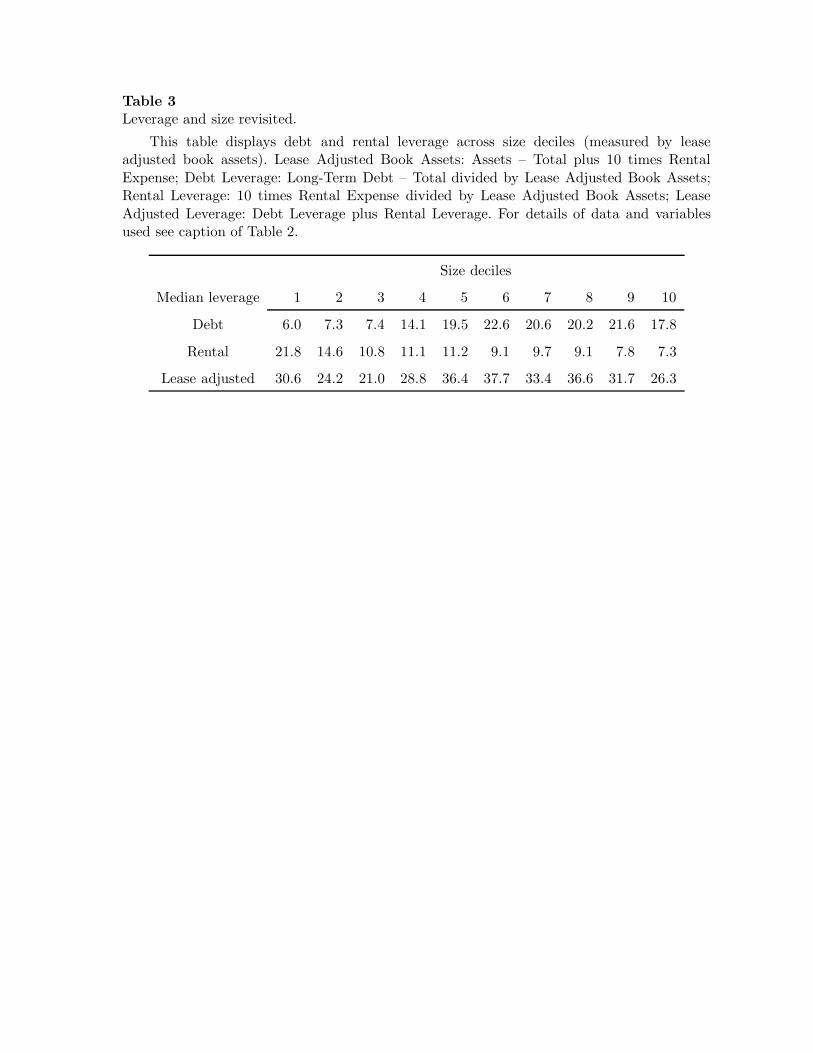
Table 3
Leverage and size revisited.
This table displays debt and rental leverage across size deciles (measured by leaseadjusted book assets). Lease Adjusted Book Assets: Assets – Total plus 10 times Rental
Expense; Debt Leverage: Long-Term Debt – Total divided by Lease Adjusted Book Assets;Rental Leverage: 10 times Rental Expense divided by Lease Adjusted Book Assets; Lease
Adjusted Leverage: Debt Leverage plus Rental Leverage. For details of data and variablesused see caption of Table 2.
Size deciles
Median leverage 1 2 3 4 5 6 7 8 9 10
Debt 6.0 7.3 7.4 14.1 19.5 22.6 20.6 20.2 21.6 17.8
Rental 21.8 14.6 10.8 11.1 11.2 9.1 9.7 9.1 7.8 7.3
Lease adjusted 30.6 24.2 21.0 28.8 36.4 37.7 33.4 36.6 31.7 26.3

1 2 3 4 5 6 7 8 9 100
5
10
15
20
25
30
35
40
(Lease adjusted) size deciles
Lease
adju
ste
d, debt, a
nd r
en
tal le
vera
ge (
%)
Fig. 1. Leverage versus size revisited. Lease adjusted leverage (solid), debt leverage (dashed),and rental leverage (dash dotted) across size decicles for Compustat firms. For details see
caption of Table 3.
0 0.2 0.4 0.60
0.2
0.4
0.6
A. Investment
Current net worth
0 0.2 0.4 0.60
0.02
0.04
0.06B. Risk management
Current net worth
0 0.2 0.4 0.60
0.2
0.4
0.6
C. Net worth next period
Current net worth
0 0.2 0.4 0.60
0.5
1D. Multipliers on collateral constraints
Current net worth
Fig. 2. Investment and risk management. Panel A shows investment k; Panel B shows riskmanagement for the low state h(s′1); Panel C shows net worth in low state next period w(s′1)
(solid) and in high state next period w(s′2) (dashed); Panel D shows scaled multipliers on thecollateral constraint for the low state next period βλ(s′1)/µ (solid) and for the high state nextperiod βλ(s′2)/µ (dashed); all as a function of current net worth w. The parameter values are:
β = 0.93, r = 0.05, δ = 0.10, m = +∞, θ = 0.80, ϕ = 1, A(s2) = 0.6, A(s1) = 0.05, andΠ(s, s′) = 0.5, ∀s, s′ ∈ S, and f(k) = kα with α = 0.333.
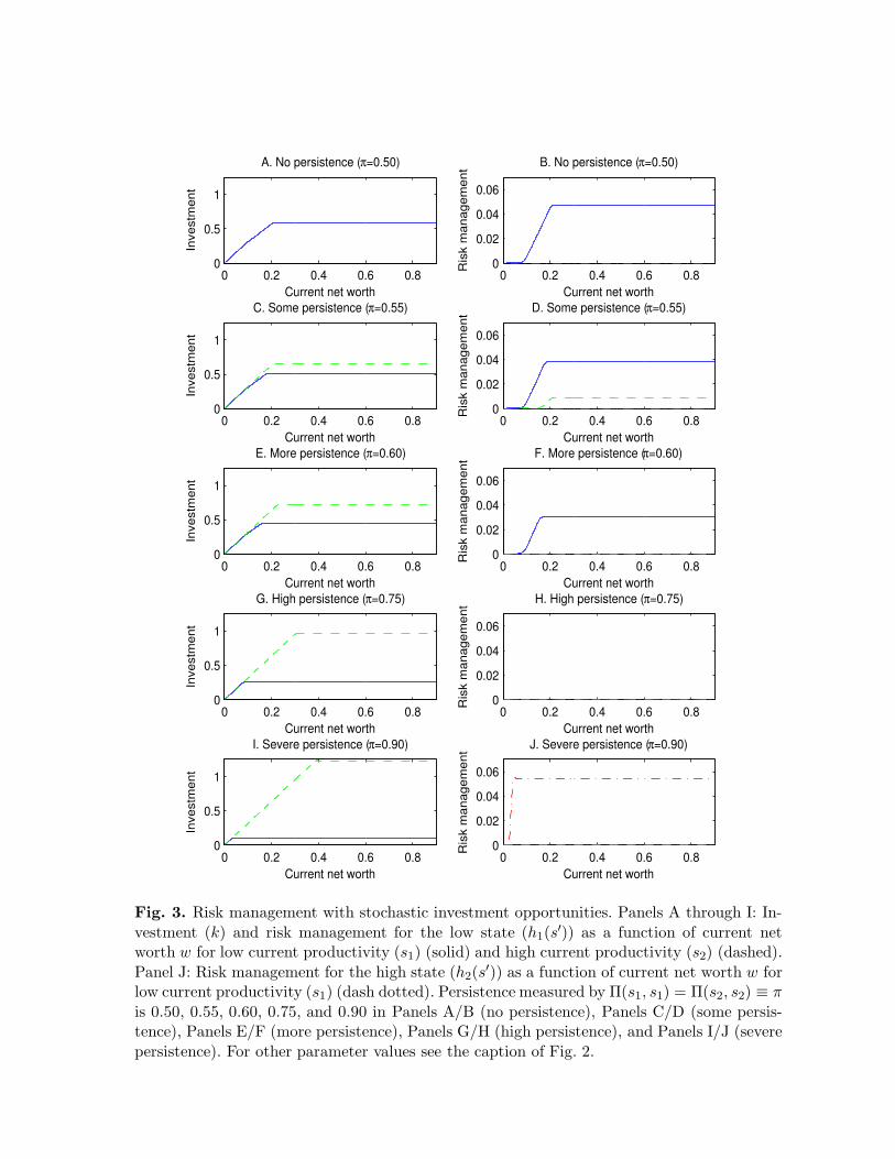
0 0.2 0.4 0.6 0.80
0.5
1
A. No persistence (π=0.50)
Inve
stm
en
t
Current net worth
0 0.2 0.4 0.6 0.80
0.02
0.04
0.06
B. No persistence (π=0.50)
Ris
k m
an
ag
em
en
t
Current net worth
0 0.2 0.4 0.6 0.80
0.5
1
C. Some persistence (π=0.55)
Inve
stm
en
t
Current net worth
0 0.2 0.4 0.6 0.80
0.02
0.04
0.06
D. Some persistence (π=0.55)
Ris
k m
an
ag
em
en
t
Current net worth
0 0.2 0.4 0.6 0.80
0.5
1
E. More persistence (π=0.60)
Inve
stm
en
t
Current net worth
0 0.2 0.4 0.6 0.80
0.02
0.04
0.06
F. More persistence (π=0.60)R
isk m
an
ag
em
en
t
Current net worth
0 0.2 0.4 0.6 0.80
0.5
1
G. High persistence (π=0.75)
Inve
stm
en
t
Current net worth
0 0.2 0.4 0.6 0.80
0.02
0.04
0.06
H. High persistence (π=0.75)
Ris
k m
an
ag
em
en
t
Current net worth
0 0.2 0.4 0.6 0.80
0.5
1
I. Severe persistence (π=0.90)
Inve
stm
en
t
Current net worth
0 0.2 0.4 0.6 0.80
0.02
0.04
0.06
J. Severe persistence (π=0.90)
Ris
k m
an
ag
em
en
t
Current net worth
Fig. 3. Risk management with stochastic investment opportunities. Panels A through I: In-
vestment (k) and risk management for the low state (h1(s′)) as a function of current net
worth w for low current productivity (s1) (solid) and high current productivity (s2) (dashed).
Panel J: Risk management for the high state (h2(s′)) as a function of current net worth w for
low current productivity (s1) (dash dotted). Persistence measured by Π(s1, s1) = Π(s2, s2) ≡ π
is 0.50, 0.55, 0.60, 0.75, and 0.90 in Panels A/B (no persistence), Panels C/D (some persis-tence), Panels E/F (more persistence), Panels G/H (high persistence), and Panels I/J (severe
persistence). For other parameter values see the caption of Fig. 2.

0 0.2 0.4 0.60
0.1
0.2
0.3
0.4
0.5
0.6
0.7A. Investment
Current net worth
0 0.2 0.4 0.60
0.01
0.02
0.03
0.04
0.05
0.06
0.07
0.08
0.09B. Risk management
Current net worth
Fig. 4. Investment and risk management: Effect of risk. Panel A shows investment k andPanel B shows risk management for the low state h(s′1) as a function of current net worth
w as risk varies. The parameter values are as in Fig. 2 except that (A(s2), A(s1)) vary from(0.625, 0.025) (dashed), (0.600, 0.050) (solid), (0.575, 0.075) (dash dotted), to (0.550, 0.100)(dotted).
0 0.2 0.4 0.60
0.1
0.2
0.3
0.4
0.5
0.6
0.7A. Investment
Current net worth
0 0.2 0.4 0.60
0.01
0.02
0.03
0.04
0.05
0.06
0.07B. Risk management
Current net worth
Fig. 5. Investment and risk management: Effect of tangibility and collateralizability. Panel Ashows investment k and Panel B shows risk management for the low state h(s′1) as a function
of current net worth w as tangibility or collateralizability varies. The parameter values are asin Fig. 2 except that θ varies from 0.9 (dashed), 0.8 (solid), 0.7 (dash dotted), to 0.6 (dotted).
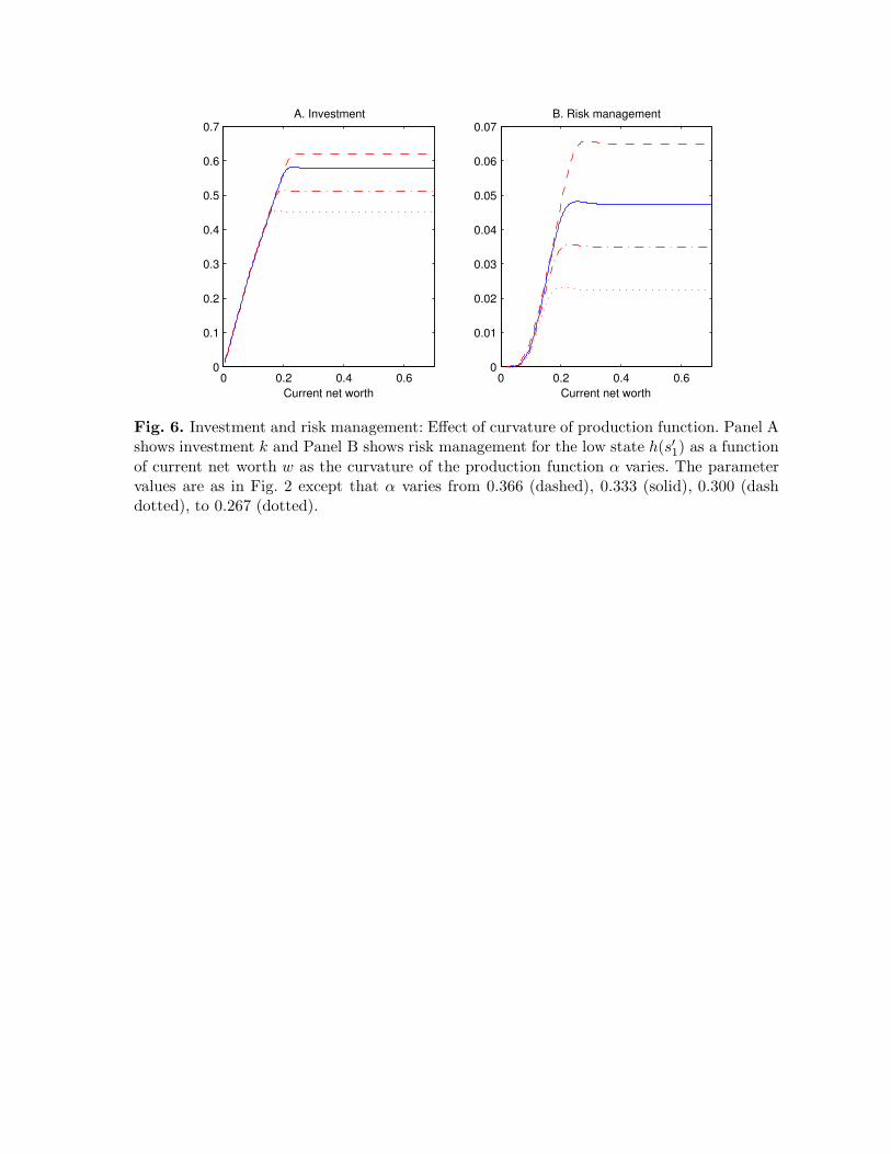
0 0.2 0.4 0.60
0.1
0.2
0.3
0.4
0.5
0.6
0.7A. Investment
Current net worth
0 0.2 0.4 0.60
0.01
0.02
0.03
0.04
0.05
0.06
0.07B. Risk management
Current net worth
Fig. 6. Investment and risk management: Effect of curvature of production function. Panel Ashows investment k and Panel B shows risk management for the low state h(s′1) as a function
of current net worth w as the curvature of the production function α varies. The parametervalues are as in Fig. 2 except that α varies from 0.366 (dashed), 0.333 (solid), 0.300 (dashdotted), to 0.267 (dotted).

0 0.2 0.4 0.60
0.2
0.4
0.6
A. Investment and leasing
Investm
ent and leasin
g
Current net worth
0 0.2 0.4 0.60
0.02
0.04
0.06B. Risk management
Ris
k m
anagem
ent
Current net worth
0 0.2 0.4 0.60
0.2
0.4
0.6
C. Net worth next period
Net w
ort
h n
ext period
Current net worth
0 0.2 0.4 0.60
0.5
1D. Multipliers on collateral constraints
Multip
liers
Current net worth
0 0.2 0.4 0.60
0.5
1E. Total, debt, and rental leverage
Levera
ge
Current net worth
Fig. 7. Leasing, leverage, and risk management. Panel A shows investment (k) (solid) andleasing (kl) (dashed); Panel B shows risk management for the low state (h1(s
′)); Panel C shows
net worth next period in the low state next period (w(s′1)) (solid) and in the high state nextperiod (w(s′2)) (dashed); Panel D shows the multipliers on the collateral constraints for the
low state (βλ(s′1)) (solid) and for the high state (βλ(s′2)) (dashed); and Panel E shows totalleverage (θ(ϕk − kl) + kl)/k (solid), debt leverage θ(ϕk − kl)/k (dashed), and rental leverage
kl/k (dash dotted); all as a function of current net worth w. For other parameter values seethe caption of Fig. 2 except that m = 0.01 and ϕ = 0.8.