Colin Wilson Department of Cognitive Science Johns · PDF file1 / 38 Bayesian inference for...
83
1 / 38 Bayesian inference for constraint-based phonology Colin Wilson Department of Cognitive Science Johns Hopkins University University of Massachusetts, Amherst December 2, 2011
-
Upload
vuongthuan -
Category
Documents
-
view
217 -
download
0
Transcript of Colin Wilson Department of Cognitive Science Johns · PDF file1 / 38 Bayesian inference for...
1 / 38
Bayesian inference for constraint-based phonology
Colin WilsonDepartment of Cognitive Science
Johns Hopkins University
University of Massachusetts, Amherst
December 2, 2011

Outline
2 / 38
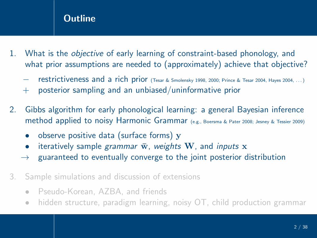
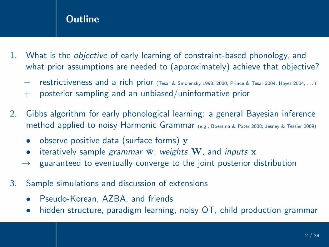
1. What is the objective of early learning of constraint-based phonology, andwhat prior assumptions are needed to (approximately) achieve that objective?
− restrictiveness and a rich prior (Tesar & Smolensky 1998, 2000; Prince & Tesar 2004, Hayes 2004, . . . )
+ posterior sampling and an unbiased/uninformative prior
2. Gibbs algorithm for early phonological learning: a general Bayesian inferencemethod applied to noisy Harmonic Grammar (e.g., Boersma & Pater 2008; Jesney & Tessier 2009)
• observe positive data (surface forms) y• iteratively sample grammar w, weights W, and inputs x
→ guaranteed to eventually converge to the joint posterior distribution
3. Sample simulations and discussion of extensions
• Pseudo-Korean, AZBA, and friends• hidden structure, paradigm learning, noisy OT, child production grammar
Outline
2 / 38
1. What is the objective of early learning of constraint-based phonology, andwhat prior assumptions are needed to (approximately) achieve that objective?
− restrictiveness and a rich prior (Tesar & Smolensky 1998, 2000; Prince & Tesar 2004, Hayes 2004, . . . )
+ posterior sampling and an unbiased/uninformative prior
2. Gibbs algorithm for early phonological learning: a general Bayesian inferencemethod applied to noisy Harmonic Grammar (e.g., Boersma & Pater 2008; Jesney & Tessier 2009)
• observe positive data (surface forms) y• iteratively sample grammar w, weights W, and inputs x
→ guaranteed to eventually converge to the joint posterior distribution
3. Sample simulations and discussion of extensions
• Pseudo-Korean, AZBA, and friends• hidden structure, paradigm learning, noisy OT, child production grammar
Early phonological learning
3 / 38
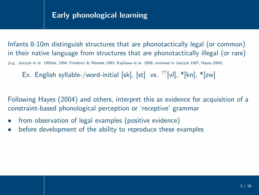
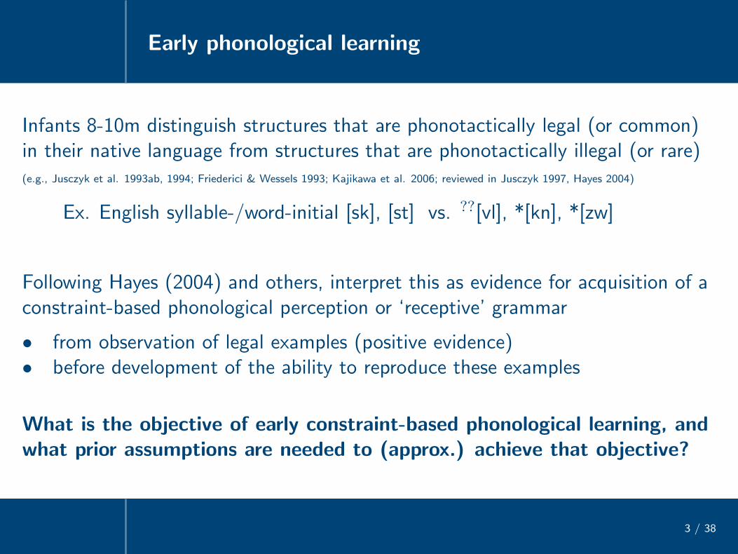
Infants 8-10m distinguish structures that are phonotactically legal (or common)in their native language from structures that are phonotactically illegal (or rare)(e.g., Jusczyk et al. 1993ab, 1994; Friederici & Wessels 1993; Kajikawa et al. 2006; reviewed in Jusczyk 1997, Hayes 2004)
Ex. English syllable-/word-initial [sk], [st] vs. ??[vl], *[kn], *[zw]
Following Hayes (2004) and others, interpret this as evidence for acquisition of aconstraint-based phonological perception or ‘receptive’ grammar
• from observation of legal examples (positive evidence)• before development of the ability to reproduce these examples
Early phonological learning
3 / 38
Infants 8-10m distinguish structures that are phonotactically legal (or common)in their native language from structures that are phonotactically illegal (or rare)(e.g., Jusczyk et al. 1993ab, 1994; Friederici & Wessels 1993; Kajikawa et al. 2006; reviewed in Jusczyk 1997, Hayes 2004)
Ex. English syllable-/word-initial [sk], [st] vs. ??[vl], *[kn], *[zw]
Following Hayes (2004) and others, interpret this as evidence for acquisition of aconstraint-based phonological perception or ‘receptive’ grammar
• from observation of legal examples (positive evidence)• before development of the ability to reproduce these examples
What is the objective of early constraint-based phonological learning, andwhat prior assumptions are needed to (approx.) achieve that objective?

The restrictiveness objective
4 / 38
Tesar & Smolensky (1998, 2000), Hayes (2004), Prince & Tesar (2004) and muchsubsequent work take the objective of learning to be grammar restrictiveness(see also earlier work on the subset problem, e.g., Baker 1979; Angluin 1980; Pinker 1986, and the associated subset principle, e.g.,
Berwick 1982, 1986; Jacubowitz 1984, Wexler & Manzini 1987)
For the learning of phonotactic distributions . . . the goal is always toselect the most restrictive grammar consistent with the data. Thecomputational challenge is efficiently to determine, for any given set ofdata, which grammar is the most restrictive. (Prince & Tesar 2004:249)
If the [learned] rankings are correct, the grammar will act as a filter:it will alter any illegal form to something similar which is legal, but itwill allow legal forms to persist unaltered. (Hayes 2004:168)
Running example: Pseudo-Korean (Hayes 2004)
5 / 38
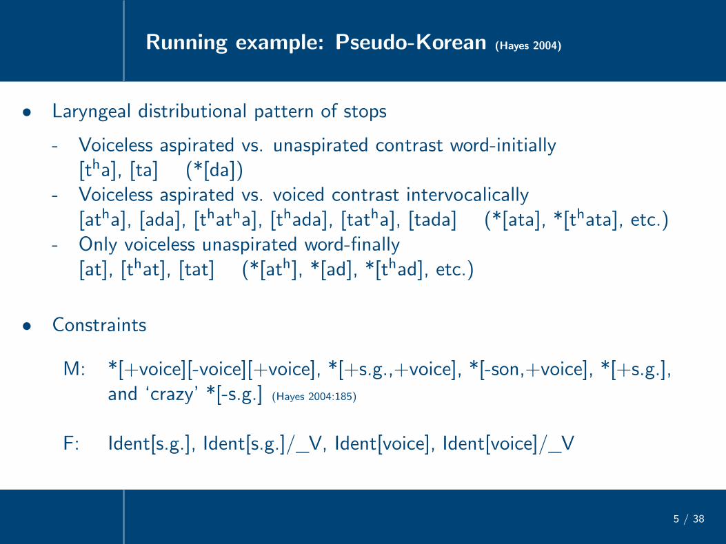
• Laryngeal distributional pattern of stops
- Voiceless aspirated vs. unaspirated contrast word-initially[tha], [ta] (*[da])
- Voiceless aspirated vs. voiced contrast intervocalically[atha], [ada], [thatha], [thada], [tatha], [tada] (*[ata], *[thata], etc.)
- Only voiceless unaspirated word-finally[at], [that], [tat] (*[ath], *[ad], *[thad], etc.)
• Constraints
M: *[+voice][-voice][+voice], *[+s.g.,+voice], *[-son,+voice], *[+s.g.],and ‘crazy’ *[-s.g.] (Hayes 2004:185)
F: Ident[s.g.], Ident[s.g.]/ V, Ident[voice], Ident[voice]/ V

Difficulty of achieving restrictiveness
6 / 38
In principle:
Multiple grammars can be consistent with the same data, grammarswhich are empirically distinct in that they make different predictionsabout other forms not represented in the data. If learning is basedupon only positive evidence, then the simple consistency of agrammatical hypothesis with all the observed data will not guaranteethat this hypothesis is correct . . . . (Prince & Tesar 2004:245)
In practice:
• Hayes (2004) ran the Recursive Constraint Demotion algorithm of Tesar(1995), Tesar & Smolensky (1998, 2000) on Pseduo-Korean and other cases
• The resulting grammars were quite unrestrictive: all IO-Faithfulnessconstraints in the top stratum, failing to ‘filter’ many types of illegal form
Toward restrictive learning: prior assumptions
7 / 38
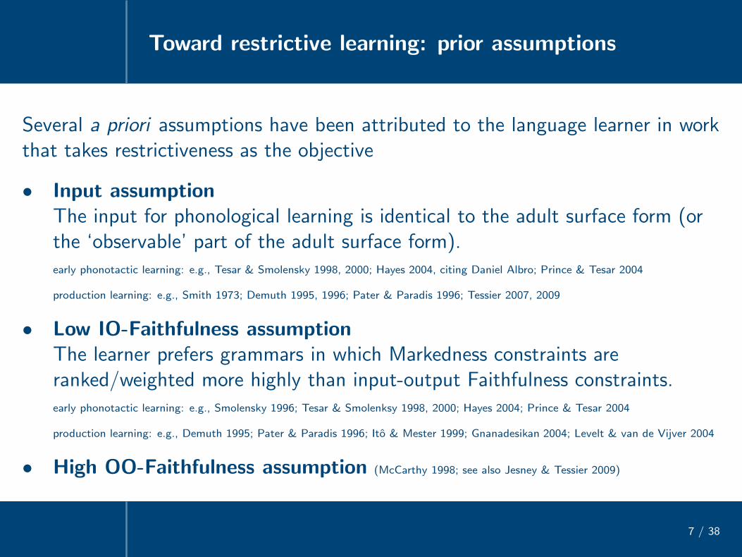
Several a priori assumptions have been attributed to the language learner in workthat takes restrictiveness as the objective
• Input assumptionThe input for phonological learning is identical to the adult surface form (orthe ‘observable’ part of the adult surface form).early phonotactic learning: e.g., Tesar & Smolensky 1998, 2000; Hayes 2004, citing Daniel Albro; Prince & Tesar 2004
production learning: e.g., Smith 1973; Demuth 1995, 1996; Pater & Paradis 1996; Tessier 2007, 2009
• Low IO-Faithfulness assumptionThe learner prefers grammars in which Markedness constraints areranked/weighted more highly than input-output Faithfulness constraints.early phonotactic learning: e.g., Smolensky 1996; Tesar & Smolenksy 1998, 2000; Hayes 2004; Prince & Tesar 2004
production learning: e.g., Demuth 1995; Pater & Paradis 1996; Ito & Mester 1999; Gnanadesikan 2004; Levelt & van de Vijver 2004
• High OO-Faithfulness assumption (McCarthy 1998; see also Jesney & Tessier 2009)
Toward restrictive learning: mechanisms
8 / 38
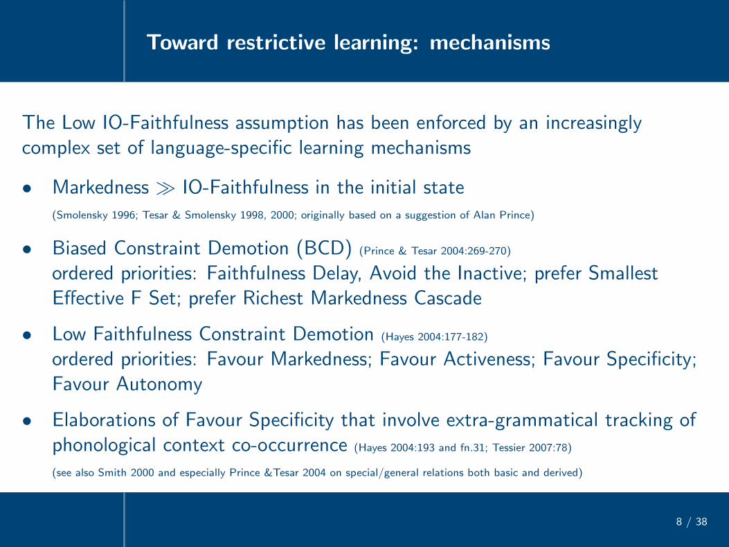
The Low IO-Faithfulness assumption has been enforced by an increasinglycomplex set of language-specific learning mechanisms
• Markedness ≫ IO-Faithfulness in the initial state(Smolensky 1996; Tesar & Smolensky 1998, 2000; originally based on a suggestion of Alan Prince)
• Biased Constraint Demotion (BCD) (Prince & Tesar 2004:269-270)
ordered priorities: Faithfulness Delay, Avoid the Inactive; prefer SmallestEffective F Set; prefer Richest Markedness Cascade
• Low Faithfulness Constraint Demotion (Hayes 2004:177-182)
ordered priorities: Favour Markedness; Favour Activeness; Favour Specificity;Favour Autonomy
• Elaborations of Favour Specificity that involve extra-grammatical tracking ofphonological context co-occurrence (Hayes 2004:193 and fn.31; Tessier 2007:78)
(see also Smith 2000 and especially Prince &Tesar 2004 on special/general relations both basic and derived)
Review of learning with the restrictiveness objective
9 / 38
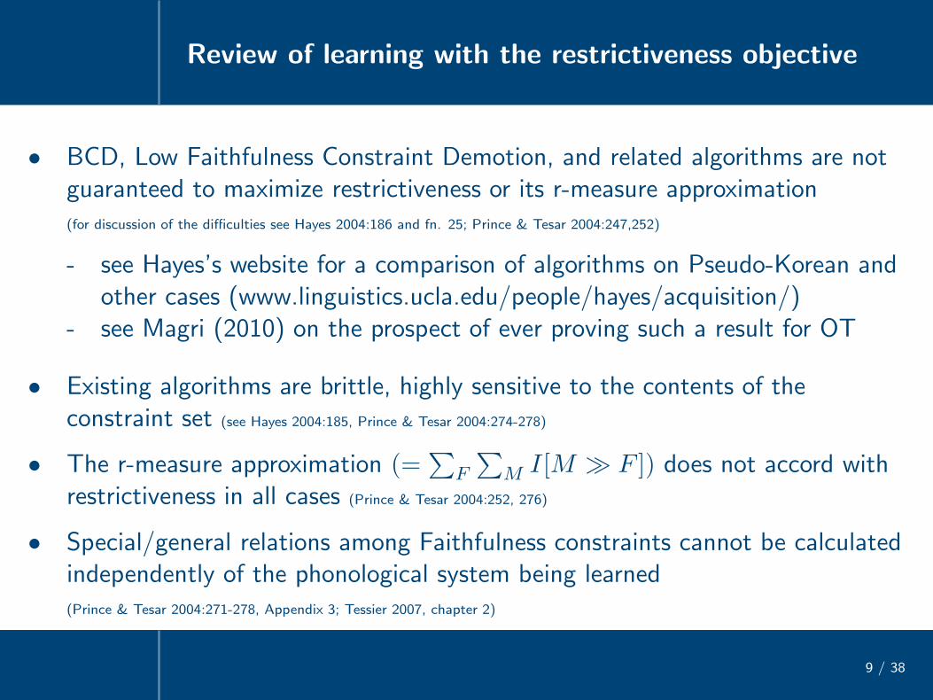
• BCD, Low Faithfulness Constraint Demotion, and related algorithms are notguaranteed to maximize restrictiveness or its r-measure approximation(for discussion of the difficulties see Hayes 2004:186 and fn. 25; Prince & Tesar 2004:247,252)
- see Hayes’s website for a comparison of algorithms on Pseudo-Korean andother cases (www.linguistics.ucla.edu/people/hayes/acquisition/)
- see Magri (2010) on the prospect of ever proving such a result for OT
• Existing algorithms are brittle, highly sensitive to the contents of theconstraint set (see Hayes 2004:185, Prince & Tesar 2004:274-278)
• The r-measure approximation (=∑
F
∑
M I[M ≫ F ]) does not accord withrestrictiveness in all cases (Prince & Tesar 2004:252, 276)
• Special/general relations among Faithfulness constraints cannot be calculatedindependently of the phonological system being learned(Prince & Tesar 2004:271-278, Appendix 3; Tessier 2007, chapter 2)

Where to go from here?
10 / 38
• Switch from OT to HG can perhaps simplify the set of a priori learningassumptions (e.g., Jesney & Tessier 2009), but still no general guaranteesabout the restrictiveness of the learned grammars
• Jarosz (2006, 2007) proposes to change the learner’s objective — this talkbuilds on Jarosz’s work within a more general Bayesian framework, and with avery different type of inference algorithm

Where to go from here?
11 / 38
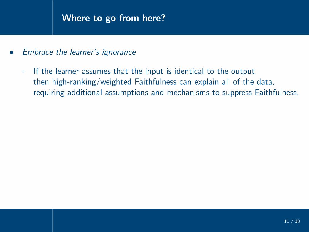
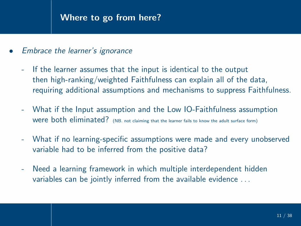
• Embrace the learner’s ignorance
Where to go from here?
11 / 38
• Embrace the learner’s ignorance
- If the learner assumes that the input is identical to the outputthen high-ranking/weighted Faithfulness can explain all of the data,requiring additional assumptions and mechanisms to suppress Faithfulness.
Where to go from here?
11 / 38
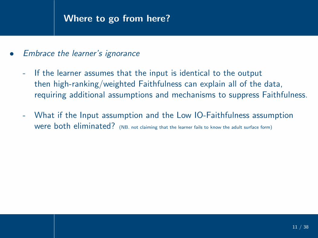
• Embrace the learner’s ignorance
- If the learner assumes that the input is identical to the outputthen high-ranking/weighted Faithfulness can explain all of the data,requiring additional assumptions and mechanisms to suppress Faithfulness.
- What if the Input assumption and the Low IO-Faithfulness assumptionwere both eliminated? (NB. not claiming that the learner fails to know the adult surface form)
Where to go from here?
11 / 38
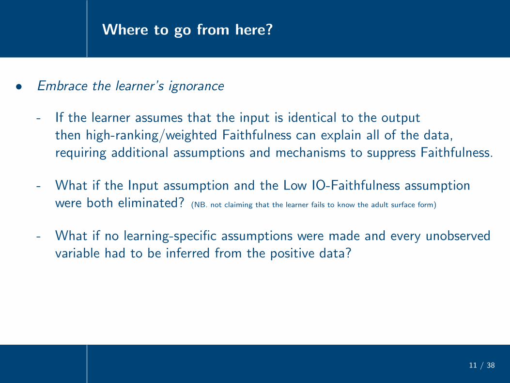
• Embrace the learner’s ignorance
- If the learner assumes that the input is identical to the outputthen high-ranking/weighted Faithfulness can explain all of the data,requiring additional assumptions and mechanisms to suppress Faithfulness.
- What if the Input assumption and the Low IO-Faithfulness assumptionwere both eliminated? (NB. not claiming that the learner fails to know the adult surface form)
- What if no learning-specific assumptions were made and every unobservedvariable had to be inferred from the positive data?
Where to go from here?
11 / 38
• Embrace the learner’s ignorance
- If the learner assumes that the input is identical to the outputthen high-ranking/weighted Faithfulness can explain all of the data,requiring additional assumptions and mechanisms to suppress Faithfulness.
- What if the Input assumption and the Low IO-Faithfulness assumptionwere both eliminated? (NB. not claiming that the learner fails to know the adult surface form)
- What if no learning-specific assumptions were made and every unobservedvariable had to be inferred from the positive data?
- Need a learning framework in which multiple interdependent hiddenvariables can be jointly inferred from the available evidence . . .
Bayesian inference for constraint-based
phonology with Gibbs sampling
12 / 38
Bayesian grammatical inference
13 / 38
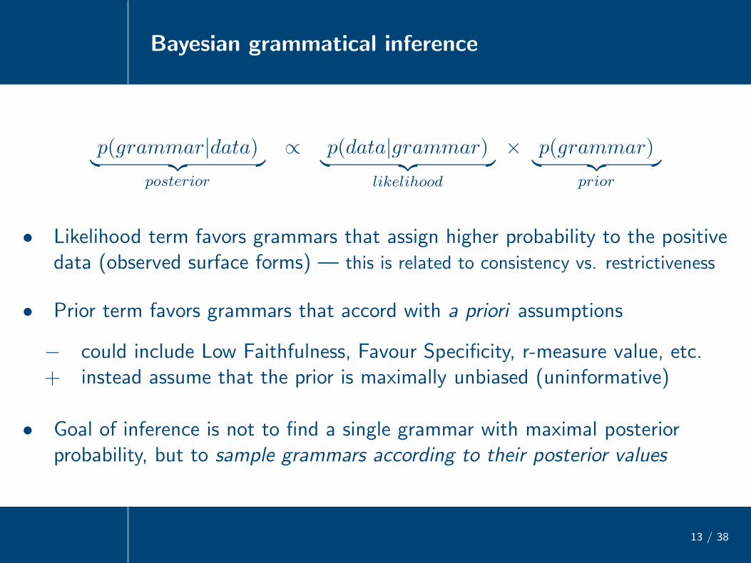
p(grammar|data)︸ ︷︷ ︸
posterior
∝ p(data|grammar)︸ ︷︷ ︸
likelihood
× p(grammar)︸ ︷︷ ︸
prior
• Likelihood term favors grammars that assign higher probability to the positivedata (observed surface forms) — this is related to consistency vs. restrictiveness
• Prior term favors grammars that accord with a priori assumptions
− could include Low Faithfulness, Favour Specificity, r-measure value, etc.+ instead assume that the prior is maximally unbiased (uninformative)
• Goal of inference is not to find a single grammar with maximal posteriorprobability, but to sample grammars according to their posterior values
Specialization to noisy Harmonic Grammar
14 / 38
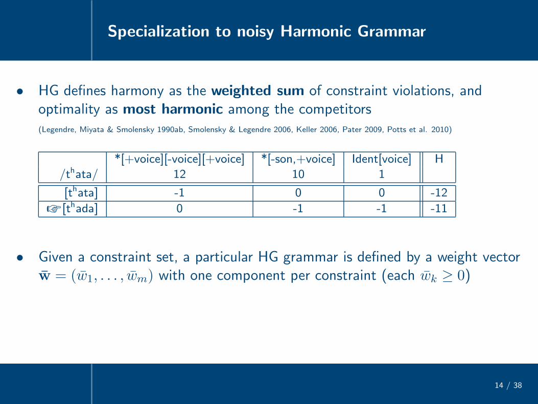
• HG defines harmony as the weighted sum of constraint violations, andoptimality as most harmonic among the competitors(Legendre, Miyata & Smolensky 1990ab, Smolensky & Legendre 2006, Keller 2006, Pater 2009, Potts et al. 2010)
*[+voice][-voice][+voice] *[-son,+voice] Ident[voice] H
/thata/ 12 10 1
[thata] -1 0 0 -12
☞ [thada] 0 -1 -1 -11
• Given a constraint set, a particular HG grammar is defined by a weight vectorw = (w1, . . . , wm) with one component per constraint (each wk ≥ 0)
Specialization to noisy Harmonic Grammar
14 / 38
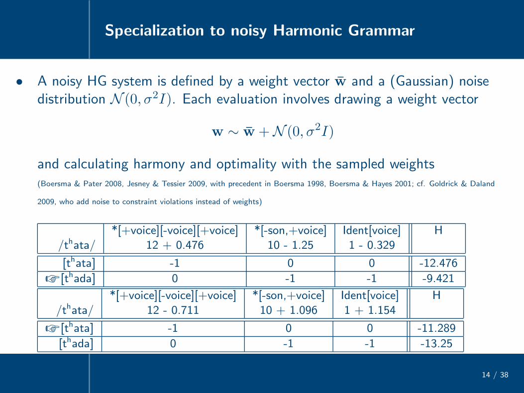
• A noisy HG system is defined by a weight vector w and a (Gaussian) noisedistribution N (0, σ2I). Each evaluation involves drawing a weight vector
w ∼ w +N (0, σ2I)
and calculating harmony and optimality with the sampled weights(Boersma & Pater 2008, Jesney & Tessier 2009, with precedent in Boersma 1998, Boersma & Hayes 2001; cf. Goldrick & Daland
2009, who add noise to constraint violations instead of weights)
*[+voice][-voice][+voice] *[-son,+voice] Ident[voice] H/thata/ 12 + 0.476 10 - 1.25 1 - 0.329
[thata] -1 0 0 -12.476
☞ [thada] 0 -1 -1 -9.421
*[+voice][-voice][+voice] *[-son,+voice] Ident[voice] H
/thata/ 12 - 0.711 10 + 1.096 1 + 1.154
☞ [thata] -1 0 0 -11.289
[thada] 0 -1 -1 -13.25
Specialization to noisy Harmonic Grammar
14 / 38
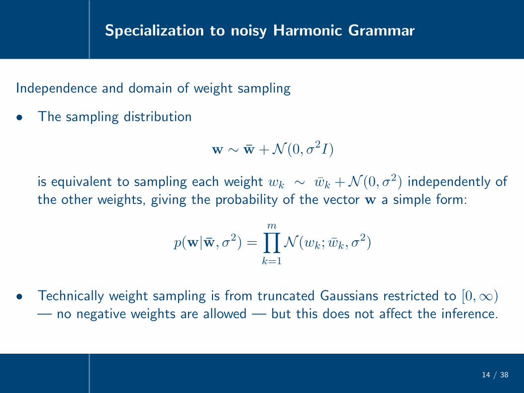
Independence and domain of weight sampling
• The sampling distribution
w ∼ w +N (0, σ2I)
is equivalent to sampling each weight wk ∼ wk +N (0, σ2) independently ofthe other weights, giving the probability of the vector w a simple form:
p(w|w, σ2) =m∏
k=1
N (wk; wk, σ2)
• Technically weight sampling is from truncated Gaussians restricted to [0,∞)— no negative weights are allowed — but this does not affect the inference.
Notation
15 / 38
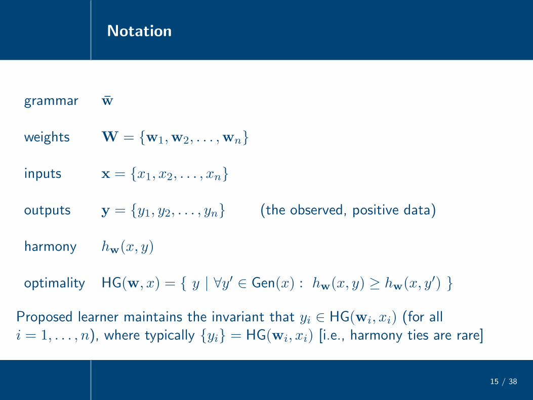
grammar w
weights W = {w1,w2, . . . ,wn}
inputs x = {x1, x2, . . . , xn}
outputs y = {y1, y2, . . . , yn} (the observed, positive data)
harmony hw(x, y)
optimality HG(w, x) = { y | ∀y′ ∈ Gen(x) : hw(x, y) ≥ hw(x, y′) }
Proposed learner maintains the invariant that yi ∈ HG(wi, xi) (for alli = 1, . . . , n), where typically {yi} = HG(wi, xi) [i.e., harmony ties are rare]
Graphical model of the data
16 / 38
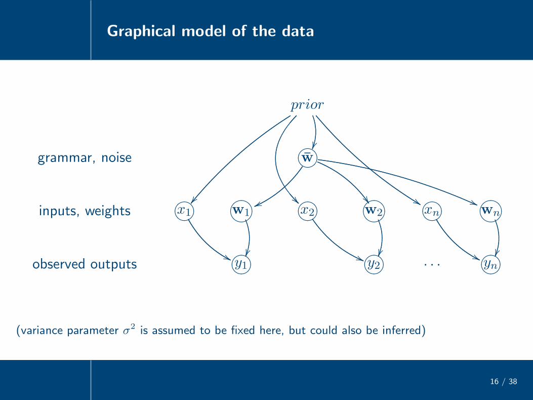
prior
�� �� %%
grammar, noise 76540123w
vv �� ((
inputs, weights 76540123x1
''
?>=<89:;w1
76540123x2
((
?>=<89:;w2
76540123xn
''
?>=<89:;wn
observed outputs 76540123y1 76540123y2 . . . 76540123yn
(variance parameter σ2 is assumed to be fixed here, but could also be inferred)

The inference problem
17 / 38
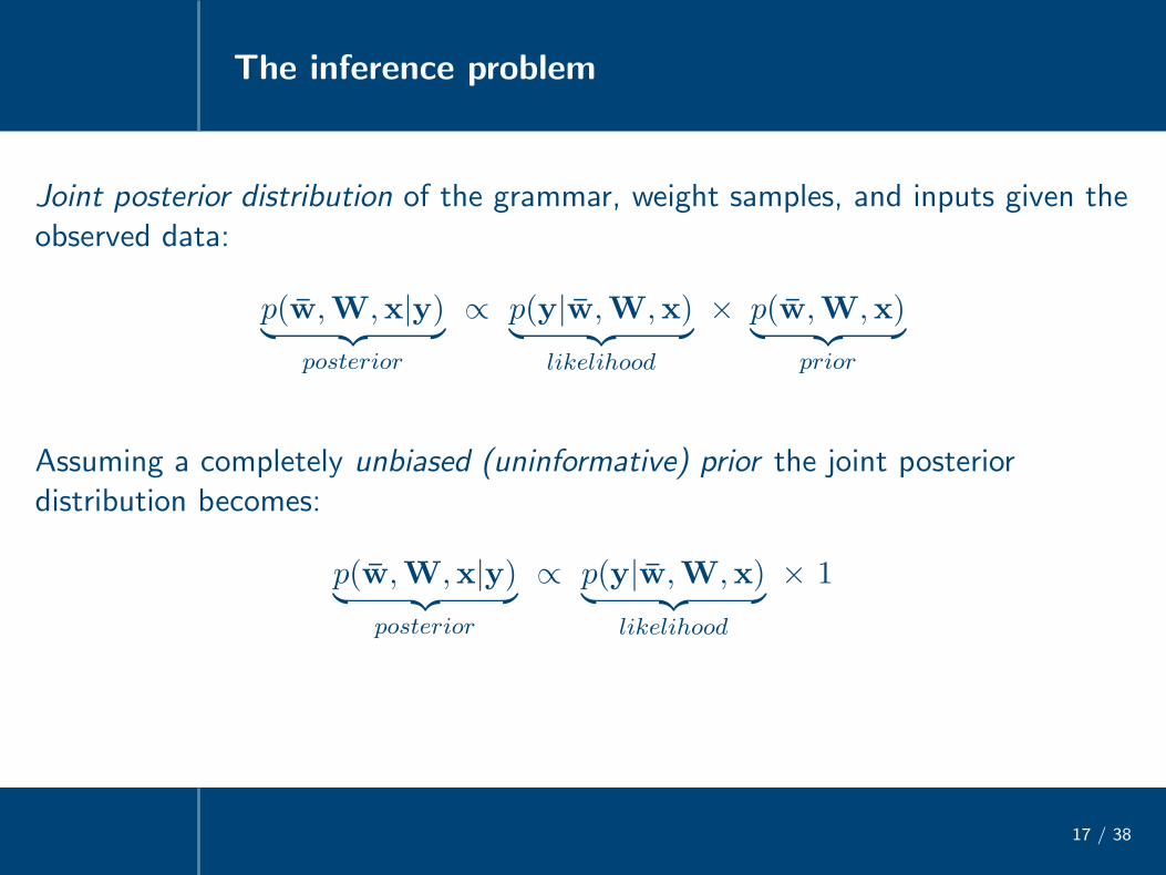
Joint posterior distribution of the grammar, weight samples, and inputs given theobserved data:
p(w,W,x|y)︸ ︷︷ ︸
posterior
∝ p(y|w,W,x)︸ ︷︷ ︸
likelihood
× p(w,W,x)︸ ︷︷ ︸
prior
The inference problem
17 / 38
Joint posterior distribution of the grammar, weight samples, and inputs given theobserved data:
p(w,W,x|y)︸ ︷︷ ︸
posterior
∝ p(y|w,W,x)︸ ︷︷ ︸
likelihood
× p(w,W,x)︸ ︷︷ ︸
prior
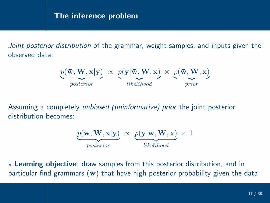
Assuming a completely unbiased (uninformative) prior the joint posteriordistribution becomes:
p(w,W,x|y)︸ ︷︷ ︸
posterior
∝ p(y|w,W,x)︸ ︷︷ ︸
likelihood
× 1
The inference problem
17 / 38
Joint posterior distribution of the grammar, weight samples, and inputs given theobserved data:
p(w,W,x|y)︸ ︷︷ ︸
posterior
∝ p(y|w,W,x)︸ ︷︷ ︸
likelihood
× p(w,W,x)︸ ︷︷ ︸
prior
Assuming a completely unbiased (uninformative) prior the joint posteriordistribution becomes:
p(w,W,x|y)︸ ︷︷ ︸
posterior
∝ p(y|w,W,x)︸ ︷︷ ︸
likelihood
× 1
⋆ Learning objective: draw samples from this posterior distribution, and inparticular find grammars (w) that have high posterior probability given the data
Analyzing the inference problem
18 / 38
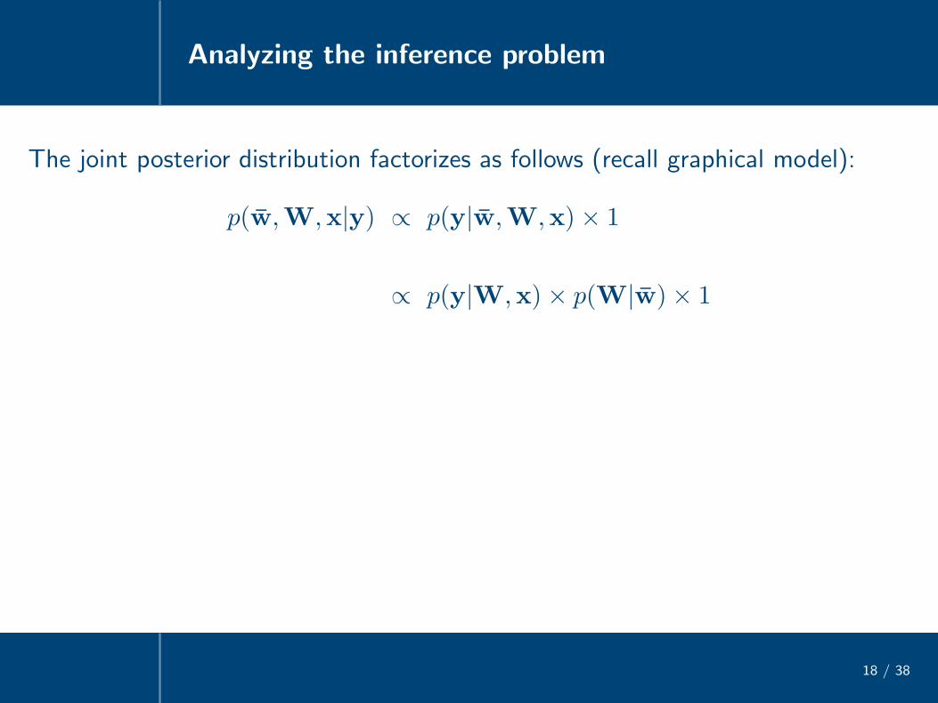
The joint posterior distribution factorizes as follows (recall graphical model):
p(w,W,x|y) ∝ p(y|w,W,x)× 1
∝ p(y|W,x)× p(W|w)× 1

Analyzing the inference problem
18 / 38
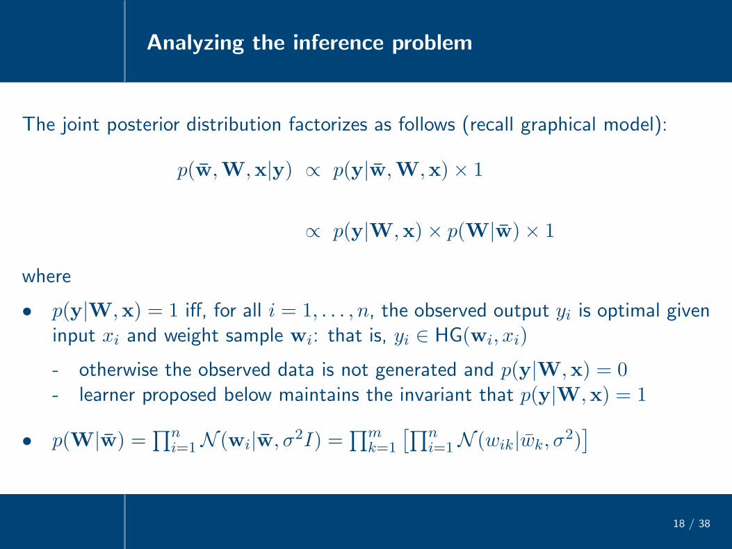
The joint posterior distribution factorizes as follows (recall graphical model):
p(w,W,x|y) ∝ p(y|w,W,x)× 1
∝ p(y|W,x)× p(W|w)× 1
where
• p(y|W,x) = 1 iff, for all i = 1, . . . , n, the observed output yi is optimal giveninput xi and weight sample wi: that is, yi ∈ HG(wi, xi)
- otherwise the observed data is not generated and p(y|W,x) = 0- learner proposed below maintains the invariant that p(y|W,x) = 1
Analyzing the inference problem
18 / 38
The joint posterior distribution factorizes as follows (recall graphical model):
p(w,W,x|y) ∝ p(y|w,W,x)× 1
∝ p(y|W,x)× p(W|w)× 1
where
• p(y|W,x) = 1 iff, for all i = 1, . . . , n, the observed output yi is optimal giveninput xi and weight sample wi: that is, yi ∈ HG(wi, xi)
- otherwise the observed data is not generated and p(y|W,x) = 0- learner proposed below maintains the invariant that p(y|W,x) = 1
• p(W|w) =∏n
i=1N (wi|w, σ2I) =∏m
k=1
[∏ni=1N (wik|wk, σ
2)]
Analyzing the inference problem
19 / 38
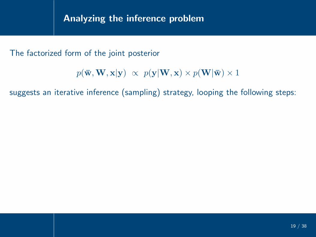
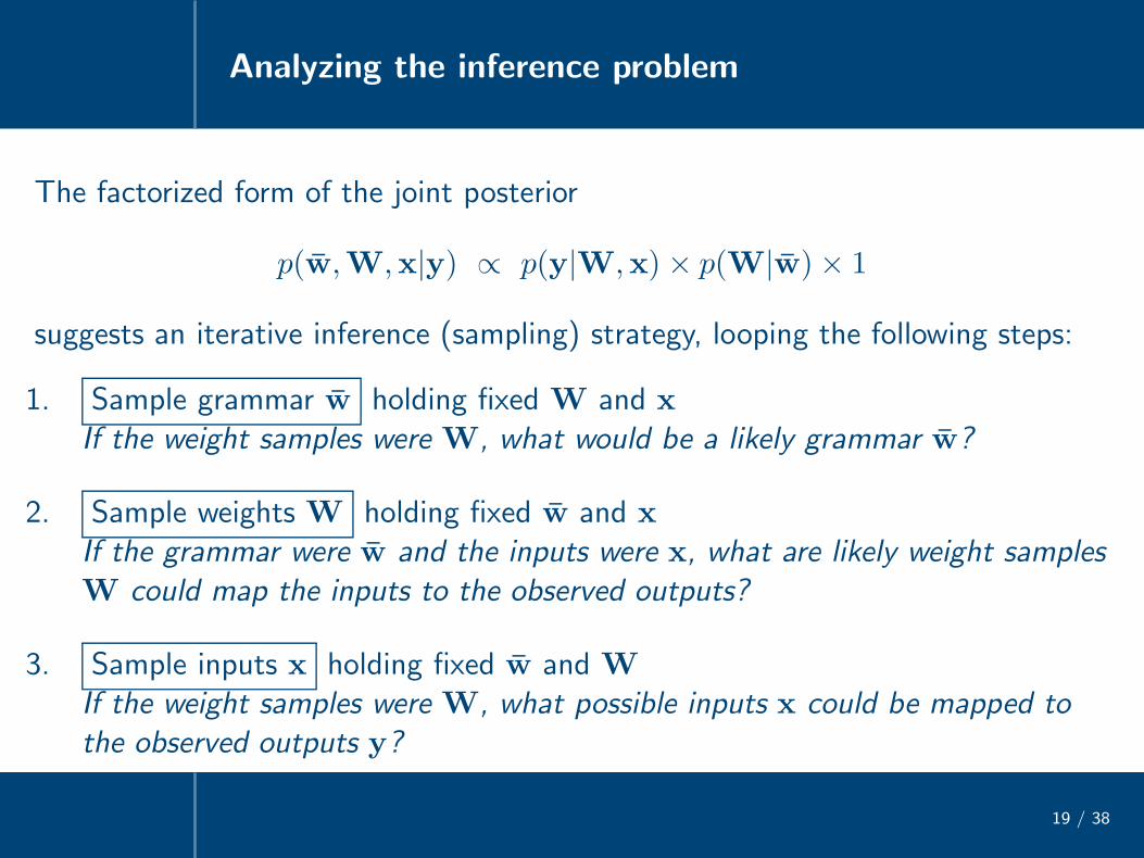
The factorized form of the joint posterior
p(w,W,x|y) ∝ p(y|W,x)× p(W|w)× 1
suggests an iterative inference (sampling) strategy, looping the following steps:

Analyzing the inference problem
19 / 38
The factorized form of the joint posterior
p(w,W,x|y) ∝ p(y|W,x)× p(W|w)× 1
suggests an iterative inference (sampling) strategy, looping the following steps:
1. Sample grammar w holding fixed W and x
If the weight samples were W, what would be a likely grammar w?
2. Sample weights W holding fixed w and x
If the grammar were w and the inputs were x, what are likely weight samplesW could map the inputs to the observed outputs?
3. Sample inputs x holding fixed w and W
If the weight samples were W, what possible inputs x could be mapped tothe observed outputs y?
Interim summary
20 / 38
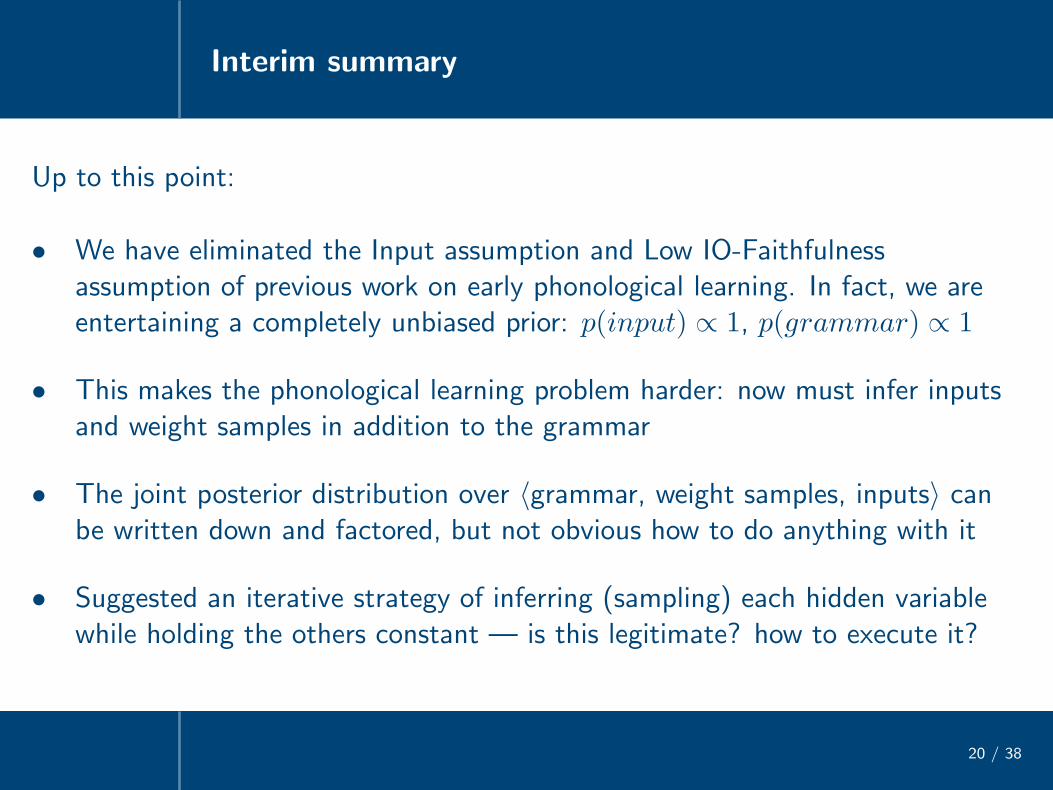
Up to this point:
• We have eliminated the Input assumption and Low IO-Faithfulnessassumption of previous work on early phonological learning. In fact, we areentertaining a completely unbiased prior: p(input) ∝ 1, p(grammar) ∝ 1
Interim summary
20 / 38
Up to this point:
• We have eliminated the Input assumption and Low IO-Faithfulnessassumption of previous work on early phonological learning. In fact, we areentertaining a completely unbiased prior: p(input) ∝ 1, p(grammar) ∝ 1
• This makes the phonological learning problem harder: now must infer inputsand weight samples in addition to the grammar
• The joint posterior distribution over 〈grammar, weight samples, inputs〉 canbe written down and factored, but not obvious how to do anything with it
• Suggested an iterative strategy of inferring (sampling) each hidden variablewhile holding the others constant — is this legitimate? how to execute it?
Gibbs sampling
21 / 38
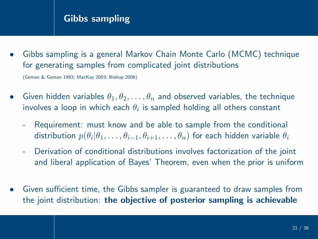
• Gibbs sampling is a general Markov Chain Monte Carlo (MCMC) techniquefor generating samples from complicated joint distributions(Geman & Geman 1993; MacKay 2003; Bishop 2006)
• Given hidden variables θ1, θ2, . . . , θn and observed variables, the techniqueinvolves a loop in which each θi is sampled holding all others constant
- Requirement: must know and be able to sample from the conditionaldistribution p(θi|θ1, . . . , θi−1, θi+1, . . . , θn) for each hidden variable θi
- Derivation of conditional distributions involves factorization of the jointand liberal application of Bayes’ Theorem, even when the prior is uniform
• Given sufficient time, the Gibbs sampler is guaranteed to draw samples fromthe joint distribution: the objective of posterior sampling is achievable

Gibbs sampling algorithm for noisy HG
22 / 38
Notation: α(t) is the value of variable α at discrete ‘time’ or step t, whereinitialization of all variables occurs at time t = 0
Initialization
• For each observed surface form yi, select an initial input x(0)i and a weight
sample w(0)i such that w
(0)i maps xi to yi: that is, yi ∈ HG(w
(0)i , x
(0)i )
- can initially set x(0)i := yi (recall the Input assumption)
- given (x(0)i , yi), can find w
(0)i using the simplex algorithm
(Dantzig 1981/1982, Chvatal 1983, Cormen et al. 2001; see Potts et al. 2010 on HG specifcially)
Gibbs sampling algorithm for noisy HG
22 / 38
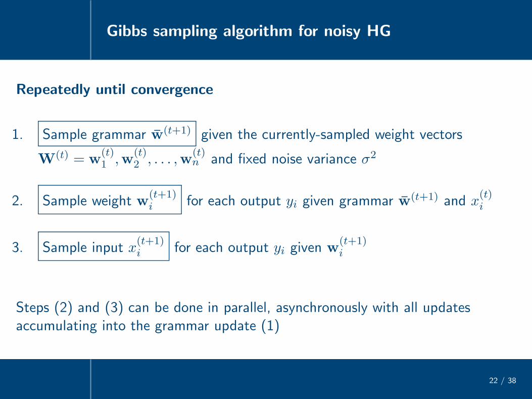
Repeatedly until convergence
1. Sample grammar w(t+1) given the currently-sampled weight vectors
W(t) = w(t)1 ,w
(t)2 , . . . ,w
(t)n and fixed noise variance σ2
2. Sample weight w(t+1)i for each output yi given grammar w(t+1) and x
(t)i
3. Sample input x(t+1)i for each output yi given w
(t+1)i
Steps (2) and (3) can be done in parallel, asynchronously with all updatesaccumulating into the grammar update (1)
Graphical model of the data (repeated)
23 / 38
prior
�� �� %%
grammar, noise 76540123w
vv �� ((
inputs, weights 76540123x1
''
?>=<89:;w1
76540123x2
((
?>=<89:;w2
76540123xn
''
?>=<89:;wn
observed outputs 76540123y1 76540123y2 . . . 76540123yn
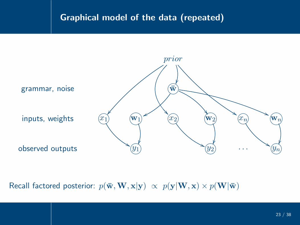
Recall factored posterior: p(w,W,x|y) ∝ p(y|W,x)× p(W|w)
1. Sampling a grammar
24 / 38
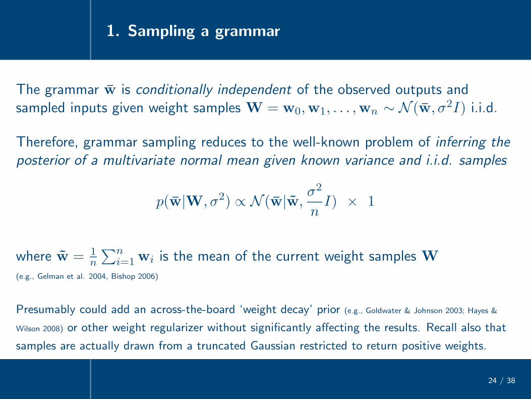
The grammar w is conditionally independent of the observed outputs andsampled inputs given weight samples W = w0,w1, . . . ,wn ∼ N (w, σ2I) i.i.d.
Therefore, grammar sampling reduces to the well-known problem of inferring theposterior of a multivariate normal mean given known variance and i.i.d. samples
p(w|W, σ2) ∝ N (w|w,σ2
nI) × 1
where w = 1n
∑ni=1wi is the mean of the current weight samples W
(e.g., Gelman et al. 2004, Bishop 2006)
Presumably could add an across-the-board ‘weight decay’ prior (e.g., Goldwater & Johnson 2003; Hayes &
Wilson 2008) or other weight regularizer without significantly affecting the results. Recall also that
samples are actually drawn from a truncated Gaussian restricted to return positive weights.
2. Sampling a weight vector
25 / 38
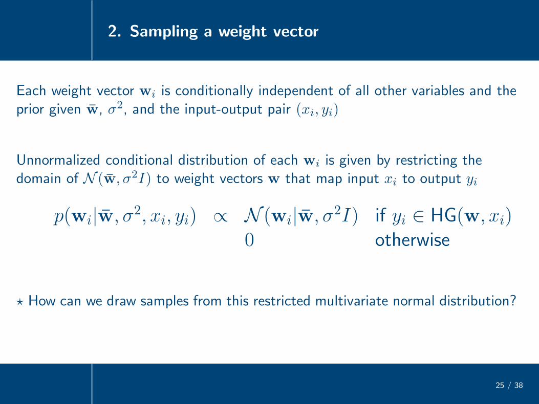
Each weight vector wi is conditionally independent of all other variables and theprior given w, σ2, and the input-output pair (xi, yi)
Unnormalized conditional distribution of each wi is given by restricting thedomain of N (w, σ2I) to weight vectors w that map input xi to output yi
p(wi|w, σ2, xi, yi) ∝ N (wi|w, σ2I) if yi ∈ HG(w, xi)0 otherwise
⋆ How can we draw samples from this restricted multivariate normal distribution?
2. Sampling a weight vector
25 / 38
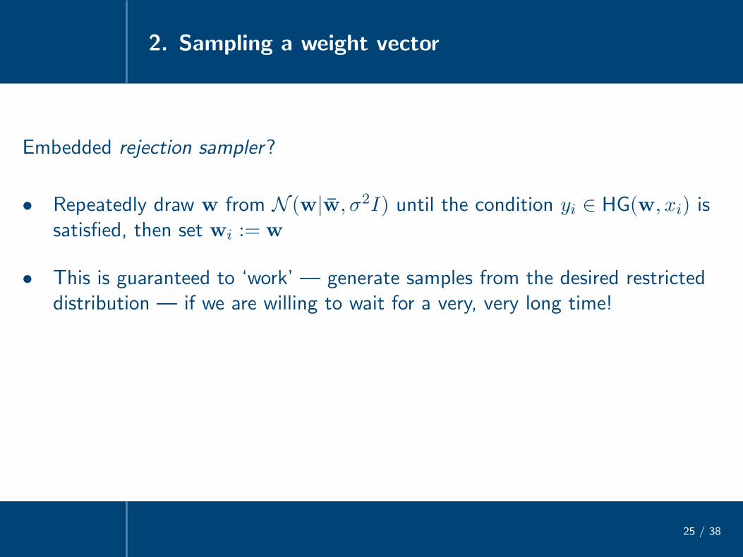
Embedded rejection sampler?
• Repeatedly draw w from N (w|w, σ2I) until the condition yi ∈ HG(w, xi) issatisfied, then set wi := w
• This is guaranteed to ‘work’ — generate samples from the desired restricteddistribution — if we are willing to wait for a very, very long time!
2. Sampling a weight vector
25 / 38
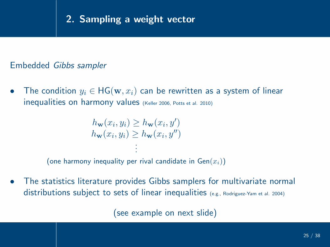
Embedded Gibbs sampler
• The condition yi ∈ HG(w, xi) can be rewritten as a system of linearinequalities on harmony values (Keller 2006, Potts et al. 2010)
hw(xi, yi) ≥ hw(xi, y′)
hw(xi, yi) ≥ hw(xi, y′′)
...(one harmony inequality per rival candidate in Gen(xi))
• The statistics literature provides Gibbs samplers for multivariate normaldistributions subject to sets of linear inequalities (e.g., Rodriguez-Yam et al. 2004)
(see example on next slide)
2. Sampling a weight vector
25 / 38
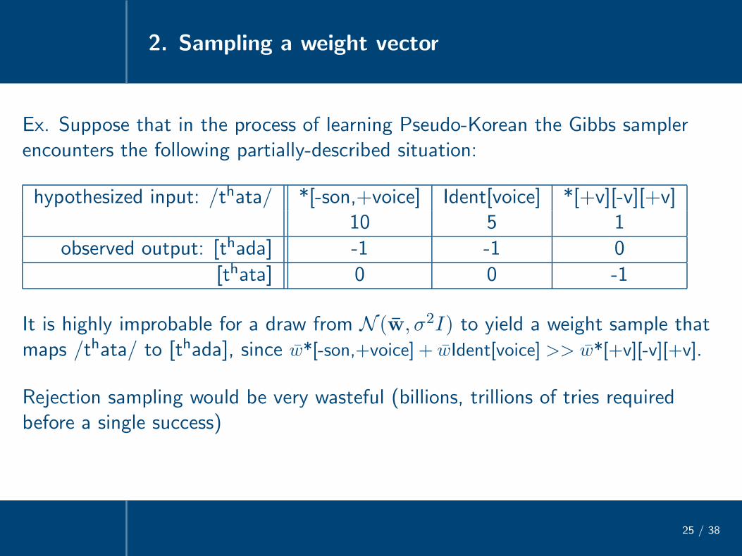
Ex. Suppose that in the process of learning Pseudo-Korean the Gibbs samplerencounters the following partially-described situation:
hypothesized input: /thata/ *[-son,+voice] Ident[voice] *[+v][-v][+v]10 5 1
observed output: [thada] -1 -1 0
[thata] 0 0 -1
It is highly improbable for a draw from N (w, σ2I) to yield a weight sample thatmaps /thata/ to [thada], since w*[-son,+voice]+ wIdent[voice] >> w*[+v][-v][+v].
Rejection sampling would be very wasteful (billions, trillions of tries requiredbefore a single success)
2. Sampling a weight vector
25 / 38
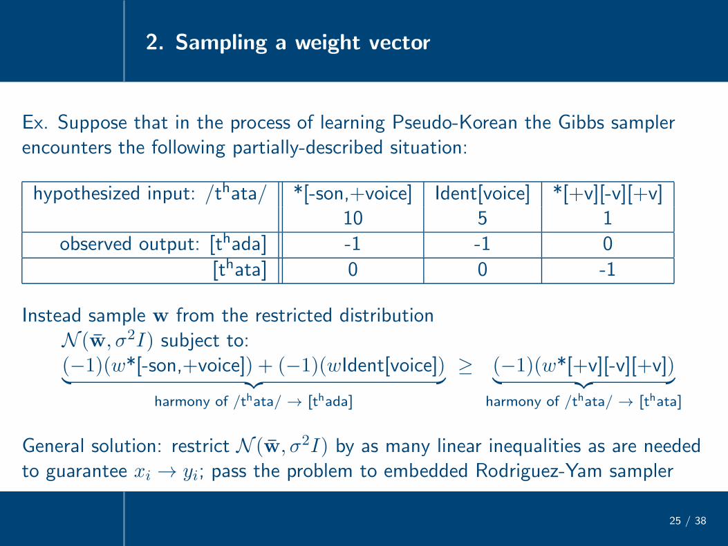
Ex. Suppose that in the process of learning Pseudo-Korean the Gibbs samplerencounters the following partially-described situation:
hypothesized input: /thata/ *[-son,+voice] Ident[voice] *[+v][-v][+v]10 5 1
observed output: [thada] -1 -1 0
[thata] 0 0 -1
Instead sample w from the restricted distributionN (w, σ2I) subject to:(−1)(w*[-son,+voice]) + (−1)(wIdent[voice])︸ ︷︷ ︸
harmony of /thata/ → [thada]
≥ (−1)(w*[+v][-v][+v])︸ ︷︷ ︸
harmony of /thata/ → [thata]
General solution: restrict N (w, σ2I) by as many linear inequalities as are neededto guarantee xi → yi; pass the problem to embedded Rodriguez-Yam sampler

3. Sampling an input
26 / 38
Each input xi is conditionally independent of all other random variables given theobserved output yi, the weight sample wi, and the prior
Conditional distribution of xi is given by restricting the space of all inputs tothose that are mapped to yi under the weighting wi (and normalizing)
p(xi|wi, yi) ∝ prior(xi) if yi ∈ HG(wi, xi)0 otherwise
What is the prior distribution over inputs? Assume uninformative, prior(x) ∝ 1,stochastic counterpart of Richness of the Base (see also Jarosz 2006, 2007)
⋆ How can we draw samples from this restricted distribution over inputs?

3. Sampling an input
26 / 38
Embedded rejection sampler?
• Repeatedly draw x from the rich base until the condition yi ∈ HG(wi, x) issatisfied, then set xi := x
• As before, this is guaranteed to eventually produce a sample from the desiredrestricted distribution eventually but can be extremely inefficient

3. Sampling an input
26 / 38
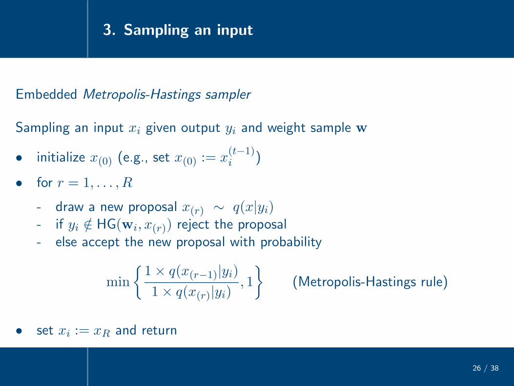
Embedded Metropolis-Hastings sampler
• The Input assumption of previous work asserted that the learner’s input isalways identical to the adult surface form
• A more flexible version of this assumption states that valid inputs are likely tolie ‘close’ to the observed output
• Provisional implementation
- Consider an observed output yi as the ‘center’ of a discrete string-editdistribution over potential inputs q(x|yi) (see for example Cortes et al. 2004, 2008 on the class
of rational kernels, Smith & Eisner 2005 on contrastive estimation)
- Potential inputs are proposed by q(x|yi) and accepted according to thestandard Metropolis-Hastings rule (Metropolis et al. 1953; Hastings 1970; MacKay 2003)
3. Sampling an input
26 / 38
Embedded Metropolis-Hastings sampler
Sampling an input xi given output yi and weight sample w
• initialize x(0) (e.g., set x(0) := x(t−1)i )
• for r = 1, . . . , R
- draw a new proposal x(r) ∼ q(x|yi)- if yi /∈ HG(wi, x(r)) reject the proposal- else accept the new proposal with probability
min
{1× q(x(r−1)|yi)
1× q(x(r)|yi), 1
}
(Metropolis-Hastings rule)
• set xi := xR and return
3. Sampling an input
26 / 38
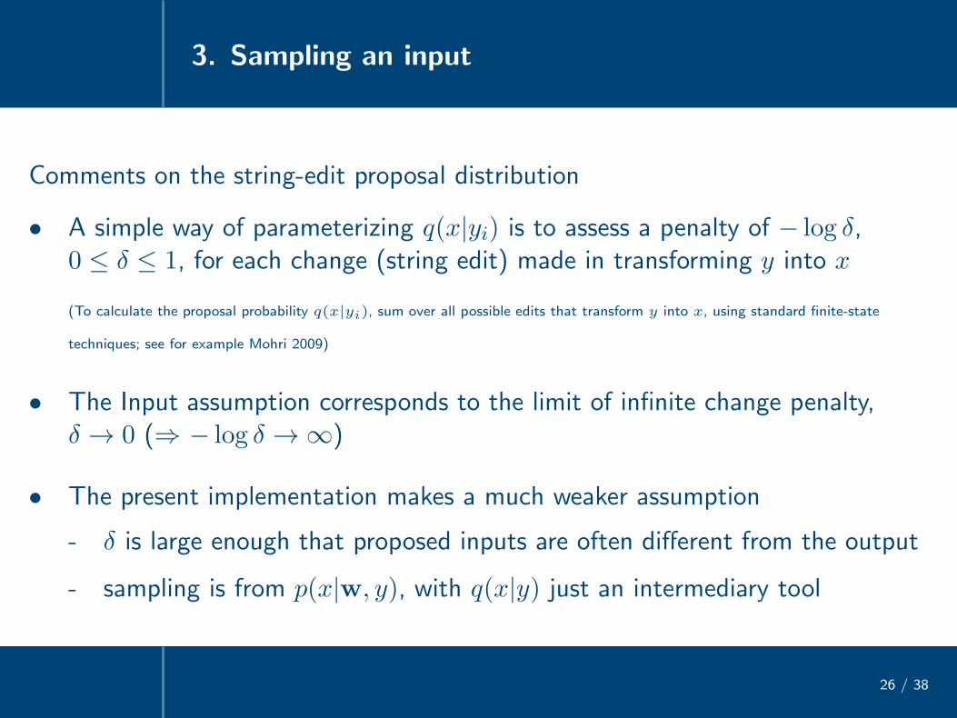
Comments on the string-edit proposal distribution
• A simple way of parameterizing q(x|yi) is to assess a penalty of − log δ,0 ≤ δ ≤ 1, for each change (string edit) made in transforming y into x
(To calculate the proposal probability q(x|yi), sum over all possible edits that transform y into x, using standard finite-state
techniques; see for example Mohri 2009)
• The Input assumption corresponds to the limit of infinite change penalty,δ → 0 (⇒ − log δ → ∞)
• The present implementation makes a much weaker assumption
- δ is large enough that proposed inputs are often different from the output
- sampling is from p(x|w, y), with q(x|y) just an intermediary tool
3. Sampling an input
26 / 38
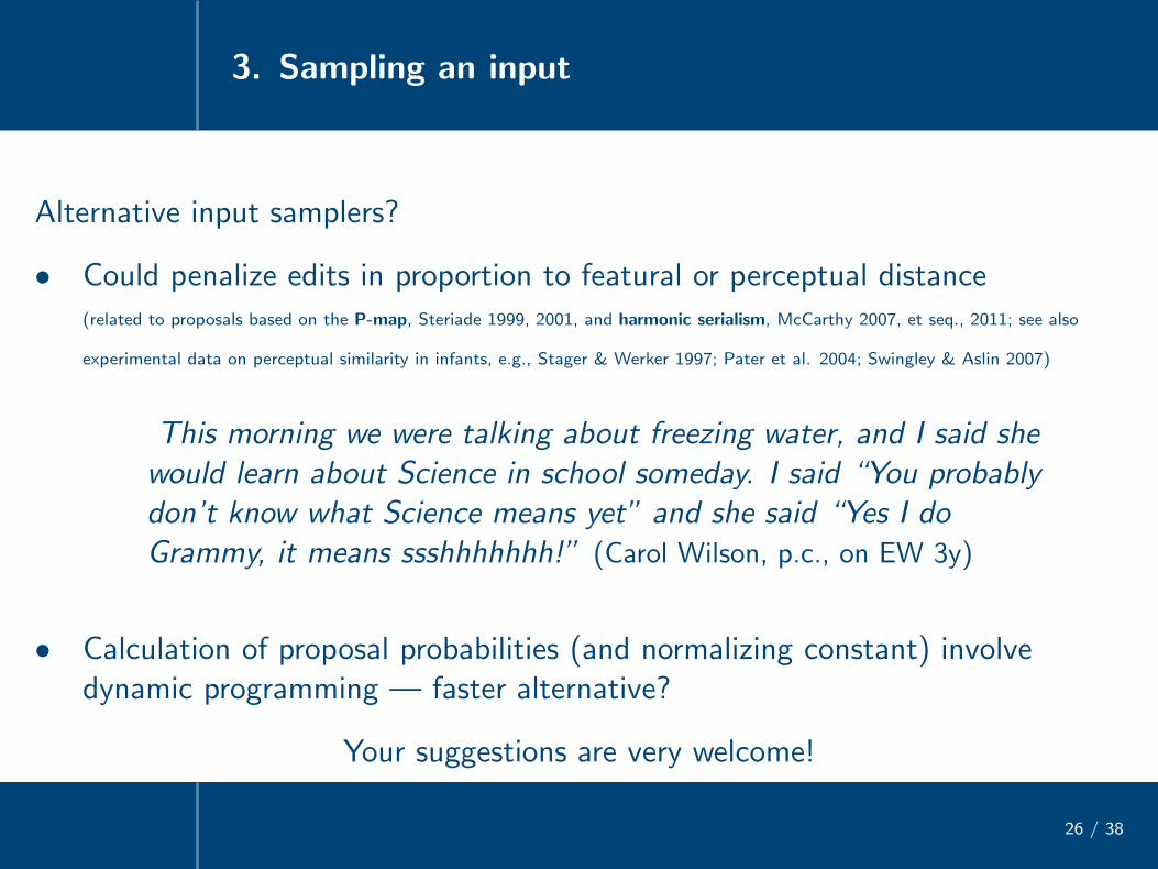
Alternative input samplers?
• Could penalize edits in proportion to featural or perceptual distance(related to proposals based on the P-map, Steriade 1999, 2001, and harmonic serialism, McCarthy 2007, et seq., 2011; see also
experimental data on perceptual similarity in infants, e.g., Stager & Werker 1997; Pater et al. 2004; Swingley & Aslin 2007)
This morning we were talking about freezing water, and I said shewould learn about Science in school someday. I said “You probablydon’t know what Science means yet” and she said “Yes I doGrammy, it means ssshhhhhhh!” (Carol Wilson, p.c., on EW 3y)
• Calculation of proposal probabilities (and normalizing constant) involvedynamic programming — faster alternative?
Your suggestions are very welcome!
Summary of Gibbs sampler
27 / 38
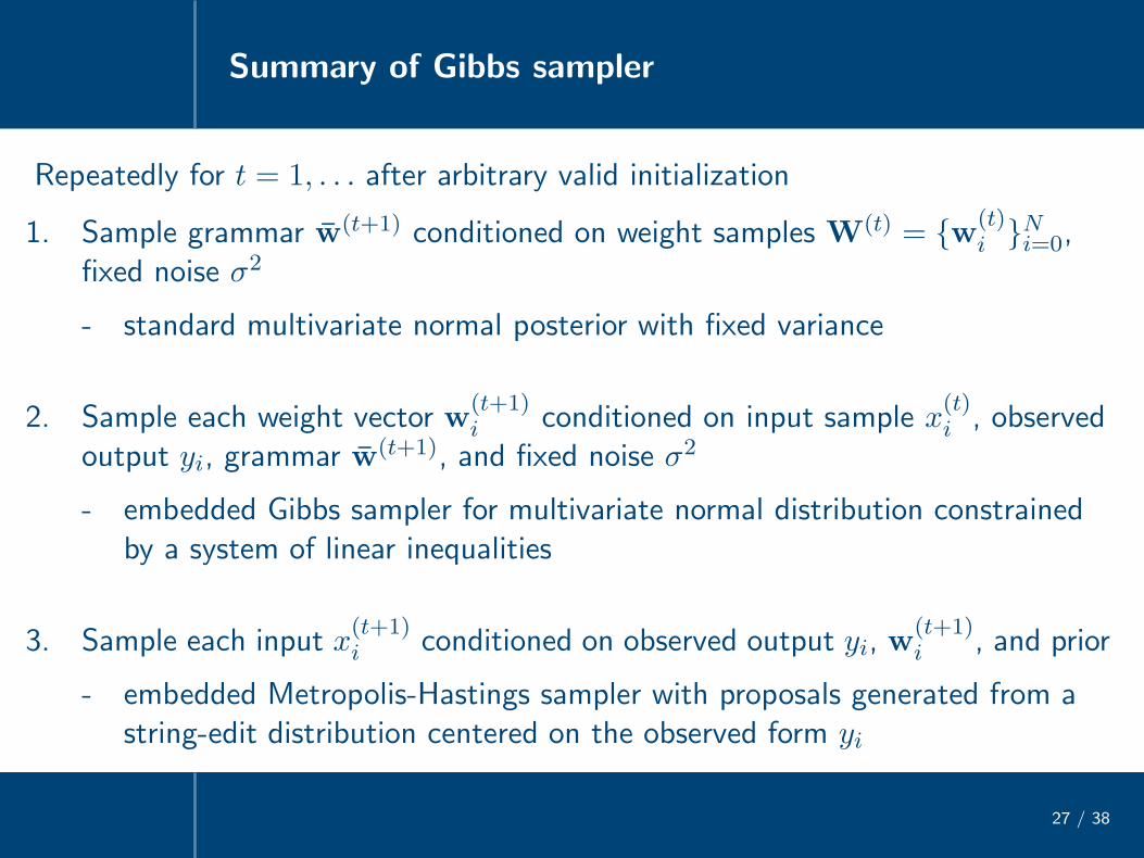
Repeatedly for t = 1, . . . after arbitrary valid initialization
1. Sample grammar w(t+1) conditioned on weight samples W(t) = {w(t)i }Ni=0,
fixed noise σ2
- standard multivariate normal posterior with fixed variance
2. Sample each weight vector w(t+1)i conditioned on input sample x
(t)i , observed
output yi, grammar w(t+1), and fixed noise σ2
- embedded Gibbs sampler for multivariate normal distribution constrainedby a system of linear inequalities
3. Sample each input x(t+1)i conditioned on observed output yi, w
(t+1)i , and prior
- embedded Metropolis-Hastings sampler with proposals generated from astring-edit distribution centered on the observed form yi
Products of the learner
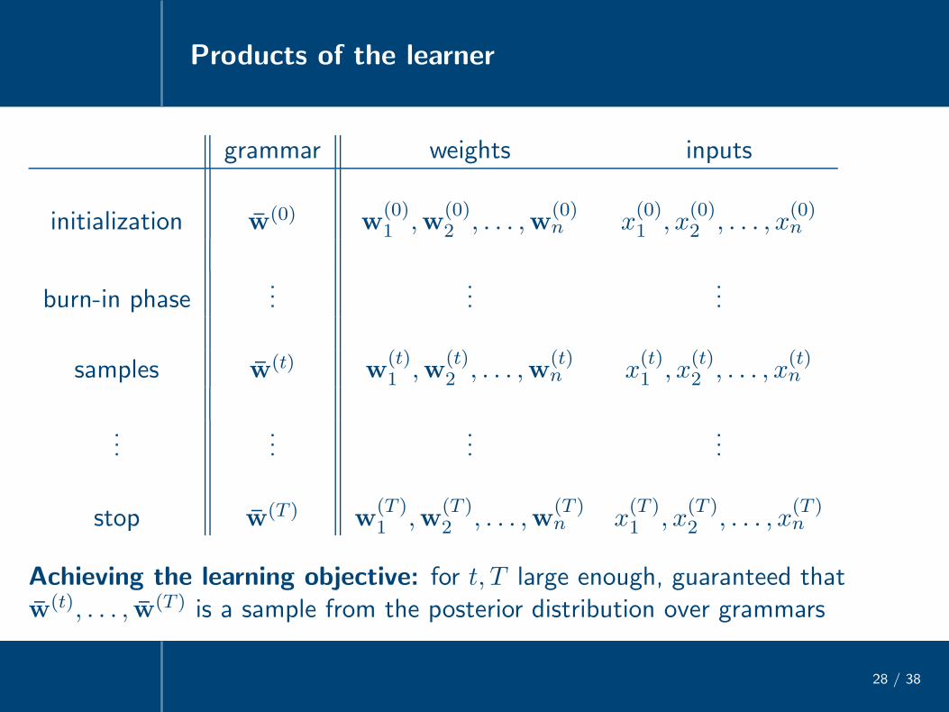
28 / 38
grammar weights inputs
initialization w(0) w(0)1 ,w
(0)2 , . . . ,w
(0)n x
(0)1 , x
(0)2 , . . . , x
(0)n
burn-in phase...
......
samples w(t) w(t)1 ,w
(t)2 , . . . ,w
(t)n x
(t)1 , x
(t)2 , . . . , x
(t)n
......
......
stop w(T ) w(T )1 ,w
(T )2 , . . . ,w
(T )n x
(T )1 , x
(T )2 , . . . , x
(T )n
Achieving the learning objective: for t, T large enough, guaranteed thatw(t), . . . , w(T ) is a sample from the posterior distribution over grammars
Examples, analysis, and extensions
29 / 38

Pseudo-Korean simulation
30 / 38
• Exhaustive set of inputs constructed from {th, t, d, dh, a} with skeletaCV, VC, CVC, CVCV
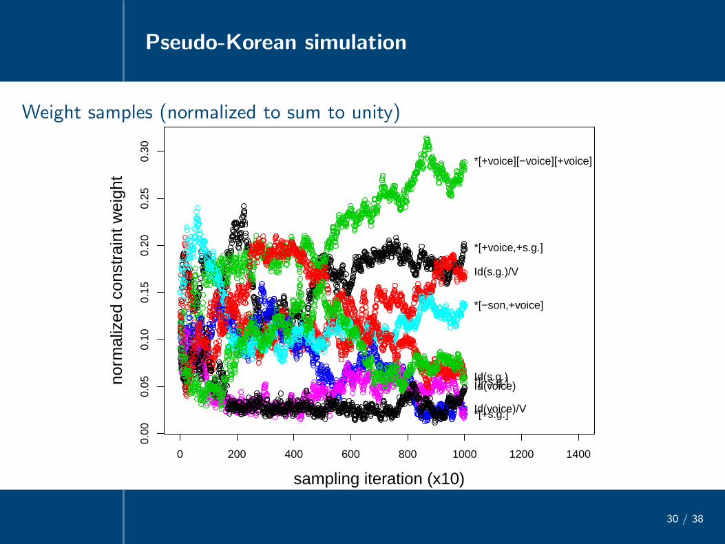
• Adult grammarM:*[+sg., +voice] 100F:Ident[s.g.]/ V 100M:*[+voice][-voice][+voice] 75M:*[+s.g.] 75M:*[-son,+voice] 50F:Ident[voice]/ V 1F:Ident[voice] 1F:Ident[s.g.] 1
• Adult language effectively deterministic with σ2 = 1
Pseudo-Korean simulation
30 / 38
Weight samples (normalized to sum to unity)
0 200 400 600 800 1000 1200 1400
0.00
0.05
0.10
0.15
0.20
0.25
0.30
sampling iteration (x10)
norm
aliz
ed c
onst
rain
t wei
ght
*[+voice,+s.g.]
Id(s.g.)/V
*[+voice][−voice][+voice]
*[+s.g.]
*[−son,+voice]
Id(voice)/V
Id(voice)Id(s.g.)*[−s.g.]
Pseudo-Korean simulation
30 / 38
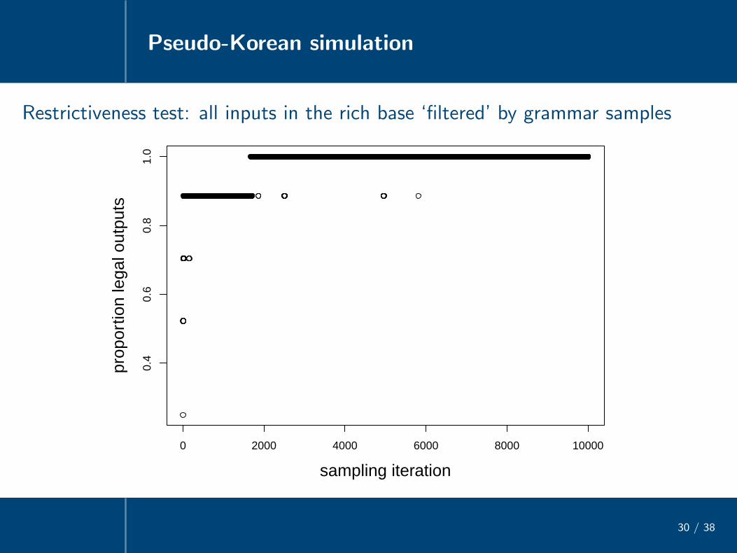
Restrictiveness test: all inputs in the rich base ‘filtered’ by grammar samples
0 2000 4000 6000 8000 10000
0.4
0.6
0.8
1.0
sampling iteration
prop
ortio
n le
gal o
utpu
ts
Pseudo-Korean simulation
30 / 38
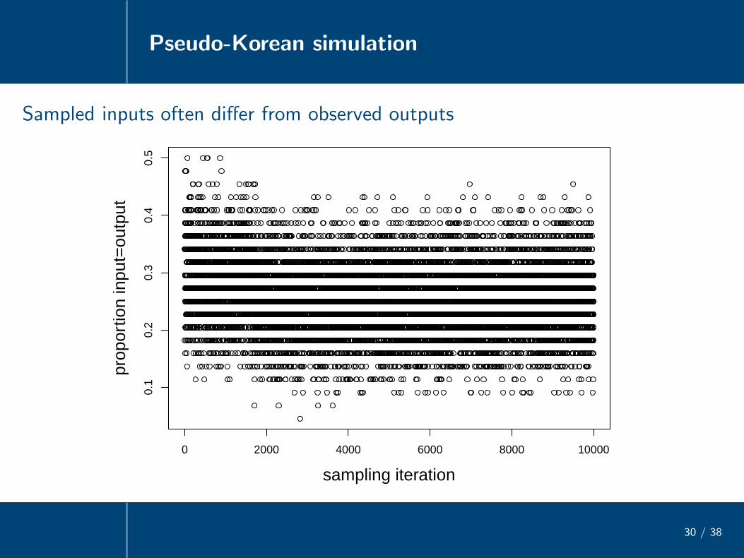
Sampled inputs often differ from observed outputs
0 2000 4000 6000 8000 10000
0.1
0.2
0.3
0.4
0.5
sampling iteration
prop
ortio
n in
put=
outp
ut
Pseudo-Korean simulation
30 / 38
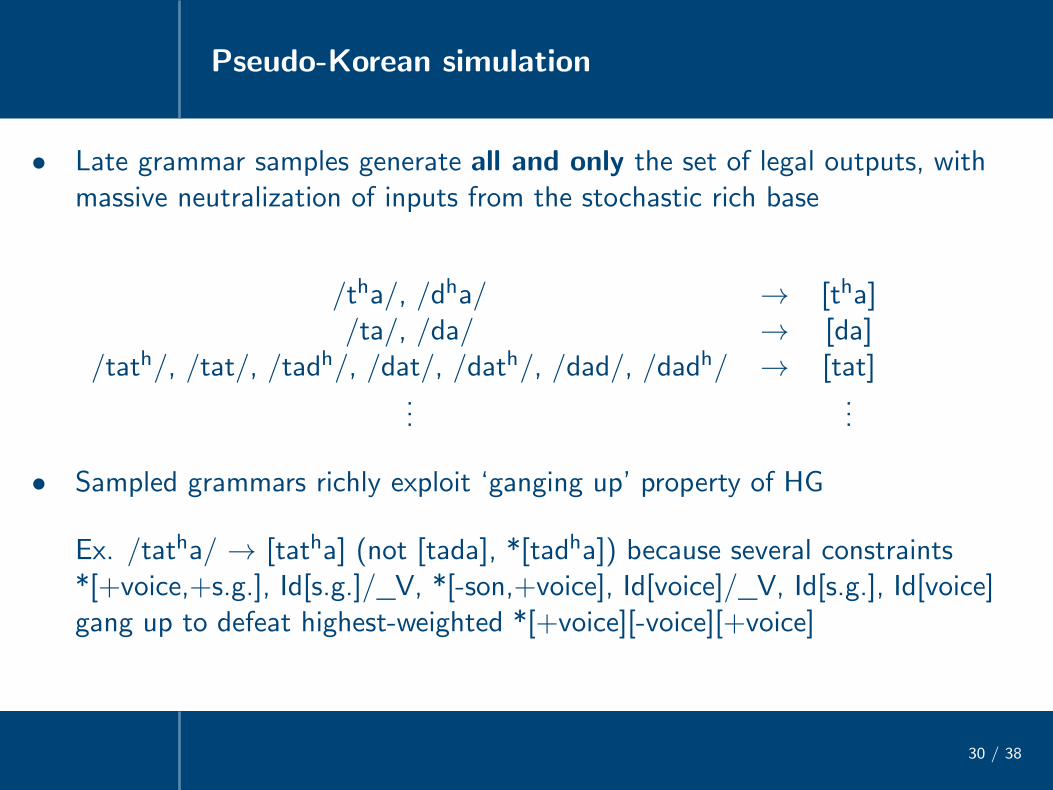
• Late grammar samples generate all and only the set of legal outputs, withmassive neutralization of inputs from the stochastic rich base
/tha/, /dha/ → [tha]/ta/, /da/ → [da]
/tath/, /tat/, /tadh/, /dat/, /dath/, /dad/, /dadh/ → [tat]...
...
• Sampled grammars richly exploit ‘ganging up’ property of HG
Ex. /tatha/ → [tatha] (not [tada], *[tadha]) because several constraints*[+voice,+s.g.], Id[s.g.]/ V, *[-son,+voice], Id[voice]/ V, Id[s.g.], Id[voice]gang up to defeat highest-weighted *[+voice][-voice][+voice]

AZBA simulation
31 / 38
AZBA language type (Prince & Tesar 2004, Hayes 2004)
• Laryngeal phonotactics of stops and fricatives
- Contrast between voiced and voiceless stops word-initial and word-finally[pa, ba, ap, ab]
- No contrast between voiced and voiceless fricatives[sa], [as] (*[za], *[az])
- Voiced fricatives occur allophonically under regressive voicing assimilation;voicing contrast in stops is neutralized under the same conditions[aspa], [azba], [apsa] (*[azpa], *[asba], *[absa], *[abza])
• ConstraintsM: AgreeVoice, NoVcdStop, NoVcdFricF: IdentVoiceStop, IdentVoiceStop/Onset
IdentVoiceFric, IdentVoiceFric/Onset

AZBA simulation
31 / 38
Weight samples (normalized to sum to unity)
0 100 200 300 400 500 600
0.05
0.10
0.15
0.20
0.25
0.30
sampling iteration (x10)
norm
aliz
ed c
onst
rain
t wei
ght
AgreeVoice
No(b)
No(z)
IdVoiceStop
IdVoiceStop/Ons
IdVoiceFricIdVoiceFric/Ons
AZBA simulation
31 / 38
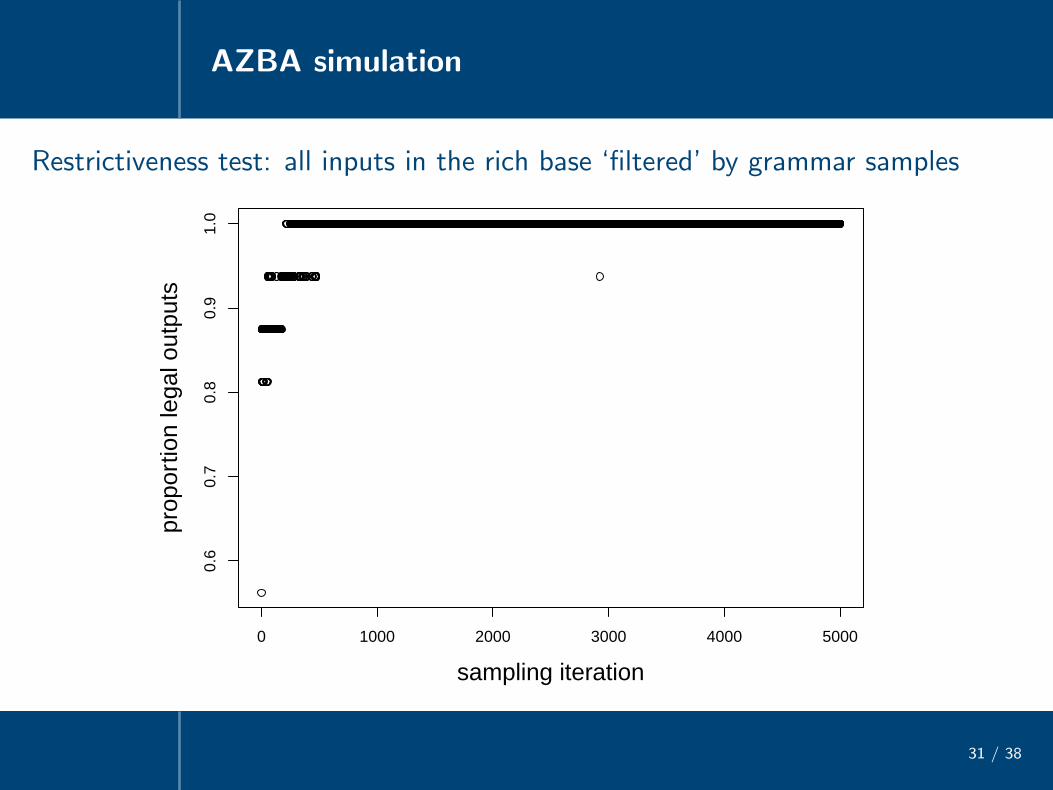
Restrictiveness test: all inputs in the rich base ‘filtered’ by grammar samples
0 1000 2000 3000 4000 5000
0.6
0.7
0.8
0.9
1.0
sampling iteration
prop
ortio
n le
gal o
utpu
ts
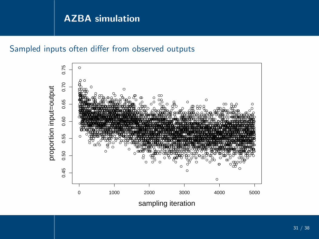
AZBA simulation
31 / 38
Sampled inputs often differ from observed outputs
0 1000 2000 3000 4000 5000
0.45
0.50
0.55
0.60
0.65
0.70
0.75
sampling iteration
prop
ortio
n in
put=
outp
ut

PAKA simulation
32 / 38
PAKA language type (Prince & Tesar 2004, Hayes 2004, Tessier 2007)
• Only initial-syllable vowels can be stressed (but not all are, perhaps because‘stress’ is actually pitch accent)
• Only stressed vowels contrast for length
[paka], [pa:ka], [paka] (*[paka], *[paka:], *[pa:ka], etc.)
• ConstraintsM: InitialStress, NoLongF: IdentStress, IdentLong, IdentLong/Stressed, IdentLong/Initial

PAKA simulation
32 / 38
Weight samples (normalized to sum to unity)
0 100 200 300 400 500 600
0.05
0.10
0.15
0.20
0.25
0.30
sampling iteration (x10)
norm
aliz
ed c
onst
rain
t wei
ght
InitialStress
NoLong
IdentStress
IdentLong
IdentLong/Stress
IdentLong/Initial
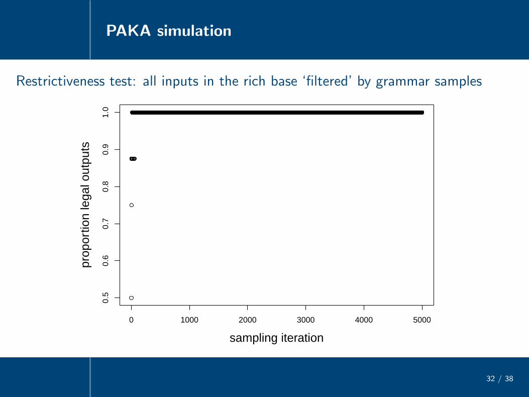
PAKA simulation
32 / 38
Restrictiveness test: all inputs in the rich base ‘filtered’ by grammar samples
0 1000 2000 3000 4000 5000
0.5
0.6
0.7
0.8
0.9
1.0
sampling iteration
prop
ortio
n le
gal o
utpu
ts
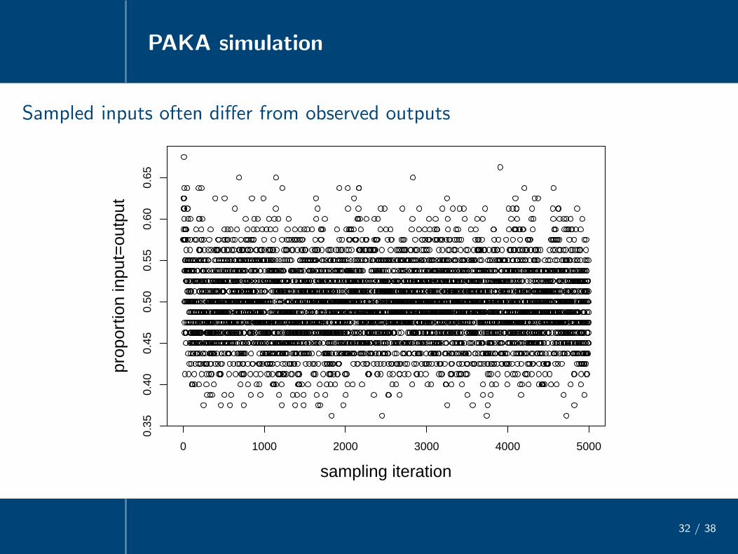
PAKA simulation
32 / 38
Sampled inputs often differ from observed outputs
0 1000 2000 3000 4000 5000
0.35
0.40
0.45
0.50
0.55
0.60
0.65
sampling iteration
prop
ortio
n in
put=
outp
ut
Restrictive grammars from an uninformative prior
33 / 38
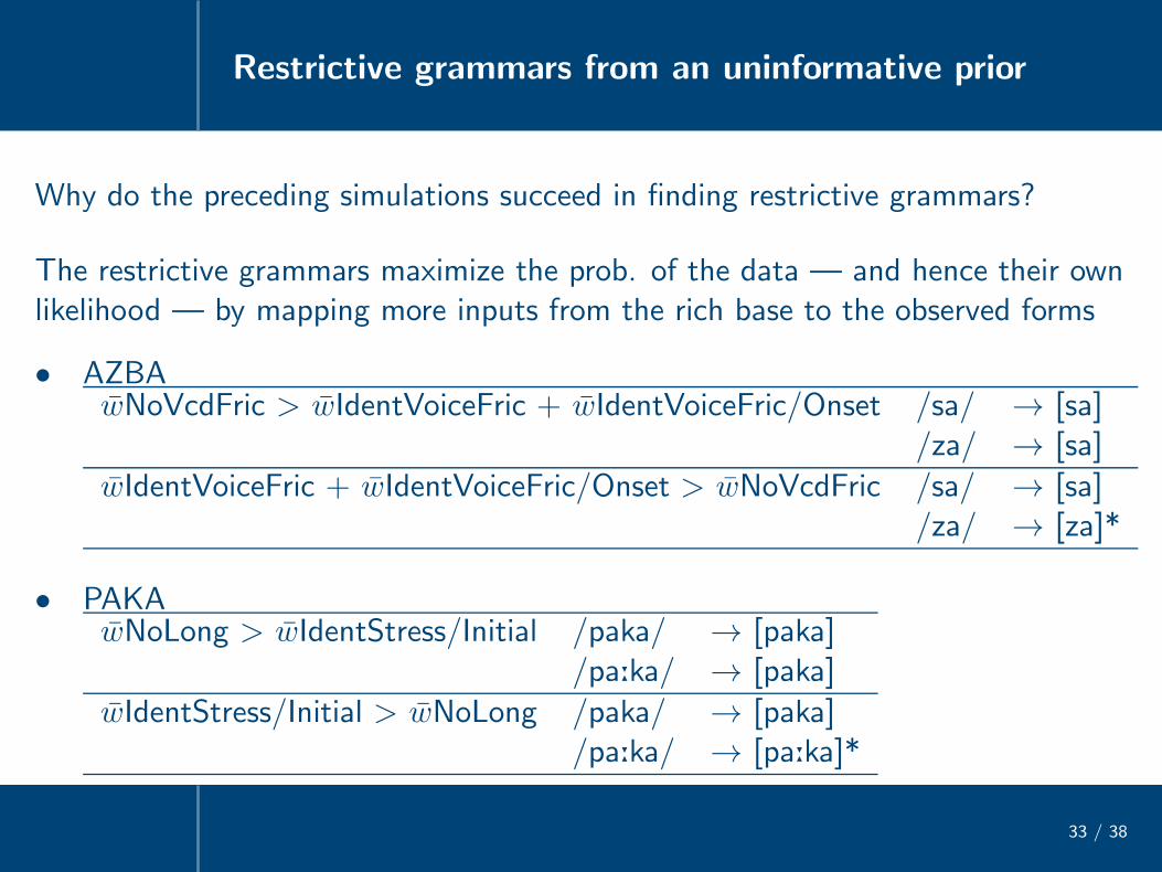
Why do the preceding simulations succeed in finding restrictive grammars?
The restrictive grammars maximize the prob. of the data — and hence their ownlikelihood — by mapping more inputs from the rich base to the observed forms
• AZBAwNoVcdFric > wIdentVoiceFric + wIdentVoiceFric/Onset /sa/ → [sa]
/za/ → [sa]
wIdentVoiceFric + wIdentVoiceFric/Onset > wNoVcdFric /sa/ → [sa]/za/ → [za]*
• PAKAwNoLong > wIdentStress/Initial /paka/ → [paka]
/pa:ka/ → [paka]
wIdentStress/Initial > wNoLong /paka/ → [paka]/pa:ka/ → [pa:ka]*

Restrictive grammars from an uninformative prior
33 / 38
The posterior distribution over grammars is the joint distribution marginalizedover all possible weight samples and inputs:
p(w|y) ∝
∫
W
∑
x
α(w,W,x,y)
where
α(w,W,x,y) = p(y|W,X) × p(W|w)
which can be thought of as a positive, fractional ‘point’ that grammar w receivesif the inputs in x are mapped to the observed outputs by the weights W
Grammars with larger point totals by def. have higher posterior probability

Restrictive grammars from an uninformative prior
33 / 38
Posterior/restrictiveness connectionMore restrictive grammars have higher posterior probability because they receivelarger probability contributions from more combinations of weights and inputs(similar ideas suggested by Paul Smolensky, p.c., pursued in Riggle 2006, Jarosz 2006, 2007)
• Only possible if Input assumption is relaxed
• If correct, renders Low IO-Faithfulness assumption and associatedlearning-specific mechanisms unnecessary
(see example on next slide)
Restrictive grammars from an uninformative prior
33 / 38
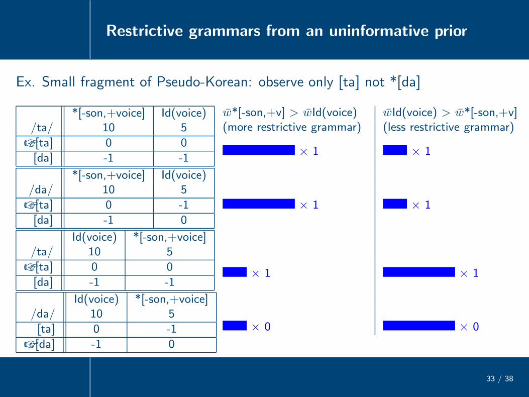
Ex. Small fragment of Pseudo-Korean: observe only [ta] not *[da]
*[-son,+voice] Id(voice)/ta/ 10 5
☞ [ta] 0 0
[da] -1 -1
*[-son,+voice] Id(voice)/da/ 10 5
☞ [ta] 0 -1
[da] -1 0
Id(voice) *[-son,+voice]/ta/ 10 5
☞ [ta] 0 0
[da] -1 -1
Id(voice) *[-son,+voice]/da/ 10 5
[ta] 0 -1
☞ [da] -1 0
w*[-son,+v] > wId(voice) wId(voice) > w*[-son,+v](more restrictive grammar) (less restrictive grammar)
× 1 × 1
× 1 × 1
× 1 × 1
× 0 × 0

Restrictive grammars from an uninformative prior
33 / 38
Summary: two-part strategy for guaranteeing grammatical restrictiveness in earlyphonological learning
• Learning objective: sample from the posterior distribution over grammars
- Gibbs sampler guaranteed to do this given sufficient time
- Quite possibly other sampling methods would be even more efficient
• Posterior/restrictiveness connection
- Prove that grammars with higher posterior probability are more restrictive
- Trivial given the uninformative prior if more restrictive ⇔ higher likelihood(see Jarosz 2006, 2007 for relevant discussion and proof of a simple case)
Extensions
34 / 38
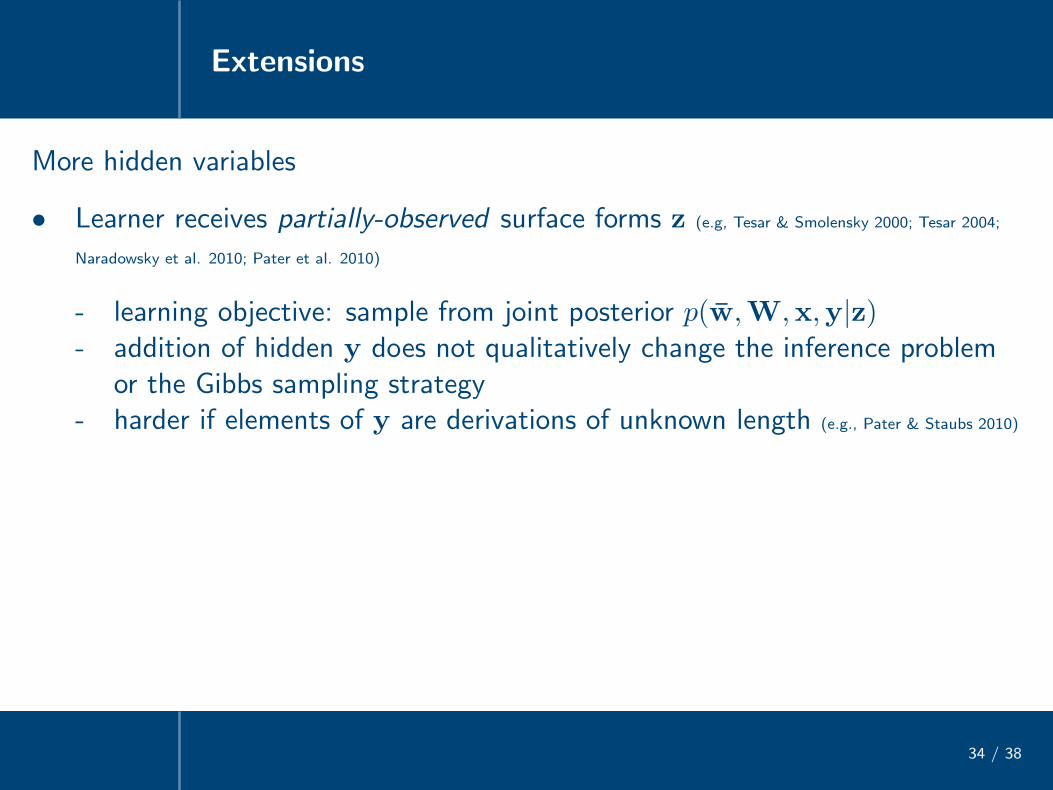
More hidden variables
• Learner receives partially-observed surface forms z (e.g, Tesar & Smolensky 2000; Tesar 2004;
Naradowsky et al. 2010; Pater et al. 2010)
- learning objective: sample from joint posterior p(w,W,x,y|z)- addition of hidden y does not qualitatively change the inference problem
or the Gibbs sampling strategy- harder if elements of y are derivations of unknown length (e.g., Pater & Staubs 2010)
Extensions
34 / 38
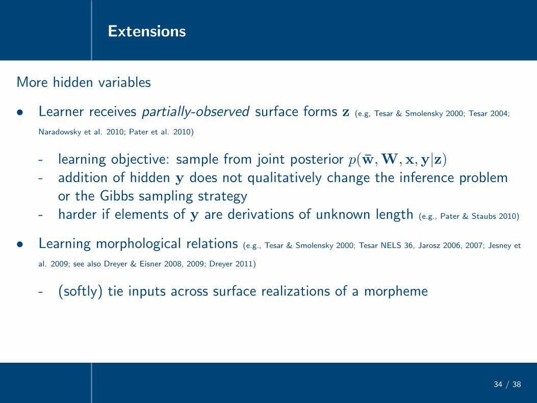
More hidden variables
• Learner receives partially-observed surface forms z (e.g, Tesar & Smolensky 2000; Tesar 2004;
Naradowsky et al. 2010; Pater et al. 2010)
- learning objective: sample from joint posterior p(w,W,x,y|z)- addition of hidden y does not qualitatively change the inference problem
or the Gibbs sampling strategy- harder if elements of y are derivations of unknown length (e.g., Pater & Staubs 2010)
• Learning morphological relations (e.g., Tesar & Smolensky 2000; Tesar NELS 36, Jarosz 2006, 2007; Jesney et
al. 2009; see also Dreyer & Eisner 2008, 2009; Dreyer 2011)
- (softly) tie inputs across surface realizations of a morpheme
Extensions
34 / 38
More hidden variables
• Learner receives partially-observed surface forms z (e.g, Tesar & Smolensky 2000; Tesar 2004;
Naradowsky et al. 2010; Pater et al. 2010)
- learning objective: sample from joint posterior p(w,W,x,y|z)- addition of hidden y does not qualitatively change the inference problem
or the Gibbs sampling strategy- harder if elements of y are derivations of unknown length (e.g., Pater & Staubs 2010)
• Learning morphological relations (e.g., Tesar & Smolensky 2000; Tesar NELS 36, Jarosz 2006, 2007; Jesney et
al. 2009; see also Dreyer & Eisner 2008, 2009; Dreyer 2011)
- (softly) tie inputs across surface realizations of a morpheme
• Learning constraints (e.g., Pater & Staubs 2010; Hayes & Wilson 2008; Pater, to appear)
- learning objective: sample from joint posterior p(Con, w,W,x, |z) ?!
Extensions
35 / 38
Different constraint-based formalisms
• Noisy OT
- learning objective and inference strategy remain largely the same- feasibility depends on parameterization of ranking probabilities
(e.g., Boersma 1997, Boersma & Hayes 2001 vs. Jarosz 2006, 2007)
• Conditional maximum entropy
- easier inference problem: no need for weight samples W, becausegrammars are inherently stochastic
In the near future: comparison of multiple constraint-based grammaticalframeworks on learning-theoretic grounds (see already Jesney 2009)
Extensions
36 / 38
Later stages of phonological acquisition
• Many proposals assume (at least partly) distinct grammars for perception andproduction (e.g., Smith 1973; Demuth 1995, 1996; Pater & Paradis 1996; Boersma 1998; Pater 2004; Hayes 2004; Jarosz
2006, 2007; cf. Smolensky 1996)
- broadly supported by neurophysiological and neuropsychological evidencefor distinct input and output lexicons and processing in adults(e.g., Hickok 2000, Poeppel & Hickok 2004, 2007; Guenther 1995; Guenther et al. 1998, 2006; Shallice 2000)
- production grammar maps adult-like surface representation to child form(e.g., Smith 1973; Demuth 1995; Gnanadesikan 1995; Pater & Paradis 1996; Levelt and Van de Vijver 1998; Hayes 2004)
• Tentative proposal: train initial production grammar from perceptiongrammar by mapping all adult surface forms to silence (null output)
p(wprod) ∝ sim(wprod, wperc)× δ(null outputs|wprod)
Summary
37 / 38
• Bayesian inference of (sampling from) the posterior distribution on noisyHarmonic Grammars can be achieved with modern MCMC techniques
• More restrictive grammars in test cases have higher posterior probability,despite the unbiased prior, because they receive support from morecombinations of the hidden variables (= weight samples, inputs)
- supported by replicable simulations- difficulty of general proof hinges on def. of ‘restrictive’
• Pursuing simplification in learning theory
- avoid learning-specific assumptions- embrace learner’s ignorance of hidden variables- pursue consequences of inference with an unbiased prior
Thank you!
38 / 38