COHERENT FIBER OPTIC TEMPERATURE SENSOR · TELECOMMUNICATION ENGINEERING ... Fig. 4.2.2.3.5...
77
COHERENT FIBER OPTIC TEMPERATURE SENSOR A Thesis Report Submitted to The Department di Elettronica, Informazione e Bioingegneria POLITECNICO DI MILANO, MILANO, ITALY In partial fulfilment for the award of degree of MASTER OF SCIENCE IN TELECOMMUNICATION ENGINEERING Supervisor: Prof. Mario Martinelli Co-Supervisor: Dott. Ing. Maddalena Ferrario Submitted By: Amitesh Singh 10449979 Department di Elettronica, Informazione e Bioingegneria Politecnico di Milano, P.zza L. da Vinci, 32, 20133 Milano, Italy DECEMBER 2015
Transcript of COHERENT FIBER OPTIC TEMPERATURE SENSOR · TELECOMMUNICATION ENGINEERING ... Fig. 4.2.2.3.5...

COHERENT FIBER OPTIC TEMPERATURE SENSOR
A
Thesis Report
Submitted to
The Department di Elettronica, Informazione e Bioingegneria
POLITECNICO DI MILANO, MILANO, ITALY
In partial fulfilment for the award of degree of
MASTER OF SCIENCE
IN
TELECOMMUNICATION ENGINEERING
Supervisor:
Prof. Mario Martinelli
Co-Supervisor:
Dott. Ing. Maddalena Ferrario
Submitted By:
Amitesh Singh 10449979
Department di Elettronica, Informazione e Bioingegneria Politecnico di Milano, P.zza L. da Vinci, 32, 20133 Milano, Italy
DECEMBER 2015
[i]
POLITECNICO DI MILANO
P.zza L. da Vinci, 32, 20133 Milano, Italy
Phone: 800.02.2399 Fax: +39.02.2399.2206
Website: www.polimi.it
CERTIFICATE
This is to certify that “Amitesh Singh 814999 (10449979)” students of
Telecommunication Engineering from “POLITECNICO DI MILANO, ITALY” has
done their Thesis at “Politecnico di Milano, Milano, ITALY” in the partial fulfilment
for the award of degree of “Master of Science” under the guidance of “Prof. Mario
Martinelli” and “Dott. Ing. Maddalena Ferrario”
The project work entitled as “COHERENT FIBER OPTIC TEMPERATURE
SENSOR” embodies the original work done for Thesis. This work has not been
submitted partially or wholly to any other university or institute for the award of this or
any other degree.
Prof. Maurizio Magarini
The Department di Elettronica, Informazione
e Bioingegneria.
Dott. Ing. Maddalena
Ferrario
[ii]
ACKNOWLEDGEMENT
I would like to thank all those who gave us the possibility to complete this Thesis. I want
to thank the Department di Elettronica, Informazione e Bioingegneria of
“POLITECNICO DI MILANO” for giving us such a golden opportunity to commence
this Thesis in first instance. I express our deepest gratitude to “Prof. Mario Martinelli”
who encouraged me to go ahead with Thesis. It is a matter of pride and privilege for us to
complete our dissertation under his close supervision. Whatever is said in the praise of
Prof. Mario Martinelli is not enough, his soul touching humility, his straight forward
attitude, his methodological approach, his eagerness to share his wisdom, his aim for
perfection and his never ending encouragement and patience are but a few of his noble
qualities. It is certainly good karma to have Dott. Ing. Maddalena Ferrario for
supervising our work as his advice, his words of wisdom and valuable guidance have
allowed the completion of our work without any hassle.
We are also very grateful to Ing. Marco Mattarei, for the facilities and cooperation; he
provided me guidance in the completion of Thesis work. I also express our deepest gratitude
to “Ing. Marco Mattarei”. Our special appreciation goes to teachers, who has inspired and
guided us during seven months in this institution by their brilliant and expert teaching. We
gratefully acknowledge the help and cooperation extended by the library staff of the faculty
as well as university. Our heart gratitude goes to our parents and all friends for their
invaluable inspiration extended in the pursuit of this work.
………………………
Amitesh Singh
[iii]
DECLARATION BY SCHOLAR
I hereby declare that the work reported in my M.Sc. thesis entitled as “Coherent Fiber
Optic Temperature Sensor,” submitted at Department Di Elettronica, Informazione e
Bioingegneria, Politecnico di Milano, is an authentic record of our research work
carried out under the supervision of Prof. Mario Martinelli and Dott. Ing. Maddalena
Ferrario. I have not submitted this work elsewhere for any other degree.
……………………………..
Amitesh Singh
(814999)

[iv]
List of Abbreviations
S. No. Abbreviation Description
1. FBG Fiber-Bragg-Grating
2. FRM Faraday Rotation Mirrors
3. DFB Distributed Feedback Laser
4. VCSEL Vertical-Cavity Surface-Emitting Laser
5. EMI Electromagnetic Interference
6. WDM Wavelength-Division Multiplexing
7. GMM Giant Magnetostrictive Materials
8. FRIS Free Running Interferometric Sensor
9. FM Frequency modulation
10. RTM Real-Time Measurements
11. HT High Temperature
12. EFPI Extrinsic Fabry-Pérot interferometric
13. DFPI Diaphragm-based Fabry-Perot Interferometric
14. FOS Fiber Optic Sensor
15. LB Large Bandwidth
16. HS High Sensitivity
17. CPS Conventional Pressure Sensors
18. HF High Frequency
19. HR High Reliability
20. IS Intrinsic Sensors
21. ES Extrinsic Sensors
22. TD Time delay
23. OTD Optical Time-Domain
24. OFD Optical Frequency Domain
25. LFG Long-period Fiber Grating
26. MRI Magnetic Resonance Imaging
27. DTS Distributed Temperature Sensing
28. RTD Resistance Temperature Detectors
29. II Extrinsic Interferences
30. EI Intrinsic Interferences
[v]
31. FODS Fiber Optic Displacement Sensor
32. POF Plastic Optical Fiber
33. SMF Single-Mode Fiber
34. MMF Multi-Mode Fiber
35. BFL Brillouin Fiber Laser
36. OTDR Optical Time Domain Reflectometry
37. OFDR Optical Frequency Domain Reflectometry
38. FFT Fast Fourier Transform
39. WSR Wavelength-Specific Reflector
40. AFC Anti-Reflective Coating
41. PMT Photomultiplier Tubes
42. IFS Interferometric Fiber Sensor
43. PMFS Phase-Modulated Fiber Sensor
44. FOIS Fiber Optic Interferometric Sensors
45. RI Refractive Index
46. OWN Optical Wave Number
47. OPD Optical Phase Delay
48. SA Sensing arm
49. RA Reference arm
50. DC Direct Coupling
51. IDC Indirect Coupling
52. QPS Quadratic-Phase Signal
53. TDF Time-Domain Function
54. FDF Frequency-Domain Function
55. LD Laser Diode
56. LED Light-Emitting Diode
57. FOC Fiber Optic Communications
58. ILD Injection Laser Diode
59. DBR Distributed Bragg Reflector
60. DQE Differential Quantum Efficiency
61. HRM High Reflectivity Mirrors
62. EEL Edge-Emitting Lasers
63. VCSOA Vertical-Cavity Semiconductor Optical Amplifiers

[vi]
64. TDL Tunable Diode Laser
65. SMSR Side Mode Suppression Ratio
66. NPB Narrow Pass Band
67. LED Light-Emitting Device
68. TEC Thermoelectric Cooler
69. RTO Real Time Oscilloscope
70. FOCT Fiber Optic Coherent Technology
71. QP Quadrature Point
72. FRM Faraday Rotation Mirrors
73. OSW Optical Source Wavelength
74. LT Local Temperature

[vii]
List of Symbols
S. No Symbols Description
1 λB Bragg wavelength
2 ne Effective refractive index of the grating in the
fiber is core
3 Λ Grating period
4 ∆λ Bandwidth
5 ᵟn0 Variation in the refractive index
6 Lg Grating length
7 PB(λB) Peak reflection
8 N Number of periodic variations
9 PB(λ) Reflected power
10 Φ Optical phase delay
11 n Refractive index of the fiber core
12 k Optical wave number
13 L Physical length of the fiber
14 Pd Photodiode
15 c Velocity of light
16 n∆L Optical path difference
17 ξ Strain optic correction factor
18 μ Poisson’s ratio, and
19 pij Elements of the strain optic tensor
20 𝑓(𝑡) Instantaneous frequency
21 𝑘 Rate of frequency increase or chirp rate
22 Φ ′(t) Angular frequency

[viii]
List of Figure
S. No. Figure no. Caption of the Figure Page
No.
1. Fig. 1.1.1 2x2 Coupler Schematic 3
2. Fig. 1.1.2 3x3 Optical Fiber Coupler 4
3. Fig. 2.2 Over-view of DFB 12
4. Fig. 2.3.1 FBG Overview 14
5. Fig. 2.3.2 FBG Core Refractive Index 14
6. Fig. 2.3.3 FBG Spectral Response 15
7. Fig. 2.4 FPI Fringes 16
8. Fig. 2.4.2 Single Fiber Intensity Sensor 18
9. Fig. 2.4.2.2.1 DIS 19
10. Fig. 2.4.2.2.2 Elastooptic Modulation 20
11. Fig. 2.4.3 Overview of Interferometric 21
12. Fig. 3.1.1 Interference block diagram 23
13. Fig. 3.1.2 Block Diagram for Interferometry 24
14. Fig. 3.1.3 3x3 Fiber Coupler 25
15. Fig. 3.2 Output Response for Interferometry. 28
16. Fig. 4.2.2.2.1 DFB Active Region 38
17. Fig. 4.2.2.2.2 DFB Region 40
18. Fig. 4.2.2.2.3 DFB Response 40
19. Fig. 4.2.2.3.1 14-Pin Butterfly Mount 42
20. Fig. 4.2.2.3.2 Tocan Laser 42
21. Fig. 4.2.2.3.3 To-can pin alignment 43
22. Fig. 4.2.2.3.4 Description of package 43
23. Fig. 4.2.2.3.5 Structural blue print of fiber 44
24. Fig. 5.1.1.1 Simulation for fringes with fiber length 45
25. Fig. 5.1.1.2 Simulation for fringes depends on wavelength 45
26. Fig. 5.1.1.3 Simulation for temperature depend fringes 46
27. Fig. 5.1.1.4 Simulation for different temperature & fringes vary 46
28. Fig. 5.1.2.1 Chirp setup 47
30. Fig. 5.1.2.2 Setup configuration 47
[ix]
31. Fig. 5.1.3 Vcsel result 48
32. Fig. 5.1.4.1 DFB result 49
33. Fig. 5.1.4.2 Tocan result 50
34. Fig. 5.1.4.3 Simulation result for DFB & To-can 50
35. Fig. 5.2.1.1 Coupler setup 51
36. Fig 5.2.1.2 Setup for 3x3 coupler 52
37. Fig 5.2.1.3 Fiber dip in water with heating 52
38. Fig. 5.2.2.1 Different temperature 53
39. Fig.5.2.2.2 Mean & Std with different temperature 54
40. Fig. 5.2.2.3 Simulation for 20 – 75o 55

ABSTRACT
In many industrial application fields (oil & gas and high voltage transformers…) the
use of conventional electrical temperature sensors (e.g. thermocouples) is forbidden
because of harsh environmental conditions or risk of explosions due to sparks. In
these fields fiber optic sensor represent a valid alternative as they can withstand
severe conditions (high temperature, pressure) and offer a complete electromagnetic
immunity.
Already available commercial fiber optic temperature sensors are mainly of two types:
distributed sensors, that is, they can provide the entire profile of temperature along the
entire fiber length (even km) with high spatial resolution (Raman, Brillouin sensor).
And local sensors is that, in this case the fiber is used only to transport the optical light
but the actual sensor is a material with peculiar thermal properties (fluorescence,
absorption) which is place on top of the fiber end face.
These commercial systems are still expensive monitoring solutions and their cost can
only be sustained mainly by industries such those of the Oil & Gas and High-Voltage
Transformers.
On the other hand, the Manufacturing Industry (packaging, mechanical, automotive…)
is now realizing the importance of implementing predictive maintenance strategies to
prevent the occurrence of failure and downtimes in the manufacturing process. The
implementation of an effective predictive maintenance requires the installation of
monitoring system comprising a plurality of conventional sensors (even temperature
sensors) which can provide manifold real-time information on the machine condition.
The manufacturing industry is however struggling with the still high costs and
complexity of installation of these monitoring solutions based on conventional
electrical sensors.
In this frame fiber optic sensors can bring a real innovation, due to their minimal
invasiveness, electromagnetic immunity and capability to sense manifold
environmental parameter with the same transducer, that is, the optical fiber. As
mentioned above commercially available fiber optic sensors are however too
expensive.
In the present work, we have decided to re-consider a coherent approach, that is,
interferometric, to fiber optic sensors, to achieve a cost-effective solution that can be
proposed also to the Manufacturing Industry.
Interferometric technique were already proposed more than 40 years ago, offering
very high sensitivity and accuracy, but their actual in-field applicability has been limited
by technological issues related to the stabilization of the interferometric working point
and polarization fading.

In the present work to overcome, the above-mentioned issues a completely passive
phase diversity receiver combined with Faraday rotation mirrors, respectively for
quadrature point and polarization stabilization, have been exploited to develop a low-
cost interferometric fiber optic sensor capable to reliably detect temperature variations
in an industrial environment.
The present work are divided as follows: in the first chapter, a brief review of the fiber
optic sensor peculiar properties is given while in the second chapter a more detailed
description is provided related to fiber optic temperature sensors. In the third chapter
a theoretical description of the coherent approach to fiber optic sensing is given. In
particular, in order to convert temperature measurement which is a quasi-static
parameter, in a dynamic measurement, which guarantees a better accuracy, coherent
detection is associated with a wavelength modulation, that is, a chirp of the optical
laser source. In chapter four different typology of laser source with different chirp
characteristics are taken into account and compared to evaluate the optical source
that allows better performance in terms of sensitivity and accuracy in coherent
detection. Finally, in chapter five, the coherent fiber optic temperature sensor
experimental setup is described and preliminary results are provided.

ABSTRACT
In molti settori industriali diversi campi di applicazione (oil & gas e trasformatori di alta
tensione…) l'uso di tradizionali elettriche dei sensori di temperatura (ad esempio
termocoppie) è vietato a causa delle severe condizioni ambientali o il rischio di
esplosioni dovute a scintille. In questi campi sensore a fibra ottica rappresentano una
valida alternativa in quanto possono resistere a condizioni difficili (ad alta temperatura,
pressione) e offrono una completa immunità elettromagnetica.
Già disponibile in commercio sensori di temperatura in fibra ottica sono principalmente
di due tipi: sensori distribuiti, che essi possono fornire tutto il profilo di temperatura
lungo tutta la lunghezza della fibra (anche km) con elevata risoluzione spaziale
(Raman, Brillouin sensore). E sensori locali è che in questo caso la fibra viene
utilizzato solo per il trasporto della luce ottica ma il sensore effettivo è un materiale
con una peculiare proprietà termiche (fluorescenza, assorbimento) che è posto sulla
cima di la faccia finale della fibra.
Questi sistemi commerciali sono ancora costose soluzioni per il monitoraggio e il loro
costo può essere sostenuta solo principalmente dalle industrie quali quelli dell'Oil &
Gas e trasformatori di alta tensione.
D'altro canto, l'industria manifatturiera (imballaggio, meccanica, automotive…) è ora a
rendersi conto dell importanza di attuare la manutenzione predittiva delle strategie per
prevenire il verificarsi del guasto e tempi morti nel processo di fabbricazione. La
realizzazione di un efficace manutenzione predittiva richiede l'installazione del sistema
di monitoraggio comprendente una pluralità di sensori convenzionali (anche sensori
di temperatura) che può fornire il collettore informazioni in tempo reale sulle condizioni
della macchina. L'industria manifatturiera è tuttavia lottando con gli ancora elevati costi
e complessità di installazione di queste soluzioni per il monitoraggio basato su
convenzionali sensori elettrici.
In questa cornice i sensori a fibra ottica può portare una vera innovazione, a causa
della loro invasività minima, immunità elettromagnetica e capacità di collettore di
rilevamento del parametro ambientale con lo stesso trasduttore, cioè la fibra ottica.
Come accennato in precedenza disponibili in commercio sensori a fibra ottica sono
però troppo costoso.
Nel presente lavoro abbiamo deciso di ri-considera un approccio coerente, che
è, interferometrico per sensori a fibre ottiche, per ottenere una soluzione conveniente
che può essere proposto anche per il settore manifatturiero.
Tecnica interferometrica sono stati già proposti più di quarant anni fa, offrendo molto
alta sensibilità e precisione, ma la loro effettiva nel campo di applicabilità è stata

limitata da problemi tecnologici legati alla stabilizzazione del interferometrica del punto
di lavoro e polarizzazione fading.
Nel presente lavoro di superare il sopra menzionato questioni completamente una
fase passiva di ricevitore in diversità combinata con la rotazione di Faraday specchi,
rispettivamente per punto in quadratura e la stabilizzazione di polarizzazione, sono
stati sfruttati per sviluppare un basso costo interferometriche di sensore a fibra ottica
in grado di rilevare in maniera affidabile le variazioni di temperatura in un ambiente
industriale.
Il presente lavoro sono suddivisi come segue: nel primo capitolo un breve riepilogo
del sensore a fibra ottica peculiari proprietà è dato mentre nel secondo capitolo una
descrizione più dettagliata è fornite relative ai sensori di temperatura in fibra ottica.
Nel terzo capitolo una descrizione teorica di un approccio coerente di rilevamento a
fibre ottiche è dato. In particolare, al fine di convertire la misura di temperatura che è
quasi un parametro statico in una misura dinamica, che garantisce una migliore
precisione, rilevamento coerente è associato ad una lunghezza d'onda di
modulazione, che è, un chirp dell'ottica laser sorgente. Nel capitolo 4 la diversa
tipologia di sorgente laser con diverse caratteristiche di pigolio sono presi in
considerazione e rispetto per valutare la sorgente ottica che consente di ottenere
prestazioni migliori in termini di sensibilità e precisione nel rilevamento
coerente. Infine nel capitolo cinque, la coerente in fibra ottica del sensore di
temperatura setup sperimentale è descritto e i risultati preliminari sono previsti.

CONTENTS
Certificate ………………………………………………………………………………….……...i
Acknowledgement ……………………………………………………………………………….ii
Declaration by Scholars ………………………………………………………………………..iii
List of Abbreviations ………………………………………………………………………...iv-vi
List of Symbols ………………………………………………………………………………….vii
List of Figures ………………………………………………………………………………..viii-ix
Abstract (English and Italian)………….…………………………………………………..x-xiii
1. INTRODUCTION AND MOTIVATION 1-7
1.1. Introduction 2-5
1.2. Motivation 6-7
2. FIBER OPTIC TEMPERATURE SENSOR 8-21
2.1. Fiber optic temperature sensors 8-11
2.1.1. Intrinsic Sensors 8-9
2.1.2. Extrinsic Sensors 9-11
2.2. Distributed Temperature Sensor 11-13
2.3. Fiber Bragg Grating 13-15
2.4. Local Temperature Sensors 15-21
2.4.1. Fabry–Pérot interferometer 15-16
2.4.2. Intensity sensors 16-20

2.4.3. Interferometric sensors 20-21
3. COHERENT TEMPERATURE FIBER OPTIC SENSOR 22-28
3.1. Theory of optical interferometry 22-25
3.2. Optical phase dependence on temperature 25-28
4. CHIRP MODULATION 29-44
4.1. Laser Chirp Modulation 29-31
4.1.1. Linear Chirp 29-30
4.1.2. Exponential Chirp 30-31
4.2. Laser Diodes 31-44
4.2.1. Operation 31-32
4.2.2. Different type of laser diodes 32-44
4.2.2.1. VCSEL 33-36
4.2.2.1.1. Structure 33-35
4.2.2.1.2. Characteristics 35-36
4.2.2.2. Distributed Feedback Laser 36-41
4.2.2.3. Laser Diode Packaging 42-44
5. SIMULATIONS AND EXPERIMENTAL RESULTS 45-57
5.1 Chirp impact on phase fringes measurement 45-50
5.1.1. Phase-Chirp Simulation 45-46
5.1.2. Chirp Measurement Setup 47-48
5.1.3. VCSEL Laser chirp 48-49
5.1.4. DFB\To-can Laser chirp 49-50
5.2. Coherent fiber optic temperature sensor 51-55

5.2.1. Experimental setup with 3x3 coupler 51-52
5.2.2. Temperature experimental characterisations 53-55
6. CONCLUSIONS 56-57
REFERENCES
CHAPTER 1 INTRODUCTION AND MOTIVATION
Department di Elettronica, Informazione e Bioingegneria Politecnico di Milano, P.zza L. da Vinci, 32, 20133 Milano, Italy
1
1.1 Introduction
In many fiber optic sensors, the fiber simply carries the light to the remote
optical sensor at the end of the fiber. The light is then somehow modified and returned,
typically through the same fiber, to the source module, where it is analyzed. This type
of sensor is usually referred to as an intensity-type fiber sensor, and as stated, the
fiber plays no role in the sensing mechanism. With these sensors, light typically has
to leave the optical fiber to interact with the optical sensor at the end of the fiber, in
many instances leading to substantial optical loss. There is, however, another class of
fiber sensor where the fiber plays a more intimate role with the sensing mechanism,
and the light is not required to exit the fiber at the sensor to interact with the field to be
detected. In this type of device, the optical phase of the light passing through the fiber
is modulated by the field to be detected. This phase modulation is then detected
interferometrically, by comparing the phase of the light in the signal fiber to that in a
reference fiber. This type of sensor has a number of attractive features. As the light
remains in the fiber, the device usually has a very low optical loss, and because the
device uses the interference of light, it is very sensitive. Through a number of
mechanisms, the optical phase of the light passing through a fiber may be made
sensitive to many parameters. It is also possible to multiplex this type of sensor very
efficiently. This type of sensor is referred to as a phase-modulated or interferometric
fiber sensor.
Fiber optic interferometric sensors, as well as having the advantages generally
attributed to fiber sensors, such as electrically passive (safety), lightweight, immunity
to electromagnetic interference (EMI), and multiplexing, have the additional
advantages of geometric versatility of the sensing element, wide dynamic range, and
extremely high sensitivity, It is worthwhile to describe in greater detail the form of some
of these advantages. For an acoustic sensor, where approximately 30m of fiber is
required for the acoustic element, the fiber could be wrapped so as to form a small
golf-ball-sized omnidirectional hydrophone, or the element could be configured as a
highly directional element of 30m length—or any size between these two extremes.
As will be shown, fiber interferometric sensors can detect strains up to 10-13 to 10-15;
this is the origin of their high sensitivity and wide dynamic range.
Consequently, there has been an intense research effort over the last 10 years to
develop sensors that capitalize on these advantages. However, it is some of these
“advantages” that have tended to slow the progress of this very promising technology.
For instance, the ability to make the fiber sensitive to many different parameters leads
to the problem of sensor selectivity. Acoustic sensors become accelerometers,
accelerometers become temperature sensors, and magnetometers become
CHAPTER 1 INTRODUCTION AND MOTIVATION
Department di Elettronica, Informazione e Bioingegneria Politecnico di Milano, P.zza L. da Vinci, 32, 20133 Milano, Italy
2
seismometers, which for high-performance, state-of-the-art sensors is undesirable.
Another major difficulty is that while the relationship between the optical phase shift
and the parameter to be detected is linear over many orders of magnitude, the output
of the interferometer, owing to the “raised-cosine fringes,” requires processing, which
can limit dynamic range, degrade performance, and elevate the noise floor of the
system.
The very high performance of the sensors also dictates stringent requirements on the
multiplexing of these sensors, so as to retain the system’s integrity with regard to
performance & the basic principle of operation of these sensors is described: two
beam interferometry. Two of the basic methods of interferometer demodulation are
described. First is the active homodyne approach, which although not applicable to
most real-world systems has had widespread use in the laboratory and may be
described as the “beginners’” demodulator. Incidentally, in the laboratory environment,
this approach has the lowest noise floor typically achievable with these sensors. Unlike
the active scheme, the second demodulation approach has no electrical components
in the interferometer and because of this and the fact that the approach does not form
a feedback loop to the interferometer, this is termed a passive approach. This and
other passive approaches have had widespread use outside the laboratory. Some of
the basic noise sources are also described here, including a brief discussion of
semiconductor diode laser noise properties, as this is one of the most commonly used
sources in fiber optic interferometric sensors. The problem of polarization fading is
then described, and various approaches to overcome this problem are discussed.
In Section 2.1, we describe various interferometer configurations: Mach–Zehnder,
Michelson, reflectometric, and Fabry–Perot. Also, a number of implementations, such
as gradiometers and push–pull designs, are discussed. Finally, some of the most
important applications of this technology are described. The most important group are
those involving ac measurements and include strain, acoustic, and acceleration.
Owing to thermally induced phase shifts in the interferometer, direct dc measurements
of parameters are difficult. Techniques that permit interferometers to measure dc
parameters are also described.
Fused fiber couplers are key devices in optical communications and optical fiber
sensor systems that either combine or split optical signals [1-5]. The continuous in-
line structure of these devices offers many attractive features, such as a low insertion
loss, low back reflection, good mechanical reliability, and no interface problems with
other fiber systems. A typical 2×2 fused fiber coupler is made by heating and pulling
two single mode fibers. The two separate fibers are fused into a combined and tapered
body. The fused fiber coupler can perform many important functions, including optical
power dividing, wavelength selective coupling and polarization splitting [6,7]. The
desired characteristics of the coupler can be controlled through proper control of the

CHAPTER 1 INTRODUCTION AND MOTIVATION
Department di Elettronica, Informazione e Bioingegneria Politecnico di Milano, P.zza L. da Vinci, 32, 20133 Milano, Italy
3
tapered length. The spectral selectivity is an important property to achieve high
sensitivity, high precision and high reliable sensing technology because the spectral
response is immune to any optical source instability or optical loss in the fiber [8]. This
study examined the feasibility of a 2×2 fused fiber coupler as a fiber optic sensor based
on its spectral transmission. The taped region was covered with a thermo-optic
external medium. The key hypothesis was that the transmission and coupling
characteristics of the coupler can interact with the external medium through
evanescent wave coupling. The environmental temperature affects the refractive index
of the external medium, which can cause a shift in spectral transmission. Theoretical
analysis predicted the device structural condition needed to achieve high sensitivity
and explained the behavior of the sensor device. The feasibility for practical
applications is also discussed.
Fig. 1.1.1 2x2 Coupler Schematic
Magnetic field sensors have been employed for a variety of applications, including
magnetic anomaly detection, magnetic compass, mineral prospecting, noncontact
switching, current measurement, and so on [1]. Fiber-optic sensors have been
implemented to detect magnetic fields by using Faraday effect [2,3], fiber Bragg
grating (FBG) [4], and Fabry–Perot interferometer [5]. Fiber optic sensors based on
phase-modulating interferometers possess a high sensitivity, and can be employed to
detect extremely weak time-varying magnetic perturbations [6]. Interferometric fiber-
optic magnetic field sensors have been successfully developed for past few decades
[6]. Although a high resolution has been obtained, most of these sensors are
investigated by using active phase technique, especially the phase tracking
demodulation [7–10]. The phase tracking demodulation introduces a feedback
electrical signal, in which the measuring range is very narrow. The phase generated
carrier (PGC) demodulation is an alternative method, which exhibits a good linearity
in a large dynamic range [11]. However, this method requires a carrier signal, and the

CHAPTER 1 INTRODUCTION AND MOTIVATION
Department di Elettronica, Informazione e Bioingegneria Politecnico di Milano, P.zza L. da Vinci, 32, 20133 Milano, Italy
4
carrier frequency determines the upper frequency limit of the measured magnetic field.
Fiber-optic magnetic field sensors based on magnetostrictive materials were first
proposed in 1980 [12]. The strain in magnetostrictive materials induced by external
magnetic field is transferred to the fiber, which results in the phase shift between the
beams in the interferometer. Metallic glasses have been used in magnetic field
sensors instead of bare nickel to obtain a higher sensitivity [8]. Other kinds of materials
are also implemented to detect magnetic field, such as ceramic materials [9],
amorphous ferromagnetic alloys [10], rare-earth giant magnetostrictive materials
(GMMs)[13], and so on. GMMs have attracted tremendous interests for a few years
because of their giant magneto strain in response to magnetic fields. Fortunately,
these unfavorable characteristics can be reduced by introducing a proper bias
magnetic field and a compressive prestress [14,15]. In this paper, an all-fiber magnetic
field sensor is proposed for detecting the weak alternating magnetic field. The sensor
is constructed in a fiber-optic Mach–Zehnder interferometer, and one arm of the
interferometer is wrapped on a magnetic transducer. A 3 × 3 coupler is used in the
interferometer to demodulate interferometric signals for recovering dynamic phase
shifts. Distinct from the active phase demodulation, this 3 × 3 coupler based
demodulation operates without any electrical signal. Besides, the 3 × 3 coupler based
passive demodulation is quite suitable for high frequency measurements.
Experimental results show that the sensor exhibits excellent linearity, good
reversibility, and high sensitivity.
Fig. 1.1.2 3x3 Optical Fiber Coupler
The use of a fiber-optic Mach-Zehnder interferometer to measure differences in
temperature or pressure between two single-mode fiber arms is described.
Temperature or pressure changes are observed as a motion of an optical interference
fringe pattern. Values are calculated for the pressure and temperature dependence of
the fringe motion. Pressure and temperature measurements are made with the
interferometer, and the experimental values for sensitivity.
CHAPTER 1 INTRODUCTION AND MOTIVATION
Department di Elettronica, Informazione e Bioingegneria Politecnico di Milano, P.zza L. da Vinci, 32, 20133 Milano, Italy
5
Today the fiber Bragg grating (FBG) is the component widely used for temperature
sensing. It takes advantage of the broad fiber communication band by using WDM
technology. However FBG sensing systems need very expensive wavelength
demodulation equipment and the cost of FBGs is still a little high. In this paper a simple
temperature sensor based on fiber coupler is demonstrated. A conventional bare fiber
coupler is packaged into a silica V groove, and its optical power splitting ratio is less
sensitive to the surrounding temperature [6]. To enhance the temperature sensitivity
of the fiber coupler, it was coated with organic–inorganic solgel film around the
coupling region. Because of the organic dopants among the network of silica material,
solgel film has a higher thermo-optical coefficient. As the ambient temperature varies,
the changed refractive index of the coating film of the coupler leads to variation of
coupling coefficient. Thus, temperature can be determined by monitoring the power
ratio of the coupler. Compared with FBGs [7], the fiber coupler has the advantages of
low cost, easy sensing signal processing, and good sensitivity after it is coated.
Couplers are much simpler, and their fabrication technology is more mature.
Describe two dynamic interferometric techniques based on the use of electrically
tunable lasers for measuring optical path length and path length changes. In one case
it has recently been shown1 that with the use of a rapidly tunable laser, dc drifts and
low frequency phase noise can be eliminated from an interferometer by an active
stabilization scheme. Several other authors [2-5] have proposed and demonstrated
other feedback schemes to obtain a similar effect. However, in some applications it
will not be feasible or even desirable to stabilize the interferometer. For example, if the
laser is to drive several independent interferometers, the stabilization scheme cannot
be used. In the first of the two schemes described in this paper we will show that using
a Free Running Interferometric Sensor (FRIS), which incorporates a rapidly tunable
laser, it is possible to extract information from the sensor independently of dc drifts
and low frequency phase noise. The FRIS system utilizes a passive interferometer,
which is desirable in remote sensing applications, and the system also allows for the
same laser source to drive several sensors simultaneously.
The second interferometric measurement scheme is a true FM technique, where the
information signal is carried in the frequency channel of the detected light signal; it is
suited for noncontact real-time measurements of refractive index or length of
transparent materials.
It is becoming widely recognized that various types of sensor can be advantageously
made by using optical fibers either as the medium for data transmission, or as the
sensor transducer, or both. Fiber optics for sensor systems may be useful in the
presence of a high electromagnetic noise background or in environments where
electrical signals cannot be used, such as explosive atmospheres. We previously
reported on methods of using optical fibers as temperature sensors, in which the

CHAPTER 1 INTRODUCTION AND MOTIVATION
Department di Elettronica, Informazione e Bioingegneria Politecnico di Milano, P.zza L. da Vinci, 32, 20133 Milano, Italy
6
propagation characteristics of the fiber are dependent on temperature in such a way
that the intensity of the light transmitted by the fiber is a measure of the temperature
of the fiber[2-3].
1.2 Motivation
Temperature measurement is an essential technology in many industry
applications. Some applications such as temperature fiber optic sensor involve harsh
environments. Acquiring accurate temperature measurements in these harsh
environments has always challenged the available measurement technology. The
motivation of this research is to meet the recent increasing needs for optical fiber
temperature sensors capable of operating accurately and reliably in these harsh
environments.
Gas turbine engines employed in civilian and military aircraft consume large amounts
of jet fuel daily, and the energy consumption attributed to this industry is increasing.
Under increasing demand by engine users, manufacturers are extending operating
envelopes of gas turbine engines to their limits to achieve higher thrust, better
efficiency, lower emissions, improved reliability and longer engine life. The industry
consensus is that these goals can be realized by strategic measurements at various
locations in an engine for design optimization and real-time diagnosis during
service[5]. However, the operating environment within the engine, characterized
strong EMI and high temperature, pressure, and turbulence, shortens the lifetimes of
currently available sensors.
Pressure and temperature measurement is thus of great importance as the first step
toward turbulence monitoring and control. Once in place, the sensor relays information
to a control system that can automatically adjust the engine for smoother operation,
which will improve the engine operational performance and reliability.
The widely used semiconductor pressure sensors have several major drawbacks.
These include a limited maximum operating temperature of 482ºC, poor reliability at
high temperatures, severe sensitivity to temperature changes, and susceptibility to
electromagnetic interference. Compared with conventional electronic sensors, fiber
optic sensors have many advantages including small size, lightweight, high sensitivity,
large bandwidth, and high reliability, immunity to electromagnetic interference and
anti-corrosion and absence of a spark source hazard for flammable environments.
Fiber optic sensors can also survive at much higher temperatures than conventional
pressure sensors [6].
The basic operating principle of an extrinsic Fabry-Pérot interferometric (EFPI) [7, 8]
enables the development of sensors that can operate in the harsh conditions
associated with turbine engines and other aerospace propulsion applications, where

CHAPTER 1 INTRODUCTION AND MOTIVATION
Department di Elettronica, Informazione e Bioingegneria Politecnico di Milano, P.zza L. da Vinci, 32, 20133 Milano, Italy
7
the flow environment is dominated by high-frequency pressure caused by combustion
instabilities, blade passing effects, and other unsteady aerodynamic phenomena. Both
static and dynamic pressures exist in turbine engines, which must be measured by
one sensor. Diaphragm-based Fabry-Perot Interferometric (DFPI) fiber optic pressure
sensors are capable of measuring static and dynamic pressure simultaneously.
However, the existing (DFPI) sensors can only work below 500°C because of the
sensing materials or bonding methods utilized [9-13].
More detailed background information and distributed temperature sensing & local
sensing technology review will be presented in chapter 2. The principle of the coherent
temperature fiber optic sensor with block diagram & equation is described in Chapter
3. Chapter 4 presents the laser chirp modulation techniques with simulation.
Experimental results with simulations are presented in Chapter 5.

CHAPTER 2 FIBER OPTIC TEMPERATURE SENSOR
Department di Elettronica, Informazione e Bioingegneria Politecnico di Milano, P.zza L. da Vinci, 32, 20133 Milano, Italy
8
2.1 FIBER OPTIC TEMPERATURE SENSORS
Fiber optic temperature sensors are designed for use in environments where
high levels of electrical interference exist or where intrinsic safety is an issue. A fiber
optic sensor is a sensor that uses optical fiber either as the sensing element ("intrinsic
sensors"), or as a means of relaying signals from a remote sensor to the electronics
that process the signals ("extrinsic sensors").
Fibers have many uses in remote sensing. Depending on the application, fiber may be
used because of its small size, or because no electrical power is needed at the remote
location, or because many sensors can be multiplexed along the length of a fiber by
using light wavelength shift for each sensor, or by sensing the time delay as light
passes along the fiber through each sensor. Time delay can be determined using a
device such as an optical time-domain reflectometer and wavelength shift can be
calculated using an instrument implementing optical frequency domain reflectometry.
Fiber optic sensors are also immune to electromagnetic interference, and do not
conduct electricity so they can be used in places where there is high voltage electricity
or flammable material such as jet fuel. Fiber optic sensors can be designed to
withstand high temperatures as well.
2.1.1 Intrinsic Sensors
Optical fibers can be used as sensors to measure strain,
temperature, pressure and other quantities by modifying a fiber so that the quantity to
be measured modulates the intensity, phase, polarization and wavelength or transit
time of light in the fiber. Sensors that vary the intensity of light are the simplest, since
only a simple source and detector are required. A particularly useful feature of intrinsic
fiber optic sensors is that they can, if required, provide distributed sensing over very
large distances.
Temperature can be measured by using a fiber that has evanescent loss that varies
with temperature, or by analyzing the Raman scattering of the optical fiber. Electrical
voltage can be sensed by nonlinear optical effects in specially-doped fiber, which alter
the polarization of light as a function of voltage or electric field. Angle measurement
sensors can be based on the Sagnac effect.
Special fibers like long-period fiber grating (LPG) optical fibers can be used for
direction recognition. Photonics Research Group of Aston University in UK has some
publications on vectorial bend sensor applications.

CHAPTER 2 FIBER OPTIC TEMPERATURE SENSOR
Department di Elettronica, Informazione e Bioingegneria Politecnico di Milano, P.zza L. da Vinci, 32, 20133 Milano, Italy
9
Optical fibers are used as hydrophones for seismic and sonar applications.
Hydrophone systems with more than one hundred sensors per fiber cable have been
developed. Hydrophone sensor systems are used by the oil industry as well as a few
countries' navies. Both bottom-mounted hydrophone arrays and towed streamer
systems are in use. The German company Sennheiser developed a laser
microphone for use with optical fibers.
A fiber optic microphone and fiber-optic based headphone are useful in areas with
strong electrical or magnetic fields, such as communication amongst the team of
people working on a patient inside a magnetic resonance imaging (MRI) machine
during MRI-guided surgery.
Optical fiber sensors for temperature and pressure have been developed for down
whole measurement in oil wells. The fiber optic sensor is well suited for this
environment as it functions at temperatures too high for semiconductor sensors
(distributed temperature sensing).
Fiber-optic sensors have been developed to measure co-located temperature and
strain simultaneously with very high accuracy using fiber Bragg gratings. This is
particularly useful when acquiring information from small or complex structures. Fiber
Bragg grating sensors are also particularly well suited for remote monitoring, and they
can be interrogated 250 km away from the monitoring station using an optical fiber
cable. Brillouin scattering effects can also be used to detect strain and temperature
over large distances (20–120 kilometres).
2.1.2 Extrinsic Sensors
Extrinsic fiber optic sensors use an optical fiber cable, normally
a multimode one, to transmit modulated light from either a non-fiber optical sensor, or
an electronic sensor connected to an optical transmitter. A major benefit of extrinsic
sensors is their ability to reach places which are otherwise inaccessible. An example
is the measurement of temperature inside aircraft jet engines by using a fiber to
transmit radiation into a radiation pyrometer located outside the engine. Extrinsic
sensors can also be used in the same way to measure the internal temperature
of electrical transformers, where the extreme electromagnetic fields present make
other measurement techniques impossible.
Extrinsic fiber optic sensors provide excellent protection of measurement signals
against noise corruption. Unfortunately, many conventional sensors produce electrical
output which must be converted into an optical signal for use with fiber. For example,
in the case of a platinum resistance thermometer, the temperature changes are

CHAPTER 2 FIBER OPTIC TEMPERATURE SENSOR
Department di Elettronica, Informazione e Bioingegneria Politecnico di Milano, P.zza L. da Vinci, 32, 20133 Milano, Italy
10
translated into resistance changes. The PRT must therefore have an electrical power
supply. The modulated voltage level at the output of the PRT can then be injected into
the optical fiber via the usual type of transmitter. This complicates the measurement
process and means that low-voltage power cables must be routed to the transducer.
Extrinsic sensors are used to measure vibration, rotation, displacement, velocity,
acceleration, torque, and temperature.
The need for temperature measurement exists in many applications such as in
automated consumer products, automated production plants and high performance
processors. Recent works have mainly focused on temperature sensors that satisfy
user requirements for specific applications, and the main considerations are
performance, dimension and reliability.
In fact, traditional low-cost solutions, such as thermocouples and resistance
temperature detectors (RTDs), do not always yield satisfactory performance, e.g.,
when the fluid temperature has to be measured in hostile environments, in the
presence of electromagnetic, chemical, and mechanical disturbances. Since signals
from the thermoelectric sensors are normally mixed with intrinsic noise and extrinsic
interferences, they may contain intolerable errors if not properly filtered.
Therefore, this type of sensors is inept for gauging temperature in micro fluidic or nano-
sized devices, in extreme marine environments, and underground geological sites
where long distance measurement with precision is required. For such applications,
fiber optical sensors offer a better alternative since the optical signal does not suffer
from interference by electromagnetic fields and can be transmitted over extremely long
distances without any significant loss Furthermore; they are relatively small in size,
and compatible with other optical fiber devices.
To date, various types of fiber optic temperature sensors have been reported in the
literatures and they are mostly based on fiber interferometric and fiber Bragg grating
(FBG). However, the first types of sensors are rather expensive to produce and
complicated to implement on-site. Fiber Bragg gratings are very efficient at
temperature sensing and are easy to implement; however, they always need additional
techniques to discriminate the Bragg shifts by temperature and by strain/compression
and they also require expensive phase-masks.
In this chapter, a temperature sensor is demonstrated based on four different
techniques; intensity modulated fiber optic displacement sensor (FODS), lifetime
measurements, microfiber loop resonator (MLR) and stimulated brillouin scattering.
The first sensor is based on a rugged, low cost and very efficient FODS utilizing a
plastic optical fiber (POF)-based coupler as a probe and a linear thermal expansion of
aluminum.

CHAPTER 2 FIBER OPTIC TEMPERATURE SENSOR
Department di Elettronica, Informazione e Bioingegneria Politecnico di Milano, P.zza L. da Vinci, 32, 20133 Milano, Italy
11
The second temperature sensor, which is based on fluorescence decay time in
Erbium-doped silica fiber, has the advantage of incorporating a time based encoding
system, which is less sensitive to system losses such as those associated with optical
cables and connectors.
The MLR is formed by coiling a microfiber, which was obtained by heating and
stretching a piece of standard silica single-mode fiber (SMF). The MLR is embedded
in a low refractive index material for use in temperature measurement. The MLR-
based temperature sensor has a low loss splicing with a standard SMF. Lastly, a
temperature sensor is demonstrated using an SBS effect, which requires
measurement of frequency shift. In the proposed sensor, a Brillouin pump is injected
into one end of a ring cavity resonator, in which a sensing fiber is located, and then
the frequency shift between the BP and the Brillouin fiber laser (BFL) output is
measured using a heterodyne method.
2.2 Distributed Temperature Sensor
Distributed temperature sensing systems (DTS) are optoelectronic devices,
which measure temperatures by means of optical fibres functioning as linear sensors.
Temperatures are recorded along the optical sensor cable, thus not at points, but as
a continuous profile. A high accuracy of temperature determination is achieved over
great distances.
Raman Effect - Principle physical measurement dimensions, such
as temperature or pressure and tensile forces, can affect glass fibres and locally
change the characteristics of light transmission in the fibre.
As a result of the damping of the light in the quartz glass fibres through scattering, the
location of an external physical effect can be determined so that the optical fibre can
be employed as a linear sensor. Optical fibres are made from doped quartz glass.
Quartz glass is a form of silicon dioxide (SiO2) with amorphous solid structure.
Thermal effects induce lattice oscillations within the solid. When light falls onto these
thermally excited molecular oscillations, an interaction occurs between the light
particles (photons) and the electrons of the molecule. Light scattering, also known
as Raman scattering, occurs in the optical fibre. Unlike incident light, this scattered
light undergoes a spectral shift by an amount equivalent to the resonance frequency
of the lattice oscillation. The light scattered back from the fibre optic therefore contains
three different spectral shares:
the Rayleigh scattering with the wavelength of the laser source used,
CHAPTER 2 FIBER OPTIC TEMPERATURE SENSOR
Department di Elettronica, Informazione e Bioingegneria Politecnico di Milano, P.zza L. da Vinci, 32, 20133 Milano, Italy
12
the Stokes line components from photons shifted to longer wavelength (lower
frequency), and
The anti-Stokes line components with photons shifted to shorter wavelength
(higher frequency) than the Rayleigh scattering.
The intensity of the so-called anti-Stokes band is temperature-dependent, while the
so-called Stokes band is practically independent of temperature. The local
temperature of the optical fibre is derived from the ratio of the anti-Stokes and Stokes
light intensities.
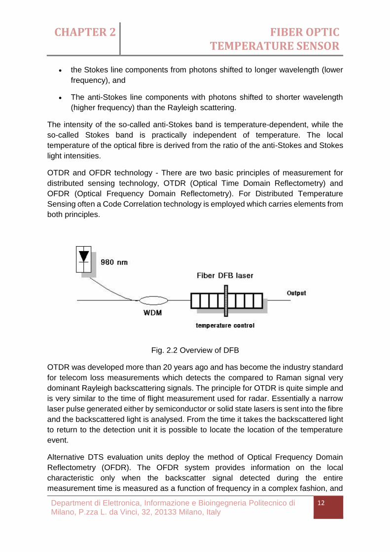
OTDR and OFDR technology - There are two basic principles of measurement for
distributed sensing technology, OTDR (Optical Time Domain Reflectometry) and
OFDR (Optical Frequency Domain Reflectometry). For Distributed Temperature
Sensing often a Code Correlation technology is employed which carries elements from
both principles.
Fig. 2.2 Overview of DFB
OTDR was developed more than 20 years ago and has become the industry standard
for telecom loss measurements which detects the compared to Raman signal very
dominant Rayleigh backscattering signals. The principle for OTDR is quite simple and
is very similar to the time of flight measurement used for radar. Essentially a narrow
laser pulse generated either by semiconductor or solid state lasers is sent into the fibre
and the backscattered light is analysed. From the time it takes the backscattered light
to return to the detection unit it is possible to locate the location of the temperature
event.
Alternative DTS evaluation units deploy the method of Optical Frequency Domain
Reflectometry (OFDR). The OFDR system provides information on the local
characteristic only when the backscatter signal detected during the entire
measurement time is measured as a function of frequency in a complex fashion, and
CHAPTER 2 FIBER OPTIC TEMPERATURE SENSOR
Department di Elettronica, Informazione e Bioingegneria Politecnico di Milano, P.zza L. da Vinci, 32, 20133 Milano, Italy
13
then subjected to Fourier transformation. The essential principles of OFDR technology
are the quasi continuous wave mode employed by the laser and the narrow-band
detection of the optical back scatter signal. This is offset by the technically difficult
measurement of the Raman scatter light and rather complex signal processing, due to
the FFT calculation with higher linearity requirements for the electronic components.
Code Correlation DTS sends on/off sequences of limited length into the fiber. The
codes are chosen to have suitable properties, e.g. Binary Golay code. In contrast to
OTDR technology, the optical energy is spread over a code rather than packed into a
single pulse. Thus a light source with lower peak power compared to OTDR
technology can be used, e.g. long life compact semiconductor lasers. The detected
backscatter needs to be transformed similar to OFDR technology back into a spatial
profile, e.g. by cross-correlation. In contrast to OFDR technology, the emission is finite
(for example 128 bits) which avoids that weak scattered signals from far are
superposed by strong scattered signals from short distance, improving the Shot noise
and the signal-to-noise ratio. Using these techniques it is possible to analyse distances
of greater than 30 km from one system and to measure temperature resolutions of
less than 0.01°C.
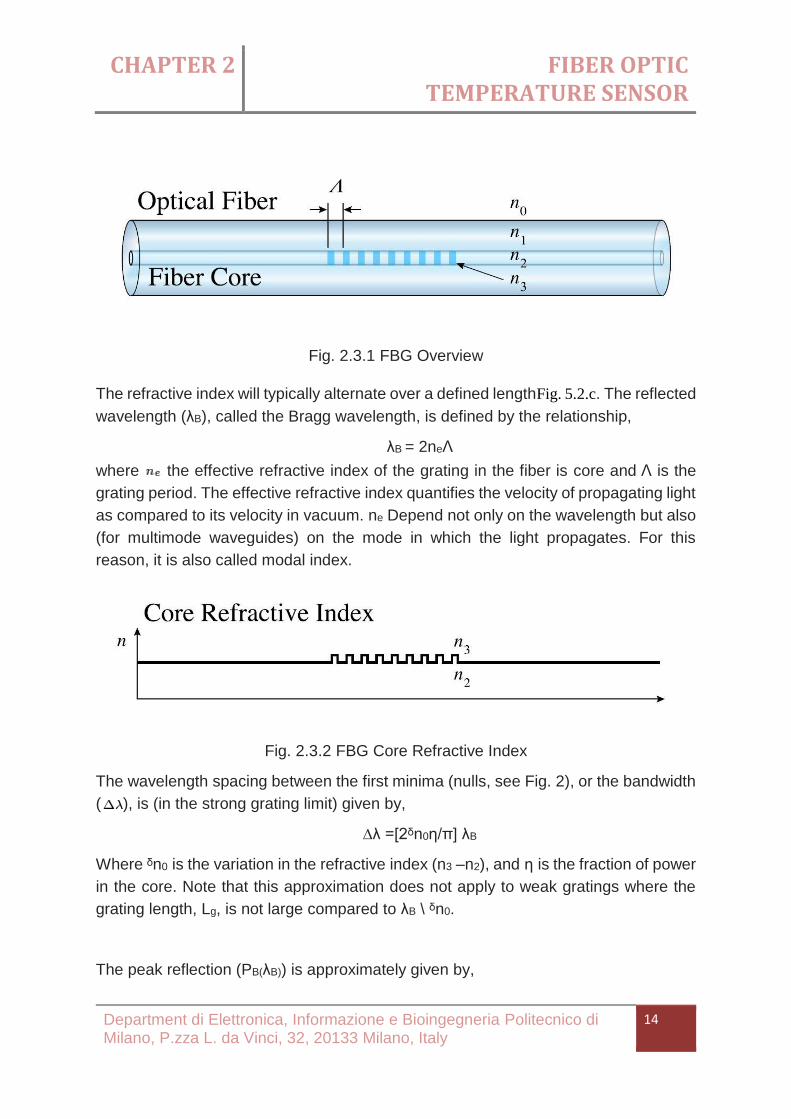
2.3 Fiber Bragg grating
A fiber Bragg grating (FBG) is a type of distributed Bragg reflector constructed
in a short segment of optical fiber that reflects particular wavelengths of light and
transmits all others. This is achieved by creating a periodic variation in the refractive
index of the fiber core, which generates a wavelength-specific dielectric mirror. A fiber
Bragg grating can therefore be used as an inline optical filter to block certain
wavelengths, or as a wavelength-specific reflector.
The fundamental principle behind the operation of a FBG is Fresnel reflection, where
light travelling between media of different refractive indices may
both reflect and refract at the interface.
CHAPTER 2 FIBER OPTIC TEMPERATURE SENSOR
Department di Elettronica, Informazione e Bioingegneria Politecnico di Milano, P.zza L. da Vinci, 32, 20133 Milano, Italy
14
Fig. 2.3.1 FBG Overview
The refractive index will typically alternate over a defined lengthFig. 5.2.c. The reflected
wavelength (λB), called the Bragg wavelength, is defined by the relationship,
λB = 2neΛ
where the effective refractive index of the grating in the fiber is core and Λ is the
grating period. The effective refractive index quantifies the velocity of propagating light
as compared to its velocity in vacuum. ne Depend not only on the wavelength but also
(for multimode waveguides) on the mode in which the light propagates. For this
reason, it is also called modal index.
Fig. 2.3.2 FBG Core Refractive Index
The wavelength spacing between the first minima (nulls, see Fig. 2), or the bandwidth
( ), is (in the strong grating limit) given by,
∆λ =[2ᵟn0η/π] λB
Where ᵟn0 is the variation in the refractive index (n3 –n2), and η is the fraction of power
in the core. Note that this approximation does not apply to weak gratings where the
grating length, Lg, is not large compared to λB \ ᵟn0.
The peak reflection (PB(λB)) is approximately given by,

CHAPTER 2 FIBER OPTIC TEMPERATURE SENSOR
Department di Elettronica, Informazione e Bioingegneria Politecnico di Milano, P.zza L. da Vinci, 32, 20133 Milano, Italy
15
where is the number of periodic variations. The full equation for the reflected power
( ), is given by,
where,
Fig. 2.3.3 FBG Spectral Response
2.4 Local Temperature Sensors
2.4.1 Fabry–Pérot Interferometer
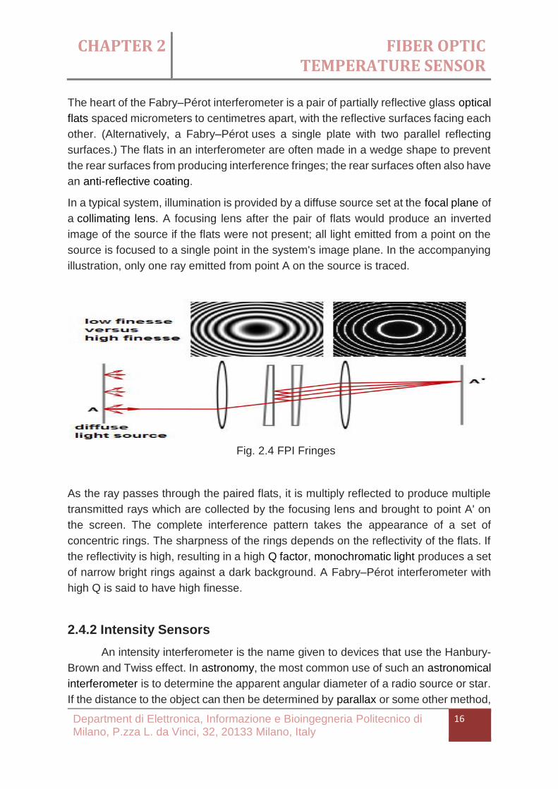
In optics, a Fabry–Pérot interferometer or etalon is typically made of a
transparent plate with two reflecting surfaces, or two parallel highly reflecting mirrors.
(Technically the former is an etalon and the latter is an interferometer, but the
terminology is often used inconsistently.) Its transmission spectrum as a function
of wavelength exhibits peaks of large transmission corresponding to resonances of
the etalon. It is named after Charles Fabry and Alfred Perot. "Etalon" is from the
French etalon, meaning "measuring gauge" or "standard".
Etalons are widely used in telecommunications, lasers and spectroscopy to control
and measure the wavelengths of light. Recent advances in fabrication technique allow
the creation of very precise tuneable Fabry–Pérot interferometers.
CHAPTER 2 FIBER OPTIC TEMPERATURE SENSOR
Department di Elettronica, Informazione e Bioingegneria Politecnico di Milano, P.zza L. da Vinci, 32, 20133 Milano, Italy
16
The heart of the Fabry–Pérot interferometer is a pair of partially reflective glass optical
flats spaced micrometers to centimetres apart, with the reflective surfaces facing each
other. (Alternatively, a Fabry–Pérot uses a single plate with two parallel reflecting
surfaces.) The flats in an interferometer are often made in a wedge shape to prevent
the rear surfaces from producing interference fringes; the rear surfaces often also have
an anti-reflective coating.
In a typical system, illumination is provided by a diffuse source set at the focal plane of
a collimating lens. A focusing lens after the pair of flats would produce an inverted
image of the source if the flats were not present; all light emitted from a point on the
source is focused to a single point in the system's image plane. In the accompanying
illustration, only one ray emitted from point A on the source is traced.
Fig. 2.4 FPI Fringes
As the ray passes through the paired flats, it is multiply reflected to produce multiple
transmitted rays which are collected by the focusing lens and brought to point A' on
the screen. The complete interference pattern takes the appearance of a set of
concentric rings. The sharpness of the rings depends on the reflectivity of the flats. If
the reflectivity is high, resulting in a high Q factor, monochromatic light produces a set
of narrow bright rings against a dark background. A Fabry–Pérot interferometer with
high Q is said to have high finesse.
2.4.2 Intensity Sensors
An intensity interferometer is the name given to devices that use the Hanbury-
Brown and Twiss effect. In astronomy, the most common use of such an astronomical
interferometer is to determine the apparent angular diameter of a radio source or star.
If the distance to the object can then be determined by parallax or some other method,

CHAPTER 2 FIBER OPTIC TEMPERATURE SENSOR
Department di Elettronica, Informazione e Bioingegneria Politecnico di Milano, P.zza L. da Vinci, 32, 20133 Milano, Italy
17
the physical diameter of the star can then be inferred. An example of an optical
intensity interferometer is the Narrabri Stellar Intensity Interferometer. In quantum
optics, some devices which take advantage of correlation and anti-correlation effects
in beams of photons might be said to be intensity interferometers, although the term
is usually reserved for observatories.
Either an intensity interferometer is built from two light detectors, typically radio
antenna or optical telescopes with photomultiplier tubes (PMTs), separated by some
distance, and called the baseline. Both detectors are pointed at the same astronomical
source, and intensity measurements are then transmitted to a central correlator facility.
A major advantage of intensity interferometers is that only the measured intensity
observed by each detector must be sent to the central correlator facility, rather than
the amplitude and phase of the signal. The intensity interferometer measures
interferometric visibilities like all other astronomical interferometers. These
measurements can be used to calculate the diameter and limb darkening coefficients
of stars, but with intensity interferometers aperture synthesis images cannot be
produced as the visibility phase information is not preserved by an intensity
interferometer.
The first fiber optic sensors were developed even before low-loss fibers became
available in the 1970s. They used bundles or single fibers to measure the light
reflected or transmitted by an object. This technology, which is elementary by today’s
standards, nevertheless provided the advantages of fiber optics to a limited number of
applications. As new fibers became available, the performance of sensors improved.
The availability of durable single-fiber cables allowed efficient optical systems and
miniature sensors to be employed. In addition to simple reflective and transmissive
systems, fringe tracking, micro bending, total reflection, and photo elastic techniques
were explored. Progress toward practical fiber optic sensors was rapid.
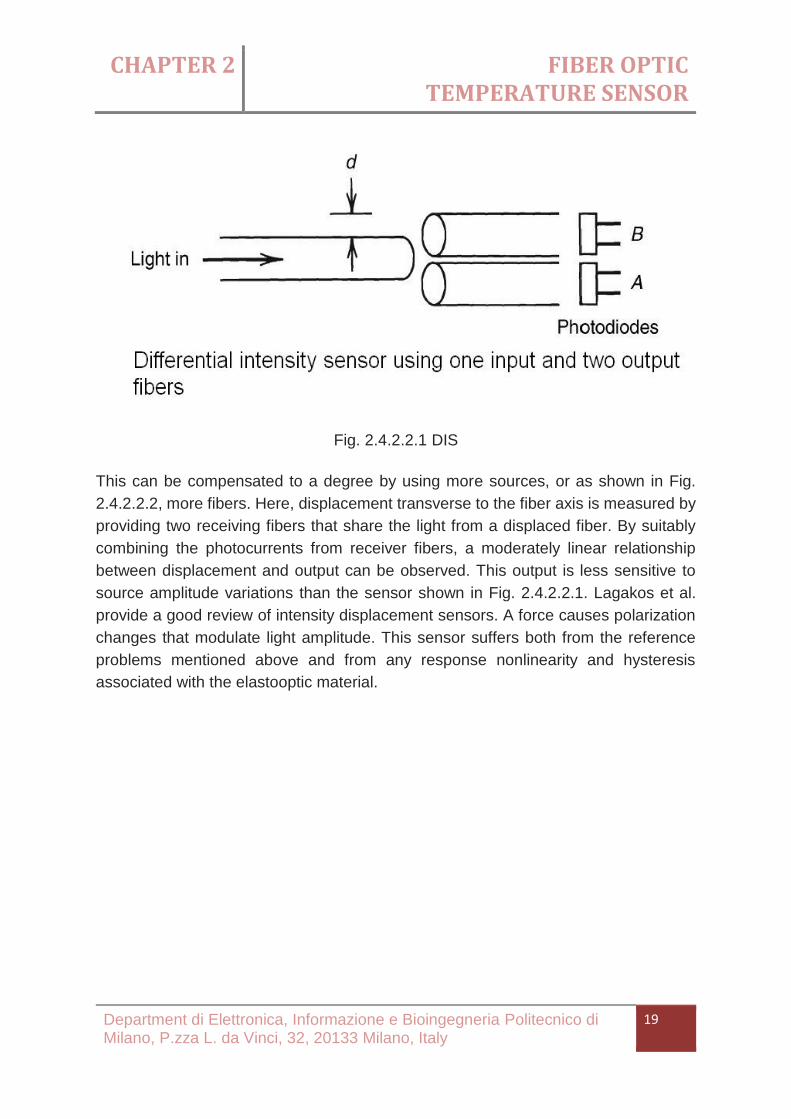
Intensity sensors are inherently simple and require only a modest amount of interface
electronics. Figure 2.4.2 shows how a single-fiber reflective sensor operates.

CHAPTER 2 FIBER OPTIC TEMPERATURE SENSOR
Department di Elettronica, Informazione e Bioingegneria Politecnico di Milano, P.zza L. da Vinci, 32, 20133 Milano, Italy
18
Fig. 2.4.2 Single Fiber Intensity Sensor
In this example, light travels along the fiber from left to right, leaves the fiber end in a
cone pattern, and strikes a movable reflector. If the reflector is close to the fiber end
(Fig. 2.4.2 a), most of the light is reflected back into the fiber; as the reflector moves
farther from the end of the fiber, as shown in Fig. 2.4.2 b and c, less light is coupled
back into the fiber. The monotonic relationship between fiber–reflector distance and
returned light can be used to determine distance. The obvious limitation of this sensor,
a limitation that is common to most intensity sensors, is lack of a suitable reference
signal. If the light source output level changes, or losses in the fiber vary with time, an
erroneous distance measurement will result.
CHAPTER 2 FIBER OPTIC TEMPERATURE SENSOR
Department di Elettronica, Informazione e Bioingegneria Politecnico di Milano, P.zza L. da Vinci, 32, 20133 Milano, Italy
19
Fig. 2.4.2.2.1 DIS
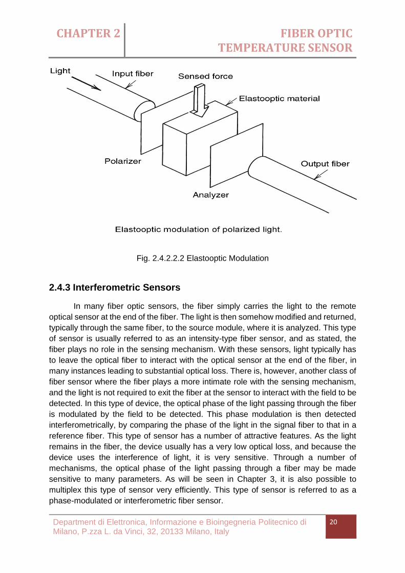
This can be compensated to a degree by using more sources, or as shown in Fig.
2.4.2.2.2, more fibers. Here, displacement transverse to the fiber axis is measured by
providing two receiving fibers that share the light from a displaced fiber. By suitably
combining the photocurrents from receiver fibers, a moderately linear relationship
between displacement and output can be observed. This output is less sensitive to
source amplitude variations than the sensor shown in Fig. 2.4.2.2.1. Lagakos et al.
provide a good review of intensity displacement sensors. A force causes polarization
changes that modulate light amplitude. This sensor suffers both from the reference
problems mentioned above and from any response nonlinearity and hysteresis
associated with the elastooptic material.
CHAPTER 2 FIBER OPTIC TEMPERATURE SENSOR
Department di Elettronica, Informazione e Bioingegneria Politecnico di Milano, P.zza L. da Vinci, 32, 20133 Milano, Italy
20
Fig. 2.4.2.2.2 Elastooptic Modulation
2.4.3 Interferometric Sensors
In many fiber optic sensors, the fiber simply carries the light to the remote
optical sensor at the end of the fiber. The light is then somehow modified and returned,
typically through the same fiber, to the source module, where it is analyzed. This type
of sensor is usually referred to as an intensity-type fiber sensor, and as stated, the
fiber plays no role in the sensing mechanism. With these sensors, light typically has
to leave the optical fiber to interact with the optical sensor at the end of the fiber, in
many instances leading to substantial optical loss. There is, however, another class of
fiber sensor where the fiber plays a more intimate role with the sensing mechanism,
and the light is not required to exit the fiber at the sensor to interact with the field to be
detected. In this type of device, the optical phase of the light passing through the fiber
is modulated by the field to be detected. This phase modulation is then detected
interferometrically, by comparing the phase of the light in the signal fiber to that in a
reference fiber. This type of sensor has a number of attractive features. As the light
remains in the fiber, the device usually has a very low optical loss, and because the
device uses the interference of light, it is very sensitive. Through a number of
mechanisms, the optical phase of the light passing through a fiber may be made
sensitive to many parameters. As will be seen in Chapter 3, it is also possible to
multiplex this type of sensor very efficiently. This type of sensor is referred to as a
phase-modulated or interferometric fiber sensor.

CHAPTER 2 FIBER OPTIC TEMPERATURE SENSOR
Department di Elettronica, Informazione e Bioingegneria Politecnico di Milano, P.zza L. da Vinci, 32, 20133 Milano, Italy
21
Fiber optic interferometric sensors, as well as having the advantages generally
attributed to fiber sensors, such as electrically passive (safety), lightweight, immunity
to electromagnetic interference (EMI), and multiplexing have the additional
advantages of geometric versatility of the sensing element, wide dynamic range, and
extremely high sensitivity. It is worthwhile to describe in greater etail the form of some
of these advantages. For an acoustic sensor, where approximately 30m of fiber is
required for the acoustic element, the fiber could be wrapped so as to form a small
golf-ball-sized omnidirectional hydrophone, or the element could be configured as a
highly directional element of 30m length—or any size between these two extremes.
As will be shown, fiber interferometric sensors can detect strains up to ~10-13 to 10-15;
this is the origin of their high sensitivity and wide dynamic range.
Consequently, there has been an intense research effort over the last 10 years to
develop sensors that capitalize on these advantages. However, it is some of these
“Advantages” that have tended to slow the progress of this very promising technology.
Fig. 2.4.3 Overview of Interferometric
For instance, the ability to make the fiber sensitive to many different parameters leads
to the problem of sensor selectivity. Acoustic sensors become accelerometers,
accelerometers become temperature sensors, and magnetometers become
seismometers, which for high-performance, state-of-the-art sensors is undesirable.
Another major difficulty is that while the relationship between the optical phase shift
and the parameter to be detected is linear over many orders of magnitude, the output
of the interferometer, owing to the “raised-cosine fringes,” requires processing, which
can limit dynamic range, degrade performance, and elevate the noise floor of the
system. The very high performance of the sensors also dictates stringent requirements
on the multiplexing of these sensors, so as to retain the system’s integrity with regard
to performance.
CHAPTER 3 COHERENT TEMPERATURE FIBER OPTIC SENSOR
Department di Elettronica, Informazione e Bioingegneria Politecnico di Milano, P.zza L. da Vinci, 32, 20133 Milano, Italy
22
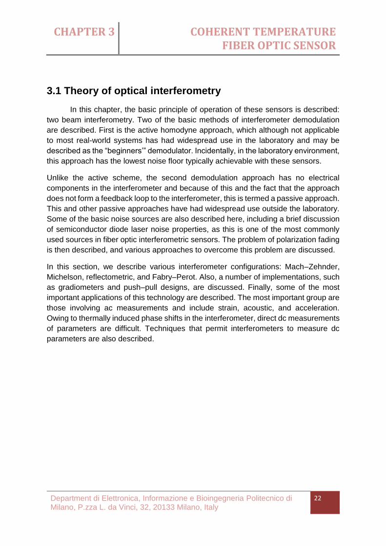
3.1 Theory of optical interferometry
In this chapter, the basic principle of operation of these sensors is described:
two beam interferometry. Two of the basic methods of interferometer demodulation
are described. First is the active homodyne approach, which although not applicable
to most real-world systems has had widespread use in the laboratory and may be
described as the “beginners’” demodulator. Incidentally, in the laboratory environment,
this approach has the lowest noise floor typically achievable with these sensors.
Unlike the active scheme, the second demodulation approach has no electrical
components in the interferometer and because of this and the fact that the approach
does not form a feedback loop to the interferometer, this is termed a passive approach.
This and other passive approaches have had widespread use outside the laboratory.
Some of the basic noise sources are also described here, including a brief discussion
of semiconductor diode laser noise properties, as this is one of the most commonly
used sources in fiber optic interferometric sensors. The problem of polarization fading
is then described, and various approaches to overcome this problem are discussed.
In this section, we describe various interferometer configurations: Mach–Zehnder,
Michelson, reflectometric, and Fabry–Perot. Also, a number of implementations, such
as gradiometers and push–pull designs, are discussed. Finally, some of the most
important applications of this technology are described. The most important group are
those involving ac measurements and include strain, acoustic, and acceleration.
Owing to thermally induced phase shifts in the interferometer, direct dc measurements
of parameters are difficult. Techniques that permit interferometers to measure dc
parameters are also described.

CHAPTER 3 COHERENT TEMPERATURE FIBER OPTIC SENSOR
Department di Elettronica, Informazione e Bioingegneria Politecnico di Milano, P.zza L. da Vinci, 32, 20133 Milano, Italy
23
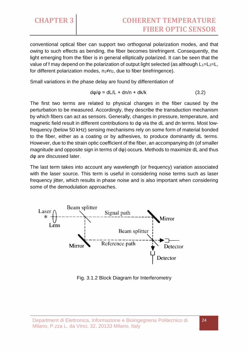
Fig. 3.1.1 Interference block diagram
Two-beam interferometry allows the measurement of extremely small
differential phase shifts in the optical fiber generated by the measurand. The optical
phase delay (in radians) of light passing through a fiber is given by
Φ=nkL (3.1)
where n is the refractive index of the fiber core, k is the optical wave number in vacuum
(2π/l, l being the wavelength), and L is the physical length of the fiber. It should be
noted that nL is referred to as the optical path length. It should also be noted that
CHAPTER 3 COHERENT TEMPERATURE FIBER OPTIC SENSOR
Department di Elettronica, Informazione e Bioingegneria Politecnico di Milano, P.zza L. da Vinci, 32, 20133 Milano, Italy
24
conventional optical fiber can support two orthogonal polarization modes, and that
owing to such effects as bending, the fiber becomes birefringent. Consequently, the
light emerging from the fiber is in general elliptically polarized. It can be seen that the
value of f may depend on the polarization of output light selected (as although L1=L2=L,
for different polarization modes, n1≠n2, due to fiber birefringence).
Small variations in the phase delay are found by differentiation of
dφ/φ = dL/L + dn/n + dk/k (3.2)
The first two terms are related to physical changes in the fiber caused by the
perturbation to be measured. Accordingly, they describe the transduction mechanism
by which fibers can act as sensors. Generally, changes in pressure, temperature, and
magnetic field result in different contributions to dφ via the dL and dn terms. Most low-
frequency (below 50 kHz) sensing mechanisms rely on some form of material bonded
to the fiber, either as a coating or by adhesives, to produce dominantly dL terms.
However, due to the strain optic coefficient of the fiber, an accompanying dn (of smaller
magnitude and opposite sign in terms of dφ) occurs. Methods to maximize dL and thus
dφ are discussed later.
The last term takes into account any wavelength (or frequency) variation associated
with the laser source. This term is useful in considering noise terms such as laser
frequency jitter, which results in phase noise and is also important when considering
some of the demodulation approaches.
Fig. 3.1.2 Block Diagram for Interferometry
CHAPTER 3 COHERENT TEMPERATURE FIBER OPTIC SENSOR
Department di Elettronica, Informazione e Bioingegneria Politecnico di Milano, P.zza L. da Vinci, 32, 20133 Milano, Italy
25
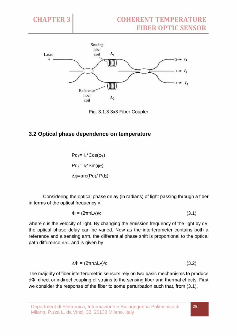
Fig. 3.1.3 3x3 Fiber Coupler
3.2 Optical phase dependence on temperature
Pd1= I1*Cos(φ1)
Pd2= I2*Sin(φ2)
∆φ=arc(Pd1/ Pd2)
Considering the optical phase delay (in radians) of light passing through a fiber
in terms of the optical frequency ν,
Φ = (2πnLν)/c (3.1)
where c is the velocity of light. By changing the emission frequency of the light by dν,
the optical phase delay can be varied. Now as the interferometer contains both a
reference and a sensing arm, the differential phase shift is proportional to the optical
path difference n∆L and is given by
∆Φ = (2πn∆Lν)/c (3.2)
The majority of fiber interferometric sensors rely on two basic mechanisms to produce
dΦ: direct or indirect coupling of strains to the sensing fiber and thermal effects. First
we consider the response of the fiber to some perturbation such that, from (3.1),
CHAPTER 3 COHERENT TEMPERATURE FIBER OPTIC SENSOR
Department di Elettronica, Informazione e Bioingegneria Politecnico di Milano, P.zza L. da Vinci, 32, 20133 Milano, Italy
26
Φ = (2πnLν)/c
∆Φ = kd(nL) = k(ndL + Ldn) (3.3)
∆Φ = kL(ndL/L + dn) (3.4)
where n dL corresponds to a physical change in length and L dn to changes in the
refractive index. Dependent on the mechanism of the response either the n dL or the
L dn term may dominate. dL/L is the fiber strain. It may be shown that the phase
response of the fiber to axial strain is given by
dΦ = kξndL (3.5)
where ξ is the strain optic correction factor and is given by 1-n2[(1-μ)p12- μp11]/2, μ is
the Poisson’s ratio, and pij are the elements of the strain optic tensor (Pockel’s
coefficients) of the fiber. Typically, ξ has a value of ~0.78 in silica glass fibers. Thus,
the length change in the fiber plays the major role in strain sensing.
If we now consider the response of the fiber to temperature, from Eq. (3.3),
dΦ/dT = k(n(dL/dT) + L(dn/dT)) (3.6)
for a typical silica fiber dL/(LdT)= 5x10⁻⁷ K-1 and dn/dT=1x10-5 K-1 such that clearly the
refractive index term dominates (dΦ~100 rad/(m K)). If, however, we consider the case
of a silica fiber with a 1mm diameter nylon jacket, dL/(LdT) for the composite structure
is now ~6.5x10⁻⁵ K-1 such that now the thermally induced length change dominates the
optical phase shift.
As mentioned earlier, two-beam interferometric fiber sensors of the Michelson
and Mach–Zehnder types exhibit extremely high sensitivity to temperature and
arrange of other measurand fields that can be transformed into strain in an optical fiber
(i.e., pressure, acceleration, displacement, etc.). Unfortunately, the output of an
interferometric fiber sensor is intrinsically ambiguous due to the periodic nature of the
raised-cosine transfer function. Therefore, when dc measurands are of interest, the
absolute value of the measurand cannot be determined when the sensor is initialized.
A number of approaches to overcoming this ambiguity problem have been proposed

CHAPTER 3 COHERENT TEMPERATURE FIBER OPTIC SENSOR
Department di Elettronica, Informazione e Bioingegneria Politecnico di Milano, P.zza L. da Vinci, 32, 20133 Milano, Italy
27
and demonstrated: (1) two-wavelength interrogation (2) combined
interferometric/polarimetric configurations, and (3) nonlinear phase transduction
mechanisms.
Dual-wavelength interrogation of the sensor can be used to circumvent the ambiguity
limitation of the interferometric sensing approach if the upper and lower bounds of the
sensor range are well defined. The principle of the approach is as follows. Using a
demodulation technique based on determination of the interferometric phase
excursion at two wavelengths, the unambiguous range of a basic interferometric
sensor can be increased substantially. The difference in the phase shift measured at
each wavelength (λ1, λ2) is a function of the interferometer path difference and displays
unambiguous range (±π), which, depending on the actual wavelength difference used,
can correspond to more than ±100 individual interferometer fringes. Operation of the
sensor within this range allows absolute determination of the measurand field (e.g.,
temperature) on initialization.
For an interferometer of path imbalance DL illuminated by two coherent sources of
wavelength (frequency) λ1(v1) and λ2(v2), the phase differences between the arms of
the interferometer at each wavelength are
∆Φ1(λ1) = (2πn∆L)/λ1 = (2πn∆Lν1)/c (3.7a)
∆Φ2(λ2) = (2πn∆L)/λ2 = (2πn∆Lν2)/c (3.7b)
where n is the core effective index (we assume Dl is small so that dispersion can be
neglected) and c is the free-space velocity of light. The relative phase difference is
thus
∆Φ = (2πn∆L(ν1-v2))/c (3.8)

CHAPTER 3 COHERENT TEMPERATURE FIBER OPTIC SENSOR
Department di Elettronica, Informazione e Bioingegneria Politecnico di Milano, P.zza L. da Vinci, 32, 20133 Milano, Italy
28
Fig. 3.2 Output response for interferometric
The unambiguous range in ∆L is determined by -π<∆φ<π. However, if DL consists of
a finite path mismatch ∆L plus a measurand induced change dL, where ∆L’ is much
greater than the maximum dL, the determination of dL through the measurement of
∆L will depend critically on the stability of the laser frequencies. The wavelength
instabilities become important only when the sensor output ∆φ is approaching -π
radians.

CHAPTER 4 CHIRP MODULATION
Department di Elettronica, Informazione e Bioingegneria Politecnico di Milano, P.zza L. da Vinci, 32, 20133 Milano, Italy
29
4.1 LASER CHIRP MODULATION
A chirp is a signal in which the frequency increases or decreases with time. In some
sources, the term chirp is used interchangeably with sweep signal. It is commonly used in
sonar and radar, but has other applications, such as in spread spectrum communications. In
spread spectrum usage, SAW devices such as RACs are often used to generate and
demodulate the chirped signals. In optics, ultra short laser pulses also exhibit chirp, which, in
optical transmission systems interacts with the dispersion properties of the materials,
increasing or decreasing total pulse dispersion as the signal propagates.
4.1.1 Linear chirp
In a linear chirp, the instantaneous frequency varies linearly with time:
where is the starting frequency (at time ), and is the rate of frequency
increase or chirp rate.
where is the final frequency and is the starting frequency. is the time it takes
to sweep from to .
The corresponding time-domain function for the phase of any oscillating signal is the
integral of the frequency function, since one expects the phase to grow
like , i.e., that the derivative of the phase is the
angular frequency .
For the linear chirp, this results in:

CHAPTER 4 CHIRP MODULATION
Department di Elettronica, Informazione e Bioingegneria Politecnico di Milano, P.zza L. da Vinci, 32, 20133 Milano, Italy
30
where is the initial phase (at time ). Thus this is also called quadratic-phase
signal.
The corresponding time-domain function for a sinusoidal linear chirp is the sine of the
phase in radians:
In the frequency domain, the instantaneous frequency described by the
equation is accompanied by additional frequencies (harmonics)
which exist as a fundamental consequence of frequency modulation. These
harmonics are quantifiably described through the use of Bessel functions. However,
with the aid of a frequency vs. time profile spectrogram one can readily see that the
linear chirp has spectral components at harmonics of the fundamental chirp.
4.1.2 Exponential chirp
In a geometric chirp, also called an exponential chirp, the frequency of the
signal varies with a geometric relationship over time. In other words, if two points in
the waveform are chosen, and , and the time interval between them is
kept constant, the frequency ratio will also be constant.
In an exponential chirp, the frequency of the signal varies exponentially as a function
of time:
where is the starting frequency (at ), and is the rate of exponential
increase in frequency. Unlike the linear chirp, which has a constant chirp rate, an
exponential chirp has an exponentially increasing chirp rate.

CHAPTER 4 CHIRP MODULATION
Department di Elettronica, Informazione e Bioingegneria Politecnico di Milano, P.zza L. da Vinci, 32, 20133 Milano, Italy
31
The corresponding time-domain function for the phase of an exponential chirp is the
integral of the frequency:
Where is the initial phase (at ).
The corresponding time-domain function for a sinusoidal exponential chirp is the sine
of the phase in radians:
As was the case for the Linear Chirp, the instantaneous frequency of the Exponential
Chirp consists of the fundamental frequency accompanied by
additional harmonics.
4.2 LASER DIODES
A laser diode, or LD, is an electrically pumped semiconductor laser in which the
active laser medium is formed by a p-n junction of a semiconductor diode similar to
that found in a light-emitting diode.
The laser diode is the most common type of laser produced with a wide range of uses
that include fiber optic communications, barcode readers, laser pointers, CD/DVD/Blu-
ray Disc reading and recording, laser printing, laser scanning and increasingly
directional lighting sources.
CHAPTER 4 CHIRP MODULATION
Department di Elettronica, Informazione e Bioingegneria Politecnico di Milano, P.zza L. da Vinci, 32, 20133 Milano, Italy
32
4.2.1 Operation
A laser diode is electrically a P-i-n diode. The active region of the laser diode is in the
intrinsic (I) region and the carriers (electrons and holes) are pumped into that region
from the N and P regions respectively. While initial diode laser research was
conducted on simple P-N diodes, all modern lasers use the double-hetero structure
implementation, where the carriers and the photons are confined in order to maximize
their chances for recombination and light generation. Unlike a regular diode, the goal
for a laser diode is to recombine all carriers in the I region, and produce light. Thus,
laser diodes are fabricated using direct band-gap semiconductors. The laser diode
epitaxial structure is grown using one of the crystal growth techniques, usually starting
from an N doped substrate, and growing the I doped active layer, followed by the P
doped cladding, and a contact layer. The active layer most often consists of quantum
wells, which provide lower threshold current and higher efficiency.[1]
Laser diodes form a subset of the larger classification of semiconductor p-n junction
diodes. Forward electrical bias across the laser diode causes the two species of
charge carrier – holes and electrons – to be "injected" from opposite sides of the p-n
junction into the depletion region. Holes are injected from the p-doped, and electrons
from the n-doped, semiconductor. (A depletion region, devoid of any charge carriers,
forms as a result of the difference in electrical potential between n- and p-type
semiconductors wherever they are in physical contact.) Due to the use of charge
injection in powering most diode lasers, this class of lasers is sometimes termed
"injection lasers “or” injection laser diode" (ILD). As diode lasers are semiconductor
devices, they may also be classified as semiconductor lasers. Either designation
distinguishes diode lasers from solid-state lasers.
4.2.2 Different type of laser diode
The simple laser diode structure, described above, is extremely inefficient. Such
devices require so much power that they can only achieve pulsed operation without
damage. Although historically important and easy to explain, such devices are not
practical.
CHAPTER 4 CHIRP MODULATION
Department di Elettronica, Informazione e Bioingegneria Politecnico di Milano, P.zza L. da Vinci, 32, 20133 Milano, Italy
33
4.2.2.1 VCSEL
The vertical-cavity surface-emitting laser, or VCSEL, is a type of semiconductor
laser diode with laser beam emission perpendicular from the top surface, contrary to
conventional edge-emitting semiconductor lasers (also in-plane lasers) which emit
from surfaces formed by cleaving the individual chip out of a wafer.
There are several advantages to producing VCSELs, in contrast to the production
process of edge-emitting lasers. Edge-emitters cannot be tested until the end of the
production process. If the edge-emitter does not function properly, whether due to bad
contacts or poor material growth quality, the production time and the processing
materials have been wasted. VCSELs however, can be tested at several stages
throughout the process to check for material quality and processing issues. For
instance, if the vias have not been completely cleared of dielectric material during the
etch, an interim testing process will flag that the top metal layer is not making contact
to the initial metal layer. Additionally, because VCSELs emit the beam perpendicular
to the active region of the laser as opposed to parallel as with an edge emitter, tens of
thousands of VCSELs can be processed simultaneously on a three inch Gallium
Arsenide wafer. Furthermore, even though the VCSEL production process is more
labor and material intensive, the yield can be controlled to a more predictable outcome.
4.2.2.1.1 Structure
The laser resonator consists of two distributed Bragg reflector (DBR) mirrors
parallel to the wafer surface with an active region consisting of one or more quantum
wells for the laser light generation in between. The planar DBR-mirrors consist of
layers with alternating high and low refractive indices. Each layer has a thickness of a
quarter of the laser wavelength in the material, yielding intensity reflectivities above
99%. High reflectivity mirrors are required in VCSELs to balance the short axial length
of the gain region.
In common VCSELs the upper and lower mirrors are doped as p-type and n-type
materials, forming a diode junction. In more complex structures, the p-type and n-type
regions may be embedded between the mirrors, requiring a more complex
semiconductor process to make electrical contact to the active region, but eliminating
electrical power loss in the DBR structure.
In laboratory investigation of VCSELs using new material systems, the active region
may be pumped by an external light source with a shorter wavelength, usually another
laser. This allows a VCSEL to be demonstrated without the additional problem of

CHAPTER 4 CHIRP MODULATION
Department di Elettronica, Informazione e Bioingegneria Politecnico di Milano, P.zza L. da Vinci, 32, 20133 Milano, Italy
34
achieving good electrical performance; however such devices are not practical for
most applications.
VCSELs for wavelengths from 650 nm to 1300 nm are typically based on gallium
arsenide (GaAs) wafers with DBRs formed from GaAs and aluminium gallium arsenide
(AlxGa (1-x) As). The GaAs–AlGaAs system is favored for constructing VCSELs
because the lattice constant of the material does not very strongly as the composition
is changed, permitting multiple "lattice-matched" epitaxial layers to be grown on a
GaAs substrate. However, the refractive index of AlGaAs does vary relatively strongly
as the Al fraction is increased, minimizing the number of layers required to form an
efficient Bragg mirror compared to other candidate material systems. Furthermore, at
high aluminium concentrations, an oxide can be formed from AlGaAs, and this oxide
can be used to restrict the current in a VCSEL, enabling very low threshold currents.
Recently the two main methods of restricting the current in a VCSEL were
characterized by two types of VCSELs: ion-implanted VCSELs and Oxide VCSELs.
In the early 1990s, telecommunications companies tended to favor ion-implanted
VCSELs. Ions, (often hydrogen ions, H+), were implanted into the VCSEL structure
everywhere except the aperture of the VCSEL, destroying the lattice structure around
the aperture, thus inhibiting the current. In the mid to late 1990s, companies moved
towards the technology of oxide VCSELs. The current is confined in an oxide VCSEL
by oxidizing the material around the aperture of the VCSEL. A high content aluminium
layer that is grown within the VCSEL structure is the layer that is oxidized. Oxide
VCSELs also often employ the ion implant production step. As a result in the oxide
VCSEL, the current path is confined by the ion implant and the oxide aperture.
The initial acceptance of oxide VCSELs was plagued with concern about the apertures
"popping off" due to the strain and defects of the oxidation layer. However, after much
testing, the reliability of the structure has proven to be robust. As stated in one study
by Hewlett Packard on oxide VCSELs, "The stress results show that the activation
energy and the wear-out lifetime of oxide VCSEL are similar to that of implant VCSEL
emitting the same amount of output power."
A production concern also plagued the industry when moving the oxide VCSELs from
research and development to production mode. The oxidation rate of the oxide layer
was highly dependent on the aluminium content. Any slight variation in aluminium
would change the oxidation rate sometimes resulting in apertures that were either too
big or too small to meet the specification standards.
Longer wavelength devices, from 1300 nm to 2000 nm, have been demonstrated with
at least the active region made of indium phosphate. VCSELs at even higher
wavelengths are experimental and usually optically pumped. 1310 nm VCSELs are
CHAPTER 4 CHIRP MODULATION
Department di Elettronica, Informazione e Bioingegneria Politecnico di Milano, P.zza L. da Vinci, 32, 20133 Milano, Italy
35
desirable as the dispersion of silica-based optical fiber is minimal in this wavelength
range.
4.2.2.1.2 Characteristic
Multiple active region devices (aka bipolar cascade VCSELs). Allows for
differential quantum efficiency values in excess of 100% through carrier
recycling.
VCSELs with tunnel junctions. Using a tunnel junction (n+p+), an electrically
advantageous n-n+p+-p-i-n configuration can be built that also may beneficially
influence other structural elements (e.g. in the form of a Buried Tunnel Junction
(BTJ)).
Widely tuneable VCSELs with micromechanically (MEMS) movable mirrors
(either optically [1] or electrically pumped [2])
Wafer-bonded or wafer-fused VCSEL: Combination of semiconductor materials
that can be fabricated using different types of substrate wafers.
Monolithically optically pumped VCSELs: Two VCSELs on top of each other.
One of them optically pumps the other one.
VCSEL with longitudinally integrated monitor diode: A photodiode is integrated
under the back mirror of the VCSEL.
VCSEL with transversally integrated monitor diode: With suitable etching of the
VCSEL's wafer, a resonant photodiode can be manufactured that may measure
the light intensity of a neighbouring VCSEL.
VCSELs with external cavities, known as VECSELs or semiconductor disk
lasers. VECSELs are optically pumped with conventional laser diodes. This
arrangement allows a larger area of the device to be pumped and therefore
more power can be extracted - as much as 30W. The external cavity also allows
intracavity techniques such as frequency doubling, single frequency operation
and femtosecond pulse mode locking.
Vertical-cavity semiconductor optical amplifiers, known as VCSOAs. These
devices are optimized as amplifiers as opposed to oscillators. VCSOAs must
be operated below threshold and thus require reduced mirror reflectivities for
decreased feedback. In order to maximize the signal gain, these devices
contain a large number of quantum wells (optically pumped devices have been
demonstrated with 21–28 wells) and as a result exhibit single-pass gain values
which are significantly larger than that of a typical VCSEL (roughly 5%). These
structures operate as narrow line width (tens of GHz) amplifiers and may be
implemented as amplifying filters.

CHAPTER 4 CHIRP MODULATION
Department di Elettronica, Informazione e Bioingegneria Politecnico di Milano, P.zza L. da Vinci, 32, 20133 Milano, Italy
36
Because VCSELs emit from the top surface of the chip, they can be tested on-
wafer, before they are cleaved into individual devices. This reduces the fabrication
cost of the devices. It also allows VCSELs to be built not only in one-dimensional, but
also in two-dimensional arrays.
The larger output aperture of VCSELs, compared to most edge-emitting lasers,
produces a lower divergence angle of the output beam, and makes possible high
coupling efficiency with optical fibers.
The high reflectivity mirrors, compared to most edge-emitting lasers, reduce the
threshold current of VCSELs, resulting in low power consumption. However, as yet,
VCSELs have lower emission power compared to edge-emitting lasers. The low
threshold current also permits high intrinsic modulation bandwidths in VCSELs.
The wavelength of VCSELs may be tuned, within the gain band of the active region,
by adjusting the thickness of the reflector layers.
While early VCSELs emitted in multiple longitudinal modes or in filament modes,
single-mode VCSELs are now common.
4.2.2.2 Distributed feedback laser
A distributed feedback laser (DFB) is a type of laser diode, quantum cascade
laser or optical fiber laser where the active region of the device is periodically
structured as a diffraction grating. The structure builds a one-dimensional interference
grating (Bragg scattering) and the grating provides optical feedback for the laser.
DFB laser diodes do not use two discrete mirrors to form the optical cavity (as they
are used in conventional laser designs). The grating acts as the wavelength selective
element for at least one of the mirrors and provides the feedback, reflecting light back
into the cavity to form the resonator. The grating is constructed so as to reflect only a
narrow band of wavelengths, and thus produce a single longitudinal lasing mode. This
is in contrast to a Fabry-Perot Laser, where the facets of the chip form the two mirrors
and provide the feedback. In that case, the mirrors are broadband and either the laser
functions at multiple longitudinal modes simultaneously or easily jump between
longitudinal modes. Altering the temperature of the device causes the pitch of the
grating to change due to the dependence of refractive index on temperature. This
dependence is caused by a change in the semiconductor laser's band gap with
temperature and thermal expansion. A change in the refractive index alters the
wavelength selection of the grating structure and thus the wavelength of the laser
output, producing a wavelength tunable laser or TDL (Tunable Diode Laser). The
tuning range is usually of the order of 6 nm for a ~50 K (90 °F) change in temperature,

CHAPTER 4 CHIRP MODULATION
Department di Elettronica, Informazione e Bioingegneria Politecnico di Milano, P.zza L. da Vinci, 32, 20133 Milano, Italy
37
while the line width of a DFB laser is a few megahertz. Altering of the current powering
the laser will also tune the device, as a current change causes a temperature change
inside the device. Integrated DFB lasers are often used in optical communication
applications, such as DWDM where a tunable laser signal is desired as well as in
sensing where extreme narrow line width is required, or in gas sensing applications,
where the signal of the absorbing gas is detected while wavelength tuning the DFB
laser.
There are alternatives to traditional types of DFB lasers. Traditionally, DFBs are
antireflection coated on one side of the cavity and coated for high reflectivity on the
other side (AR/HR). In this case the grating forms the distributed mirror on the
antireflection coated side, while the semiconductor facet on the high reflectivity side
forms the other mirror. These lasers generally have higher output power since the light
is taken from the AR side, and the HR side prevents power being lost from the back
side. Unfortunately, during the manufacturing of the laser and the cleaving of the
facets, it is virtually impossible to control at which point in the grating the laser cleaves
to form the facet. So sometimes the laser HR facet forms at the crest of the grating,
sometimes on the slope. Depending on the phase of the grating and the optical mode,
the laser output spectrum can vary. Frequently, the phase of the highly reflective side
occurs at a point where two longitudinal modes have the same cavity gain, and thus
the laser operates at two modes simultaneously. Thus such AR/HR lasers have to be
screened at manufacturing and parts that are multimode or have poor side mode
suppression ratio (SMSR) have to be scrapped. Additionally, the phase of the cleave
affects the wavelength, and thus controlling the output wavelength of a batch of lasers
in manufacturing can be a challenge.
An alternative approach is a phase-shifted DFB laser. In this case both facets are anti-
reflection coated and there is a phase shift in the cavity. This could be a single 1/4
wave shift at the center of the cavity, or multiple smaller shifts distributed in the cavity.
Such devices have much better reproducibility in wavelength and theoretically all
lasers in single mode.
In DFB fibre lasers the Bragg grating (which in this case forms also the cavity of the
laser) has a phase-shift centered in the reflection band akin to a single very narrow
transmission notch of a Fabry–Pérot interferometer. When configured properly, these
lasers operate on a single longitudinal mode with coherence lengths in excess of tens
of kilometres, essentially limited by the temporal noise induced by the self-heterodyne
coherence detection technique used to measure the coherence. These DFB fibre
lasers are often used in sensing applications where extreme narrow line width is
required.
When we want to use lasers for long distance communication we find that standard
FP lasers have significant problems:

CHAPTER 4 CHIRP MODULATION
Department di Elettronica, Informazione e Bioingegneria Politecnico di Milano, P.zza L. da Vinci, 32, 20133 Milano, Italy
38
1. As seen above FP lasers produce many wavelengths over a spectral width of
between 5 and 8 nm. Even if we are using the 1310 “zero dispersion” band or
“dispersion shifted” fibre in the 1550 nm band there will still be some chromatic
dispersion of the signal caused by dispersion being slightly different at the different
wavelengths.
2. The “mode hopping” behaviour of FP lasers gives rise to “Mode Partition Noise” as
described in 2.4.3, “Mode Partition Noise”.
3. In Wavelength Division Multiplexed (WDM) systems we want to carry many
multiplexed optical signals on the same fibre. To do this it is important for each signal
to have as narrow a spectral width as possible and to be as stable as possible. Regular
FP lasers have too great a spectral width for use in this application.
Distributed Feedback (DFB) lasers are one answer to this problem. The idea is that
you put a Bragg grating into the laser cavity of an index-guided FP laser. This is just a
periodic variation in the RI of the gain region along its length.52 the presence of the
grating causes small reflections to occur at each RI change (corrugation). When the
period of the corrugations is a multiple of the wavelength of the incident light,
constructive interference between reflections occurs and a proportion of the light is
reflected. Other wavelengths destructively interfere and therefore cannot be reflected.
The effect is strongest when the period of the Bragg grating is equal to the wavelength
of light used (first order grating). However, the device will work when the grating period
is any (small) integer multiple of the wavelength. Thus only one mode (the one that
conforms to the wavelength of the grating) can lase.
Fig.4.2.2.2.1 DFB Active Region
Early devices using this principle had the grating within the active region and were
found to have too much attenuation. As a result the grating was moved to a waveguide
layer immediately adjacent to (below) the cavity. The evanescent field accompanying
the light wave in the cavity extends into the adjacent layer and interacts with the grating
to produce the desired effect.
In principle a DFB laser doesn’t need end mirrors. The grating can be made strong
enough to produce sufficient feedback (reflection) for lasing to take place. However,
in a perfect DFB laser there are actually two lines produced (one at each side of the

CHAPTER 4 CHIRP MODULATION
Department di Elettronica, Informazione e Bioingegneria Politecnico di Milano, P.zza L. da Vinci, 32, 20133 Milano, Italy
39
Bragg wavelength). We only want one line. A way of achieving this and improving the
efficiency of the device is to place a high reflectance end mirror at one end of the cavity
and either an AR coating or just a cleaved facet at the output end. In this case the
grating doesn’t need to be very strong - just sufficient to ensure that a single mode
dominates. The added reflections (from the end mirrors) act to make the device
asymmetric and suppress one of the two spectral lines. Unfortunately they also act to
increase the line width.
A schematic view of a DFB laser is shown in Figure DFB1. DFB lasers are very
effective and widely used but they have a problem with chirp. There are two main
sources of chirp:
1. When the current is switched on the charge carrier (electron and hole) flux in the
cavity changes very rapidly. This causes a change in the refractive index. A change in
refractive index (of course) changes the resonant wavelength of the grating and the
wavelength of the laser output changes (typically the wavelength gets longer) in well
less than a single bit time.
2. During lasing the cavity heats up. This also happens very quickly (in a lot less than
a bit time). This heating has two principal effects:
a. It causes the RI of the cavity to change.
b. It changes the electron energy gap in the material.
In an FP laser (as distinct from a DBR or DFB laser) this change in the energy gap
dominates other effects and is the predominant cause of chirp. In the DFB laser the
energy gap change is irrelevant. This is because the energy gap covers a range of
energies and the DFB resonant wavelength is determined by the grating spacing and
the cavity RI. So long as the range of energies in the gap extends to cover the resonant
wavelength then the device will lase.
This means that a DFB laser will chirp far less than an FP laser. This is because chirp
in DFB lasers is caused by the effect of the change in RI. This effect is much smaller
than the effect caused by the change in the energy gap (which dominates in FP lasers
but doesn’t affect DFBs).

CHAPTER 4 CHIRP MODULATION
Department di Elettronica, Informazione e Bioingegneria Politecnico di Milano, P.zza L. da Vinci, 32, 20133 Milano, Italy
40
Fig. 4.2.2.2.2 DFB Region
Sometimes DFB lasers are constructed with a quarter-wave phase shift in the middle
section of the grating as shown in Figure DFB2. This phase shift introduces a sharp
transmission “fringe” into the grating reflection band. The fringe acts to narrow the line
width of the laser significantly.
Fig. 4.2.2.2.3 DFB Response
Figure DFB3 shows the reflective characteristics of an un-shifted and a shifted Bragg
grating structure. Ascending values on the y-axis represent increasing percentage of
reflection. The x-axis represents wavelength. The axes have not been scaled because
the numerical values depend on the period and strength of the grating itself. The phase
shifted case (on the right of the figure) shows that a narrow pass band exists in the
middle of the reflection band. This is caused by the quarter-wave phase shift. What
happens is that the reflected waves from each end of the grating will be out of phase
with each other and hence will destructively interfere.
DFB lasers have a number of significant advantages over FP types:
1. They can exhibit very narrow line widths (of the order of 50 kHz).
2. They have quite low chirp as discussed above.
3. They typically have a very low Relative Intensity Noise (RIN).

CHAPTER 4 CHIRP MODULATION
Department di Elettronica, Informazione e Bioingegneria Politecnico di Milano, P.zza L. da Vinci, 32, 20133 Milano, Italy
41
Nothing however is completely without problems:
1. DBR lasers are extremely sensitive to reflections.
Any reflection entering the cavity will disturb the laser’s stable resonance. This causes
a widening of the line width. To the extent that reflections returning from the outside
vary (see 2.4.4, “Reflections and Return Loss Variation” on page 67) this can also be
a significant source of noise. To minimise the effects of this problem DFB lasers are
often packaged with an isolator integrated within the assembly. However, these don’t
always suppress all reflections and additional steps must be taken in system design
to minimise the problem.
2. They are sensitive to temperature variations in two ways:
a. The stable (average) temperature of the device has a very strong influence on
wavelength. Wavelength variation on a scale of many seconds or longer doesn’t have
much detrimental effect on a single channel long distance communication system but
it is a critical issue in WDM systems.
The device requires temperature control for stable operation. This is usually provided
by including a “Peltier Effect” cooler in the laser package.
b. During transmission (in even one bit time) the cavity heats up. If a long series of “1”
bits are transmitted this can cause a significant wavelength shift on a time scale too
short to be compensated by the Peltier cooler. This introduces a requirement that
higher layer link protocols be “balanced” and spend (on average) as much time in the
“0” state as in the “1” state.
3. Varying conditions produce significant fluctuations in laser output power. This is
undesirable for many reasons. To counter this PIN diode is often included in the laser
package near the “back facet”. This diode picks up a small proportion of generated
light from the transmittance of the back facet and provides input to a feedback loop for
control of laser drive current.
4. They have a relatively high cost. As seen above, to get stable operation you almost
always need temperature control, power control and optical isolation. All this adds to
the cost.
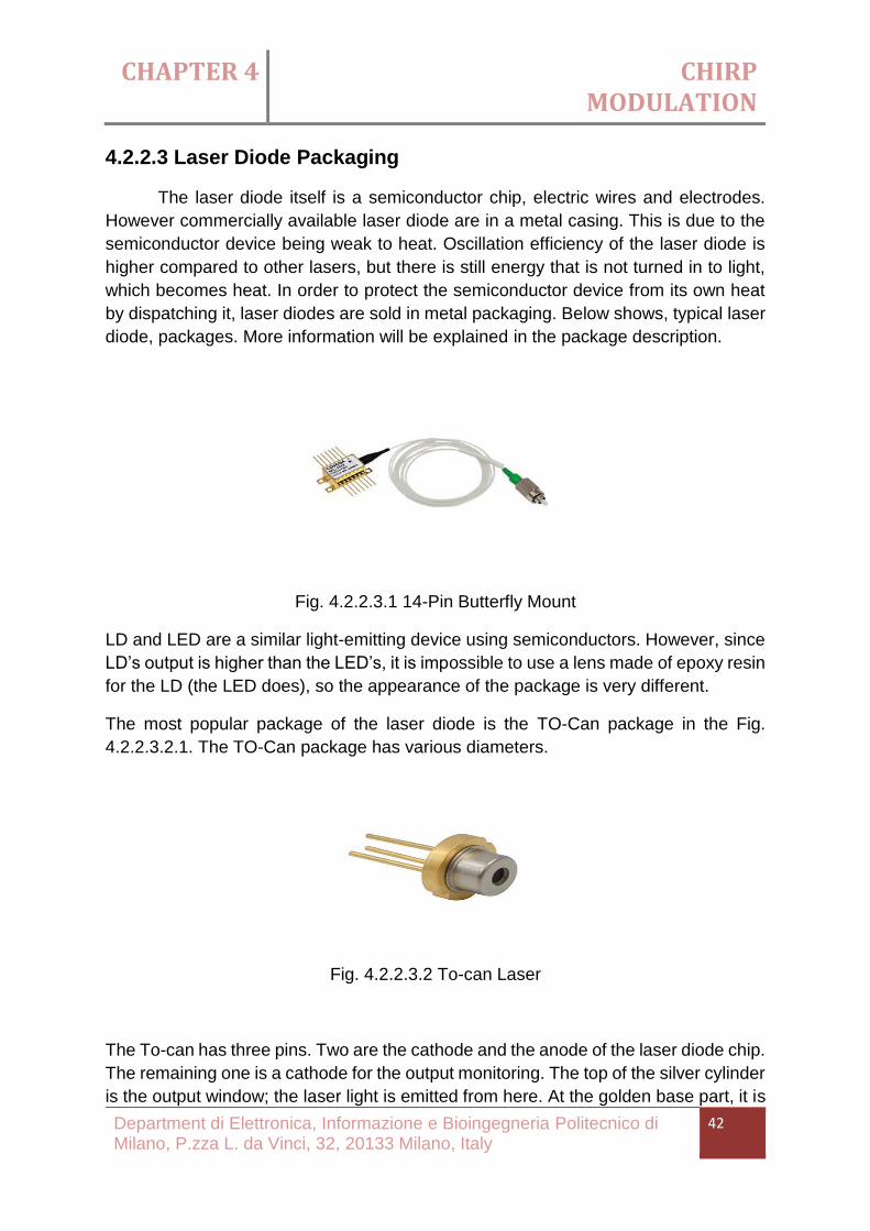
CHAPTER 4 CHIRP MODULATION
Department di Elettronica, Informazione e Bioingegneria Politecnico di Milano, P.zza L. da Vinci, 32, 20133 Milano, Italy
42
4.2.2.3 Laser Diode Packaging
The laser diode itself is a semiconductor chip, electric wires and electrodes.
However commercially available laser diode are in a metal casing. This is due to the
semiconductor device being weak to heat. Oscillation efficiency of the laser diode is
higher compared to other lasers, but there is still energy that is not turned in to light,
which becomes heat. In order to protect the semiconductor device from its own heat
by dispatching it, laser diodes are sold in metal packaging. Below shows, typical laser
diode, packages. More information will be explained in the package description.
Fig. 4.2.2.3.1 14-Pin Butterfly Mount
LD and LED are a similar light-emitting device using semiconductors. However, since
LD’s output is higher than the LED’s, it is impossible to use a lens made of epoxy resin
for the LD (the LED does), so the appearance of the package is very different.
The most popular package of the laser diode is the TO-Can package in the Fig.
4.2.2.3.2.1. The TO-Can package has various diameters.
Fig. 4.2.2.3.2 To-can Laser
The To-can has three pins. Two are the cathode and the anode of the laser diode chip.
The remaining one is a cathode for the output monitoring. The top of the silver cylinder
is the output window; the laser light is emitted from here. At the golden base part, it is

CHAPTER 4 CHIRP MODULATION
Department di Elettronica, Informazione e Bioingegneria Politecnico di Milano, P.zza L. da Vinci, 32, 20133 Milano, Italy
43
possible to attach the radiating plate. The following is a video that shows how the laser
is emitted from the laser diode of a TO-Can package.
Pin placement of a TO-Can package
Fig. 4.2.2.3.3 To-can pin alignment
There are various types pin placement points of a To-can package, as shown billow.
You’ll have to conform to the pin arrangement when you connect them.
Normal LDs of today used as an excitation light source are modulated and connected
to an optical fiber, as shown in the Fig. Most commonly used LD for fiber lasers and
optical amplifiers is 14-pin butterfly package.
A typical 14-pin butterfly package is a single emitter type, which consists of a LD chip,
optical isolator, Thermoelectric Cooler: TEC [1], and Photo Diode: PD for Laser beam
monitoring (Wavelength or output monitor), and is outputted by a optical fiber attached
to the ferrule.
Fig. 4.2.2.3.4 Description of package

CHAPTER 4 CHIRP MODULATION
Department di Elettronica, Informazione e Bioingegneria Politecnico di Milano, P.zza L. da Vinci, 32, 20133 Milano, Italy
44
Fig. 4.2.2.3.5 Structural blue print of fiber
Fig. 4.2.2.3.4/5 the (4) appearance (with FBG) and (5) package content of a 14-pin
butterfly package’s fiber pigtail.
The LD is sub-mounted to a Peltier device (TEC) for temperature control purpose. The
laser outputted from the LD is focused into the optical fiber (single-mode, multi-mode,
polarization-maintaining, large-diameter fiber etc.) by a micro lens. If there is a monitor
PD (here a PIN Diode: p-intrinsic-n Photo Diode [2]), output can be monitored. After
precise alignment they are fixed by YAG laser welding. Table shows the fiber pigtail
LD used as excitation LD for fiber lasers [6-9]. A single-mode fiber: SMF pigtail LD can
be fused with a SMF optic fiber, and mainly used for exciting rare-earth-doped SMF.
A multi-mode fiber: SMF pigtail LD can be fused with the excitation port of an excitation
combiner, and used mainly for exciting double-clad fiber DCF.

CHAPTER 5 SIMULATION AND EXPERIMENTAL RESULTS
Department di Elettronica, Informazione e Bioingegneria Politecnico di Milano, P.zza L. da Vinci, 32, 20133 Milano, Italy
45
5.1 Chirp impact on phase fringes measurement
5.1.1 Phase-Chirp Simulation
In Fig. 5.1.1.1 when ν is fixed, fiber length is directly proportional to the fringes. That
is why it will be linear.
In Fig. 5.1.1.2 when fiber length (L) is fixed, same reason.
In Fig. 5.1.1.3 when both ν & L is fixed, then also it has linear but when you increase
temperature, we observe some change in fringes.
Fig. 5.1.1.1 Simulation for fringes with fiber length
Fig. 5.1.1.2 Simulation for fringes depends on wavelength
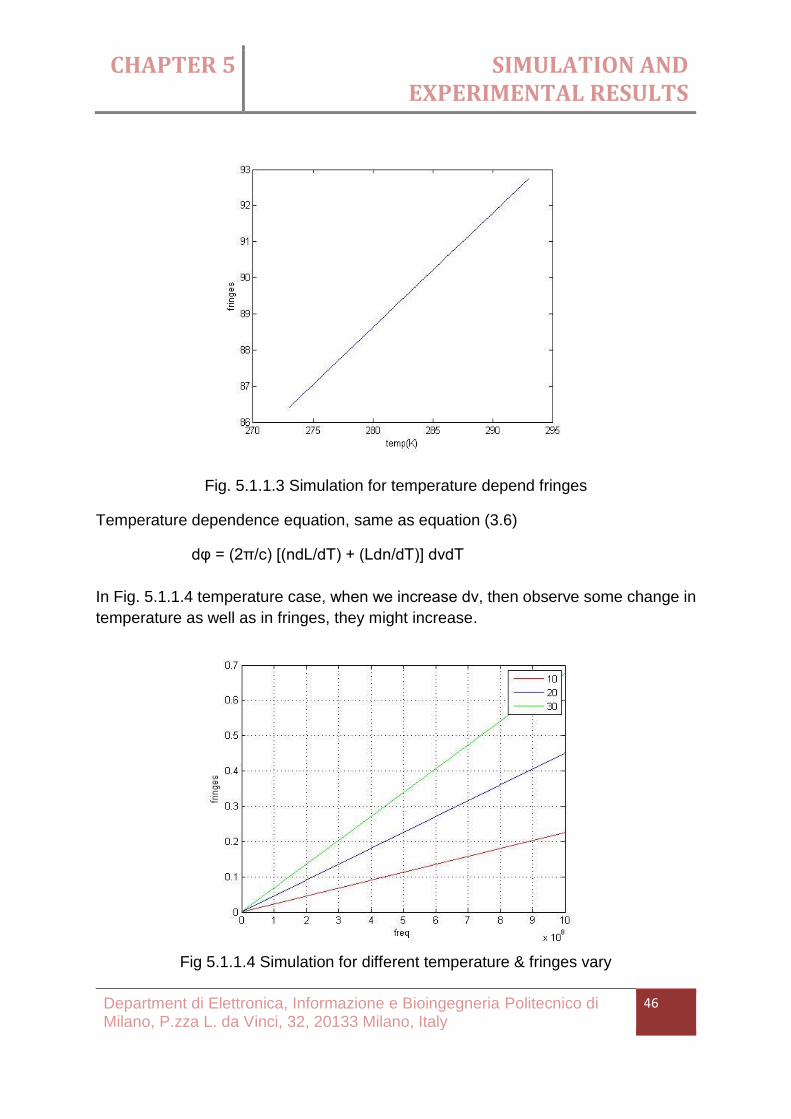
CHAPTER 5 SIMULATION AND EXPERIMENTAL RESULTS
Department di Elettronica, Informazione e Bioingegneria Politecnico di Milano, P.zza L. da Vinci, 32, 20133 Milano, Italy
46
Fig. 5.1.1.3 Simulation for temperature depend fringes
Temperature dependence equation, same as equation (3.6)
dφ = (2π/c) [(ndL/dT) + (Ldn/dT)] dνdT
In Fig. 5.1.1.4 temperature case, when we increase dν, then observe some change in
temperature as well as in fringes, they might increase.
Fig 5.1.1.4 Simulation for different temperature & fringes vary

CHAPTER 5 SIMULATION AND EXPERIMENTAL RESULTS
Department di Elettronica, Informazione e Bioingegneria Politecnico di Milano, P.zza L. da Vinci, 32, 20133 Milano, Italy
47
5.1.2 Chirp Measurement Setup
Fig. 5.1.2.1 Chirp setup
In Fig. 5.1.2.1 it shows how to observe the chirp. Starting laser modulator is provide
the variable current how much required for the laser. Wave shaper passed that so it
was distortion synthesis in which complex spectra are produced from simple tones by
altering the shape of the waveforms. So we can see the graph in oscilloscope & for
tracing I used wavelength observer.
Fig 5.1.2.2 Setup Configuration
Laser Laser
Modulator Wave Shaper
CRO
Wavelength
observer

CHAPTER 5 SIMULATION AND EXPERIMENTAL RESULTS
Department di Elettronica, Informazione e Bioingegneria Politecnico di Milano, P.zza L. da Vinci, 32, 20133 Milano, Italy
48
5.1.3 VCSEL Laser Chirp
• I use VCSEL laser to calculate the chirp.
• I modulate the frequency & amplitude-using simulator.
• Then using laser diode controller to control the current & with the help of
analyzer, we can see the difference in two waveform.
• Difference in chirp is 1.365nm.
Fig. 5.1.3 Vcsel result

CHAPTER 5 SIMULATION AND EXPERIMENTAL RESULTS
Department di Elettronica, Informazione e Bioingegneria Politecnico di Milano, P.zza L. da Vinci, 32, 20133 Milano, Italy
49
5.1.4 DFB/TO-CAN Laser Chirp
• Now use DSB laser to calculate the chirp.
• I have to fix the current then after I have to measure the laser wavelength.
Also using temperature controller.
• Balance the wave shaper using Matlab file.
• Then using waveform generator to give few MHz & with the help of
oscilloscope we can see the difference of two waveform.
• Difference in chirp is 0.5 nm.
Fig. 5.1.4.1 DFB result
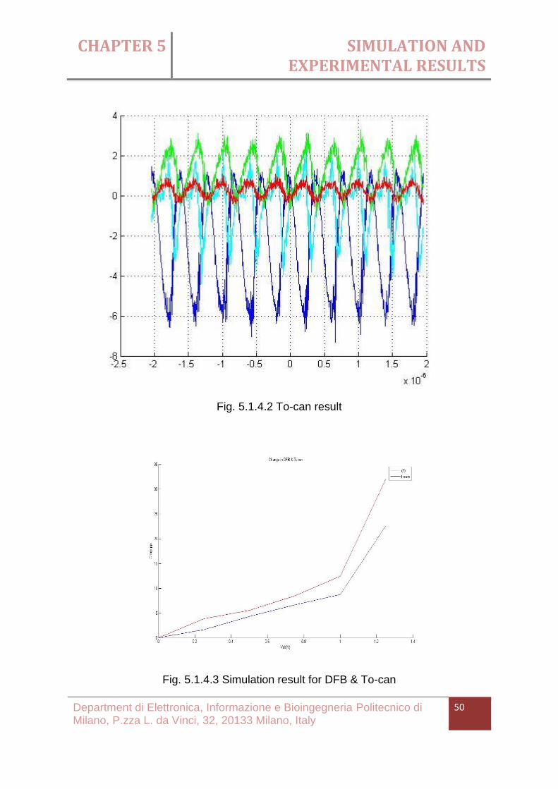
CHAPTER 5 SIMULATION AND EXPERIMENTAL RESULTS
Department di Elettronica, Informazione e Bioingegneria Politecnico di Milano, P.zza L. da Vinci, 32, 20133 Milano, Italy
50
Fig. 5.1.4.2 To-can result
Fig. 5.1.4.3 Simulation result for DFB & To-can

CHAPTER 5 SIMULATION AND EXPERIMENTAL RESULTS
Department di Elettronica, Informazione e Bioingegneria Politecnico di Milano, P.zza L. da Vinci, 32, 20133 Milano, Italy
51
5.2 Coherent fiber optic temperature sensor
5.2.1 Experimental setup with 3x3 coupler
Fig. 5.2.1.1 Coupler setup
In Fig 5.2.1.1 it shows how to perform fiber that was related to temperature using 3x3
coupler. Starting from pc that was given amplitude using Lab-view software then
function generator provide frequency to laser modulator as well as oscilloscope you
can see how much frequency given to laser modulator. Laser modulator provide the
variable current how much required for the laser. That was given by 1 of coupler end
and others 2 goes to photodiodes. Other side 2 ends are using fiber with mirror (one
is sensing arm & reference arm). In sensing arm I used 1 meter external fiber which is
dip in water so I observe some changes in fringes when temperature is increases.
Fringes will be increases but at the threshold level after fringes will be decreases if
you increase the temperature.
PC
Laser
Modulator
Laser
3X3
Coupler Photodiode1
Photodiode2
Fiber with
Mirror 1
Fiber with
Mirror 2
Boiler
Oscilloscope
Function Generator
Oscilloscope

CHAPTER 5 SIMULATION AND EXPERIMENTAL RESULTS
Department di Elettronica, Informazione e Bioingegneria Politecnico di Milano, P.zza L. da Vinci, 32, 20133 Milano, Italy
52
Fig 5.2.1.2 Setup for 3x3 coupler
In Fig 5.2.1.2 you can see the set up diagram which includes the instruments that can
performed 3x3 coupler. Moreover, I’ll attach a fig. 5.2.1.3 which includes fiber with
inside boiler and heater.
Fig 5.2.1.3 Fiber dip in water with heating

CHAPTER 5 SIMULATION AND EXPERIMENTAL RESULTS
Department di Elettronica, Informazione e Bioingegneria Politecnico di Milano, P.zza L. da Vinci, 32, 20133 Milano, Italy
53
5.2.2 Temperature experimental characterisations
In Fig 5.2.2.1 it shows 3 different colors which contain 20, 40 & 60 degree temperature
in real time oscilloscope. After every step, it will increase the fringes.
Fig. 5.2.2.1 Simulation for different temperature

CHAPTER 5 SIMULATION AND EXPERIMENTAL RESULTS
Department di Elettronica, Informazione e Bioingegneria Politecnico di Milano, P.zza L. da Vinci, 32, 20133 Milano, Italy
54
Fig.5.2.2.2 Mean & Std with different temperature
These curves refers to experimental results obtained with the same coherent setup
but with a different unbalanced length between the sensing and reference arm. It is
shown that Fig. 5.2.2.2, obtained with a longer unbalanced, guarantees a higher
sensitivity as, for the same temperature range variation, a higher number of fringes is
obtained with respect to the case of Fig. 5.2.2.3. Measurements confirm a linear
response of the coherent setup with respect to temperature variations with a good
standard deviation of around +/-10% with respect to the mean fringe number, thus
proving the feasibility of the proposed fiber optic technique for local temperature
measures.

CHAPTER 5 SIMULATION AND EXPERIMENTAL RESULTS
Department di Elettronica, Informazione e Bioingegneria Politecnico di Milano, P.zza L. da Vinci, 32, 20133 Milano, Italy
55
Fig. 5.2.2.3 Simulation for different temperature vary 20 – 75o

CHAPTER 6 CONCLUSIONS
Department di Elettronica, Informazione e Bioingegneria Politecnico di Milano, P.zza L. da Vinci, 32, 20133 Milano, Italy
56
In this work of thesis, a fiber optic sensor for local temperature measurement
has been presented. Fiber optic temperature sensors are already available on the
market, mainly based on FBG (Fiber-Bragg-Grating) or phosphors tips technology.
However, these solutions are still too expensive and not affordable for many industrial
applications. Fiber optic coherent technology represents instead a new and cost-
effective solution with multipurpose sensing capabilities. In the present work, this
approach has been exploited and specialized for temperature measurements.
After a brief introduction on the advantages offered by fiber optic sensors with respect
to electrical ones and on the different typologies of temperature fiber optic sensors
that have already been developed, the focus has been put on the main peculiarities of
this new coherent approach with respect to traditional interferometric setups. In
particular, it has been shown that the present approach solves two. main issues that
have till now prevented the actual in-field applicability of highly sensitive interferometric
schemes., that is, the need of an active-feedback stabilization of the interferometric
working point (quadrature point) and the occurrence of signal fading due to signal
polarization fluctuations. The former issue is solved by means of a passive coherent
receiver, which simultaneously provides the in-face and quadrature components of the
interferometric signal, allowing to always recovering the correct phase signal
information regardless of the interferometric working point. Polarization fading issue
instead has been solved by exploiting Faraday Rotation Mirrors (FRM) at the end of
the reference and sensing arms, which guarantees a complete compensation of all
polarization changes of the optical signal due to environmental perturbations acting on
the fiber. In particular, in the present work a 3x3 fiber optic coupler has been used as
a passive coherent receiver which, together with FRM, constitutes standard
components of optical communications, thus proving how the hardware core of this
coherent approach to sensing is a true cost-effective solution.
Moreover, the measurement of a quasi-static parameter, like temperature, has
required introducing a modulation inside the basic coherent scheme in order to obtain
a dynamic measurement of temperature, which allows better performance in term of
accuracy and sensitivity with respect to static measurements. Thus in the present work
it has been analyzed, both theoretically and through simulations, how to apply and
optimize the modulation of the optical source wavelength. This wavelength modulation
in coherent detection scheme transducers in the generation of phase fringes whose
number depends on the optical length of the sensing fiber arm.
If variation of the optical sensing length occurs, as for example due to an increase in
the local temperature, the number of phase fringes varies and allows detecting and
recovering the temperature variation information.

CHAPTER 6 CONCLUSIONS
Department di Elettronica, Informazione e Bioingegneria Politecnico di Milano, P.zza L. da Vinci, 32, 20133 Milano, Italy
57
In particular, the chirp of three different laser sources, a DFB laser, To-can laser and
a VCSEL has been characterized in order to evaluate the optical source capable to
guarantee the optimal compromise between high source coherence and large
wavelength modulation. Indeed these two parameters determine the final accuracy of
the proposed measurement technique. VCSEL ended up to be the optimal source and
thus has been exploited in the experimental setup that has been arranged to carry out
temperature measurements with the coherent fiber optic sensing approach.
Preliminary results proved the feasibility of the proposed techniques in reconstructing
temperature profiles with a temperature accuracy of few degrees in a range between
20- 70C°. Future works will follows to extend the measurement range and the sensor
measurement accuracy by selecting special protective fiber coatings and by exploiting
more optimized laser optical sources.
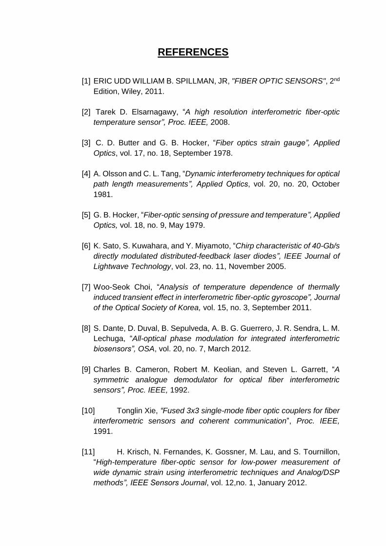
REFERENCES
[1] ERIC UDD WILLIAM B. SPILLMAN, JR, "FIBER OPTIC SENSORS", 2nd
Edition, Wiley, 2011.
[2] Tarek D. Elsarnagawy, “A high resolution interferometric fiber-optic
temperature sensor”, Proc. IEEE, 2008.
[3] C. D. Butter and G. B. Hocker, “Fiber optics strain gauge”, Applied
Optics, vol. 17, no. 18, September 1978.
[4] A. Olsson and C. L. Tang, “Dynamic interferometry techniques for optical
path length measurements”, Applied Optics, vol. 20, no. 20, October
1981.
[5] G. B. Hocker, “Fiber-optic sensing of pressure and temperature”, Applied
Optics, vol. 18, no. 9, May 1979.
[6] K. Sato, S. Kuwahara, and Y. Miyamoto, “Chirp characteristic of 40-Gb/s
directly modulated distributed-feedback laser diodes”, IEEE Journal of
Lightwave Technology, vol. 23, no. 11, November 2005.
[7] Woo-Seok Choi, “Analysis of temperature dependence of thermally
induced transient effect in interferometric fiber-optic gyroscope”, Journal
of the Optical Society of Korea, vol. 15, no. 3, September 2011.
[8] S. Dante, D. Duval, B. Sepulveda, A. B. G. Guerrero, J. R. Sendra, L. M.
Lechuga, “All-optical phase modulation for integrated interferometric
biosensors”, OSA, vol. 20, no. 7, March 2012.
[9] Charles B. Cameron, Robert M. Keolian, and Steven L. Garrett, “A
symmetric analogue demodulator for optical fiber interferometric
sensors”, Proc. IEEE, 1992.
[10] Tonglin Xie, “Fused 3x3 single-mode fiber optic couplers for fiber
interferometric sensors and coherent communication”, Proc. IEEE,
1991.
[11] H. Krisch, N. Fernandes, K. Gossner, M. Lau, and S. Tournillon,
“High-temperature fiber-optic sensor for low-power measurement of
wide dynamic strain using interferometric techniques and Analog/DSP
methods”, IEEE Sensors Journal, vol. 12,no. 1, January 2012.

[12] A. Ukil, Senior Member, IEEE, H. Braendle, and P. Krippner,
“Distributed Temperature Sensing: Review of Technology and
Applications,” IEEE Sensors Journal, vol. 12, no. 5, May 2012.
[13] B. W. Barr, S. H. Huttner, J. R. Taylor, B. Sorazu, M. V. Plissi, and
K. A. Strain, “Optical modulation techniques for length sensing and
control of optical cavities”, Applied Optics, vol. 46, no. 31, November
2007.
[14] D. Sigg, N. Mavalvala, J. Giaime, P. Fritschel, and D. Shoemaker,
"Signal extraction in a power-recycled Michelson interferometer with
Fabry–Perot arm cavities by use of a multiple-carrier frontal modulation
scheme", Applied Optics, vol. 37, no. 24, August 1998.
[15] Y. Lin, Y. Zou, and R. G. Lindquist, "A reflection-based localized
surface plasmon resonance fiber-optic probe for biochemical sensing",
OSA, vol. 2, no. 3, March 2011.
[16] E. Milcent, G. Olalde, J. F. Robert, D. Hernandez, and M.
Clement, "Influence of high temperatures on a fiber-optic probe for
temperature measurement", Applied Optics, vol. 33, no. 25, September
1994.
[17] Dong-Joon Lee, and John F. Whitaker, "An optical-fiber-scale
electro-optic probe for minimally invasive high-frequency field sensing",
OSA, vol. 16, no. 26, December 2008.
[18] L. Li, Li Xia, Z. Xie, and D. Liu, "All-fiber Mach-Zehnder
interferometers for sensing applications", OSA, vol. 20, no. 10, May
2012.
[19] Feifei Chen, Yi Jiang, and Lan Jiang, "3 × 3 coupler based
interferometric magnetic field sensor using a TbDyFe rod", Applied
Optics, vol. 54, no. 8, March 2015.
[20] Kwang Taek Kim and Kiu Ha Park, "Fiber-Optic Temperature
Sensor Based on Single Mode Fused Fiber Coupler", Journal of the
Optical Society of Korea, vol. 12, no. 3, September 2008.
[21] M. Gottlieb and G. B. Brandt, "Fiber-optic temperature sensor
based on internally generated thermal radiation", Applied Optics, vol. 20,
no. 19, October 1981.
[22] Stephanus J. Spammer, Pieter L. Swart, and Andre´ Booysen,
"Interferometric distributed optical-fiber sensor", Applied Optics, vol. 35,
no. 22, August 1996.
[23] Hairun Guo, Fufei Pang, Xianglong Zeng, Na Chen, Zhenyi Chen,
and Tingyun Wang, "Temperature sensor using an optical fiber coupler
with a thin film", Applied Optics, vol. 47, no. 19, July 2008.