arX

iv:c

s/07

0306

1v2

[cs

.IT

] 2

5 M

ar 2

008

Coding for Errors and Erasures in

Random Network Coding

Ralf Kotter∗

Institute for Communications EngineeringTU Munich

D-80333 Munichralf.koetter@tum.de

Frank R. Kschischang

The Edward S. Rogers Sr. Department

of Electrical and Computer EngineeringUniversity of Toronto

frank@comm.utoronto.ca

Submitted to IEEE Transactions on Information Theory

Submission Date: March 12, 2007. Revised: March 18, 2008.

Abstract

The problem of error-control in random linear network coding is considered. A“noncoherent” or “channel oblivious” model is assumed where neither transmitter norreceiver is assumed to have knowledge of the channel transfer characteristic. Motivatedby the property that linear network coding is vector-space preserving, informationtransmission is modelled as the injection into the network of a basis for a vector spaceV and the collection by the receiver of a basis for a vector space U . A metric on theprojective geometry associated with the packet space is introduced, and it is shown thata minimum distance decoder for this metric achieves correct decoding if the dimensionof the space V ∩U is sufficiently large. If the dimension of each codeword is restricted toa fixed integer, the code forms a subset of a finite-field Grassmannian, or, equivalently,a subset of the vertices of the corresponding Grassmann graph. Sphere-packing andsphere-covering bounds as well as a generalization of the Singleton bound are providedfor such codes. Finally, a Reed-Solomon-like code construction, related to Gabidulin’sconstruction of maximum rank-distance codes, is described and a Sudan-style “list-1”minimum distance decoding algorithm is provided.

∗Supported in part by DARPA ITMANET W911NF-07-I-0029.

1

1. Introduction

Random network coding [1–3] is a powerful tool for disseminating information in networks,yet it is susceptible to packet transmission errors caused by noise or intentional jamming.Indeed, in the most naive implementations, a single error in one received packet would typ-ically render the entire transmission useless when the erroneous packet is combined withother received packets to deduce the transmitted message. It might also happen that insuffi-ciently many packets from one generation reach the intended receivers, so that the problemof deducing the information cannot be completed.

In this paper we formulate a coding theory in the context of a “noncoherent” or “channeloblivious” transmission model for random linear network coding that captures the effectsboth of errors, i.e., erroneously received packets, and of erasures, i.e., insufficiently manyreceived packets. We are partly motivated by the close analogy between the Fq-linear channelproduced in random linear network coding and the C-linear channel produced in noncoherentmultiple-antenna channels [4], where neither the transmitter nor the receiver is assumed tohave knowledge of the channel transfer characteristic. In contrast with previous approachesto error control in random linear network coding, e.g., [5–8], the noncoherent transmissionstrategy taken in this paper is oblivious to the underlying network topology and to theparticular linear network coding operations performed at the various network nodes. Here,information is encoded in the choice at the transmitter of a vector space (not a vector), andthe choice of vector space is conveyed via transmission of a generating set for the space.

Just as codes defined on the complex Grassmann manifold play an important role in non-coherent multiple-antenna channels [4], we find that codes defined in an appropriate Grass-mannian associated with a vector space over a finite field play an important role here, butwith a different metric associated with the structure of the corresponding Grassman graph.

The standard, widely advocated approach to random linear network coding (see, e.g., [2])involves transmission of packet “headers” that are used to record the particular linear com-bination of the components of the message present in each received packet. As we willshow, this “uncoded” transmission may be viewed as a particular code of subspaces, but a“suboptimal” one, in the sense that the Grassmannian contains more spaces of a particulardimension than those obtained by prepending a header to the transmitted packets. Indeed,the very notion of a header or local and global encoding vectors, crucial in [2, 3, 8], is mootin our context.

A somewhat more closely related approach is that of [9], which deals with reliable commu-nication in networks with so-called “Byzantine adversaries,” who are are assumed to havesome ability to inject packets into the network and sometimes also to eavesdrop (i.e., readpackets transmitted in the network) [10]. It is shown that an optimal communication rate(which depends on the adversary’s eavesdropping capability) is achievable with high prob-ability with codes of sufficiently long block length. The work of this paper, in contrast,concentrates more on the possibility of code constructions with a prescribed deterministiccorrection capability, which, however, asymptotically can achieve the same rates as would

2

be achieved in the so-called “omniscient adversary model” of [9].

The remainder of this paper is organized as follows.

In Section 2, we introduce the “operator channel” as a concise and convenient abstractionof the channel encountered in random linear network coding, when neither transmitter norreceiver has knowledge of the channel transfer characteristics. The input and output alphabetfor an operator channel is the projective geometry (the set of all subspaces) associated witha given vector space over a finite field Fq. In Section 3, we define a metric on this set that isnatural and suitable in the context of random linear network coding. The transmitter selectsa space V for transmission, indicating this choice by injection into the network of a set ofpackets that generate V . The receiver collects packets that span some received space U . Weshow that correct decoding is possible with a minimum distance decoder if the dimension ofthe space V ∩ U is sufficiently large, just as correct decoding in the conventional Hammingmetric is possible if the received vector u agrees with the transmitted vector v in sufficientlymany coordinates.

We will usually confine our attention to constant-dimension codes, i.e., codes in which allcodewords have the same dimension. In this case, the code is a subset of the correspondingGrassmannian, or, equivalently, a subset of the vertices of the corresponding Grassmanngraph. Coding in the Grassmann graph has been an active area of research in combinatorics[11–15], where the problem has been studied as a packing problem that arises naturally. InSection 4, we derive elementary coding bounds, analogous to the sphere-packing (Hamming)upper bounds and the sphere-covering (Gilbert-Varshamov) lower bounds for such codes. Bydefining an appropriate notion of puncturing, we also derive a Singleton bound. Asymptoticversions of these bounds are also given. Some Johnson-type bounds on constant dimensioncodes can be found in [16].

A notable application for constant-dimension codes is their use as so-called linear authenti-cation codes introduced by Wang, Xing and Safavi-Naini [17]. There, the properties of codesin the Grassmann graphs are used to detect tampering with an authenticated message. Theauthors of [17] describe a construction by which constant-dimension codes that are suitablefor linear authentication can be obtained from rank-distance codes, in particular from themaximum rank-distance codes of Gabidulin [18]. In Section 5 we revisit this construction inthe context of the coding metric defined in this paper, and we show that these codes achievethe Singleton bound asymptotically. The main result of Section 5 is the development ofan efficient Sudan-style “list-1” minimum distance decoding algorithm for these codes. Arelated polynomial-reconstruction-based decoder for Gabidulin codes has been described byLoidreau [19]. The connection between rank-metric codes and a generalized rank-metricdecoding problem induced by random linear network coding is explored in [20].

3

2. Operator Channels

We begin by formulating our problem for the case of a single unicast, i.e., communicationbetween a single transmitter and a single receiver. Generalization to multicasting is straight-forward.

To capture the essence of random linear network coding, recall [2, 3] that communicationbetween transmitter and receiver occurs in a series of rounds or “generations;” during eachgeneration, the transmitter injects a number of fixed-length packets into the network, eachof which may be regarded as a row vector of length N over a finite field Fq. These packetspropagate through the network, possibly passing through a number of intermediate nodesbetween transmitter and receiver. Whenever an intermediate node has an opportunity tosend a packet, it creates a random Fq-linear combination of the packets it has available andtransmits this random combination. Finally, the receiver collects such randomly generatedpackets and tries to infer the set of packets injected into the network. There is no assumptionhere that the network operates synchronously or without delay or that the network is acyclic.

The set of successful packet transmissions in a generation induces a directed multigraph withthe same vertex set as the network, in which edges denote successful packet transmissions.The rate of information transmission (packets per generation) between the transmitter andthe receiver is upper-bounded by the min-cut between these nodes, i.e., by the minimumnumber of edge deletions in the graph that would cause the separation of the transmitterand the receiver. It is known that random linear network coding in Fq is able to achieve atransmission rate that achieves the min-cut rate with probability approaching one as q → ∞[3].

Let {p1, p2, . . . , pM}, pi ∈ FNq denote the set of injected vectors. In the error-free case, the

receiver collects packets yj, j = 1, 2, . . . , L where each yj is formed as yj =∑M

i=1 hj,ipi withunknown, randomly chosen coefficients hj,i ∈ Fq.

We note that a priori L is not fixed and the receiver would normally collect as many packetsas possible. However, as noted above, properties of the network such as the min-cut betweenthe transmitter and the receiver may influence the joint distribution of the hi,j and, at somepoint, there will be no benefit from collecting further redundant information.

If we choose to consider the injection of T erroneous packets, this model is enlarged to includeerror packets et, t = 1, . . . , T to give

yj =

M∑

i=1

hj,ipi +

T∑

t=1

gj,tet,

where again gj,t ∈ Fq are unknown random coefficients. Note that since these erroneouspackets may be injected anywhere within the network, they may cause widespread errorpropagation. In particular, if gj,1 6= 0 for all j, even a single error packet e1 has the potentialto corrupt each and every received packet.

4

In matrix form, the transmission model may be written as

y = Hp + Ge, (1)

where H and G are random L×M and L×T matrices, respectively, p is the M ×N matrixwhose rows are the transmitted vectors, y is the L × N matrix whose rows are the receivedvectors, and e is the T × N matrix whose rows are the error vectors.

The network topology will certainly impose some structure on the matrices H and G. Forexample, H may be rank-deficient if the min-cut between transmitter and receiver is notlarge enough to support the transmission of M independent packets during the lifetime ofone generation1. While the possibility may exist to exploit the structure of the network,in the strategy adopted in this paper we do not take any possibly finer structure of thematrix H into account. Indeed, any such fine structure can be effectively obliterated byrandomization at the source, i.e., if, rather than injecting packets pi into the network, thetransmitter were instead to inject random linear combinations of the pi.

At this point, since H is random, we may ask what property of the injected sequence ofpackets remains invariant in the channel described by (1), even in the absence of noise(e = 0)? Since H is a random matrix, all that is fixed by the product Hp is the row spaceof p. Indeed, as far as the receiver is concerned, any of the possible generating sets for thisspace are equivalent. We are led, therefore, to consider information transmission not via thechoice of p, but rather by the choice of the vector space spanned by the rows of p. This simpleobservation is at the heart of the channel models and transmission strategies considered inthis paper. Indeed, with regard to the vector space selected by the transmitter, the onlydeleterious effect that a multiplication with H may have is that Hp may have smaller rankthan p, due to, e.g., an insufficient min-cut or packet erasures, in which case Hp generatesa subspace of the row space of p.

Let W be a fixed N -dimensional vector space over Fq. All transmitted and received packetswill be vectors of W ; however, we will describe a transmission model in terms of subspaces ofW spanned by these packets. Let P(W ) denote the set of all subspaces of W , an object oftencalled the projective geometry of W . The dimension of an element V ∈ P(W ) is denotedas dim(V ). The sum of two subspaces U and V of W is U + V = {u + v : u ∈ U, v ∈ V }.Equivalently, U +V is the smallest subspace of W containing both U and V . If U ∩V = {0},i.e., if U and V have trivial intersection, then the sum U + V is a direct sum, denoted asU ⊕ V . Clearly dim(U ⊕ V ) = dim(U) + dim(V ). For any subspaces U and V we haveV = (U ∩V )⊕V ′ for some subspace V ′ isomorphic to the quotient space V/(U ∩V ). In thiscase, U + V = U + ((U ∩ V ) ⊕ V ′) = U ⊕ V ′.

For integer k > 0, we define a stochastic operator Hk, called an “erasure operator,” thatoperates on the subspaces of W . If dim(V ) > k, then Hk(V ) returns a randomly chosenk-dimensional subspace of V ; otherwise, Hk(V ) returns V . For the purposes of this paper,

1This statement can be made precise once the precise protocol for transmission of a generation has beenfixed. However, for the purpose of this paper it is sufficient to summarily model “rank deficiency” as onepotential cause of errors.

5

the distribution of Hk(V ) is unimportant; for example, it could be chosen to be uniform.Given two subspaces U and V of W , it is always possible to realize U as U = Hk(V )⊕E forsome subspace E of W , assuming that that k = dim(U ∩ V ) and that Hk(U) realizes U ∩V .

We define the following “operator channel” as a concise transmission model for networkcoding.

Definition 1 An operator channel C associated with the ambient space W is a channel with

input and output alphabet P(W ). As described above, the channel input V and channel

output U can always be related as

U = Hk(V ) ⊕ E, (2)

where k = dim(U ∩ V ) and E is an error space. In transforming V to U , we say that the

operator channel commits ρ = dim(V ) − k erasures and t = dim(E) errors.

Note that we have chosen to model the error space E as intersecting trivially with thetransmitted subspace V , and thus the choice of E is not independent of V . However, ifwe were to model the received space as U = Hk(V ) + E for an arbitrary error space E,then, since E always decomposes for some space E ′ as E = (E ∩ V ) ⊕ E ′, we would getU = Hk(V ) + (E ∩ V ) ⊕ E ′ = Hk′(V ) ⊕ E ′ for some k′ > k. In other words, components ofan error space E that intersect with the transmitted space V would only be helpful, possiblydecreasing the number of erasures seen by the receiver.

In summary, an operator channel takes in a vector space and puts out another vector space,possibly with erasures (deletion of vectors from the transmitted space) or errors (additionof vectors to the transmitted space).

This definition of an operator channel makes a very clear connection between network cod-ing and classical information theory. Indeed, an operator channel can be seen as a standarddiscrete memoryless channel with input and output alphabet P(W ). By imposing a channellaw, i.e., transition probabilities between spaces, it would (at least conceptually) be straight-forward to compute capacity, error exponents, etc. Indeed, only slight extensions would benecessary concerning the ergodic behavior of the channel. For the present paper we constrainour attention to the question of constructing good codes in P(W ), which is an essentiallycombinatorial problem. The codes we construct may be regarded as “one-shot” codes, i.e.,codes of length one, since the transmission of a codeword will induce exactly one use of theoperator channel.

3. Coding for Operator Channels

Definition 1 concisely captures the effect of random linear network coding in the presenceof networks with erasures, varying min-cuts and/or erroneous packets. Indeed, we will show

6

how to construct codes for this channel that correct combinations of errors and erasures.Before we give such a construction we need to define a suitable metric.

3.1. A Metric on P(W )

Let Z+ denote the set of non-negative integers. We define a function d : P(W )×P(W ) → Z+

byd(A, B) := dim(A + B) − dim(A ∩ B). (3)

Since dim(A + B) = dim(A) + dim(B) − dim(A ∩ B), we may also write

d(A, B) = dim(A) + dim(B) − 2 dim(A ∩ B)

= 2 dim(A + B) − dim(A) − dim(B).

The following lemma is a cornerstone for code design for the operator channel of Definition 1.

Lemma 1 The function

d(A, B) := dim(A + B) − dim(A ∩ B)

is a metric for the space P(W ).

Proof. We need to check that for all subspaces A, B, X ∈ P(W ) we have: i) d(A, B) > 0with equality if and only if A = B, ii) d(A, B) = d(B, A), and iii) d(A, B) 6 d(A, X) +d(X, B). The first two conditions are clearly true and so we focus on the third condition,the triangle inequality. We have

1

2(d(A, B) − d(A, X) − d(X, B)) = dim(A ∩ X) + dim(B ∩ X) − dim(X) − dim(A ∩ B)

= dim(A ∩ X + B ∩ X) − dim(X)︸ ︷︷ ︸

60

+ dim(A ∩ B ∩ X) − dim(A ∩ B)︸ ︷︷ ︸

60

6 0,

where the first inequality follows from the property that A∩X +B∩X ⊆ X and the secondinequality follows from the property that A ∩ B ∩ X ⊆ A ∩ B.

Remark: The fact that d(A, B) is a metric also follows from the fact that this quantity repre-sents the distance of a geodesic between A and B in the undirected Hasse graph representingthe lattice of subspaces of W [11] partially ordered by inclusion, i.e., where X � Y if andonly if X is a subspace of Y . In this graph, the vertices correspond to the elements of P(W )and an edge joins a subspace X with a subspace Y if and only if | dim(X)−dim(Y )| = 1 and

7

either X ⊂ Y or Y ⊂ X. Just as the hypercube provides the appropriate setting for codingin the Hamming metric, the undirected Hasse graph represents the appropriate setting forcoding in the context considered here.

If a basis for W is fixed, then since W is an N -dimensional vector space over Fq, the elementsof W may be represented by N -tuples of Fq-valued coordinates with respect to this basis.We take the usual inner product between vectors u = (u1, . . . , uN) and v = (v1, . . . , vN) as(u, v) =

∑Ni=1 uivi. If U is a k-dimensional subspace of W , then the orthogonal subspace

U⊥ = {v ∈ W : (u, v) = 0 for all u ∈ U}

is a space of dimension N − k. It is well known that for any subspaces U and V of W that(U⊥)⊥ = U ,

(U + V )⊥ = U⊥ ∩ V ⊥, and (U ∩ V )⊥ = U⊥ + V ⊥.

It follows that

d(U⊥, V ⊥) = dim(U⊥ + V ⊥) − dim(U⊥ ∩ V ⊥)

= dim((U ∩ V )⊥) − dim((U + V )⊥)

= (N − dim(U ∩ V )) − (N − dim(U + V ))

= dim(U + V ) − dim(U ∩ V )

= d(U, V ). (4)

Thus the distance between subspaces U and V is perfectly mirrored by the distance betweenthe orthogonal subspaces U⊥ and V ⊥.

3.2. Codes

Let W be an N -dimensional vector space over Fq. A code for an operator channel withambient space W is simply a nonempty subset of P(W ), i.e., a nonempty collection ofsubspaces of W .

The size of a code C is denoted by |C|. The minimum distance of C is denoted by

D(C) := minX,Y ∈C:X 6=Y

d(X, Y ).

The maximum dimension of the codewords of C is denoted by

ℓ(C) := maxX∈C

dim(X).

If the dimension of each codeword of C is the same, then C is said to be a constant-dimension

code.

In analogy with the (n, k, d) triple that describes the parameters of a classical linear errorcorrecting code of length n, dimension k and minimum Hamming distance d, a code C for

8

an operator channel with an N -dimensional ambient space over Fq is said to be of type[N, ℓ(C), logq |C|, D(C)].

The complementary code corresponding to a code C is the code C⊥ = {U⊥ : U ∈ C} obtainedfrom the orthogonal subspaces of the codewords of C. In view of (4), we have D(C⊥) = D(C).If C is a constant-dimension code of type [N, ℓ, M, D], then C⊥ is a constant-dimension codeof type [N, N − ℓ, M, D].

Before we study bounds and constructions of codes in P(W ), we need a proper definition ofrate. Let C ⊂ P(W ) be a code of type [N, ℓ, logq |C|, D]. To transmit a space V ∈ C wouldrequire the transmitter to inject up to ℓ(C) (basis) vectors from V into the network, corre-sponding to the transmission of Nℓ q-ary symbols. This motivates the following definition.

Definition 2 Let C be a code of type [N, ℓ, logq(|C|), D]. The normalized weight λ, the rate

R, and the normalized minimum distance δ of C are defined as

λ =ℓ

N, R =

logq(|C|)

Nℓand δ =

D

2ℓ.

The parameters λ, R and δ are quite natural. The normalized weight λ takes the role ofthe energy of a spherical code in Euclidean space, or the equivalent weight parameter forconstant weight codes. As such λ is naturally limited to the range [0, 1]. For constant-dimension codes, just as in the case of constant-weight codes, the interesting range canactually be limited to [0, 1

2] as any code C with ℓ > N/2 corresponds to the complementary

code C⊥ with ℓ < N/2 and having the identical distance properties. The definition of δ givesa natural range of [0, 1]. Indeed, a normalized distance of 1 could only be obtained by spaceshaving trivial intersection. The rate R of a code is restricted to the range [0, 1], with a rateof 1 only being approachable for λ → 0.

The fundamental code construction problem for the operator channel of Definition 1 thusbecomes the determination of achievable tuples [λ, R, δ] as the dimension of ambient space Nbecomes arbitrarily large. We note that this setup may lack physical reality since it assumesthat the network can operate with arbitrarily long packets; thus we will try to express ourresults for finite length N whenever possible. Furthermore, as noted above, the codes weconsider here are “one-shot” codes that induce just a single use of the operator channel. Insituations where the channel characteristics (such as the network min-cut) are time-varying,it may be interesting and useful to define codes that induce n uses of the operator channel,considering what performance is attainable as n → ∞. We will not pursue this direction inthis paper.

3.3. Error and Erasure Correction

A minimum distance decoder for a code C is one that takes the output U of an operatorchannel and returns a nearest codeword V ∈ C, i.e., a codeword V ∈ C satisfying, for allV ′ ∈ C, d(U, V ) 6 d(U, V ′).

9

The importance of the minimum distance D(C) for a code C ⊂ P(W ) is given in the followingtheorem, which provides the combined error-and-erasure-correction capability of C underminimum distance decoding. Define (x)+ as (x)+ := max{0, x}.

Theorem 2 Assume we use a code C for transmission over an operator channel. Let V ∈ Cbe transmitted, and let

U = Hk(V ) ⊕ E

be received, where dim(E) = t. Let ρ = (ℓ(C)−k)+ denote the maximum number of erasures

induced by the channel. If

2(t + ρ) < D(C), (5)

then a minimum distance decoder for C will produce the transmitted space V from the

received space U .

Proof. Let V ′ = Hk(V ). From the triangle inequality we have d(V, U) 6 d(V, V ′) +d(V ′, U) 6 ρ + t. If T 6= V is any other codeword in C, then D(C) 6 d(V, T ) 6 d(V, U) +d(U, T ), from which it follows that d(U, T ) > D(C) − d(V, U) > D(C) − (ρ + t). Providedthat the inequality (5) holds, then d(U, T ) > d(U, V ) and hence a minimum distance decodermust produce V .

Not surprisingly, given the symmetry in this setup between erasures (deletion of dimensionsdue to, e.g., an insufficient min-cut in the network or an unfortunate choice of coefficientsin the random linear network code) and errors (insertion of dimensions due to errors ordeliberate malfeasance), erasures and errors are equally costly to the decoder. This standsin apparent contrast with traditional error correction (where erasures cost less than errors);however, this difference is merely an accident of terminology. A perhaps more closely relatedclassical concept would be that of “insertions” and “deletions”.

If we can be sure that the projection operation is moot (expressed by choosing operatorHdim(W ) which operates as an identity on each subspace of W ) or that the network producesno errors (expressed by choosing the error space E = {0}), we get the following corollary.

Corollary 3 Assume we use a code C for transmission over an operator channel where V ∈ Cis transmitted. If

U = Hdim(W )(V ) ⊕ E = V ⊕ E

is received, and if 2t < D(C) where dim(E) = t, then a minimum distance decoder for C will

produce V . Symmetrically, if

U = Hk(V ) ⊕ {0} = Hk(V )

is received, and if 2ρ < D(C) where ρ = (ℓ(C) − k)+, then a minimum distance decoder for

C will produce V .

In other words, the first part of the corollary states that in the absence of erasures a minimumdistance decoder uniquely corrects errors up to dimension

t 6 ⌊D(C) − 1)

2⌋,

10

precisely in parallel to the standard error-correction situation.

3.4. Constant-Dimension Codes

In the context of network coding, it is natural to consider codes in which each codewordhas the same dimension, as knowledge of the codeword dimension can be exploited by thedecoder to initiate decoding. Constant-dimension codes are analogous to constant-weightcodes in Hamming space (in which every codeword has constant Hamming weight) or tospherical codes in Euclidean space (in which every codeword has constant energy).

As noted above, when considering constant-dimension codes we may restrict ourselves tocodes of type [N, ℓ, M, D] with ℓ 6 N − ℓ, since a code of type [N, ℓ, M, D] with ℓ > N − ℓmay be replaced with its complementary code C⊥ while maintaining all distance properties(therefore maintaining all error- and erasure-correcting capability).

Constant-dimension codes are naturally described as particular vertices of a so-called Grass-

mann graph, also called a q-Johnson scheme, where the latter name emphasizes that theseobjects constitute association schemes. A formal definition is given as follows.

Definition 3 Denote by P(W, ℓ) the set of all subspaces of W of dimension ℓ. This object

is known as a Grassmannian. The Grassmann graph GW,ℓ has vertex set P(W, ℓ) with an

edge joining vertices U and V if and only if d(U, V ) = 2.

Remark: It is well known that GW,ℓ is distance regular [21] and an association scheme withrelations given by the distance between spaces. As such, practically all techniques for boundsin the Hamming association scheme apply. In particular, sphere-packing and sphere-coveringconcepts have a natural equivalent formulation. We explore these directions in Section 4.We also note that the distance between two spaces U, V in P(W, ℓ) introduced in (3) is, likein the case of constant-weight codes in the Hamming metric, an even number equal to twicethe graph distance in the Grassmann graph.2 As noted Section 1, codes in the Grassmanngraph have been considered previously in [11–15,17].

When modelling the operation of random linear network coding by the operator channel ofDefinition 1, there is no further need to specify the precise network protocol. In particular,we assume the receiver knows that a codeword V from P(W, ℓ) was transmitted. In thissituation, a receiver could choose to collect packets until the collected packets, interpreted asvectors, span an ℓ-dimensional space. This situation would correspond to an operator channelof type U = Hℓ−t(E)(V ) ⊕ E, corresponding to t(E) erasures and t(E) errors. According to

Theorem 2 we can thus correct up to an error dimension ⌊D(C)−14

⌋. To some extent thisadditional factor of two reflects the choice of the distance measure as being twice the graphdistance in GW,ℓ. Note that this situation also would arise if the errors originated in network-coded transmissions through the min-cut edges in the graph. If the errors do not affect the

2Defining a distance as half of d(U, V ) would give non-integer values for packings in P(W ).

11

min cut but may have arisen anywhere else in the network, a receiver can choose to collectpackets until an ℓ + t(E) dimensional space V ⊕ E has been recovered.3 In this case the

error correction capability would increase to an error dimension ⌊D(C)−12

⌋. We do not studythe implications of this observation further in this paper, since the coding-theoretic goal ofconstructing good codes in P(W ) is not affected by this. Nevertheless, we point out that aproperly designed protocol can (and should) take advantage of these differences.

3.5. Examples of Codes

We conclude this section with two examples of codes in P(W, ℓ) .

Example 1 Let W be the vector space of N -tuples over Fq. Consider the set C ⊂ P(W, ℓ)of spaces Ui, i = 1, 2, . . . , |C| with generator matrices G(Ui) = (I|Ai) where I is an ℓ × ℓidentity matrix and the Ai are all possible ℓ × (N − ℓ) matrices over Fq. It is easy to seethat all G(Ui) generate different spaces, intersecting in subspaces of dimension at most ℓ− 1and that, hence, the minimum distance of the code is 2ℓ − 2(ℓ − 1) = 2. The code is aconstant-dimension code of type [N, ℓ, ℓ(N − ℓ), 2] with normalized weight λ = ℓ/N , rateR = 1 − λ and normalized distance δ = 1

λN.

The first example corresponds to a trivial code that offers no error protection at all. Whilethis code has been advocated widely for random linear network coding it is by no means theoptimal code for a given distance D = 2, as can be seen in the following example.

Example 2 Again let W be the space of vectors of length N . We now choose the codeC′ = P(W, ℓ), which yields a constant-dimension code of type [N, ℓ, logq |P(W, ℓ)|, 2] whichis clearly larger than the code C of Example 1. As explained in Section 4, |P(W, ℓ)| is equalto the Gaussian coefficient

[Nℓ

]

q.

We note that C′′, defined as C′′ =⋃ℓ

i=1 P(W, i) (no longer a constant-dimension code) isobviously an even bigger code (albeit with minimum distance D = 1) that can be usedfor random linear network coding while not using more network resources than C and C′.However, in contrast to C′, the receiver must be able to determine when the transmission ofthe code space is complete. This information is implicit in C′ and C since the dimension ofthe transmitted space is fixed beforehand.

In the next section we provide a few standard bounds for codes in our setup.

3Not knowing the effective dimension of E, i.e., the dimension of E/(E ∩ V ), in practice the receiverwould just collect as many packets as possible and attempt to reconstruct the corresponding space.

12

4. Bounds on Codes

4.1. Preliminaries

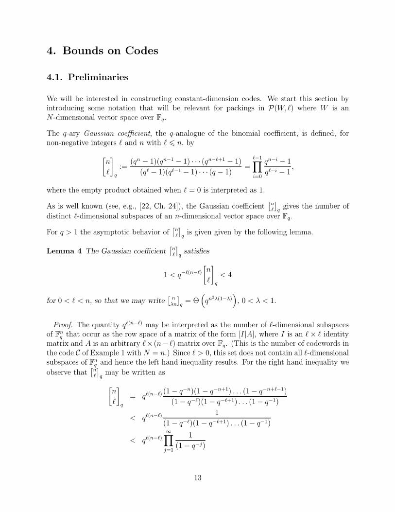
We will be interested in constructing constant-dimension codes. We start this section byintroducing some notation that will be relevant for packings in P(W, ℓ) where W is anN -dimensional vector space over Fq.

The q-ary Gaussian coefficient, the q-analogue of the binomial coefficient, is defined, fornon-negative integers ℓ and n with ℓ 6 n, by

[n

ℓ

]

q

:=(qn − 1)(qn−1 − 1) · · · (qn−ℓ+1 − 1)

(qℓ − 1)(qℓ−1 − 1) · · · (q − 1)=

ℓ−1∏

i=0

qn−i − 1

qℓ−i − 1,

where the empty product obtained when ℓ = 0 is interpreted as 1.

As is well known (see, e.g., [22, Ch. 24]), the Gaussian coefficient[nℓ

]

qgives the number of

distinct ℓ-dimensional subspaces of an n-dimensional vector space over Fq.

For q > 1 the asymptotic behavior of[nℓ

]

qis given given by the following lemma.

Lemma 4 The Gaussian coefficient[nℓ

]

qsatisfies

1 < q−ℓ(n−ℓ)

[n

ℓ

]

q

< 4

for 0 < ℓ < n, so that we may write[

nλn

]

q= Θ

(

qn2λ(1−λ))

, 0 < λ < 1.

Proof. The quantity qℓ(n−ℓ) may be interpreted as the number of ℓ-dimensional subspacesof Fn

q that occur as the row space of a matrix of the form [I|A], where I is an ℓ × ℓ identitymatrix and A is an arbitrary ℓ× (n− ℓ) matrix over Fq. (This is the number of codewords inthe code C of Example 1 with N = n.) Since ℓ > 0, this set does not contain all ℓ-dimensionalsubspaces of Fn

q and hence the left hand inequality results. For the right hand inequality we

observe that[nℓ

]

qmay be written as

[n

ℓ

]

q

= qℓ(n−ℓ) (1 − q−n)(1 − q−n+1) . . . (1 − q−n+ℓ−1)

(1 − q−ℓ)(1 − q−ℓ+1) . . . (1 − q−1)

< qℓ(n−ℓ) 1

(1 − q−ℓ)(1 − q−ℓ+1) . . . (1 − q−1)

< qℓ(n−ℓ)∞∏

j=1

1

(1 − q−j)

13

The function f(x) =∏∞

j=11

(1−xj)is the generating function of integer partitions [22, Ch. 15]

which is increasing in x. As we are interested in f(1/q) for q > 2, we find that

∞∏

j=1

1

1 − q−j6

∞∏

j=1

1

1 − 2−j= 1/Q0 < 4,

where Q0 ≈ 0.288788095 is a probabilistic combinatorial constant (see, e.g., [23]) that givesthe probability that a large, randomly chosen square binary matrix over F2 is nonsingular.

We remarked earlier that the Grassmann graph constitutes an association scheme, whichlets us use simple geometric arguments to give the standard sphere-packing upper boundsand sphere-covering lower bounds. In order to establish the bounds we need the notion of asphere.

Definition 4 Let W be an N dimensional vector space and let P(W, ℓ) be the set of ℓdimensional subspaces of W . The sphere S(V, ℓ, t) of radius t centered at a space V in

P(W, ℓ) is defined as the set of all subspaces U that satisfy d(U, V ) 6 2t,

S(V, ℓ, t) = {U ∈ P(W, ℓ) : d(U, V ) 6 2t}.

Note that we prefer to define the radius in terms of the graph distance in the Grassmanngraph. The radius can therefore take on any non-negative integer value.

Theorem 5 The number of spaces in S(V, ℓ, t) is independent of V and equals

|S(V, ℓ, t)| =t∑

i=0

qi2[ℓ

i

][N − ℓ

i

]

for t 6 ℓ.

Proof. The claim that S(V, ℓ, t) is independent of V follows from the fact that P(W, ℓ)constitutes a distance regular graph [21]. We give an expression for the number of spacesU that intersect V in an ℓ − i dimensional subspace. We can choose the ℓ − i dimensionalsubspace of intersection in

[ℓ

ℓ−i

]=[ℓi

]ways. Once this is done we can complete the subspace

in(qN − qℓ)(qN − qℓ+1) . . . (qN − qℓ+i−1)

(qℓ − qℓ−i)(qℓ − qℓ−i+1) . . . (qℓ − qℓ−1)= qi2

[N − ℓ

i

]

ways. Thus the cardinality of a shell of spaces at distance 2i around V equals qi2[N−ℓ

i

][ℓi

].

Summing the cardinality of the shells gives the theorem.

Note that |S(V, ℓ, t)| = |S(V, N − ℓ, t)|, as expected from (4).

14

4.2. Sphere-Packing and Sphere-Covering Bounds

We now can simply state the sphere-packing and sphere-covering bounds as follows:

Theorem 6 Let C be a collection of spaces in P(W, ℓ) such that D(C) > 2t, and let s =⌊ t−1

2⌋. The size of C must satisfy

|C| 6|P(W, ℓ)|

|S(V, ℓ, s)|=

[Nℓ

]

|S(V, ℓ, s)|<

[Nℓ

]

qs2[ℓs

][N−ℓ

s

] < 4q(ℓ−s)(N−s−ℓ)

Conversely, there exists a code C′ with distance D(C′) > 2t such that |C′| is lower bounded

by

|C| >|P(W, ℓ)|

|S(V, ℓ, t − 1)|=

[Nℓ

]

|S(V, ℓ, t− 1)|>

[Nℓ

]

(t − 1)q(t−1)2[ℓt

][N−ℓt−1

] >

1

16tq(ℓ−t+1)(N−t−ℓ+1)

Proof. Given the expression for the size of a sphere in P(W, ℓ) the upper and lower boundsare just the familiar packing and covering bounds for codes in distance regular graphs.

Again we note, as a consequence of (4), that these bounds are symmetric in ℓ and N − ℓ.

We can express the bounds of Theorem 6 in terms of normalized parameters.

Corollary 7 Let C be a collection of spaces in P(W, ℓ) with normalized minimum distance

δ = D(C)2ℓ

. The rate of C is bounded from above by

R 6 (1 − δ/2)(1 − λ(1 + δ/2)) + o(1),

where o(1) approaches zero as N grows. Conversely, there exists a code C′ with normalized

distance δ such that the rate of C′ is lower bounded as:

R > (1 − δ)(1 − λ(δ + 1)) + o(1),

where again o(1) approaches zero as N grows.

As in the case of the Hamming scheme, the upper bound is not very good, especially since iteasily can be seen that δ cannot be larger than one. We next derive a Singleton type boundfor packings in the Grassmann graph.

4.3. Singleton Bound

We begin by defining a suitable puncturing operation on codes. Suppose C is a collection ofspaces in P(W, ℓ), where W has dimension N . Let W ′ be any subspace of W of dimension

15

N − 1. A punctured code C′ is obtained from C by replacing each space V ∈ C by V ′ =Hℓ−1(V ∩ W ′) where Hℓ−1 denotes the erasure operator defined earlier. In other words, Vis replaced by V ∩ W ′ if V ∩ W ′ has dimension ℓ − 1; otherwise V is replaced by some(ℓ − 1)-dimensional subspace of V . Although this puncturing operation does not in generalresult in a unique code, we denote any such punctured code as C|W ′.

We have the following theorem.

Theorem 8 If C ⊆ P(W, ℓ) is a code of type [N, ℓ, logq |C|, D] with D > 2 and W ′ is an

(N−1)-dimensional subspace of W , then C′ = C|W ′ is a code of type [N −1, ℓ−1, logq |C|, D′]

with D′ > D − 2.

Proof. Only the cardinality and the minimum distance of C′ are in question. We first verifythat D′ > D−2. Let U and V be two codewords of C, and suppose that U ′ = Hℓ−1(U ∩W ′)and V ′ = Hℓ−1(V ∩ W ′) are the corresponding codewords in C′. Since U ′ ⊆ U and V ′ ⊆ Vwe have U ′ ∩V ′ ⊆ U ∩V , so that 2 dim(U ′ ∩ V ′) 6 2 dim(U ∩ V ) 6 2ℓ−D, where the latterinequality follows from the property that d(U, V ) = 2ℓ − 2 dim(U ∩ V ) > D. Now in C′ wehave

d(U ′, V ′) = dim(U ′) + dim(V ′) − 2 dim(U ′ ∩ V ′)

= 2(ℓ − 1) − 2 dim(U ′ ∩ V ′)

> 2ℓ − 2 − (2ℓ − D)

= D − 2.

Since D > 2, d(U ′, V ′) > 0, so U ′ and V ′ are distinct, which shows that C ′ has as manycodewords as C.

We may now state the Singleton bound.

Theorem 9 A q-ary code of C ⊆ P(W, ℓ) of type [N, ℓ, logq |C|, D] must satisfy

|C| 6

[N − (D − 2)/2

max{ℓ, N − ℓ}

]

q

.

Proof. If C is punctured a total of (D−2)/2 times, a code C′ of type [N−(D−2)/2, ℓ−(D−2)/2, logq |C|, D′] is obtained, with every codeword having dimension ℓ− (D−2)/2 and withD′ > 2. Such a code cannot have more codewords than the corresponding Grassmannian,which contains a =

[N−(D−2)/2ℓ−(D−2)/2

]

q=[N−(D−2)/2

N−ℓ

]

qpoints. Applying the same argument to C⊥

yields the upper bound b =[N−(D−2)/2

ℓ

]

q. Now a < b if and only if ℓ < N − ℓ, from which

the bound follows.

This bound is easily expressed in terms of normalized parameters. We consider only the casewhere ℓ 6 N − ℓ, i.e., λ 6 1/2.

16

Corollary 10 Let C be a collection of spaces in P(W, ℓ), with ℓ 6 dim(W )/2 and with

normalized minimum distance δ = D(C)2ℓ

. The rate of C is bounded from above by

R 6 (1 − δ)(1 − λ) +1

λN(1 − λ + o(1)).

The three bounds are depicted in Fig. 1, for λ = 1/4 and in the limit as N → ∞.

0

0.1

0.2

0.3

0.4

0.5

0.6

0.7

0.8

0 0.2 0.4 0.6 0.8 1 1.2 1.4 1.6 1.8 2

code

rate

R

normalized distance δ

λ = 1/4

sphere-packing upper bound

Singletonupper

bound

sphere-coveringlow

erbound

Figure 1: Upper and lower asymptotic bounds on the largest rate of a code in the Grassmanngraph GW,ℓ where the dimension N of ambient vector space is asymptotically large and λ = ℓ

N

is chosen as 1/4.

5. A Reed-Solomon-like Code Construction and Decod-

ing Algorithm

We now turn to the problem of constructing a code capable of correcting errors and era-sures at the output of the operator channels defined in Section 2. The code constructionis equivalent to that given by Wang, Xing and Safavi-Naini [17] in the context of linearauthentication codes, which in turn can be regarded as an application of the maximum

17

rank-distance construction of Gabidulin [18]. (The connection between constant-dimensioncodes and rank-metric codes and the generalized rank-metric decoding problem induced bythe operator channel is studied in detail in [20].) The main contribution of this section is aSudan-style “list-1” minimum distance decoding algorithm, given in Section 5.3.

5.1. Linearized Polynomials

Let Fq be a finite field and let F = Fqm be an extension field. Recall from [24, Ch. 11], [25,Sec. 4.9], [26, Sec. 3.4] that a polynomial L(x) is called a linearized polynomial over F if ittakes the form

L(x) =

d∑

i=0

aixqi

, (6)

with coefficients ai ∈ F, i = 0, . . . , d. If all coefficients are zero, so that L(x) is the zeropolynomial, we will write L(x) ≡ 0; more generally, we will write L1(x) ≡ L2(x) if L1(x) −L2(x) ≡ 0. When q is fixed under discussion, we will let x[i] denote xqi

. In this notation, alinearized polynomial over F may be written as

L(x) =d∑

i=0

aix[i].

If L1(x) and L2(x) are linearized polynomials over F, then so is any F-linear combinationα1L1(x) + α2L2(x), α1, α2 ∈ F . The ordinary product L1(x)L2(x) is not necessarily alinearized polynomial. However, the composition L1(L2(x)), often written as L1(x)⊗L2(x),of two linearized polynomials over F is again a linearized polynomial over F. Note that thisoperation is not commutative, i.e., L1(x) ⊗ L2(x) need not be equal to L2(x) ⊗ L1(x).

The product L1(x) ⊗ L2(x) of linearized polynomials is computed explicitly as follows. IfL1(x) =

∑

i>0 aix[i] and L2(x) =

∑

j>0 bjx[j], then

L1(x) ⊗ L2(x) = L1(L2(x) =∑

i>0

ai(L2(x))[i]

=∑

i>0

ai

(∑

j>0

bjx[j]

)[i]

=∑

i>0

∑

j>0

aib[i]j x[i+j] =

∑

k>0

ckx[k]

where

ck =

k∑

i=0

aib[i]k−i.

Thus the coefficients of L1(x) ⊗ L2(x) are obtained from those of L1(x) and L2(x) via amodified convolution operation. If L1(x) has degree qd1 and L2(x) has degree qd2 , then bothL1(x) ⊗ L2(x) and L2(x) ⊗ L1(x) have degree qd1+d2 .

18

Under addition + and composition ⊗, the set of linearized polynomials over F forms anon-commutative ring with identity. Although non-commutative, this ring has many of theproperties of a Euclidean domain including, for example, an absence of zero-divisors. Thedegree of a nonzero element forms a natural norm. There are two division algorithms: a leftdivision and a right division, i.e., given any two linearized polynomials a(x) and b(x), it iseasy to prove by induction that there exist unique linearized polynomials qL(x), qR(x), rL(x)and rR(x) such that

a(x) = qL(x) ⊗ b(x) + rL(x) = b(x) ⊗ qR(x) + rR(x),

where rL(x) ≡ 0 or deg(rL(x)) < deg(b(x)) and similarly where rR(x) ≡ 0 or deg(rR(x)) <deg(b(x)).

The polynomials qR(x) and rR(x) are easily determined by the following straightforwardvariation of ordinary polynomial long division. Let lc(a(x)) denote the leading coefficient ofa(x), so that if a(x) has degree qd, i.e., a(x) = adx

[d] + ad−1x[d−1] + · · · + a0x

[0] with ad 6= 0,then lc(a(x)) = ad.

procedure RDiv(a(x), b(x))input: a pair a(x), b(x) of linearized polynomials over F = Fm

q , with b(x) 6≡ 0.output: a pair q(x), r(x) of linearized polynomials over Fm

q

begin

if deg(a(x)) < deg(b(x)) thenreturn (0, a(x))

else

d := deg(a(x)), e := deg(b(x)), ad := lc(a(x)), be := lc(b(x))t(x) := (ad/be)

[m−e]x[d−e] (*)return (t(x), 0) + RDiv(a(x) − b(x) ⊗ t(x), b(x)) (**)

endif

end

Note that the parameter m in step (*) is equal to the dimension of Fmq as a vector space

over Fq. This algorithm terminates when it produces polynomials q(x) and r(x) with theproperty that a(x) = b(x) ⊗ q(x) + r(x) and either r(x) ≡ 0 or deg r(x) < deg b(x).

The left-division procedure is essentially the same; “RDiv” is replaced with “LDiv” and (*)and (**) are replaced with the following:

t(x) := (ad/(b[d−e]e ))x[d−e]

return (t(x), 0) + LDiv(a(x) − t(x) ⊗ b(x), b(x))

With this change, the algorithm terminates when it produces polynomials q(x) and r(x)with the property that a(x) = q(x) ⊗ b(x) + r(x).

19

Linearized polynomials receive their name from the following property. Let L(x) be a lin-earized polynomial over F, and let K be an arbitrary extension field of F. Then K may beregarded as a vector space over Fq. The map taking β ∈ K to L(β) ∈ K is linear withrespect to Fq, i.e., for all β1, β2 ∈ K and all λ1, λ2 ∈ Fq,

L(λ1β1 + λ2β2) = λ1L(β1) + λ2L(β2).

Suppose that K is chosen to be large enough to include all the zeros of L(x). The zeros ofL(x) then correspond to the kernel of L(x) regarded as a linear map, so they form a vectorspace over Fq. If L(x) has degree qd, this vector space has dimension at most d, but thedimension could possibly be smaller if L(x) has repeated roots (which occurs if and only ifa0 = 0 in (6)).

On the other hand if V is an n-dimensional subspace of K, then

L(x) =∏

β∈V

(x − β)

is a monic linearized polynomial over K (though not necessarily over F). See [25, Lemma21] or [26, Theorem 3.52].

The following lemma shows that if two linearized polynomials of degree at most qd−1 agreeon at least d linearly independent points, then the two polynomials coincide.

Lemma 11 Let d be a positive integer and let f(x) and g(x) be two linearized polynomials

over F of degree less than qd. If α1, α2, . . . , αd are linearly independent elements of K such

that have f(αi) = g(αi) for i = 1, . . . , d, then f(x) ≡ g(x).

Proof. Observe that h(x) = f(x) − g(x) has α1, . . . , αd as zeros, and hence also has allqd linear combinations of these elements as zeros. Thus h(x) has at least qd distinct zeros.However, since the actual degree of h(x) is strictly smaller than qd, this is only possible ifh(x) ≡ 0.

5.2. Code Construction

Just as traditional Reed-Solomon codeword components may be obtained via the evaluationof an ordinary message polynomial, we obtain here a basis for the transmitted vector spacevia the evaluation of a linearized message polynomial.

Let Fq be a finite field, and let F = Fqm be a (finite) extension field of Fq. As in theprevious subsection, we may regard F as a vector space of dimension m over Fq. Let A ={α1, . . . , αℓ} ⊂ F be a set of linearly independent elements in this vector space. Theseelements span an ℓ-dimensional vector space 〈A〉 ⊆ F over Fq. Clearly ℓ 6 m. We will takeas ambient space the direct sum W = 〈A〉 ⊕F = {(α, β) : α ∈ 〈A〉, β ∈ F}, a vector space ofdimension ℓ + m over Fq.

20

Let u = (u0, u1, . . . , uk−1) ∈ Fk denote a block of message symbols, consisting of k symbols

over F or, equivalently, mk symbols over Fq. Let Fk[x] denote the set of linearized polynomialsover F of degree at most qk−1. Let f(x) ∈ Fk[x], defined as

f(x) =

k−1∑

i=0

uix[i],

be the linearized polynomial with coefficients corresponding to u. Finally, let βi = f(αi).Each pair (αi, βi), i = 1, . . . , ℓ, may be regarded as a vector in W . Since {α1, . . . , αℓ} is alinearly independent set, so is {(α1, β1), . . . , (αℓ, βℓ)}; hence this set spans an ℓ-dimensionalsubspace V of W . We denote the map that takes the message polynomial f(x) ∈ Fk[x] tothe linear space V ∈ P(W, |A|) as evA.

Lemma 12 If |A| > k then the map evA : Fk[x] → P(W, |A|) is injective.

Proof. Suppose |A| > k and evA(f) = evA(g) for some f(x), g(x) ∈ Fk[x]. Let h(x) =f(x) − g(x). Clearly h(αi) = 0 for i = 1, . . . , ℓ. Since h(x) is a linearized polynomial, itfollows that h(x) = 0 for all x ∈ 〈A〉. Thus h(x) has at least q|A| > qk zeros, which is onlypossible (since h(x) has degree at most qk−1) if h(x) ≡ 0, so that f(x) ≡ g(x).

Henceforth we will assume that ℓ > k. Lemma 12 implies that, provided this conditionis satisfied, the image of F

k[x] is a code C ⊆ P(W, ℓ) with qmk codewords. The minimumdistance of C is given by the following theorem; however, first we need the following lemma.

Lemma 13 If {(α1, β1), . . . , (αr, βr)} ⊆ W is a collection of r linearly independent elements

satisfying βi = f(αi) for some linearized polynomial f over F, then {α1, . . . , αr} is a linearly

independent set.

Proof. Suppose that for some γ1, . . . , γr ∈ Fq we have∑r

i=1 γiαi = 0. Then, in W , wewould have

r∑

i=1

γi(αi, βi) =

(r∑

i=1

γiαi,

r∑

i=1

γiβi

)

=

(

0,

r∑

i=1

γif(αi)

)

=

(

0, f

(r∑

i=1

γiαi

))

= (0, f(0)) = (0, 0),

which is possible (since the (αi, βi) pairs are linearly independent) only if γ1, . . . , γr = 0.

Theorem 14 Let C be the image under evA of Fk[x], with ℓ = |A| > k. Then C is a code of

type [ℓ + m, ℓ, mk, 2(ℓ − k + 1)].

Proof. Only the minimum distance is in question. Let f(x) and g(x) be distinct elementsof F

k[x], and let U = evA(f) and V = evA(g). Suppose that U ∩ V has dimension r. Thismeans it is possible to find r linearly independent elements (α′

1, β′1), . . . , (α

′r, β

′r) such that

f(α′i) = g(α′

i) = β ′i, i = 1, . . . , r. By Lemma 13, α′

1, . . . , α′r are linearly independent and

21

hence they span an r-dimensional space B with the property that f(b) − g(b) = 0 for allb ∈ B. If r > k then f(x) and g(x) would be two linearized polynomials of degree less thanqk that agree on at least k linearly independent points, and hence by Lemma 11, we wouldhave f(x) ≡ g(x). Since this is not the case, we must have r 6 k − 1. Thus

d(U, V ) = dim(U) + dim(V ) − 2 dim(U ∩ V ) = 2(ℓ − r) > 2(ℓ − k + 1).

It is easy to exhibit two codewords U and V that satisfy this bound with equality.

The Singleton bound, evaluated for the code parameters of Theorem 14, states that

|C| 6

[N − (D − 2)/2

ℓ − (D − 2)/2

]

q

=

[m + k

k

]

q

< 4qmk.

This implies that a true Singleton-bound-achieving code could have no more than 4 timesas many codewords as C. When N is large enough, the difference in rate between C and aSingleton-bound-achieving becomes negligible. Indeed, in terms of normalized parameters,we have

R = (1 − λ)(1 − δ +1

λN)

which certainly has the same asymptotic behavior as the Singleton bound in the limit asN → ∞. We claim, therefore, that these Reed-Solomon-like codes are nearly Singleton-bound-achieving.

We note also that the traditional network code C of Example 1, a code of type [m+ℓ, ℓ, mℓ, 2],is obtained as a special case of these codes by setting k = ℓ.

This code construction involving the evaluation of linearized polynomials is clearly closelyrelated to the rank-metric code construction of Gabidulin [18]. However, in our setup, thecodewords are not arrays, but rather the vector spaces spanned by the rows of the array, andthe relevant decoding metric is not the rank metric, but rather the distance measure definedin (3). The connection between subspace codes and rank-metric codes is explored furtherin [20].

5.3. Decoding

Suppose now that V ∈ C is transmitted over the operator channel described in Section 2 andthat an (ℓ − ρ + t)-dimensional subspace U of W is received, where dim(U ∩ V ) = ℓ − ρ. Inthis situation, we have ρ erasures and an error norm of t, and d(U, V ) = ρ + t. We expect tobe able to recover V from U provided that ρ + t < D/2 = ℓ − k + 1, and we will describe aSudan-style “list-1” minimum distance decoding algorithm to do so (see, e.g., [27, Sec. 9.3]).Note that, even if t = 0, we require ρ < ℓ − k + 1, or ℓ − ρ > k, i.e., not surprisingly (giventhat we are attempting to recover mk information symbols), the receiver must collect enoughvectors to span a space of dimension at least k.

22

Let r = ℓ−ρ+t denote the dimension of the received space U , and let (xi, yi), i = 1, . . . , r bea basis for U . At the decoder we suppose that it is possible to construct a nonzero bivariatepolynomial Q(x, y) of the form

Q(x, y) = Qx(x) + Qy(y), such that Q(xi, yi) = 0 for i = 1, . . . , r, (7)

where Qx(x) is a linearized polynomial over Fqm of degree at most qτ−1 and Qy(y) is a lin-earized polynomial over Fqm of degree at most qτ−k. Although Q(x, y) is chosen to interpolateonly a basis for U , since Q(x, y) is a linearized polynomial, it follows that in fact Q(x, y) = 0for all (x, y) ∈ U .

We note that (7) defines a homogeneous system of r equations in 2τ − k + 1 unknowncoefficients. This system has a nonzero solution when it is under-determined, i.e., when

r = ℓ − ρ + t < 2τ − k + 1. (8)

Since f(x) is a linearized polynomial over Fqm , so is Q(x, f(x)), given by

Q(x, f(x)) = Qx(x) + Qy(f(x)) = Qx(x) + Qy(x) ⊗ f(x).

Since the degree of f(x) is at most qk−1, the degree of Q(x, f(x)) is at most qτ−1.

Now let {(a1, b1), . . . , (aℓ−ρ, bℓ−ρ)} be a basis for U ∩ V . Since all vectors of U are zeros ofQ(x, y), we have Q(ai, bi) = 0 for i = 1, . . . , ℓ − ρ. However, since (ai, bi) ∈ V we also havebi = f(ai) for i = 1, . . . , ℓ − ρ. In particular,

Q(ai, bi) = Q(ai, f(ai)) = 0, i = 1, . . . , ℓ − ρ,

thus Q(x, f(x)) is a linearized polynomial having a1, . . . , aℓ−ρ as roots. By Lemma 13, theseroots are linearly independent. Thus Q(x, f(x)) is a linearized polynomial of degree at mostqτ−1 that evaluates to zero on a space of dimension ℓ − ρ. If the condition

ℓ − ρ > τ (9)

holds, then Q(x, f(x)) has more zeros than its degree, which is only possible if Q(x, f(x)) ≡ 0.Since in general

Q(x, y) = Qy(y − f(x)) + Q(x, f(x)),

we have, when Q(x, f(x)) ≡ 0,

Q(x, y) = Qy(y − f(x))

and so we may hope to extract y − f(x) from Q(x, y). Equivalently, we may hope to findf(x) from the equation

Qy(x) ⊗ f(x) + Qx(x) ≡ 0. (10)

However, this equation is easily solved using the RDiv procedure described in Section 5.1,with a(x) = −Qx(x) and b(x) = Qy(x). Alternatively, we can expand (10) into a system of

23

equations involving the unknown coefficients of f(x); this system is readily solved recursively(i.e., via back-substitution).

In summary, to find nonzero Q(x, y) we must satisfy (8) and to ensure that Q(x, f(x)) ≡ 0we must satisfy (9). When both (8) and (9) hold for some τ , we say that the received spaceU is decodable.

Suppose that the received space U is decodable. Substituting (9) into (8), we obtain thecondition ℓ − ρ + t < 2(ℓ − ρ) − k + 1 or, equivalently,

ρ + t < ℓ − k + 1, (11)

i.e., not surprisingly decodability implies (11).

Conversely, suppose (11) is satisfied. From (11) we get ℓ − ρ > t + k, or

ℓ − ρ + t + k = r + k 6 2(ℓ − ρ). (12)

By selecting

τ = ⌈r + k

2⌉

(which is possible to do since the receiver knows both r and k), we satisfy (8). With thischoice of τ , and applying condition (12), we see that

τ 6 ℓ − ρ + 1/2;

however, since ℓ, ρ and τ are integers, we see that (9) is also satisfied. In other words,condition (11) implies decodability, which is precisely what we would have hoped for.

The interpolation polynomial Q(x, y) can be obtained from the r basis vectors (x1, y1),(x2, y2), . . . , (xr, yr) for U via any method that provides a nonzero solution to the ho-mogeneous system (7). We next describe an efficient algorithm to accomplish this task.This algorithm is closely related to the work of Loidreau [19], who provides a polynomial-reconstruction-based procedure for rank-metric decoding of Gabidulin codes.

Let f(x, y) = fx(x) + fy(y) be a bivariate linearized polynomial, which means that bothfx(x) and fy(y) are linearized polynomials. Let the degree of fx(x) and fy(y) be qdx(f) andqdy(f), respectively. The (1, k − 1)-weighted degree of f(x, y) is defined as

deg1,k−1(f(x, y)) := max{dx(f), k − 1 + dy(f)}

Note that this definition is different from the weighted degree definitions for usual bivariatepolynomials. However, it should become more natural by observing that we may write f(x, y)as f(x, y) = fx(x) + fy(x) ⊗ y.

The following adaptation of an algorithm for the interpolation problem in Sudan-type de-coding algorithms (see e.g. [28, 29]) provides an efficient way to find the required bivariatelinearized polynomial Q(x, y). Let a vector space U be spanned by r linearly independentpoints (xi, yi) ∈ W .

24

procedure Interpolate(U)input: a basis (xi, yi) ∈ W , i = 1, . . . , r, for Uoutput: a linearized bivariate polynomial Q(x, y) = Qx(x) + Qy(y)initialization: f0(x, y) = x, f1(x, y) = y

begin

for i = 1 to r do

∆0 := f0(xi, yi); ∆1 := f1(xi, yi)if ∆0 = 0 then

f1(x, y) := f q1 (x, y) − ∆q−1

1 f1(x, y)elseif ∆1 = 0 then

f0(x, y) := f q0 (x, y) − ∆q−1

0 f0(x, y)else

if deg1,k−1(f0) 6 deg1,k−1(f1) thenf1(x, y) := ∆1f0(x, y) − ∆0f1(x, y)

f0(x, y) := f q0 (x, y) − ∆q−1

0 f0(x, y)else

f0(x, y) := ∆1f0(x, y) − ∆0f1(x, y)

f1(x, y) := f q1 (x, y) − ∆q−1

1 f1(x, y)endif

endfor

if deg1,k−1(f1) < deg1,k−1(f0) thenreturn f1(x, y)

else

return f0(x, y)endif

end

For completeness we provide a proof of correctness of this algorithm, which mimics the proofin the case of standard bivariate interpolation, finding the ideal of polynomials that vanishesat a given set of points [28, 29].

Define an order ≺ on bivariate linearized polynomials as follows: write f(x, y) ≺ g(x, y)if deg1,k−1(f(x, y)) < deg1,k−1(g(x, y)). In case deg1,k−1(f(x, y)) = deg1,k−1(g(x, y)) writef(x, y) ≺ g(x, y) if dy(f)+ k− 1 < deg1,k−1(f(x, y)) and dy(g)+ k− 1 = deg1,k−1(g(x, y)). Ifnone of these conditions is true, we say that f(x, y) and g(x, y) are not comparable. While ≺is clearly not a total order on polynomials, it is granular enough for the proof of correctnessof procedure Interpolate. In particular, ≺ gives a total order on monomials and we can,hence, define a leading term lt≺(f) as the maximal monomial (without its coefficient) in funder the order ≺.

Lemma 15 Assume that we have two bivariate linearized polynomials f(x, y) and g(x, y)which are not comparable under ≺. We can create a linear combination h(x, y) = f(x, y) +γg(x, y) which for a suitably chosen γ yields a polynomial h(x, y) with h(x, y) ≺ f(x, y) and

h(x, y) ≺ g(x, y).

25

Proof. If f(x, y) and g(x, y) are not comparable then we have lt≺(f) = lt≺(g). Choosingγ as the quotient of the corresponding coefficients of lt≺(f) in f and lt≺(g) in g yields apolynomial h(x, y) such that lt≺(h) ≺ lt≺(f) = lt≺(g).

Let A be a set of r linearly independent points (xi, yi) ∈ W . We say that a nonzero polyno-mial f(x, y) is x-minimal with respect to A if f(x, y) is a minimal polynomial under ≺ suchthat lt≺(f) = x[dx(f)] and f(x, y) vanishes at all points of A. Similarly, a nonzero polynomialg(x, y) is said to be y-minimal with respect to A if g(x, y) is a a minimal polynomial under≺ such that lt≺(g) = y[dy(g)] and g(x, y) vanishes in all points of A.

Theorem 16 The polynomials f0(x, y) and f1(x, y) that are output by procedure Interpolate

are x-minimal and y-minimal with respect to the given set of r linearly independent points

(xi, yi) ∈ W .

Proof. First we note that x-minimal and y-minimal polynomials can always be comparedunder ≺ since they have different leading monomials. The proof proceeds by induction.We first verify that the polynomials x and y are x-minimal and y-minimal with respect tothe empty set. We thus assume that after j iterations of the interpolation algorithm thepolynomials f0(x, y) and f1(x, y) are x-minimal and y-minimal with respect to the points(xi, yi), i = 1, 2, . . . , j. It is easy to check that the set of polynomials constructed in thenext iteration also vanishes at the point (xj+1, yj+1) so this part of the definition of x- andy-minimality with respect to points (xi, yi), i = 1, 2, . . . , j + 1 will not be a problem.

Assume first the generic case that ∆0 6= 0 and ∆1 6= 0. Assume that f1(x, y) ≺ f0(x, y)holds. Let f ′

0(x, y) = ∆1f0(x, y) − ∆0f1(x, y). In this case lt≺(f ′0(x, y)) = lt≺(f0(x, y))

and the x-minimality of f ′0(x, y) follows from the x-minimality of f0(x, y). Let f ′

1(x, y) =f q

1 (x, y)−∆q−11 f1(x, y). We will show that f ′

1(x, y) is y-minimal with respect to points (xi, yi),i = 1, 2, . . . , j + 1. To this end and in order to arrive at a contradiction assume that f ′

1(x, y)is not y-minimal. This would imply that there exists a y-minimal polynomial f ′′

1 (x, y) w.r.t.points (xi, yi), i = 1, 2, . . . , j + 1 such that f ′′

1 (x, y) 6= f1(x, y) which has the same leadingterm as f1(x, y). The two polynomials are clearly different since f ′′

1 (x, y) would vanish at(xj+1, yj+1) while f1(x, y) does not. But this would imply that we can find a polynomialh(x, y) as linear combination of f ′′

1 (x, y) and f1(x, y) which would precede both f0(x, y) andf1(x, y) under the order ≺ and which would vanish at all points (xi, yi), i = 1, 2, . . . , j, thuscontradicting the minimality of f0(x, y) and f1(x, y). A virtually identical arguments holdsif we have f0(x, y) ≺ f1(x, y).

Next we consider the case that ∆0 equals 0 while we have ∆1 6= 0. In this case f0(x, y) isunchanged and, hence, inherits its x-minimality from the previous iteration. We only haveto check that the newly constructed f ′

1(x, y) = f q1 (x, y) − ∆q−1

1 f1(x, y) is y-minimal withrespect to points (xi, yi), i = 1, 2, . . . , j + 1. Again, assuming the opposite would imply thatthere exists a polynomial f ′′

1 (x, y) 6= f1(x, y) with the same leading term as f1(x, y). Thetwo polynomials are again different since f ′′

1 (x, y) would vanish at (xj+1, yj+1) while f1(x, y)does not. Again, we form a suitable linear combination h(x, y) of f ′′

1 (x, y) and f1(x, y)which would precede f1(x, y) under ≺. If the leading term of h(x, y) is of type y[dy(h)] or

26

h(x, y) ≺ f0(x, y) we have arrived at a contradiction negating the y-minimality of f1(x, y)or the x-minimality of f0(x, y). Otherwise, note that h(x, y) does not vanish at (xj+1, yj+1)and hence is not a multiple (under ⊗ of f0(x, y).) Hence, for a suitably chosen t, we can finda polynomial h′′(x, y) as a linear combination of h(x, y) and x[t] ⊗ f0(x, y) which precedesh(x, y). Repeating this procedure we arrive at a polynomial h(x, y) which either has a leading

term of type y[dy(h)] or which precedes f0(x, y) under ≺, either contradicting the y-minimalityof f1(x, y) or the x-minimality of f0(x, y). Finally we note that the case ∆0 6= 0 and ∆1 = 0follows from similar arguments. For the case ∆0 = 0 and ∆1 = 0 there is nothing to prove.

Based on Theorem 16 we can claim that the Interpolate procedure solves the problem—asrequired in equation (7)—of finding the bivariate linearized polynomial Q(x, y) of minimal(1, k − 1) weighted degree τ − 1, which is identified as the polynomial f0(x, y) or f1(x, y) ofsmaller (1, k − 1) weighted degree.

Let V ∈ C be transmitted over the operator channel described in Section 2 and assume thatan (ℓ − ρ + t)-dimensional subspace U of W is received. Decoding comprises the followingsteps:

1. Invoke Interpolate(U) to find a bivariate linearized polynomial Q(x, y) = Qx(x) +Qy(y) of minimal (1, k − 1) weighted degree that vanishes on the vector space U .

2. Invoke RDiv(−Qx(x), Qy(x)) to find a linearized polynomial f(x) with the propertythat −Qx(x) ≡ Qy(x) ⊗ f(x). If no such polynomial can be found declare “failure.”

3. Output f(x) as the information polynomial corresponding the codeword V ∈ C ifd(U, V ) < ℓ − k + 1.

The time-complexity of this procedure is dominated by the Interpolate step, which requiresO((ℓ + m)2) operations in Fqm.

6. Conclusions

In this paper we have defined a class of operator channels as the natural transmission modelsin “noncoherent” random linear network coding. The inputs and outputs of operator chan-nels are subspaces of some given ambient vector space. We have defined a coding metricon these subspaces which gives rise to notions of erasures (dimension reduction) and errors(dimension enlargement). In defining codes, it is natural to consider constant-dimensioncodes; in this case, the code forms a subset of a finite-field Grassmannian. Sphere-packingand sphere-covering bounds as well as a Singleton-type bound are obtained in this context.Finally, a Reed-Solomon-like code construction (equivalent to the construction of linear au-thentication codes in [17]) is given, and a Sudan-style “list-1” unique decoding algorithm isdescribed, resulting in codes that are capable of correcting various combinations of errorsand erasures.

27

Acknowledgments

The authors wish to thank Ian F. Blake and especially Danilo Silva for useful comments onan earlier version of this paper.

References

[1] T. Ho, R. Koetter, M. Medard, D. Karger, and M. Effros, “The benefits of coding overrouting in a randomized setting,” in Proc. 2003 IEEE Int. Symp. on Inform. Theory,(Yokohama), p. 442, June 29 – July 4, 2003.

[2] P. A. Chou, Y. Wu, and K. Jain, “Practical network coding,” in Proc. 2003 Allerton

Conf. on Commun., Control and Computing, (Monticello, IL), Oct. 2003.

[3] T. Ho, M. Medard, R. Koetter, D. Karger, M. Effros, J. Shi, and B. Leong, “A randomlinear network coding approach to multicast,” IEEE Trans. on Inform. Theory, vol. 52,pp. 4413–4430, Oct. 2006.

[4] L. Zheng and D. N. C. Tse, “Communication on the Grassmannian manifold: A geomet-ric approach to the noncoherent multiple-antenna channel,” IEEE Trans. on Inform.

Theory, vol. 48, pp. 359–383, Feb. 2002.

[5] N. Cai and R. W. Yeung, “Network coding and error correction,” in Proc. 2002 IEEE

Inform. Theory Workshop, pp. 119–122, Oct. 20–25, 2002.

[6] R. W. Yeung and N. Cai, “Network error correction, Part I: Basic concepts and upperbounds,” Comm. in Inform. and Systems, vol. 6, no. 1, pp. 19–36, 2006.

[7] N. Cai and R. W. Yeung, “Network error correction, Part II: Lower bounds,” Comm.

in Inform. and Systems, vol. 6, no. 1, pp. 37–54, 2006.

[8] Z. Zhang, “Linear network error correction codes in packet networks,” IEEE Trans. on

Inform. Theory, vol. 54, pp. 209–219, Jan. 2008.

[9] S. Jaggi, M. Langberg, S. Katti, T. Ho, D. Katabi, and M. Medard, “Resilient networkcoding in the presence of Byzantine adversaries,” in Proc. 26th IEEE Int. Conf. on

Computer Commun., INFOCOM, (Anchorage, AK), pp. 616–624, May 2007.

[10] S. Jaggi and M. Langberg, “Resilient network codes in the presence of eavesdroppingByzantine adversaries,” in Proc. 2007 IEEE Int. Symp. on Inform. Theory, (Nice,France), June 24 – June 29, 2007.

[11] P. V. Ceccherini, “A q-analogous of the characterization of hypercubes as graphs,” J.

of Geometry, vol. 22, pp. 57–74, 1984.

28

[12] L. Chihara, “On the zeros of the Askey-Wilson polynomials, with applications to codingtheory,” SIAM J. Math. Anal., vol. 18, no. 1, pp. 191–207, 1987.

[13] W. J. Martin and X. J. Zhu, “Anticodes for the Grassmann and bilinear forms graphs,”Designs, Codes and Cryptography, vol. 6, pp. 73–79, 1995.

[14] R. Ahlswede, H. K. Aydinian, and L. H. Khachatrian, “On perfect codes and relatedconcepts,” Designs, Codes and Cryptography, vol. 22, pp. 221–237, 2001.

[15] M. Schwartz and T. Etzion, “Codes and anticodes in the Grassmann graph,” J. of

Combin. Theory Series A, vol. 97, pp. 27–42, 2002.

[16] S.-T. Xia and F.-W. Fu, “Johnson type bounds on constant dimensioncodes.” Submitted to Designs, Codes, and Cryptography. Available online atarxiv.org/abs/1709.1074., Sept. 2007.

[17] H. Wang, C. Xing, and R. Safavi-Naini, “Linear authentication codes: Bounds andconstructions,” IEEE Trans. on Inform. Theory, vol. 49, pp. 866–872, Apr. 2003.

[18] E. M. Gabidulin, “Theory of codes with maximal rank distance,” Problems of Informa-

tion Transmission, vol. 21, pp. 1–12, July 1985.

[19] P. Loidreau, “A Welch-Berlekamp like algorithm for decoding Gabidulin codes,” inInt. Workshop on Coding and Cryptography, WCC 2005 (Ø. Ytrehus, ed.), no. 3969 inLecture Notes in Computer Science, Springer Verlag, 2006.

[20] D. Silva, F. R. Kschischang, and R. Koetter, “A rank-metric approach to error-controlin random network coding.” Submitted to IEEE Trans. on Inform. Theory. Availableonline at http://arxiv.org/abs/0711.0708, 2007.

[21] A. E. Brouwer, A. M. Cohen, and A. Neumaier, Distance-Regular Graphs. New York,NY: Springer Verlag, 1989.

[22] J. H. van Lint and R. M. Wilson, A Course in Combinatorics. Cambridge, UK: Cam-bridge University Press, second ed., 2001.

[23] E. R. Berlekamp, “The technology of error-correcting codes,” Proc. IEEE, vol. 68,pp. 564–593, May 1980.

[24] E. R. Berlekamp, Algebraic Coding Theory. New York: McGraw-Hill, 1968.

[25] F. J. MacWilliams and N. J. A. Sloane, The Theory of Error-Correcting Codes. NewYork: North Holland, 1977.

[26] R. Lidl and H. Niederreiter, Finite Fields. Reading, MA: Addison-Wesley, 1983. Vol. 20of The Encyclopedia of Mathematics, G.-C. Rota, Ed.

[27] R. M. Roth, Introduction to Coding Theory. Cambridge, UK: Cambridge UniversityPress, 2006.

29

[28] R. J. McEliece, “The Guruswami-Sudan decoding algorithm for Reed-Solomon codes,”tech. rep., JPL Interplanetary Network Progress Report 42-153, 2003. Available onlineat www.systems.caltech.edu/EE/Faculty/rjm/papers/RSD-JPL.pdf.

[29] R. J. McEliece, B. Wang, and K. Watanabe, “Koetter interpolation over modules,” inProc. 2005 Allerton Conf. on Commun., Control and Computing, (Monticello, IL), Oct.2005.

30