NIST Special Publication 1173

Virtual Cement and Concrete Testing Laboratory

Version 9.5 User Guide

Jeffrey W. Bullard

Materials and Structural Systems Division Engineering Laboratory

http://dx.doi.org/10.6028/NIST.SP.1173

May 2014

U.S. Department of Commerce Penny Pritzker, Secretary

National Institute of Standards and Technology

Patrick D. Gallagher, Under Secretary of Commerce for Standards and Technology and Director

Certain commercial entities, equipment, or materials may be identified in this

document in order to describe an experimental procedure or concept adequately. Such identification is not intended to imply recommendation or endorsement by the National Institute of Standards and Technology, nor is it intended to imply that the entities, materials, or equipment are necessarily the best available for the purpose.

National Institute of Standards and Technology Special Publication 1173 Natl. Inst. Stand. Technol. Spec. Publ. 1173, 60 pages (May 2014)

http://dx.doi.org/10.6028/NIST.SP.1173 CODEN: NSPUE2

Virtual Cement and Concrete Testing Laboratory

Version 9.5 User Guide

Jeffrey W. Bullard1

Materials and Structural Systems Division

National Institute of Standards and Technology

Gaithersburg, Maryland USA 20899-8615

This document serves as the user’s guide for the Virtual Cement and Con-crete Testing Laboratory (VCCTL) software, version 9.5. Using the VCCTL soft-ware, a user may create 3D microstructures of cement paste made with port-land cement clinker, calcium sulfate, fly ash, slag, limestone, and other ma-terials. Hydration of these microstructures can be simulated under a varietyof curing conditions, and the resulting hardened material can be analyzed fora number of properties including linear elastic moduli, compressive strength,and relative diffusion coefficients. A 3D packing of fine and coarse aggregatesin mortar and concrete materials also can be created. The VCCTL softwareuses a relational database and plotting capabilities to facilitate viewing impor-tant characteristics of cement powders, supplementary cementitious materials,fillers, and aggregates.

Keywords: Building technology, cement hydration, computer modeling, con-crete testing, microstructure, simulation, virtual laboratory

1Email: jeffrey.bullard@nist.gov

iii

Contents

1 Introduction 11.1 Disclaimer . . . . . . . . . . . . . . . . . . . . . . . . . . . . . . . 11.2 Intent and Use . . . . . . . . . . . . . . . . . . . . . . . . . . . . . 11.3 Notation Conventions . . . . . . . . . . . . . . . . . . . . . . . . 2

2 Installation 22.1 Software Prerequisites . . . . . . . . . . . . . . . . . . . . . . . . 22.2 Terms of Use Agreement . . . . . . . . . . . . . . . . . . . . . . . 32.3 Installation Folder . . . . . . . . . . . . . . . . . . . . . . . . . . . 32.4 Ready to Install . . . . . . . . . . . . . . . . . . . . . . . . . . . . 42.5 Finishing the Installation . . . . . . . . . . . . . . . . . . . . . . . 4

3 Launching and Closing a Session 53.1 Closing VCCTL . . . . . . . . . . . . . . . . . . . . . . . . . . . . 5

4 Logging On 6

5 The Main Page 65.1 Announcements and Tutorials . . . . . . . . . . . . . . . . . . . . 65.2 The Menu Bar . . . . . . . . . . . . . . . . . . . . . . . . . . . . . 7

6 Lab Materials 86.1 Cements . . . . . . . . . . . . . . . . . . . . . . . . . . . . . . . . 86.2 Slags . . . . . . . . . . . . . . . . . . . . . . . . . . . . . . . . . . 126.3 Fly Ashes . . . . . . . . . . . . . . . . . . . . . . . . . . . . . . . . 136.4 Fillers . . . . . . . . . . . . . . . . . . . . . . . . . . . . . . . . . . 146.5 Aggregates . . . . . . . . . . . . . . . . . . . . . . . . . . . . . . . 14

7 Mix 167.1 A Note on the Operating Principles of VCCTL Programs . . . . 167.2 Prepare Mix . . . . . . . . . . . . . . . . . . . . . . . . . . . . . . 167.3 Hydrate Mix . . . . . . . . . . . . . . . . . . . . . . . . . . . . . . 22

8 Measurements 268.1 Plot Hydrated Properties . . . . . . . . . . . . . . . . . . . . . . . 278.2 Measure Cement/Concrete Properties . . . . . . . . . . . . . . . 29

9 My Operations 339.1 Queued Operations . . . . . . . . . . . . . . . . . . . . . . . . . . 339.2 Running Operations . . . . . . . . . . . . . . . . . . . . . . . . . 349.3 Finished Operations . . . . . . . . . . . . . . . . . . . . . . . . . 349.4 Cancelled Operations . . . . . . . . . . . . . . . . . . . . . . . . . 35

iv

10 My Files 3510.1 Microstructure Files . . . . . . . . . . . . . . . . . . . . . . . . . . 3510.2 Displaying microstructure images . . . . . . . . . . . . . . . . . 3810.3 Aggregate Files . . . . . . . . . . . . . . . . . . . . . . . . . . . . 4010.4 Hydration Files . . . . . . . . . . . . . . . . . . . . . . . . . . . . 4110.5 Mechanical Properties Files . . . . . . . . . . . . . . . . . . . . . 4410.6 Transport Properties Files . . . . . . . . . . . . . . . . . . . . . . 45

11 Logout 46

Appendix A Preparing and Uploading New Cement Data 47A.1 Getting Ready . . . . . . . . . . . . . . . . . . . . . . . . . . . . . 47A.2 Running processImageJ . . . . . . . . . . . . . . . . . . . . . . . 48A.3 What To Do Next . . . . . . . . . . . . . . . . . . . . . . . . . . . 48

Appendix B Integer ID Numbers of VCCTL Phases 50

Appendix C Contents of Hydration Results File 51

References 53

v

1 INTRODUCTION

1 Introduction

This document provides guidance for using the Virtual Cement and ConcreteTesting Laboratory software, version 9.5. This virtual laboratory software con-sists of a graphical user interface and the underlying computer models andprograms that allow users to create, hydrate, and estimate the performance of3D cement-based microstructures from a desktop computer. The primary in-tent of this version is educational, especially to supplement the classroom ex-perience of students studying civil engineering materials technology and ma-terials science.

The main underlying programs for the VCCTL software have been de-scribed previously [1,2,15], and a large number of applications of these modelshas been published [3–5,7–9,12,13]. This user guide therefore is mostly focusedon providing a detailed description of the user interface.

1.1 Disclaimer

This software was developed at the National Institute of Standards and Tech-nology (NIST) by employees of the Federal Government in the course of theirofficial duties. Pursuant to Title 17 Section 105 of the United States Code thissoftware is not subject to copyright protection and is in the public domain. TheVCCTL is an experimental system. NIST assumes no responsibility whatsoeverfor its use by other parties, and makes no guarantees, expressed or implied,about its quality, reliability, or any other characteristic. We would appreciateacknowledgment, such as an appropriate citation in a publication, if the soft-ware is used.

The U.S. Department of Commerce makes no warranty, expressed or im-plied, to users of VCCTL and associated computer programs, and accepts noresponsibility for its use. Users of VCCTL assume sole responsibility underFederal law for determining the appropriateness of its use in any particularapplication; for any conclusions drawn from the results of its use; and for anyactions taken or not taken as a result of analyses performed using these tools.

Users are warned that VCCTL is intended for educational use only and isintended only to supplement the informed judgment of the user. The soft-ware package contains computer models that may or may not have predictivevalue when applied to a specific set of factual circumstances. Lack of accuratepredictions by the models could lead to erroneous conclusions with regard tomaterials selection and design. All results should be evaluated by an informeduser.

1.2 Intent and Use

The algorithms, procedures, and computer programs described in this guideconstitute a prototype system for a virtual laboratory for the testing of cementand concrete. They have been compiled from the best knowledge and under-standing currently available, but have important limitations that must be un-

1

2 INSTALLATION

derstood and considered by the user. VCCTL is intended for use by personscompetent in the field of cement-based materials and having some familiaritywith computers.

1.3 Notation Conventions

Throughout this guide, the following text conventions will be used:

• italicized text will indicate

– words on a VCCTL window or computer terminal window (for ex-ample, the Save button);

– key combinations Ctrl-C to indicate the keyboard combination ofControl plus C).

• Courier font will be used to indicate

– a file name: mycement.img or disrealnew.exe;

– the location of a folder or file: C:\Users\user\vcctl;

– web addresses: http://oracle.com

• Bold text will indicate an important note or warning that the user mustheed (for example, Never close the command window during a VCCTLsession).

• All capital letters will be used to denote variables in file names or usernames for which the user must supply the correct value. For example,PATH_TO_VCCTL_INSTALL_DIRECTORY, the user is expected to substitutethe correct path, such as C:\Users\bullard\Desktop\vcctl.

2 Installation

2.1 Software Prerequisites

The following requirements must be met for successful installation and run-ning of this distribution of VCCTL:

• A personal computer running Microsoft Windows 72 either natively oras a virtual machine. Other versions of Windows, such as XP, Vista, orWindows 8, may or may not be compatible with VCCTL.

2Certain commercial equipment and/or materials are identified in this report in order to ade-quately specify the experimental procedure. In no case does such identification imply recommen-dation or endorsement by the National Institute of Standards and Technology, nor does it implythat the equipment and/or materials used are necessarily the best available for the purpose.

2

2 INSTALLATION

• A minimum of 2 GB RAM and minimum hard disk space of 20 GB forlong-term use of the software. Multiprocessor architectures with expandedshared memory, such as 16 GB or more, are commonly available andare recommended for the simultaneous execution of multiple simulationswithout loss of performance.

• Java SE Development Kit (JDK) 7, Update 51, or a more recent update.Go to http://www.oracle.com/technetwork/java/javase/downloads/

jdk7-downloads-1880260.html to download the latest release of the JDKand follow the installation instructions given there.

• Mozilla Firefox, Google Chrome, or Apple Safari web browser. Not re-quired for installation, but Microsoft’s Internet Explorer sometimes pro-duces erratic results when running the software.

To install VCCTL, drag the vcctl-9.5-installer-windows.exe icon to the Desk-top. Once there, double-click on the installation icon. A series of windows willguide you through the installation process.

2.2 Terms of Use Agreement

This dialog requires you to acknowledge the software disclaimer. If you acceptthe disclaimer agreement, you proceed with the installation by pressing theNext button. Otherwise, you will not be able to install and use the VCCTLsoftware.

2.3 Installation Folder

You may install VCCTL in any location on your computer, provided that youhave the adequate read/write permissions. The default path and folder is vcctllocated in your user folder. You may accept that default or change it to anotherlocation. However, the final folder on the path must be named vcctl in alllowercase letters. The software will not work properly if it is not installed in afolder named vcctl.

3

2 INSTALLATION

2.4 Ready to Install

The next dialog box indicates that the software is ready to install. Click theNext button to begin the installation.

The last step of the installation is to unpack a rather large data folder. Thisstep can consume several minutes, during which time it will appear that noth-ing is happening. Please be patient while the data folder unpacks.

2.5 Finishing the Installation

When the final step is completed, a final dialog box will appear. Close this boxby clicking on the Finish button.

4

3 LAUNCHING AND CLOSING A SESSION

3 Launching and Closing a Session

Before running VCCTL for the first time, it is helpful to makeMozilla Firefox your default web browser. To do this, open MozillaFirefox. If it is not already your default browser, a dialog boxshould appear asking you if you want to make it your defaultbrowser. Click Yes and close the browser after it opens. If the instal-lation was successful, VCCTL can be launched from the Desktop

by double-clicking on the Desktop icon labeled VCCTL 9.5.A Java console window will appear on the desktop, with a lot of informa-

tion scrolling through it:

Warning: You must never close the Java console window during an activesession of VCCTL. Doing so will cause VCCTL to terminate immediately and,in some cases, a portion of the database that keeps track of your running oper-ations may also become corrupted. It is safest to simply minimize the consolewindow to your desktop tray and leave it there while you are using VCCTL.

A few moments after the Java console window appears, your default webbrowser should open to the main login page of VCCTL. Again, if your defaultweb browser is Microsoft Internet Explorer, you may observe unexpected orerratic behavior in the software. To avoid this, you can either make some otherweb browser your default browser, or you can copy the URL for VCCTL’s loginpage into another web browser.

3.1 Closing VCCTL

To properly shut down VCCTL, follow these steps:

1. Wait for all running operations to finish. Alternatively, you could can-cel all the running operations if needed (this will be described in detailbelow).

2. Close the web browser

3. Open the Java console window and press Ctrl-C. After a brief pause, youwill be asked, Terminate batch job (Y/N)?. Type Y and press the Enter but-ton. The Java console window will close.

5

5 THE MAIN PAGE

4 Logging On

VCCTL is a standalone desktop application, but it allows for some data privacyamong multiple users on the same computer. For this reason, a session beginswith logging on with a user name and password.

The first time you launch a session, you will not have a user name or pass-word, so you must enter yourself in the database by clicking on the New Userlink. This link will take you to a form shown below:

Enter your desired user name in the first box. If the user name is valid and hasnot been taken by someone else, you will see a green checkmark (") as shown.Otherwise, a red X (%) will appear and you will be prompted to choose anothername.

Next, enter your desired password. You must confirm the password in theadjacent text field, and if the two text fields agree, you will again see a greencheckmark as shown.

Finally, enter your e-mail address in the bottom text box and confirm theaddress in the adjacent text box. E-mail addresses are not currently used bythe application, but may be used in a future release to remotely notify users ofcompleted operations, errors, or other important events. When all the informa-tion has been entered properly (i.e., green checkmarks everywhere) then clickthe Submit button. You will then be taken back to the login page, where youcan enter your new user name and password.

5 The Main Page

A successful login will open the main page of the application. There are twoparts to this page: (1) a section for announcements and streaming video tutori-als, (2) a running Menu Bar in gray near the top.

5.1 Announcements and Tutorials

This section briefly introduces you to the major features of the VCCTL applica-tion and also features a virtual “Lab Tour”. The lab tour consists of a series ofstreaming video tutorials designed to step you through each of the major fea-tures and acquaint you with the procedures for running and monitoring differ-ent operations. Note that the lab tour requires (1) an internet connection and(2) a QuickTime plugin or other compatible streaming video plugin for your

6

5 THE MAIN PAGE

browser. Downloading and installing Apple’s free QuickTime player shouldautomatically update your browser with the plugin.

The tutorials and this user guide are designed to be used together. Oneshould view the tutorials first, then consult this guide for further details.

5.2 The Menu Bar

The menu bar is a persistent feature on all pages of the VCCTL application,and enables you to quickly navigate from one part of the lab to another. Themenu items are

• Home: The main page

• Lab Materials: A multi-part page enabling you to examine the differentmaterials stored in the VCCTL database

• Mix: A two-part page where you can make and hydrate virtual mixes ofcement paste, mortar, or concrete

• Measurements: A two-part page enabling you to plot the changes in prop-erties of a material as it hydrates, or to calculate the linear elastic proper-ties, compressive strength, and transport properties of your mix.

• My Operations: Enables you to view the state of your requested opera-tions (queued, running, finished, or cancelled)

• My Files: A listing of all your operations, complete with the ability toview any file in any operation or to export any file for further analysis byanother application.

• Logout: Provides a way to logout of the system or switch users.

7

6 LAB MATERIALS

Each of these menu items will be described in detail in the following sections.

6 Lab Materials

Click on the Lab Materials tab on the main menu, and you will be taken to apage that has a submenu with five tabs as shown below.

Each tab takes you to a page that enables you to view the properties of therelevant material component in the VCCTL database.

6.1 Cements

This page enables you to view the inventory of cements stored in the VCCTLdatabase, along with a number of their physical and chemical properties. Thereare two sections to this page: (1) View a cement, and (2) View a cement data file.

NOTE: Frequently you will see a small question mark icon, , near a featureon a page. This is a tool-tip icon; clicking on it will open a blue textbox thatgives brief information about the feature in question.

View a cement

The top section of the page has

1. a pull-down menu to select the cement that you want to view,

2. a view of a false-color scanning electron microscope (SEM) image of thecement which has been color-coded to reveal the spatial distribution ofthe mineral phases,

3. a text box with additional information about the cement, and

4. a collection of quantitative data on the cement, under the heading Cementdata that is initially collapsed and hidden when the page opens.

Selecting a different cement in the pull-down menu will update each of thesefields to display the relevant data for that cement. The characterization tech-niques used to generate these data have been described in detail in previouspublications [10, 11].

Segmented SEM image

This section shows a single image field from a scanning electron micrographthat has been colored to indicate the locations of the various cementitious min-eral phases in the cement powder. A key to the color mappings is providedwith each image.

8

6 LAB MATERIALS

Information text box

The text box immediately below the image displays information about the ce-ment, including a brief description, the original source of the cementitious sam-ple, the date when the cement was either received or analyzed, and the finenessmeasured either by the air permeability test (Blaine, ASTM C204) or by laserdiffraction from a dilute suspension of cement powder particles in isopropylalcohol.

New cements can be uploaded into the database in the form of a singlezipped file archive containing a number of specially formatted files. Details onpreparing such an archive for upload are provided in Appendix A.

Cement data

This section is initially collapsed (hidden) when the page opens. It can be dis-played by clicking on the small grey triangle next to the Cement data subhead-ing. The fully displayed section contains a number of read-only text boxes anda couple of pull down menus that are described in the following list.

PSD: This is a pull-down menu pointing to the file that contains the informa-tion on the particle size distribution (PSD) of the cement. This provides a quickway to alter the PSD of a cement, but it will only take effect if you press theSave or Save As button. An alternative way to modify the PSD of a cement is tochange the data in that cement’s PSD file. Please refer to the next section, Viewa cement data file, for more information on how to do this.

9

6 LAB MATERIALS

Alkali: This is a pull-down menu pointing to the file that contains the informa-tion on the alkali content of the cement, including the total equivalent K2O andNa2O content as well as the readily-soluble fraction of each. This provides aquick way to alter the cement’s alkali characteristics, but it will only take effectif you press the Save or Save As button. An alternative way to modify the al-kali characteristics of a cement is to change the data in that cement’s alkali file.Please refer to the next section, View a cement data file, for more informationon how to do this.

PFC: PFC is an acronym for Phase Fractions in Clinker. The data are displayedas either four or six rows of two columns each. The first row is for alite (C3S)3,the second row for belite (β-C2S), the third row for total tricalcium aluminate(C3A), and the fourth row for tetracalcium aluminoferrite (C4AF). If a fifth andsixth row are present, they represent arcanite (K2SO4) and thenardite (Na2SO4),respectively. The left column indicates the volume fraction of the associatedphase, on a total clinker volume basis, and the right column indicates the sur-face area fraction of the associated phase, on a total clinker surface area basis.The sum of each column should be 1.0.

X-ray Diffraction Data: This field displays the results of a quantitative X-raypowder diffraction analysis of the cement using Rietveld refinement. The dataare not used by the VCCTL software, but are merely present to provide addi-tional information to the user. Changing the data in this box will have no effecton a cement’s properties in VCCTL simulations, even if you save the changes.

Sil, C3S, C4AF, C3A, Na2SO4, K2SO4, Alu: These fields display the kernels forthe autocorrelation function calculated for the combined silicates, C3S, C4AF,C3A, Na2SO4, K2SO4, and combined aluminates, respectively. These data areused to distribute the clinker phases among the cement particles that are cre-ated when a mix is requested. One or more of these fields may be blank.

3Where it is convenient and unlikely to cause confusion, conventional cement chemistry nota-tion is used in this guide: C = CaO, S = SiO2, A = Al2O3, F = Fe2O3, H = H2O

10

6 LAB MATERIALS

Mass fractions of sulfates Three calcium sulfate carriers are recognized: gypsum(calcium sulfate dihydrate), bassanite (hemihydrate), and calcium sulfate an-hydrite. This section shows the mass fractions of each of these carriers foundin the cement, on a total solids basis. These values may be modified in thedatabase by changing them and then pressing the Save button.

Edit or create a cement data file

This section is also collapsed when the page first opens. It can be displayed byclicking on the small grey triangle next to the heading View a cement data file.

Several auxiliary data files are used by VCCTL to make mixes or simulatethe hydration of materials, and this section enables the user to view and modifysome of those data files. The left text box contains the actual data, and the righttext box contains information on the formatting of the data file.

psd: These files contain information on the particle size distribution of the ce-ment powder. The left column is the equivalent spherical diameter in microm-eters (i.e., the diameter of a sphere having the same volume as the irregularlyshaped particle), and the right column is the volume fraction of particles hav-ing an equivalent spherical diameter between that row and the following row.Therefore, these data describe a discrete probability density function (PDF) forthe particle sizes.

alkali characteristics: These files contain information on the potassium and sodiumcontent of the cement on a total solids basis. This data file has four or six rows.The first and second rows are the mass per cent equivalent total Na2O and K2O,respectively. The third and fourth rows are the mass per cent readily solubleNa2O and K2O, respectively. The fifth and sixth rows, if they are present, arethe mass per cent Na2O and K2O added as NaOH and KOH to the mix water,respectively.

slag characteristics: There is only one of this kind of data file in VCCTL. It de-scribes the physical and chemical properties of both the slag and the slag gelhydration product. More information on the meaning of each parameter isprovided in Section 6.2 on Slags below.

parameters: There is only one of this kind of file in VCCTL as distributed, butusers can create others by modifying this one and saving under a different

11

6 LAB MATERIALS

name. It catalogs the values of several dozen empirical parameters that areused by the program that simulates hydration of cement pastes. The meaningof each parameter is beyond the scope of this guide. Exercise extreme cautionwhen modifying the parameter file, and only do so if completely familiar withthe hydration model. Contact the author for more information about modify-ing the parameter file.

chemical shrinkage data: Users can calibrate the time scale for hydration sim-ulations using experimentally determined chemical shrinkage data. This filecontains the measured data as an example. Users can import other chemicalshrinkage data by copying and pasting into the box, preserving the format,and then saving as a new data file.

calorimetry data : Users can calibrate the time scale for hydration simulationsusing experimentally determined isothermal calorimetry data. This file con-tains the measured data as an example. Users can import other calorimetrydata by copying and pasting into the box, preserving the format, and then sav-ing as a new data file. Users may alter any of the data files and save them bypressing the Save or Save As button below the text boxes. For example, if a usermanually modifies the cement140 psd data file and saves the changes, the mod-ified PSD data will be used any time that cement140 cement is used to createa mix. However, the safer and recommended practice is to save the modifiedPSD data as a new file called cement140mod psd, and then use the new fileto created a modified cement material, thereby preserving all the properties ofthe original cement140 cement.

6.2 Slags

The slag material inventory page consists of a pull-down menu to select theslag to view, along with a textbox displaying the specific gravity of the slagand a second pull-down menu pointing to the file for particle size distribution.

A second section, Slag properties and description, is initially collapsed whenthe page opens, but can be expanded by clicking on the small grey triangle nextto the heading. This section displays the chemical and physical properties thatthe VCCTL hydration model needs to be able to simulate the hydration of theslag in a blended cement. The properties are self-explanatory, and the tool-tipcan be used to gain further information on some of them. Notice that some ofthe properties relate to the slag itself, some relate to the slag hydration product,and some must be specified for both the slag and the hydration product.

12

6 LAB MATERIALS

6.3 Fly Ashes

The fly ash material inventory page consists of a pull-down menu to selectthe fly ash to view (there is only one fly ash in the database distributed withVCCTL), along with a textbox displaying the specific gravity of the fly ashand a second pull-down menu pointing to the file for particle size distribution.Unlike slags, fly ash materials consist of multiple phases. Therefore, anotherfield is displayed to indicate whether the phases are to be distributed on aparticle basis (i.e., each fly ash particle is a single phase) or on a pixel basis (i.e.,each particle contains multiple phases distributed randomly pixel by pixel).The fly ash in the database is set by default to distribute its phases on a particlebasis. Clicking the other radio button will cause fly ash phases to be distributedwithin each particle pixel-by-pixel.

Like the slag inventory page, the fly ash page has a second section, initiallycollapsed when the page opens, for other fly ash properties. In this case, the flyash properties are simply the volume fraction of the various phases comprisingthe fly ash. The seven eligible phases are shown in the accompanying figure.The phase distribution shown is similar to a fly ash that was characterized in2004 at NIST [14].

13

6 LAB MATERIALS

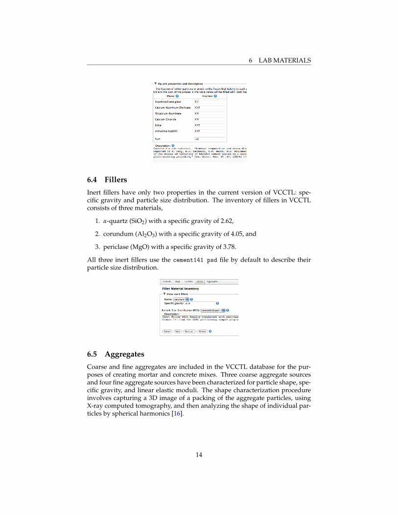
6.4 Fillers

Inert fillers have only two properties in the current version of VCCTL: spe-cific gravity and particle size distribution. The inventory of fillers in VCCTLconsists of three materials,

1. α-quartz (SiO2) with a specific gravity of 2.62,

2. corundum (Al2O3) with a specific gravity of 4.05, and

3. periclase (MgO) with a specific gravity of 3.78.

All three inert fillers use the cement141 psd file by default to describe theirparticle size distribution.

6.5 Aggregates

Coarse and fine aggregates are included in the VCCTL database for the pur-poses of creating mortar and concrete mixes. Three coarse aggregate sourcesand four fine aggregate sources have been characterized for particle shape, spe-cific gravity, and linear elastic moduli. The shape characterization procedureinvolves capturing a 3D image of a packing of the aggregate particles, usingX-ray computed tomography, and then analyzing the shape of individual par-ticles by spherical harmonics [16].

14

6 LAB MATERIALS

The aggregate materials inventory consists of one section for coarse aggre-gates and one for fine aggregates. Both sections are collapsed when the pagefirst appears and can be opened by clicking on the small grey triangle next tothe respective headings. Each section is identical except for the materials itdisplays, so the accompanying figures will illustrate the features for the fineaggregates only.

When the coarse or fine aggregate section is expanded, there is a pull-downmenu to choose which aggregate source to examine. Below that is a sectionshowing a color photograph of a small sample of the aggregate and an accom-panying table that summarizes the gross shape data for the aggregate suchas the distribution of ratios of length to width (L/W) and width to thickness(W/T) . In the table, the mean and range of L/T and W/T are provided, andbelow that a table showing the distribution of particles with given L/T andW/T. These data come from the spherical harmonic analysis, but it is useful toremember that the spherical harmonic data in the database contain much moreinformation about particle shape, enough to reproduce the 3D shape of a givenparticle of any size and rotational orientation in space.

Below the image and shape data, some physical properties of the aggregateare displayed, including the specific gravity, bulk modulus (in GPa) and shearmodulus (in GPa). Any of these properties can be changed by the user andsaved for the given aggregate (Save button) or saved as a different aggregatesource (Save As button). Finally, a text box displays other information aboutthe aggregate, including a descriptive name, the source and intended use ofthe aggregate and, in some cases, the basic mineralogical content.

Uploading entirely new aggregate sources, including all the shape data andstatistics, can be accomplished using the Upload data from a ZIP file field. Asimplied by the name, all the properties of the aggregate must be stored in textfiles with special names, and all the files must be compressed into a singleZIP archive to be uploaded correctly. However, the amount of data and the

15

7 MIX

formatting requirements for this feature are extensive, so those interested inusing this feature are encouraged to contact the author for instructions on howto prepare the archive for uploading.

7 Mix

With some knowledge of the types of materials and their properties that arestored in the VCCTL database, we turn now to the part of the software thatenables one to create mixes and cure them. This part of the software is accessedthrough the Mix tab on the main menu bar, and has a submenu for accessingtwo pages, one for creating a mix and one for simulating its hydration.

7.1 A Note on the Operating Principles of VCCTL Programs

An understanding of the underlying operating principles of VCCTL’s microstru-cure models will clarify the meaning of some of the parameters and options onthese pages. VCCTL models are based on a digital-image representation of 3Dmicrostructure. That is, microstructures are mapped onto a regular 3D grid ofcubic volume elements, often called pixels or voxels. For cement pastes, eachvoxel is 1 µm on a side, but for larger scale packings of fine or coarse aggre-gates the voxel size depends on the smallest particle that will be placed. Whena cement paste microstructure is created on this voxel grid, each voxel is oc-cupied by exactly one phase (e.g., C3S, slag, saturated porosity, etc.). In thisway, the programs that lie behind the VCCTL user interface are able to accu-rately reproduce microstructures that capture the desired phase assemblage,water/cement ratio, particle size and shape distribution, and surface areas.

Simulating hydration of these initial microstructures involves rule-basedinteractions among the voxels in the microstructure. The rules are designedto mimic the various chemical reactions and mass transport that occur duringhydration. As a result, the 3D digital image microstructure is incrementallychanged to simulate microstructure development. This process introduces newhydration product phases such as C–S–H gel, CH, ettringite, and several oth-ers.

The full details of the operating principles for the digital image approachcan be found in other publications [1, 2]. A discussion of computational toolsthat have been developed to analyze the properties of digital image microstruc-tures can be found in Ref. [18]. Some of the artifacts and limitations of digitalimage approaches are described in Ref. [17].

7.2 Prepare Mix

This page is used to create an initial 3D cement microstructure consisting ofparticles of cement clinker, calcium sulfate carriers, and other selected com-pounds in water, as well as simulated packings of fine and coarse aggregates

16

7 MIX

when the paste is acting as the binder in a mortar or concrete. There are threemain steps involved in creating the mix:

1. specifying the solid cementitious binder properties,

2. specifying the mix proportions of the solid portion of the binder withwater and aggregate, and

3. specifying the system size and other miscellaneous simulation parame-ters.

Specifying the solid cementitious binder

The principal component of the binder is one of the portland cements, whichmay be selected from among those in the database using the pull-down menuselector. Once the cement is selected, the volume fractions and surface areafractions of the clinker minerals may be modified for the mix if desired by ex-panding the section Modify phase distribution of the clinker. The default valuesdisplayed in the tables are those stored in the database for the correspond-ing cement when it was characterized as already described. The table keepsa running sum of the two columns, which should both add to 1.0. If the usermodifies the values in the columns in such a way that one or both columnsdo not sum to 1.0, the columns will be re-normalized to 1.0 when the mix iscreated.

The chosen cement also has default values for the mass fractions of the cal-cium sulfate carriers (dihydrate, hemihydrate, and anhydrite) which can bereviewed and modified by expanding the section headed Modify calcium sul-fate amounts in the cement. Remember that the displayed values are given ona total solid cement basis, and that all values are displayed as fractions, notpercentages.

The last part of specifying the solid binder is to select the type and quan-tity of any supplementary cementitious materials (SCMs) or fillers. The cate-gories for these materials are (1) fly ash, (2) slag, (3) inert filler, (4) silica fume,(4) limestone (CaCO3), and (5) free lime (CaO). For fly ash, slag, and inert filler,the materials may be selected from the accompanying pull-down menu selec-tor from those available in the database, as already described in Section 6. Forsilica fume, limestone, and free lime, the composition and specific gravity are

17

7 MIX

assumed fixed, and the user is asked only to specify the particle size distribu-tion by selecting the file for the PSD from one of those in the database. Recallthat the PSDs associated with each file can be viewed on the Lab Materials pageas described in Section 6.1. Once the material and characteristics are selected,the user may specify either the mass fraction or volume fraction that the ma-terial will occupy on a total solid binder basis. This is equivalent to specifyinga replacement level for each component. Note that the total fraction of cementin the binder is reduced as the fractions of these other materials is increased.If the mass fraction is specified, then the volume fraction will be automaticallycalculated and displayed based on the specific gravities of all the components.Similarly, specifying the volume fraction will cause the mass fraction to be au-tomatically calculated and displayed.

Specifying the mix proportions

When the solid portion of the binder is specified, the next section can be usedto specify the water/binder mass ratio (w/b) using the pull-down menu se-lector. The options for the w/b value cover the range that is normally usedfor concrete and also include the value 0.485, the latter of which is used forASTM C109 mortar cube compressive strength specimens. Text fields are alsoavailable for viewing the mass fractions and volume fractions of solid binderand water correponding to the selected w/b ratio. Modifying either a volumefraction or a mass fraction will automatically update the other fields.

This section also includes the option to add coarse or fine aggregate to themix to create a mortar or concrete. To add aggregate, click on the checkboxnext to the coarse or fine aggregate. When this is done, the text boxes for themass fraction and volume fraction, initially disabled, are enabled and the usercan type in the desired mass fraction or volume fraction, on a total mortar orconcrete basis.

In addition, when one of the aggregate checkboxes is selected, a new sectionappears below it, intially collapsed, called Change properties. Expanding this

18

7 MIX

section enables the user to specify the aggregate source, specific gravity, andgrading (or size distribution).

Notice that changing the specific gravity of the aggregate causes the volumefractions of the aggregate, binder, and water all to change in response. Finally,aggregate grading is displayed in tabular form using the customary sieve des-ignations to indicate the size bins that are used. The user may specify the grad-ing by typing in the mass fraction of aggregate retained in each sieve. The sumof the mass fractions in the table should be 1.0, but it will be normalized to 1.0if not. VCCTL comes with one pre-selected fine aggregate grading that corre-sponds to the grading specified in the ASTM C 109 mortar cube compressivestrength test. The coarse aggregate section also comes with a default aggregategrading, but the default grading does not correspond to any particular test.

Note: The aggregate grading specified manually by the user can be savedin the database for easy retrieval in subsequent mixes.

Specifying simulation parameters

After the mix proportions are specified, the user may optionally select or mod-ify any of several simulation parameters.

Random number generator seed: When the virtual microstructures are created,random numbers are used to randomly select the positions of particles as theyare added, to stochastically distribute the clinker phases within the constraintsof the two-point correlation functions, and a variety of other tasks. The randomnumber generator used in the VCCTL programs require an initial value, calleda “seed” which must be a negative integer. Under ordinary circumstances, theseed value will be chosen automatically, but the user may also specify a partic-ular seed value, if desired, by checking the box and typing any integer otherthan zero in the text box; a value of zero will cause VCCTL to automaticallygenerate a non-zero pseudo-random integer as the seed.

19

7 MIX

Real particle shapes: Check this box if you want the cement particles in the mi-crostructure to have realistic shapes. As already described, the 3D shapes of ag-gregate particles have been characterized by spherical harmonic analysis andstored in the VCCTL database to recreate realistic aggregate packings. A nearlyidentical procedure has been used to characterize the particle shapes of severaldifferent portland cement powders, except that X-ray microtomography is re-quired to obtain sufficient spatial resolution to characterize the particles usingspherical harmonics [20]. Realistic cement particle shapes will be placed in themicrostructure by marking the check box and selecting the shape set from thepull-down menu selector. Note that requesting realistic particle shapes willrequire significantly more time to create the microstructure, sometimes twoor three times as long. If the real particle shape checkbox is not selected, allthe cement particles will all be digitized spheres. Even if real particle shapesare requested, fly ash particles will remain spherical to be consistent with theirusual morphology.

Flocculation: Choosing this option will cause the particles placed in the box tobe displaced in random directions, locking with any other particles with whichthey come in contact during the process. The degree of flocculation is the frac-tion of particles that you wish to have connected into a single agglomerate.A value of 0.0 will cause no flocculation, whereas a value of 1.0 will ensurethat every particle in the system is attached to a single agglomerated structure.Intermediate values between 0 and 1 will cause a number of disconnected ag-glomerates to form, with the number of agglomerates decreasing, and theiraverage size increasing, as the degree of flocculation approaches 1.0.

Dispersion: Checking this box will ensure that every particle is separated fromevery other particle in the system by a distance of one or two voxels, therebysimulating the influence of a strong dispersing agent.

System size for the binder: The number of voxels in each linear dimension ofthe 3D grid can be chosen by the user, the default value being 100 in eachdirection. As already mentioned, each cubic voxel in the cement paste is 1 ?mon a side, so the number of voxels in each dimension is numerically equal to thelinear dimension. Note that larger values of the linear dimensions will requiresignificantly more time to create the microstructure; the time required to createa microstructure scales linearly with the number of voxels (Ncp) in the grid,which can be calculated according to the equation

Ncp = Nx NyNz

20

7 MIX

where Nx, Ny, and Nz are the numbers of voxels in the cement paste in the x,y, and z directions of the grid.

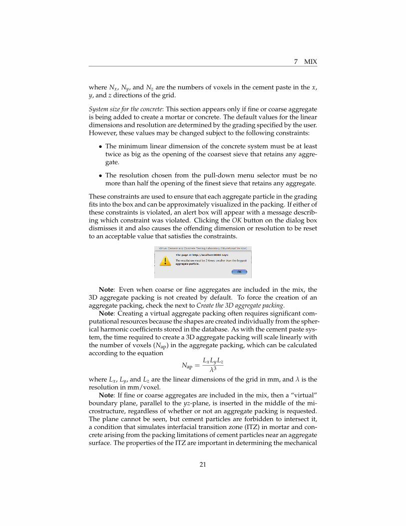
System size for the concrete: This section appears only if fine or coarse aggregateis being added to create a mortar or concrete. The default values for the lineardimensions and resolution are determined by the grading specified by the user.However, these values may be changed subject to the following constraints:

• The minimum linear dimension of the concrete system must be at leasttwice as big as the opening of the coarsest sieve that retains any aggre-gate.

• The resolution chosen from the pull-down menu selector must be nomore than half the opening of the finest sieve that retains any aggregate.

These constraints are used to ensure that each aggregate particle in the gradingfits into the box and can be approximately visualized in the packing. If either ofthese constraints is violated, an alert box will appear with a message describ-ing which constraint was violated. Clicking the OK button on the dialog boxdismisses it and also causes the offending dimension or resolution to be resetto an acceptable value that satisfies the constraints.

Note: Even when coarse or fine aggregates are included in the mix, the3D aggregate packing is not created by default. To force the creation of anaggregate packing, check the next to Create the 3D aggregate packing.

Note: Creating a virtual aggregate packing often requires significant com-putational resources because the shapes are created individually from the spher-ical harmonic coefficients stored in the database. As with the cement paste sys-tem, the time required to create a 3D aggregate packing will scale linearly withthe number of voxels (Nap) in the aggregate packing, which can be calculatedaccording to the equation

Nap =LxLyLz

λ3

where Lx, Ly, and Lz are the linear dimensions of the grid in mm, and λ is theresolution in mm/voxel.

Note: If fine or coarse aggregates are included in the mix, then a “virtual”boundary plane, parallel to the yz-plane, is inserted in the middle of the mi-crostructure, regardless of whether or not an aggregate packing is requested.The plane cannot be seen, but cement particles are forbidden to intersect it,a condition that simulates interfacial transition zone (ITZ) in mortar and con-crete arising from the packing limitations of cement particles near an aggregatesurface. The properties of the ITZ are important in determining the mechanical

21

7 MIX

properties and transport properties of mortar and concrete [6], so it is impor-tant that the ITZ be recreated in the virtual cement paste microstructure so thatits properties can be subsequently computed and incorporated into calcula-tions of mortar and concrete properties.

Saving the mix

The last steps in creating a mix are to give the mix a unique name (i.e. onethat does not already exist in the database) and execute the mix creation pro-gram. Type a name for the mix in the text box provided. Names can includeupper case or lower case letters, numbers, or spaces. After typing the proposedname and clicking anywhere outside the text box, the software will validate thename. A green checkmark (") next to the name indicates that it is valid.

A red X (%) indicates that the name has already been used for an existing mix.

Once a valid name has been chosen, click on the Create the mix button tobegin creating the mix. The status of the mix operation can be checked on theMy Operations page, as described in detail in Section 9.

7.3 Hydrate Mix

The NIST cement hydration model [1, 2] operates directly on 3D digital im-ages of cement particle microstructures created as described earlier. Executionof the model requires a starting microstructure, information about the curingconditions (thermal conditions and moisture state), and the frequency at whichto output various data for later analysis.

To begin hydrating a mix, first select the mix name from the pull-downmenu selector. This is the name chosen when the mix was created. You mayalso specify the apparent activation energies of the three major net hydrationprocesses that can occur, which are (1) cement hydration, (2) pozzolanic reac-tions, including fly ash hydration and silica fume reactions, and (3) slag hydra-tion. The default values that are provided reflect sensible values based on asurvey of the literature (for example, see ASTM C 1074). The section for mod-ifying the activation energies is collapsed when the page first opens, but maybe expanded by clicking on the small grey triangle next to the heading Reactionactivation energies.

22

7 MIX

Thermal conditions

The thermal condition of the hydrating material may be (1) isothermal, (2) semi-adiabatic, or (3) adiabatic.

Isothermal: The material is in diathermal contact with a constant-temperaturereservoir and heat transfer is sufficiently rapid to maintain the material at thetemperature of the reservoir. The default value is 25 ◦C.

Semi-adiabatic: Heat generated by hydration reactions is transferred to a sur-rounding reservoir that is at a fixed temperature, but the transfer rate is slowenough that some of the generated heat causes the material temperature to in-crease. If this option is selected, then not only the initial temperature of thematerial must be specified (default 25 ◦C), but also the temperature of the sur-rounding reservoir (default 25 ◦C) and the effective heat transfer coefficient, inunits of W/K (default 0.0, which is the adiabatic condition).

If the material being hydrated is a mortar or concrete, a section will bepresent to specify the aggregate’s initial temperature and its heat transfer coef-ficient with the binder. This feature can be useful to simulate the influence ofchilled aggregate on a hot day. However, the feature has no effect if isothermalconditions are chosen.

Adiabatic: The material is perfectly insulated from its environment, so all theheat generated by hydration reactions is used to increase the temperature ofthe material. If this option is chosen, only the initial temperature of the materialmust be specified. The default value is again 25 ◦C.

23

7 MIX

Hydration time

This section is used to specify the total length of time that the material shouldbe hydrated. The time is specified by entering the desired number of daysin the text box provided or, alternatively, by specifying a maximum degree ofhydration at which the simulation will terminate.

The other required element is the time conversion factor. The NIST hydrationmodel proceeds in repeated cycles, each of which has a dissolution step, adiffusion step to transport dissolved components through the solution, anda reaction step. These cycles have no intrinsic time scale, so one must define anassumed relationship between time (in hours) and computational cycles. In thecurrent version of VCCTL, hydration time (t) in hours is related to the numberof computational cycles (n), according to the parabolic relation

t = βn2

where β is the time conversion factor that must be specified, in units of h/cycle2.The default value of 3.5× 10−4 works reasonably well for a number of cementsbut is not optimized to any particular cement. To optimize the time conversionfactor, a calibration of the simulation against some experimental measure ofthe degree of hydration, chemical shrinkage, or isothermal heat release shouldbe made.

Note: The parabolic relation employed for the time scale is not used forany fundamental reason, but only because it often provides a reasonable fit toexperimental measurements of the progress of hydration with time, providedthat the time conversion factor has been calibrated adequately.

Note: The choice of time conversion factor has no influence on the calcula-tions other than to dilate or contract the time scale for the simulation.

Using experimental data to simulate kinetics

Cement hydration kinetics at early times can be calibrated directly using ex-perimental data as an alternative to the time conversion factor. If the cementpaste has been characterized by continuous chemical shrinkage measurementsat any isothermal temperature at or near the desired curing temperature4, theuser can upload the relevant experimental data in the appropriate format onthe Lab Materials page, check the appropriate radio button in this section, andselect the appropriate data file from the pull-down menu. See Section 6.1 forfurther details about importing experimental data.

4The temperature at which the experimental data were obtained must be isothermal and shouldbe within ±20 ◦C of the desired curing temperature, or else VCCTL’s method of using an Arrheniuscorrection to the temperature may become less accurate.

24

7 MIX

If one of these options is chosen, the VCCTL model will track the simulatedprogress of hydration in terms of the simulated chemical shrinkage or the heatsignature, and will make comparison to the available experimental data to de-termine elapsed time for any degree of hydration. If the simulation reaches atime beyond which the experimental data terminate, the models will attempt aquadratic extrapolation to later times.

Saturation conditions

The two moisture condition options are saturated or sealed. The saturatedcondition means that the cement paste is in contact with a reservoir of excesswater. As free water in the capillary pores is consumed by the hydration reac-tions, it is immediately replaced by water from the reservoir. Note, however,that once the capillary porosity reaches its percolation threshold and becomesdisconnected, water replacement is no longer possible even under saturatedconditions. The sealed condition means that free water consumed during hy-dration is not replaced. Instead, the capillary pores are progressively emptiedof water, starting in those pore regions with the largest effective diameters.

Simulation parameters

This section is collapsed when the page first opens because it will not usuallybe of interest. It can be expanded by clicking on the small grey triangle next tothe heading. The only simulation parameter that can be modified in VCCTL isthe value of the seed for the random number generator.

Data output

This section is collapsed when the page first opens. It can be expanded byclicking on the small grey triangle next to the heading. This section can be usedto specify how frequently (in hours of simulated age) the hydration model willoutput certain properties to data files.

Evaluate percolation of porosity: Percolation properties like this one tend to con-sume significant computational time to calculate because the calculations in-volve nested iterations over most or all of the system voxels. Therefore, it is rec-ommended that percolation properties not be evaluated any more often thannecessary. The percolation state of the capillary porosity determines the pointat which water can no longer be absorbed from an external source to maintainsaturated conditions. Once the hydration model detects that the pore space isdepercolated, this calculation will no longer be made no matter what value istyped into the text box. The default value is 1.0 h.

25

8 MEASUREMENTS

Evaluate percolation of total solids: This property provides an indication of initialsetting time, so it should be evaluated fairly frequently to obtain a reasonableassessment of setting time of a material. The default value is 0.5 h.

Output hydrating microstructure: The state of the entire 3D microstructure canbe saved at regular intervals during the hydration process. Subsequent calcu-lations of the linear elastic moduli, compressive strength, and transport prop-erties of the material at a particular state of hydration can only be made if themicrostructure is available at that state. The default value is 72.0 h.

Output hydration movie: If this box is checked, the model will output the mi-crostructural state of a 2D slice at time intervals specified by the user. Thesedata are then used to create a movie of the progress of hydration that can beviewed on the My Files page. Note that the default time interval of 0.0 h willresult in no movie being created. See Section 10.2 for more information aboutthe available options when viewing images and movies.

Executing the hydration simulation

To execute the simulated hydration operation, provide a unique name for theoperation in the box next to File name at the bottom of the page. The defaultname is the name of the mix with the prefix HydrationOf- prepended. Thedefault name can be modified, but must be unique. The software validates thename before and will indicate a green " (okay) or a red % (invalid) next tothe name. Once a valid name is selected, click on the Hydrate the mix button tolaunch the operation. The status of the hydration operation can be checked onthe My Operations page, as described in detail in Section 9.

Note: One or more hydration operations for a particular mix can be re-quested and launched even before the mix operation has been completed. Ifthe mix operation is still running when the hydration request is made, a mes-sage will appear saying, The mix you want to hydrate is not ready now. The hy-dration will begin as soon as the mix preparation is finished. In other words, thehydration operation is queued to run as soon as the mix operation completesand a starting microstructure is available.

8 Measurements

In VCCTL, 63 properties are continuously tracked during a hydration opera-tion, and all of them are stored in a data file that can be accessed for onlineplotting or exporting to a spreadsheet for further analysis. See Appendix C for

26

8 MEASUREMENTS

a listing of all the available hydrated properties. In addition, the linear elas-tic moduli, compressive strength and transport properties of cement pastes,mortars, or concretes can be calculated on hydrated microstructures. The Mea-surements page provides access to all these virtual measurement capabilities.

Clicking on the Measurements tab of the main menu bar opens a page with asubmenu having two options: (1) Plot Hydrated Properties, and (2) MeasureCement/Concrete Properties.

8.1 Plot Hydrated Properties

This page provides a flexible inline plotting capability for plotting the evolvingproperties of a hydrating material. To create a plot, first select the desired prop-erty to use for the x-axis from the pull-down menu selector. The default x-axisis Time, in hours, but any other hydrated property can be selected as well.

With the x-axis selected, any number of properties can be simultaneously plot-ted on the y-axis, including multiple properties from a single hydration simu-lation, or a comparison of the same properties for different hydration simula-tions. To create a plot, first select a hydration operation on the left pull-downmenu selector (under the heading Hydration Name), and then select the desiredproperty to plot in the right pull-down menu selector (under the heading Prop-erty). Doing so will immediately create the plot in the Plot result area.

27

8 MEASUREMENTS

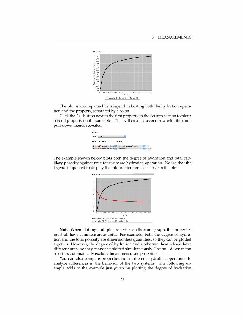
The plot is accompanied by a legend indicating both the hydration opera-tion and the property, separated by a colon.

Click the “+” button next to the first property in the Set axes section to plot asecond property on the same plot. This will create a second row with the samepull-down menus repeated.

The example shown below plots both the degree of hydration and total cap-illary porosity against time for the same hydration operation. Notice that thelegend is updated to display the information for each curve in the plot.

Note: When plotting multiple properties on the same graph, the propertiesmust all have commensurate units. For example, both the degree of hydra-tion and the total porosity are dimensionless quantities, so they can be plottedtogether. However, the degree of hydration and isothermal heat release havedifferent units, so they cannot be plotted simultaneously. The pull-down menuselectors automatically exclude incommensurate properties.

You can also compare properties from different hydration operations toanalyze differences in the behavior of the two systems. The following ex-ample adds to the example just given by plotting the degree of hydration

28

8 MEASUREMENTS

for another hydration operation. Notice that the second hydration operation,HydrationOf-ASTMC109-02, only ran for 24 h.

Plotted curves can be removed from the graph by clicking on the “-” buttonnext to the corresponding row in the Set axes section.

Note: Under some conditions, the generated plot may not automaticallyrescale its axes in an optimal way. This can be corrected by simply clickingonce anywhere within the region of the plot itself.

It is also possible to zoom in on a narrow range of the x-axis. To do so,place the mouse within the plot field at the beginning x value. Hold the mousebutton down and drag to the ending x value. Releasing the mouse will auto-matically generate the rescaled plot. Again, to go back to the optimal scalingneeded to show all the data, just click once within the plot region.

Finally, a high-resolution plot can be created in separate pop-up window byclicking on the High resolution version link below the legend. The same zoomingfeatures apply to the high-resolution plot as for the regular plot.

Note: When a hydration operation is running, its progress can be moni-tored by going to this plotting page. The default plot, which has time on thex-axis, will show how much simulation time has been reached, even if the op-eration has not completed.

8.2 Measure Cement/Concrete Properties

Clicking on this subtab opens a page for calculating the linear elastic proper-ties, compressive strength, and the effective diffusivity of cement pastes, mor-tars, or concretes that have been hydrated. The desired hydration operationcan be chosen from the pull-down menu selector. When this is done, a listingof the available hydration times for this operation appears under the headingProperties.

29

8 MEASUREMENTS

Recall that, when a hydration operation is requested, you have the optionto select the time intervals at which to output the partially hydrated 3D mi-crostructures. For example, if you chose 72.0 h for this interval, microstructureswere saved at approximately 72 h, 144 h, 216 h, etc. These are the same timesthat now appear in the list on this page, as individually collapsed sections, anyof which can be expanded by clicking on the small grey triangles next to theheadings.

When one of these individual sections is expanded, it reveals two buttons, oneto calculate the elastic properties (effective linear elastic moduli) and one tocalculate the transport properties (relative diffusivity and formation factor).Clicking on these buttons launches the finite element models that calculatethese properties on the digital image [15].

The finite element calculations take significant computational time to com-plete, about 20 min to 30 min for a typical 100 × 100 × 100 system. Once thecalculations begin, the relevant section of this page will display several boxesthat will eventually contain the results of the calculations. While the calcula-tions are ongoing, however, these boxes will display the message Measuring . . . .The data that are displayed in these boxes when the calculations are completedis described now.

30

8 MEASUREMENTS

Elastic properties results

There are three text boxes to display the elastic properties results:

• The first box provides a summary of the effective elastic properties ofthe cement paste, including the bulk modulus, K in GPa, shear modu-lus, G in GPa, Young’s modulus, E in GPa, and Poisson ratio, ν. If thematerial is a mortar or concrete, this box will also display the effectiveelastic properties of the mortar or concrete. These latter properties arecalculated with Differential Effective Medium Theory (D-EMT) [19], andinclude the effective K, G, E, and ν. The D-EMT model takes the cementpaste elastic properties, aggregate elastic properties, and the properties ofthe ITZ (also gleaned from the finite element calculations on the cementpaste near the aggregate surface, as described below), as well as the vol-ume fractions of the paste, aggregates, and air voids. In addition to theseproperties, a mortar or concrete will also have the estimated compressivestrength displayed in the box, in MPa, which is estimated from the em-pirical relationship between Young’s Modulus and compressive strengthdescribed by Neville [21].

• The second box shows the relative contribution to the elastic propertiesof each phase in the microstructure. For each phase in turn, the followingdata are provided

1. the volume fraction of the phase2. the mean value, over all the voxels of the given phase, of the bulk

modulus calculated using the linear elastic relation between the lo-cal stress and the macroscopically applied strain

3. the fraction that this value is of the total effective bulk modulus ofthe material

4. the mean value (defined as in (2)) of the shear modulus5. the fraction that this value of shear modulus is of the total effective

shear modulus

31

8 MEASUREMENTS

6. the mean value (defined as in (2)) of Young’s modulus

7. the fraction that this value of Young’s modulus is of the total effec-tive Young’s modulus

• The third box contains information about the variation of the elastic prop-erties of the cement paste as a function of distance perpendicular to theaggregate surface. The data appear in five columns, identified as

1. distance from the aggregate surface (µm)

2. K for the paste (GPa)

3. G for the paste (GPa)

4. E for the paste (GPa)

5. ν for the paste.

These data are calculated directly from the finite element model results andare used to determine the elastic properties of the ITZ. The ITZ properties aredetermined by averaging these data over thickness of the ITZ, which is approx-imately equal to the median particle size of the starting cement powder [6].

Transport properties results

Calculated transport properties are displayed in one box, and consist of therelative diffusion coefficient in the x, y, and z directions. Here the relative dif-fusion coefficient is defined as the effective diffusion coefficient of mobile so-lution species in the material, divided by the diffusion coefficient of the samespecies in pure pore solution having the same composition. In addition, theaverage relative diffusion coefficient over all three dimensions and the forma-tion factor are displayed in the text box. The formation factor is the inverse ofthe average relative diffusion coefficient as defined here.

Following the value of the formation factor, the text box displays phase-specific information similar to that displayed for elastic properties above. Foreach phase in turn, the following data are provided:

• the volume fraction of the phase

• the relative conductivity of the phase, that is, the conductivity of mobilespecies through the phase itself divided by the conductivity of the samespecies through pure pore solution of the same composition; saturated

32

9 MY OPERATIONS

porosity has a relative conductivity of 1.0 by definition, and solid densephases have a relative conductivity of 0.0

• the fraction that this phase contributes to the overall effective conductiv-ity of the composite materials in each orthogonal direction.

9 My Operations

The My Operations page is the central location for checking the status of a user’soperations. This guide has already discussed all of the major operations thatcan be executed in VCCTL, but now is a good time to list all the types in sum-mary.

• Microstructure: Creation of a cement paste microstructure

• Aggregate: Creation of a mortar or concrete aggregate packing

• Hydration: Simulating the hydration of a cement paste

• Elastic-moduli: Calculation of elastic moduli of a cement paste, mortar, orconcrete

• Transport-factor: Calculation of relative diffusion coefficients and forma-tion factor

On the My Operations page, each operation for a user is listed in one of foursections, depending on their status: queued, running, finished, or cancelled.

9.1 Queued Operations

When an operation is requested on one of the VCCTL pages, it is given an entryin the database and is placed in a queue waiting to be run. Some operationswill leave the queue and begin running almost immediately, but some others,such as hydration operations waiting for their microstructure to be created,will remain in the queue for some time. While in the queue, a new directory iscreated to store the results, and an input file is created for the C program thatwill process the input and generate the results. On the My Operations page,operations in the queue appear in a yellow table at the top of the page, withinformation about the type of operation (see the previously enumerated list fortypes) and the time of the request displayed.

33

9 MY OPERATIONS

At the right of the entry is a link to delete the operation from the queue. Click-ing the Delete link will remove the operation request from the database anddelete the directory associated with that operation.

9.2 Running Operations

While an operation is running, it appears in a green table in this section. Thename of the operation appears as a link. If the name is clicked, the My Filespage is opened to the operation in question so the user can examine the filesthat have been generated for the operation. See Section 10 for more detail onthe My Files page. In addition to the name, the operation type and the timestarted are displayed.

At the right of the entry is a link to cancel the operation. Clicking the Cancellink will terminate the C program that is running the operation, and the oper-ation will be moved to the Cancelled operations section of the page. The inputand output files associated with the operation will remain intact, and any datagenerated up to the point of cancellation can be viewed on the My Files page.

9.3 Finished Operations

When the C program running an operation has finished (either successfully orunsuccessfully), the operation is moved from the Running operations section tothis section. It appears as an entry in a blue table. As before, the name of theoperation appears as a link that redirects the page to the operation’s entry inthe My Files page. In addition to the name, the operation type is displayed, aswell as the time the operation started and finished.

At the right of each entry is a link to delete the finished operation. Clickingthe Delete link will delete all input and output files generated by the operationand will remove the operation’s listing from the database.

Note: The deletion of an operation cannot be undone, so use this featurewith caution.

34

10 MY FILES

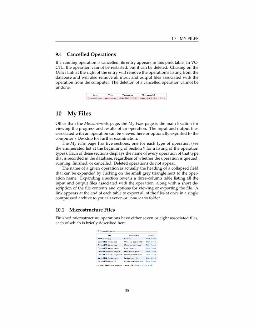
9.4 Cancelled Operations

If a running operation is cancelled, its entry appears in this pink table. In VC-CTL, the operation cannot be restarted, but it can be deleted. Clicking on theDelete link at the right of the entry will remove the operation’s listing from thedatabase and will also remove all input and output files associated with theoperation from the computer. The deletion of a cancelled operation cannot beundone.

10 My Files

Other than the Measurements page, the My Files page is the main location forviewing the progress and results of an operation. The input and output filesassociated with an operation can be viewed here or optionally exported to thecomputer’s Desktop for further examination.

The My Files page has five sections, one for each type of operation (seethe enumerated list at the beginning of Section 9 for a listing of the operationtypes). Each of these sections displays the name of every operation of that typethat is recorded in the database, regardless of whether the operation is queued,running, finished, or cancelled. Deleted operations do not appear.

The name of a given operation is actually the heading of a collapsed fieldthat can be expanded by clicking on the small grey triangle next to the oper-ation name. Expanding a section reveals a three-column table listing all theinput and output files associated with the operation, along with a short de-scription of the file contents and options for viewing or exporting the file. Alink appears at the end of each table to export all of the files at once in a singlecompressed archive to your Desktop or Downloads folder.

10.1 Microstructure Files

Finished microstructure operations have either seven or eight associated files,each of which is briefly described here.

35

10 MY FILES

Grading: A text file containing the aggregate grading specified when creating amortar or concrete. This entry will not be present for cement pastes. The con-tents of this file, and any other simple text file, can be displayed in a scrollingtext box by clicking on the Show link at the right of the entry. It consists of threecolumns:

1. the common name of the sieve

2. the sieve opening size (in mm)

3. the mass fraction of aggregate retained in the sieve

The text box can be hidden again by clicking on the Hide link. Again, this orany other file on the My Files page can be exported to the Desktop or Downloadsfolder by clicking on the Export link.

One-pixel bias numbers: Cement paste microstructures in VCCTL have a reso-lution of 1 µm, but a large number of cement particles are smaller than thisminimum feature size. To include these particles in the virtual microstruc-ture, they are represented as 1 µm clusters of smaller particles. These clustersshould have a higher surface area and, consequently, a greater rate of reactionwith water than a single particle of the same size. The one-pixel bias numbers,calculated from knowledge of the cement particle size distribution in the sub-micrometer range, are included in this file as a triplet of numbers, one numberon each row, for each phase in the initial microstructure. The triplet is format-ted as follows:

• The first number in the triplet is always 0, for reasons having to do withthe legacy versions of the software.

• The second number in the triplet is the bias value, a decimal numbertypically near 1.0, but which may be significantly greater than 1.0 for finecements, or slightly less than 1.0 for coarse cements.

• The third number in the triplet is the integer identification number of thephase. Appendix B lists the identification numbers for the phases.

Microstructure image: This file contains a listing of the phase occupying eachvoxel in the 3D virtual microstructure. The file has a five-line header withself-descriptive entries, followed by the integer phase identification numberfor each voxel in the grid, with one voxel per row. Ordinarily, the text version

36

10 MY FILES

of this file will hold little interest to the user. Therefore, clicking on the Showlink will cause a thumbnail color image of a 2D slice from the microstructureto display. Please refer to Section 10.2 for more information on working withthese images.

Input to genmic: This is the input file read by the C program (genmic) that cre-ates the virtual microstructure. It is difficult to read because it is not annotatedin any way. More sense can be made of the input file by viewing it in conjunc-tion with the output file, the latter which provides a running commentary onthe types of input being read.

Output from genmic: This is the output file produced by the C program (gen-mic) as it runs. This file ordinarily will be of little interest, but it can provideimportant clues to the cause of any failure of the program to execute properly.If genmic fails for some reason, an error message will typically appear near theend of the output file.

Particle SH coefficients: A listing of the coefficients in the spherical harmonic(SH) expansion describing the shape of each particle in the microstructure. Thisfile probably is of no interest to most users.

Particle image file: This file is a complement to the microstructure image file.Whereas the microstructure image associates a unique phase identification num-ber to each voxel, the particle image file associates a particle number to eachvoxel. Specifically, a voxel is assigned a number n if the phase at that voxel be-longs to the nth particle in the microstructure. Porosity is assigned the numberzero, and particles comprised of only one voxel also are assigned zero. Thisfile is used internally by the C program responsible for hydration operations(disrealnew) and should hold no interest for most users.

Cement phase statistics: A tabular display of the number of voxels assigned toeach phase in the final microstructure, along with the corresponding mass frac-tion, volume fraction, and surface area fraction of that phase in the virtual mi-crostructure. This file consists of two sections. The first eight lines of the filedisplay the phase statistics on a total clinker solid basis. This section can beused to determine how closely the final microstructure reproduces the clinkerphase fractions and w/b ratio that were requested when the operation waslaunched. The remaining part of the file lists four values for each phase, in thisorder:

1. number of voxels assigned to that phase

2. number of voxel faces of that phase that are adjacent to porosity; this isthe digitized analog of the surface area.

3. volume fraction of the phase in the microstructure, on a total volumebasis (solids plus porosity)

37

10 MY FILES

4. mass fraction of the phase in the microstructure, on a total mass basis(solids plus porosity)

10.2 Displaying microstructure images

As already described, microstructure images are displayed as color 2D slices ofthe 3D microstructure. VCCTL provides the ability to view the microstructureat different magnifications and from different perspectives, so we now devoteattention to explaining these features.

Clicking on the Show link for any microstructure image file displays a thumb-nail image of a 2D cross section from the 3D virtual microstructure. Note thatit may take several seconds for this image to display because it is being createdat the time of the Show request.

The thumbnail is a color image, with each color corresponding to a differentphase in the mix. Once the thumbnail is displayed, it can be clicked with themouse to open another page for more detailed examination and manipulationof the image.

38

10 MY FILES

Plane to view: Choose one of three orthogonal directions from which to viewthe microstructure. The viewing planes are defined by the two Cartesian coor-dinate axes they contain (e.g., the yz-plane is the plane observed when viewingalong the x-axis).

Slice to view: Changing this value enables the user to view the image at differentlocations along the axis of viewing. Valid values are in the interval [0, Lx − 1],where Lx is the number of voxels in the direction being viewed. Values outsidethe valid interval are converted to the nearest value in the valid interval. Forexample, a slice value of -7 would be converted to 0.

Magnification: A positive integer value of M displays the image with a squareof M × M image pixels corresponding to each voxel in the original image slice.Note: the magnification value must be a positive integer.

Depth Perception: Selecting yes from the pull-down menu will reveal the mi-crostructure just below the surface of the current slice, much as if the porositywere filled with a murky liquid.

39

10 MY FILES

Backscattered Electron Contrast: Selecting yes from the pull-down menu will dis-play a gray-scale image of the microstructure in which the relative brightnessof each phase corresponds approximately to what would be observed in abackscattered electron image of a polished section using a scanning electronmicroscope.

Once the viewing options are selected, click the Get image button or justpress the Enter key on the keyboard to view the new image. Images previouslyviewed while this page has been open can be accessed by clicking the Backbutton on your browser.

Underneath the displayed image is a key showing the colors assigned toeach phase in the microstructure. The color key is identical to that used toview cements on the Lab Materials page, described in Section 6.1.

10.3 Aggregate Files

Finished aggregate packing operations have seven associated files, each of whichis briefly described here.

40

10 MY FILES

Input to genaggpack: This is the input file read by the C program (genaggpack)that creates the virtual microstructure. It is difficult to read because it is notannotated in any way. More sense can be made of the input file by viewing itin conjunction with the output file, the latter which provides a running com-mentary on the types of input being read.

Output from genaggpack: This is the output file produced by the C program(genaggpack) as it runs, especially describing the nature of the input valuesthat are read. Note: Ordinarily, the output file will be of little interest, butit can provide important clues to the cause of any failure of the program toexecute properly. If genaggpack fails for some reason, an error message willtypically appear near the end of the output file.

Microstructure image: This file contains a listing of the phase occupying eachvoxel in the 3D virtual microstructure. In contrast to cement paste microstruc-tures, an aggregate packing has either two or three phases present. Porosityand aggregate are always present. In addition, if the resolution of the pack-ing is sufficiently fine that the ITZ can be resolved, it will appear as a separatephase for easy visualization. Clicking on the Show link will cause a thumbnailcolor image of a 2D slice from the microstructure to display. Please refer toSection 10.2 for more information on working with these images.

Particle SH coefficients: A listing of the coefficients in the spherical harmonic(SH) expansion describing the shape of each particle in the packing. This file isof no interest to most users.

Phase statistics: A tabular display of the number of voxels assigned to eachphase in the final packing. There is one line for porosity, one line for aggregate,and one line for ITZ. A value of zero for ITZ does not mean that there is noITZ in the mortar or concrete, but instead means that the virtual packing wascreated at too coarse a resolution to include the ITZ in the image.

Besides these five files, a oneimage.input file and a oneimage.output fileare also present in the table. These are used in the auxiliary program to renderthe aggregate packing image, and are of no interest to VCCTL users.

10.4 Hydration Files

Finished hydration operations often have a dozen or more associated files.

41

10 MY FILES

Cement alkali characteristics: Contains information on both the total and thereadily-soluble potassium and sodium in the cement. The format and view-ing of this file were discussed in Section 6.1.

Fly ash alkali characteristics: This file is required even if the material does notcontain any fly ash. Its format is identical to that for the cement alkali charac-teristics file.

Hydration image: There will likely be ten or more of this type of file in the list.Each one is a saved 3D microstructure at a different time during hydration. Theactual number of this type of file depends on the time interval that was speci-fied between successive outputs and on the total simulated time. For example,if a user requests hydration for 28 d (672 h) with microstructure output every72 h, there will be 10 hydration images (72 h, 144 h, 216 h, 288 h, 360 h, 432 h,504 h, 576 h, 648 h, and a final microstructure at 672 h when the run finishes).All but the final hydration image files have the following pattern for its name:

MicrostructureName.img.xxx.xxh.TT.0yz

where

• MicrostructureName is the name given to the initial microstructure (i.e.,the microstructure operation name).

• xxx.xxh is the number of hours (to the nearest 0.01 h) of hydration towhich this image corresponds. Note: The exact time at which the mi-crostructure is output is as close to the desired time interval as possible,but the elapsed time of each hydration cycle is not constant and so outputat the exact time interval requested is rarely possible.

• TT is the initial temperature used for the hydration operation (◦C).

• y is 0 if isothermal conditions were specified, or is 1 if adiabatic or semi-adiabatic conditions were specified.

42

10 MY FILES

• z is 0 if hydrating under saturated conditions, or is 1 if hydrating undersealed conditions.

As an example, a hydrated image name of MyMic.img.289.20h.25.000 meansthe original microstructure is named MyMic.img, the microstructure was outputat 289.20 h of hydration time, the initial temperature was 25 ◦C, and isothermaland saturated conditions were used.

The exception to this naming pattern is the final image that is written whenthe hydration operation terminates. This final image has the pattern

HydrationName.img.TT.0yz

where HydrationName is the name of the hydration operation, and TT, y, and z

have the same meaning as before.Clicking the Show link for any of the hydration images will cause a thumb-

nail color image of a 2D slice from the microstructure to display. Please refer toSection 10.2 for more information on working with these images.

Hydration movie: A file of this type (with extension .mov) will be present if andonly if the relevant option was selected when the hydration simulation waslaunched. Clicking the Show link will display a thumbnail animation of theprogress of hydration of a 2D slice from the microstructure. Clicking on thethumbnail will produce a larger image that can be viewed at different magni-fications and different viewing speeds.

Pore size distribution: A file with extension poredist is created with every im-age file. Clicking on the Show link will display a bar chart representation ofthe capillary pore size distribution of the simulated microstructure, plotted asa differential distribution. Unlike images, the thumbnail image cannot be ex-panded and manipulated.

Input to disrealnew: This is the input file read by the C program (disrealnew)that performs the virtual hydration operation. It is difficult to read because itis not annotated in any way. More sense can be made of the input file by view-ing it in conjunction with the output file, the latter which provides a runningcommentary on the types of input being read.

Output from disrealnew: This is the output file produced by the C program(disrealnew) as it runs, especially describing the nature of the input valuesthat are read. Note: Ordinarily, the output file will be of little interest, but it canprovide important clues to the cause of any failure of the program to executeproperly. If disrealnew fails for some reason, an error message will typicallyappear near the end of the output file.

Image index.txt: This is a two-column text file. The left column gives the timesat which the hydration images were output, and the right column contains thefull path name to the hydration image in question. Ordinarily, this file will beof no interest to most users, because any or all the images can be exported tothe Desktop or Downloads folder by clicking on the Export link.

43

10 MY FILES

Parameters file: A listing of the several dozen parameters used by the C program(disrealnew) in its execution. These parameters cannot be modified by theuser.

Slag characteristics: Contains information about the physical and chemical char-acteristics of the slag, and the slag hydration products, used in the microstruc-ture. This file must be input to the hydration operation even if no slag is presentin the microstructure. The format and viewing of this file were discussed inSection 6.2.

Hydration results: A large tabular display of the values of the 63 hydration prop-erties at each computational cycle. This file has 63 columns and several hun-dred rows, making it difficult to view in the small text box that is providedwhen the Show button is clicked. It is much more convenient to export thefile and then import it into a spreadsheet application. Also, recall that anyone or more of the properties in this file can be simultaneously plotted on theMeasurements page of VCCTL. The meaning of each of the 63 columns in thehydration results file is provided in Appendix C.

10.5 Mechanical Properties Files

Finished mechanical properties operations have five associated files, each ofwhich is briefly described here.

Input to elastic: This is the input file read by the C program (elastic) thatperforms both the finite element calculations of the effective elastic moduli ofcement paste and, for mortar or concrete, the effective medium theory calcula-tions of the effective moduli and compressive strength of the material. This filehas only a few lines, but it is not easy to understand because it is not annotated.More sense can be made of the input file by viewing it in conjunction with theoutput file, the latter which provides a running commentary on the types ofinput being read.

Output from elastic: This is the output file produced by the C program (elastic)as it runs, especially describing the nature of the input values that are read.Note: Ordinarily, the output file will be of little interest, but it can provideimportant clues to the cause of any failure of the program to execute properly.If elastic fails for some reason, an error message will typically appear near theend of the output file.

44

10 MY FILES

Effective moduli results: This file is displayed in the first text box on the Mea-surements page when a mechanical property operation is finished. Its formatis described in Section 8.2.

Phase contributions: This file is displayed in the second text box on the Mea-surements page when a mechanical property operation is finished. Its formatis described in Section 8.2.

ITZ elastic characteristics: This file is present only if aggregate has been includedin the mix (i.e., only for a mortar or concrete). It is displayed in the third text boxon the Measurements page when a mechanical property operation is finished.Its format is described in Section 8.2.

10.6 Transport Properties Files

Finished transport properties operations have four associated files, each ofwhich is briefly described here.

Phase contributions: This file is displayed in the second text box on the Mea-surements page when a transport property operation is finished. Its format isdescribed in Section 8.2.

Input to transport: This is the input file read by the C program (dc3d) that per-forms both the finite difference calculations of the effective relative diffusioncoefficients and formation factor of the given microstructure image. This filehas only a few lines, but it is not easy to understand because it is not annotated.More sense can be made of the input file by viewing it in conjunction with theoutput file, the latter which provides a running commentary on the types ofinput being read.

Output from transport: This is the output file produced by the C program (dc3d)as it runs, especially describing the nature of the input values that are read.Note: Ordinarily, the output file will be of little interest, but it can provideimportant clues to the cause of any failure of the program to execute properly.If dc3d fails for some reason, an error message will typically appear near theend of the output file.

Major transport output data: This file contains rather verbose output from thedc3d program, including the status of the conjugate gradient relaxation method[Garboczi98] at the end of each iteration. Ordinarily, this file will hold no inter-est for the user.

45

11 LOGOUT

Transport factor results: This file is displayed in the first text box on the Mea-surements page when a transport property operation is finished. Its format isdescribed in Section 8.2.

11 Logout

To gracefully log out of the VCCTL system, click on the Logout tab in the mainmenu bar. This logs you out immediately and also takes you to the originallogin page for the system, where you can switch to a new user.

Note: If you wish to shut down VCCTL and close the browser, as explainedin Section 3, you must also

• wait for all running operations to finish, or cancel all running operations,

• close the web browser, and then

• open the Java console window and press Ctrl-C. After a brief pause, youwill be asked, Terminate batch job (Y/N)?. Type y and press the Enter but-ton. The Java console window will close.

46

A PREPARING AND UPLOADING NEW CEMENT DATA

Appendices

A Preparing and Uploading New Cement Data

VCCTL comes packaged with an executable file called processImageJ.exe

that can be run from the command line to package the data for a new cementinto the kinds of data files that ultimately will be needed to create the zippedarchive needed to upload the cement into VCCTL. This program is designedto take just the segmented and indexed image file and create nearly all the filesnecessary to upload a cement into VCCTL 9. The program runs from the com-mand line in an interactive way, prompting the user for responses that it needsto create the text files.

A.1 Getting Ready

1. Make sure that the processImageJ.exe executable file is somewhere inyour PATH environment, or else be prepared to type in the full path nameto it when you want to run it.

2. You must have ImageMagick installed on your computer. It can be down-loaded freely at

http://www.imagemagick.org/script/binary-releases.php#windows

Just download and run the executable from the website to begin the in-stallation, and choose all the defaults during the installation.

3. Create a folder and put your segmented, indexed image file in the folder.Note: the indexed image file must have the extension .txt.

4. For the purposes of these instructions, we will call the folder NewCement,and we will call the image file NewCementIndexedImage.txt.

5. Decide the name you want this cement to have in VCCTL. For the pur-poses of these instructions, we will use the name MyNewCement

6. To make the best use of this program, you should have the following dataready when you run it, because the program will prompt you for thesedata. You don’t need to have them, but you will have to go back andmodify the individual files later if not.

(a) The spatial resolution of the image, in units of µm/pixel. This isimportant because it sets the scale for all the correlation functionkernels that will get created. Prior experience indicates that an in-correct scaling will not dramatically affect VCCTL results, but it canaffect the fidelity with which VCCTL microstructures will mimic thereal microstructure.

47

A PREPARING AND UPLOADING NEW CEMENT DATA

(b) The mass fraction (not percentage) of gypsum, hemihydrate, andanhydrite in the cement, on a total solids basis.

(c) Na2O % by mass

(d) K2O % by mass

(e) Readily soluble Na2O % by mass (less than or equal to total Na2O %by mass)

(f) Readily soluble K2O % by mass (less than or equal to total K2O %by mass)

(g) Percent of total Na2O added as NaOH to mix water (usually zero)

(h) Percent of total K2O added as NaOH to mix water (usually zero)

(i) A descriptive name for the cement (several words)

(j) Several words describing the source of the cement.

(k) Several words indicating the date when cement was characterized(e.g., April 2014)

(l) Surface area of the cement, in units of m2/kg

(m) How the surface area was measured (e.g., Blaine, BET, particle sizedistribution)

(n) Knowledge of the indexing of the image (i.e., which phase is associ-ated with which index in the image file).

A.2 Running processImageJ

1. Drag the NewCement folder to your Desktop.

2. Open a command window.

3. Type cd Desktop\NewCement.

4. Type FULL_PATH_TO_VCCTL_FOLDER\bin\processImageJ.exe and pressEnter, where FULL_PATH_TO_VCCTL_FOLDER is the location of the VCCTLinstall folder

5. Answer each of the questions in turn, based on the information com-piled in the previous section. The necessary files will be created in theNewCement directory.

A.3 What To Do Next

1. If you have the cement particle size distribution in the acceptable format,give it the same root name as all the other newly created files in theNewCement folder, using the extension .psd, and place it in the NewCementdirectory. The correct format is an ASCII text files with two columnsseparated by either a tab or space:

48

A PREPARING AND UPLOADING NEW CEMENT DATA

(a) The particle diameter in µm units

(b) The differential mass fraction (not percent) for each size.

If you don’t have the particle size distribution ready, you can add it laterwithin the VCCTL software.

2. Optionally, if you have quantitative X-ray diffraction data available inASCII text form (format is unimportant, usually some kind of tabularformat), give it the same root name as all the other newly created files,using the extension .xrd, and place it in the NewCement directory with theother files. If you don’t have the particle size distribution ready, you canadd it later within the VCCTL software.

3. Collect all the newly created files in a single zip archive.

4. When you’re ready, you can upload this zip file on the Lab Materials pageof VCCTL.

5. After the upload has completed, the segmented image may not appear,but the other fields on the Lab Materials page should be updated as ex-pected. Make sure to save the cement using the Save As button, and givethe cement the same name as the root name of all the files created byprocessImageJ.

6. The image of the cement should also appear the next time you visit thepage and examine the new cement.

49

B INTEGER ID NUMBERS OF VCCTL PHASES

B Integer ID Numbers of VCCTL Phases

This appendix gives the integer identification number and the short displayname that is used in VCCTL for each phase that is recognized in the system.

Phase Name Display Name IDSaturated porosity POROSITY 0C3S (alite) C3S 1C2S (belite) C2S 2C3A (cubic form) C3A 3C4AF C4AF 4K2SO4 (arcanite) K2SO4 5Na2SO4 (thenardite) NA2SO4 6Gypsum (CaSO4 · 2H2O) GYPSUM 7Bassanite (CaSO4 · 0.5H2O) HEMIHYD 8Anhydrite (CaSO4) ANHYDRITE 9Silica fume SFUME 10Inert filler INERT 11Slag SLAG 12Aggregate INERTAGG 13Aluminosilicate glass in fly ash ASG 14Calcium aluminosilicate glass in fly ash CAS2 15Amorphous silica AMSIL 16C3A in fly ash FAC3A 17Portlandite (CH) CH 19C–S–H gel CSH 20Hydrogarnet (C3AH6) C3AH6 21AFt (generic ettringite) ETTR 22AFt with Fe substitution ETTRC4AF 23AFm (generic monosulfate) AFM 24Fe(OH)3 FH3 25C–S–H gel with low Ca/Si POZZCSH 26C–S–H from slag reactions SLAGCSH 27CaCl2 CACL2 28Friedel’s salt (C3A·CaCl2 · 10H2O) FRIEDEL 29Stratlingite (C2ASH8) STRAT 30Secondary gypsum GYPSUMS 31CaCO3 (generic limestone) CACO3 33Calcium monocarboaluminate AFMC 34Brucite (Mg(OH)2) BRUCITE 35MgSO4 MS 36Free lime (CaO) FREELIME 37C3A (orthorhombic form) OC3A 38Dried porosity DRIEDP 53Self-desiccated porosity EMPTYP 55

50

C CONTENTS OF HYDRATION RESULTS FILE

C Contents of Hydration Results File

This appendix provides a brief description of each column in the hydrationresults file (ending in .data; see Section 10.4 for more information).

Column Heading Description1 Cycle computational cycle2 time(h) hydration time (h)3 Alpha mass degree of hydration on a cement mass ba-

sis4 Alpha fa mass degree of hydration of fly ash on a fly ash

mass basis5 Heat(kJ/kg solid) heat liberated (> 0 for exothermic, kJ/kg

of solids)6 Temperature(C) system temperature (◦C)7 Gsratio paste gel-space ratio (see [22])8 Wno(g/g) non-evaporable water (g water/ g ce-

ment) on an unignited cement mass basis9 Wni(g/g) non-evaporable water content (g water/

g cement) on an ignited cement mass10 ChemShrink(mL/g) chemical shrinkage (mL/g of cement)11 pH estimated pH of the capillary pore solu-

tion12 Conductivity estimated DC conductivity of the pore

solution (S/m)13 [Na+](M) estimated Na+ in solution (mol/L)14 [K+](M) estimated K+ in solution (mol/L)15 [Ca++](M) estimated Ca2+ in solution (mol/L)16 [SO4--](M) estimated SO2−

4 in solution (mol/L)17 {K+} estimated molal activity of K+ in solution18 {Ca++} estimated molal activity of Ca2+ in solu-

tion19 {OH-} estimated molal activity of OH− in solu-

tion20 {SO4--} estimated molal activity of SO2−

4 in solu-tion

21 Vfpore Volume fraction of capillary pores

51

C CONTENTS OF HYDRATION RESULTS FILE

Column Heading Description22 Poreconnx Fraction of capillary pore volume that forms a

percolated network in the x direction23 Poreconny Fraction of capillary pore volume that forms a

percolated network in the y direction24 Poreconnz Fraction of capillary pore volume that forms a

percolated network in the z direction25 Poreconnave Arithmetic mean of columns 22–2426 Solidconnx Fraction of solids that form a percolated network

in the x direction27 Solidconny Fraction of solids that form a percolated network

in the y direction28 Solidconnz Fraction of solids that form a percolated network

in the z direction29 Solidconnave Arithmetic mean of the columns 26–28

30–63 Vfxxx Volume fraction of phase xxx on a system volumebasis, where xxx is the display name of the phasegiven in Appendix I.

52

REFERENCES

References

[1] Dale P. Bentz. Three-dimensional computer simulation of cement hydra-tion and microstructure development. J. Am. Ceram. Soc., 80(1):3–21, 1997.1, 7.1, 7.3

[2] Dale P. Bentz. CEMHYD3D: A three-dimensional cement hydrationand microstructure development modeling package. Version 3.0. NI-STIR 7232, U.S. Department of Commerce, June 2005. Available athttp://ciks.cbt.nist.gov/monograph. 1, 7.1, 7.3

[3] Dale P. Bentz and J. T. Conway. Computer modeling of the replacementof ‘coarse’ cement particles by inert fillers in low w/c ratio concretes: Hy-dration and strength. Cem. Concr. Res., 31:503–506, 2002. 1

[4] Dale P. Bentz, X. Feng, Claus J. Haecker, and Paul E. Stutzman. Analysisof CCRL proficiency cements 135 and 136 using CEMHYD3D. NISTIR6545, U.S. Department of Commerce, August 2000. Available online at theNIST electronic monograph, http://ciks.cbt.nist.gov/monograph, Part I,Chapter 4, Section 3. 1

[5] Dale P. Bentz and Edward J. Garboczi. Simulation studies of the effects ofmineral admixtures on the cement paste-aggregate interfacial zone. ACIMater. J., 88:518–529, 1991. 1

[6] Dale P. Bentz and Edward J. Garboczi. Computer modelling of interfa-cial transition zone microstructure and properties. In M. G. Alexander,G. Arliguie, G. Ballivy, A. Bentur, and J. Marchand, editors, Engineeringand Transport Properties of the Interfacial Transition Zone in Cementitious Com-posites, pages 349–385. RILEM, Paris, FRANCE, 1999. 7.2, 8.2

[7] Dale P. Bentz, Edward J. Garboczi, Claus J. Haecker, and Ole M. Jensen.Effects of cement particle size distribution on performance properties ofcement-based materials. Cem. Concr. Res., 29(10):1663–1671, 1999. 1

[8] Dale P. Bentz and Claus J. Haecker. An argument for using coarse cementsin high performance concretes. Cem. Concr. Res., 29:615–618, 1999. 1

[9] Dale P. Bentz, Ole M. Jensen, K. K. Hansen, J. F. Olesen, H. Stang, andClaus J. Haecker. Influence of cement particle size distribution on earlyage autogenous strains and stresses in cement-based materials. J. Am.Ceram. Soc., 84(1):129–135, 2000. 1

[10] Dale P. Bentz and Paul E. Stutzman. SEM analysis and computer mod-elling of hydration of Portland cement particles. In S. M. DeHayes andD. Stark, editors, Petrography of Cementitious Materials, pages 60–73. Amer-ican Society for Testing and Materials, Philadelphia, PA, 1994. 6.1

53

REFERENCES

[11] Dale P. Bentz, Paul E. Stutzman, Claus J. Haecker, and S. Remond.SEM/X-ray imaging of cement-based materials. In H. S. Pietersen, J. A.Larbia, and H. H. A. Janssen, editors, Proceedings of the 7th Euroseminar onMicroscopy Applied to building Materials, pages 457–466. Delft University ofTechnology, 1999. 6.1

[12] Jeffrey W. Bullard and Edward J. Garboczi. A model investigation of theinfluence of particle shape on portland cement hydration. Cem. Concr. Res.,36(6):1007–1015, 2006. 1

[13] Jeffrey W. Bullard and Paul E. Stutzman. Analysis of CCRL Portland ce-ment proficiency samples number 151 and number 152 using the virtualcement and concrete reference laboratory. Cem. Concr. Res., 36:1548–1555,2006. 1

[14] X. Feng, Edward J. Garboczi, Dale P. Bentz, Paul E. Stutzman, andThomas O. Mason. Estimation of the degree of hydration of blended ce-ment pastes by a scanning electron microscope point-counting procedure.Cem. Concr. Res., 34(10):1787–1793, 2004. 6.3

[15] Edward J. Garboczi. Finite element and finite difference programs forcomputing the linear electric and elastic properties of digital images ofrandom materials. NISTIR 6269, U.S. Department of Commerce, Decem-ber 1998. 1, 8.2

[16] Edward J. Garboczi. Three-dimensional mathematical analysis of particleshape using X-ray tomography and spherical harmonics: Application toaggregates used in concrete. Cem. Concr. Res., 32(10):1621–1638, 2002. 6.5

[17] Edward J. Garboczi and Dale P. Bentz. The effect of statistical fluctuation,finite size error, and digital resolution on the phase percolation and trans-port properties of the NIST cement hydration model. Cem. Concr. Res.,31:1501–1514, 2001. 7.1

[18] Edward J. Garboczi, Dale P. Bentz, and Nicos S. Martys. Digital imagesand computer modelling. In P-z. Wong, editor, Methods in the Physics ofPorous Media, number 35 in Experimental methods in the Physical Sci-ences, pages 1–41. Academic Press, San Diego, CA, 1999. 7.1

[19] Edward J. Garboczi and James G. Berryman. Elastic moduli of a mate-rial containing composite inclusions: Effective medium theory and finiteelement computations. Mech. Mater., 3e:455–470, 2001. 8.2

[20] Edward J. Garboczi and Jeffrey W. Bullard. Shape analysis of a referencecement. Cem. Concr. Res., 34:1933–1937, 2004. 7.2

[21] A. M. Neville. Properties of Concrete. Prentice-Hall, Harlow, England, 1995.8.2

54

REFERENCES

[22] Hal F. W. Taylor. Cement Chemistry. Thomas Telford, London, secondedition, 1997. C

55