
CODED MEASUREMENT FOR IMAGING AND SPECTROSCOPY
120
CODED MEASUREMENT FOR IMAGING AND SPECTROSCOPY by Andrew David Portnoy Department of Electrical and Computer Engineering Duke University Date: Approved: David J. Brady, Supervisor Jungsang Kim David Smith Xiaobai Sun Rebecca Willett Dissertation submitted in partial fulfillment of the requirements for the degree of Doctor of Philosophy in the Department of Electrical and Computer Engineering in the Graduate School of Duke University 2009
Transcript of CODED MEASUREMENT FOR IMAGING AND SPECTROSCOPY

CODED MEASUREMENT FOR IMAGING AND
SPECTROSCOPY
by
Andrew David Portnoy
Department of Electrical and Computer EngineeringDuke University
Date:Approved:
David J. Brady, Supervisor
Jungsang Kim
David Smith
Xiaobai Sun
Rebecca Willett
Dissertation submitted in partial fulfillment of therequirements for the degree of Doctor of Philosophy
in the Department of Electrical and Computer Engineeringin the Graduate School of
Duke University
2009

ABSTRACT
CODED MEASUREMENT FOR IMAGING AND
SPECTROSCOPY
by
Andrew David Portnoy
Department of Electrical and Computer EngineeringDuke University
Date:Approved:
David J. Brady, Supervisor
Jungsang Kim
David Smith
Xiaobai Sun
Rebecca Willett
An abstract of a dissertation submitted in partial fulfillment of therequirements for the degree of Doctor of Philosophy
in the Department of Electrical and Computer Engineeringin the Graduate School of
Duke University
2009

Copyright c© 2009 by Andrew David Portnoy
All rights reserved

Abstract
This thesis describes three computational optical systems and their underlying coding
strategies. These codes are useful in a variety of optical imaging and spectroscopic
applications. Two multichannel cameras are described. They both use a lenslet array
to generate multiple copies of a scene on the detector. Digital processing combines the
measured data into a single image. The visible system uses focal plane coding, and
the long wave infrared (LWIR) system uses shift coding. With proper calibration, the
multichannel interpolation results recover contrast for targets at frequencies beyond
the aliasing limit of the individual subimages. This theses also describes a LWIR
imaging system that simultaneously measures four wavelength channels each with
narrow bandwidth. In this system, lenses, aperture masks, and dispersive optics
implement a spatially varying spectral code.
iv

Acknowledgements
The PhD process takes persistence. This has been a long journey, one that I have not
traveled alone. Throughout my life, I have been fortunate to have great teachers, and
I would not be here today if it were not for them. I wish to take this opportunity to
thank everyone who has supported me along the way. My parents, Michael and Susan
Portnoy, and my sister, Elizabeth Portnoy, have always given me encouragement, and
I will always love them.
Dr. David Brady, has been a wonderful advisor, and his insight has truly shaped
this research. He and the other faculty at Duke University have provided an out-
standing environment to grow and discover. Much inspiration has also come from
Dr. Kristina Johnson, who remains an outstanding mentor. I would like to thank my
committee members, Dr. Jungsang Kim, Dr. David Smith, Dr. Xiaobai Sun, and
Dr. Rebecca Willett, for their time and feedback throughout this process.
I want to thank the past and present members of DISP with whom I have formed
fruitful collaborations and friendships. Thank you to Dr. Nikos Pitsianis, Dr. Bob
Guenther, Dr. Mohan Shankar, Steve Feller, Dr. Scott McCain, Dr. Michael Gehm,
Dr. Evan Cull, Christina Fernandez Cull, Dr. John Burchett, Ashwin Wagadarikar,
Sehoon Lim, Paul Vosburgh, David Kittle, Nan Zheng, Dr. Yangqia Wang, Dr.
Qi Hao, Dr. Unnikrishnan Gopinathan, and Dr. Jungpeng Guo. International
collaborators Dr. Ken Hsu, Dr. Jason Fang, Satoru Irie, and Ryoichi Horisaki have
helped me to see to the world. For both research and unrelated discussions, I also
wish to extend thanks to fellow Duke graduate students including Dr. Vito Mecca,
Kenny Morton, Dr. Josh Stohl, William Lee, Neera Desai, and Zac Harmany.
For their support in administration and logistics, I thank Wendy Lesesne, Jennifer
Dubow, Justin Bonaparte, Leah Goldsmith, Tasha Dawson, Ellen Currin, Samantha
v

Morton, Kristen Rogers, and Steve Ellis. WCPE Classical Radio always provides a
relaxing voice. For their support to build CIEMAS, I thank, in particular, Michael
and Patty Fitzpatrick, James Frey, and the Yoh Family. For their support to fund
this research, I thank Dr. Dennis Healy, Dr. Ravi Athale, and Dr. Philip Perconti.
Lastly, I want to write a special acknowledgement to my dear friend, Greg Chion,
who lost his 9-month battle with leukemia on October 26, 2000 our senior year of
high school. Greg was everything from a fellow Cub Scout to a fellow drum major,
and it is in his memory that this thesis is dedicated. Having such wonderful friends
and family, I know that throughout my life, I will Never Walk Alone.
vi

In memory of Greg Chion
vii

Contents
Abstract iv
Acknowledgements v
List of Tables xi
List of Figures xii
1 Introduction 1
1.1 Computational Imaging . . . . . . . . . . . . . . . . . . . . . . . . . 1
1.2 Motivation . . . . . . . . . . . . . . . . . . . . . . . . . . . . . . . . . 3
1.3 Organization . . . . . . . . . . . . . . . . . . . . . . . . . . . . . . . 4
2 Focal Plane Coding 6
2.1 Background . . . . . . . . . . . . . . . . . . . . . . . . . . . . . . . . 6
2.2 Multichannel Imaging System Analysis . . . . . . . . . . . . . . . . . 7
2.2.1 System Model . . . . . . . . . . . . . . . . . . . . . . . . . . . 8
2.2.2 Lenslet displacements . . . . . . . . . . . . . . . . . . . . . . . 9
2.2.3 Focal Plane Masks . . . . . . . . . . . . . . . . . . . . . . . . 11
2.2.4 Decoding analysis . . . . . . . . . . . . . . . . . . . . . . . . . 13
2.3 System Implementation . . . . . . . . . . . . . . . . . . . . . . . . . . 17
2.3.1 Focal Plane Array . . . . . . . . . . . . . . . . . . . . . . . . . 18
2.3.2 Lenslet Array . . . . . . . . . . . . . . . . . . . . . . . . . . . 19
2.3.3 Focal Plane Coding Element . . . . . . . . . . . . . . . . . . . 21
2.3.4 Lens Alignment . . . . . . . . . . . . . . . . . . . . . . . . . . 21
2.4 Impulse Response Measurement . . . . . . . . . . . . . . . . . . . . . 24
viii

2.5 Single Image Construction . . . . . . . . . . . . . . . . . . . . . . . . 28
2.6 Discussion . . . . . . . . . . . . . . . . . . . . . . . . . . . . . . . . . 32
3 Multichannel Shift Coding 35
3.1 Introduction . . . . . . . . . . . . . . . . . . . . . . . . . . . . . . . . 35
3.2 System Transfer Function and Noise . . . . . . . . . . . . . . . . . . 38
3.3 Optical Design and Experimental System . . . . . . . . . . . . . . . . 44
3.4 Image Reconstruction . . . . . . . . . . . . . . . . . . . . . . . . . . . 48
3.4.1 Registration . . . . . . . . . . . . . . . . . . . . . . . . . . . . 48
3.4.2 Reconstruction . . . . . . . . . . . . . . . . . . . . . . . . . . 48
3.4.3 Results . . . . . . . . . . . . . . . . . . . . . . . . . . . . . . . 52
3.5 Experimental Results . . . . . . . . . . . . . . . . . . . . . . . . . . . 55
3.5.1 Noise Equivalent Temperature Difference . . . . . . . . . . . . 55
3.5.2 Spatial Frequency Response . . . . . . . . . . . . . . . . . . . 58
3.6 Conclusion . . . . . . . . . . . . . . . . . . . . . . . . . . . . . . . . . 64
4 Multichannel Narrow Band Spatiospectral Coding 66
4.1 Introduction . . . . . . . . . . . . . . . . . . . . . . . . . . . . . . . . 66
4.2 Elementary Example . . . . . . . . . . . . . . . . . . . . . . . . . . . 68
4.2.1 Direct measurement of individual wavelength channels . . . . 71
4.3 System Architecture . . . . . . . . . . . . . . . . . . . . . . . . . . . 73
4.4 Mathematical Model . . . . . . . . . . . . . . . . . . . . . . . . . . . 75
4.5 System Implementation and Components . . . . . . . . . . . . . . . . 77
4.5.1 Camera and Lenses . . . . . . . . . . . . . . . . . . . . . . . . 77
4.5.2 Mask Design . . . . . . . . . . . . . . . . . . . . . . . . . . . . 78
4.5.3 Prism Design . . . . . . . . . . . . . . . . . . . . . . . . . . . 79
ix

4.5.4 Mechanical Design . . . . . . . . . . . . . . . . . . . . . . . . 80
4.6 Calibration . . . . . . . . . . . . . . . . . . . . . . . . . . . . . . . . 81
4.6.1 Noise Equivalent Temperature Difference . . . . . . . . . . . . 81
4.6.2 Monochromator Calibration . . . . . . . . . . . . . . . . . . . 81
4.6.3 Prism Characterization . . . . . . . . . . . . . . . . . . . . . . 84
4.6.4 Spectral Impulse Response Measurements . . . . . . . . . . . 86
4.6.5 Wide Field Calibration . . . . . . . . . . . . . . . . . . . . . . 91
4.7 Results . . . . . . . . . . . . . . . . . . . . . . . . . . . . . . . . . . . 93
5 Conclusions 97
6 APPENDIX A 99
Bibliography 101
Biography 104
x

List of Tables
2.1 Condition numbers for the decoding process associated with the mod-ified Hadamard coding on K ×K lenslet arrays . . . . . . . . . . . . 17
2.2 The condition numbers associated with P × P partition of N × Ndetector arrays. . . . . . . . . . . . . . . . . . . . . . . . . . . . . . . 17
3.1 Experimentally calculated contrast, V , for 4 bar targets at 5 spatialfrequencies. . . . . . . . . . . . . . . . . . . . . . . . . . . . . . . . . 64
4.1 Narrow band filters used to calibrate the monochromator. . . . . . . . 84
xi

List of Figures
1.1 Raw data from a computational imaging system . . . . . . . . . . . . 2
2.1 The focal plane coding masks. . . . . . . . . . . . . . . . . . . . . . . 12
2.2 Photographs of the COMP-I Focal Plane Coding Camera. . . . . . . 18
2.3 Magnified image of CMOS pixels. . . . . . . . . . . . . . . . . . . . . 19
2.4 The unmounted refractive lenslet array. . . . . . . . . . . . . . . . . . 20
2.5 Microscope image of the imaging sensor with a focal plane coding element 22
2.6 The focal plane coding element under 100X magnification . . . . . . . 22
2.7 Impulse response scan of four adjacent pixels . . . . . . . . . . . . . . 26
2.8 Coded Impulse Response Scan . . . . . . . . . . . . . . . . . . . . . . 27
2.9 2D Pixel Impulse Response . . . . . . . . . . . . . . . . . . . . . . . . 28
2.10 Masked 2D Pixel Impulse Response . . . . . . . . . . . . . . . . . . . 29
2.11 Checkerboard Masked 2D Pixel Impulse Response . . . . . . . . . . . 29
2.12 Raw captured image from focal plane coded camera . . . . . . . . . . 31
2.13 Focal Plane Coded Camera Reconstruction Comparison . . . . . . . . 32
2.14 Pixel Intensity Plot Comparison . . . . . . . . . . . . . . . . . . . . . 33
3.1 Comparison of STF . . . . . . . . . . . . . . . . . . . . . . . . . . . . 40
3.2 Wiener filter error comparison . . . . . . . . . . . . . . . . . . . . . . 43
3.3 Designed LWIR optical train . . . . . . . . . . . . . . . . . . . . . . . 45
3.4 Theoretical MTF performance of the LWIR system . . . . . . . . . . 46
xii

3.5 Diamond-turned germanium element . . . . . . . . . . . . . . . . . . 47
3.6 Photograph of LWIR cameras used . . . . . . . . . . . . . . . . . . . 47
3.7 Comparison of 3 reconstruction algorithms . . . . . . . . . . . . . . . 52
3.8 Comparison between conventional and multichannel cameras . . . . . 53
3.9 Long range LWIR comparison . . . . . . . . . . . . . . . . . . . . . . 54
3.10 Copper targets used for collimator system . . . . . . . . . . . . . . . 56
3.11 LWIR Testbed . . . . . . . . . . . . . . . . . . . . . . . . . . . . . . . 56
3.12 Signal-to-noise ratio versus temperature . . . . . . . . . . . . . . . . 57
3.13 Registered pixel responses . . . . . . . . . . . . . . . . . . . . . . . . 60
3.14 Data and interpolation for target at 0.120 cy/mrad . . . . . . . . . . 62
3.15 Intensity plot for target at 0.120 cy/mrad . . . . . . . . . . . . . . . 62
3.16 Data and interpolation for target at 0.192 cy/mrad . . . . . . . . . . 63
3.17 Intensity plot for target at 0.192 cy/mrad . . . . . . . . . . . . . . . 63
4.1 Datacube . . . . . . . . . . . . . . . . . . . . . . . . . . . . . . . . . 66
4.2 Bayer Pattern . . . . . . . . . . . . . . . . . . . . . . . . . . . . . . . 67
4.3 Datacube Transformations . . . . . . . . . . . . . . . . . . . . . . . . 70
4.4 Dual-disperser hyperspectral imaging architecture . . . . . . . . . . . 70
4.5 Direct Measurement of Color Channels . . . . . . . . . . . . . . . . . 72
4.6 Direct Measurement of Narrow band Color Channels . . . . . . . . . 74
4.7 LWIR Multispectral Camera . . . . . . . . . . . . . . . . . . . . . . . 77
4.8 Mask Details . . . . . . . . . . . . . . . . . . . . . . . . . . . . . . . 78
xiii

4.9 LWIR Prism . . . . . . . . . . . . . . . . . . . . . . . . . . . . . . . . 79
4.10 Spot Diagram . . . . . . . . . . . . . . . . . . . . . . . . . . . . . . . 80
4.11 Signal-to-noise ratio versus temperature . . . . . . . . . . . . . . . . 82
4.12 LWIR Ruled Grating Spectral Efficiency . . . . . . . . . . . . . . . . 82
4.13 LWIR Glowbar Source Operating Characteristics . . . . . . . . . . . 83
4.14 Blackbody Spectrum for 1000 oC Source . . . . . . . . . . . . . . . . 84
4.15 Monochromator with narrow band filter . . . . . . . . . . . . . . . . 85
4.16 LWIR Pixel Spectral Responses . . . . . . . . . . . . . . . . . . . . . 89
4.17 LWIR Response at Key Wavelengths . . . . . . . . . . . . . . . . . . 90
4.18 Wide Field Calibration . . . . . . . . . . . . . . . . . . . . . . . . . . 92
4.19 LWIR Datacube . . . . . . . . . . . . . . . . . . . . . . . . . . . . . 95
4.20 LWIR Datacube . . . . . . . . . . . . . . . . . . . . . . . . . . . . . 96
xiv

Chapter 1
Introduction
1.1 Computational Imaging
Photography is evolving. Digital imaging sensors replace film in an increasing num-
ber of applications, and there is no indication this trend will subside. The shift from
analog to digital facilitates new opportunities because computers can now more nat-
urally process image data. In this way, computers have essentially become consumers
of photographs. Generally speaking, the trend in machine vision has been to acquire
images pleasing to the human eye and pass them directly to the computer for pro-
cessing. This paradigm is not necessarily optimal. The source data need not look
conventional to a human for it to contain meaningful information. One example that
exploits this freedom is data compression, which enables computers to store, process,
and transmit the same information in different representations. Furthermore, image
compression algorithms (like JPEG) represent photographs in significantly fewer bits
which reduce storage and transmission demands. Even when discarding information,
computers often will display for humans images indistinguishable from their origi-
nal. Image compression algorithms allow for the tradeoff increased computational
demands with greater storage efficiency. While image compression does not concern
itself with the acquisition of image data, computational imaging systems explore the
co-design of optical systems and digital processing.
Computational imaging is the next generation of digital imaging processing. It
brings computation into the physical layer by using optical components to perform
non-trivial data processing. This is in contrast to conventional photography which
uses lenses to generate structurally identical copies of a scene on a film negative.
1

With computational optics, one can begin processing data before transducing pho-
tons into bits. A well designed system measures compressed data directly. In general,
a computational system includes both hardware (optics and sensors) and software
(algorithms). A co-design of these components enables novel hardware designs in-
cluding multichannel or multiplex architectures. Multichannel systems sample in
parallel; they measure multiple copies of a signal simultaneously. Multiplex systems
sample the superposition of multiple signals in a single measurement. In fact, the
prototype described in Chapter 2 combines both of these concepts. An example of
the raw data acquired from this computational system is shown in Figure 1.1. The
scene consists of a single soup can, and digital processing demultiplexes and com-
bines multiple channels to recover a single image. The raw data from computational
optical systems is not intended to be human readable. By design these systems rely
on digital processing to extract meaningful information.
Figure 1.1: An example of raw data acquired from the computational imaging sys-tem. This image is taken from the multichannel camera described in Chapter 2. Thesource is a single can of soup, however, multiple images are acquired simultaneously.
2

1.2 Motivation
Coding strategies are the tools of computational optical systems. They facilitate
mappings between the source field and the detector. And, a major theme of compu-
tational imaging is designing an elegant mapping. This dissertation explores coded
measurement, developing an understanding for a collection of tools which may be
used in a variety of applications. The motivation for Chapters 2 and 3 is thin digital
imaging. Both implementation utilize a multichannel design, capturing many copies
of a scene and combining them with post-processing. In this way, these techniques
extend to a broader class of applications beyond just “thin” systems. At the core of
Chapter 4 is designing a color (or multispectral) long wave infrared camera (LWIR).
In particular, one that measures multiple narrow band channels simultaneously. Color
digital cameras for the LWIR are not as readily available as they are for the visible
band.
This thesis investigates coding strategies to better understand digital sampling.
Standard focal plane arrays are used in the prototypes, however, their pixel sampling
functions are modulated. This occurs in three major ways: spatial coding (Chapter
2), coding in sampling phase (Chapter 3), and spectral response coding (Chapter
4). Additionally, this thesis develops characterization tools to measure sampling
functions.
Computational imaging system designers balance performance with instrument
and algorithmic complexity. By providing descriptions of new coding strategies, this
thesis empowers system designers with more tools. The coding principles described
in this thesis may be applied to new applications. Regardless, the characterization
tools developed are important because one can better interpret the data collected
by an instrument by better understanding its sampling functions. The instrument’s
transfer function filters the electromagnetic field when measurements are made and
3

that mechanism provides a context (or basis) for the collected data.
1.3 Organization
The focus of this dissertation is a description three different coding strategies for
optical imaging and spectroscopy systems as well as an instrument demonstrating
each one. The first is focal plane coding, a technique which directly modulates
the detector sampling functions. The second relies on subpixel shifts as a coding
mechanism. Finally, the third explores coding in wavelength.
Chapter 2 describes a thin digital imaging systems that uses a multichannel lenslet
array. Multiple copies of the scene are generated on the detector plane and are
processed to generate a single conventional image. The subpixel features on the focal
plane coding element reduces redundancy between each image by modulating pixels
differently in each region. This camera operates in the visible region.
Chapter 3 explores the design and implementation of a second multichannel cam-
era. In contrast to the system described in Chapter 2, this one operates in the Long
Wave Infrared (LWIR) band, which is also referred to as thermal imaging. Shift based
coding reduces redundancy in this instrument. The performance is also extensively
characterized and compared to that of a conventional LWIR camera.
Chapter 4 extends coding into the spectral domain. A snapshot spectral im-
ager is developed and tested operating in the LWIR. This particular implementation
measures multiple narrow spectral bands simultaneous by using image plane coding
masks in combination with dispersive elements. This marks an improvement of the
typical LWIR camera which is essentially an intensity detector because it is sensitive
to broad band light.
The final chapter of this dissertation provides some general conclusions related
to coding in imaging and spectroscopy. Some comments and observations are also
4

proposed which could further develop this evolving field.
5

Chapter 2
Focal Plane Coding
2.1 Background
The generalized sampling theory by Papoulis [1] has been applied in multiband or
multichannel imaging [2–4]. In particular, several research groups have focused on
the application of the theory to “super-resolved” optical imaging [5–8]. Previous
implementations of multichannel sampling strategies have primarily utilized optical
techniques to optimize specific system metrics. For example, multichannel sampling
with multiple aperture lenslet arrays has been used in the TOMBO 1 system [9] to
substantially reduce imaging system thickness and volume. The TOMBO system
is based on a compound-eye which uses multiple independent imaging lenses. The
images are combined digitally with post processing. Broadly, there is considerable
interest in improving or optimizing performance metrics for computational imagers
on multichannel sampling. The Compressive Optical MONTAGE Photography Ini-
tiative (COMP-I) [10–12] has explored new strategies for multichannel imagers by a
co-design of the optics, the electronic sampling strategy, and computational recon-
struction scheme [13].
This chapter describes the formal basis of the focal-plane coding strategies. It
specifically analyses and compares the TOMBO scheme and a multiplexing scheme
developed for the COMP-I system [11]. Both systems utilize thin imaging optics us-
ing a lenslet array, multiapertures and computational integration of a single higher-
resolution image from multiple images. They differ in two major ways. First, the
COMP-I system uses an additional element, a focal plane mask. Second, the system’s
1TOMBO stands for thin observation module by bound optics.
6

computational reconstruction procedures have differing complexity and stability. Be-
cause of computational resources are finite, it is an important concern to assess both
the efficiency of a particular design as well as the errors introduced from its post pro-
cessing algorithm. This chapter describes the COMP-I implementation of the coding
schemes and presents experimental results.
The next section introduces a mathematical framework for both designing focal
plane coding systems as well as comparing multichannel imaging systems. Section 2.3
details the components of the system built to demonstrated focal plane coding. The
following two sections, 2.4 and 2.5, present the experimental results and image re-
constructions obtained from the system. A discussion is provided in Section 2.6.
2.2 Multichannel Imaging System Analysis
Multichannel sampling is well understood in concept since the seminal work by Pa-
poulis [1]. This section introduces a novel realization of the multi-channel sampling
theory on optical system in order to reduce camera thickness without compromising
image resolution. The following describes a framework of multichannel sampling as
well as the algebraic procedures for decoding, i.e. constructing a single image without
the loss of resolution.
First illustrated is a description of a multichannel system implemented with lenslet
displacements only, the mechanism first demonstrated by TOBMO system [9]. Sec-
ond, a mutlichannel system using coding masks is described which is implemented
in the COMP-I system [14]. The two coding schemes have different numerical be-
haviors in computational image reconstruction. Both systems are explored under the
following unifying framework of multichannel optical imaging systems.
7

2.2.1 System Model
In a typical image system, the object field, f(x, y), is blurred by a point spread
function (PSF), which is a characteristic of the imaging system. In an ideal case, the
PSF is shift invariant and can be represented by its impulse response h(x, y). The
blurred image is electronically sampled by a two-dimensional detector array, G = [gij],
where gij is the measurement at pixel (i, j). Establishing the origin at the center of
a rectangular focal plane, let the array limits be [−X/2, X/2]× [−Y/2, Y/2]. In the
case of incoherent imaging, the transformation from the source intensity f(x, y) in
object space to the discrete data array G = [gij] measured by the detector may be
modeled as follows.
gij =
∫ X/2
−X/2
∫ Y/2
−Y/2
sij
(x, y, f(x, y)
)dxdy,
f(x, y) =
∫ ∞
−∞
∫ ∞
−∞f(ξ, η) h(αx− ξ, αy − η) dξdη,
(2.1)
where f is the blurred and scaled image at the focal plane, modeled by the convolution
of the object function with the PSF, α is a system-dependent scaling parameter which
will be illustrated shortly, and the function sij characterizes the sampling at the (i, j)
pixel of the blurred image at the focal plane. The support of sij(x, y) may be limited
to the geometry and location of the pixel at the detector.
All the pixels at the detector assume the same rectangular shape, ∆x × ∆y. In
practice, square pixels are common, ∆x = ∆y = ∆. Each pixel is uniquely identified
by its Cartesian location. Thus, the center of the (i, j) pixel is at (i∆x, j∆y), −M ≤i ≤ M , −N ≤ j ≤ N , with (2M + 1)∆x = X, (2N + 1)∆y = Y . The characteristic
8

function of the (i, j) pixel at the detector array modeled as
Pij(x, y) = rect
(x
∆x
− i
)rect
(y
∆y
− j
)(2.2)
where rect(x) = 1 if x ∈ [−1/2, 1/2] and rect(x) = 0 otherwise. The pixel function,
Pi,j, described above represents a unity fill factor pixel. In practice, this ideal function
has to be revised to describe incomplete fill factors in actual electronic pixels. In the
case there is no additional coding at the focal plane, the pixel sampling function can
be simply described by the multiplication of the pixel function and the function to
sample from,
sij(x, y, f(x, y)) = Pij(x, y) f(x, y).
With such a sampling function, the pixel at (i, j) location is said to be clear. The
following cases introduce non-trivial focal plane coding schemes used in conjunction
with multichannel imaging systems. In the general case of multiple channels, the
model in (2.1) applies to each channel individually.
2.2.2 Lenslet displacements
The TOMBO system [9] can be characterized as a special case of the system model
(2.1). It aims at reducing the thickness of the optical system by replacing a single
large aperture lens with an array of smaller aperture lenses or lenslets. The detector
pixel array is accordingly partitioned so that each and every lenslet corresponds to
a subarray. Let the image on a subarray be called a subimage, relative to the mul-
tiple copies of the scene on the entire array. In order to maintain the resolution of
the system with a single large aperture lens, a diversity in the subimages is essen-
tial. Otherwise, the detector array carries redundant, identical subimages of lower
resolution.
9

The TOMBO system exploits the relative non-uniform displacements of the lenslets
at manufacture. Consider a 3 × 3 array of lenslets. There are 9 subimages at 3 × 3
sub-apertures, Gpq = [gpq,ij], p, q = −1, 0, 1. Here, the double-indices pq associated
with G in the capital case specify the subarray or subimage corresponding to the
lenslet at location p, q; the four-tuple indices (pq, ij) associated with g in small case
specify the (i, j) pixel in the (p, q) subarray or subimage. The subimage at the center
is G00. The subimage Gpq is made different from G00 by the displacement of the (p, q)
lenslet relative to the center one.
In concept, the lenslet displacement can be designed first and calibrated after
system manufacturing. In terms of the framework in Section 2.2.1, the following
model describes a multiple channel imaging system
gpq,ij =
∫ X/2
−X/2
∫ Y/2
−Y/2
spq,ij
(x, y, f(x, y)
)dxdy,
f(x, y) = =
∫ ∞
−∞
∫ ∞
−∞f(ξ, η) h(βx− ξ, βy − η) dξdη,
(2.3)
where β is the scaling factor relating the object scene to the subapertures. The choice
β = 3α is natural for 3×3 lenslet array, where α is the scaling factor for a comparison
single entire aperture system. The sampling functions for lenslet displacements can
be described as follows,
spq,ij(x, y, f(x, y)) = Pij(x, y) Epq(f(x, y)) = Pij(x, y) f(x− δp, y − δq), (2.4)
where E denotes the shift operator. Diversity is introduced when δp and δq are not
multiples of ∆. By design, one may deliberately set δp = p δ, δq = q δ with δ = ∆/3.
A couple of remarks are in order. It is assumed that the lenslets have the identical
views of the same object at the scene. The lenslet shifting, which is non-circulant,
requires the additional knowledge or assumption on the boundary conditions in nu-
10

merical reconstruction. Subsection 2.2.4 discusses the procedures for computational
integration of the multiple images and the numerical properties of the problem. The
following subsection shows extends the sampling function of the array model described
in (2.3) to allow for the use of focal plane coding masks.
2.2.3 Focal Plane Masks
The model framework of (2.1) and (2.3) allows for various focal plane coding schemes.
Mask-based codes are introduced here, which are implemented in COMP-I program.
Each lenslet is associated with a mask representing a unique code. Consider, for
example, a 4×4 lenslet array. Figure 2.1 shows all the 16 masks, one for each lenslet,
based on the Hadamard matrix. Every channel has a unique mask, and each pixel
in that region is masked with the same code. In other words each subimage is coded
uniquely. The pixel-wise sampling function can be described as follows,
spq,ij(pq, ij)(x, y, f(x, y)) = Pij(x, y)Hpq(x, y) f(x, y), (2.5)
where the function Hpq represents the codeword implemented by the mask at the
(p, q) lenslet or channel. The first channel is clear or un-masked.
The masks, or two-dimensional codewords, are drawn from Hadamard matrices.
The masks on a 4× 4 lenslet array are constructed as follows.
Hpq =1
2
((H4 eq)(H4 eT
p ) + eeT), (2.6)
where H4 is the 4× 4 Hadamard matrix with elements in −1, 1 (see Appendix A),
ek is the k-th column of the identity matrix, e is the column vector with all elements
equal to 1. In other words, first, the outer product of the q-th column and p-th row
of H4 is formed. Then all the −1’s are replaced with 0’s. This result is shown in
11

2 4
2
4
2 4
2
4
2 4
2
4
2 4
2
4
2 4
2
4
2 4
2
4
2 4
2
4
2 4
2
4
2 4
2
4
2 4
2
4
2 4
2
4
2 4
2
4
2 4
2
4
2 4
2
4
2 4
2
4
2 4
2
4
Figure 2.1: The focal plane coding masks used for the 4× 4 lenslet array based onthe Hadamard matrix.
12

Figure 2.1, where the black sub-pixels block the light and represent zero values in
the codewords Hpq. Masks with binary patterns are relatively easy to manufacture,
and the fabricated element is described in Section 2.3. The masks have the effect of
partitioning every single pixel into 4× 4 subpixels.
The order of Hadamard matrices is limited to powers of 2. This limitation is lifted
by introducing the following 0-1 valued and well-conditioned matrices
H3 =
1 1 11 −1 11 1 −1
, H5 =
(H4 eeT −1
). (2.7)
These are the leading sub-matrices of H4 and H5, respectively.
The sampling function specified pixel-wise by (2.5) and (2.6) is well conditioned
for numerical image reconstruction. The next subsection shows that how the modified
Hadamard focal plane coding scheme is more efficient and more stable compared to
the shift based codes.
2.2.4 Decoding analysis
This subsection analyzes the decoding or integrating process, which is an important
step for computational construction of a single image at the subpixel level, compen-
sating the coarse resolution with the thin optics.
Assume the lenslet array has P × Q individual lenses. The pixel array A is
partitioned into P ×Q blocks, each block corresponding to a subimage with M ×N
pixels. Let A(p, q, i, j) specify the (i, j) element in the (p, q) subarray. Also, there is
a related array A,
A(i, j, p, q) = A(p, q, i, j). (2.8)
This form is simply a pixel rearrangement so that the (i, j) block in A is composed of
all the (i, j) pixels from the subarrays in A. While the block array A is a multiplex
13

of the subimages, A is the image indexed by channel (p, q).
If all the pixels in the (i, j) block of A were measured without being shifted or
masked, they would have assumed identical values in the absence of any distortion.
The single image would be one at the coarse level with P×Q sensor pixel constituting
an image pixel. Focal plane coding is a tool which can aid in recovering the high
resolution image.
The process of decoding for a system with the modified Hadamard codes is highly
computationally efficient. The integration of multiple subimages at a coarse resolu-
tion level to a single image of higher resolution is direct and local within each pixel
block in A.
Theorem 1 Assume a P ×Q lenslet array with the modified Hadamard coding (2.6).
Then, the sampling function PijHpq partitions the (i, j) pixel into P × Q sub-pixels.
Denote by Xij the pixel-wide image Pij f . Let Mij be the corresponding P × Q pixel
block in A, Mi,j = A(i, j, :, :), where A is defined in (2.8). Then,
2Mij = HpXijHq + (eTXije) eeT, (2.9)
and
Xij = H−1p (2Mij −Mij(1, 1) eeT)H−1
q . (2.10)
The block array X = [Xij] renders the single integrated image.
In the theorem, Equation (2.9) describes the coded measurements of each pixel-wide
image, Equation (2.10) is for decoding per pixel block. In the inversion process, the
fact that the pixel Mij(1, 1) is clear and therefore Mij(1, 1) = eTXije.
In addition to the simplicity and efficiency, the decoding process is well condi-
tioned. The condition number of a matrix is the ratio of its largest to smallest
eigenvalues in absolute value. It is a metric that can be used to quantify the worst
14

case loss of precision with presence of noise in measured data and truncation errors
in image construction. Smaller condition numbers indicate less sensitivity to noise or
error in the image reconstruction. Large condition numbers on the other hand sug-
gest the potential of severe degradation in image resolution. The condition number
for the image reconstruction from a P × Q/2 lenslet array is amazingly small; it is
approximately PQ, a half of the number of lenslets.
Corollary 2 Assume the modified Hadamard focal-plane coding for a P × Q array
with P and Q as powers of 2. Then the condition number for the modified Hadamard
coding and single-image construction is
cond(SPQ) =(PQ + 4) +
√(PQ + 4)2 − 42
4. (2.11)
The proof is in Appendix A. Table 2.1 provides the condition numbers for K × K
arrays with K from 2 to 8. Whenever K is not a power of 2, matrix HK is the K×K
leading submatrix of H8. These condition numbers are all modest, depending only
on the partition of the sensor array.
In comparison, the coding by lenslet displacements entails quite a different kind of
decoding process. For simplicity in notation, the statements in the following theorem
are for lenslet array with equally spaced sub-pixel displacements.
Theorem 3 Assume a P × Q lenslet array with lenslet displacements in step size
δx = ∆x/P in x-dimension and δy = ∆y/Q in y-dimension. Assume the sensor array
is composed of M ×N pixels. Let A be the entire sensor array permuted as in (2.8).
Each pixel in the sensor array is partitioned by the sampling function into P × Q
sub-pixels. Denote by X the entire image at the sub-pixel level.
Part I. The mapping between X and A is globally coupled,
A = BP,M X BQ,N , (2.12)
15

where BP,M is an M × M Toeplitz 0-1-valued matrix with P diagonals when the
boundary values are zero.
Part II. The condition number for the decoding process depends on not only the lenslet
partition P×Q, but also the size of the entire detector array M×N and the boundary
condition.
Part I of Theorem 3 describes the global coupling relationship between A and
X induced by the lenslet displacements, in contrast to the pixel-wise coupling by
the modified Hadamard coding. The bands of the coupling matrices in both dimen-
sions may shift to the right or left, depending on the assumed location of the center
subaperture. In addition, it assumes zero values at the shifted-in subpixels. The
following corollary gives a special case of the statements in part-II.
Corollary 4 Assume the conditions of Theorem 3. Assume in addition that P =
Q = 3, M = N , which is a multiple of 3, the lenslet array is centered at the middle
lenslet, and the boundary values are zero. Then, B3,N is symmetric and tri-diagonal.
The condition number for decoding is bounded as follows,
1 + 2 cos(π
N + 1)
1 + 2 cos(b2(N + 1)/3cπ
N + 1)
2
< cond(B3,N⊗B3,N) <
1 + 2 cos(π
N + 1)
1 + 2 cos(d2(N + 1)/3eπ
N + 1)
2
(2.13)
More detail is provided in Appendix A. Table 2.2 shows the condition numbers
for a few cases, which increase with the number of pixels in a subimage.
The substantial difference in the sensitivity to noise in decoding between the two
coding schemes, as shown in Table 2.1 and Table 2.2, has a significant implication.
The decoding process for the lenslet-displacement scheme with large sensor array may
have to resort to iterative methods, as in TOMBO [9,15], because the computation by
16

direct solvers takes more operations and memory space, with few exceptional cases.
Thus, one needs to determine effective strategies for initial values, iteration steps,
and termination. In this type of shift coded system, significantly large numerical
errors may result from the decoding procedure, thus introducing an additional source
of errors. Moreover, the decoding process is also sensitive to any change in the
boundary condition. These problems do not exist in the image integration process
with the modified Hadamard scheme, a direct method based on the explicit expression
in Eq. 2.10. aw
Table 2.1: Condition numbers for the decoding process associated with the modifiedHadamard coding on K ×K lenslet arrays
K 2 3 4 5 6 7 8condition # 3.7 11.8 9.9 28.8 24.8 50.8 34.0
Table 2.2: The condition numbers associated with P×P partition of N×N detectorarrays.
P \ N 420× 420 1260× 12603× 3 4.86e+05 4.4e+065× 5 4.04e+05 3.6e+067× 7 4.34e+05 3.9e+06
The coding analysis demonstrated in this section underlines the design of a focal-
plane coding system from the aspect of computational image integration. In partic-
ular, it has added more to the understanding of the TOMBO system. The decoding
process is only a step of the single-image reconstruction process, in addition to the
conventional steps. The final reconstruction is discussed in more detail in Section 2.5.
2.3 System Implementation
There is a distance from the theoretical coding design to its implementation. This
section describes the technical challenges and our resolutions. Briefly, a stock camera
17

board was modified with a customized focal-plane coding element. For the optics, a
custom lenslet array was manufactured by Digital Optics Corporation, a subsidiary
of Tessera Technologies. Photographs of the camera are shown in Figure 2.2
Figure 2.2: Three perspectives of the focal plane coding camera. The pitch betweenholes on the optical table is one inch.
2.3.1 Focal Plane Array
A Lumenera Lu100 monochrome board level camera is used for data acquisition.
Built on an Omnivision OV9121 imaging sensor, the focal plane array consists of
1280 × 1024 pixels, with each pixel of 5.2 µm ×5.2 µm in physical size. The camera
uses complementary metal-oxide semiconductor (CMOS) technology where each pixel
contains a photodiode and an individual charge to voltage circuitry. These additional
electronics reduce the light sensitive area of a pixel. However, each pixel has a
microlens that improves photon collection. These microlenses provide a non-uniform
improvement as a function of field angle of the incident light. The proposed model
in Equation 2.1 assumes a response independent of the light’s incident angle on the
detector which is not necessarily the case in real systems. Figure2.3 shows a magnified
image of the Omnivision sensor.
18

Figure 2.3: A magnified image of CMOS pixels of the Omnivision OV9121 sensor.
The conventional imaging sensor is isolated from the environment with a thin
piece of glass by the manufacturer. However, the focal plane coding element needs
to be placed in direct contact with the imaging sensor. It was challenging to remove
the glass without damaging the pixels underneath. A procedure was developed to
dissolve the adhesive securing the cover class. A mixture of acetone and ethyl ether
was applied around the perimeter of the sensor. At the same time, a razor blade was
used to removed the adhesive residue. Complete removal of the cover glass required
multiple chemical applications.
2.3.2 Lenslet Array
The lenslet array used in the COMP-I imager is a hybrid of two refractive surfaces
and one diffractive surface per lenslet. The refractive lenses are fabricated using
lithographic means on two separate 150 mm wafers made of fused silica. The final lens
shapes are aspheric. On the wafer surface opposite one of the lenses, an eight-phase
level diffractive element is fabricated using the binary optics process. The diffractive
19

element primarily performs chromatic aberration correction. The two wafers, one
refractive, and the other with a refractive and diffractive surface, are bonded together,
with the two refractive surfaces facing away from each other, via an epoxy bonding
process. A spin-coated and patterned spacer layer of 20 µm thickness controls the
gap between the wafers. After bonding, a dicing process singulated the wafer. Figure
2.4 shows the unmounted lenslet array.
Figure 2.4: The unmounted refractive lenslet array.
When integrated, the distance from the front lens surface to the focal plane is
approximately 2.2mm. The imaging system functions as an F/2.1 lens with an EFL
of 1.5mm. Centered at 550 nm, the system operates principally over the green portion
of the visible spectrum. A patterned chrome coating on the first refractive surface
of the optic is the limiting aperture. Prior to chrome deposition, a dielectric coating
placed on the first surface acts as an IR cut filter.
20

2.3.3 Focal Plane Coding Element
The focal plane coding element is a patterned chrome layer on a thin glass substrate
fabricated with reduction lithography by Applied Image, Inc. The registration of
the focal plane coding element with the pixel axis is important. Proper alignment
with the pixel axis used the non-imaging perimeter pixels of the 1280× 1024 sensor.
Specifically, subpixel sized placement marks were designed and patterned on the
border outside the central 1000× 1000 pixels on the glass substrate. The feature size
on the mask is 1.3 µm, designed to be one quarter of the camera pixel. Figure 2.5
shows these marks under magnification. Figure 2.6 shows two coding regions of the
focal plane element.
The following process was developed to affix the glass substrate to the imaging
sensor. A vacuum aided to hold the mask stationary while the camera board was
positioned directly under it. Newport AutoAlign positioning equipment with 100 nm
accuracy was used in this procedure. First, the mask was positioned to completely
reside within the active area of the imaging sensor. Next, the stages aided to decrease
the gap between the glass and the detector, and the vacuum was then turned off. A
small needle dispensed a drop of UV curable adhesive on the vertical edges of the
glass. In sufficient time, capillary action drew a very thin layer of the viscous adhesive
between the glass substrate and the imaging sensor. In an active alignment process,
captured images guided the registration the mask features with the pixels. The tip
of the adhesive distribution needle nudged the mask to its final position. Lastly, a
high intensity ultra violet lamp cured the adhesive to secure the mask.
2.3.4 Lens Alignment
Alignment of the lenslet element with the focal plane is a major challenge in the
system integration. With a focal length on the millimeter scale, the depth of focus
21
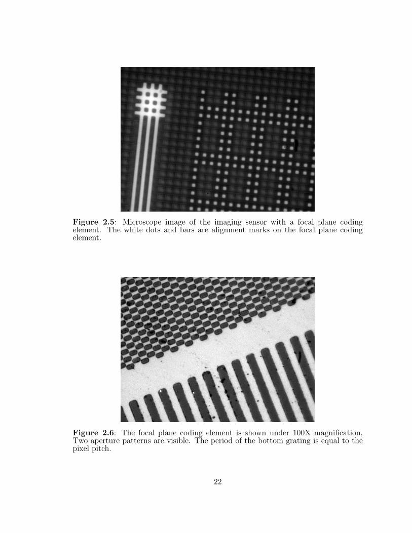
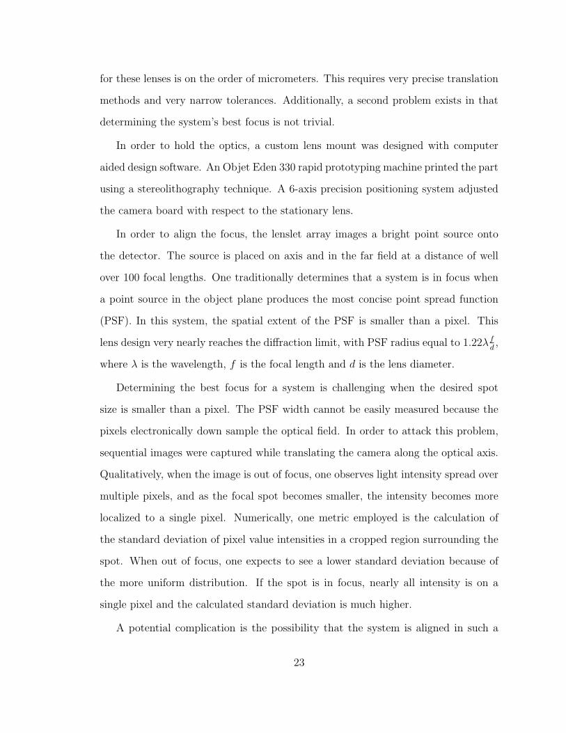
Figure 2.5: Microscope image of the imaging sensor with a focal plane codingelement. The white dots and bars are alignment marks on the focal plane codingelement.
Figure 2.6: The focal plane coding element is shown under 100X magnification.Two aperture patterns are visible. The period of the bottom grating is equal to thepixel pitch.
22
for these lenses is on the order of micrometers. This requires very precise translation
methods and very narrow tolerances. Additionally, a second problem exists in that
determining the system’s best focus is not trivial.
In order to hold the optics, a custom lens mount was designed with computer
aided design software. An Objet Eden 330 rapid prototyping machine printed the part
using a stereolithography technique. A 6-axis precision positioning system adjusted
the camera board with respect to the stationary lens.
In order to align the focus, the lenslet array images a bright point source onto
the detector. The source is placed on axis and in the far field at a distance of well
over 100 focal lengths. One traditionally determines that a system is in focus when
a point source in the object plane produces the most concise point spread function
(PSF). In this system, the spatial extent of the PSF is smaller than a pixel. This
lens design very nearly reaches the diffraction limit, with PSF radius equal to 1.22λfd,
where λ is the wavelength, f is the focal length and d is the lens diameter.
Determining the best focus for a system is challenging when the desired spot
size is smaller than a pixel. The PSF width cannot be easily measured because the
pixels electronically down sample the optical field. In order to attack this problem,
sequential images were captured while translating the camera along the optical axis.
Qualitatively, when the image is out of focus, one observes light intensity spread over
multiple pixels, and as the focal spot becomes smaller, the intensity becomes more
localized to a single pixel. Numerically, one metric employed is the calculation of
the standard deviation of pixel value intensities in a cropped region surrounding the
spot. When out of focus, one expects to see a lower standard deviation because of
the more uniform distribution. If the spot is in focus, nearly all intensity is on a
single pixel and the calculated standard deviation is much higher.
A potential complication is the possibility that the system is aligned in such a
23

way that, when in best focus, an impulse falls centered on the border between 2 (or
4) pixels. The resulting captured image would still show intensity split between those
pixels, even though the spot size is smaller than a single pixel.
However, the more interesting problem is determining the best focus for apertures
with a focal plane coding element. If a point source images to a masked region of the
detector, one would expect to see minimal response when the system is in best focus.
Furthermore, if the spot size grows, it could potentially increase the pixel response
of a given camera, with minimal effect on neighboring pixels. Thus, the result would
appear nearly identical to a situation where the system is in best focus imaging a
point source to an unmasked region on the detector. In order to differentiate between
the two, one needs to translate the image with respect to the camera pixels.
2.4 Impulse Response Measurement
The focal plane coding element modulates pixel responses differently in each aperture.
Since the period of the mask pattern is equal to the pixel spacing, pixels in a given
aperture all share identical modulation characteristics. However, determining the
exact registration of the mask with the camera pixels requires calibration.
A point source is approximated by a fiber coupled white light source placed in the
far field. When translating the focal plane array perpendicular to the optical axis, the
image of the point source moves correspondingly. Images were captured at multiple
point source locations. A computerized translation achieves subpixel positioning of
the point source on the detector. In Equation 2.1, f(x, y) ≈ δ(x, y) represents a
point source. Thus, we essentially measure the convolution of the lens’s PSF with
the sampling function of the detector.
First, consider the aperture with a binary grating with a 50% duty cycle. The
pattern is uniform in the horizontal direction. Facing the camera, this code appears
24

in the lenslet just below the open aperture. Figure 2.1 shows the designed focal
plane code on each pixel. For the scan, the center of the point source was translated
vertically in increments of 0.2 µm compared to the 5.2 µm pixel pitch. Figure 2.7
shows four adjacent pixels’ impulse responses as a point source is translated. Each
line plots the response of a pixel as a function of the relative movement of the point
source on the detector. The response gradually shifts from one pixel to the next as
the center of the point source tracks from one pixel to its neighbor. The width of
the impulse response measurement is broader than the 5.2µm pixel pitch because of
the finite extent of the PSF. Figure 2.8(a) shows the vertical impulse response scan
data for Aperture 5 whose code is shown in Figure 2.8. The open aperture’s impulse
response is modulated by the focal plane coding pattern into a two peaked response.
This same impulse response measurement was taken for a 2 dimensional array of
point source locations. Here, translation stages positioned a point source perpendic-
ular to the optical axis in a two dimensional grid as images are captured from the
camera. A typical scan might consist of 100x100 object locations covering approxi-
mately a 5x5 pixel square in image space.
Figure 2.9 shows impulse response data captured from an unmasked pixel. The
asymmetric nature of the CMOS pixel’s sampling is most likely a result of the pixel’s
lack of sensitivity where the charge to voltage circuitry resides. As expected, there
is only minimal variation between responses across apertures. This was verified by
observing nearly identical responses for pixels within a single subaperture. While
Figure 2.9 shows just a single pixel, data was collected for its neighbors and inspected
visually for consistency. The impulse response is shift invariant on a macro scale from
pixel to pixel, but shift variant within a single pixel.
Even more interesting, though, is the modulation of the impulse response shown
in Figures 2.10 and 2.11. The focal plane coding element’s effect is clearly visible.
25

0 5 10 15 20 250
50
100
150
200
250
300
Shift on Detector (µm)
Pix
el In
tens
ity
Figure 2.7: Impulse response scan of four adjacent pixels in the open aperture.Each line corresponds to a pixel’s intensity as a function of the relative position of apoint source on the detector plane.
26

0 5 10 15 20 250
20
40
60
80
100
Shift on Detector (µm)
Pix
el In
tens
ity
(a) Impulse response scan of four adjacent pixels in aperture 5. Each line corresponds to a pixel’sintensity as a function of the relative position of a point source on the detector plane.
−0.5 0 0.5
−0.5
0
0.5(b) Focal Plane Code for Aperture 5
Figure 2.8: Coded Impulse Response Scan for Aperture 5
27

Distance (µm)
Dis
tan
ce
(µ
m)
−10 −8 −6 −4 −2 0 2 4 6 8 10
−10
−8
−6
−4
−2
0
2
4
6
8
10
Figure 2.9: The 2D pixel impulse response as a function of image location ondetector plane.
The pixel exhibits a modified response due to the subpixel mask features. It is
important to note again that a precondition of this result is that the PSF of the
optical system is smaller than the features on the coding mask. Without such a
well confined spot, the mask would not have such a significant effect. A larger spot
would imply a narrower extent in the Fourier domain and would essentially low pass
filter the aperture sampling function. An impulse response shape similar to the open
aperture would be observed because the mask features (at higher spatial frequencies)
would be attenuated.
2.5 Single Image Construction
This section describes the computational construction of a single image from the
multiple images on the sensor subarrays. In addition to the conventional steps of
noise removal and deblurring, the reconstruction has the distinct decoding step for
integrating multiple images into a single image. This illustrates the reconstruction
procedure with the particular case of the modified Hadamard coding scheme.
28

Distance (µm)
Dis
tan
ce
(µ
m)
−10 −5 0 5 10
−10
−5
0
5
10
Distance (µm)
Dis
tan
ce
(µ
m)
−10 −5 0 5 10
−10
−5
0
5
10
Figure 2.10: Impulse response of a pixel masked with a 50% horizontal grating withperiod equal to the pixel pitch.
Distance (µm)
Dis
tan
ce
(µ
m)
−10 −5 0 5 10
−10
−5
0
5
10
Distance (µm)
Dis
tan
ce
(µ
m)
−10 −5 0 5 10
−10
−5
0
5
10
Figure 2.11: Impulse response of a pixel masked with a checkerboard with featuresize equal to one quarter pixel.
29

By the model (2.1), the subimage registered at each subaperture is considered as
a projection of the the same optical information along a different sampling channel.
The construction of a single image from the multiple projections is therefore a back
projection for image integration. The single-image construction consists of three
major stages. The first two stages prepare for the final back projection stage, or the
decoding stage.
First, every subimage corresponding to a lenslet is individually cropped from the
mosaic image captured at the sensor array. The subimage is registered according
to the sensor pixels associated with the lenslet. This cropping step requires the
calibration of the subarray partition and alignment. The calibration may be done
once for all in an ideal case, or carried out periodically or adaptively otherwise. Figure
2.12 shows the raw mosaic image, captured by the camera, of the ISO-12233 Digital
Still-Camera Resolution Chart.
Second, each and every subimage is processed individually for noise removal,
deconvolution of the corresponding lenslet distortions, as in the conventional image
processing. The additional task in this stage is the adjustment of the relative intensity
(in numerical values) between the subimages.
The final decoding stage follows Theorem 1. In terms of procedural steps, the
subimages are first integrated pixel block by pixel block. Specifically, for a P ×P lenslet array, the (i, j) pixel block is composed of the (i, j) pixels from P × P
subimages. Next, local to each and every pixel block, a block image of P×P subpixels
is constructed by using the explicit formula (2.10). Both steps are local to each pixel
block, or parallel among pixels blocks. This simple, deterministic and parallel process
has the great potential to be easily embedded into the imaging systems, using for
example Field Programmable Gate Array (FPGA) hardware. We omit the detailed
discussion on such embedding because it is beyond the scope of this paper.
30

Figure 2.12: A raw captured image from the multiple aperture focal plane codedcamera. Here, the target is a portion of an ISO-12233 Digital Still-Camera ResolutionChart.
31

(a) A detail of the multichannel reconstruc-tion.
(b) A bicubic spline interpolation of theclear aperture image.
Figure 2.13: Focal Plane Coded Camera Reconstruction Comparison
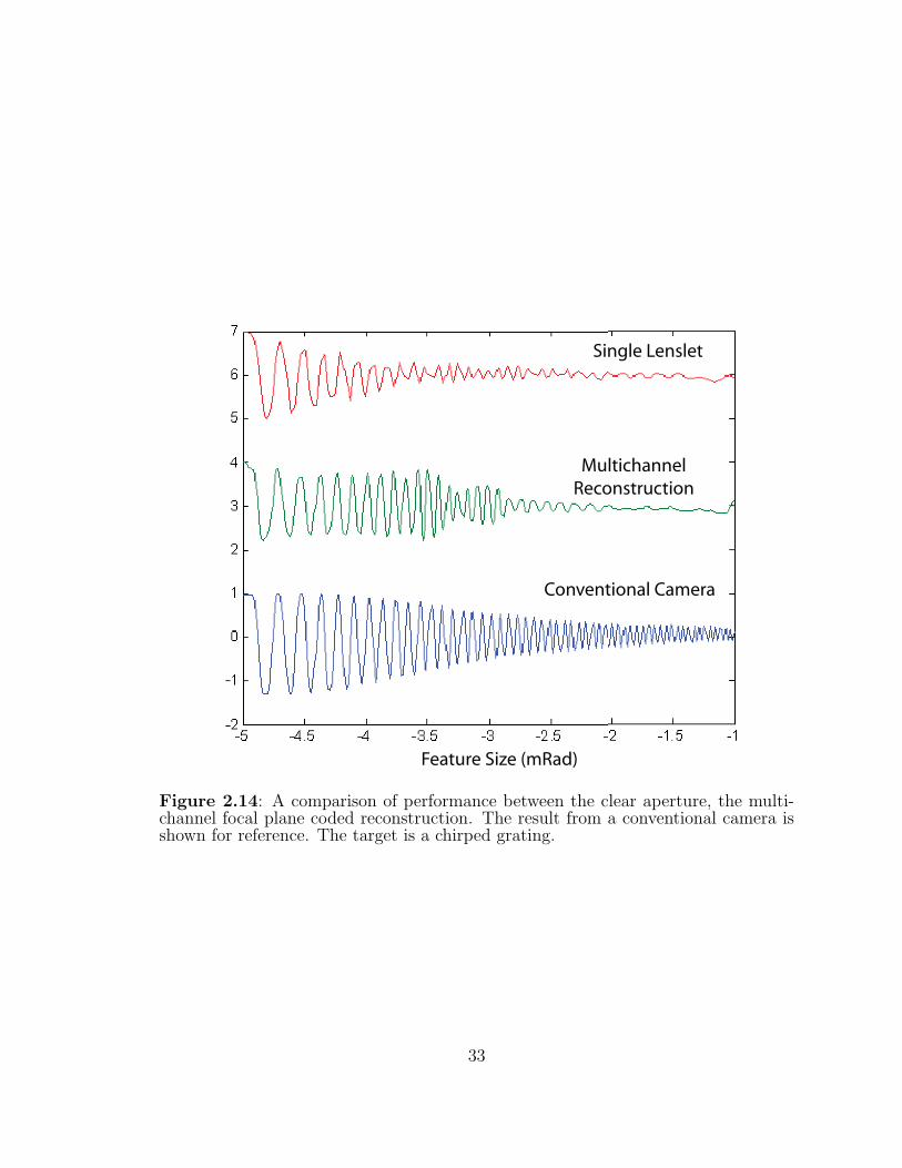
Figure 2.13 shows details of a reconstructed image (on the left) compared to the
bicubic spline interpolation of the clear aperture lenslet subimage (on the right). To
better visualize the reconstruction performance, a cross sectional pixel intensity plot
is shown in Figure 2.14. The target here is a chirped grating obtained by cropping a
section of an ISO-12233 Digital Still-Camera Resolution Chart.
2.6 Discussion
The success of a high-resolution optical imaging system equipped with a focal-plane
coding scheme relies on the integrated design and analysis of the coding and decoding
schemes with full respect to the potential and limitation of the physical implemen-
tation and numerical computation. This chapter presents a framework of focal-plane
coding schemes for multi-channel sampling in optical systems. Focal-plane coding
is a sampling strategy that modulates the intrinsic pixel response function. Among
other feasible schemes in the framework, we discussed lenslet displacements and cod-
ing masks. In the former scheme, the displacement pattern can be determined by
32
Single Lenslet
Multichannel
Reconstruction
Conventional Camera
Feature Size (mRad)
Figure 2.14: A comparison of performance between the clear aperture, the multi-channel focal plane coded reconstruction. The result from a conventional camera isshown for reference. The target is a chirped grating.
33

primary design and further calibration. The latter scheme has advantages in com-
putational efficiency and stability. While masks block photons, one could avoid this
loss by designing more complex sampling functions in the focal plane. Both coding
schemes in the COMP-I project were implemented.
Conventional systems image the scene onto the detector and sample that distri-
bution with a pixel array. These systems typically use the raw pixel intensity as the
estimate for the image in that location resulting in a sampling rate directly related to
pixel pitch. The COMP-I system does not use this sampling approach. By integrat-
ing the multichannel data we can achieve a smaller effective pixel size than what is
measured in the individual subimages. This system does not attempt to deconvolve
the optical PSF. Further, the best image recoverable from this technique is the one
that reaches the detector before any electronic sampling and after any optical blur.
The goal is to virtually subdivide raw electronic pixels by applying a different coding
pattern (or sampling function) to each lenslet (or channel). This is possible because
the coding mask has features on the scale of this virtual pixel size.
This chapter details a thin camera with lenslet array and focal plane coding
element to mask each lenslet differently. It also describes the physical system built
using custom optics and its alignment procedures. The system was tested to show
that the coding masks have the designed functionality.
34

Chapter 3
Multichannel Shift Coding
3.1 Introduction
This chapter describes thin cameras operating in the long-wave infrared (LWIR) band
(8-12 µm) using a 3× 3 lenslet array instead of a thicker single aperture optic. Each
of the nine individual sub-imaging systems are referred to as an aperture. The system
designed integrates optical encoding with multiple apertures and digital decoding.
The goal of this system is to use multiple shorter focal length lenses to reduce
camera thickness. Aperture size limits imaging quality in at least two aspects. The
aperture diameter translates to a maximum transmittable spatial bandwidth which
limits resolution. Also, the light collection efficiency, which affects sensitivity, is pro-
portional to the aperture area. A lenslet array regains the sensitivity of a conventional
system by combining data from all apertures. The lenslet array maintains a camera’s
etendue while decreasing effective focal length. However, the spectral bandwidth is
reduced.
The use of multiple apertures in imaging systems greatly extends design flexibility.
The superior optical performance of smaller aperture optics is the first advantage of
multiple aperture design. In an early study of lens scaling, Lohmann observed that
f/# tends to increase as f13 , where f is the focal length in mm [16]. Accordingly,
scaling a 5 cm f/1.0 optical design to a 30 cm focal length system would increase
the f/# to 1.8. Of course one could counter this degradation by increasing the
complexity of the optical system, but this would also increase system length and mass.
Based on Lohmann’s scaling analysis, one expects the best aberration performance
and thinnest optic using aperture sizes matching the diffraction limit for required
35

resolution. In conventional design, aperture sizes much greater than the diffraction
limited requirement are often used to increase light collection. In multiaperture
design, the light collection and resolution functions of a lens system may be decoupled.
A second advantage arises through the use of multiple apertures to implement gen-
eralized sampling strategies. In generalized sampling, a single continuously defined
signal can be reconstructed from independently sampled data from multiple non-
redundant channels of lower bandwidth. This advantage lies at the heart TOMBO-
related designs.
Third, multiple aperture imaging enables more flexible sampling strategies. Mul-
tiple apertures may sample diverse fields of view, color, time and polarization pro-
jections. There is a great degree of variety and flexibility in the geometry of multiple
aperture design, in terms of the relationships among the individual fields of views
and their perspectives to the observed scene. We focus in this paper, however, on
multiple aperture designs where every lens observes the same scene.
The COMP-I 1 Infrared Camera (CIRC ) uses digital super resolution to form an
integrated image. Electronic pixels often undersample the optical field. For LWIR in
particular, common pixel pitches exceed the size needed to sample at the diffraction
limited optical resolution. In CIRC the pixel pitch is 25 µm which is larger than the
diffraction limited Nyquist period of 0.5λf/#. This chapter shows that downsam-
pled images can be combined to recover higher resolution with a properly designed
sampling scheme and digital post processing.
In recent years, digital superresolution devices and reconstruction techniques have
been utilized for many kinds of imaging systems. In any situation, measurement
channels must be non-degenerate or non-redundant to recover high resolution infor-
mation. An overview of digital superresolution devices and reconstruction techniques
1COMP-I stands for the compressive optical MONTAGE photography initiative.
36

is provided by Park et al. [17]. While numerous superresolution approaches gather
images sequentially from a conventional still or video camera, the TOMBO system
by Tanida et al. [9] is distinctive in that multiple images are captured simultaneously
with multiple apertures. Another data driven approach by Shekarforoush et al. [18]
makes use of natural motion of the camera or scene. This chapter addresses digital
superresolution which should not be confused with optical superresolution methods,
such as structured illumination [19]. While digital superresolution can break the
aliasing limit, only optical superresolution can exceed the diffraction limit of an op-
tical system. The best possible resolution that can be obtained by CIRC cannot be
better than the diffraction limit of each of the nine subapertures.
CIRC was inspired by the TOMBO approach but differs in the design methodology
and in its spectral band. The diversity in multiple channel sampling with lenslets
is produced primarily by design with minor adjustment by calibration [20], instead
of relying solely on the inhomogeneity produced in fabricating the lenslets. CIRC
operates in the long-wave infrared band rather than the visible band. The DISP
group at Duke University has reported on the development and results of thin imaging
systems in the visible [21] range and the LWIR band [22], respectively.
This chapter describes a thin multiple aperture LWIR camera that improves on
previous work in a number of ways. It uses a more sensitive, larger focal plane ar-
ray, an optical design with better resolution and a modification in subsequent image
reconstruction. These changes give rise to significantly higher resolution reconstruc-
tions. Additionally this chapter provides a detailed noise analysis for these systems
by describing noise performance of the multichannel and conventional systems in the
spatial frequency domain.
The remainder of this chapter provides additional motivation for the use of mul-
tiple apertures in imaging systems. It outlines the main tradeoffs considered in our
37

system’s design and describe the experimental system. An algorithm to integrate
the measured subimages is presented, and sample reconstructions are included to
compare performance against a conventional system. Finally, numerical performance
metrics are investigated. Results of both the noise equivalent temperature difference
as well as the system’s spatial frequency response of each system are presented.
3.2 System Transfer Function and Noise
This section describes how the architectural difference between the multiaperture
camera and the traditional camera results in differences in modulation transfer, alias-
ing and multiplexing noise. This sections presents a system model and transfer func-
tion for multiaperture imaging systems. Noise arises from aliasing in systems where
the passband of the transfer function extends beyond the Nyquist frequency defined
by the detector sampling pitch. Multiaperture imaging systems may suffer less from
aliasing, however they are subject to multiplexing noise.
Digital superresoltuion requires diversity in each subimage. CIRC offsets the
optical axis of each lenslet with respect to the periodic pixel array. The lateral
lenslet spacing is not an integer number of pixels meaning the pixel sampling phase
is slightly different in each aperture. The detected measurement at the (n,m) pixel
location for subaperture k may be modeled as
gnmk =∫∞−∞
∫∞−∞
∫∞−∞
∫∞−∞ f(x, y)hk(x
′ − x, y′ − y)pk(x′ − n∆, y′ −m∆)dxdydx′dy′
=∫∞−∞
∫∞−∞ f(x, y)t(x− n∆, y −m∆)dxdy
(3.1)
where f(x, y) represents the object’s intensity distribution, hk(x, y) and pk(x, y) are
the optical point spread function (PSF) and the pixel sampling function for the kth
subaperture. ∆ is the pixel pitch. Shankar, et al. [22] discuss multiple aperture
38

imaging systems based on coding hk(x, y) as a function of k, and Chapter 2 discusses
systems based on coding pk(x, y). The focus here is on the simpler situation in which
the sampling function is independent of k and the difference between the images
captured by the subsapertures is described by a shift in the optical axis relative to
the pixel sampling grid, such that i.e. hk(x, y) = h(x − δxk, y − δyk). In this case,
Fourier analysis of the sampling function
t(x, y) =
∫ ∞
−∞
∫ ∞
−∞hk(x
′, y′)p(x− x′, y − y′)dx′dy′ (3.2)
yields the system transfer function (STF)
|t(u, v)| = |h(u, v)p(u, v)| (3.3)
Neglecting lens scaling and performance issues, the difference between the multi-
aperture and conventional single aperture design consists simply in the magnification
of the optical transfer function with scale. Fig. 3.1 compares the STFs of a conven-
tional single lens camera and a 3× 3 multichannel system. The plots correspond to
an f/1.0 imaging system with pixels that are 2.5 times larger than the wavelength,
e.g. 25 µm pixels and a wavelength of 10 µm. As in Equation 3.1, all apertures share
identical fields of view. For this plot, pixels are modeled as uniform sampling sensors,
and their corresponding pixel transfer function (PTF) has a Sinc based functional
form. The differing magnifications result in the conventional PTF being wider than
the multi-aperture case. Since the image space NA and the pixel size are the same
in both cases, the aliasing limit remains fixed.
The conventional system aliases at a frequency ualias = 1/(2∆). The aliasing limit
for multichannel system is determined by the shift parameters. If ∆xk = ∆yk = k∆/3,
then both systems achieve the same aliasing limit. The variation in sampling phases
39

0 0.05 0.1 0.15 0.2 0.25 0.30
0.2
0.4
0.6
0.8
1Conventional Camera
0 0.05 0.1 0.15 0.2 0.25 0.30
0.2
0.4
0.6
0.8
13 by 3 Multiple Aperture Camera
PTFOTFSTF
PTFOTFSTF
Figure 3.1: Comparison in system transfer functions between a conventional systemand a multiple aperture imager. The vertical line at 0.2 depict the aliasing limits foreach sampling strategy.
40

allows the multiple aperture system to match the aliasing limit of the single aperture
system. The difference between the two systems is that the pixel pitch and sampling
pixel size are equal to each other in a single aperture system, but the sampling pixel
size is effectively 3 times greater than the pixel pitch for the multiple aperture system.
Noise arises in the image estimated from gnmk from optical and electronic sources
and from aliasing. In this particular example, one may argue that undersampling of
the conventional system means that aliasing is likely to be a primary noise source.
A simple model accounting for both signal noise and aliasing based on Wiener filter
image estimation produces the means square error as a function of spatial frequency
given by
ε(u, v) =Sf (u, v)
1 + |STF (u, v)|2 Sf (u,v)
Sn(u,v)+|STF a(u,v)|2Sa(u,v)
(3.4)
where Sf (u, v) and Sn(u, v) are the signal and noise power spectra, and STFa(u, v)
and Sa(u, v) are the STF and signal spectrum for frequencies aliased into measured
frequency (u, v). As demonstrated experimentally in section 3.5, the multichannel
and baseline systems perform comparably for low spatial frequencies. Reconstruction
becomes more challenging for higher spatial frequencies as the STF falls off quicker in
the multichannel case (see Figure 3.1). If aliasing noise is not dominant, then there is
a tradeoff between form factor and noise when reconstructing high spatial frequency
components. Of course, nonlinear algorithms using image priors may substantially
improve over the Wiener MSE.
The ratio of the error for a multiple aperture and single aperture system as a
function of spatial frequency is plotted in Fig. 3.2. This plot assumes a uniform
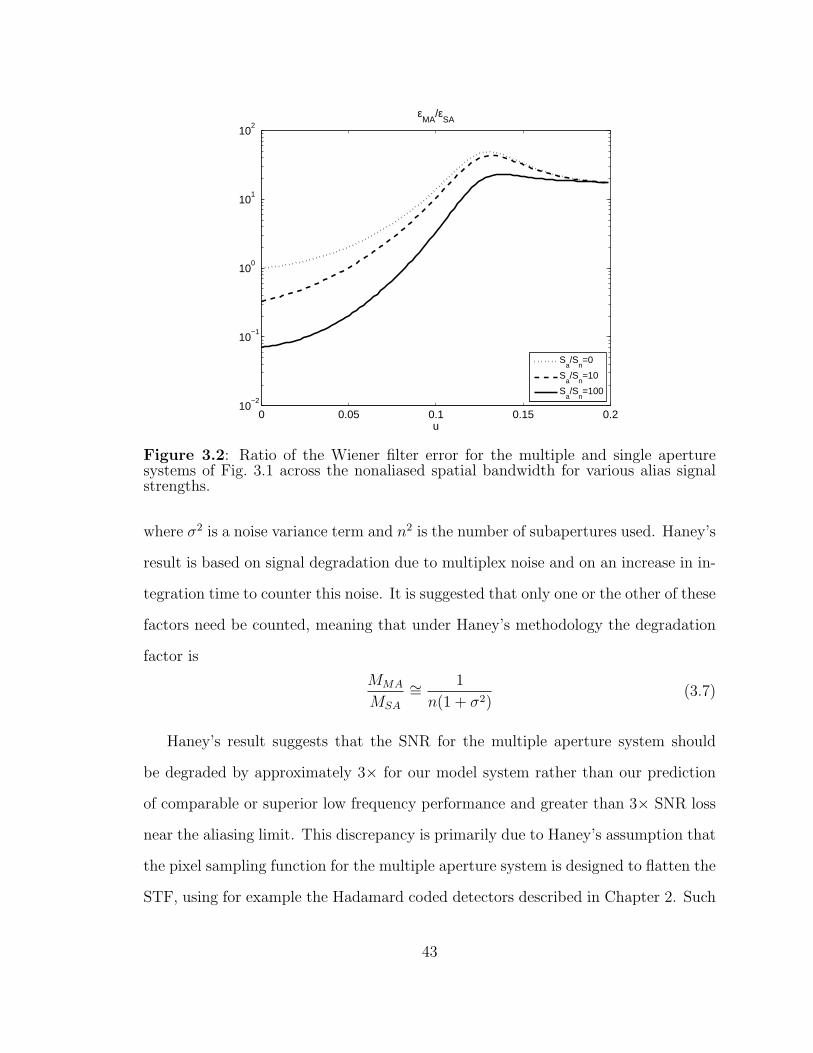
SNR of 100 across the spatial spectrum. The upper curve assumes that there is no
aliasing noise, in which case the STF over the nonaliased range determines the image
estimation fidelity. In this case, both systems achieve comparable error levels at low
41

frequencies but the error of the multiple aperture system is substantially higher near
the null in the MA STF and at higher frequencies. The middle curve assumes that
the signal level in the aliased band is 10% of the baseband signal. In this case, the
error for the multiple aperture system is somewhat better than the single aperture
case at low frequencies but is again worse at high frequencies. In the final example the
alias band signal level is comparable to the baseband. In this case, the lower transfer
function of the multiple aperture system in the aliased range yields substantially
better system performance at low frequencies relative to the single aperture case.
The point of this example is to illustrate that while the ideal sampling system
has a flat spectrum across the nonaliased band and null transfer in the aliased range,
this ideal is not obtainable in practice. Practical design must balance the desire to
push the spatial bandpass to the aliasing limit against the inevitable introduction of
aliasing noise. Multiple aperture design is a tool one can use to shape the effective
system transfer function. One can imagine improving on the current example by
using diverse aperture sizes or pixel sampling functions to reduce the impact of the
baseband null in the multiple aperture STF.
It is interesting to compare this noise analysis with an analysis of noise in multiple
aperture imaging systems developed by Haney [23]. Haney focuses on the merit
function
M =Ω
V Sδθ2(3.5)
where Ω is the field of view, δθ is the ifov, V is the system volume and S is the frame
integration time. Due to excess noise arising in image estimation from multiplex
measurements, Haney predicts that the ratio of the multiple aperture merit function
to the single aperture covering the same total area is
MMA
MSA
∼= 1
n3(1 + σ2)2(3.6)
42
0 0.05 0.1 0.15 0.210
−2
10−1
100
101
102
u
εMA
/εSA
Sa/S
n=0
Sa/S
n=10
Sa/S
n=100
Figure 3.2: Ratio of the Wiener filter error for the multiple and single aperturesystems of Fig. 3.1 across the nonaliased spatial bandwidth for various alias signalstrengths.
where σ2 is a noise variance term and n2 is the number of subapertures used. Haney’s
result is based on signal degradation due to multiplex noise and on an increase in in-
tegration time to counter this noise. It is suggested that only one or the other of these
factors need be counted, meaning that under Haney’s methodology the degradation
factor is
MMA
MSA
∼= 1
n(1 + σ2)(3.7)
Haney’s result suggests that the SNR for the multiple aperture system should
be degraded by approximately 3× for our model system rather than our prediction
of comparable or superior low frequency performance and greater than 3× SNR loss
near the aliasing limit. This discrepancy is primarily due to Haney’s assumption that
the pixel sampling function for the multiple aperture system is designed to flatten the
STF, using for example the Hadamard coded detectors described in Chapter 2. Such
43

coding strategies dramatically improve the high frequency response of the multiple
aperture system at the cost of dramatic reductions in low frequency image fidelity.
As illustrated in Fig. 3.1, simple shift codes provide poor high frequency response
but match the single aperture low frequency response.
Of course, the assumption underlying this discussion that MSE is a good image
metric can be challenged on many grounds. Numerous recent studies of feature spe-
cific and compressive sampling suggest that optimal sampling system design should
focus on robust sampling of image structure rather than pixel-wise sampling or STF
optimization. Rather than enter into a detailed discussion of the many denoising,
nonlocal or feature analysis and nonlinear signal estimation strategies that might be
considered here, we simply note that multiple aperture design appears to be a use-
ful tool in balancing constraints in focal plane design and read-out, optical system
design, system form factor and mass and imager performance.
3.3 Optical Design and Experimental System
Instead of a conventional lens, our system subdivides the aperture into a 3×3 lenslet
array. Each of these nine lenses meet the system’s required f-number, but achieves a
reduction in thickness by using shorter focal lengths. The position of each center of
the nine lenses has a unique registration with the underlying pixel array. This creates
measurement diversity which enables high resolution reconstruction. As was done by
Shankar et. al. [22], this design places each center with a 1/3 pixel shift with respect
to one another in two dimensions.
The underlying system goals motivated the design of the lenslet array: an ultra-
thin system with low f-number and excellent imaging performance over a broad field
of view. Each lenslet consists of a germanium meniscus lens and a silicon field flat-
tener. Both surfaces of the germanium lens are aspheric as is the top surface of the
44

silicon element. The bottom surface of the silicon element is planar. The f/1.2 lens
combination is 5 mm thick from the front surface of the lens to the detector package.
The full optical train is shown in Figure 3.3. Modulation transfer function (MTF)
plots of the designed system are shown in Figure 3.4.
Germanium
Cover WindowSilicon
Lens
Germanium
Lens
3.9 mm 1.03 mm
0.57 mm
Figure 3.3: The designed optical layout of a single lenslet.
The germanium element was diamond-turned on both surfaces, with the front and
back registered to each other within a few microns. Each lens was turned individu-
ally and mechanically positioned such that the decentration error is less than a few
microns. The silicon lens was made lithographically, using a gray scale High Energy
Beam Sensitive (HEBS) glass mask. The process exposes and develops a starting
shape in thick resist then uses reactive ion etching to transfer the shape into the
silicon. Sub-micron accuracy was achieved for the silicon element lenses.
The optics were attached to a 12-bit, 640 × 480 uncooled microbolometer array
with 25 µm square pixels. Each of the 9 lenslets images onto an area of about 80×80
pixels. This multiple aperture technique requires approximately one quarter of the
total detector pixels for image reconstruction. This uses such a large array primarily
because of its availability, but a commercial system would likely utilize a different
45
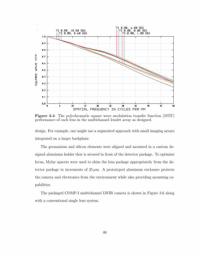
Figure 3.4: The polychromatic square wave modulation transfer function (MTF)performance of each lens in the multichannel lenslet array as designed.
design. For example, one might use a segmented approach with small imaging arrays
integrated on a larger backplane.
The germanium and silicon elements were aligned and mounted in a custom de-
signed aluminum holder that is secured in front of the detector package. To optimize
focus, Mylar spacers were used to shim the lens package appropriately from the de-
tector package in increments of 25 µm. A prototyped aluminum enclosure protects
the camera and electronics from the environment while also providing mounting ca-
pabilities.
The packaged COMP-I multichannel LWIR camera is shown in Figure 3.6 along
with a conventional single lens system.
46
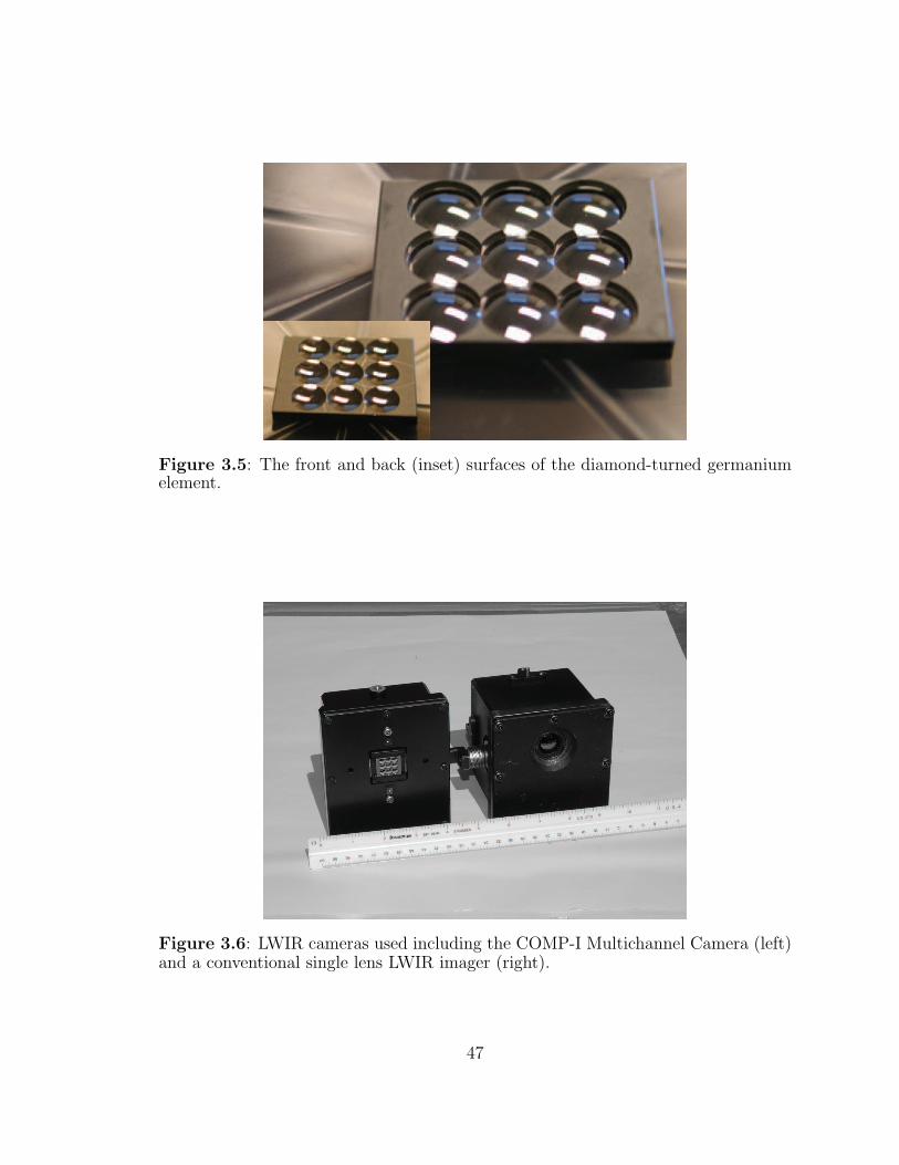
Figure 3.5: The front and back (inset) surfaces of the diamond-turned germaniumelement.
Figure 3.6: LWIR cameras used including the COMP-I Multichannel Camera (left)and a conventional single lens LWIR imager (right).
47

3.4 Image Reconstruction
There are nine lower-resolution images produced by the 3 × 3 lenslet array. The
reconstruction process consists of two stages, registration and integration.
3.4.1 Registration
It is critical to register sub-frames from the lower-resolution images. Due to paral-
lax, the relative image locations on the detector is dependent on object distance. To
register, one of the nine subimages is chosen as a reference. Then the two dimen-
sional correlation of that image with respect to the other eight cropped subimages is
maximized. This results in a coarse registration on the order of a pixel which greatly
improves efficiency of the reconstruction stage. These parameters may be saved as
calibration data because they are nominally constant for scenes of fixed depth. Coarse
registration data is applied in a second fine registration step described below.
3.4.2 Reconstruction
The downsampled images are integrated into a single one by the measurement equa-
tions,
Hk f = gk, k = 1, 2, . . . , 9
where f is the image of the scene at the resolution level targeted by the reconstruction,
gk is the image of lower resolution at the k-th sub-region of the detector array, Hk
is the discrete measurement operator related to the k-th aperture, mapping f to gk.
For the CIRC system, each measurement operator by design can be described in the
following more specific form
Hk = (D2,kB2,kS2,k)⊗ (D1,kB1,kS1,k), (3.8)
48

where Si, the displacement encoding at the aperture; Bi,k, i = 1, 2, describes optical
diffusion or blurring along dimension i associated with the k-th sub-aperture system;
and Di, the down sampling at the detector.
Iterative methods are used for the solution to the linear system, because the
number of equations is potentially as large as the total number of pixels on the
detector. Some algorithms that seem to work in simulation will fail to produce reliable
results with empirical data, primarily due to substantial discrepancy between ideal
assumptions and practical deviations. The reconstruction from measurements at the
early stage of a system development has to deal with insufficient calibration data on
system-specific functions and parameters as well as noise characteristics.
The underlying reconstruction model is called the Least Gradient (LG) model [24].
In the LG approach, the system of measurement equations is embedded in the fol-
lowing reconstruction model,
fLG = arg minf‖∇f‖2
s.t. Hk f = gk, k = 1, 2, . . . , 9(3.9)
where ∇ denotes the discrete gradient operator and ‖ · ‖2 is the Euclidean norm.
This LG model permits under-determined measurement systems. Among multiple
solutions, the LG solutions are smooth. In theory, the LG reconstruction model (3.9)
can be recast into the unconstrained minimization problem as follows,
fLG = arg mind∈N
‖∇(fp − d)‖2, (3.10)
where fp is a particular solution to the system of linear equations
Hkfp = gk, k = 1, 2, · · · , 9,
and N is the null space of the linear system. Denote by N a basis of the null space.
49

Then the solution to (3.10) can be expressed as follows:
fLG = fp −N(NT∇T∇N)−1(∇N)T∇fp.
Based on the separability of the measurement operator(s) as shown in (3.8) , we
apply the LG model to the subsystems partially and independently, i.e.,
fk,LG = arg minfk‖∇fk‖2
s.t. Hk fk = gk
(3.11)
for each and every k, 1 ≤ k ≤ 9. The solution to each of the individual partial
models can be obtained, using for example the explicit solution expression for the
corresponding unconstrained minimization problem.
This approach is similar to the Jacobi method for solving a large linear or non-
linear system of equations. While a sub-system is decoupled from the rest by parti-
tions in the measurements and the unknowns in the Jacobi method, a subsystem in
(3.11) is set by the natural partition in measurements gk, a separation in the objec-
tive function, an extension of the scalar-valued function f into the vector of partial
estimates [fk]k=1:9 and a substitution in the objective function. Simply stated, this
approach yields a stack of nine smooth images at the sub-pixel level in reference to
the detector pixels.
There is more than one way to integrate the stacked image estimates. There exist
multiple mappings from the vector-valued function to the scalar-valued function.
Technically, this mapping involves the alignment of the separate estimates fk, 1 ≤k ≤ 9, at the sub-pixel level. One shall notice that the relative displacements of the
lenslets do not play a significant role in the solution to each individual subsystem.
Practically, this sub-pixel alignment is carried out again by correlation, at the sub-
pixel level. The current registration method aligns the brightest regions in the field
50

of view to best maximize the correlation of the centers of the subimages. Misaligned
regions due to parallax are blurred as if out of focus. The separate image estimates in
alignment can then be integrated into one as a weighted sum, for example. When each
of the separated estimates is normalized in intensity, the weights are equal over well-
overlapped sub-pixels and unequal over non-overlapping sub-pixels. The estimate
by integration of the partial LG solutions can be used as the initial estimate for an
iterative method for the coupled system (3.9). Such initial estimates from empirical
data and without further refinement are shown in the next section.
Different algorithms may be used to upsample and integrate the data from each
channel. Figure 3.7 compare 3 different approaches. This image shows the reconstruc-
tion of a 4 bar target image. The top image uses the LG reconstruction algorithm
described above and shows the highest amount of contrast. The middle and bot-
tom images interpolate with a standard linear and bicubic algorithm respectively.
Each of the 9 channels are upsampled individually, and then the same alignment and
combination procedure as the LG approach is used to integrate the images.
The actual computation we perform for our current imaging system consists of
solving the subproblems Hk fk = gk for fk as above in (3.11), where Hk = (DB) ⊗(DB) with D = I ⊗ [111]/3 a linear operator that averages three contiguous pixels
down to a single pixel, B an approximate gaussian blurring operator common to all
lenslets and fk = (S2,k ⊗ S1,k)f . The shifts Sk are recovered with the correlation
alignment of the separate estimates fk.
In comparison to some other reconstruction algorithms, this approach via partial
LG solutions is computationally efficient and numerically insensitive to the boundary
conditions for the CIRC system.
51

5 10 15 20 25 30 35 40
20
40
60
80
100
120
Figure 3.7: Comparison of 3 different reconstruction approaches from the same rawdata. The top image uses the LG approach detailed in this paper and shows themost contrast. The middle and bottom image were formed using traditional linearand bicubic interpolation methods respectively.
3.4.3 Results
Results of the reconstruction algorithm demonstrate system performance. This sec-
tion includes data sets acquired at varying target ranges. Figure 3.8 shows the re-
construction of human subjects in a laboratory setting. Along with the processed
image this figure shows the raw data acquired directly off the camera. For compari-
son, a cubic spline interpolation upsamples a single lenslet image. Integration of the
multiple channels shows a clear improvement over this image.
To ensure the reconstructions do not introduce erroneous artifacts we compare
them to images taken with a conventional single lens LWIR camera. The comparison
system uses a 320×240 pixel array corresponding to approximately the same number
of imaging pixels used by the multichannel system. Both cameras share comparable
fields of view and utilize similar 25 µm microbolometer detector technology. For
the comparison system, internal electronics automatically adjust the gain level and
52
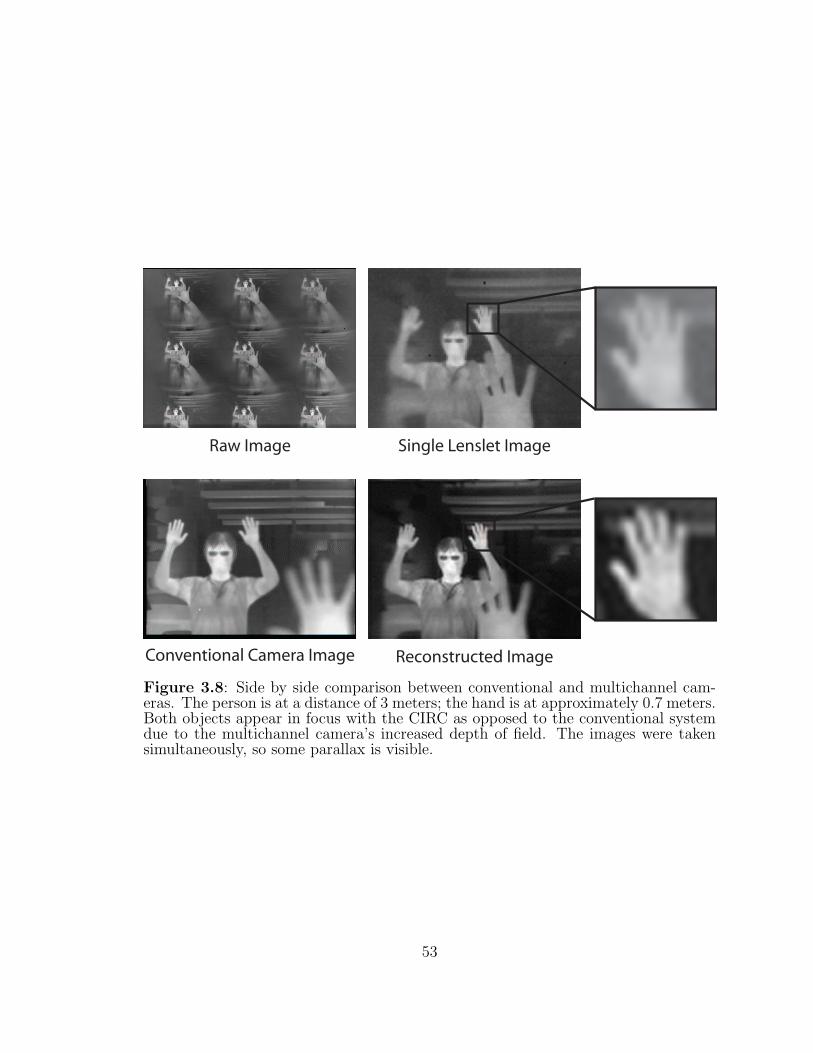
Raw Image Single Lenslet Image
Reconstructed ImageConventional Camera Image
Figure 3.8: Side by side comparison between conventional and multichannel cam-eras. The person is at a distance of 3 meters; the hand is at approximately 0.7 meters.Both objects appear in focus with the CIRC as opposed to the conventional systemdue to the multichannel camera’s increased depth of field. The images were takensimultaneously, so some parallax is visible.
53

output data through an analog RS-170 (black and white) video stream. A computer
capture card digitizes these video frames for analysis. The digitizer is the VCE-PRO
Flat PCMCIA card made by Imprex Incorporated. Unfortunately, direct digital
acquisition of pixel data was not possible for the comparison camera. The camera
was manually focused.
The images in Figure 3.8 also demonstrate the significantly larger depth of field
obtained by the multichannel system. The microlens array’s effective focal length of
6.15 mm is about 4 times shorter than the 25 mm focal length f/1.0 optic used in the
conventional camera. A shorter focal length translates to a much shorter hyperfocal
distance meaning close objects will appear more in focus.
Field data results show comparable performance between systems for targets at a
distance of 42 meters (i.e. long range). Figure 3.9 compares the multichannel results
to images from the conventional LWIR camera.
Conventional LWIR Camera Multichannel Reconstruction
Figure 3.9: Side by side comparison between conventional and multichannel cam-eras. Target distance is approximately 42m. Both cameras image with comparablequality.
54

3.5 Experimental Results
3.5.1 Noise Equivalent Temperature Difference
Thermal imaging systems are often calibrated to measure the equivalent blackbody
temperature distribution of a scene. In this application better performance means
better discrimination between two regions of different temperature. Noise Equivalent
Temperature Difference [25] is a metric for characterizing a system’s effective tem-
perature resolution. By definition, NETD is the temperature difference where the
signal to noise ratio is unity. NETD translates pixel fluctuations resulting from sys-
tem noise into an absolute temperature scale. As noise statistics vary with operating
temperature, the corresponding NETD fluctuates.
To experimentally calculate NETD, we image a collimated target aperture illumi-
nated with a blackbody source. The target projector optics consist of an all reflective
off-axis Newtonian telescope with a 2.75 degree field of view. The blackbody source
has a 52 mm clear aperture, and it illuminates a 37 mm diameter circular copper
target. Arbitrary target designs such as those shown in Figure 3.10 are milled in
small metal discs which are selected with a target wheel. The copper provides a
sufficient thermal mass to mask the blackbody source. Thus, the temperature of the
target and the background can be independently controlled. Figure 3.11 details the
experimental setup.
Effective NETD calculations are performed on large regions of constant temper-
ature to avoid a reduction in contrast by the camera’s optical system. Large targets
minimize high spatial frequency components. A full sized semicircle target (half
moon) is used for these measurements clearly segmenting two temperature regions.
To calculate NETD we use the following equation:
55

Figure 3.10: Copper targets used for collimator system.
Blackbody
Source
Target
Aperture
Primary
Mirror
Secondary
Mirror
Rotation
Stage
Multiaperture
Camera
Figure 3.11: Top-view of the experimental setup used for NETD and spatial fre-quency response measurements. A blackbody source illuminates a copper targetwhich is then collimated. The camera under test is positioned in front of the outputaperture of the projector.
56

NETD =∆T
SNR=
(TH − TB)mean(data|TH)−mean(data|TB)
std(data|TB)
(3.12)
TH and TB represent the ‘hot’ and ambient temperature regions created by a black-
body source and ∆T = TH−TB. The variables data|TH and data|TB represent arrays
of pixel values corresponding to those temperature regions. Here, signal is defined
as the difference between the mean pixel response in each area, and the noise is the
standard deviation of pixel values in the background region.
0 200 400 600 800 10000
2
4
6
8
10
Target Temperature Difference (mK)
SN
R
multichannelconventional
Figure 3.12: Signal-to-noise ratio (SNR) comparison as a function of target tem-perature difference. The circles and plus signs correspond to the conventional andmultichannel data points respectively.
Noise fluctuations influence NETD calculations, especially at low signal to noise
ratios. This is why NETD is traditionally calculated using higher contrast tempera-
ture regions. However, it may become problematic to do this using a computational
system because nonlinear processing will distort results using Equation 3.12.
The semicircle target was imaged at a number of different temperature contrast
settings and the results are shown in Figure 3.12. A linear regression is performed
57

on the data set to interpolate the temperature at which the SNR is unity. Using this
procedure, the NETDs for the conventional and multichannel cameras are 121 mK
and 131 mK, respectively. Since both cameras utilize similar uncooled focal plane
technology these fairly comparable results are expected. This discrepancy is likely
due to the different lens transmissions of the two systems. Their total area, number
of elements, and anti-reflective coatings are not identical.
3.5.2 Spatial Frequency Response
This subsection outlines an alternate interpolation method to combine our multi-
channel data. Aliasing is removed to recover contrast from bar targets with spatial
frequencies beyond the Nyquist limit defined by the pixel pitch. High resolution
results are recovered by combining discrete samples from each subaperture with reg-
istration information. Characterization of the subpixel shift of each channel gives
the crucial reference needed for these reconstructions. Using a collection of peri-
odic targets, it is possible to experimentally measure the systems spatial frequency
response.
The Whittaker-Shannon interpolation formula gives the following expansion to
reconstruct a continuous signal from discrete samples:
f(x) =∞∑
n=−∞f(
n
2B)sinc(2Bx− n) (3.13)
The reconstructed bandwidth, B, is related to the sampling interval ∆ as: ∆ =
1/2B. This strategy of recovering a continuous signal from discrete samples provides
the basis for combining our multichannel data.
For the 3 × 3 system presented in section 3.3, the lenses are positioned with
1/3 pixel offsets in 2 dimensions and all share the same field of view. Thus, in the
58

absence of parallax, the individual subimage data could be interweaved on a grid
with a sampling period equal to one third the nominal pixel size.
Generalizing Equation 3.13 to allow for multiple channels we obtain:
f(x) =K∑
k=1
N/2∑
n=−N/2
mk[n]sinc(2B′x− n + δk) (3.14)
Here, mk represents the discrete samples measured from channel k. The offset
registration between each of these sampling train is accounted by the δk parameter.
Nominally, δk = k∆K
. Also recognize that B′ can be increased to KB because an
increased sampling rate extends system bandwidth. Any choice of B′ < KB is
equivalent to simply low pass filtering the reconstructed signal. With a 33% fill
factor, one could directly interleave the multichannel data without the need for this
sinc interpolation strategy. However, a higher fill factor does not directly imply
limited resolution. The pixel’s sampling function acts as a spatial filter which limits
reconstruction contrast in the presence of noise.
This system only approximates the designed 1/3 pixel lenslet shifts. What follows
is the characterization procedure used to register the channels and arrive at slightly
modified δk parameters. Reconstruction on nonideally sampled data is a growing
research area studied by Unser [26] and others [27,28]. This reconstruction approach
would not be appropriate for significant misalignments. However, better reconstruc-
tion results are achieved by tuning the registration parameters to the physical system.
First, the camera is mounted on a motorized rotation stage in front of the target
projector discussed in Section 3.5.1. An appropriate temperature setting is chosen
for good contrast. The stage rotates the camera in regular controlled steps shifting
the target on the detector a fraction of a pixel at each step. Simultaneously from
each aperture we record data at every camera position. The full scan should result
59

in the target moving by a handful of pixels on the detector. This set of registered
frames from each channel contains registration information.
To create diversity in each aperture, the lenslet pitch was designed to be a non-
integer multiple of the pixel width. Each channel measures the same object, but it is
recorded with a unique offset. More specifically the attempt is to prescribe a unique
1/3 pixel stagger in x and y for each of the 9 lenslets. Through correlation or other
strategies, shift information can be extracted from the position information. Figure
3.13 plots the responses from a pixel in each of 3 channels to a periodic bar target
as a function of camera angle. The position based offset between signals is directly
related to the subpixel registration of each channel.
−0.5 0 0.50
100
200
300
400
500
600
700
800
Angular Position (degrees)
Inte
nsity
(ar
b. u
nits
)
Normalized Pixel Responses
Lenslet 1Lenslet 2Lenslet 3
Figure 3.13: Registered responses of a pixel in each aperture for a rotating targetscene.
Interpolations are provided to demonstrate the recovery of higher resolution data
from registered downsampled multichannel data. In the extreme cases, each down-
sampled channel samples below it’s corresponding “Nyquist” limit measuring aliased
data. Reconstruction is contingent upon two major factors. First, the high perfor-
60

mance optical system must maintain the higher spatial frequencies (or resolution)
when imaging onto the pixel array. Second, the subpixel shifts between each channel
mk must be adequately characterized.
The data from Equation 3.14 and the characterization information from Figure
3.13 is used to generate a resolution improvement in one dimension by processing
data from three apertures on a row by row basis. Figure 3.14 shows a side by
side comparison between the raw data and interpolation for a vertically placed 4
bar target. The bar width in the target aperture is 3.18 mm. Using the collimator
focal length of 762 mm, the calculated spatial frequency is 0.120 cycles/mrad. High
contrast levels are present in the subapertures as well as the reconstruction. This same
approach is also used on a more aggressive target. The raw data and interpolation
for a target with 1.98 mm features (0.192 cy/mrad) are shown in Figure 3.16. This
target corresponds to a period of 32.2 µm on the focal plane. As this is smaller
than twice the 25 µm pixel pitch, recovery of contrast demonstrates superresolution
reconstruction. Figure 3.17 shows an intensity plot for one row. The 4 peaks in the
interpolation (solid line) correspond to the 4 bars of the target. Using one subaperture
alone (circles), it would be impossible to resolve these features. Further, the left 2
bars in the conventional systems response (dotted line) are nearly indistinguishable.
For these reconstructions B′ = 1.7B, which is slightly less than the theoretical
factor of 3 improvement possible with this system. Misalignment fundamentally lim-
its the full capability. As mentioned above, this conservative interpolation result is
equivalent to low pass filtering. However, this choice of B′ > B allows for demon-
stration of the alias removal capabilities of the process. Note that these results are
generated from a single row vector from 3 apertures. While the approach is extend-
able to two dimensions, some experimental difficulties limit our abilities to provide
them here. Subpixel alignment and registration challenges and nonuniformity are the
61
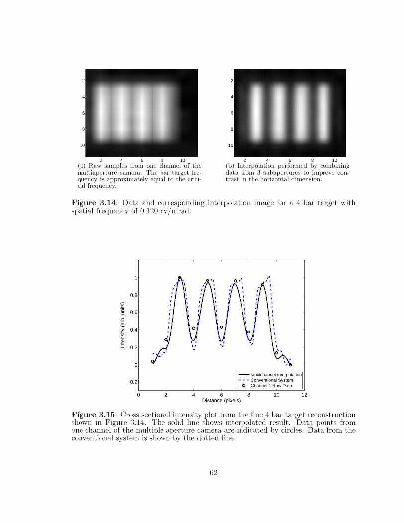
2 4 6 8 10
2
4
6
8
10
(a) Raw samples from one channel of themultiaperture camera. The bar target fre-quency is approximately equal to the criti-cal frequency.
2 4 6 8 10
2
4
6
8
10
(b) Interpolation performed by combiningdata from 3 subapertures to improve con-trast in the horizontal dimension.
Figure 3.14: Data and corresponding interpolation image for a 4 bar target withspatial frequency of 0.120 cy/mrad.
0 2 4 6 8 10 12
−0.2
0
0.2
0.4
0.6
0.8
1
Distance (pixels)
Inte
nsity
(ar
b. u
nits
)
Multichannel InterpolationConventional SystemChannel 1 Raw Data
Figure 3.15: Cross sectional intensity plot from the fine 4 bar target reconstructionshown in Figure 3.14. The solid line shows interpolated result. Data points fromone channel of the multiple aperture camera are indicated by circles. Data from theconventional system is shown by the dotted line.
62

2 4 6 8 10
2
4
6
8
10
(a) Raw samples from one channel of themultiaperture camera. Aliased data is mea-sured because the bar target frequency ex-ceeds the critical frequency.
2 4 6 8 10
2
4
6
8
10
(b) 3 channel interpolation demonstratingresolution improvement in the horizontal di-mension.
Figure 3.16: Data and corresponding interpolation image for a 4 bar target withspatial frequency of 0.192 cy/mrad.
0 2 4 6 8 10 12
−0.2
0
0.2
0.4
0.6
0.8
1
Distance (pixels)
Inte
nsity
(ar
b. u
nits
)
Multichannel InterpolationConventional SystemChannel 1 Raw Data
Figure 3.17: Cross sectional intensity plot from the fine 4 bar target reconstructionshown in Figure 3.16. The solid line shows interpolated result. Data points from onechannel are indicated by circles. Data from the conventional system (dotted line)show that the target frequency approaches the aliasing limit.
63

major limiting factors.
This work demonstrates the recovery of contrast from aliased data samples. To
quantify the results, fringe visibilities are calculated for multiple 4 bar targets with
each one corresponding to a different spatial frequency. The following formula is used
to quantify the contrast:
V =Imax − Imin
Imax + Imin
(3.15)
where Imax and Imin represent the average of intensities of the 4 local maxima and 3
local minima, respectively. Table 3.1 compares these calculated values to the response
of a single lenslet in the multichannel system as well as a conventional imaging system.
Table 3.1: Experimentally calculated contrast, V , for 4 bar targets at 5 spatialfrequencies.
Calculated Target Conventional Single MultichannelSpatial Frequency System Lenslet Reconstruction
(cy/mrad) Contrast Contrast Contrast0.120 77% 40% 60%0.136 55% 20% 28%0.150 55% aliased 18%0.167 40% aliased 14%0.192 31% aliased 11%
3.6 Conclusion
This chapter extends the field of multiple aperture imaging by describing the design
and implementation of a thin LWIR camera using a 3× 3 lenslet array. The multiple
aperture approach provides a thickness and volume reduction in comparison to a
conventional single lens approach. To form a single image, the 9 subimages are
combined computationally in post processing.
A working prototype has been constructed, and its data has been extensively
64

analyzed. A LG image reconstruction algorithm has been implemented that shows
better results than linear and spline interpolation. The quality of natural scene im-
agery appears comparable to that produced by a conventional single lens camera.
Quantitatively, similar Noise Equivalent Temperature Difference results are obtained
between these two systems. Reconstruction requires system characterization that in-
volved determining the relative subpixel registration of each lenslet by scanning a high
frequency target with subpixel precision. Bar target data at multiple spatial frequen-
cies was reconstructed using these registration parameters. This chapter shows the
combination of aliased data from multiple subapertures to reconstruct high frequency
bar targets. Joint post processing of the subimages improves resolution beyond the
limit of a single lenslet.
65

Chapter 4
Multichannel Narrow Band Spatiospectral
Coding
4.1 Introduction
Spectral imaging results in a one dimensional spectrum vector at every point in a
two dimensional image, thus forming a three dimensional “datacube”. The spatial
and spectral content of a scene can be analyzed to perform object identification and
recognition, and wide-area chemical analysis. There are numerous applications in the
fields of environmental sensing, military targeting and tracking, medical diagnostics,
and industrial process control.
xy
λ
Figure 4.1: DatacubeA graphical representation of the datacube depicting 2 dimensions of spatial
information and 1 dimension of spectral information
Traditional color digital cameras are essentially three channel (red, green, and
blue) broadband spectral cameras. Consumer focal planes commonly accomplish
this differentiation by incorporating a mosaic of color filters directly on the pixels.
66

Bayer of Eastman Kodak was the first to introduce this technique [29]. Figure 4.2
depicts a common arrangement utilizing 50% green, 25% red, and 25% blue, and
alternate patterns exist.
Figure 4.2: Bayer PatternThe Bayer arrangement of color filters on the pixel array of an image sensor.
(source: http://en.wikipedia.org/wiki/File Bayer pattern on sensor.svg)
This paradigm is widespread for visible color imaging, and the strategy is com-
pelling for mass production. Interference filters are not common on cameras sensitive
in other wavelength bands due to limited demand and increased design complexity.
In addition, specific applications require different spectral ranges and resolutions. In
these situation custom thin film color filters would likely not be practical.
This chapter presents a novel technique to perform multichannel narrow band
spectral imaging. It uses a collection of optical elements to spectrally filter a scene
differently at each pixel location. Similar color mosaic data is obtained, but the
generation is different.
The sampling of narrow band spectral channels represents one major departure
from conventional color imaging. Narrow band sampling becomes much more complex
if it were implemented using traditional pixel filtering methods such as organic dye
67

or dielectric stacks. Sharper spectral responses require more dielectric layers than
required for broadband designs.
This method provides a much more inexpensive and robust way to perform spec-
tral imaging than other approaches. It makes it much more feasible to operate in
non-visible wavelength bands since it requires only lenses, prisms, and aperture masks
in combination with a broadband focal plane array. A prototype system in the long
wave infrared is constructed to demonstrate four channel spectral imaging in this
challenging light band. This is a relatively low cost system in comparison to a two
band spectral imaging with thin-film interference filters by Gluck et. al. [30] which
requires a custom focal plane array.
Spectral imaging in the LWIR opens the possibilities to extract much more infor-
mation about a scene. Traditional LWIR cameras only measure the relative intensity
at each pixel location. A false color may be applied to the images by coloring re-
gions radiating more power as hot. These methods assume that all objects share the
same emissivity; they do not necessarily reflect an object’s absolute temperature or
spectrum. A blackbody radiator’s temperature defines the spectrum of light emit-
ted, however, the total power radiated is also a function of emissivity. Multispectral
imaging enables joint estimation of an object’s temperature and emissivity. Further-
more, it enables differentiation of traditional blackbody sources from those with more
complex radiation or reflective spectra.
4.2 Elementary Example
Spectral imaging relies on building optical systems that provide the ability to create
an impulse response that varies in wavelength. This is achieved by manipulating the
datacube. Fortunately, tools are available to manipulate the datacube with known
transformations. Three fundamental transformation are:
68
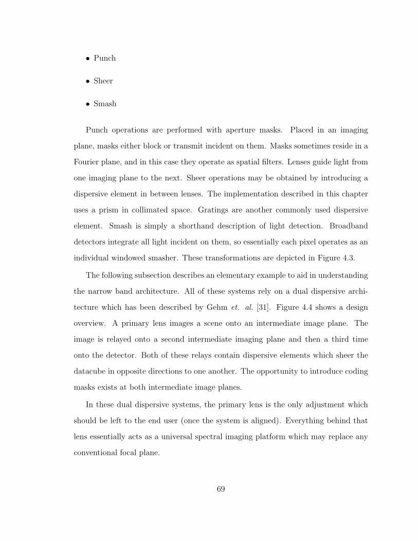
• Punch
• Sheer
• Smash
Punch operations are performed with aperture masks. Placed in an imaging
plane, masks either block or transmit incident on them. Masks sometimes reside in a
Fourier plane, and in this case they operate as spatial filters. Lenses guide light from
one imaging plane to the next. Sheer operations may be obtained by introducing a
dispersive element in between lenses. The implementation described in this chapter
uses a prism in collimated space. Gratings are another commonly used dispersive
element. Smash is simply a shorthand description of light detection. Broadband
detectors integrate all light incident on them, so essentially each pixel operates as an
individual windowed smasher. These transformations are depicted in Figure 4.3.
The following subsection describes an elementary example to aid in understanding
the narrow band architecture. All of these systems rely on a dual dispersive archi-
tecture which has been described by Gehm et. al. [31]. Figure 4.4 shows a design
overview. A primary lens images a scene onto an intermediate image plane. The
image is relayed onto a second intermediate imaging plane and then a third time
onto the detector. Both of these relays contain dispersive elements which sheer the
datacube in opposite directions to one another. The opportunity to introduce coding
masks exists at both intermediate image planes.
In these dual dispersive systems, the primary lens is the only adjustment which
should be left to the end user (once the system is aligned). Everything behind that
lens essentially acts as a universal spectral imaging platform which may replace any
conventional focal plane.
69

xy
λ
(a) Punchx
y
λ
(b) Sheer
xy
λ
(c) Smash
Figure 4.3: 3 fundamental datacube transformations.
Dispersion Optics
(in collimated space)
Collimating
Lens
Detector
Plane
Intermediate
Image Plane
Coding Mask
Collimating
Lens
Imaging
Lens
Object Space
Intermediate
Image Plane
Coding Mask
Collimating
Lens
Collimating
Lens
Dispersion Optics
(in collimated space)
P2M2M1 P1L1 L2 L3 L4 L5
Figure 4.4: Dual-disperser hyperspectral imaging architecture.
70

4.2.1 Direct measurement of individual wavelength channels
The implementation of the example can be achieved with two equal and opposite
dispersive elements and one coding mask. This is a non-multiplexed simplification
of the system proposed by Gehm et. al. [31]. The system produces a color filtered
image on the detector. Analogous to the Bayer pattern, each detector pixel measures
only one color band. However, the filtering here is achieved through dispersive optics
and a modulating mask aperture instead of wavelength filters on each pixel.
It may be helpful to imagine the system’s performance if the coding mask was
removed. In this situation, the dispersive stages cancel each other, and an image of
the first intermediate image plane is relayed onto the detector. The detector pixels
integrate a conventional broadband image.
Introducing the mask punches holes through a sheered datacube which imposes
a spatially varying spectral filter on the scene. And the mask is designed to block
all but one spectral channel per object location. Since the center wavelength of this
bandpass filter varies spatially, a different channel is passed based depending on the
pixel’s spatial location.
In more detail, a scene is imaged onto a coding mask through dispersive optics.
This dispersion introduces a lateral shift in the scene based on wavelength. Along
this dispersive direction, the coding mask contains regularly spaced openings with
period equal to the dispersion distance for the full system bandwidth on the coding
mask. There is only one opening per period, and the duty cycle of the mask is equal
to the reciprocal of the number of channels. A second stage relays the image of the
mask onto the pixel array. This set of optics removes all the dispersion introduced
by the first set of optics so that the resulting image on the detector is registered.
Since the mask selectively transmits only one wavelength channel at each pixel, the
resulting measured image is essentially a color filtered image.
71

Intermediate
Image Plane
Intermediate
Image Plane
(with mask)
Pixel Array
The full bandwidth of light incident
on an element is dispersed on the
intermediate image plane.
Periodic slits on the mask
selectively transmit only one
wavelength channel for each
location.
A second set of optics relays the
light onto the detector, removing
the dispersion introduced.
The linewidth of each
channel is approximately
the total system bandwidth
divided by the number of
channels.
Light originating from adjacent
locations on the intermediate image
plane overlaps on the mask, but there
is no ambiguity on the detector.
A scene is imaged onto
the intermediate
image plane by an
objective lens.
Every detector
pixel corresponds
to a registered
location on the
intermediate
image plane.
Figure 4.5: A one dimensional (cross section) diagram detailing the direct measure-ment of individual spectral channels. This graphic superimposes the light path from3 object locations. White light illuminates each pixel. The overlap shows how redlight from one object location and blue light from another map to the same locationon the coding mask.
72

4.3 System Architecture
The overall goal of the prototype system built is to measure four narrow band channels
of LWIR light centered at 8.25, 9.2, 10, and 10.75 µm. This section describes the
overall architecture and section 4.5 specifies the design parameters in more detail.
The introduction of more than one patterned aperture mask in spectral imagers
offers greater flexibility to design more complex spectral sampling functions. This
design includes two coded apertures to selectively measure narrow spectral bands at
periodic spatial locations in 2 dimensions. However, the technique extends to the use
of 2 or more cascaded stages of dispersive optics and coding masks.
The effective system here maps all spectral channels of interest from a spatial
location to adjacent pixel locations on the detector. This group of pixels corresponds
to a single object ’pixel’ whose full spectrum is measured in a single time step. Each
detector pixel measures exactly one spectral channel in a single object location. The
spectral channels are not coupled or multiplexed on the detector in this implementa-
tion. Since the spectral channels from a given object location are split across multiple
pixels and measured individually, not every spatial location can be measured. The
spatial sampling structure of this system is periodic. Additionally, the system can be
designed to accommodate a full range of fields of view.
There are two intermediate image planes in this system in addition to the image
plane at the detector. A coded aperture mask is introduced at each intermediate
image plane, modulating the intensity transmittance. An objective lens images the
scene of interest onto the first mask. The aperture code selectively transmits certain
object locations and blocks other points in the object. This mask acts solely as a
spatial filter. The next stage of the system images this plane through a dispersive
element onto a second intermediate image plane. This dispersion introduces a lateral
shift in the object based on wavelength. Thus only the spectra from certain object
73
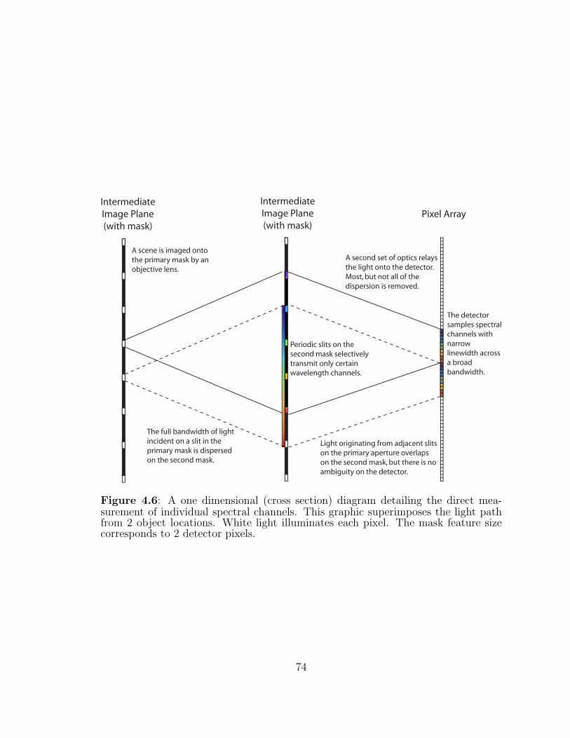
Pixel Array
The full bandwidth of light
incident on a slit in the
primary mask is dispersed
on the second mask.
Periodic slits on the
second mask selectively
transmit only certain
wavelength channels.
A second set of optics relays
the light onto the detector.
Most, but not all of the
dispersion is removed.
The detector
samples spectral
channels with
narrow
linewidth across
a broad
bandwidth.
Light originating from adjacent slits
on the primary aperture overlaps
on the second mask, but there is no
ambiguity on the detector.
A scene is imaged onto
the primary mask by an
objective lens.
Intermediate
Image Plane
(with mask)
Intermediate
Image Plane
(with mask)
Figure 4.6: A one dimensional (cross section) diagram detailing the direct mea-surement of individual spectral channels. This graphic superimposes the light pathfrom 2 object locations. White light illuminates each pixel. The mask feature sizecorresponds to 2 detector pixels.
74

locations get dispersed onto the second intermediate image plane.
At the second intermediate image plane, a mask spatially modulates the light.
However, because of the dispersion introduced, the second mask acts as a spatiospec-
tral filter on the original source datacube. For the design disclosed, the second mask’s
transmittance is identical to the first mask. The periodic structure of this element
essentially combs the dispersed spectra and is responsible for creating very sharp
linewidths associated with each channel. The exact designs of the masks are func-
tions of the desired spectral response.
The implemented design introduces a relatively larger amount of dispersion in
comparison to the system designed in Section 4.2.1. Because of this, an equivalent
sized opening on the secondary mask introduces a very sharp spectral response. The
last set of relay optics images the transmitted light from the second intermediate
image plane onto the detector plane. In this design, the dispersive optics remove
most, but not all of the dispersion. The wavelength channels do not all return to
a single pixel, rather they map to a linear group of pixels. This makes it possible
to directly measure each wavelength channel individually. With the disclosed design
there is no ambiguity on the detector because the dispersive amounts are chosen in
conjunction with the period of the first coded aperture to ensure channels from one
spatial location do not overlap their neighbor.
4.4 Mathematical Model
This transfer function analysis models the intensity of each spectral channel at each
image plane. The masks, dispersive elements, and optics are all considered ideal for
this basic analysis.
The primary lens of this system focuses the source onto the first mask aperture.
The object distribution is modeled as a 3 dimensional function S(x, y; λ). Since
75

masks solely act as spatial filters, they modulate all spectral channels at a given
spatial location equally. The intensity distribution immediately after transmission
through the first mask can be described as
S0(x, y; λ) = S(x, y; λ)T1(x, y) (4.1)
where T1(x, y) is the transmittance of the first mask.
The spectral density just prior to the second intermediate image plane is given by
S1(x, y; λ) =
∫ ∫dx′dy′δ(x′ − [x + α(λ− λc)])δ(y
′ − y)So(x′, y′; λ)
= S(x + α(λ− λc), y; λ)T1(x + α(λ− λc), y)
(4.2)
Here the Dirac delta functions describe propagation through unity-magnification
imaging optics and a dispersive element with linear dispersion α and center wave-
length λc. Note this model assumes linear dispersion, which is approximately true
only over limited wavelength ranges.
In general, letting T2(x, y) represent the transmittance of the second mask, the
spectral density just after the second intermediate image plane is
S2(x, y; λ) = S1(x, y; λ)T2(x, y)
= S(x + α(λ− λc), y; λ)T1(x + α(λ− λc), y)T2(x, y)(4.3)
Finally, a second set of optics relay the image through another dispersive element
with a different linear dispersion β and equal center wavelength λc. The spectral
76

density at the detector, S3(x, y; λ) is given by
S3(x, y; λ) =
∫ ∫dx′dy′δ(x′ − [x + β(λ− λc)])δ(y
′ − y)S2(x′, y′; λ)
= S2(x− β(λ− λc), y; λ)
= S(x + (α− β)(λ− λc), y; λ)
× T1(x + (α− β)(λ− λc), y)T2(x− β(λ− λc), y)
(4.4)
4.5 System Implementation and Components
The following section describes the components used to implement the multichannel
narrow band spectral camera. Figure 4.7 shows the fully integrated system.
Figure 4.7: A photograph of the fully integrated LWIR mutlispectral system.
4.5.1 Camera and Lenses
The system is built on a 640 × 480 uncooled microbolometer array manufactured
by Raytheon Company. This focal plane array has 25 µm square pixels. Since dig-
ital output of this camera was unavailable, a VCE-PRO Flat PCMCIA card made
77

by Imprex Incorporated digitized the analog video output. A software interface to
the camera allows for tuning of the gain and offset parameters as well as resetting
the nonuniformity correction (NUC). Variations in the pixel to pixel response are
minimized through the use of NUC.
4.5.2 Mask Design
Two identical masks are used in this system. The duty cycle of the periodic square
wave pattern (in the dispersion direction) is 25% which reflects the desire to measure
4 spectral bands. This system uses horizontal dispersion, so all the rows operate
independently. One mask implementation could be a series of vertical slits. However,
the masks chosen for this system staggered the mask features, and Figure 4.8 shows
the pattern. The stagger creates a more uniform spatial sampling pattern.
The use of 2 × 2 pixels per mask feature reduces the MTF requirements on the
lenses and reduces the cross-talk between the spectral channels. This leads to 50 µm
features given the 25 µm pixel pitch.
50 μm
50 μm
Figure 4.8: Cropped region of designed mask aperture showing repeated patternwith 50 µm feature size.
78

4.5.3 Prism Design
Two sets of two-element prisms provide the dispersion. A two-element design keeps
the system coaxial, reduces the mounting complexity, and allows the lenses to be
placed very close to the prisms to reduce vignetting. The dispersion characteristics
of germanium and zinc sulfide provide adequate dispersion with 50 mm focal length
lenses (germanium has a very low variation of its index with wavelength, zinc sulfide
has a very high variation). The design of the prisms is driven by the requirement for 4
mask features (200 µm) of dispersion between the first two spectral channels (8.25 and
9.2 µm). The second set of prisms provides 3 mask features (150 µm) of dispersion
between the first two spectral channels. An effective 2 pixel shift is implemented for
the 9.2 µm band in reference to the 8.25 µm at the detector plane for a given spatial
location. ZEMAX optical design software is used to model the system and determine
the exact prism angles.
Ge
ZnS
Figure 4.9: The two element prism designed with the aid of ZEMAX. This is theprism from the first stage, comprising of a germanium and a zinc sulfide wedge.
The other spectral channels passed by the system are determined from the ray-
tracing software to be 10.0 and 10.75 µm. Further spectral channels can be blocked
79

by a short-pass filter in the system if needed. This is shown in Figure 4.10.
Figure 4.10: ZEMAX ray trace showing the spot diagram of one stage of the LWIRsystem. The dispersion introduces a lateral shift of 200 µm between channels.
4.5.4 Mechanical Design
Components are secured to dovetail clamps which fasten onto a Thorlabs XT34 Sin-
gle Dovetail rail. This platform provides both convenient alignment capability and
significant structural rigidity making it a desirable prototyping system.
Two machined aluminum modules each hold a mask and two lenses. The lenses
are secured with threaded holes in this module. The mask is mounted in a 2-axis
stage (Newport model LV1-xy) for alignment.
80

4.6 Calibration
This section describes the equipment and procedures used to align the components
of this LWIR hyperspectral camera.
4.6.1 Noise Equivalent Temperature Difference
The constructed hyperspectral system is built on a conventional microbolometer array
sensitive to broad band LWIR light. The optical system relays a wavelength filtered
image onto the detector plane. Roughly speaking, the components of this instrument
were aligned individually starting with the microbolometer back end and working
toward the objective lens. The first step is focusing the back lens L5 at infinity with
the aid of the collimator system. At this stage, traditional LWIR metrics set an upper
bound on camera performance.
The NETD was tested according to the same procedure detailed in Chapter 4,
and Figure 4.11 shows the SNR as a function of temperature difference. A NETD of
101 mK was obtained for this imaging system.
4.6.2 Monochromator Calibration
A slit monochromator provides a pure arbitrary narrow band illumination source.
These experiments use an iHR320 Imaging Spectrometer manufactured by Horiba
Jobin Yvon which has a focal length of 320 mm and f/4.1 optics. For LWIR band
measurements, a glowbar source is imaged onto the input slit and is dispersed in-
ternally by a 60 lp/mm ruled grating. Figure 4.12 shows the spectral response of
the grating. Computer controllable entrance and exit slits are adjustable up to a
maximum of 7 mm. Wavelength selection is also automated by rotating the grating
turret.
81

200 400 600 800 10000
2
4
6
8
10
12
Target Temperature Difference (mK)
SN
R
Figure 4.11: Signal-to-noise ratio (SNR) comparison as a function of target tempera-ture difference. The circles represent the data captured from the LWIR hyperspectralbackend imaging system.
0
10
20
30
40
50
60
70
80
90
100
6 7 8 9 10 11 12 13 14
Re
lati
ve
Eff
icie
ncy
(%
)
Wavelength (micron)
Figure 4.12: Spectral Efficiency Curve for the 60 lp/mm ruled grating
82

The Newport 6363 glowbar source illuminates the entrance slit of the monochro-
mator. Its nominal radiating area is 6.4 × 17.5 mm. Nominally this operates at up
to 12 V/12 A ( 140 W typical). The source approximates a very high emissivity
blackbody radiator with operating characteristics detailed in Figure 4.13. The spec-
tral radiance for a blackbody radiator [32]varies as a function of wavelength (λ) and
temperature (T in kelvin) as
I(λ, T ) =2hc2
λ5
1
ehc
λkT − 1(4.5)
where h is Planck’s constant and k is the Boltzmann constant. Figure 4.14 shows the
calculated relative spectral intensities for a typical source temperature (1000 oC).
50 60 70 80 90 100 110 120700
800
900
1000
1100
1200
Electrical Power (W)
Col
or T
empe
ratu
re (
K)
Figure 4.13: Operating Characteristics for the Newport 6363 Glowbar source
The monochromator’s automated turret is a repeatable instrument, however, it
requires calibration to verify the wavelength targeted is properly outputted. Three
bandpass filters aid in monochromator calibration and their vendor provided calibra-
tion information is detailed in Table 4.1. The circular thin film filters, purchased
from Spectrogon, are 1 mm thick and have a diameter of 25.4 mm. Specifically, they
83

7 8 9 10 11 120
0.2
0.4
0.6
0.8
1
wavelength (microns)
inte
nsity
(ar
b. u
nits
)
T = 1000 oC
Figure 4.14: Blackbody Spectrum for 1000 oC Source
verify the accuracy and linearity of the wavelength selection mechanism. One at a
time, each filter is positioned at the output slit of the monochromator and data is
acquired for a series of wavelength settings. The bandpass filters provided an abso-
lute reference to determine the appropriate monochromator setting to guarantee the
desired spectral output. Figure 4.15 shows side by side photos of this configuration
in both the visible and LWIR wavelength bands.
Table 4.1: Narrow band filters used to calibrate the monochromator.Center Wavelength Bandwidth
8200 nm 174 nm10461 nm 234 nm12163 nm 190 nm
4.6.3 Prism Characterization
The dispersion of each prism was independently verified with the monochromator
source prior to full system integration. For single prism characterization, the optical
train consisted of the first mask module (L1, M1, and L2) followed by the prism under
84

(a) Photograph of experimental setup.
(b) LWIR camera data frame obtained when monochromator outputfalls within the filter’s pass band.
Figure 4.15: Images of the monochromator coupled with a narrow band filter.
85

test. This light was then focused with lens L5 onto the detector. The flexibility of
the modular rail system facilitated these experiments. With the system focused on
the monochromator’s exit slit, data was acquired at a series of wavelengths. The
detected images showed the same small portion of the mask shifting horizontally as
a function of wavelength.
The mask locations corresponding to the key system wavelengths were investi-
gated. Using the 8.25 µm image as a reference, the coordinates of the slit’s location
in the 9.2 µm image were examined. For prism P1, the relative shift was found to
be 7.59 pixels horizontally and 0.03 pixels vertically. For prism P2, the relative shift
was found to be 5.75 pixels horizontally and 0.17 pixels vertically. These results
are slightly less than the designed values (8 and 6 pixels, respectively) meaning the
dispersion of the prisms was slightly less than the targeted. This discrepancy would
imply that the measured spectral bands deviate slightly from those targeted.
4.6.4 Spectral Impulse Response Measurements
The monochromator’s exit slit was imaged with the system. As the wavelength was
scanned, spectral impulse response data was acquired for every illuminated pixel.
Due to the limited output power and exit slit dimensions (typically on the order of
1 mm), this data could only be acquired for a small number of pixels simultaneously.
Distributing the transmitted light over more pixels would reduce the signal to noise
ratio for each pixel under measurement. The entrance and exit slits could also be
widened, but this would decrease the monochromator’s spectral resolution.
Ensuring adequate spectral resolution of the calibration source, requires estimat-
ing the bandwidth of light exiting the monochromator. The following analysis starts
with the well known grating equation (Equation 4.6) and derives the spectral band-
width, ∆λ, as a function of the monochromator’s focal length, F , grating period, Λ,
86

and slit width, s.
sinθi + sinθr =λ
Λ(4.6)
Here, λ is the wavelength, Λ is the pitch of the grating, and θi and θr are the
incident and first-order reflected ray angles, respectively. Differentiating with respect
to wavelength, and holding the θr constant yields:
cosθidθ
dλ=
1
Λ(4.7)
The small angle approximation relates lateral displacement, x, to obliquely incident
light with angle θ as
x
F= θ (4.8)
Differentiating Equation 4.8 with respect to λ gives
1
F
dx
dλ=
dθ
dλ(4.9)
Substituting Equation 4.9 into Equation 4.7 yields
cosθi
F
dx
dλ=
1
Λ(4.10)
With approximation, this equation can be rearranged to arrive at the desired result:
∆λ =sΛ
F(4.11)
Using the monochromator parameters (320 mm focal length and 60 lp/mm grat-
ing) and a slit size of 1 mm, the transmitted spectral bandwidth is approximately
0.05 µm. This is adequately small to demonstrate pixel spectral impulse responses
87
with high resolution.
Since the multispectral camera built disperses horizontally, it is convenient to
illuminate one or more rows on the instrument. However, the monochromator’s exit
slit produces a vertically uniform spectral response. The following spectral impulse
response measurements were acquired with the camera rotated on its side so that the
source appeared as a horizontal line.
The slit illuminates a number of pixels in a given row on the first intermediate
image plane. Data is acquired for a series of wavelengths, with a typical scan ranging
from 7.5 µm to 11.5 µm in steps of 0.05 µm. Figure 4.16 shows the spectral response
of four pairs of adjacent pixels. The mask feature width is equal to two detector pix-
els, so groups of detector pixels should experience the same response. Nominally this
means a two-by-two block of pixels, but since the monochromator slit strongly illu-
minates only one row of detector pixels, the plots correspond to pixel pairs. Vertical
lines depict the targeted spectral bands of 8.25, 9.2, 10, and 10.75 µm.
The instrument is sensitive to the bands of interest, however it is imperfect in re-
jecting unwanted spectral bands. For example, the channel 1 pixels are additionally
sensitive to light at around 9.5 µm, which is an undesirable band. The incomplete
rejection of light outside the bands of interest is likely due to a variety of factors
including the non-ideal optical design. Stock camera lenses are used for this system
due to their availability, however, the materials and surface curvatures are not op-
timized for this application. Abberations and blurring in the optical system lead to
larger than expected PSFs. In these cases, unwanted light from one row might be
transmitted through an opening in a different row of the mask where it would have
otherwise been blocked.
Another visualization of the instrument’s response to these key wavelengths is
shown in Figure 4.17. In this figure, the same region of the detector is shown for
88

8 9 10 110
50
100
Pixels (245, 312:313)
Wavelength (µm)
Inte
nsity
(a.
u.)
8 9 10 110
50
100
Pixels (245, 314:315)
Wavelength (µm)
Inte
nsity
(a.
u.)
8 9 10 110
50
100
Pixels (245, 316:317)
Wavelength (µm)
Inte
nsity
(a.
u.)
8 9 10 110
50
100
Pixels (245, 318:319)
Wavelength (µm)
Inte
nsity
(a.
u.)
Figure 4.16: The spectral response of 4 pairs of adjacent detector pixels. Thevertical line represents the targeted spectral band. Since there are two detectorpixels per mask feature, the sum of pairs of pixels are plotted.
four difference incident wavelengths. The lines correspond to the cross sectional
pixel intensity plots for the middle row of pixels. For each wavelength channel, a
different pair of pixels are illuminated. Unfortunately, the calibration source has a
very low power output at the 10.75 µm wavelength. The glowbar source, operating at
temperatures around 1000 oC outputs the smallest amount of power into this band
as indicated by Figure 4.14. In addition, the monochromator grating’s diffraction
efficiency peaks at 10 µm. The two factors limit the signal to noise ratio.
89

8.25µm illumination
4 8 12 16 20 24 28 32
123
9.2µm illumination
4 8 12 16 20 24 28 32
123
10µm illumination
4 8 12 16 20 24 28 32
123
10.75µm illumination
4 8 12 16 20 24 28 32
123
Figure 4.17: The same region of the detector responding to an image of themonochromator slit at the 4 key designed wavelengths. The white line plots theintensity of the middle row of pixels on the same horizontal axis. The 10.75 µmresponse is difficult to see partially due to the source’s limited output at that wave-length.
90

4.6.5 Wide Field Calibration
Imaging the monochromator slit is useful for characterizing the spectral response,
however it is not very practical to use this technique for calibrating a large area
of the detector. The geometry and power output of the monochromator limits the
number of pixel which can be illuminated simultaneously.
For wide field calibration, a different technique is used. For this experiment, a
soldering iron source is used in conjunction with the 8190 thin film filter (bandwidth
of 170 nm). Together these generate a large amount of narrow band light which
corresponds to one of the system’s measured channels. The center of the first channel
is designed for 8.25 µm.
The soldering iron is placed approximately at the back focal length of a camera
lens. The apertures of this camera lens and the primary lens of the system are aligned,
and a significant amount of light illuminates a large portion of the first mask. The
detected image of this is shown in Figure 4.18(a).
The importance of this image is that it shows the pixels responding to 8.25 µ light.
The expected result would be seeing a copy of the mask on the detector, but there is
some variation due to slight misallignements. To sharpen the raw data, 2D Fourier
domain filtering is used to generate the image in Figure 4.18. A basic thresholding was
applied to the 2D Fourier transform data, setting elements to zero if their magnitude
was less than the threshold value. The result plotted is the magnitude of the filtered
data after appling the inverse 2D Fourier transform.
A radially varying threshold was applied to the filtered data to obtain a binary
mask corresponding to the channel 1 (8.25 µm) pixels. The threshold value was higher
in the middle than on the edges to better fit the nonuniformity of the data. The
soldering iron illuminated the detector with a radius of about 80 pixels, so outside of
this, the calibration data has limited validity. More calibration data could be taken
91

(a) Raw data obtained from camera with narrow band illumination.
(b) Calibration data after Fourier domain filtering.
Figure 4.18: Raw and Fourier domain filtered data obtained with 8190nm illumi-nation. This data is used for wide field calibration.
92

illuminating larger or different regions of the detector. However, the current results
are still sufficient for reconstructing a large central region of the detector.
A pixel mask for channels 2, 3, and 4 are generated from the binary mask cor-
responding to channel 1. Assuming the system responds consistently, the two pixels
immediately to the right of the channel 1 pixels respond to channel 2. The next two
pixels respond to channel 3, and the two pixels to the right of them are channel 4. In
practice, masks for channels 3 and 4 were generated by shifting the channel 1 mask
up two pixels and left two pixels, respectively. Again, since the calibration data only
yeild valid results within the central 80 pixel radius, default mask patterns were used
outside this region. Section 4.7 shows reconstructions generated from this calibration
data.
4.7 Results
Masking the detector pixels with a given channel’s mask generated in section 4.6.5
creates a sparse set of data point across an image. Reconstructing the full data
cube requires interpolating the spectrum at every location, and this process parallels
reconstruct of color images from a sensor with the Bayer filter. What makes this data
different from Bayer coded images is that groups of detector pixels correspond to light
transmitted from a single spatial location at the object. The Bayer filter produces
purely spectrally filtered images that are perfectly spatially correlated. In the case
of a point source, this dual disperser system either measures the full spectrum or
nothing depending on location. The difference is whether the source images to an
open or closed region on mask M1.
To do this reconstruction, the griddata function in MATLAB is used. The pro-
cedure essentially takes sparsely measured data for a wavelength channel and inter-
polates values for the missing locations. In this approach, each channel is processed
93

independently. Two sample multichannel reconstructions are shown in Figures 4.19
and 4.20. Each Figure shows a full image of the scene at each of the four spectral
bands. The heat source for these two reconstructions is a soldering iron. However,
a different narrow band filter is used for each reconstruction. The first scene uses
the 8190 nm filter creating a region emitting light which corresponds to channel 1.
The central region of Figure 4.20 depicts a source radiating light energy primarily in
channel 2. The filter used to generate this scene was a 10500 nm narrow bandpass
filter tilted at approximately 30 degrees. Tilting a thin film filter shifts the center
wavelength lower. For small angles, this blue shift follows a cosine relationship where
λ = λocos(θ). Tilting the filter by 30 degrees puts the peak transmission in the
neighborhood of 9.2 µm or channel 2. The mean values calculated are for the region
of pixels where the filtered soldering iron appears, meaning they represent the mean
spectrum of the filtered sources. These results demonstrate that the system is per-
forming as expected. A single data frame is processed to yield a four channel spectral
image in the LWIR.
94

Channel 1mean value = 38
Channel 2mean value = 22
Channel 3mean value = 20
Channel 4mean value = 18
Figure 4.19: Four channel reconstruction of soldering iron with the 8190nm filter.The strongest response is in Channel 1 as expected. Mean values correspond to theregion of pixels where the filtered soldering iron appears. Spectral reconstructiononly valid within the white ring.
95

Channel 1mean value = 17
Channel 2mean value = 29
Channel 3mean value = 19
Channel 4mean value = 17
Figure 4.20: Four channel reconstruction of soldering iron with the 10500nm filtertilted at approximately 30 degrees. The tilt shifts the passband of the filter to about9.2 µm, which corresponds to Channel 2. Mean values correspond to the region ofpixels where the filtered soldering iron appears. Spectral reconstruction only validwithin the white ring.
96

Chapter 5
Conclusions
This dissertation describes three coding strategies and implements each of them in a
novel computational imaging system.
Focal plane coding was presented in Chapter 2. This coding strategy was used to
develop a thin multichannel imaging system operating in the visible wavelength band.
Digital processing is used to combine multiple subimages. Each channel implements
a unique code by using a different pattern mask. Coding increases diversity which
leads to a better conditioned image synthesis problem. The focal plane codes are
characterized and subpixel modulation is observed.
A second thin camera is described in Chapter 3. Also a multichannel system,
this system is sensitive to the long wave infrared (thermal) band. Here, subpixel
shift codes create the diversity necessary for high resolution reconstruction. Pro-
cedures are developed to characterize this system, and reconstructions demonstrate
high resolution performance.
Chapter 4 continues development in the long wave infrared band and build a novel
multispectral camera. Four narrow band wavelength channels are imaged simulta-
neously by this instrument. The spectral responses have been verified, and sample
reconstructions are provided to demonstrate its performance.
Focal plane coding and the shift based coding are implemented in systems where
the optical spot size is smaller than a pixel. Both codes leverage this optical resolu-
tion. In contrast, the multispectral system uses a mask feature size larger than the
detector pixels. This system trades off some spatial resolution for spectral resolution.
The needs of a particular application will always guide the selection of an appropriate
97

strategy. When implemented correctly, coding can be used to more efficiently sample
electromagnetic fields. In the future, the tools described in this dissertation may
prove to be very useful in developing the next generation of computational imaging
systems.
98

Chapter 6
APPENDIX A
The Kronecker product. Let A be an m-by-n matrix and let B be a p-by-q
matrix. Then the Kronecker product A⊗B is defined as the mp-by-nq block matrix
A⊗B =
a11B · · · a1nB...
. . ....
am1B · · · amnB
(6.1)
Hadamard matrices. The Hadamard matrices are conventionally defined at pow-
ers of 2 in the matrix order by the recursion,
H2 =
(1 11 −1
), H2n = H2 ⊗Hn, n = 2k, k ≥ 1. (6.2)
Proof of Corollary 2. First, the system of linear equations in (2.9) can be
expressed equivalently in the one-dimensional format as follows
vec[Mij] =1
2
[(HP ⊗HQ) + eeT
]vec[Xij],
where vec[ · ] sequentializes a two-dimensional array column by column into a one-
dimensional vector. When P and Q are powers of 2, HP × HQ is a conventional
Hadamard matrix. It remains to determine the singular values of the modified
Hadamard matrix HN = (HN + eeT)/2 where N is a power of 2. We have
HN =1
2HN
(I +
1
NHT
N eeT
)=
1
2HN
(I + e1e
T).
The condition number of HN is the same as that of (I + e1eT), or the square root
99

of the condition number of (I + e1eT)(I + eeT
1 ). The symmetric and positive definite
matrix is similar by orthogonal transformation to the following matrix
N + 3√
N − 1 0√N − 1 1 00 0 IN−2
.
It is then straightforward to verify that the two extreme eigenvalues are
λmax =N + 4 +
√(N + 4)2 − 42
2> 1 > λmin =
N + 4−√
(N + 4)2 − 42
2> 0.
Taking the square root of λmax/λmin we have the condition number of HN as given
in Corollary 2.
Proof of Corollary 4. The eigenvalues of the N × N tridiagonal matrix with
−2 on the diagonal and 1 on the super-diagonal and subdiagonal are known analyt-
ically as −4 sin2(jπ/2(N + 1)), j = 1, 2, · · · , N , see reference [33] for example. The
eigenvalues shifted by 3 are those of the tridiagonal matrix B3,N .
100

Bibliography
[1] A. Papoulis, “Generalized sampling expansion,” IEEE Transactions on Circuitsand Systems, vol. 24, pp. 652–654, 1977.
[2] N. Nguyen, P. Milanfar, and G. Golub, “A computationally efficient superres-olution image reconstruction algorithm,” Ieee Transactions on Image Pro-cessing, vol. 10, no. 4, pp. 573–583, 2001. 418DB IEEE TRANS IMAGEPROCESSING.
[3] S. C. Park, M. K. Park, and M. G. Kang, “Super-resolution image reconstruc-tion: A technical overview,” Ieee Signal Processing Magazine, vol. 20, no. 3,pp. 21–36, 2003. 671ZJ IEEE SIGNAL PROCESS MAG.
[4] H. Ur and D. Gross, “Improved resolution from subpixel shifted pictures,” Cvgip-Graphical Models and Image Processing, vol. 54, no. 2, pp. 181–186, 1992.HF385 CVGIP-GRAPH MODEL IMAGE PROC.
[5] M. A. Fiddy and T. J. Hall, “Nonuniqueness of superresolution techniques ap-plied to sampled data,” Journal of the Optical Society of America, vol. 71,no. 11, pp. 1406–1407, 1981.
[6] R. C. Hardie, K. J. Barnard, J. G. Bognar, E. E. Armstrong, and E. A. Wat-son, “High-resolution image reconstruction from a sequence of rotated andtranslated frames and its application to an infrared imaging system,” Op-tical Engineering, vol. 37, no. 1, pp. 247–260, 1998. YV001 OPT ENG.
[7] Z. Lin and H.-Y. Shum, “Fundamental limits of reconstruction-based superreso-lution algorithms under local translation,” IEEE Transactions on PatternAnalysis and Machine Intelligence, vol. 26, pp. 83 – 97, Jan 2004.
[8] Y. Lu and M. Inamura, “Super-resolution of undersampled and subpixel shiftedimage sequence by pyramid iterative back-projection,” Ieice Transactionson Information and Systems, vol. E85D, no. 12, pp. 1929–1937, 2002.626XQ IEICE TRANS INFORM SYST.
[9] J. Tanida, T. Kumagai, K. Yamada, S. Miyatake, K. Ishida, T. Morimoto,N. Kondou, D. Miyazaki, and Y. Ichioka, “Thin observation module bybound optics (tombo): Concept and experimental verification,” Appl. Opt.,vol. 40, no. 11, pp. 1806–1813, 2001.
[10] D. J. Brady, M. Feldman, N. Pitsianis, J. P. Guo, A. Portnoy, and M. Fiddy,“Compressive optical montage photography,” in Photonic Devices and Al-gorithms for Computing VII, vol. 5907, (San Diego, CA, USA), p. 590708,SPIE, 2005.
101

[11] N. P. Pitsianis, D. J. Brady, and X. Sun, “Sensor-layer image compression basedon the quantized cosine transform,” in Visual Information Processing XIV,vol. 5817, (Orlando, FL, USA), p. 250, SPIE, 2005.
[12] A. D. Portnoy, N. P. Pitsianis, D. J. Brady, J. Guo, M. A. Fiddy, M. R. Feld-man, and R. D. T. Kolste, “Thin digital imaging systems using focal planecoding,” in Computational Imaging IV, vol. 6065, (San Jose, CA, USA),p. 60650F, SPIE, 2006.
[13] R. Mait, J. Athale and J. van der Gracht, “Evolutionary paths in imaging andrecent trends,” Optics Express, vol. 11, no. 18, pp. 2093–2101, 2003.
[14] N. P. Pitsianis, D. J. Brady, A. Portnoy, X. Sun, M. A. F. T. Suleski, M. R.Feldman, and R. D. TeKolste, “Compressive imaging sensors,” in IntelligentIntegrated Microsystems (R. A. Athale and J. C. Zolper, eds.), vol. 6232,pp. 43–51, SPIE, May 2006.
[15] J. Tanida, R. Shogenji, Y. Kitamura, K. Yamada, M. Miyamoto, and S. Miy-atake, “Color imaging with an integrated compound imaging system,” Op-tics Express, vol. 11, no. 18, pp. 2109–2117, 2003.
[16] A. W. Lohmann, “Scaling laws for lens systems,” Appl. Opt., vol. 28, no. 23,pp. 4996–4998, 1989.
[17] S. C. Park, M. K. Park, and M. G. Kang, “Super-resolution image reconstruction:a technical overview,” Signal Processing Magazine, IEEE, vol. 20, pp. 21–36, May 2003.
[18] H. Shekarforoush and R. Chellappa, “Data-driven multichannel superresolutionwith application to video sequences,” J. Opt. Soc. Am. A, vol. 16, no. 3,pp. 481–492, 1999.
[19] M. Gustafsson, “Surpassing the lateral resolution limit by a factor of two us-ing structured illumination microscopy,” JOURNAL OF MICROSCOPY-OXFORD, vol. 198, pp. 82–87, MAY 2000.
[20] M. Ben-Ezra, A. Zomet, and S. Nayar, “Video super-resolution using controlledsubpixel detector shifts,” Pattern Analysis and Machine Intelligence, IEEETransactions on, vol. 27, pp. 977–987, Jun 2005.
[21] A. D. Portnoy, N. P. Pitsianis, X. Sun, and D. J. Brady, “Multichannel samplingschemes for optical imaging systems,” Appl. Opt., vol. 47, no. 10, pp. B76–B85, 2008.
[22] M. Shankar, R. Willett, N. Pitsianis, T. Schulz, R. Gibbons, R. T. Kolste, J. Car-riere, C. Chen, D. Prather, and D. Brady, “Thin infrared imaging systems
102

through multichannel sampling,” Appl. Opt., vol. 47, no. 10, pp. B1–B10,2008.
[23] M. W. Haney, “Performance scaling in flat imagers,” Appl. Opt., vol. 45, no. 13,pp. 2901–2910, 2006.
[24] D. J. Brady, M. E. Gehm, N. Pitsianis, and X. Sun, “Compressive samplingstrategies for integrated microspectrometers,” in Intelligent Integrated Mi-crosystems (R. A. Athale and J. C. Zolper, eds.), vol. 6232, SPIE, 2006.
[25] E. L. Dereniak and G. D. Boreman, Infrared Detectors and Systems. Wiley,1996.
[26] Y. Eldar and M. Unser, “Nonideal sampling and interpolation from noisy ob-servations in shift-invariant spaces,” Signal Processing, IEEE Transactionson, vol. 54, pp. 2636–2651, July 2006.
[27] A. Aldroubi and K. Grochenig, “Nonuniform sampling and reconstruction inshift-invariant spaces.,” SIAM Review, vol. 43, no. 4, pp. 585–620, 2001.
[28] A. Coulson, “A generalization of nonuniform bandpass sampling,” Signal Pro-cessing, IEEE Transactions on, vol. 43, pp. 694–704, Mar 1995.
[29] B. E. Bayer, “Color imaging array,” US Patent, no. 3,971,065, 1976.
[30] N. S. Gluck, R. B. Bailey, R. de la Rosa, and R. L. Hall, “Two-color imaging bythe use of patterned optical filters bonded to focal-plane-array detectors,”Appl. Opt., vol. 35, no. 28, pp. 5520–5523, 1996.
[31] M. E. Gehm, R. John, D. J. Brady, R. M. Willett, and T. J. Schulz, “Single-shot compressive spectral imaging with a dual-disperser architecture,” Opt.Express, vol. 15, no. 21, pp. 14013–14027, 2007.
[32] G. B. Rybicki and A. P. Lightman, Radiative Processes in Astrophysics. Wiley-VCH, 2004.
[33] C. Van Loan, Computational frameworks for the fast Fourier transform.Philadelphia, PA, USA: Society for Industrial and Applied Mathematics,1992.
103

Biography
Andrew Portnoy was born in Danbury Hospital in Connecticut on October 4, 1982.
He grew up in Newtown and graduated from Newtown High School. During high
school, Andrew earned college credit from Western Connecticut State University and
Johns Hopkins University.
In the fall of 2001, Andrew began his undergraduate studies at Duke University
joining the class of 2005. While an undergraduate, he was awarded an Addy Fellow-
ship to research with Prof. David J. Brady in the summer of 2003. Andrew graduated
early receiving a B.S.E. in Electrical and Computer Engineering with a double major
in Computer Science.
The summer of 2004, Andrew began his graduate studies at Duke under the guid-
ance of Prof. Brady. In 2006, he received the M.S. degree in Electrical Engineering
for his thesis “Coded Sampling in Optical Imaging Systems.” Andrew received a
National Science Foundation grant to study at National Chiao Tung University in
Hsinchu, Taiwan for the summer of 2007.
While outside the laboratory and classroom, Andrew played trombone for the
Duke University Marching Band, and served as drum major. He had also done the
same with the Newtown High School Marching Band. In addition, he has been very
active raising money for cancer research. Andrew served as the graduate school
representative to the Duke Annual Fund Executive Committee and as an officer in
the Engineering Graduate Student Council.
He will receive the degree of Ph.D. in May 2009.
104

Publications
• A. Portnoy and D. Brady, “Resolution and interpolation of multichannel longwave infrared camera data,” Proc. SPIE, 7246, pp. 7246M-1-8 (2009).
• A. Portnoy, N. Pitsianis, X. Sun, and D. Brady, ”Multichannel sampling schemesfor optical imaging systems,” Appl. Opt., Vol. 47, B76-B85 (2008).
• A. Portnoy, N. Pitsianis, D. Brady, J. Guo, M. Fiddy, M. Feldman, R. TeKolste, “Thin digital imaging systems using focal plane coding,” Proc. SPIE,6065, pp. 60650F-1-8 (2006).
• N. Pitsianis, D. Brady, A. Portnoy, X. Sun, T. Suleski, M. Fiddy, M. Feld-man, and R. Te Kolste, “Compressive imaging sensors,” Proc. SPIE, 6232, pp.62320A-1-12 (2006).
• D. Brady, M. Feldman, N. Pitsianis, J. Guo, A. Portnoy, and M. Fiddy, “Com-pressive optical MONTAGE photography,” Proc. SPIE, 5907, pp. 590708-1-7(2005).
• A. Portnoy, J. Guo, and D. Brady, “Super-resolved Point Source Tracking UsingBirefringent Impulse Response Coding,” Proc. JCIS (2005).
Conference Talks
• A. Portnoy and D. Brady, “Resolution and interpolation of multichannel longwave infrared camera data,” SPIE Computational Imaging, San Jose, CA, Jan-uary 2009.
• A. Portnoy and D. Brady, “Quantitative Performance Metrics with Long WaveInfrared Multiple Aperture Cameras,” OSA Frontiers in Optics, Rochester, NY,October 2008.
• A. Portnoy, X. Sun, N. Pitsianis, and D. Brady, “COMP-I Multiple ApertureCamera Analysis,” CRI Computational Imaging and Superresolution, Char-lotte, NC, June 2008.
• A. Portnoy, M. Shankar, N. Pitsianis, D. Brady, R. Gibbons, A. Silver, D.Keller, C. Chen, and D. Prather, “Depth of Field with Multi-Aperture LWIRImagers,” OSA Frontiers in Optics, San Jose, CA, October 2007. (invited)
• A. Portnoy, M. Gehm, and D. Brady, “Pushbroom Hyperspectral Imaging witha Coded Aperture,” OSA Frontiers in Optics, Rochester, NY, October 2006.
• A. Portnoy, N. Pitsianis, D. Brady, J. Guo, M. Fiddy, M. Feldman, R. Te Kolste,“Thin digital imaging systems using focal plane coding,” SPIE ComputationalImaging, San Jose, CA, January 2006.
105

• A. Portnoy, J. Guo, N. Pitsianis, B. Guenther, D. Brady, R. Te Kolste, M.Feldman, M. Fiddy, and T. Suleski, “Multi-Aperture Visible High ResolutionThin Imager,” OSA Frontiers in Optics, Tucson, AZ, October 2005.
• A. Portnoy, J. Guo, and D. Brady, “Super-resolved Point Source Tracking Us-ing Birefringent Impulse Response Coding,” Joint Conference on InformationSciences, Salt Lake City, UT, July 2005.
• A. Portnoy, M. Gehm, N. Pitsianis, and D. Brady, “Multi-aperture, ultrathindigital imagers,” OSA Optics in the Southeast, Charlotte, NC, November 2004.
• M. Gehm, A. Portnoy, and D. Brady, “Dual-Disperser Design for Single-ShotComputational Spectral Imaging,” OSA Frontiers in Optics, Rochester, NY,October 2006.
• N. Pitsianis, D. Brady, A. Portnoy, X. Sun, T. Suleski, M. Fiddy, M. Feldman,and R. Te Kolste, “Compressive imaging sensors,” SPIE Compressive Sensing,Orlando, FL, May 2006.
• D. Brady, M. Feldman, N. Pitsianis, J. Guo, A. Portnoy, and M. Fiddy, “Com-pressive optical MONTAGE photography,” SPIE Computational Imaging, SanDiego, CA, September 2005.
• J. Guo, A. Portnoy, and D. Brady, “Diffraction-Limited Impulse Response Im-age Reconstruction with a Single Imaging Pixel,” OSA Computational OpticalSensing and Imaging, Charlotte, NC, June 2005.
106