Code Modifications for Modeling Chemical Tracers and ...
15
PROCEEDINGS, 44th Workshop on Geothermal Reservoir Engineering Stanford University, Stanford, California, February 11-13, 2019 SGP-TR-214 1 Code Modifications for Modeling Chemical Tracers and Embedded Natural Fractures at EGS Collab Philip Winterfeld 1 , Bud Johnston 2 , Koenraad Beckers 3 , Yu-Shu Wu 1 , and the EGS Collab Team 4 4 J. Ajo-Franklin, S.J. Bauer, T. Baumgartner, K. Beckers, D. Blankenship, A. Bonneville, L. Boyd, S. Brown, S.T. Brown, J.A. Burghardt, T. Chen, Y. Chen, K. Condon, P.J. Cook, D. Crandall, P.F. Dobson, T. Doe, C.A. Doughty, D. Elsworth, J. Feldman, A. Foris, L.P. Frash, Z. Frone, P. Fu, K. Gao, A. Ghassemi, H. Gudmundsdottir, Y. Guglielmi, G. Guthrie, B. Haimson, A. Hawkins, J. Heise, M. Horn, R.N. Horne, J. Horner, M. Hu, H. Huang, L. Huang, K.J. Im, M. Ingraham, R.S. Jayne, T.C. Johnson, B. Johnston, S. Karra, K. Kim, D.K. King, T. Kneafsey, H. Knox, J. Knox, D. Kumar, K. Kutun, M. Lee, K. Li, R. Lopez, M. Maceira, P. Mackey, N. Makedonska, C.J. Marone, E. Mattson, M.W. McClure, J. McLennan, T. McLing, C. Medler, R.J. Mellors, E. Metcalfe, J. Miskimins, J. Moore, J.P. Morris, S. Nakagawa, G. Neupane, G. Newman, A. Nieto, C.M. Oldenburg, W. Pan, T. Paronish, R. Pawar, P. Petrov, B. Pietzyk, R. Podgorney, Y. Polsky, J. Popejoy S. Porse, B.Q. Roberts, M. Robertson, W. Roggenthen, J. Rutqvist, D. Rynders, H. Santos-Villalobos, M. Schoenball, P. Schwering, V. Sesetty, C.S. Sherman, A. Singh, M.M. Smith, H. Sone, F.A. Soom, C.E. Strickland, J. Su, D. Templeton, J.N. Thomle, C. Ulrich, N. Uzunlar, A. Vachaparampil, C.A. Valladao, W. Vandermeer, G. Vandine, D. Vardiman, V.R. Vermeul, J.L. Wagoner, H.F. Wang, J. Weers, J. White, M.D. White, P. Winterfeld, T. Wood, S. Workman, H. Wu, Y.S. Wu, Y. Wu, E.C. Yildirim, Y. Zhang, Y.Q. Zhang, J. Zhou, Q. Zhou, M.D. Zoback 1 Petroleum Engineering Department, Colorado School of Mines, Golden, CO 80401 2 Geothermal Technologies Program, National Renewable Energy Laboratory, Golden, CO 80401 3 Heateon, Gent, Belgium Email: [email protected] Keywords: Enhanced geothermal systems, EGS Collab, Sanford Underground Research Facility, reservoir simulation, tracers, natural fractures ABSTRACT The EGS Collab SIGMA‐V project is a multi‐lab and university collaborative research project that is being undertaken at the Sanford Underground Research Facility (SURF) in South Dakota. The project consists of studying stimulation, fluid‐flow, and heat transfer processes at a scale of 10‐20 m, which is readily amenable to detailed characterization and monitoring. One objective of the project is to establish circulation from injector to producer by hydraulically fracturing the injector. Data generated during these experiments is to be compared with predictions from coupled thermal, hydrological, mechanical, and chemical simulators. One such a simulator, TOUGH2-CSM, has been enhanced in order to simulate EGS Collab SIGMA‐V project experiments. These modifications include adding tracers, the capability to model tracer sorption, and an embedded fracture formulation. A set of example problems validate our conservative tracer transport and sorption formulations. We then simulated tracer transport and thermal breakthrough for the first EGS Collab SIGMA‐V experiment. 1. INTRODUCTION The EGS Collab SIGMA‐V project is a multi‐lab and university collaborative research project that is concerned with intermediate‐scale EGS reservoir creation processes. The project site was chosen to be the Sanford Underground Research Facility (SURF) in South Dakota, a mined underground research laboratory. The project consists of studying stimulation, fluid‐flow, and heat transfer processes at a scale of 10‐20 m, which is readily amenable to detailed characterization and monitoring. At SURF, there are 8 boreholes drilled in metamorphic rock at 4850 ft depth. Six of the boreholes are for monitoring the experiments, one borehole is for fluid injection, and one is for fluid production. The sub-horizontal injector and producer are spaced about 10 m apart. One objective of the project is to establish circulation from injector to producer by hydraulically fracturing the injector. There are natural fractures between these two wells and once adequate circulation is established, fracture surface areas and flow pathways are to be characterized using various tracers. The first experiment out of three proposed consists of multiple stimulations and is accompanied by comprehensive geophysical, hydrological, and geomechanical monitoring and interwell flow tests with tracers for geophysical, hydrological, geomechanical, and thermal characterization of the resulting stimulated network. Data generated during these experiments is to be compared with predictions from coupled thermal, hydrological, mechanical, and chemical simulators. One such a simulator is TOUGH2-CSM (Winterfeld and Wu, 2014). TOUGH2-CSM is based on the TOUGH2- MP general multiphase, multicomponent, and multiporosity fluid and heat transport formulation and utilizes TOUGH2 fluid property calculation modules. The simulator geomechanical formulation is based on an equation that calculates mean stress as well as those that calculate individual stress tensor components. In addition, permeability and porosity can depend on the stress tensor and other variables. TOUGH2-CSM has been applied to simulating carbon dioxide sequestration and geothermal reservoir engineering. In this
Transcript of Code Modifications for Modeling Chemical Tracers and ...

PROCEEDINGS 44th Workshop on Geothermal Reservoir Engineering
Stanford University Stanford California February 11-13 2019
SGP-TR-214
1
Code Modifications for Modeling Chemical Tracers and Embedded Natural Fractures at EGS
Collab
Philip Winterfeld1 Bud Johnston2 Koenraad Beckers3 Yu-Shu Wu1 and the EGS Collab Team4
4 J Ajo-Franklin SJ Bauer T Baumgartner K Beckers D Blankenship A Bonneville L Boyd S Brown ST Brown JA Burghardt T Chen Y Chen K
Condon PJ Cook D Crandall PF Dobson T Doe CA Doughty D Elsworth J Feldman A Foris LP Frash Z Frone P Fu K Gao A Ghassemi H
Gudmundsdottir Y Guglielmi G Guthrie B Haimson A Hawkins J Heise M Horn RN Horne J Horner M Hu H Huang L Huang KJ Im M
Ingraham RS Jayne TC Johnson B Johnston S Karra K Kim DK King T Kneafsey H Knox J Knox D Kumar K Kutun M Lee K Li R Lopez M Maceira P Mackey N Makedonska CJ Marone E Mattson MW McClure J McLennan T McLing C Medler RJ Mellors E Metcalfe J Miskimins J
Moore JP Morris S Nakagawa G Neupane G Newman A Nieto CM Oldenburg W Pan T Paronish R Pawar P Petrov B Pietzyk R Podgorney Y
Polsky J Popejoy S Porse BQ Roberts M Robertson W Roggenthen J Rutqvist D Rynders H Santos-Villalobos M Schoenball P Schwering V Sesetty
CS Sherman A Singh MM Smith H Sone FA Soom CE Strickland J Su D Templeton JN Thomle C Ulrich N Uzunlar A Vachaparampil CA
Valladao W Vandermeer G Vandine D Vardiman VR Vermeul JL Wagoner HF Wang J Weers J White MD White P Winterfeld T Wood S
Workman H Wu YS Wu Y Wu EC Yildirim Y Zhang YQ Zhang J Zhou Q Zhou MD Zoback
1Petroleum Engineering Department Colorado School of Mines Golden CO 80401
2Geothermal Technologies Program National Renewable Energy Laboratory Golden CO 80401
3Heateon Gent Belgium
Email pwinterfminesedu
Keywords Enhanced geothermal systems EGS Collab Sanford Underground Research Facility reservoir simulation tracers natural
fractures
ABSTRACT
The EGS Collab SIGMA‐V project is a multi‐lab and university collaborative research project that is being undertaken at the Sanford
Underground Research Facility (SURF) in South Dakota The project consists of studying stimulation fluid‐flow and heat transfer
processes at a scale of 10‐20 m which is readily amenable to detailed characterization and monitoring One objective of the project is to
establish circulation from injector to producer by hydraulically fracturing the injector
Data generated during these experiments is to be compared with predictions from coupled thermal hydrological mechanical and
chemical simulators One such a simulator TOUGH2-CSM has been enhanced in order to simulate EGS Collab SIGMA‐V project
experiments These modifications include adding tracers the capability to model tracer sorption and an embedded fracture formulation
A set of example problems validate our conservative tracer transport and sorption formulations We then simulated tracer transport and
thermal breakthrough for the first EGS Collab SIGMA‐V experiment
1 INTRODUCTION
The EGS Collab SIGMA‐V project is a multi‐lab and university collaborative research project that is concerned with intermediate‐scale
EGS reservoir creation processes The project site was chosen to be the Sanford Underground Research Facility (SURF) in South
Dakota a mined underground research laboratory The project consists of studying stimulation fluid‐flow and heat transfer processes at
a scale of 10‐20 m which is readily amenable to detailed characterization and monitoring At SURF there are 8 boreholes drilled in
metamorphic rock at 4850 ft depth Six of the boreholes are for monitoring the experiments one borehole is for fluid injection and one
is for fluid production The sub-horizontal injector and producer are spaced about 10 m apart One objective of the project is to
establish circulation from injector to producer by hydraulically fracturing the injector There are natural fractures between these two
wells and once adequate circulation is established fracture surface areas and flow pathways are to be characterized using various
tracers
The first experiment out of three proposed consists of multiple stimulations and is accompanied by comprehensive geophysical
hydrological and geomechanical monitoring and interwell flow tests with tracers for geophysical hydrological geomechanical and
thermal characterization of the resulting stimulated network
Data generated during these experiments is to be compared with predictions from coupled thermal hydrological mechanical and
chemical simulators One such a simulator is TOUGH2-CSM (Winterfeld and Wu 2014) TOUGH2-CSM is based on the TOUGH2-
MP general multiphase multicomponent and multiporosity fluid and heat transport formulation and utilizes TOUGH2 fluid property
calculation modules The simulator geomechanical formulation is based on an equation that calculates mean stress as well as those that
calculate individual stress tensor components In addition permeability and porosity can depend on the stress tensor and other
variables TOUGH2-CSM has been applied to simulating carbon dioxide sequestration and geothermal reservoir engineering In this
Winterfeld et al
2
paper we describe enhancements made to TOUGH2-CSM in order to apply it to simulate EGS Collab SIGMA‐V project experiments
These modifications include adding tracers to a TOUGH2 property module the capability to model tracer sorption and an embedded
fracture formulation In addition we present example problems to illustrate the performance of our enhancements as well as some
results from our simulation of the ongoing first EGS Collab SIGMA‐V project experiment
2 TOUGH2-CSM FORMULATION
The TOUGH2-CSM fluid and heat flow formulation is based on the TOUGH2 formulation (Pruess et al 1999) of mass and energy
conservation equations that govern fluid and heat flow in general multiphase multicomponent multi-porosity systems The
conservation equations for mass and energy can be written in differential form as
(1)
where Mk is conserved quantity k per unit volume qk is source or sink per unit volume and is flux Mass per unit volume is a sum
over phases
(2)
where is porosity subscript l denotes a phase S is phase saturation ρ is mass density and X is mass fraction of component k Energy
per unit volume accounts for internal energy in rock and fluid and is the following
(3)
where ρr is rock density Cr is rock specific heat T is temperature U is phase specific internal energy and N is the number of mass
components with energy as conserved species N+1
Fluid advection is described with a multiphase extension of Darcyrsquos law in addition there is diffusive mass transport in all phases
Advective mass flux is a sum over phases
(4)
and phase flux is given by Darcyrsquos law
(5)
where k is absolute permeability kr is phase relative permeability μ is phase viscosity P is pore pressure Pc is phase capillary pressure
and is gravitational acceleration The pressure in phase l
(6)
is relative to a reference phase which is the gaseous phase Diffusive mass flux is contained in the expression
(7)
where is the dispersion tensor Heat flux occurs by conduction and convection the latter including sensible as well as latent heat
effects and includes conductive and convective components
(8)
where λ is thermal conductivity and hl is phase l specific enthalpy
The description of thermodynamic conditions is based on the assumption of local equilibrium of all phases Fluid and formation
parameters can be arbitrary nonlinear functions of the primary thermodynamic variables
The TOUGH2-CSM geomechanical formulation (Winterfeld and Wu 2015) is based on the linear theory of elasticity applied to multi-
porosity non-isothermal (thermo-multi-poroelastic) media The first two fundamental relations in this theory are the relation between
the strain tensor and the displacement vector u
(9)
and the static equilibrium equation which is an expression of momentum conservation
Winterfeld et al
3
(10)
where is the body force
The last fundamental relation in this theory is the relation between the stress and strain tensors Hookersquos law for a thermo-multi-
poroelastic material (Winterfeld and Wu 2014)
(11)
(12)
where the subscript j refers to a porous continuum ω is the porous continuum volume fraction G is shear modulus and λ is the Lameacute
parameter α is Biotrsquos coefficient Tref is reference temperature for a thermally unstrained state K is bulk modulus and β is linear
thermal expansion coefficient
We substitute Equations 9 and Equation 11 into Equation 10 and assume rock properties are constant to obtain the thermo-multi-
poroelastic version of the Navier equation
(13)
We take the trace of Equation 11 and obtain a relation between mean stress volumetric strain pore pressures and temperatures
(14)
Finally we take the divergence of Equation 13 and utilize Equation 11 and Equation 14 to obtain an equation relating mean stress pore
pressures temperatures and body force - the Mean Stress equation
(15)
Equation 13 is a vector equation and each component along with its derivatives are zero We obtain stress tensor component equations
from those derivatives for example the x-derivative of the x-component yields an equation containing the xx-normal stress component
mean stress pore pressures and temperatures
(16)
In addition differentiating the x-component of Equation 13 by y the y-component of Equation 13 by x and averaging the two yields an
equation containing the xy-shear stress component mean stress pore pressures and temperatures
(17)
The other shear and normal stress tensor components are obtained in a similar manner as for the ones above
Poroelastic media can deform when either the stress field or the pore pressure changes Thus rock properties namely porosity and
permeability depend on both the stress field and the pore pressure
(18)
(19)
Correlations from the literature specify the above relations
3 FINITE DIFFERENCE APPROXIMATION TO COUPLED FLUID AND HEAT FLOW
Our simulatorrsquos mass energy and momentum conservation equations are discretized in space using the integral finite difference method
(Narasimhan and Witherspoon 1976) In this method the simulation domain is subdivided into Cartesian grid blocks and the
conservation equations (Equation 1 for fluid components and energy Equations 15-17 for momentum) are integrated over grid block
volume Vn with flux terms expressed as an integral over grid block surface Γn using the divergence theorem
(20)
Volume integrals are replaced with volume averages
Winterfeld et al
4
(21)
and surface integrals with discrete sums over surface averaged segments
(22)
where subscript n denotes an averaged quantity over volume Vn Anm is the area of a surface segment common to volumes Vn and Vm
and double subscript nm denotes an averaged quantity over area Anm The definitions of the geometric parameters used in this
discretization are shown in Figure 1
Additional details of the finite difference approximation for these equations have been developed elsewhere (Pruess et al 1999
Winterfeld and Wu 2018) Our simulator is massively parallel with domain partitioning using the METIS and ParMETIS packages
(Karypsis and Kumar 1998 Karypsis and Kumar 1999) Each processor computes Jacobian matrix elements for its own grid blocks
and exchange of information between processors uses MPI (Message Passing Interface) and allows calculation of Jacobian matrix
elements associated with inter-block connections across domain partition boundaries The Jacobian matrix is solved in parallel using an
iterative linear solver from the Aztec package (Tuminaro et al 1999)
4 MODELING DYNAMIC ADSORPTION IN TOUGH2-CSM
TOUGH2-CSM calculates fluid properties using TOUGH2 fluid property modules We modified the EOS3 (Pruess 1987) module to
include additional aqueous components that can be used as tracers These components have the same properties as water but can be
tracked separately from it
We then modified TOUGH2-CSM to include mathematical models of dynamic adsorption Five options for this adsorption were added
to TOUGH2-CSM Henryrsquos law Langmuir equilibrium Langmuir kinetic two-site kinetic and bilayer kinetic adsorption models
(Kwok 1995) The accumulation term in the TOUGH2-CSM mass conservation equations has the form
(23)
where subscript p refers to phase and subscript k refers to component For the liquid phase (p=l) an additional expression is added to
the accumulation term that represents the amount of adsorption per unit rock volume
(24)
where is the amount of adsorption per unit rock volume and is the kronecker delta
The expression for Henryrsquos law adsorption is linear
(25)
where is the Henryrsquos law slope The concentration is given in mass per unit volume and is related to TOUGH2-CSM saturation and
mass fraction by
(26)
The expression for the Langmuir equilibrium model is the following
(27)
In the limit of zero concentration the Langmuir equilibrium model reduces to Henryrsquos law with a slope of In the limit of high
concentration the Langmuir equilibrium model approaches a constant concentration
The kinetic models have a time derivative of adsorption The Langmuir kinetic model is the following
(28)
where ka end kd are forward and reverse rate constants respectively At steady state the Langmuir kinetic model reduces to the
Langmuir equilibrium model with K given by kakd
The two-site model is the following
(29)
(30)
Winterfeld et al
5
and consists of two Langmuir kinetic-type models for two independent adsorption sites The concentration term can be limited by the
critical micelle concentration Ccmc when considering the adsorption of surfactant (Kwok 1995)
(31)
Finally the bilayer model introduces dependence of site 2 adsorption on that of site 1
(32)
(33)
5 MODELING DISCRETE FRACTURES IN TOUGH2-CSM
We also modified TOUGH2-CSM to include discrete fractures We used the EDFM method introduced by Lee et al (2001) and further
extended by Li and Lee (2008) and Moinfar et al (2014) to model them Our grid is Cartesian and each grid block consists of matrix
volume and can contain fracture volume as well The matrix volume is equal to the grid block volume Fractures are approximated as
rectangular regions that represent the fracture area and an associated fracture aperture A grid block contains fracture volume if a
rectangular fracture area intersects the grid block The intersection of a plane with a rectangular parallelepiped is a polygon with three
to six sides as shown in Figure 2 and the fracture volume contributed to this grid block is that area of intersection multiplied by the
fracture aperture Multiple fractures can intersect a grid block and the grid block fracture volume is the sum of the contributions from
each individual fracture
(34)
where subscript f refers to the discrete fractures Vfr is the grid block fracture volume A is area of intersection between the fracture and
the grid block and w is fracture aperture
Each grid block has up to six neighbors The fracture volume of one grid block communicates with that of another if the grid blocks are
neighbors in the Cartesian grid and fracture volume in both have contributions from the same fracture as shown in Figure 3a
Fluid flows by Darcy flow between the fractures in the pair of neighboring grid blocks shown in Figure 3a The transmissibility for this
flow is the cross sectional flow area given by the fracture aperture times the edge length of the polygon resulting from the intersection
of the fracture plane with the grid block divided by the distance between the centroids of the neighboring polygons
(35)
where Tf12 is the fracture-fracture transmissibility and as illustrated in Figure 3b S1 is the distance from the centroid of the polygon on
the left to the polygon edge S2 is the distance from the centroid of the polygon on the right to the polygon edge and L12 is the edge
length of the polygon resulting from the intersection of the fracture plane with the grid block
Fluid also flows by Darcy flow between the fracture and the matrix The cross sectional flow area for the transmissibility is the total
face area of the fracture associated with a grid block and the distances for the transmissibility are half the fracture aperture and the
average distance from a point in the grid block to the fracture plane davg The latter distance is obtained numerically by subdividing each
grid block into a fine Cartesian grid and averaging the distance from each subdivision to the fracture plane as illustrated in Figure 4
(36)
where di is the distance from the subdivision to the fracture plane and Vi is the subdivision volume The fracture-matrix transmissibility
Tmf is then
(37)
Each matrix grid block and each fracture volume associated with a matrix grid block have a set of primary variables associated with
them The simulation thus consists of a mixture grid blocks that are single porosity (those containing only matrix) and double porosity
(those containing matrix and fracture)
6 EXAMPLE SIMULATIONS
61 Tracer Simulations
Our first set of example problems were concerned with validating our conservative tracer transport formulations and were from Shook
and Suzuki (2017) who analyzed a tracer test to estimate the fracture pore volume swept and the flow geometry They used TOUGH2
Winterfeld et al
6
to simulate a single well pair completed in a single vertical fracture set in non-fractured native rock The half-length of the fracture is 99
m with a height of 75 m and an aperture of 002 m The matrix width is 64266 m to ensure semi-infinite behavior over the time scale of
interest The wells are completed only in the fracture as shown in Figure 5
In this case the fracture is additionally assumed to span both damage zones in Figure 5 with permeability of 10-11 m2 The initial
temperature is 200 C and the initial pressure is 9800 kPa Water at 25 C is injected for one hour followed with 25 C water with 10
tracer by weight for one hour and then with 25 C water without tracer for the balance of the simulation All injection and production
rates are 2 kgs
Figure 6 shows a comparison of tracer histories between TOUGH2-CSM and Shook and Suzuki (2017) The shapes of the curves
match The TOUGH2-CSM data is reported as a mass fraction rather than a concentration as in the paper Figure 7 is a comparison of
temperature histories and they match as well
The above simulation assumed the damage zones in Figure 4 had the same permeability as the fracture An additional case was run with
Damage Zone 1 and 2 permeabilities of 4∙10-12 m2 and 2∙10-12 m2 respectively Figure 8 shows a comparison of tracer histories between
TOUGH2-CSM and Shook and Suzuki (2017) and the shapes of the curves match as well
We next ran a number of simulations from Kwok et al (1995) to validate our mathematical models of dynamic adsorption The
simulation domain was a cylindrical annulus 884 mm in outer diameter 35 mm inner diameter and 35 mm in height From a Henryrsquos
law slope of 0198 and a retardation factor of 1626 which were given we obtained a porosity of 02403 Permeability was arbitrarily
set at 10-12 m2
The two-dimensional rz simulation grid was 200times2 Axial thicknesses were equal and radial thickness was 10-5 m at the inner boundary
and increased by a constant factor when traversed radially outward Gravity was neglected there was a single aqueous phase present
and there were three components water tracer and surfactant Fluid was injected uniformly along the z-direction at a rate of 20 mlhr
Three volumes each equal to the simulation domain pore volume of tracer and surfactant were injected first followed by four such
volumes of water Only the surfactant component adsorbed on the rock A comparison of effluent concentration profiles of tracer and
surfactant obtained at the outer system boundary and normalized by their injected concentrations versus pore volume are shown for the
cases described below In general agreement between the TOUGH2-CSM profiles and those from the simulations done in the reference
are good
Our first case used the Langmuir kinetic model with Qa of 017551 kgm3 ka of 87379 m3kg-s and kd of 10-1 s-1 Injected tracer mass
fraction was 00002 and that for surfactant was 00091 Figure 9 shows the comparison of results
Our second case used the two-site model with Qa1 of 030886 kgm3 Qa2 of 086217 kgm3 ka1 of 14230 m3kg-s ka2 of 324180∙10-5
m3kg-s kd1 of 27140∙10-8 s-1 and kd2 of 82000∙10-5 s-1 Injected tracer mass fraction was 00002 and that for surfactant was 00019
Figure 10 shows the comparison of results
Our third case used the bilayer model with Qa1 of 032861 kgm3 Qa2 of 084243 kgm3 ka1 of 16069∙10-3 m3kg-s ka2 of 628366∙10-5
m3kg-s kd1 of 0 s-1 kd2 of 10763∙10-4 s-1 and critical micelle concentration was 10 kgm3 Injected tracer mass fraction was 00002 and
that for surfactant was 00019 Figure 11 shows the comparison of results
62 Discrete Fracture Simulation
We ran a simulation to demonstrate the performance of our discrete fracture model Our primary grid was 100times100times1 with each grid
block a 1times1times5 m cube We then added 115 discrete fractures to the primary grid These rectangular fractures were input by specifying
the location of a vertex along with two orthogonal vectors originating at that vertex that determine the rectangular fracturersquos geometry
One of those vectors was always along the z-direction (the fractures were vertical) and spanned the grid height The other vector length
in the xy-plane had a randomly selected orientation and length The aperture of the fractures was 10-3 m Figure 12 shows the primary
grid and identifies the grid blocks containing these fractures
The matrix permeability was 210-19 m2 and the fracture permeability was 10-11 m2 There were two components water and tracer that
had identical properties The system was initialized with a single aqueous phase containing only water Tracer was injected at 4510-4
kgsec on the left of Figure 12 at the grid block shown by the arrow and produced at the right of Figure 13 at the grid blocks shown by
the arrows which were at constant pressure The movement of tracer through the system is shown in Figures 13a-d Tracer
preferentially moves along the path of least resistance and does not enter dead ends in the fracture network and isolated fractures
Tracer also does not enter the matrix in significant amounts due to its low permeability
63 EGS Collab Experiment 1 Simulations
We simulated tracer transport for the first EGS Collab SIGMA‐V experiment Figure 14 is a schematic obtained from Leapfrog of the
region where this experiment was conducted It shows the drift the wells and the hydraulically induced fracture that intersects two
natural fractures The region was simulated as a 49 m thick by 61m squared area with grid blocks of 1 m cubed The fractures were all
vertical with the hydraulic fracture approximated as a planar rectangle 18 m in height and 21 m in length one of the natural fractures
approximated as a planar rectangle 31 m in height and 41 m in length and the other approximated as a planar rectangle 31 m in height
and 48 m in length The fracture apertures were all 00001 m The intersections of these rectangles with the reservoir grid determine
the grid blocks that contain both fracture and matrix Figure 15 shows a xy-cross section of the grid with grid blocks that contain matrix
Winterfeld et al
7
and fracture in red and those that contain only matrix in blue The areal position of the wells are also shown along with the layer they
appear in
The matrix porosity was 0003 and there was a constant pressure boundary on all four lateral sides of the simulation domain The initial
pressure at the top layer was 6895 kPa As shown in Figure 15 there was an injector well E1-I located at primary grid x- y- and z-
direction indices of (303126) There are five producers E1-PI E1-PB E1-OT E1-PDT and E1-PST located at (403024)
(403124) (353120) (363518) and (432618) respectively Tracer solution was injected at 29110-4 kgsec for the first 360
seconds along with 666710-3 kgsec of water for the duration of the simulation The producers were at constant initial pressure which
was in hydrostatic equilibrium Figure 16 compares the simulated tracer concentration at the producers with experimental data obtained
on November 8 2018 The tracer concentrations of the experiment and simulation are in different units but their shapes are similar and
the peaks occur at roughly the same time with the well E1-OT peak about three times that of well E1-PB The match was obtained by
adjusting the fracture and matrix permeabilities The matrix permeability was 810-16 m2 The fracture permeability for layers 1-22 was
233310-10 m2 that for layers 23-49 was 133310-10 m2 and that in the vicinity of well E1-PB was 033310-10 m2
For the same fracture geometry rock properties and sourcessinks described above thermal breakthrough simulations were conducted
after matching the tracer response The undisturbed rock temperature field derived by the EGS-Collab Team based on borehole
temperature measurements and heat transfer simulations is set as the initial temperature distribution With water injected at 15degC the
production temperature at E1-OT is shown in Figure 17 for 5 different injection flow rates As expected higher injection flow rates
result in earlier breakthrough With respect to the tracer response times thermal breakthrough times are significantly longer
7 SUMMARY AND CONCLUSIONS
We modified our TOUGH2-CSM simulator in order to simulate sorbing tracers and embedded fractures for the EGS Collab SIGMA‐V
project We accomplished the former by modifying one of the simulator physical property modules to handle tracers considered as
additional components that reside in the water phase and have the same properties as water We then added five options for tracer
adsorption Henryrsquos law Langmuir equilibrium Langmuir kinetic two-site kinetic and bilayer kinetic adsorption We modeled
embedded discrete fractures as planar rectangles with an associated aperture Flow through the reservoir matrix and those fracture
representations was simulated using a reservoir grid that contains grid blocks that contain either matrix or matrix and fracture
We verified our modifications by running tracer transport and adsorption problems from the literature demonstrated our embedded
discrete fracture model by a sample problem and applied the embedded discrete fracture model to the first EGS-Collab SIGMA‐V
experiment where we matched experimentally obtained tracer production data in a reservoir containing a hydraulic fracture that
intersects two natural fractures and simulated thermal breakthrough Due to the success of this simulator modification we will apply it
to additional EGS-Collab SIGMA‐V experiments and continue its modification in other areas of interest to the EGS-Collab SIGMA‐V
project
8 ACKNOWLEDGEMENTS
This work was supported by Energi Simulation This material was based upon work supported by the US Department of Energy
Office of Energy Efficiency and Renewable Energy (EERE) Office of Technology Development Geothermal Technologies Office
under Award Number DE-AC52-07NA27344 with LLNL Award Number DE-AC05-76RL01830 with PNNL and Award Number DE-
AC02-05CH11231 with LBNL Publication releases for this manuscript are under LLNL-CONF-744968 and PNNL-SA-131601 The
United States Government retains and the publisher by accepting the article for publication acknowledges that the United States
Government retains a non-exclusive paid-up irrevocable world-wide license to publish or reproduce the published form of this
manuscript or allow others to do so for United States Government purposes The research supporting this work took place in whole or
in part at the Sanford Underground Research Facility in Lead South Dakota The assistance of the Sanford Underground Research
Facility and its personnel in providing physical access and general logistical and technical support is acknowledged The earth model
output of the fractures was generated using Leapfrog Software Copyright copy Seequent Limited Leapfrog and all other Seequent Limited
product or service names are registered trademarks or trademarks of Seequent Limited
REFERENCES
Karypis G Kumar V 1998 A parallel algorithm for multilevel graph partitioning and sparse matrix ordering Journal of Parallel and
Distributed Computing 48 71-85
Karypis G Kumar V 1999 A fast and high quality multilevel scheme for partitioning irregular graphs Siam J Sci Comput 20 (1)
359-392
Kwok W Hayes RE Nasr-El-Din HA 1995 Modelling dynamic adsorption of an anionic surfactant on Berea sandstone with
radial flow Chem Eng Sci 50 769ndash783
Lee S H Lough M F and Jensen C L 2001 Hierarchical modeling of flow in naturally fractured formations with multiple length
scales Water Resources Research 37 (3)443ndash55
Li L and Lee S H 2008 Efficient field-scale simulation of black oil in a naturally fractured reservoir through discrete fracture
networks and homogenized media SPE Reservoir Evaluation and Engineering 11 (04)750ndash58
Moinfar A Varavei A Sepehrnoori K and Johns R T 2014 Development of an efficient embedded discrete fracture model for 3D
compositional reservoir simulation in fractured reservoirs SPE Journal 19 (02)289ndash303
Winterfeld et al
8
Narashimhan T N amp Witherspoon P A An integrated finite difference method for analysis of fluid flow in porous media Water
Resources Res 12 (1976) pp 57ndash64
Pruess K 1987 TOUGH Userrsquos Guide Report LBNL-20700 Lawrence Berkeley National Laboratory Berkeley California
Pruess K Oldenburg C and Moridis G 1999 TOUGH2 Userrsquos Guide Version 20 Report LBNL-43134 Lawrence Berkeley
National Laboratory Berkeley California
Shook G Michael and Suzuki A Use of tracers and temperature to estimate fracture surface area for EGS reservoirs Geothermics 67
(2017) 40-47
Tuminaro RS Heroux M Hutchinson SA Shadid JN 1999 Official Aztec userrsquos guide version 21 Massively Parallel
Computing Research Laboratory Sandia National Laboratories Albuquerque NM
Winterfeld P H and Wu Y-S 2014 Simulation of CO2 Sequestration in Brine Aquifers with Geomechanical Coupling In
Computational Models for CO2 Sequestration and Compressed Air Energy Storage edited by J Bundschuh and R Al-Khoury
Chapter 8 pp 275-303 New York NY CRC Press
Winterfeld P H and Wu Y-S 2015 Simulation of Coupled Thermal-Hydrological-Mechanical Phenomena in Porous Media SPE
Journal December 2016 p 1041-1049
Winterfeld P H and Wu Y-S 2018 Simulation of Coupled Thermal-Hydrological-Mechanical Phenomena in Heterogeneous and
Radial Systems presented at TOUGH Symposium 2018 Berkeley CA October 8-10
Figure 1 Parameter definitions for the integral finite difference method The figure on the right shows two neighboring grid
blocks and the interface between them
Winterfeld et al
9
Figure 2 Intersections of a plane with a rectangular parallelepiped triangle (a) quadrilateral (bc) pentagon (d) hexagon (e)
Figure 3 Two neighboring grid blocks each with fracture volume in tan contributed from the same fracture (a) parameters
used to calculate flow transmissibility for flow between the two fracture volumes (b)
Winterfeld et al
10
Figure 4 Grid block subdivision shown as small cube and distance di from subdivision to fracture plane for calculation of
average distance from a point in the grid block to the fracture plane
Figure 5 Schematic of the EGS reservoir used in the comparison from Shook and Suzuki (2017)
Figure 6 Comparison of tracer concentrationmass fraction profiles between TOUGH2-CSM (left) and Shook and Suzuki
(2017) (right)
Winterfeld et al
11
Figure 7 Comparison of temperature profiles between TOUGH2-CSM (left) and Shook and Suzuki (2017) (right)
Figure 8 Comparison of tracer concentrationmass fraction profiles between TOUGH2-CSM (left) and Shook and Suzuki
(2017) (right) for nonzero damage zone permeability
Figure 9 Comparison of TOUGH2-CSM simulation (left) with that from Kwok et al (1995) (right) for Langmuir kinetic
adsorption model
Winterfeld et al
12
Figure 10 Comparison of TOUGH2-CSM simulation (left) with that from Kwok et al (1995) (right) for two-site adsorption
model
Figure 11 Comparison of TOUGH2-CSM simulation (left) with that from Kwok et al (1995) (right) for bilayer adsorption
model
Figure 12 Cross section of the grid showing grid blocks containing fractures in red and those without fractures in blue
Injection occurs at the left arrow and production at the right ones
Winterfeld et al
13
Figure 13 Cross section of grid showing movement of tracer shown as mass fraction through the fracture network a) 2106
seconds b) 5106 seconds c) 8106 seconds d) 107 seconds
Figure 14 Schematic of region where first EGS Collab SIGMA‐V experiment is being conducted showing drift wells and
fractures
Winterfeld et al
14
Figure 15 Cross section of grid showing grid blocks that contain matrix and fracture in red and those that contain only matrix
in blue The vertically oriented region is the hydraulic fracture and the parallel ones are the natural fractures The well
areal location is shown by the dots with the well layer in parentheses
Figure 16 Comparison of simulated producer tracer concentration left to experimental data from November 8 2018 right
Winterfeld et al
15
Figure 17 Thermal breakthrough simulations for various injection rates for above case

Winterfeld et al
11
Figure 7 Comparison of temperature profiles between TOUGH2-CSM (left) and Shook and Suzuki (2017) (right)
Figure 8 Comparison of tracer concentrationmass fraction profiles between TOUGH2-CSM (left) and Shook and Suzuki
(2017) (right) for nonzero damage zone permeability
Figure 9 Comparison of TOUGH2-CSM simulation (left) with that from Kwok et al (1995) (right) for Langmuir kinetic
adsorption model
Winterfeld et al
12
Figure 10 Comparison of TOUGH2-CSM simulation (left) with that from Kwok et al (1995) (right) for two-site adsorption
model
Figure 11 Comparison of TOUGH2-CSM simulation (left) with that from Kwok et al (1995) (right) for bilayer adsorption
model
Figure 12 Cross section of the grid showing grid blocks containing fractures in red and those without fractures in blue
Injection occurs at the left arrow and production at the right ones
Winterfeld et al
13
Figure 13 Cross section of grid showing movement of tracer shown as mass fraction through the fracture network a) 2106
seconds b) 5106 seconds c) 8106 seconds d) 107 seconds
Figure 14 Schematic of region where first EGS Collab SIGMA‐V experiment is being conducted showing drift wells and
fractures
Winterfeld et al
14
Figure 15 Cross section of grid showing grid blocks that contain matrix and fracture in red and those that contain only matrix
in blue The vertically oriented region is the hydraulic fracture and the parallel ones are the natural fractures The well
areal location is shown by the dots with the well layer in parentheses
Figure 16 Comparison of simulated producer tracer concentration left to experimental data from November 8 2018 right
Winterfeld et al
15
Figure 17 Thermal breakthrough simulations for various injection rates for above case
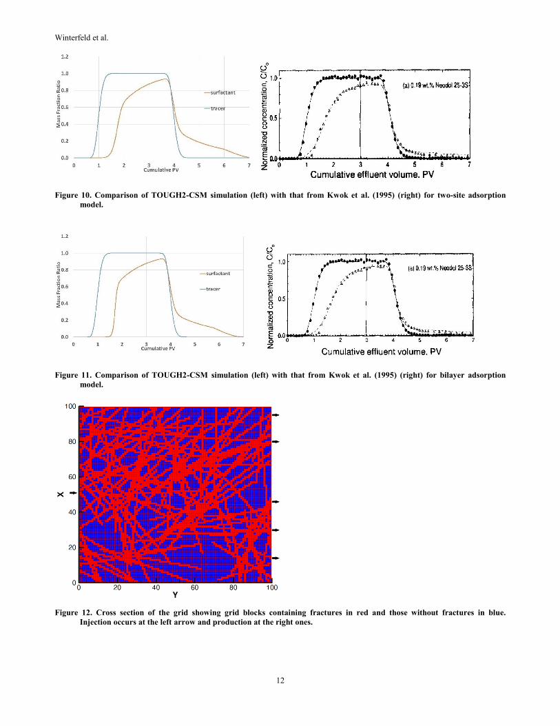
Winterfeld et al
15
Figure 17 Thermal breakthrough simulations for various injection rates for above case