
Code deisgn for SISO and MIMO block-fading channels882/fulltext.pdf · CODE DEISGN FOR SISO AND...
124
CODE DEISGN FOR SISO AND MIMO BLOCK-FADING CHANNELS A Dissertation Presented by Yueqian Li to The Department of Electrical and Computer Engineering in partial fulfillment of the requirements for the degree of Doctor of Philosophy in Communications and Digital Signal Processing Northeastern University Boston, Massachusetts April 2013
Transcript of Code deisgn for SISO and MIMO block-fading channels882/fulltext.pdf · CODE DEISGN FOR SISO AND...

CODE DEISGN FOR SISO AND MIMO BLOCK-FADING CHANNELS
A Dissertation Presented
by
Yueqian Li
to
The Department of Electrical and Computer Engineering
in partial fulfillment of the requirements
for the degree of
Doctor of Philosophy
in
Communications and Digital Signal Processing
Northeastern University
Boston, Massachusetts
April 2013

c© Copyright by Yueqian Li 2013
All Rights Reserved
ii

NORTHEASTERN UNIVERSITY
Graduate School of Engineering
Dissertation Title: CODE DEISGN FOR SISO AND MIMO BLOCK-FADING CHAN-
NELS
Author: Yueqian Li
Department: Electrical and Computer Engineering
Approved for Dissertation Requirement for the Doctor of Philosophy Degree
Dissertation Advisor Professor Masoud Salehi Date
Dissertation Reader Professor Milica Stojanovic Date
Dissertation Reader Professor Kaushik Chowdhury Date
Dissertation Reader Date
Department Chair Professor Ali Abur Date
Graduate School Notified of Acceptance:
Director of the Graduate School Date
iii

Abstract
We study, analyze, and design communication systems for data transmission over block-
fading channels. The block-fading channel is a model for communication under slowly-
varying fading; where a codeword spans a few independent fading blocks. Code design
strategies for block-fading channels are quite different from those for classical additive white
Gaussian noise (AWGN) channels or fully interleaved fading channels.
From the expression for pairwise error probability (PEP) bound under maximum likeli-
hood (ML) decoding, we can extract two major parameters for code design on block-fading
channels; the diversity order and the coding gain. At high signal to noise ratios, the diver-
sity order determines the slope of the codeword error probability curve, while the coding
gain shifts the curve horizontally. Therefore, the diversity order is the determining factor
in code design. The optimal diversity order achievable by coding scheme is upper bounded
by the Singleton bound, which establishes the fundamental tradeoff between coding rate
and diversity order. The family of codes which can achieve the optimal diversity order are
referred as blockwise maximum distance separable (MDS) codes. The general approach for
code construction on block-fading channels is to design MDS codes with large coding gain.
For single-input single-output (SISO) communication, we propose a blockwise convo-
lutionally encoded bit-interleaved coded modulation (BC-BICM) scheme, which achieves
optimal diversity order. In addition, the coding gain can be improved either by choosing
a carefully designed signal labeling scheme for the BICM with iterative decoding or by
using convolutional codes with longer constraint lengths. We also investigate quasi-cyclic
low-density parity-check (QC-LDPC) codes for block-fading channels. With careful design,
the proposed QC-LDPC codes exhibit the same good performance as their corresponding
random root-LDPC codes. Moreover, the structure of the proposed QC-LDPC codes makes
them suitable for efficient encoding.
For the multiple-input multiple-output (MIMO) situation, the system design should
iv
take advantage of additional space diversity provided by multiple antennas besides the time
diversity. We first study a turbo coded BICM scheme with iterative detection. The signal
processing unit at the receiver employs sphere detector to achieve good performance with
reduced computation complexity. To obtain the full diversity of the channel, we propose a
coded space-time scheme based on modulation diversity, where the channel coding exploits
the time diversity and space-time coding provides space diversity. It is shown that the
proposed system achieves high throughput by transmitting at full spatial multiplexing.
v

Acknowledgements
First and foremost, I would like to express my sincere appreciation and gratitude to my
advisor, Prof. Masoud Salehi, for his guidance and support during my doctoral studies.
He has been a great source of knowledge to this work. I have learned a lot through our
discussions and it is a real pleasure to work with him. I feel very lucky to have him as my
PhD advisor.
I am grateful to Prof. Milica Stojanovic and Prof. Kaushik Chowdhury for accepting
to be members of my thesis committee, and providing valuable feedbacks on the draft of
this dissertation. I own many thanks to them for their time and effort in helping me with
my research work.
During my PhD program, I took two internships, which have greatly enriched my ex-
perience and been benefit to my future career. I would like to thank those mentors who
hosted me in their teams, including Dr. Sean Ramprashad, Dr. Sayandev Mukherjee and
Dr. Haralabos Papadopoulos from DOCOMO Communications Labs USA and Dr. Toshiaki
Koike-Akino from Mitsubishi Electric Research Laboratories (MERL).
I also would like to thank my friends at Northeastern University for their friendship.
They have made my study at Northeastern University more enjoyable. In particular, I am
thankful to the members of Communications and Digital Signal Processing (CDSP) center.
It is a great honor for me to be part of CDSP and it is a great experience to work with
those talented people in CDSP center.
Finally, I am indebted to my family. It would not have been possible to finish this
doctoral dissertation without the support and encouragement from the family. I especially
wish to express my gratitude to my wife, Ran, for her love and support.
This dissertation is dedicated to my parents and my wife.
vi

Contents
Abstract iv
Acknowledgements vi
1 Introduction 1
1.1 The Block-Fading Channel Model . . . . . . . . . . . . . . . . . . . . . . . . 3
1.2 The Information Outage Limits . . . . . . . . . . . . . . . . . . . . . . . . . 4
1.3 Code Design . . . . . . . . . . . . . . . . . . . . . . . . . . . . . . . . . . . . 7
1.3.1 The Pairwise Error Probability . . . . . . . . . . . . . . . . . . . . . 8
1.3.2 The Singleton Bound and MDS Code . . . . . . . . . . . . . . . . . 11
1.3.3 Coding for Block-Fading Channels . . . . . . . . . . . . . . . . . . . 12
1.4 MIMO Block-Fading Channels . . . . . . . . . . . . . . . . . . . . . . . . . 13
1.4.1 The MIMO Systems . . . . . . . . . . . . . . . . . . . . . . . . . . . 13
1.4.2 The MIMO Block-Fading Channel Model . . . . . . . . . . . . . . . 23
1.5 Research Contributions . . . . . . . . . . . . . . . . . . . . . . . . . . . . . 26
2 A New BC-BICM Scheme for Block-Fading Channels 27
2.1 Blockwise Convolutional Codes for Block-Fading
Channels . . . . . . . . . . . . . . . . . . . . . . . . . . . . . . . . . . . . . 27
2.2 System Model . . . . . . . . . . . . . . . . . . . . . . . . . . . . . . . . . . . 29
2.3 BC-BICM with Improved Coding Gain . . . . . . . . . . . . . . . . . . . . . 31
2.3.1 Symbol Labeling for BC-BICM with Iterative Decoding . . . . . . . 31
2.3.2 Convolutional Codes with Longer Constraint Lengths . . . . . . . . 33
2.4 Comparison between BC-BICM and BCC-BICM . . . . . . . . . . . . . . . 34
2.5 Conclusions . . . . . . . . . . . . . . . . . . . . . . . . . . . . . . . . . . . . 36
vii

3 Quasi-Cyclic LDPC Code Design for Block-Fading Channels 37
3.1 Linear Block and LDPC Codes . . . . . . . . . . . . . . . . . . . . . . . . . 38
3.1.1 Linear Block Codes . . . . . . . . . . . . . . . . . . . . . . . . . . . 38
3.1.2 LDPC Codes . . . . . . . . . . . . . . . . . . . . . . . . . . . . . . . 38
3.1.3 QC-LDPC Codes . . . . . . . . . . . . . . . . . . . . . . . . . . . . . 39
3.2 QC-LDPC Code Design for Block-Fading Channels . . . . . . . . . . . . . . 40
3.2.1 Root-LDPC Codes . . . . . . . . . . . . . . . . . . . . . . . . . . . . 40
3.2.2 Construction of QC-LDPC Codes . . . . . . . . . . . . . . . . . . . . 41
3.2.3 QC-LDPC Codes with Large Girth . . . . . . . . . . . . . . . . . . . 43
3.3 Simulation Results . . . . . . . . . . . . . . . . . . . . . . . . . . . . . . . . 45
3.4 Efficient Encoding Method . . . . . . . . . . . . . . . . . . . . . . . . . . . . 48
3.5 Conclusions . . . . . . . . . . . . . . . . . . . . . . . . . . . . . . . . . . . . 49
4 Turbo Coded BICM Scheme with Iterative Detection for MIMO Block-
Fading Channels 50
4.1 System Model of Turbo Coded BICM Scheme . . . . . . . . . . . . . . . . . 51
4.1.1 Transmitter Structure in Parallel Concatenated Turbo Coded BICM 51
4.1.2 Transmitter Structure for Serial Concatenated Turbo Coded BICM . 52
4.1.3 Iterative Detection . . . . . . . . . . . . . . . . . . . . . . . . . . . . 53
4.2 The Array Processing Method . . . . . . . . . . . . . . . . . . . . . . . . . . 55
4.3 Sphere Decoder with Max-Log MAP Performance . . . . . . . . . . . . . . . 57
4.4 K-Best Sphere Decoding with Fixed Complexity . . . . . . . . . . . . . . . 62
4.5 Simulation results . . . . . . . . . . . . . . . . . . . . . . . . . . . . . . . . 64
4.5.1 Performance of sphere decoder . . . . . . . . . . . . . . . . . . . . . 64
4.5.2 Comparison between serial and parallel turbo codes . . . . . . . . . 68
4.6 Conclusions . . . . . . . . . . . . . . . . . . . . . . . . . . . . . . . . . . . . 71
5 Coded MIMO Systems with Modulation Diversity for Block-Fading
Channels 72
5.1 Space-Time Coding Based on Modulation Diversity . . . . . . . . . . . . . . 73
5.2 System Model of Coded MIMO System Based on Modulation Diversity . . 77
5.2.1 Transmitter Structure . . . . . . . . . . . . . . . . . . . . . . . . . . 77
5.2.2 Receiver with Iterative Detection . . . . . . . . . . . . . . . . . . . . 78
5.3 Simulation Results . . . . . . . . . . . . . . . . . . . . . . . . . . . . . . . . 81
viii
5.4 Conclusions . . . . . . . . . . . . . . . . . . . . . . . . . . . . . . . . . . . . 86
6 An Efficient Decoding Algorithm for Concatenated RS-Convolutional Codes 87
6.1 Introduction . . . . . . . . . . . . . . . . . . . . . . . . . . . . . . . . . . . . 87
6.2 The Reed-Solomon Codes . . . . . . . . . . . . . . . . . . . . . . . . . . . . 88
6.2.1 The RS Code Encoding . . . . . . . . . . . . . . . . . . . . . . . . . 89
6.2.2 Decoding of RS Codes . . . . . . . . . . . . . . . . . . . . . . . . . . 90
6.3 The RS-Convolutional Concatenated Coding Scheme . . . . . . . . . . . . . 94
6.4 A Low Complexity Decoding Algorithm . . . . . . . . . . . . . . . . . . . . 95
6.5 Simulation Results . . . . . . . . . . . . . . . . . . . . . . . . . . . . . . . . 98
6.6 Conclusions . . . . . . . . . . . . . . . . . . . . . . . . . . . . . . . . . . . . 100
7 Concluding remarks and future work 101
7.1 Concluding remarks . . . . . . . . . . . . . . . . . . . . . . . . . . . . . . . 101
7.2 Future work . . . . . . . . . . . . . . . . . . . . . . . . . . . . . . . . . . . . 103
Bibliography 104
ix
List of Tables
6.1 The decoding procedure for RS codes. . . . . . . . . . . . . . . . . . . . . . 93
6.2 Error patterns of flipping 3 bits. . . . . . . . . . . . . . . . . . . . . . . . . 98
x

List of Figures
1.1 A codeword of length N spans over F = 2 fading blocks. . . . . . . . . . . . 4
1.2 Outage limits of a block-fading channel with F = 2 using complex Gaussian
inputs. . . . . . . . . . . . . . . . . . . . . . . . . . . . . . . . . . . . . . . . 6
1.3 Outage limits of block-fading channels with F = 2, 4, 8, and 16 using complex
Gaussian inputs, R = 1 bit/sec/Hz. . . . . . . . . . . . . . . . . . . . . . . . 7
1.4 The transmitter structure of VBLAST. . . . . . . . . . . . . . . . . . . . . . 18
1.5 Receiver block diagram for VBLAST using ZF-SIC. . . . . . . . . . . . . . 21
1.6 Outage probabilities for MIMO block-fading channels with assumption of
Gaussian inputs and genie-aided detector. . . . . . . . . . . . . . . . . . . . 25
2.1 The encoder structure of (5, 3, 7, 7) convolutional code. . . . . . . . . . . . 28
2.2 Minimum blockwise Hamming distance path for a block-fading channel with
F = 8. . . . . . . . . . . . . . . . . . . . . . . . . . . . . . . . . . . . . . . . 28
2.3 The transmitter structure of the BC-BICM scheme. . . . . . . . . . . . . . 29
2.4 The receiver structure of the BC-BICM scheme. . . . . . . . . . . . . . . . . 30
2.5 16-QAM labeling schemes: Gray, SP, MSP. . . . . . . . . . . . . . . . . . . 32
2.6 WER of the BC-BICM scheme obtained by BP decoding of 10 iterations over
independent Rayleigh block-fading channel with F = 4. . . . . . . . . . . . 33
2.7 WER of the BC-BICM scheme with different convolutional codes obtained by
BP decoding of 10 iterations over independent Rayleigh block-fading channel. 34
2.8 WER of the BCC-BICM scheme and BC-BICM scheme obtained by BP
decoding of 10 iterations over independent Rayleigh block-fading channel
with F=4. . . . . . . . . . . . . . . . . . . . . . . . . . . . . . . . . . . . . . 35
3.1 A rate rc = 1/2 regular (3, 6) root-LDPC code for a block-fading channel
with F = 2. . . . . . . . . . . . . . . . . . . . . . . . . . . . . . . . . . . . . 40
xi

3.2 Illustration of construction of QC-root-LDPC Codes. . . . . . . . . . . . . . 42
3.3 An example of length-4 cycle in QC LDPC codes. . . . . . . . . . . . . . . . 44
3.4 FER performance comparison for QC root LDPC codes, random root LDPC
codes, random LDPC codes and ML designed LDPC codes over a block-
fading channel with F = 2. . . . . . . . . . . . . . . . . . . . . . . . . . . . 45
3.5 FER performance comparison of QC-root-LDPC codes with girth 2g = 4, 6
and 8 over a block-fading channel with F = 2. . . . . . . . . . . . . . . . . . 46
3.6 FER and BER performance of QC-root-LDPC codes with codeword length
N = 160, 1200 and 8000 over a block-fading channel with F = 2. The
number of iterations is 20. . . . . . . . . . . . . . . . . . . . . . . . . . . . . 47
4.1 Block diagram of the parallel concatenated turbo coded BICM transmitter. 52
4.2 Block diagram of the serial concatenated turbo coded BICM transmitter. . 53
4.3 Block diagram of the receiver with iterative detection and decoding. . . . . 53
4.4 Geometrical interpretation of sphere decoding. . . . . . . . . . . . . . . . . 58
4.5 Sphere decoding search tree for BPSK constellation with Nt = 4. . . . . . . 60
4.6 FER performance comparison between sphere decoding and array processing
over a block-fading channel with F = 2. . . . . . . . . . . . . . . . . . . . . 65
4.7 Average number of nodes visited during the sphere decoding search in a 4×4
MIMO block-fading channel with F = 2. . . . . . . . . . . . . . . . . . . . . 66
4.8 FER performance comparison between sphere decoding (both max-log and
K-best) and array processing over a 4× 4 MIMO block-fading channel with
F = 2. . . . . . . . . . . . . . . . . . . . . . . . . . . . . . . . . . . . . . . . 67
4.9 FER performance comparison between sphere decoding (both max-log and
K-best) and array processing over a 8× 8 MIMO block-fading channel with
F = 2. . . . . . . . . . . . . . . . . . . . . . . . . . . . . . . . . . . . . . . . 68
4.10 FER performance for parallel and serial concatenated turbo coded BICM
scheme with Nt = 2 and QPSK modulation. . . . . . . . . . . . . . . . . . . 69
4.11 FER performance for parallel and serial concatenated turbo coded BICM
scheme in both SISO and MIMO block-fading channels. . . . . . . . . . . . 70
5.1 The threaded layers in space-time code scheme with Nt = 3. . . . . . . . . . 76
5.2 Transmitter structure of the coded MIMO system. . . . . . . . . . . . . . . 77
5.3 Block diagram of the receiver with iterative detection and decoding. . . . . 78
xii

5.4 FER performance of the coded MIMO system over a 2×1 MIMO quasi-static
fading channel. . . . . . . . . . . . . . . . . . . . . . . . . . . . . . . . . . . 82
5.5 FER performance of the coded MIMO system over MIMO block-fading chan-
nels with F = 2 fading blocks. . . . . . . . . . . . . . . . . . . . . . . . . . . 83
5.6 Average number of nodes visited during the sphere decoding search in a 2×2
MIMO block-fading channel with F = 2 fading blocks. . . . . . . . . . . . . 84
5.7 Comparison of FER performance between the coded MIMO system and the
serically Turbo-coded BICM scheme with Nt = 2, Nr = 2, over MIMO block-
fading channels of F = 2 fading blocks. . . . . . . . . . . . . . . . . . . . . . 85
6.1 The block diagram RS/Conv concatenated coding scheme. . . . . . . . . . . 94
6.2 BER performance of the concatenated RS/Conv coding system. . . . . . . . 99
6.3 Complexity comparison between proposed algorithm and Chase algorithm. . 100
xiii

Chapter 1
Introduction
Mobile communication techniques have evolved dramatically in recent years; mainly due to
the increasing demand for high quality and fast wireless data service. The wireless channel
is considered to be one of the most challenging channel models for reliable communications.
The main impairments present in a wireless communication environment include noise,
fading, and interference, which pose major challenges in designing effective and reliable
communication systems for mobile users.
The deteriorating effect of fading is one of the most challenging problems encountered
by the designer of wireless communication systems. The effects of fading can generally be
classified into large scale fading (noticeable over distances much larger than the wavelength)
and small scale fading [1]. Large scale fading is mainly due to path loss and shadowing
whereas small scale fading is a result of multipath propagation of electromagnetic waves
and their reflection and scattering from nearby objects. In this research, we only consider
the effects of small scale fading. Because the received signal is the sum of a large number
of reflections of the transmitted signal (diffuse component), by applying the central limit
theorem we can conclude that the amplitude of the received signal is a Rayleigh distributed
random variable. When there exists a line-of-sight component (specular component), the
amplitude of the received signal is modeled as a Ricean distributed random variable.
Another property of wireless channels is that their characteristics change with time.
This is mainly due to mobility of transmitter and/or receiver, as well as variations in the
transmission environment. The coherence time Tc of a fading channel is defined as the time
duration during which the channel impulse response does not change. Therefore, the value
of the coherence time of the channel characterizes how rapidly the channel changes with
1

CHAPTER 1. INTRODUCTION 2
time. The coherence time is inversely related to the Doppler spread fd [1]
Tc ≈1
fd. (1.1)
In (1.1), fd is the maximum Doppler shift given by fd = v/λ = fcvc , where v, c, fc and λ
are the relative velocity between transmitter and receiver, the velocity of light, the carrier
frequency, and the carrier wavelength, respectively. When the coherence time is less than
the symbol period, the channel is refereed as a fast fading channel. When the coherent time
is larger than the symbol (or the codeword) duration, the channel is refereed as a slow fading
channel. Two convenient models that are widely used in the study of wireless channels are
the quasi-static and fully interleaved fading channel models. In the quasi-static fading
channel model, it is assumed that the fading coefficient is constant for an entire codeword
duration and changes independently from one codeword to another. For fully interleaved
fading channel model, we assume that the codeword passes through a long interleaver prior
to transmission and hence the codeword spans a relatively long time interval, which is
much longer than the coherence time. In this case, the fading coefficients are different and
independent for every transmitted bit.
In this dissertation, we investigate the problem of wireless data transmission over a
more realistic fading channel model, i.e., the block-fading channel model. In this channel
model, a single codeword may span a few fading blocks with independent fading coefficients.
The quasi-static and fully interleaved fading channel models can be considered as the two
extreme cases of the block-fading channel. The block-fading channel model is a general
and convenient model for delay sensitive communications over wireless links affected by
slow-varying fading. The block-fading channel model is an appropriate channel model for
the following situations:
• Slow frequency hopping: A codeword is divided into segments, which are sent on
different frequency bands. The purpose of slow frequency hopping is to provide di-
versity for transmission links. Systems that employ slow frequency hopping include
Global System for Mobile communications (GSM) and Enhanced Data rates for GSM
Evolution (EDGE) [2].
• Hybrid Automatic Repeat reQuest (HARQ) with incremental redundancy (IR): When
the initial transmission fails, the subsequent retransmissions contain different coded
CHAPTER 1. INTRODUCTION 3
bits from the initial transmission. The transmissions are sent on different transmis-
sion time intervals (TTIs) with independent interference levels. Systems that employ
HARQ with IR, include High Speed Packet Access (HSPA), 3GPP Long Term Evolu-
tion (LTE) [3, 4], and worldwide interoperability for microwave access (WiMAX) [5].
• Cooperative communication: A codeword is sent in parts by the original node and the
cooperative partner relay nodes. As those nodes are distributed at different locations,
the fading coefficients for those parts are independent [6].
The selection of communication system architecture and system parameters in general
depends on channel conditions. An off-the-shelf scheme designed for additive white Gaussian
noise (AWGN) channel, quasi-static fading channel, or fully interleaved channel may not
perform well over a block-fading channel. In fact, the design rules for block-fading channels
are quite different from those for such classic channels. In this chapter, we first provide
preliminaries on the block-fading channel, including the mathematical model for the channel
and information outage limits. Then, error correcting code design criteria for block-fading
channels are discussed. Some existing communication systems for block-fading channels are
introduced.
We also discuss how to improve the performance of the communication over block-
fading channels using multiple-input multiple-output (MIMO) techniques. At the end of
this chapter, we summarize the contributions of the dissertation.
1.1 The Block-Fading Channel Model
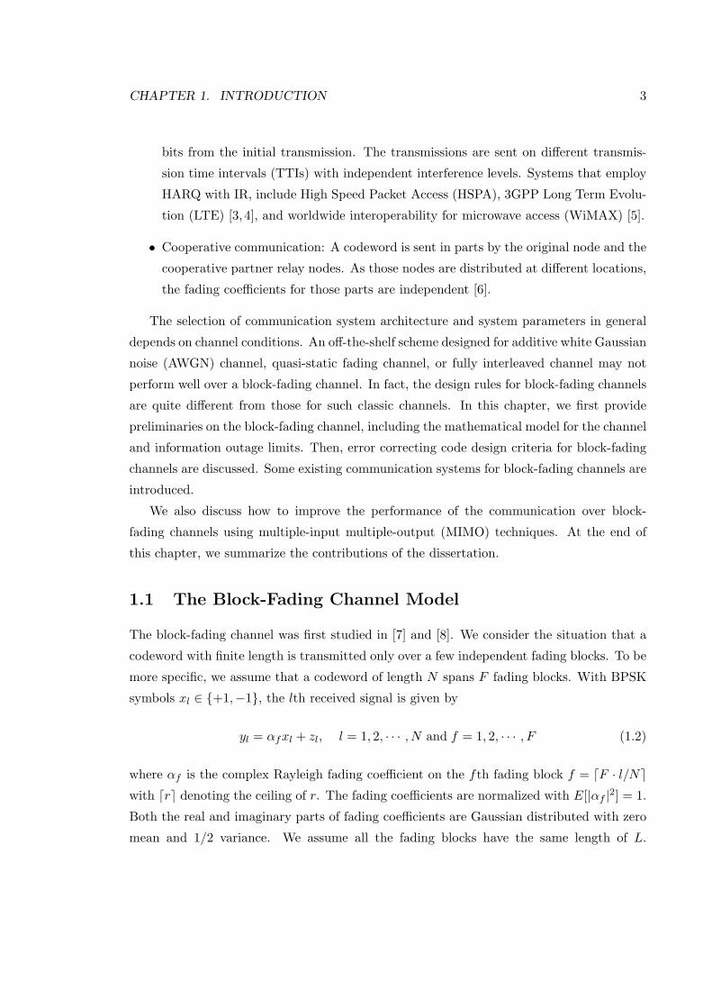
The block-fading channel was first studied in [7] and [8]. We consider the situation that a
codeword with finite length is transmitted only over a few independent fading blocks. To be
more specific, we assume that a codeword of length N spans F fading blocks. With BPSK
symbols xl ∈ +1,−1, the lth received signal is given by
yl = αfxl + zl, l = 1, 2, · · · , N and f = 1, 2, · · · , F (1.2)
where αf is the complex Rayleigh fading coefficient on the fth fading block f = ⌈F · l/N⌉with ⌈r⌉ denoting the ceiling of r. The fading coefficients are normalized with E[|αf |2] = 1.
Both the real and imaginary parts of fading coefficients are Gaussian distributed with zero
mean and 1/2 variance. We assume all the fading blocks have the same length of L.

CHAPTER 1. INTRODUCTION 4
Therefore, FL = N . The noise is sampled from a zero mean circularly symmetric complex
Gaussian variable with variance σ2 = N0/2 per each dimension. The signal-to-noise ratio
(SNR) is expressed as Eb/N0, where Eb is the energy per information bit. A simple example
of a codeword in a block-fading channel with F = 2 fading blocks is illustrated in Fig. 1.1.
1 2
A codeword of length N
Figure 1.1: A codeword of length N spans over F = 2 fading blocks.
When QAM symbols from constellation X of size 2Q are used, a frame is referred as a
symbol sequence of length N/Q mapped from a codeword of length N . In this situation,
the block length is L = N/(F ·Q).
1.2 The Information Outage Limits
The capacity of a communication channel is defined as the highest rate at which the in-
formation can be reliably transmitted over the channel. Since the channel gain of a fading
channel is random, the instantaneous channel capacity is also a random variable. For a
fast fading channel, we assume the channel changes fast enough and a single codeword can
experience all possible realizations of the channel. In this case, the ergodic channel capac-
ity is defined as the ensemble average of channel capacity over all states of the channel.
The word “ergodic” infers the assumption that the time average of instantaneous channel
capacity within a codeword duration equals to statistical average of channel capacity. For
slow fading channels including block-fading channels, different codewords will experience
different realizations of the channel. Thus, the channel capacity changes for each codeword
transmission. Instead of using ergodic capacity, information outage limit and outage capac-
ity are defined to measure the slow fading channel quality, which are detailed in the rest of
this section for block-fading channels.
Due to the nonergodic nature of the block-fading channel, its Shannon capacity is zero,
which means reliable transmission of information at any positive rate is impossible over this
channel. There is a certain probability that the current channel condition cannot support
the loading transmission rate R, which describes that situation that the channel is in outage.

CHAPTER 1. INTRODUCTION 5
The channel is characterized by its information outage limit, also called outage probability,
which is defined as
Pout = Pr(I(Eb/N0, αf) < R), (1.3)
where I(Eb/N0, αf) is the instantaneous mutual information between the input and the
output of the channel. The value of the instantaneous mutual information depends on
current SNR and channel condition αf. R = (K/N)×Q = rc×Q denotes the transmission
rate, where K is the number of information bits and rc = K/N is the code rate. The outage
limit (1.3) is the ultimate lower bound on frame error rate (FER) for any coding scheme
over block-fading channels. With real Gaussian input and a throughput of R information
bits per dimension, the instantaneous mutual information is calculated by
IGr(Eb/N0, αf) =1
F
F∑
j=1
1
2log2
(1 + 2R
Eb
N0|αf |2
). (1.4)
With complex Gaussian input and a throughput of R information bits per complex dimen-
sion, the instantaneous mutual information is calculated by
IGc(Eb/N0, αf) =1
F
F∑
j=1
log2
(1 +R
Eb
N0|αf |2
). (1.5)
With BPSK inputs, the corresponding instantaneous mutual information does not have
a closed form and it is given by [9, p. 363]
IBPSK(Eb/N0, αf)
=1
F
F∑
f=1
1
2·(g
(√2R
Eb
N0|αf |2
)+ g
(−√2R
Eb
N0|αf |2
)),
(1.6)
where
g(t) =
∫ ∞
−∞
1√2π
e−(w−t)2
2 log22
1 + e−2wtdw. (1.7)
The above function is symmetric g(t) = g(−t) and the value of g(t) can be computed using
the Gauss-Hermite quadrature method.
For general complex QAM inputs, the instantenous mutual information can be calculated

CHAPTER 1. INTRODUCTION 6
as [2]
IQAM (Eb/N0, αf) =1
F
F∑
f=1
IQAM (Eb/N0, αf ), (1.8)
where
IQAM (Eb/N0, αf ) = Q− 2−Q∑
x∈X
E
[log2
∑
x′∈X
exp(−|αf
√REb
N0(x− x′)|2 + |Z|2)
]. (1.9)
In above equation the expectation is taken with respect to the circular complex noise Z ∼NC(0, 1) and the value of the expectation can also be evaluated by the Gauss-Hermite
quadrature method.
Fig. 1.2 shows outage limits of a block-fading channel with F = 2 using complex Gaus-
sian inputs. The channel loads are set to be R = 0.5, 1, 2 and 3 bits/complex dimension.
We can see that the outage curves shift to right when the channel load R increases. We
observe that all outage limit curves have the same slop of 2 at high SNR region, which is
the diversity order of the channel.
0 5 10 15 20 2510
−4
10−3
10−2
10−1
100
Eb/No (dB)
Ou
tag
e P
out
R = 0.5 bit/sec/Hz
R = 1 bit/sec/Hz
R = 2 bit/sec/Hz
R = 3 bit/sec/Hz
Figure 1.2: Outage limits of a block-fading channel with F = 2 using complex Gaussianinputs.

CHAPTER 1. INTRODUCTION 7
Fig. 1.3 illustrates outage limits of block-fading channels with F = 2, 4, 8, and 16. We
fix the channel load at R = 1 bit / complex dimension and assume complex Gaussian inputs
are used. For the same system load, we get steeper outage curves with more fading blocks.
0 2 4 6 8 10 12 14 16 18 2010
−5
10−4
10−3
10−2
10−1
100
Eb/No (dB)
Ou
tag
e P
out
F = 2
F = 4
F = 8
F = 16
Figure 1.3: Outage limits of block-fading channels with F = 2, 4, 8, and 16 using complexGaussian inputs, R = 1 bit/sec/Hz.
Another channel quality indicator is the outage capacity defined as the highest trans-
mission rate that can be supported by the channel without exceeding the pre-set outage
limit ǫ ∈ [0, 1)
Cǫ = maxR : Pout(R) < ǫ. (1.10)
In this dissertation, we will only use the outage limit as performance criterion for coding
system designs.
1.3 Code Design
The goal of channel code design is to match code structure to channel conditions. Code
design criteria are different for different channel conditions. For example, over a binary

CHAPTER 1. INTRODUCTION 8
symmetric channel (BSC) with cross probability less than 0.5, a good code should have a
large minimum Hamming distance. Similarly, for an AWGN channel, the design rule is to
maximize the minimum Euclidean distance.
Code design criteria for block-fading channels have been discussed in various works
including [2, 10,11]. In this section, we briefly review the design rules based on asymptotic
analysis. In the high SNR region, the average FER, also known as codeword error rate
(WER), for the block-fading channel can be expressed as
Pe ≈ Gc · (SNR)−d. (1.11)
From (1.11), we can see that the FER, in the high SNR region, is determined by two
parameters, d and Gc, where d is referred to as the diversity order and Gc is known as the
coding gain. By taking the logarithm of both sides of (1.11), we have
log(Pe)≈− d · log(SNR) + log(Gc). (1.12)
The diversity order determines the asymptotic slope of the error probability curve as a
function of SNR on a log-log scale, while the coding gain provides a horizontal shift in the
curve.
1.3.1 The Pairwise Error Probability
We begin by considering a block-fading channel with independent Ricean fading coefficients
on each fading block. We further assume the energy of the fading coefficient is normalized,
i.e., E(|αf |2) = S2+2σ2 = 1, where S2 and 2σ2 is the specular and the diffuse components,
respectively. For this channel model, the Rice factor is defined as KRice = S2
2σ2 . When
KRice = 0, we have a Rayleigh fading channel with 2σ2 = 1. When KRice → ∞, we have
a Gaussian channel with S2 = 1. We assume that the message m consisting of binary
coded bits of length N is mapped onto the symbol sequence x(m) and is transmitted over
the channel spanning F independent fading realizations. The conditional pairwise error
probability (PEP) between two codewords x(m) and x(m′) under maximum likelihood (ML)
decoding can be expressed as
Pe
(x(m) → x(m′)|αf
)= Q
√√√√F∑
f=1
|αf |2d2f (x(m), x(m′))
2N0
, (1.13)

CHAPTER 1. INTRODUCTION 9
where
d2f (x(m), x(m′)) =L∑
l=1
|x(f−1)L+l(m)− x(f−1)L+l(m′)|2 (1.14)
is the squared Euclidean distance between the portions of two codewords on fading block
f . The Q function in (1.13) is referred as Gaussian tail probability function and defined as
Q(x) = P [N (0, 1) > x] =1
2π
∫ ∞
xexp(− t2
2)dt.
By averaging the channel conditional pairwise error probability with channel distribu-
tion, we obtain the average pairwise error probability
Pe (x(m) → x(m′))
/1
2
F∏
f=1
KRice + 1
KRice + 1 +d2f(x(m),x(m′))
4N0
exp
−KRice
d2f(x(m),x(m′))
4N0
KRice + 1 +d2f(x(m),x(m′))
4N0
.
(1.15)
A detailed derivation of the average pairwise error probability over the distribution of
αf random variables by using moment-generating function of Chi-squared distribution is
given in [10]. A similar result for the fully interleaved Ricean fading channel can be found
in [9, Sec. 14.4]. We examine two special cases of Rayleigh block-fading channel and AWGN
channel by setting KRice = 0 and letting KRice → ∞.
• KRice = 0: average PEP for Rayleigh block-fading channel
Pe
(x(m) → x(m′)
)≤ 1
2
F∏
f=1
1
1 +d2f(x(m),x(m′))
4N0
(1.16)
• KRice → ∞: average PEP for AWGN channel
Pe (x(m) → x(m′)) ≤ 1
2
F∏
f=1
exp
(−d2f (x(m), x(m′))
4N0
)
=1
2exp
(−d2(x(m), x(m′))
4N0
),
(1.17)
where d2(x(m), x(m′)) is the squared Euclidean distance between symbol sequences
mapped from two codewords.
CHAPTER 1. INTRODUCTION 10
To obtain the average PEP over the codewords, we can apply the union bound
Pe ≤∑
m
∑
m′ 6=m
P (x(m))Pe
(x(m) → x(m′)
)
≤∑
m
∑
m′ 6=m
1
2Nmaxm,m′
Pe
(x(m) → x(m′)
)
= (2N − 1) ·maxm,m′
Pe
(x(m) → x(m′)
)
(1.18)
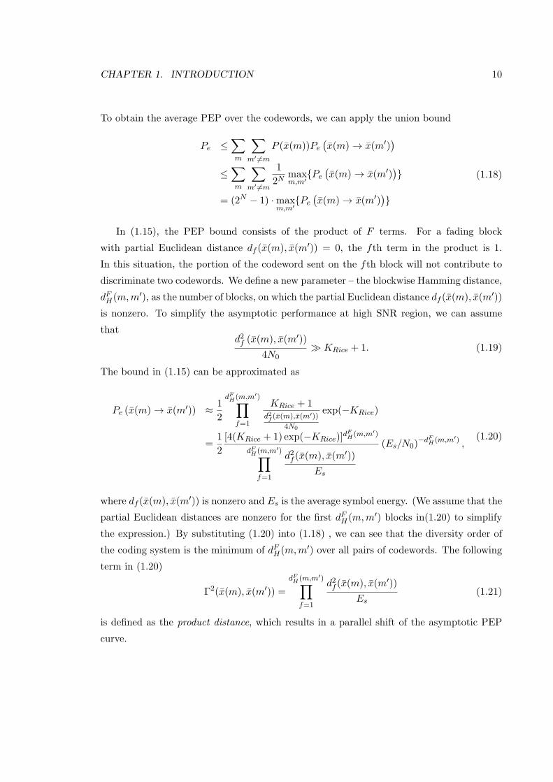
In (1.15), the PEP bound consists of the product of F terms. For a fading block
with partial Euclidean distance df (x(m), x(m′)) = 0, the fth term in the product is 1.
In this situation, the portion of the codeword sent on the fth block will not contribute to
discriminate two codewords. We define a new parameter – the blockwise Hamming distance,
dFH(m,m′), as the number of blocks, on which the partial Euclidean distance df (x(m), x(m′))
is nonzero. To simplify the asymptotic performance at high SNR region, we can assume
thatd2f (x(m), x(m′))
4N0≫ KRice + 1. (1.19)
The bound in (1.15) can be approximated as
Pe (x(m) → x(m′)) ≈ 1
2
dFH(m,m′)∏
f=1
KRice + 1d2f(x(m),x(m′))
4N0
exp(−KRice)
=1
2
[4(KRice + 1) exp(−KRice)]dFH(m,m′)
dFH(m,m′)∏
f=1
d2f (x(m), x(m′))
Es
(Es/N0)−dFH(m,m′) ,
(1.20)
where df (x(m), x(m′)) is nonzero and Es is the average symbol energy. (We assume that the
partial Euclidean distances are nonzero for the first dFH(m,m′) blocks in(1.20) to simplify
the expression.) By substituting (1.20) into (1.18) , we can see that the diversity order of
the coding system is the minimum of dFH(m,m′) over all pairs of codewords. The following
term in (1.20)
Γ2(x(m), x(m′)) =
dFH(m,m′)∏
f=1
d2f (x(m), x(m′))
Es(1.21)
is defined as the product distance, which results in a parallel shift of the asymptotic PEP
curve.

CHAPTER 1. INTRODUCTION 11
The diversity order is clearly the determining parameter in the design of error correcting
codes for block-fading channels. The error correcting codes designed for a block-fading
channel are expected to exploit the limited diversity orders that the channel provides and
at the same time achieve good coding gain.
1.3.2 The Singleton Bound and MDS Code
For a block code C with codeword length N , information length K and the minimum
distance d, the Singleton bound states that
d ≤ N −K + 1 = N(1− rc) + 1. (1.22)
The Singleton bound can be modified to bound blockwise Hamming distance for code design
in block-fading channels.
Theorem 1.3.1 (Singleton Bound). The achievable diversity order on a block-fading chan-
nel with F blocks is bounded by the Singleton bound [10,11]:
d ≤ ⌊F (1− rc)⌋+ 1, (1.23)
where rc (≤ 1) is the code rate and ⌊x⌋ represents the the largest integer smaller than or
equal to x.
Equation (1.23) clearly reflects the optimal trade-off between code rate rc and diversity
order d.
Proof. Let L denote the length of a fading block. It is convenient to view L symbols over a
fading block together as a super-symbol XL [7]. With this interpretation of super-symbols,
the analysis of block-fading channels is reduced to the analysis of a non-binary block code
with symbols in the form of XL with a fixed codeword length F . The diversity order of
the coding system is equal to the minimum Hamming distance among all the codewords.
Furthermore, all traditional bounding techniques can be applied to analyze the coding
system for the block-fading channels.
The class of error correcting codes, which can achieve the Singleton bound on block-
fading channels, are referred to as blockwise maximum distance separable (MDS) codes.
CHAPTER 1. INTRODUCTION 12
However, most existing MDS codes cannot be used on block-fading channels directly, be-
cause the codeword length is constrained to be F with typical value of 2 ∼ 8, which is
generally too short for a codeword.
It has been shown in [10, 12, 13] that the the maximal diversity order F is achieved
by outage limit using Gaussian inputs; the optimal diversity order given by the Singleton
bound is achieved by outage limit using a finite size QAM constellation.
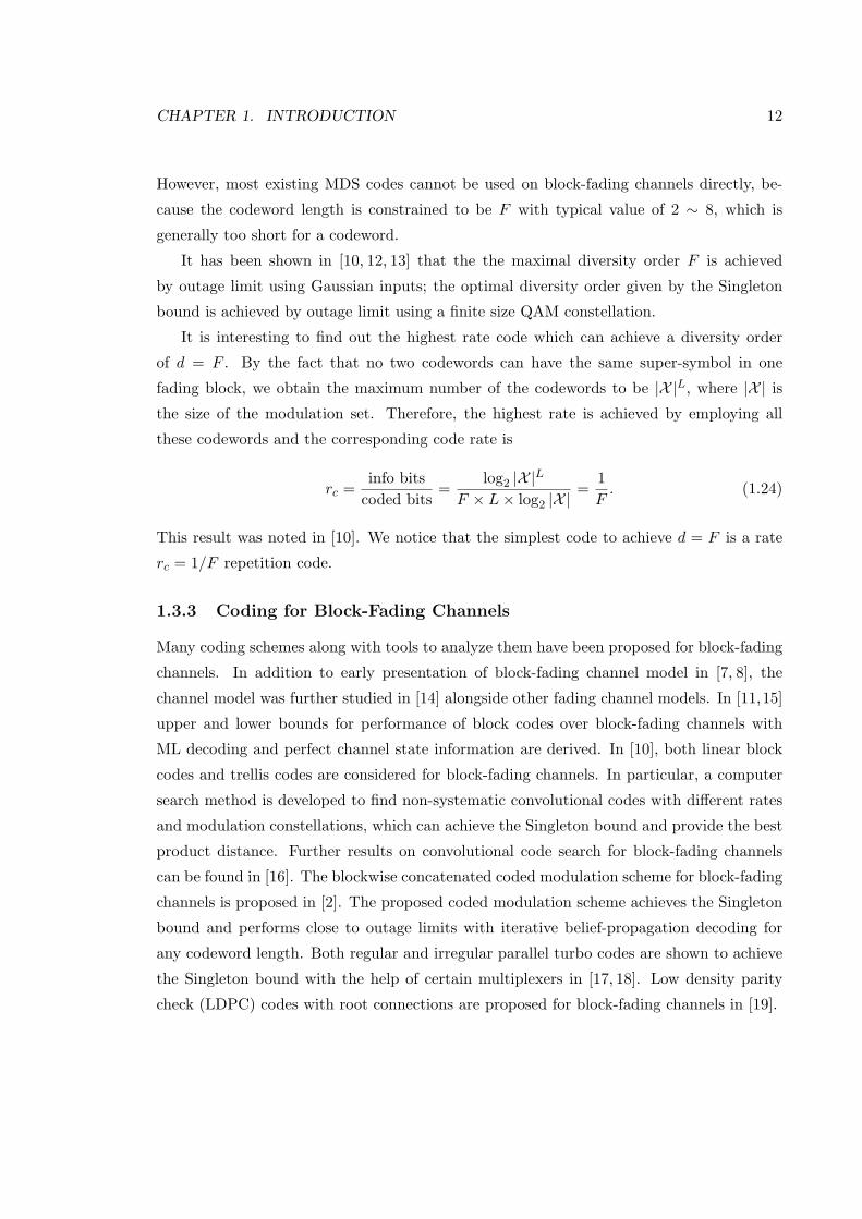
It is interesting to find out the highest rate code which can achieve a diversity order
of d = F . By the fact that no two codewords can have the same super-symbol in one
fading block, we obtain the maximum number of the codewords to be |X |L, where |X | isthe size of the modulation set. Therefore, the highest rate is achieved by employing all
these codewords and the corresponding code rate is
rc =info bits
coded bits=
log2 |X |LF × L× log2 |X | =
1
F. (1.24)
This result was noted in [10]. We notice that the simplest code to achieve d = F is a rate
rc = 1/F repetition code.
1.3.3 Coding for Block-Fading Channels
Many coding schemes along with tools to analyze them have been proposed for block-fading
channels. In addition to early presentation of block-fading channel model in [7, 8], the
channel model was further studied in [14] alongside other fading channel models. In [11,15]
upper and lower bounds for performance of block codes over block-fading channels with
ML decoding and perfect channel state information are derived. In [10], both linear block
codes and trellis codes are considered for block-fading channels. In particular, a computer
search method is developed to find non-systematic convolutional codes with different rates
and modulation constellations, which can achieve the Singleton bound and provide the best
product distance. Further results on convolutional code search for block-fading channels
can be found in [16]. The blockwise concatenated coded modulation scheme for block-fading
channels is proposed in [2]. The proposed coded modulation scheme achieves the Singleton
bound and performs close to outage limits with iterative belief-propagation decoding for
any codeword length. Both regular and irregular parallel turbo codes are shown to achieve
the Singleton bound with the help of certain multiplexers in [17, 18]. Low density parity
check (LDPC) codes with root connections are proposed for block-fading channels in [19].
CHAPTER 1. INTRODUCTION 13
1.4 MIMO Block-Fading Channels
Communication systems designed for block-fading channels are expected to achieve both
high diversity order and good coding gain [10]. Since the diversity order is limited by
channel intrinsic diversity orders in block-fading channels, we consider employing MIMO
techniques to provide additional spatial diversity. Another important advantage of using
multiple antennas is to enable high rate transmission through spatial multiplexing. Diversity
coding can be used together with spatial multiplexing, where transmission reliability is in
tradeoff with the system throughput.
1.4.1 The MIMO Systems
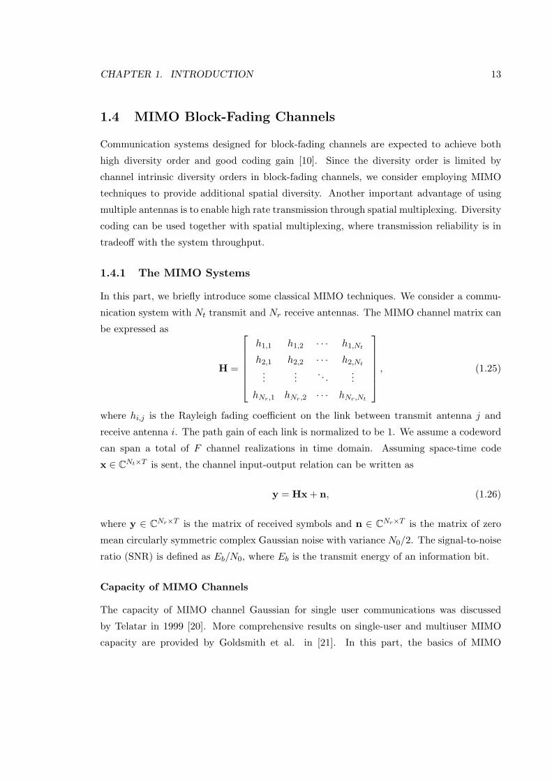
In this part, we briefly introduce some classical MIMO techniques. We consider a commu-
nication system with Nt transmit and Nr receive antennas. The MIMO channel matrix can
be expressed as
H =
h1,1 h1,2 · · · h1,Nt
h2,1 h2,2 · · · h2,Nt
......
. . ....
hNr,1 hNr ,2 · · · hNr,Nt
, (1.25)
where hi,j is the Rayleigh fading coefficient on the link between transmit antenna j and
receive antenna i. The path gain of each link is normalized to be 1. We assume a codeword
can span a total of F channel realizations in time domain. Assuming space-time code
x ∈ CNt×T is sent, the channel input-output relation can be written as
y = Hx+ n, (1.26)
where y ∈ CNr×T is the matrix of received symbols and n ∈ C
Nr×T is the matrix of zero
mean circularly symmetric complex Gaussian noise with variance N0/2. The signal-to-noise
ratio (SNR) is defined as Eb/N0, where Eb is the transmit energy of an information bit.
Capacity of MIMO Channels
The capacity of MIMO channel Gaussian for single user communications was discussed
by Telatar in 1999 [20]. More comprehensive results on single-user and multiuser MIMO
capacity are provided by Goldsmith et al. in [21]. In this part, the basics of MIMO

CHAPTER 1. INTRODUCTION 14
channel capacity for single user case are reviewed. To simplify the representation, we
assume a single use of the deterministic MIMO channel. Following the Telatar’s approach,
we can decompose MIMO channel into a set of parallel SISO channels by singular value
decomposition (SVD) of channel matrix
H = UΛVH , (1.27)
where U and V are two complex unitary matrices, Λ is an Nr × Nt rectangular diagonal
matrix with real nonnegative sigular values λi on the diagonal. By left-multiplying UH to
both sides of (1.27), we have
y = Λx+ n, (1.28)
where y = UHy, x = VHx and n = UHn. The new noise vector n is still white and its
power is unchanged, as U is a unitary matrix. The number of the independent parallel
channels is determined by the rank k of the channel matrix H. When the channel state
information (CSI) is available at the transmitter, the capacity is achieved by waterfilling the
available transmit power P over those parallel channels with power gains given by λ2i [22].
The resulting channel capacity is given by
CCSITMIMO =
k∑
i=1
log2
(1 +
Piλ2i
N0
), (1.29)
where Pi = (µ− N0
λ2i
)+ is the power filled into channel i. The water level µ is choosen to to
satisfy the total power constraint P =∑k
i=1 Pi.
Capacity without CSIT At High SNR At the high SNR region, we have a huge
amount of power. In this situation, we will use all available parallel channels and it is
asymptotically optimal to fill equal amounts of power to those channels. The channel
capacity can be expressed as
CCSITMIMO /
k∑
i=1
log2
(1 +
Pλ2i
kN0
). (1.30)
The condition number (eigenvalue spread) of the channel matrix H is defined as the ratio
between the largest and smallest eigenvalue values (maxλi/minλi). The channel is said

CHAPTER 1. INTRODUCTION 15
to be well-conditioned, if the condition number is close to 1. In this situation, the capacity
is achieve by equal power allocation. If the channel is full rank, we have k = minNt, Nrand the MIMO capacity linearly increases as k · log(SNR) at the high SNR region. This
result is refereed as degree-of-freedom gain in [23].
Capacity with CSIT At Low SNR At the low SNR region, we have a small amount
of power and the optimal strategy is to fill all available power to the channel with largest
channel gain. The resulting channel capacity is
CCSITMIMO / log2
(1 +
P maxλ2i
N0
). (1.31)
For small value x, we have the approximation log2(1 + x) ≈ x log2 e by Taylor expansion
around 0. And the capacity in (1.31) can be approximated by
CCSITMIMO ≈ P maxλ2
i N0
log2 e = maxλ2i SNR log2 e. (1.32)
The MIMO system provides a power gain of maxλ2i with low SNR [23].
Capacity without CSIT When channel state information or statistical properties of the
channel is not available at the transmitter, we will allocate equal amount of power to each
transmit antenna. The capacity of MIMO channel without CSI at the transmitter is
Cno−CSITMIMO = log2 det
(INr +
P
NtN0HHH
). (1.33)
Similarly, we decompose HHH = UΛ2UH . The capacity in (1.33) can the expressed as
Cno−CSITMIMO = log2 det
(INr +
PNtN0
Λ2)
=
k∑
i=1
log2
(1 +
Pλ2i
NtN0
),
(1.34)
where k is the rank of the channel matrix H .

CHAPTER 1. INTRODUCTION 16
Space-Time Block Codes
Space-time block codes (STBC) based on orthogonal designs are able to achieve full space
diversity with low-complexity receiver at the expense of low rate (no more than 1 symbol
per channel use) [24]. The very first and simplest STBC design with two transmit antennas
and a single receive antennas was invented by Alamouti in 1998 [25]. The transmitted
codeword of Alamouti scheme is
x =
[x1,1 x1,2
x2,1 x2,2
]=
[s1 −s∗2
s2 s∗1
], (1.35)
where s1 and s2 are symbols selected from any signal constellation. We assume the MIMO
channel matrix
H = [h1 h2] (1.36)
is constant for two consecutive channel use. The received symbols for two transmission are
y1 = h1s1 + h2s2 + n1
y2 = −h1s∗2 + h2s
∗1 + n2
. (1.37)
The maximum-likelihood (ML) decoding of Alamouti scheme can be decoupled into two
independent parts
s1 = argmins1
(|h1|2 + |h2|2 − 1
)|s1|+ |s1 − y1h
∗1 − y∗2h2|2
s2 = argmins2
(|h1|2 + |h2|2 − 1
)|s2|+ |s2 − y1h
∗2 + y∗2h1|2
. (1.38)
Following the similar decoding procedure above, we actually decode each symbol separately
for general STBC codes. Therefore the ML decoding complexity for STBC codes grows
linearly, instead of exponentially, with the number of transmit antennas. It can be shown
that the received signal SNR is the sum of SNRs on two links
SNR =(|h1|2 + |h2|2)Es
N0, (1.39)
where Es is average transmitted symbol energy of the signal constellation [26].
The Alamouti coding scheme can be generalized with more than two transmit antennas
based on orthogonal designs [24]. Two attractive features of STBC are:

CHAPTER 1. INTRODUCTION 17
• low-complexity ML decoding: each symbol can be decoded separately;
• the ability to provide full diversity: the code based on orthogonal designs satisfies
rank criterion [24].
Spatial Multiplexing and Receiver Architectures
Instead of utilizing the multiple transmit antennas for additional diversity gain, we may
increase the transmission rate by sending different data steams on different transmit an-
tennas. The has been shown the capacity of MIMO system increases linearly with the
number of transmit antennas, when the number of receive antennas is equal to the number
of transmit antennas [27]. Layered space-time codes allow spatial multiplexing to increase
the transmission rate with reduced diversity, based on the general framework of Bell Lab-
oratories Layered Space-Time (BLAST) architectures [28]. However, it is not possible to
have a simpler ML decoder to detect each symbol separately as STBC codes. Sub-optimal
and low-complexity receiver designs are necessary for spatial multiplexing to work in prac-
tice. We take vertical BLAST (V-BLAST) as an example and briefly discuss several receiver
architectures for spatial multiplexing.
The transmitter structure of VBLAST is draw in Fig. 1.4. First, the bit stream is
mapped into symbol stream. Then, the symbol stream is demultiplexed into Nt substreams
and emitted from the corresponding transmit antenna. Assuming there is no additional
temporal channel coding, each receive antenna will receive all Nt symbols from all transmit
antennas at the receiver. The input and output relation for a single transmission can be
represent as
y = Hx + n , (1.40)
where x is the transmitted symbol vector of size Nt and y is the received signal vector of
size Nr.
A detector which is capable to suppress the interference and separate those signals should
be employed. The algorithms are pretty much the same as those developed for multiuser
detection (MUD) [29].
ML Detector The ML detector processes all Nt symbols jointly by searching over all
possible transmitted symbol vectors. With circularly symmetric complex Gaussian noise n ,

CHAPTER 1. INTRODUCTION 18
NtBitstream...
Figure 1.4: The transmitter structure of VBLAST.
the ML detector choose the symbol vector, which minimizes the following metric
x = argminx
||Hx − y ||2F , (1.41)
where ||·||F is Frobenius norm. The ML detector is optimal in terms of minimizing the
probability of decoding a codeword in error. When the constellation size is 2M , the num-
ber of candidate vectors is 2MNt , which grows exponentially with the number of transmit
antennas. Therefore, it is impractical to perform ML decoding with a large number of
transmit antennas. Suboptimal low-complexity linear equalization techniques can be used
to distinguish symbols.
Zero-Forcing (ZF) Detector The zero-forcing equalizer tries to find the inverse of the
channel matrix, which completely eliminates the intersymbol interference (ISI). In case
that H is full rank square matrix, we have WZF = H−1. For general situation, we can use
Moore-Penrose pseudo-inverse (left inverse) of the channel as the Zero-forcing coefficients
WZF = H+ =(HHH
)−1HH , (1.42)
where HH denotes the conjugate transpose of the channel matrix H. Multiplying H+ with
1.40 results in
x = WZFy = H+y = y +H+n . (1.43)
After the zero-forcing equalization, we could decoder each symbol separately by finding the
nearest point in the constellation to the corresponding element in x . The ZF equalization
requires Nr ≥ Nt to work. As shown in (1.43), the disadvantage of using zero-forcing

CHAPTER 1. INTRODUCTION 19
equalization is to enhance the noise power by a factor of
H+(H+)H
=((
HHH)−1
HH)((
HHH)−1
HH)H
=(HHH
)−1. (1.44)
When noise power is small (near zero), ZF is a good choice to suppress ISI. A more balanced
linear filter is a linear minimum mean square error (MMSE) equalizer, which provides a
trade-off between suppressing the interference and enhancing the noise.
Linear MMSE detector In general, the MMSE detector provides a conditional mean
estimation for x based on observation y
x = E [x |y ] , (1.45)
which minimize minimize mean square error (MSE) E[(x − x )2
]. However, it is usually
difficult to calculate the close-form MMSE detector. One solution is to restrict the estimator
to be linear, i.e., x = Wy . And the linear MMSE detector equalizer tries to find the
coefficients WMMSE to minimize following term
E[(WMMSEy − x )(WMMSEy − x )H
]. (1.46)
The linear MMSE filter coefficients can be derived by orthogonality principle
E[(x − x )yH
]= E
[(WMMSEy − x )yH
]= 0
E [(x − x )] = E [(WMMSEy − x )] = 0, (1.47)
which is actually the necessary and sufficient condition for optimality in general MMSE
sense. As the mean values of x and y are both zero vectors, we ignore the second condition
of the orthogonality principle. From the first condition, we get
WMMSER = HH · Px, (1.48)
where Px = E[xix∗i ] is the average transmit symbol power and R is Nr×Nr autocorrelation
matrix of received vector y
R = E[yyH
]=[HHH · Px + INr ·N0
]. (1.49)

CHAPTER 1. INTRODUCTION 20
Therefore, the linear MMSE estimator
WMMSE = Px ·HHR−1 = HH
[HHH + INr ·
N0
Px
]−1
=
[HHH+ INt ·
N0
Px
]−1
HH , (1.50)
where the equivalent form in the last step is obtained using Woodbury matrix identity.
Decision Feedback Equalization (DFE) In contrast to ML detector, which possesses
symbols jointly, the aforementioned two linear equalization approaches multiply the received
vector with a matrix and then decodes each symbol separately. These symbol-by-symbol
style detectors reduce the system processing complexity at the cost of reduced performance.
A decision feedback equalizer improves the performance of a linear detector by using pre-
vious detector decisions to eliminate the interference.
If the symbols are processed successively, the previous detected symbols can be sub-
tracted from received signal to aid the detection of the next symbol. The method is ref-
ereed as successive interference cancellation or serial interference cancellation (SIC), which
was originally proposed for multi-user detection (MUD) [30]. The problem of SIC is the
excessive detection delay, as the algorithm processes each layer serially. Multistage par-
allel interference cancellation (PIC) was proposed as an alternative for SIC to reduce the
processing delay, in which the interference is simultaneously removed from all layers [31].
The original detection method for VBLAST is based on SIC with optimal ordering [28].
The algorithm first decodes the strongest layer. Assuming the successful detection of this
strongest layer, the interference effect of this layer can be canceled from all of the receiver
equations. Then, the second strongest layer is detected and its effects are removed from all
equations before the detection of the next layer. The process continues until the last layer
is detected. The block diagram of ZF-SIC equalizer is depicted in Fig. 1.5.
The algorithm starts with ordering the signals by their post-detection SNR. For ZF
equalization, the post-detection SNR for layer-i can be expressed as
SNRi =Pi
N0|wi|2, (1.51)
where |wi|2 is the norm of ith row vector from ZF equalization matrix WZF (1.42). For
equal power case, the ordering is dependent on the value of norm of nulling vector wi, which
acts as a noise enhance factor in ZF equalization. After (l− 1) layers have been processed,
their interference will be removed from the received signal. We have new input-output

CHAPTER 1. INTRODUCTION 21
ZF
Equalization
ZF
Equalization
Layer 1
Cancellation
of Layer 1
Layer 2
Cancellation
of Layer 2
ZF
Equalization
Layer Nt
y
Cancellation
of Layer Nt-1
Figure 1.5: Receiver block diagram for VBLAST using ZF-SIC.

CHAPTER 1. INTRODUCTION 22
relation at the lth stage
yl = Hlxl + n = y − Il = [hl, hl+1, · · ·hNt ]xl + n, (1.52)
where xl contains (Nt − (l − 1)) undetected signals and Il is the reconstructed interference
from detected signals. We need to recalculate ZF equalization matrix according to (1.52) and
start the process again. The ZF-SIC detection algorithm can be summarized as following 3
steps:
• Ordering by post-detection SNR values;
• Interference nulling by ZF equalization;
• Interference reconstruction and cancellation.
It is interesting to point out that the diversity oder achieved by each layer is different by
its detection order. For ZF equalization, it is required that Nr should be no less than Nt.
The diversity gain is (Nr −Nt + 1) for the first detected layer and Nr for the last detected
layer. The reason of diversity gain difference is that ZF equalization uses receive diversity
to nullify the interference.
Precoding Techniques for MIMO
If channel state information is available at the transmitter side through feedback, precoding
can be performed combined with spatial multiplexing (multi-layer beamforming) to maxi-
mize the MIMO system throughput. The major difference between precoding and conven-
tional beamforming (smart antennas) is that the precoding enables multi-layer transmission
and beamforming supports only signal-layer transmission.
For point-to-point communication, singular value decomposition (SVD) precoding is the
optimal following the similar analysis for capacity of single user deterministic MIMO channel
[20]. Multiple streams are precoded with a unitary matrix and emitted from all available
transmit antennas. At the receiver side, another unitary matrix is multiplied to received
vector to detected all transmitted symbols. In this circumstance, each non-zero singular
value act as a parallel channel without interference and can support an independent data
stream. In addition, the channel capacity is achieved with water filling power allocation.
The precoding technique for multi-user communication is adopted by multi-user MIMO
(MU-MIMO) to support multiple access, which is an extended concept of space-division

CHAPTER 1. INTRODUCTION 23
multiple access (SDMA). It is known that non-linear Dirty Paper Coding (DPC) is optimal
precoding, which can pre-cancel known interference at the transmitter [32, 33]. As the
complexity with non-linear precoding is high, it is preferable to adopt linear precoding
strategies in practical applications [34].
Due to their attractive performance, MIMO techniques have been adopted by almost all
modern wireless communication standards, including UMTS HSPA and LTE [3, 4], IEEE
802.16e WiMAX [5] and IEEE 802.11n WLAN [35]. We will consider several MIMO tech-
niques and corresponding signal processing techniques in our research to take advantage of
their diversity gain and spatial multiplexing.
1.4.2 The MIMO Block-Fading Channel Model
In this model, the channel matrix H is constant over L transmissions and changes inde-
pendently for next L transmissions. We assume a codeword can span a total of F channel
realizations in time domain. We also assume that the transmit antennas and the receive
antennas are separated far enough in space, so that the fading coefficients between each
transmit-receive pair are independent.
The Channel Model
At time t, a vector x(t) = [x1(t), x2(t), · · · , xNt(t)] is transmitted over the Nt transmit
antennas. We assume the symbol energy is normalized to 1, i.e., E(|xj(t)|2) = 1. A vector
y(t) = [y1(t), y2(t), · · · , yNr(t)] is received at the Nr receive antennas. The received vector
y(t) can be expressed as
y(t) = H(t)x(t) + n(t), (1.53)
where n(t) = [n1(t), n2(t), · · · , nNr(t)] is the zero mean circularly symmetric complex Gaus-
sian noise vector with each element of variance N0/2 per dimension. The system signal to
noise ratio (SNR) is measured by Eb/N0, where Eb is the transmit energy per information
bit.
We follow the assumption in [13] that when we detect the signal from the transmit
antenna j at receive antenna i, a genie provides the knowledge of symbols from other
transmit antennas. In this way, we can convert MIMO channel into a set of single-input

CHAPTER 1. INTRODUCTION 24
single output (SISO) non-interfering parallel block-fading channels,
yi,j(t) = hi,j(t)xj(t) + ni(t). (1.54)
This assumption is valid when we are able to detect interferences from other transmit
antennas and cancel them successfully. With this assumption, we can apply both coding
schemes and analysis method designed for SISO block-fading channels to the MIMO cases.
For example,
The Outage Limits
The Shannon capacity of the nonergodic MIMO block-fading channel is zero. As in SISO
case, we characterize the channel by its information outage limit, which is defined as
Pout = Pr (I(Eb/N0,H) < R) , (1.55)
where I(Eb/N0,H) is the instantaneous mutual information between the input and the
output of the MIMO channel and R = rc ×M ×Nt is the system loading rate, where rc is
the coding rate and 2M is the modulation constellation size.
Assuming the CSI is unknown at the transmitter side, the power is equally allocated to
each fading block. The instantaneous mutual information is calculated as
IG(Eb/N0,H) =
Nt∑
j=1
[1
F
F∑
k=1
log2(1 + SNRk,j)
], (1.56)
where
SNRk,j = rc ×M × (Eb/N0)
Nr∑
i=1
|hi,j(L× k)|2. (1.57)
In (1.56), we assume complex Gaussian input is used and Shannon capacity formula is
adopted. The SNR value is calculated according to a practical communication system with
certain coding and modulation configuration as shown in (1.57). Several outage limits with
versus Eb/N0 are drawn in Fig.1.6. The spectral efficiency is R = 1 bits/transmission for
Nt = 1 and R = 2 bits/transmission for Nt = 2. The Fig.1.6 shows that we will get curves
with steeper slop, when the number of antennas or the number of fading blocks increases.
The season is that the available diversity order determines the slope of the outage probability

CHAPTER 1. INTRODUCTION 25
curve with Gaussian input in the high SNR region. For F = 2, the maximum achievable
diversity order is just 2 in the SISO case. Using 2 × 2 MIMO, we can achieve a diversity
order of 8 over an F = 2 block-fading channel. For the case Nt = 1, Nr = 1, F = 2 and the
case Nt = 2, Nr = 1, F = 1, the outage limits are the same.
−5 0 5 10 15 2010
−5
10−4
10−3
10−2
10−1
100
Eb/No (dB)
Ou
tag
e P
out
Nt=1 Nr=1 F=2
Nt=2 Nr=1 F=1
Nt=2 Nr=1 F=2
Nt=2 Nr=1 F=4
Nt=2 Nr=2 F=2
d=8
d=8
d=4
d=2
Figure 1.6: Outage probabilities for MIMO block-fading channels with assumption of Gaus-sian inputs and genie-aided detector.
The achievable diversity order d by a coding scheme for MIMO block-fading channels is
upper-bounded by the modified Singleton bound
d ≤ Nr (⌊FNt(1− rc)⌋+ 1) . (1.58)
The internal part ⌊FNt(1−rc)⌋+1 in (1.58) can be viewed as the diversity order provided by
a SISO block-fading channel with F ×Nt independent fading blocks. The receive diversity
order Nr is achieved by maximum ratio combining.
CHAPTER 1. INTRODUCTION 26
1.5 Research Contributions
In this dissertation, we focus on the communication system designs for data transmission
over block-fading channels. The block-fading channel model is a channel model for delay
sensitive communication over slow-varying wireless link, where a codeword experiences a
few independent fading blocks. We review code design criteria for the block-fading channel
through the analysis of PEP performance bound under ML decoding. Two major param-
eters are diversity order and coding gain. Therefore, the code design approach is to find
blockwise MDS codes with good coding gain.
Our first design is a BC-BICM scheme for SISO block-fading channels. Compared with
BCC-BICM scheme, the proposed scheme also achieves the Singleton bound but has less
delay in both encoding and decoding. We can improve the the coding gain of BC-BICM
scheme through proper design of signal mapping scheme or using a strong convolutional
code. Then, we study a QC-LDPC scheme, whose parity check matrices are designed using
circulant matrices. The QC-LDPC achieves the same good performance as its corresponding
root-LDPC scheme. The structure of the QC-LDPC code enables efficient encoding.
For MIMO cases, we investigated both serial and parallel concatenated turbo coded bit-
interleaved coded modulation (BICM) schemes. The two schemes are compared in terms
of performance in MIMO block-fading channels. In addition, a sphere decoder is used as a
practical low-complexity signal processing solution, when the number of transmit antennas
or the size of modulation constellation is large. The sphere decoder offers better perfor-
mance compared with the group suppression technique. However, the achievable diversity
order is not guaranteed with serial and parallel concatenated turbo coded BICM schemes.
The systems designed for SISO case cannot be used directly in MIMO block-fading chan-
nels to achieve optimal diversity order because of the interference introduced by multiple
transmitting antennas. To solve the diversity problem, a coded MIMO system based on
modulation diversity technique is proposed. The scheme achieves both full spatial multi-
plexing and full diversity of NtNrF , i.e., the product of the number of transmit antennas
Nt, receive antennas Nr and fading blocks F . The drawback of modulation diversity is
the increased complexity at the detector. We show how to employ a sphere decoder in the
proposed system to reduce the signal processing complexity.

Chapter 2
A New BC-BICM Scheme for
Block-Fading Channels
In this chapter, we introduce and study a blockwise convolutional coded bit-interleaved
coded modulation (BC-BICM) scheme for the class of block-fading channels. The proposed
BC-BICM scheme can be viewed as a simplified version of the blockwise concatenated con-
volutional coded bit-interleaved coded modulation (BCC-BICM) scheme [2], which achieves
the Singleton bound as long as the blockwise partitioned outer code is a MDS code. Further-
more, we improve the coding gain by choosing better symbol mapping rules with iterative
detection of BICM [36, 37] or using stronger convolutional codes. Simulations results are
provided to confirm the effectiveness of our approach.
2.1 Blockwise Convolutional Codes for Block-Fading
Channels
Non-recursive convolutional codes for block-fading channels are studied in [10, 16], where
MDS convolutional codes with large product distance (coding gain) are designed using
computer search techniques. We illustrate the search principle by an example. The coding
rate of the example convolutional code is rc = 1/4 with generator G = (5, 3, 7, 7) in octal
form. The encoder structure is shown in Fig. 2.1. The rate-1/4 code has 4 output taps
and the coded bits from those taps are blockwisely partitioned according to the number of
fading blocks. We assume that BPSK modulation is employed. For a block-fading channel
27

CHAPTER 2. BC-BICM SCHEME 28
of 8 fading blocks, two input information bits will generate 8 coded bits, which are sent to
8 fading blocks repectively as illustrated in Fig. 2.1.
on block 1 and 5
on block 2 and 6
on block 3 and 7
on block 4 and 8
Figure 2.1: The encoder structure of (5, 3, 7, 7) convolutional code.
Because convolutional codes are linear, the distance property of a convolutional code
can be studied by using the all-zero codeword as a reference. The trellis diagram of the
code is illustrated in Fig. 2.2.
00 00 00 00 00 00
01 01 01
10 10 10
11 11
1/1011
0/01
11
0/11
11
0/0000 0/0000 0/0000 0/0000 0/0000
1/1100
1/0011
0/10
00
0/11
11
Block 1~4 Block 5~8 Block 1~4 Block 5~8 Block 1~4
1/1011
mindH = 10
min = 6 F
Hd
F = 8
Figure 2.2: Minimum blockwise Hamming distance path for a block-fading channel withF = 8.
For a block-fading channel of F = 8 fading blocks, the maximum achievable diversity
is 7 with a rate rc = 1/4 code, which is given by the Singleton bound (1.23). However,
the example code only provides a diversity order of dFH = 6. The path with minimum
blockwise Hamming distance is illustrated by red dotted arrows. For comparison, we also
show the path corresponding to minimum Hamming distance (minimum free distance) by
CHAPTER 2. BC-BICM SCHEME 29
blue solid arrows. From the example, we can see that the minimum Hamming distance path
and the minimum blockwise Hamming distance are not necessarily the same path. The
Hamming distance property of the convolutional code can be characterized by its transfer
function [38]. The minimum blockwise Hamming distance can only be found using computer
search, because it is also depended on the number of fading blocks. Convolutional codes
with good blockwise Hamming distance for different values of F are found by computer
search [10, 16].
2.2 System Model
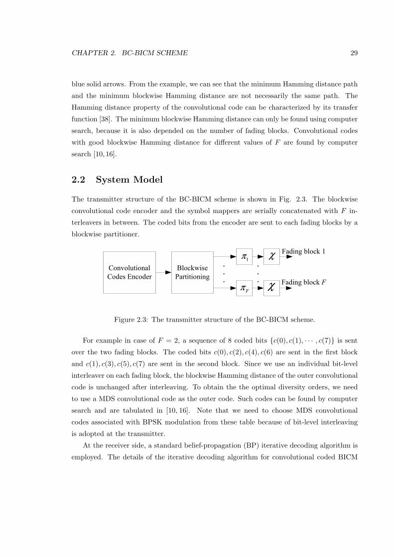
The transmitter structure of the BC-BICM scheme is shown in Fig. 2.3. The blockwise
convolutional code encoder and the symbol mappers are serially concatenated with F in-
terleavers in between. The coded bits from the encoder are sent to each fading blocks by a
blockwise partitioner.
Convolutional
Codes Encoder
Blockwise
Partitioning
1π.
.
.
Fπ
χ
χ
Fading block 1
Fading block F
.
.
.
Figure 2.3: The transmitter structure of the BC-BICM scheme.
For example in case of F = 2, a sequence of 8 coded bits c(0), c(1), · · · , c(7) is sent
over the two fading blocks. The coded bits c(0), c(2), c(4), c(6) are sent in the first block
and c(1), c(3), c(5), c(7) are sent in the second block. Since we use an individual bit-level
interleaver on each fading block, the blockwise Hamming distance of the outer convolutional
code is unchanged after interleaving. To obtain the the optimal diversity orders, we need
to use a MDS convolutional code as the outer code. Such codes can be found by computer
search and are tabulated in [10, 16]. Note that we need to choose MDS convolutional
codes associated with BPSK modulation from these table because of bit-level interleaving
is adopted at the transmitter.
At the receiver side, a standard belief-propagation (BP) iterative decoding algorithm is
employed. The details of the iterative decoding algorithm for convolutional coded BICM

CHAPTER 2. BC-BICM SCHEME 30
can be found in [36]. The channel decoder uses the BCJR algorithm [39] and the symbol
demapper uses maximum a posteriori (MAP) algorithm. The extrinsic information is ex-
changed between the symbol demapper and the decoder via de-interleaver/interleaver, just
like the decoding of process serially concatenated turbo codes. The receiver structure is
illustrated in Fig. 2.4.
Decoder
(BCJR)Demapper
Received
sequence
1
Figure 2.4: The receiver structure of the BC-BICM scheme.
The ith received signal from a fading block with coefficient αf can be expressed as
yi = αfxi + ni, (2.1)
where ni is the noise. The transmitted symbol xi is from a signal constellation X of size 2M
and each symbol conveys M coded bits. Let us denote coded bits by c = [c1, c2, · · · , cM ].
The a posteriori log-likelihood ratio (LLR) value for the lth coded bit can be calculated as
λ(cl) = logPr[cl = 1|yi, αf ]
Pr[cl = 0|yi, αf ]= log
Pr[cl = 1, yi|αf ]
Pr[cl = 0, yi|αf ]
= log
∑
c:cl=1
Pr[yi, c|αf ]
∑
c:cl=0
Pr[yi, c|αf ]
= log
∑
c:cl=1
Pr[yi|c, αf ]Pr(c)
∑
c:cl=0
Pr[yi|c, αf ]Pr(c).
(2.2)
Under the condition of perfect interleaving, we have Pr(c) =∏M
j=1 Pr(cj), which indicates

CHAPTER 2. BC-BICM SCHEME 31
those coded bits are independent. In this situation, (2.2) can be expressed as
λ(cl) = log
∑
c:cl=1
Pr[yi|c, αf ]
M∏
j=1
Pr(cj)
∑
c:cl=0
Pr[yi|c, αf ]
M∏
j=1
Pr(cj)
. (2.3)
Equation (2.2) shows the a posteriori LLR value of coded bit cl. The a priori LLR
value from convolutional code decoder is
LLR(cl) = logPr(cl) = 0
Pr(cl) = 1. (2.4)
The extrinsic information e(cl) generated by symbol demapper is calculated by subtracting
(2.4) from (2.2)
e(cl) = log
∑
c:cl=1
Pr[yi|c, αf ]Pr(c)
∑
c:cl=0
Pr[yi|c, αf ]Pr(c)− log
Pr(cl) = 0
Pr(cl) = 1, (2.5)
which is the input to the BCJR decoder.
2.3 BC-BICM with Improved Coding Gain
In this section, we propose two methods to improve the coding gain of the BC-BICM scheme.
In the first method, we improve the performance of the modulation part by employing
better symbol labeling schemes. Then, we improve the performance of coding part by
using convolutional codes with longer constraint lengths. Simulation results are provided
to demonstrate the effectiveness of these methods.
2.3.1 Symbol Labeling for BC-BICM with Iterative Decoding
Gray mapping is the best labeling method for non-iterative decoding of convolutionally
coded BICM, because Gray labeling has the fewest number of nearest neighbors for the
decision of each bit in each position regardless of its position in the coded sequence. However,
the performance of Gray mapping is not as good when used in an iterative decoding scheme.

CHAPTER 2. BC-BICM SCHEME 32
With an optimized signal labeling scheme, the feedback soft bits can enlarge the conditional
intersignal Euclidean distance, which leads to a larger coding gain [36, 37, 40].
R
I
1111
0101000110011101
0100000010001100
0110001010101110
011100111011
(a) Gray mapping
R
I
1000
0010011101100011
0101000000010100
1110101110101111
100111001101
(b) SP mapping
R
I
1000
1010100111101101
0011000001110100
0110010100100001
111111001011
(c) MSP mapping
(Minimum SED = 1) (Minimum SED = 1) (Minimum SED = 2)
Figure 2.5: 16-QAM labeling schemes: Gray, SP, MSP.
In the high SNR region, we can assume that the demapper receives ideal soft information
about the coded bits from the feedback provided by the decoder. Therefore, the demapper
can decide the value of each coded bit by considering only two signal points in the signal
constellation. Hence the error performance is dominated by the conditional intersignal
squared Euclidean distance (SED). The general labeling design rule is to find a constellation
with optimized minimum conditional intersignal SED. Computer search results of optimized
signal labeling for 8-PSK and 16-QAM constellations are given in [36, 40]. The 16-QAM
constellation with Gray, set partitioning (SP), and modified set partitioning (MSP) mapping
rules are shown in Fig.2.5. The minimum conditional intersignal SED is 1 for both Gray and
SP labeling schemes. The minimum conditional intersignal SED is 2 for the MSP labeling
scheme.
Fig. 2.6 shows the word error rate performance of the BC-BICM scheme with Gray, SP
and the MSP mapping rules. The system employs a rc = 1/4 convolutional code (3,1,1,1)
and 16-QAM BICM. The three signal labeling schemes for the 16-QAM constellation can
be found in [37]. The information length is K = 1024 and the number of fading blocks
is F = 4. Simulation results are obtained with 10 iterations using the belief propagation
decoding algorithm.
For comparison, the outage probability curve with Gaussian input and a system load

CHAPTER 2. BC-BICM SCHEME 33
0 2 4 6 8 10 12 14 16 18 2010
−4
10−3
10−2
10−1
100
Eb/No (dB)
WE
R
BC−BICM Gray mapping
BC−BICM SP mapping
BC−BICM MSP mapping
Outage F=4, R=1 bits/sec/Hz
Figure 2.6: WER of the BC-BICM scheme obtained by BP decoding of 10 iterations overindependent Rayleigh block-fading channel with F = 4.
of R = 1 bit/sec/Hz is also plotted in Fig. 2.6. All three simulated systems attain max-
imum diversity order of 4 with the same MDS (3,1,1,1) convolutional code and 16-QAM
constellation is employed. The system with Gray mapping has the least coding gain and
the one with MSP mapping has the largest. There is about 6 dB SNR difference between
the system with Gray mapping and the system with the MSP mapping at a WER of 10−3.
By employing better mapping, significant coding gains are obtained without extra cost of
increasing system complexity. We will discuss how to further improve the coding gain by
increasing the constraint lengths of convolutional codes in the next section. The tradeoff is
between performance and processing complexity (more memory).
2.3.2 Convolutional Codes with Longer Constraint Lengths
We can further improve the coding gain of the BC-BICM by using convolutional codes with
longer constraint lengths.
In Fig. 2.7, we compare the performance of BC-BICM with convolutional codes of
two different constraint lengths.The two solid lines represent the WER performance curves

CHAPTER 2. BC-BICM SCHEME 34
using the 2-state convolutional code (3,1,1,1). The two dashed lines depict the corresponding
results when the 16-state convolutional code (37,33,31,25) is used. Both convolutional codes
are rate-1/4 non-systematic codes. It is worth noting that both of the convolutional codes
used in these simulations are MDS codes and all the other system configurations are similar
to those used in Fig. 2.6. We have used only two kinds of signal labeling here, Gray mapping
and SP mapping. From Fig. 2.7, we can see the performance of BC-BICM is enhanced by
employing better convolutional codes for both Gray and SP labeling schemes.
0 2 4 6 8 10 12 14 16 18 2010
−4
10−3
10−2
10−1
100
Eb/No (dB)
WE
R
BC−BICM Gray (3,1,1,1)
BC−BICM SP (3,1,1,1)
BC−BICM Gray (37,33,31,25)
BC−BICM SP (37,33,31,25)
Outage F=4, R=1 bits/sec/Hz
Figure 2.7: WER of the BC-BICM scheme with different convolutional codes obtained byBP decoding of 10 iterations over independent Rayleigh block-fading channel.
2.4 Comparison between BC-BICM and BCC-BICM
The BC-BICM scheme can be viewed as a simplified version of the BCC-BICM scheme
proposed in [2]. If the BCC-BICM scheme uses a convolutional code as the outer code
and a trivial rate-1 identity code as the degenerate inner code, it becomes the BC-BICM
scheme.
In Fig. 2.8, the simulated BCC-BICM scheme uses a convolutional code (3,1,1,1) as the
outer code and a single memory accumulator (2/3) as the inner code. The information length

CHAPTER 2. BC-BICM SCHEME 35
K is 1024 and the number of fading blocks is F = 4. Simulation results are obtained with 10
iterations. We have also included BC-BICM performance plots with the same information
length and the same number of decoding iterations. We can see that there is about 1 dB
difference between BC-BICM and BCC-BICM when both systems use the (3,1,1,1) outer
convoluational code. However, BC-BICM scheme has a simple system architecture and low
decoding complexity with the same outer code. If we use a more powerful 16-state (37,
33, 31, 25) outer convolutional code for the BC-BICM scheme, it can achieve the same
good performance of the BCC-BICM scheme. Note that there is not much performance
improvement, when the BCC-BICM scheme employs an outer convolutional code with longer
constraint lengths [2].
0 2 4 6 8 10 12 14 1610
−4
10−3
10−2
10−1
100
Eb/No (dB)
WE
R
BC−BICM MSP (3,1,1,1)
BC−BICM MSP (37,33,31,25)
BCC−BICM Gray (3,1,1,1)
Outage F=4, R=1 bits/sec/Hz
Figure 2.8: WER of the BCC-BICM scheme and BC-BICM scheme obtained by BP decod-ing of 10 iterations over independent Rayleigh block-fading channel with F=4.
With the same outer code, the performance of the BC-BICM scheme is inferior to the
BCC-BICM scheme. However, the proposed BC-BICM scheme has a simpler system struc-
ture and its decoding complexity is lower compared to the BCC-BICM scheme with the
same outer code. Compared with the BC-BICM scheme, there are two layers of coding and

CHAPTER 2. BC-BICM SCHEME 36
interleaving with the BCC-BICM transmitter, which will cause more delays in both encod-
ing and decoding processes. Furthermore, the BC-BICM scheme can achieve the optimal
diversity-rate tradeoff by using a MDS convolutional code and the coding gain of BC-BICM
can be improved by either employing better labeling or using stronger convolutional codes.
It should be noted that turbo coded BICM schemes have the best performance when
used with Gray mapper [37, 41]. Although other mapping methods offer lager coding gain
than Gray mapping with iterative detection, however, the powerful concatenated coding
contributes the larger part of the coding gain in the BCC-BICM scheme. Because the
Gray mapping provides the best estimation in the first iteration, the decoder can generate
relatively better feedbacks for the demapper which results in better decisions. As a result,
the system with Gray mapping achieves good performance with the help of large coding
gain provided by the decoder.
Another difference between BC-BICM and BCC-BICM schemes becomes apparent when
more sophisticated codes are used. It has been shown in [2] that using more sophisticated
outer codes does not result in much coding gain. In fact, simple repetition codes are good
enough to be used as outer codes in the BCC-BICM scheme. However, as we have shown in
Section 2.3.2 when BC-BICM codes are employed, using better convolutional codes increases
coding gain.
2.5 Conclusions
In this chapter, we proposed a BC-BICM scheme for block-fading channels. Similar to the
BCC-BICM scheme, the BC-BICM scheme achieves the optimal diversity-rate tradeoff by
employing MDS convolutional codes. Compared with the BCC-BICM scheme, our scheme
has a simpler structure and less delays in encoding and decoding processes. In addition,
for this coding method we can obtain improved coding gain by using better signal labeling
or convolutional codes with longer constraint lengths. The optimized BC-BICM scheme
can achieve comparable performance as the BCC-BICM scheme. Simulation results are
provided to confirm the benefits of the proposed coding scheme.

Chapter 3
Quasi-Cyclic LDPC Code Design
for Block-Fading Channels
In [19], Boutros et al. proposed a family of low-density parity-check codes (LDPC), called
root-LDPC codes, for nonergodic block-fading channels . The root-LDPC codes are shown
to achieve full diversity on block-fading channels and perform close to the outage limit
when decoded using the iterative belief-propagation (BP) decoding. In the bipartite graph
representation of root-LDPC codes, a subset of connections are deterministically selected
to guarantee full diversity for information bits and the rest of connections are generated
randomly.
LDPC codes with randomly generated parity check matrices generally have good perfor-
mance, but they lack enough structure to facilitate efficient encoding methods. For practical
applications, it is suggested to use structured LDPC codes, which is the main motivation
of this research. In this paper, instead of using random matrices, we construct parity check
matrices of root-LDPC codes by tiling circulant matrices, i.e., by designing quasi-cyclic
low-density parity-check (QC-LDPC) codes. The generator matrices of QC-LDPC codes
are in systematic-circulant (SC) form with the requirement that the parity check matri-
ces are full rank. We will describe how to construct full rank parity check matrices for
QC-LDPC codes. The memory requirments for encoding of QC-LDPC codes are greatly
reduced and the encoder can be implemented using simple shift registers [42]. With proper
design, the QC-LDPC codes can perform as good as randomly generated root-LDPC codes
over block-fading channels.
37

CHAPTER 3. QUASI-CYCLIC LDPC CODES DESIGN 38
3.1 Linear Block and LDPC Codes
3.1.1 Linear Block Codes
A C(N,K,M) linear block code can be specified by either its parity check matrix H of
dimensions M ×N or its generator matrix G of dimensions K ×N , where M = N −K is
the number of parity check bits in a block.
Because any linear block code has a systematic equivalent, without loss of generality
we only consider systematic linear block codes. In a systematic code, a codeword c can be
divided into two parts c = [u p], where u of length K represents the information bits and
p of length M denotes parity check bits. Accordingly, the parity check matrix H can be
represented as H = [A|B ], where A is an M × K matrix and B is an M × M matrix,
similarly G = [I |C ], where I is a K ×K identity matrix and C is a K ×M matrix.
3.1.2 LDPC Codes
LDPC codes were first invented by Gallager in 1960 in his doctoral dissertation [43]. How-
ever, these codes were mostly ignored by the coding community for more than 30 years.
It was not until 1996 that MacKay and Neal rediscovered LDPC codes [44]. It has been
demonstrated that near capacity performance can be achieved by LDPC codes with itera-
tive message passing decoding [45,46]. LDPC codes offer an attractive alternative to turbo
codes in many communication system standards.
LDPC codes are linear block codes with sparse parity check matrices H , meaning the
number of zeros in each row and column of H is far more than the number of ones. Besides
matrix representations, the structure of an LDPC code can be graphically represented by a
bipartite graph (Tanner graph) introduced by Tanner [47]. Short cycles in the Tanner graph
deteriorate the performance of LDPC codes when iterative belief propagation decoding is
used. The smallest cycle in the bipartite graph is called the girth of the code. If the girth
is small, the information from a bit will loop back to itself in a few iterations, which would
violate the principle of belief propagation.
Most design approaches of LDPC codes are based on parity check matrices without
considering encoding difficulties. Even if the parity check matrices are sparse, the generator
matrices are not necessarily sparse. In such situations, the encoding will involve a large
number of addition operations. To address this problem, structured LDPC codes [42, 48]
with efficient encoding method are proposed for practical applications instead of random

CHAPTER 3. QUASI-CYCLIC LDPC CODES DESIGN 39
generated LDPC codes. One such class of codes is the class of quasi-cyclic low-density
parity check codes (QC-LDPC codes) described in the next section.
3.1.3 QC-LDPC Codes
A circulant matrix is a square matrix in which each row is a right cyclic shift of the previous
row and the first row is a cyclic shift of the last row. A circulant matrix can be totally
characterized by its first row. If a circulant matrix has weight w = 1 per row, it is called a
circulant permutation matrix. The all-zero matrix, also called the null matrix, is a circulant
matrix with all its elements equal to zero. If a parity check matrix H consists of m × n
circulant submatrices of dimensions s × s with M = ms and N = ns, the resulting linear
block code will be a quasi-cyclic (QC) code with a period of n. In such a code, the n-bit
shift of any codeword is another codeword. This can be easily demonstrated by dividing a
codeword c into n tuples of size 1×s, where right cyclic shifts of each tuple produces another
codeword. The general form of the parity check matrix of QC-LDPC codes composed of
circulant permutation matrices and null matrices can be written as
H = [A|B ] =
I (a1,1) I (a1,2) · · · I (a1,n)
I (a2,1) I (a2,2) · · · I (a2,n)...
.... . .
...
I (am,1) I (am,2) · · · I (am,n)
, (3.1)
where I (aij) is an s × s circulant permutation matrix with ai,j ∈ 1, 2, ...s indicating the
location of “1” in the first row of I (aij) and I (0) represents a null matrix. For example,
if the codeword length is N = 1200 and the size of the circulant matrices is s = 75, then
there exists m = 8 blocks along each column and n = 16 blocks along each row in H .
The most attracting property of QC-LDPC codes is that the quasi-cyclic structure of
QC-LDPC codes enables low-complexity encoding, which will be discussed in Section 3.4.
These codes also have memory efficient encoding and decoding algorithms. In addition,
QC-LDPC codes with proper design perform as well as random LDPC codes [42]. The QC-
LDPC codes have been adopted by IEEE 802.16e WiMAX [5] and IEEE 802.11nWLAN [35].

CHAPTER 3. QUASI-CYCLIC LDPC CODES DESIGN 40
3.2 QC-LDPC Code Design for Block-Fading Channels
Although LDPC codes tend to be universally good over many channel models, neither
random LDPC codes nor ML-designed blockwise MDS LDPC codes can achieve the optimal
diversity order when suboptimal BP iterative decoding is used. Boutros et al. addressed
this problem by designing a family of root-LDPC codes for block-fading channels [42], which
can achieve full diversity order under iterative decoding.
In this chapter, we present a method to design root-LDPC codes using circulant subma-
trices without affecting the crucial root connections. The resulting structured QC-LDPC
codes perform similar to the root-LDPC codes with random submatrices if they are care-
fully designed. Additionally, the QC structure makes efficient encoding of the QC-LDPC
codes possible.
3.2.1 Root-LDPC Codes
i i p p
1i-2 2i-1
11
23
23
1
N/4 nodes N/4 nodes
N/4 nodes N/4 nodesN/4 nodesN/4 nodes
1
degree-1 root connection
any degree connection
(a) Tanner graph of a rc = 1/2 root-LDPC code.
1
1
1
1
1
1
(weight 2/row)
(weight 3/row)
(weight 3/row)
(weight 2/row)
HH1i
H2i
H1p
H2p
Part A Part B
(N/2) x N
(b) Parity check matrix of a rc = 1/2 root-LDPC code.
Figure 3.1: A rate rc = 1/2 regular (3, 6) root-LDPC code for a block-fading channel withF = 2.

CHAPTER 3. QUASI-CYCLIC LDPC CODES DESIGN 41
Root-LDPC codes employ degree-1 root connections which link each information bit to
the bits transmitted on other fading blocks. Full diversity is guaranteed for all information
bits with the help of root connections under message passing iterative decoding. Therefore,
an information bit can be detected by either the initial observation of it or by the extrinsic
information from the bits transmitted during other fading blocks. The details of the diversity
analysis for root-LDPC codes over block-fading channels can be found in [19]. The rate of
root-LDPC codes is fixed at R = 1/F , which is the highest possible rate to achieve full
diversity over nonergodic block-fading channels.
The construction of a root-LDPC code is illustrated by an example in Fig. 3.1. This
is a rate R = 1/2 regular (3, 6) root-LDPC code for channel with F = 2 fading blocks.
N/2 information bits are divided evenly into two groups, denoted by 1i and 2i. The
first group of information bits 1i are transmitted on fading block-1 and the second group
2i on fading block-2. Similarly, N/2 parity bits are partitioned into 1p and 2p and
transmitted on the corresponding two fading blocks. The parity check matrix H in Fig.
3.1(b) can be obtained by mapping connections of the bipartite Tanner graph in Fig. 3.1(a).
Except for the 1’s and 0’s explicitly shown in parity check matrix H as root connections,
other parts of H can be generated randomly.
3.2.2 Construction of QC-LDPC Codes
The parity check matrix H of the LDPC code is split into two submatrices A and B as
shown in Fig. 3.1(b). For a codeword c = (u, p), we have H cT = AuT + BpT = 0. For
binary codes, the parity bits can be obtained from
pT = (B)−1AuT . (3.2)
As long as we can obtain B−1, the encoding can be accomplished by using (3.2) with linear
complexity as a function of the length of parity check bits. However, there are two main
concerns with obtaining (B)−1 in practical applications:
1. (B)−1 can be difficult to compute or B may not be invertible.
2. Although H is sparse, but (B)−1 is not generally sparse and large memory may be
required to store it.

CHAPTER 3. QUASI-CYCLIC LDPC CODES DESIGN 42
QC-LDPC codes provide a solution to both problems. We can devise a parity check matrix
H with certain structure to ensure B is full rank. Furthermore, it can be shown that
when B−1 exists, the generator matrix G of QC-LDPC codes will be in quasi-cyclic (QC)
form [42], which greatly decreases the required memory to store G.
We only consider tiling circulant permutation matrices and null matrices of size s× s in
designing the parity check matrices of QC-LDPC codes. Based on the design rules in [42]
and [49], we impose the following requirements on the parity check matrices of QC-LDPC
codes:
1. Sparsity: The weight w per row of the circulant matrices is small compared with its
size s.
2. Full rank: B is full rank, i.e., rank(B) = M = N −K.
3. Girth: There are no length-4 cycles in H .
Condition 1) guarantees that the resulting parity check matrix H is sparse. Condition 2)
facilitates efficient encoding, which will be discussed in details later. Condition 3) improves
code performance.
I(top-left)
)(
0)(
)(
)(
44
33
22
11
aI
aI
aI
aI
000
00
000
000
H1i
H1p
)()(
)()(
)()(
)()(
8481
7473
6362
5251
aIaI
aIaI
aIaI
aIaI
00
00
00
00
0
0
0
0
)()()(
)()()(
)()()(
)()()(
878685
787675
686765
585756
aIaIaI
aIaIaI
aIaIaI
aIaIaI
Figure 3.2: Illustration of construction of QC-root-LDPC Codes.
A construction algorithm for designing QC-LDPC Codes:
- The two all-zero submatrices in the original H are unchanged in order to keep the
the root connections.

CHAPTER 3. QUASI-CYCLIC LDPC CODES DESIGN 43
- Other parts of H are modified into the QC form as shown in Fig. 3.2, where each
I (aij) is a circulant permutation matrix and each 0 is a null matrix.
- The value of aij is a random variable uniformly distributed over 1, 2, · · · , s.
- The two identity matrices located in the top-left and bottom-right corners of matrix
A are replaced by matrices with circulant permutation submatrices on the diagonal.
This change will not affect the root connections, as each information node still has
degree-1 connection to the bits on the other block.
- Two blocks in each row of both H 1i and H 2i are filled with zeros to keep the code
regular. These blocks can be filled with circulant permutation matrices in a general
design.
- The diagonal part of new H 1p and H 2p are tiled with the null matrices in order to
meet the full rank requirement.
- We simply discard current set of aij and regenerate them if either of followings
happens.
1. Either H 1p or H 2p is singular.
2. H has girth-4 loops.
We will discuss how to check and optimize girth of QC-LDPC codes in the next section.
The rank check is carried out by Gaussian elimination. We do not need to check matrix B
as a whole. Instead the rank check is done on H 1p and H 2p individually, which reduces
the computational complexity. If only circulant permutation matrices are used in H 1p and
H 2p, we will always have redundant rows. The reason is that the sum of rows in a circulant
permutation matrix is an all-one vector. However, inserting null matrices along the diagonal
of H 1p and H 2p does not guarantee H 1p and H 2p are full rank with random generated
ai,j ’s. Insertion of null matrices makes it possible to meet the full rank requirement.
This construction can be generalized to put other random root-LDPC codes with rate
R = 1/F into QC forms.
3.2.3 QC-LDPC Codes with Large Girth
The structure of QC-LDPC codes also facilitate the design of codes with desired girth. In
Fig. 3.3, we show an example of length-4 cycle. A closed path of length-2g is formed by

CHAPTER 3. QUASI-CYCLIC LDPC CODES DESIGN 44
(i1, j1)
(i2, j1) (i2, j2)
(i1, j2)
1000
0100
0010
0001
0100
0010
0001
1000
0001
1000
0100
0010
1000
0100
0010
0001
Figure 3.3: An example of length-4 cycle in QC LDPC codes.
traversing through 2g circulant permutation submatrices in H while moving along rows or
columns alternatively. The submatrices passed through must be different and the resulting
closed path can be represented by ordered indices of those submatrices as
(i1, j1), (i2, j1), (i2, j2), . . . (ig, jg), (i1, jg). (3.3)
Defining
ik,ik+1(jk) = aik,jk − aik+1,jk , (3.4)
a necessary and sufficient condition [48, Theorem 2.1] for the code to have girth of at least
2(g + 1) is thatv∑
k=1
ik,ik+1(jk) 6= 0 mod s (3.5)
for all v, 2 ≤ v ≤ g, all ik, 1 ≤ ik ≤ m, all ik+1, 1 ≤ ik+1 ≤ m, and all jk, 1 ≤ jk ≤ n, with
i1 = iv+1, ik 6= ik+1 and jk 6= jk+1. Although we also insert null matrices in H , the above
condition can still be applied with a slight modification that neither aik,jk nor aik+1,jk can
be 0 in (3.4).

CHAPTER 3. QUASI-CYCLIC LDPC CODES DESIGN 45
After a QC-LDPC code is randomly generated, we can check the girth of the code using
(3.5). We can regenerate ai,j ’s until a code of desired girth is found. Generally speaking, a
large value of s will speed up the code search, as there is more freedom for choosing ai,j ’s.
3.3 Simulation Results
In this section, we study the performance of the proposed QC-LDPC codes when used over
a Rayleigh block-fading channel with F = 2 independent fading blocks. All LDPC codes
simulated here are (3, 6) regular LDPC codes with a rate of R = 1/2. BPSK modulation
is used throughout our simulations. The outage limits with Gaussian input and BPSK
input are drawn as a thick solid line and a thick dashed line respectively in each figure for
reference.
10 12 14 16 18 20 22 24 2610
−5
10−4
10−3
10−2
10−1
100
Eb/No (dB)
FE
R
outage Gaussian
outage BPSK
QC−root−LDPC
random root−LDPC
random LDPC
ML−designed LDPC
Figure 3.4: FER performance comparison for QC root LDPC codes, random root LDPCcodes, random LDPC codes and ML designed LDPC codes over a block-fading channel withF = 2.
In Fig. 3.4, we compare the FER performance between proposed QC-root-LDPC codes
and random root-LDPC codes. The codeword length N is 1200 and size of circulant s is

CHAPTER 3. QUASI-CYCLIC LDPC CODES DESIGN 46
75. Standard sum-product algorithm is employed at the decoder with 20 iterations. The
performance of randomly generated LDPC codes and ML-designed LDPC codes [19] are
also drawn. From the simulation results, we can see that QC-root-LDPC codes and random
root-LDPC codes have the same FER performce, which is close to the outage limit of the
block-fading channels. In fact, both QC-root-LDPC codes and random-root-LDPC codes
achieve the full diversity order of the channel, while randomly generated LDPC codes and
ML-designed LDPC codes fail to. The detailed anaysis of why ML-designed LDPC codes
fail to achieve full diversity with BP iterative decoding can be found in [19].
16 18 20 22 24 26
10−4
10−3
10−2
10−1
Eb/No (dB)
FE
R
outage Gaussian
outage BPSK
FER girth = 4 (worst case)
FER gith = 6 (random)
FER girth = 8 (random)
Figure 3.5: FER performance comparison of QC-root-LDPC codes with girth 2g = 4, 6 and8 over a block-fading channel with F = 2.
In Fig. 3.5, we compare the FER performance of QC-LDPC codes with different girths.
The codeword length N is 1200 with s = 75. We increase the iteration number to 30
in this case. QC-LDPC codes with girth-6 and girth-8 are generated randomly using the
construction method we described in Section 3.2. QC-LDPC code with girth-4 is designed
by setting all the circulant permutation submatrices in its parity check matrix H to be
identity matrices, which is the worst case with QC-LDPC codes. In this situation, it has
the highest possible number of length-4 cycles. We produce this girth-4 code in order to

CHAPTER 3. QUASI-CYCLIC LDPC CODES DESIGN 47
illustrate that length-4 cycles degrade system performance. In spite of bad coding gain,
girth-4 QC-LDPC code can still achieve the full diversity of the channel as girth-6 and
girth-8 QC-LDPC do. We can also notice that increasing of girth from 6 to 8 has little
improvement in performance. Similar observations were made in [48].
10 12 14 16 18 20 22 24 2610
−6
10−5
10−4
10−3
10−2
10−1
100
Eb/No (dB)
FE
R/B
ER
outage Gaussian
outage BPSK
FER N=160
FER N=1200
FER N=8000
BER N=160
BER N=1200
BER N=8000
Figure 3.6: FER and BER performance of QC-root-LDPC codes with codeword lengthN = 160, 1200 and 8000 over a block-fading channel with F = 2. The number of iterationsis 20.
Fig. 3.6 shows FER and bit error rate (BER) performance of QC-LDPC codes with
different codeword lengths. Three codeword lengths N = 160, 1200 and 8000 are used and
corresponding submatrix block sizes are s = 10, 75 and 250. So there are 16 submatrices in
each row and each column. The resulting LDPC codes are (3, 6) regular LDPC codes with
a rate of R = 1/2 in all three cases. We observe that QC-LDPC codes with different length
have similar error performance.

CHAPTER 3. QUASI-CYCLIC LDPC CODES DESIGN 48
3.4 Efficient Encoding Method
The generator matrix G in systematic form can be written as
G = [I |C ]
=
I 0 · · · 0 C 1,1 C 1,2 · · · C 1,m
0 I · · · 0 C 2,1 C 2,2 · · · C 2,m
......
. . ....
......
. . ....
0 0 · · · I C k,1 Cm,2 · · · C k,m
,
(3.6)
where C i,j is a submatrix of size s × s. As HGT = A + BC T = 0, for binary codes we
have
C =(B−1A
)T= AT (B−1)T . (3.7)
Since the the inverse, sum and product of circulant matrices are themselves circulant,
(B−1)T consists of m×m circulant matrices of size s× s
(B−1)T =
D1,1 D1,2 · · · D1,m
D2,1 D2,2 · · · D2,m
......
. . ....
Dm,1 Dm,2 · · · Dm,m
. (3.8)
The block entries C i,j in the generator matrix G can be calculated as
C i,j =∑m
q=1 I (aq,i)Dq,j
= I (a1,i)D1,j + I (a2,i)D2,j + · · ·+ I (am,i)Dm,j .(3.9)
From this equation, we can see thatC i,j is also a circulant matrix. The memory requirement
for the generator matrix of QC-LDPC codes is reduced by a factor of 1/s, since we only
need to store the first row of C i,j ’s. The encoding of QC-LDPC codes can be done using
shift registers, as studied in [42].

CHAPTER 3. QUASI-CYCLIC LDPC CODES DESIGN 49
3.5 Conclusions
We have studied QC-LDPC codes for nonergodic block-fading channels. It has been shown
that reconstructing the root-LDPC codes with circulant matrices will not affect root con-
nections, which guarantee achieving full diversity. We also proposed several conditions on
the QC-LDPC codes to make them have good performance and facilitate their encoding.
The resulting QC-LDPC codes perform similarly to the corresponding random root-LDPC
codes. Furthermore, the encoders of the proposed QC-LDPC codes use less memory and
encoding can be done with a computational complexity that is linearly proportional to the
number of parity bits.

Chapter 4
Turbo Coded BICM Scheme with
Iterative Detection for MIMO
Block-Fading Channels
In this chapter, we investigate turbo coded bit interleaved coded modulation (BICM)
schemes for multiple-input multiple-output (MIMO) block-fading channels. Both serial
and parallel concatenated turbo codes are considered and their performance is compared.
A sphere decoder is employed to achieve good performance with reduced computation com-
plexity when the size of the constellation or the number of transmit antenna is large. Sim-
ulation results are provided to demonstrate the effectiveness of the proposed schemes in
MIMO block-fading channels.
It has been demonstrated in [50] that turbo coded modulation (with parallel concate-
nated turbo codes) is an effective communication scheme for MIMO block-fading channels
without complicated space-time coding. However, no analysis is presented to show whether
these codes can achieve optimal diversity. In fact, although a multiplexing method is sug-
gested in [17] which can ensure full diversity of parallel turbo codes in block-fading channels,
the general design of multiplexer which can achieve optimal diversity-rate tradeoff is not yet
known. Here, we consider employing blockwise partitioned serial concatenated turbo codes
used in [2] as an alternative coding scheme for parallel turbo codes in a coded modulation
system. The proposed serial concatenated turbo coded bit interleaved coded modulation
(BICM) scheme can archive optimal diversity order given by the Singleton bound under
50

CHAPTER 4. TURBO CODED BICM 51
the assumption of perfect interference removal. We compare the performance of serial and
parallel concatenated turbo coded BICM schemes in MIMO block-fading channels.
When the constellation size or the number of transmit antennas is large, an interference
group suppression algorithm is used in [50] to reduce complexity. The group suppression
algorithm is of low computation complexity, but achieves only moderate performance. Espe-
cially, because a single encoder’s output is transmitted on all layers, the system performance
does not benefit from successful detection of previous layers. This is the motivation to em-
ploy a sphere decoder [51, 52] to alleviate computational burden at the detector and to
achieve good performance.
4.1 System Model of Turbo Coded BICM Scheme
The system model of parallel concatenated turbo coded BICM can be found in [50]. A
random bitwise interleaver is inserted between the parallel turbo encoder and the modula-
tor. However, there is no guarantee about the achievable diversity order with the parallel
concatenated turbo coded BICM scheme in block-fading channels.
We propose a serial concatenated turbo coded BICM scheme. A blockwise concatenated
coded BICM scheme was proposed in [2] to achieve optimal diversity-rate tradeoff in SISO
block-fading channels. From the discussions on block-fading MIMO channel model in Chap-
ter 1, we can apply the above serial concatenated turbo BICM scheme to the MIMO cases.
Under the assumption of perfect multiple-antenna interference cancellation, communication
schemes designed for SISO system can be applied to MIMO case.
4.1.1 Transmitter Structure in Parallel Concatenated Turbo Coded BICM
The transmitter structure of parallel concatenated turbo coded BICM is shown in Fig. 4.1.
The parallel concatenated turbo codes were invented by Berrou et al. in 1993 [53]. The
turbo codes illustrated in Fig. 4.1 consist two recursive systematic convolutional codes
as component codes. A random interleavering is applied to the information bits, before
they are passed into the second encoder. To obtain a rate rc = 1/2 turbo code, the coded
bits are punctured regularly. The internal interleaving of the turbo codes has the purpose
to avoid low weight codewords. As the inputs of the second encoder is scrambled, the
probability that the outputs of both recursive convolutional code encoders are low weight
is rare. This means that the number of nearest-neighboring codes are reduced. Another
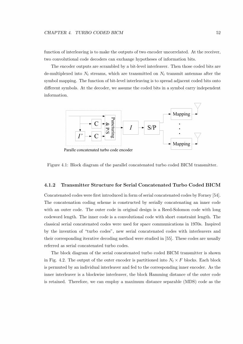
CHAPTER 4. TURBO CODED BICM 52
function of interleaving is to make the outputs of two encoder uncorrelated. At the receiver,
two convolutional code decoders can exchange hypotheses of information bits.
The encoder outputs are scrambled by a bit-level interleaver. Then those coded bits are
de-multiplexed into Nt streams, which are transmitted on Nt transmit antennas after the
symbol mapping. The function of bit-level interleaving is to spread adjacent coded bits onto
different symbols. At the decoder, we assume the coded bits in a symbol carry independent
information.
I’
I
Mapping
Mapping
Paralle concatenated turbo code encoder
Punctu
ring
& P
/S
Figure 4.1: Block diagram of the parallel concatenated turbo coded BICM transmitter.
4.1.2 Transmitter Structure for Serial Concatenated Turbo Coded BICM
Concatenated codes were first introduced in form of serial concatenated codes by Forney [54].
The concatenation coding scheme is constructed by serially concatenating an inner code
with an outer code. The outer code in original design is a Reed-Solomon code with long
codeword length. The inner code is a convolutional code with short constraint length. The
classical serial concatenated codes were used for space communications in 1970s. Inspired
by the invention of “turbo codes”, new serial concatenated codes with interleavers and
their corresponding iterative decoding method were studied in [55]. These codes are usually
referred as serial concatenated turbo codes.
The block diagram of the serial concatenated turbo coded BICM transmitter is shown
in Fig. 4.2. The output of the outer encoder is partitioned into Nt × F blocks. Each block
is permuted by an individual interleaver and fed to the corresponding inner encoder. As the
inner interleaver is a blockwise interleaver, the block Hamming distance of the outer code
is retained. Therefore, we can employ a maximum distance separable (MDS) code as the

CHAPTER 4. TURBO CODED BICM 53
outer code, which enables the system to achieve the Singleton bound in the SISO case.
C_Outer
I’1(1) C_Inner
I’Nt(F) C_Inner
I1(1)
INt(F)
Mapping
Mapping
Serial concatenated turbo code encoder
Figure 4.2: Block diagram of the serial concatenated turbo coded BICM transmitter.
4.1.3 Iterative Detection
The receiver is composed of two parts as shown in Fig. 4.3: a signal processing unit in
the front end followed by a turbo decoder. Both signal processing unit and decoder accept
soft inputs and generate soft outputs. The extrinsic information is exchanged between two
parts in an iterative manner.
Turbo
decoder
Signal
Processing
unit
Figure 4.3: Block diagram of the receiver with iterative detection and decoding.
The structure of turbo decoder is different between parallel concatenated turbo codes
and serial concatenated turbo codes. The details of turbo code decoding algorithm are
elaborated in [53]. In this section, we will focus on the signal processing part.
The goal of the signal processing is to derive soft reliability of each coded bit, which
will be used as inputs of the decoder. From (1.26), the received signal at antenna i can be

CHAPTER 4. TURBO CODED BICM 54
expressed as
yi =
Nt∑
j=1
hi,jxj + ni, (4.1)
where the time index t is dropped for convenience. Nt symbols are transmitted simultane-
ously on Nt transmit antennas
x = [x1, x2, · · · , xNt ]. (4.2)
As each symbol xj consists of M coded bits, those Nt symbols are mapped using a vector
of coded bits of length MNt
c = [c1, c2, · · · , cM , · · · , cNtM ]. (4.3)
The a posteriori log-likelihood ratio (LLR) value for the lth coded bit cl in c is
λ(cl) = logPr[cl = 1|y1, · · · , yNr ]
Pr[cl = 0|y1, · · · , yNt ]
= log
∑
c:cl=1
Pr[y1, · · · , yNr , c]
∑
c:cl=0
Pr[y1, · · · , yNr , c]
= log
∑
c:cl=1
Pr[y1, · · · , yNr |c]Pr(c)∑
c:cl=0
Pr[y1, · · · , yNr |c]Pr(c).
(4.4)
We apply following approximation in above algorithm
log(ea + eb) = max(a, b) + log(1 + e−|a−b|) ≈ max(a, b). (4.5)
At high SNR, the correction term log(1 + e−|a−b|) can be ignored, which leads a small
degradation in performance. In (4.4), the log-sum computation can be simplified by max-
log approximation
log∑
c:cl=1
Pr[y1, · · · , yNr |c]Pr(c) ≈ maxc:cl=1
log Pr[y1, · · · , yNr |c]Pr(c). (4.6)
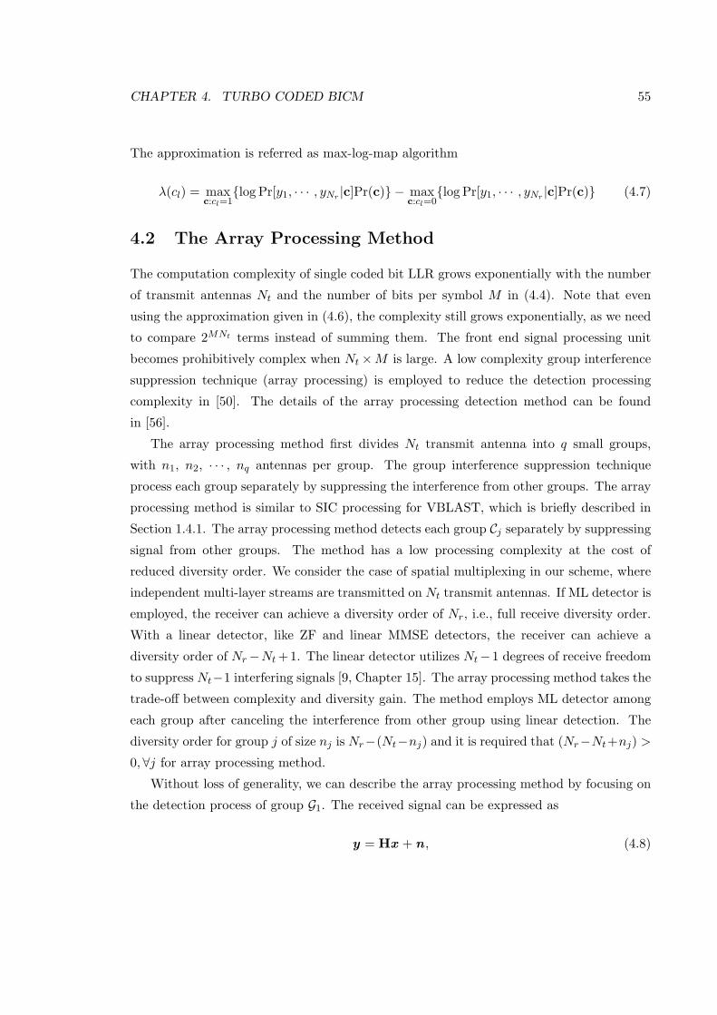
CHAPTER 4. TURBO CODED BICM 55
The approximation is referred as max-log-map algorithm
λ(cl) = maxc:cl=1
log Pr[y1, · · · , yNr |c]Pr(c) − maxc:cl=0
log Pr[y1, · · · , yNr |c]Pr(c) (4.7)
4.2 The Array Processing Method
The computation complexity of single coded bit LLR grows exponentially with the number
of transmit antennas Nt and the number of bits per symbol M in (4.4). Note that even
using the approximation given in (4.6), the complexity still grows exponentially, as we need
to compare 2MNt terms instead of summing them. The front end signal processing unit
becomes prohibitively complex when Nt ×M is large. A low complexity group interference
suppression technique (array processing) is employed to reduce the detection processing
complexity in [50]. The details of the array processing detection method can be found
in [56].
The array processing method first divides Nt transmit antenna into q small groups,
with n1, n2, · · · , nq antennas per group. The group interference suppression technique
process each group separately by suppressing the interference from other groups. The array
processing method is similar to SIC processing for VBLAST, which is briefly described in
Section 1.4.1. The array processing method detects each group Cj separately by suppressing
signal from other groups. The method has a low processing complexity at the cost of
reduced diversity order. We consider the case of spatial multiplexing in our scheme, where
independent multi-layer streams are transmitted on Nt transmit antennas. If ML detector is
employed, the receiver can achieve a diversity order of Nr, i.e., full receive diversity order.
With a linear detector, like ZF and linear MMSE detectors, the receiver can achieve a
diversity order of Nr−Nt+1. The linear detector utilizes Nt−1 degrees of receive freedom
to suppress Nt−1 interfering signals [9, Chapter 15]. The array processing method takes the
trade-off between complexity and diversity gain. The method employs ML detector among
each group after canceling the interference from other group using linear detection. The
diversity order for group j of size nj is Nr−(Nt−nj) and it is required that (Nr−Nt+nj) >
0, ∀j for array processing method.
Without loss of generality, we can describe the array processing method by focusing on
the detection process of group G1. The received signal can be expressed as
y = Hx + n , (4.8)

CHAPTER 4. TURBO CODED BICM 56
where x is the transmitted symbol vector of size Nt, y is the received signal vector of size
Nr and H is channel matrix of dimensions Nr × Nt. The channel matrix can be divided
into two parts
H = [ΩG1 ΛG1 ], (4.9)
where the first part has n1 columns
ΩG1 =
h1,1 h1,2 · · · h1,n1
h2,1 h2,2 · · · h2,n1
......
. . ....
hNr,1 hNr,2 · · · hNr,n1
, (4.10)
and the second part has the Nt − n1 columns
ΛG1 =
h1,n1+1 h1,n1+2 · · · h1,Nt
h2,n1+1 h2,n1+2 · · · h2,Nt
......
. . ....
hNr ,n1+1 hNr,n1+2 · · · hNr,Nt
. (4.11)
To cancel the (Nt − n1) interference signals from the other (q − 1) groups, we construct a
nulling matrix ΘG1 of dimensions (Nr − (Nt − n1))×Nr, where we have 0 = ΘG1ΛG1 . The
nullity of ΛG1 , i.e., the dimension of the NULL space N of ΛG1
dim(N ) = Nr − rank(ΛG1) ≥ Nr −Nt + n1. (4.12)
The (Nr −Nt + n1) rows in ΘG1 are a set of orthonormal vectors (not necessarily unique)
from the NULL space N of ΛG1
v1, v2, · · · , vNr−Nt+n1. (4.13)
There are several numerical methods to compute the NULL space N of the matrix ΛG1 ,
including Gaussian elimination (column or row reduction), QR decomposition and singu-
lar value decomposition (SVD). We choose QR decomposition, which has good numerical

CHAPTER 4. TURBO CODED BICM 57
stability and moderate computation complexity. The matrix ΛG1 can be factorized as
ΛG1 = QG1RG1 = [Q1G1
Q2G1]
[R1
G1
0
], (4.14)
where QG1 is an Nr ×Nr unitary matrix and RG1 of is an Nr × (Nt − n1) upper triangular
matrix. The matrix QG1 consists of two parts, Q1G1
and Q2G1. The first part Q1
G1is composed
of (Nr−Nt+n1) columns, which span the the NULL space N of the matrix ΛG1 . The actual
computation of QR decomposition can be performed by Householder transformation [57,58].
After obtaining the nulling matrix ΘG1 , we multiply both sides of (4.8) by ΘG1
ΘG1y = ΘG1Hx +ΘG1n . (4.15)
The new input-output relation can be simplified as
yG1= HG1xG1 + nG1 , (4.16)
where
yG1= ΘG1y ,
HG1 = ΘG1ΩG1 ,
xG1 = [x1, x2, · · · , xn1 ]T ,
nG1 = ΘG1n .
(4.17)
As QG1 is an Nr × Nr unitary matrix, the process does not enhance noise vector. the In
(4.16), the interference signals from the rest (q − 1) groups are removed by linear nulling
operation. Then we can apply (4.4) to calculate coded bit reliabilities within group G1.
4.3 Sphere Decoder with Max-Log MAP Performance
The array processing method achieves the low demodulation complexity by suppressing
the interference from other groups. The cost of decreased complexity is the performance
degradation due to reduced diversity order. Unlike ZF (inverse channel detector), the
array processing method does not enhance the noise power. The method actually utilizes
receive diversity to cancel interference from other groups. In addition, the group interference
suppression technique was originally designed for system with individual codes per layer.

CHAPTER 4. TURBO CODED BICM 58
Such system benefits from previous successfully decoded layers. The performance of the
group interference suppression technique deteriorates in the case where a single code is used
for all layers of the system. This motivates us to employ sphere decoder [51, 52] to reduce
processing complexity and achieve good performance.
The basic idea of sphere decoding is illustrated in Fig. 4.4. The skewed lattice represents
the distorted signal points. The sphere decoding algorithm will only search signal points
that stay within the sphere of radius r and centered at received signal y . However, it is
difficult to set the value of radius r. If r is too large, the decoding complexity will be still
high, because the algorithm will still considers many points. If r is too small, we may not
include any signal point in the sphere. Another difficulty about sphere decoding is how
to efficiently check which point lies within the sphere. Basically, we need to calculate the
distance from the received signal to signal point
r2 ≥ |y −Hx |2. (4.18)
If we calculate the above distance explicitly for each signal point in the constellation, we
do not gain any complexity advantage of using sphere decoding over maximum-likelihood
(ML) decoding.
r
Figure 4.4: Geometrical interpretation of sphere decoding.
Different versions of sphere decoding algorithm have been proposed in literatures [51,
59, 60]. Almost all of these sphere decoding algorithms are based on QR factorization of
the channel matrix H , which breaks the distance calculation in (4.18) into stages. The
calculation is terminated at the early stage, if the partial distance exceeds the radius r.
The detection algorithm can be implemented as a depth first tree search.

CHAPTER 4. TURBO CODED BICM 59
Recently, a soft-input soft-output single tree search sphere decoder was proposed in [52].
Their algorithm is capable to incorporate a priori information and generate max-log soft
estimation with reduced complexity. Assuming Nr ≥ Nt, the algorithm starts with QR-
decomposition of the channel matrix
H = [Q Q′]
[R
0
]= QR, (4.19)
where [Q Q′] is an Nr × Nr unitary matrix and Q represents its first Nt columns. R is a
Nt ×Nt upper-triangular matrix. After preprocessing, we have the modified input-output
relation
y = QHy = Rx+QHn, (4.20)
where QH denotes the conjugate-transpose of Q and components in QHn are indepen-
dent complex Gaussian random variable of variance N0. Then the max-log LLRs can be
calculated as
λ(cl) = minc:cl=−1
1
N0|y−Rx|2 − log Pr(c)
− minc:cl=1
1
N0|y−Rx|2 − log Pr(c)
.
(4.21)
We defined MAP metric λMAP , which is associated with the MAP solution as
λMAP = minall c
1
N0|y−Rx|2 − log Pr(c)
. (4.22)
And the competitor metric for coded bit cl is defined as
λMAP (cl) = minc:cl=−cMAP
l
1
N0|y−Rx|2 − log Pr(c)
. (4.23)
With above definitions, the log-MAP output can be express as
λ(cl) =
λMAP (cl)− λMAP , cMAP
l = 1
λMAP − λMAP (cl), cMAPl = −1
. (4.24)
The distance
d(c) =1
N0|y−Rx|2 − log Pr(c) (4.25)
in (4.22) and (4.23) can be calculated recursively using the fact thatR is an upper-triangular

CHAPTER 4. TURBO CODED BICM 60
matrix. We define distance increment ei for step-i as
ei =1
N0|yi −
Nt∑
j=i
Ri,jxj |2 − log Pr(ciM+1, · · · c(i+1)M ). (4.26)
The distance d(c) can be calculated with partial distance (PD) di in the following recursion:
• Initialization: dNt+1 = 0;
• Recursive evaluation: di = di+1 + ei;
• End: d(c) = d1.
With above recursive method of evaluating d(c), the detection can be transformed into
a tree traversal problem. An example of sphere decoding tree for BPSK constellation and
Nt = 4 transmit antennas is shown Fig. 4.5.
-1 +1 -1 +1 -1 +1 -1 +1 -1 +1 -1 +1 -1 +1 -1 +1
-1 +1 -1 +1 -1 +1 -1 +1
-1 +1 -1 +1
-1 +1
Root
Lev: 4
Lev: 3
Lev: 2
Lev: 1
e1
e2
e3
e4
d5=0
d4
d3
d2
d1
Figure 4.5: Sphere decoding search tree for BPSK constellation with Nt = 4.
The Tree Pruning Criterion
The sphere decoding method proposed in [52] adopts a technique known as radius reduction
[61]. In this way, the search avoids the problem of choosing a proper radius r. The algorithm
initializes λMAP and λMAP (cl), ∀l to be ∞, which guarantees the MAP solution for every
coded bits. The method updates the radius using d(c) → r2, whenever a valid leaf in the

CHAPTER 4. TURBO CODED BICM 61
tree is reached. The depth-first search will remove a node’s and its children from further
consideration, if current partial distance is already larger than the radius constraint
di ≥ r2. (4.27)
Tree traversal is performed depth-first in sphere decoding. The search starts at the root and
goes deeper in the tree until a leaf is reached or the current node is abandoned according
to the general pruning criterion 4.27. The children of a node are visited in ascending order
of their partial distance.
The tree traversal is confined within the subtree, which can lead to an update of either
λMAP or any counter-hypotheses λMAP (cl). Let us assume the search arrives at a node at
the level-i in the tree search.
1. The counter-hypotheses λMAP (cl) above level-i (towards root):
Denote by cl a bit in the current search branch above level-i. If cl = cMAPl , the counter
hypothesis λMAP (cl) may be get updated by searching the subtree. We denote the
set of counter-hypotheses in this category as A1.
2. The counter-hypotheses λMAP (cl) below level-i: As the node is not expanded yet,
all counter-hypotheses λMAP (cl) below-i may be updated in searching the subtree.
We denote the set of counter-hypotheses in this category as A2.
The partial distance di is compared with the counter-hypotheses in both A1 and A2. We
denote the the union of the two sets as A = A1 ∪A2. The node’s subtree will be pruned if
di > maxλ∈A
λ. (4.28)
According to the discussion above, the tree-pruning criterion ensures that we cannot provide
update to any counter-hypotheses. The set A does not contain the current MAP hypothesis
λMAP , but any counter hypothesis will be larger than λMAP . Therefore, (4.28) is a sufficient
condition for tree-pruning operation.
The decoding complexity of max-log-MAP algorithm can be greatly decreased by tree-
pruning. However, the the complexity of this version of sphere decoding algorithm is not
fixed. We will discuss the factors that affect decoding complexity latter in Section 4.3.
Some examples of complexity results are presented in Section 4.5.

CHAPTER 4. TURBO CODED BICM 62
The list administration
When a valid leaf is reached in the tree traversal, the detector will update the current MAP
hypothesis λMAP and counter-hypotheses λMAP (cl), ∀l ∈ [1, NtM ].
1. d(c) < λMAP : A new MAP hypothesis is found. If the bit cl is changing in the MAP
hypothesis, the counter-hypothesis for cl should also be updated.
• Counter-hypothesis update: λMAP → λMAP (cl) for changing cl in MAP hypoth-
esis cMAP
• MAP hypothesis cMAP update: d(c) → λMAP
2. d(c) ≥ λMAP : In this case, only counter-hypotheses might be updated. For the the
coded bit cl in c, we check whether cl is the same as the bit cMAPl in MAP hypothesis.
If they are different, we will update counter-hypothesis for cl, when d(c) < λMAP (cl).
• Counter-hypothesis update: d(c) → λMAP (cl)
Two conditions are required: cl 6= cMAPl and d(c) < λMAP (cl).
The complexity
The visited nodes are denoted by red dots in Fig. 4.5. The complexity of the sphere decoding
is a function of both the number of the visited nodes and the operations associated with each
node. However, we only consider the expected number of nodes as a measure of decoding
complexity in this research. The total complexity can be reduced by the tightened tree-
pruning criterion, which still generates max-log outputs [52]. The decoding complexity is
significantly reduced with a high SNR. Because many candidates become less probable with
at high SNR and the nodes are pruned at early stage of the tree traversal. We will show
simulation results in the next section.
4.4 K-Best Sphere Decoding with Fixed Complexity
In Section 4.3, we described a soft-input soft-output sphere detector, which achieves max-
log MAP performance. The disadvantage of the detection method is that the complexity of
the processing is not fixed. For practical application, the hardware design needs to satisfy
the worst-case situation. Therefore, it is preferred to have a sphere decoder with fixed
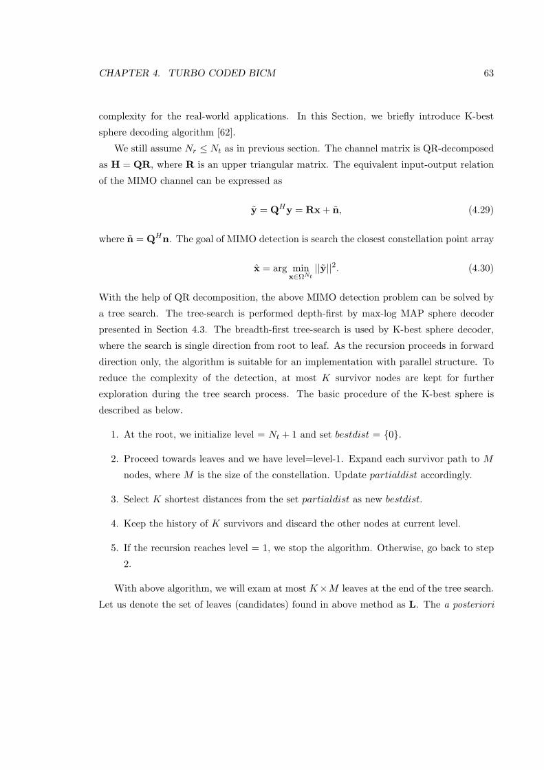
CHAPTER 4. TURBO CODED BICM 63
complexity for the real-world applications. In this Section, we briefly introduce K-best
sphere decoding algorithm [62].
We still assume Nr ≤ Nt as in previous section. The channel matrix is QR-decomposed
as H = QR, where R is an upper triangular matrix. The equivalent input-output relation
of the MIMO channel can be expressed as
y = QHy = Rx+ n, (4.29)
where n = QHn. The goal of MIMO detection is search the closest constellation point array
x = arg minx∈ΩNt
||y||2. (4.30)
With the help of QR decomposition, the above MIMO detection problem can be solved by
a tree search. The tree-search is performed depth-first by max-log MAP sphere decoder
presented in Section 4.3. The breadth-first tree-search is used by K-best sphere decoder,
where the search is single direction from root to leaf. As the recursion proceeds in forward
direction only, the algorithm is suitable for an implementation with parallel structure. To
reduce the complexity of the detection, at most K survivor nodes are kept for further
exploration during the tree search process. The basic procedure of the K-best sphere is
described as below.
1. At the root, we initialize level = Nt + 1 and set bestdist = 0.
2. Proceed towards leaves and we have level=level-1. Expand each survivor path to M
nodes, where M is the size of the constellation. Update partialdist accordingly.
3. Select K shortest distances from the set partialdist as new bestdist.
4. Keep the history of K survivors and discard the other nodes at current level.
5. If the recursion reaches level = 1, we stop the algorithm. Otherwise, go back to step
2.
With above algorithm, we will exam at most K×M leaves at the end of the tree search.
Let us denote the set of leaves (candidates) found in above method as L. The a posteriori

CHAPTER 4. TURBO CODED BICM 64
log-likelihood ratio (LLR) value for the lth coded bit cl in c is calculated over the L
λ(cl) = logPr[cl = 1|y1, · · · , yNr ]
Pr[cl = 0|y1, · · · , yNt ]
= log
∑
c∈L:cl=1
Pr[y1, · · · , yNr , c]
∑
c∈L:cl=0
Pr[y1, · · · , yNr , c]
= log
∑
c∈L:cl=1
Pr[y1, · · · , yNr |c]Pr(c)∑
c∈L:cl=0
Pr[y1, · · · , yNr |c]Pr(c).
(4.31)
In the iterative detection, the candidate list L will be calculated only once at the first
iteration. The a priori information Pr(c) and the a posteriori information λ(cl) will be
updated at each iteration. The details of the K-best algorithm can be found in [62].
4.5 Simulation results
In this section, simulation results for turbo coded BICM schemes in block-fading channels
are presented. We first compare the performance and complexity between sphere decoding
method and array processing method with a large number of antennas. Then, we present
and compare the performance between serial and parallel turbo coded BICM schemes in
block-fading channels.
4.5.1 Performance of sphere decoder
We consider a system with large number of transmit and receive antennas. Sphere decoder
described in Section 4.3 is employed at the signal processing unit to generate estimates
for coded bits, which are used as inputs for the turbo decoder. At the transmitter side,
a parallel concatenated turbo coded BICM scheme is used. The configuration of the par-
allel concatenated turbo coded BICM follows exactly the structure of those in [50], where
two systematic recursive (1, 5/7) convolutional codes are employed and the parity bits are
punctured regularly to get a coding rate of rc = 1/2. A random interleaver is employed
between the parallel turbo encoder and modulator. The codeword length is 1024 bits for
both schemes.
We compare the FER performance of the sphere decoding and array processing method

CHAPTER 4. TURBO CODED BICM 65
(group interference suppression) described in Section 4.2 with 10 rounds of the iterative
detection in Fig. 4.6. Each codeword spans F = 2 independent fading blocks. The turbo
code internal decoding iteration is set to be 1 to reduce the total computation at the receiver.
In group interference suppression, we partition 4 transmit antennas into two group of two
antennas and partition 8 transmit antennas into three group of 3, 3 and 2 antennas. At a
FER of 10−3, we can see that sphere decoder provides a gain of 5dB for the 4 × 4 MIMO
case and a gain of 6dB for the 8×8 MIMO case. The performance loss with array processing
method is caused by reduced diversity with linear processing to null the interference signals
from other groups. The sphere decoding achieves max-log-map performance. However, the
sphere decoding performance curve is not parallel to outage curve, which means it fails
to achieve the full diversity order. The parallel concatenated turbo coded BICM scheme
proposed in [50] does not guarantee achievable diversity order. This observation inspires us
to explore the serial concatenated codes for MIMO block-fading channels, which is actually
designed for SISO block-fading channels.
−10 −8 −6 −4 −2 0 2 4 6 8 1010
−4
10−3
10−2
10−1
100
Eb/No (dB)
FE
R
4x4 MIMO Sphere
4x4 MIMO Array
8x8 MIMO Sphere
8x8 MIMO Array
4x4 MIMO Outage
8x8 MIMO Outage
d = 32 d = 128
Figure 4.6: FER performance comparison between sphere decoding and array processingover a block-fading channel with F = 2.

CHAPTER 4. TURBO CODED BICM 66
It is interesting to perform a complexity comparison between sphere decoding and group
inference suppression. The complexity of sphere decoding is data dependent and the com-
plexity of group interference suppression is fixed. We compute the complexity of sphere
decoding by finding the average number of nodes visited during the tree transversal in Fig.
4.7.
1 2 3 4 5 6 7 8 9 1020
25
30
35
40
45
50
55
60
65
70
Iterations
Av
erag
e n
um
ber
of
nodes
−10db
−5db
−4db
−3db
−2db
0db
−1db
Figure 4.7: Average number of nodes visited during the sphere decoding search in a 4 × 4MIMO block-fading channel with F = 2.
The complexity of sphere decoding decreases when the number of iterations or SNR
increases. For 4×4 MIMO channel and QPSK modulation, there are a total of 340 nodes in
the sphere decoding tree. At a high SNR, we need to search about 25 nodes at the 10th iter-
ation, which are 7% of the total nodes. With a low SNR value, we need to process 65 nodes
at the 10th iteration, which are 19% of the total nodes. For group interference suppression,
we divide 4 transmitter antennas into two groups, with two antennas in each group. For
QPSK modulation, we need to process 42 = 16 sequences in each group. The complexity of
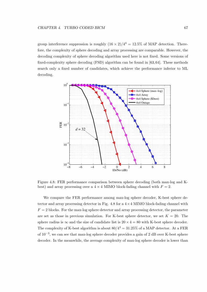
CHAPTER 4. TURBO CODED BICM 67
group interference suppression is roughly (16 × 2)/44 = 12.5% of MAP detection. There-
fore, the complexity of sphere decoding and array processing are comparable. However, the
decoding complexity of sphere decoding algorithm used here is not fixed. Some versions of
fixed-complexity sphere decoding (FSD) algorithm can be found in [63,64]. These methods
search only a fixed number of candidates, which achieve the performance inferior to ML
decoding.
−8 −6 −4 −2 0 2 4 6 810
−4
10−3
10−2
10−1
100
Eb/No (dB)
FE
R
4x4 Sphere (max−log)
4x4 Array
4x4 Sphere (Kbest)
4x4 Outage
d = 32
Figure 4.8: FER performance comparison between sphere decoding (both max-log and K-best) and array processing over a 4× 4 MIMO block-fading channel with F = 2.
We compare the FER performance among max-log sphere decoder, K-best sphere de-
tector and array processing detector in Fig. 4.8 for a 4×4 MIMO block-fading channel with
F = 2 blocks. For the max-log sphere detector and array processing detector, the parameter
are set as those in previous simulation. For K-best sphere detector, we set K = 20. The
sphere radius is ∞ and the size of candidate list is 20× 4 = 80 with K-best sphere decoder.
The complexity of K-best algorithm is about 80/44 = 31.25% of a MAP detector. At a FER
of 10−3, we can see that max-log sphere decoder provides a gain of 2 dB over K-best sphere
decoder. In the meanwhile, the average complexity of max-log sphere decoder is lower than

CHAPTER 4. TURBO CODED BICM 68
K-best sphere decoder in this situation.
−10 −8 −6 −4 −2 0 2 410
−4
10−3
10−2
10−1
100
Eb/No (dB)
FE
R
8x8 Sphere (max−log)
8x8 Array
8x8 Sphere (Kbest)
8x8 Outage
d = 128
Figure 4.9: FER performance comparison between sphere decoding (both max-log and K-best) and array processing over a 8× 8 MIMO block-fading channel with F = 2.
The FER performance comparison of max-log sphere decoder, K-best sphere detector
and array processing detector is show in Fig. 4.9, on a 8 × 8 MIMO block-fading channel
with F = 2 blocks. At a FER of 10−3, max-log sphere decoder offers a gain of 3 dB over
K-best sphere decoder. We still set sphere radius to be ∞ for K-best sphere detector. As
we have more transmit antennas in the system, the value of K increases to 64. The size of
candidate list is 64 × 4 = 256 and the detection complexity of K-best algorithm is about
256/48 = 0.39% of a MAP detector.
4.5.2 Comparison between serial and parallel turbo codes
To make a fair comparison, the serial concatenated turbo codes employ a non-systematic,
non-recursive, 3-memory convolutional code as the outer code and a single memory accu-
mulator as the inner code. Therefore, there are 4 memories in both parallel turbo code
and serial turbo code encoders. The codeword length is 1024 and the number of iterative

CHAPTER 4. TURBO CODED BICM 69
detection is 10 for both schemes. QPSK modulation is used in our simulations.
−5 0 5 10 15 2010
−5
10−4
10−3
10−2
10−1
100
Eb/No (dB)
FE
R
Nr=1 F=4 Parallel
Nr=1 F=4 Serial
Nr=2 F=2 Parallel
Nr=2 F=2 Serial
Nr=1 F=4 Outage
Nr=2 F=2 Outage
d = 8
d = 8
Figure 4.10: FER performance for parallel and serial concatenated turbo coded BICMscheme with Nt = 2 and QPSK modulation.
We compare frame error rate (FER) performance of parallel and serial concatenated
turbo coded BICM in Fig. 4.10. The simulations are carried out in block-fading channel
with F = 2 and F = 4. We use a (11, 15) convolutional code as the outer code for the
Nt = 2, Nr = 2, F = 2 case and a (13, 11) convolutional code for the Nt = 2, Nr = 1, F = 4
case. Both outer codes for the serial concatenated turbo codes are MDS codes for SISO
block fading channel [10]. Our results show that parallel turbo coded BICM outperforms
serial turbo coded BICM in MIMO block-fading channels. The total available diversity
order is 8 for both channel conditions. It can be seen that both schemes fail to achieve full
diversity order, because there are interference signals present in the MIMO transmission.
We apply use spatial multiplexing and send different data streams on different transmit
antennas to achieve the high throughput at the cost of reduced spatial diversity order.
To further illustrate the effect of interference, we compare parallel and serial concate-
nated turbo coded BICM in a simple SISO case with Nt = 1, Nr = 1, F = 2 and a simple

CHAPTER 4. TURBO CODED BICM 70
MIMO case with Nt = 2, Nr = 1, F = 1. Two cases have the same outage limit. A (13, 15)
convolutional code is employed as the outer code for the serial concatenated turbo code.
As shown in Fig. 4.11, the serial concatenated turbo coded BICM achieves the optimal
diversity order of 2 in the SISO case, but parallel concatenated turbo coded BICM fails
to achieve the optimal diversity order. However, both schemes fails to achieve the optimal
diversity order with Nt = 2, where spatial interference is present. The reason is that the
serial concatenated turbo code proposed in [2] is for SISO channel. A direct application of
this scheme to MIMO case will not guarantee the achievable diversity order.
−5 0 5 10 15 20 25 3010
−4
10−3
10−2
10−1
100
Eb/No (dB)
FE
R
Nt=1 Nr=1 F=2 Parallel
Nt=1 Nr=1 F=2 Serial
Nt=2 Nr=1 F=1 Parallel
Nt=2 Nr=1 F=1 Serial
Outage for both cases
d = 2
Figure 4.11: FER performance for parallel and serial concatenated turbo coded BICMscheme in both SISO and MIMO block-fading channels.
In the next chapter, we will explore a MIMO transmission based on modulation diver-
sity techniques for block-fading channels. The method enables spatial multiplexing with
loosing any spatial diversity. The cost of the modulation diversity technique is extra system
structure at the transmitter and increased possessing complexity at the receiver.
CHAPTER 4. TURBO CODED BICM 71
4.6 Conclusions
In this chapter, we studied turbo coded BICM schemes for MIMO block-fading channels.
The research can be viewed as a supplementary work to the parallel concatenated turbo
coded BICM scheme in [50]. A serial concatenated turbo coded BICM scheme is proposed.
Two schemes are compared in terms of performance in MIMO block-fading channels. In
addition, a sphere decoder is used as a practical low-complexity signal processing solution,
when the number of transmit antennas or the size of modulation constellation is large. The
sphere decoder offers better performance compared with the group suppression technique.
The decoding complexity of sphere decoding is comparable to that of group suppression
technique.
Our study also shows that we cannot apply schemes derived for SISO block-fading
channels to MIMO cases directly to achieve full space diversity. The reason is that we need
to deal with interference from different transmit antennas in the MIMO case. In the next
chapter, will show a hybrid scheme based on both error correcting codes and space-time
codes to achieve the full diversity order of the channel.

Chapter 5
Coded MIMO Systems with
Modulation Diversity for
Block-Fading Channels
We propose a new coded multiple-input multiple-output (MIMO) scheme based on modu-
lation diversity technique for block-fading channels. The proposed scheme can achieve both
full spatial multiplexing and full diversity of NtNrF , i.e., the product of the number of
transmit antennas Nt, receive antennas Nr, and fading blocks F . The design concatenates
a channel code with a space-time code. The channel code provides time diversity and coding
gain, whereas the space-time code is employed to achieve space diversity. Since the modula-
tion diversity technique enables full space diversity and full spatial multiplexing at the cost
of increased processing complexity at the receiver, sphere decoding is employed to reduce
the detection complexity. Simulation results are provided to demonstrate the effectiveness
of the proposed schemes in MIMO block-fading channels.
It has been shown that for a coded system over a block-fading channel the maximum
achievable diversity order is upper bounded by the Singleton bound [10]. If a MIMO system
relies on channel coding only to obtain the full diversity order of NtNrF , the maximum
code rate is rc = 1/NtF . Such a low rate is unacceptable in many applications. Space-
time coding techniques can be employed to exploit partial or full space diversity of NtNr.
Space-time block codes based on orthogonal designs are able to achieve full space diversity
with low-complexity receiver at the expense of low rate (no more than 1 symbol per channel
72

CHAPTER 5. CODED ST WITH MODULATION DIVERSITY 73
use) [24]. Layered space-time codes increase transmission rate with reduced diversity [28].
We are interested in space-time codes, which can achieve full space diversity of NtNr with
full spatial multiplexing (Nt symbols per channel use), such as the threaded algebraic space-
time codes discussed in [65] and the recently proposed MIMO systems with real value
constellation rotations [66]. These full-diversity and full-rate space-time code designs are
based on multidimensional constellation expansion (rotation), i.e., modulation diversity
techniques proposed in [67], which spreads constellation points over the time and space
domains. At the receiver, a joint maximum-likelihood (ML) detector over time and space
domains is required to achieve modulation diversity.
We propose a coded MIMO scheme, which can achieve the full diversity order of NtNrF
and transmit at full rate over block-fading channels. The design concatenates a channel code
with a space-time code. The channel code provides time diversity and coding gain, while the
space-time code allows for space diversity. At the receiver, a near optimal iterative belief
propagation (BP) detection algorithm is used and the extrinsic information is exchanged
between the space-time signal detector and the channel decoder. Furthermore, an efficient
soft-input soft-output sphere decoder is employed as signal detector to reduce the detection
complexity [52].
5.1 Space-Time Coding Based on Modulation Diversity
Modulation diversity technique was originally proposed for fully-interleaved SISO fading
channels [67]. The basic idea is to spread constellation points over the time domain by ro-
tation operation, such that each original constellation point experiences independent fading
coefficients. At the receiver a ML detector is equipped to exploit the modulation diversity.
The modulation diversity technique can be employed for space diversity orders in MIMO
systems. The diagonal algebraic space-time (DAST) block codes based on rotated constel-
lations and Hadamard transform can achieve full space diversity order and a throughput of
1 symbol per channel use [68]. The threaded algebraic space-time (TAST) codes achieves
both full diversity order and full rate (Nt symbols per channel use) [65]. The TAST scheme
obtains full rate by using the space-time threading architecture proposed in [69]. The full
diversity order is achieved by transmitting a scaled DAST code in each thread. The TAST
coding scheme is also refereed as universal space-time coding (USTC). Both DAST scheme
and TAST encode coded bits onto complex-valued QAM symbols directly. We follow a

CHAPTER 5. CODED ST WITH MODULATION DIVERSITY 74
transmission design based on real-valued rotation threads for MIMO system [66], which
adopt a design similar to TAST and also achieves both full diversity and full rate.
Modulation diversity techniques and space-time codes based on real-valued rotations are
introduced briefly here. Let z = [z1, z2, · · · , zNt ]T denotes an Nt-dimensional vector with
real elements, where zi ∈ ±1,±3, · · · ,±(2M2 −1) is a point in a PAM constellation of size
2M2 . The mapping scheme transmits M bits per two dimensions, which is equivalent to a
QAM constellation of 2M points. The rotated vector u is obtained by multiplying vector z
by a real orthogonal rotation matrix RNt of size Nt as
u = RNtz. (5.1)
The rotation process spreads PAM points in z over all elements in u. So that each point
will go through different fading effects. Let us denote the real PAM constellation set by
ZNt and the rotated constellation set by UNt . We have
UNt = u|u = RNtz, z ∈ ZNt. (5.2)
Let ua and ub be two vectors from the rotated constellation set UNt . And ua,j and ub,j
are jth component in vector ua and ua, respectively. The following two code design criteria
are employed to guarantee diversity order and good coding gain for the SISO fading channel
case [67].
• The modulation diversity order: The minimum number of distinct components be-
tween any two rotated vectors in UNt .
• The product distance:
dp,min = minua,ub∈UNt
Nt∏
j=1
|∆uj|, (5.3)
where ∆uj= ua,j − ub,j 6= 0.
The optimized rotation matrices RNt , which enable the system to achieve full diversity
and good minimum product distance can be found in [67]. For example, the optimal real
rotation matrix with Nt = 2 is
R2 =
[0.5257 −0.8507
0.8507 0.5257
]. (5.4)
CHAPTER 5. CODED ST WITH MODULATION DIVERSITY 75
For Nt = 3, the optimal rotation matrix is given by
R3 =
α β γ
β γ α
−γ −α −β
, (5.5)
where
α =1 + ω
1 + ω + ω2, β = ωα and γ =
−ω
1 + ωα with ω = 2 cos(6π/7). (5.6)
The space-time code design to minimize the maximum pairwise error probability (PEP)
with ML detection follows the famous rank criterion and determinant criterion proposed
for MIMO channel in [24] .
• Full rank criterion: To ensure that the resulting space-time code achieves full space
diversity with ML decoding, any difference codeword matrix (xa − xb) has to be full
rank Nt (assuming Nr ≥ Nt), where xa and xb are from space-time codeword set XNt .
• Determinant criterion: Let D , xa − xb and Γ = DDH . The Λj is the jth non-zero
eigenvalue of Γ, with k = 1, 2, 3, · · · , Nt. The minimum determinant (5.7) over any
pair of codewords should be maximized.
dp,min = minxa,xb∈XNt
Nt∏
j=1
Λxj, (5.7)
For layered MIMO transmission, the data are de-multiplexed into streams at the trans-
mitter side and each of them is referred to as a layer [28]. A thread is defined as a layer
with full spatial and temporal span [70]. Each thread is active during all transmission in-
tervals during the time, which requires Nt to be no less than the total number of threads
(with complex elements). The thread switches to a different transmission antenna at each
transmission interval and each thread uses Nt transmission antennas equally often. The ad-
vantage of space-time threading is that each thread will experience all available diversities
in both time and space domain.
In [66], a threaded space-time code of dimension Nt×Nt is constructed by 2Nt u threads
as shown in (5.8). The resulting layered space-time code transmits MNt bits per channel
use, which has the same spectral efficiency as full spatial multiplexing MIMO system with
a 2M -QAM constellation. A scaling number is introduced for each thread to guarantee full

CHAPTER 5. CODED ST WITH MODULATION DIVERSITY 76
x =
x1,1 x1,2 · · · x1,Nt
x2,1 x2,2 · · · x2,Nt
......
. . ....
xNt,1 xNt,2 · · · xNt,Nt
=
u1,1 + juNt+1,1 u2Nt,2 + juNt,2 · · · uNt+2,Nt + ju2,Nt
u2,1 + juNt+2,1 u1,2 + juNt+1,2 · · · uNt+3,Nt + ju3,Nt
......
. . ....
uNt,1 + ju2Nt,1 uNt−1,2 + ju2Nt−1,2 · · · u1,Nt + juNt+1,Nt
(5.8)
rank [65]. The thread ui is constructed by
ui = φiRNtzi, (5.9)
where φi’s are referred as Diophantine numbers
φ1 = 1, φ2 = φ1/Nt , · · · , φNt = φ(Nt−1)/Nt,
and φi = φi−Nt , for i ≥ Nt +1. It has been shown that φ = ejπ/6 for Nt = 2 and φ = ejπ/12
for Nt = 3 yield optimal coding gain and ensure the full rank property [65]. An example of
threaded layering scheme is illustrated in Fig.5.1. The numbers are used to denote threads
and there are a total of 6 real threads in the example for Nt = 3.
1 + j4
1 + j4
1 + j4
2 + j5
2 + j5
5 + j26 + j3
3 + j6
6 + j3
Figure 5.1: The threaded layers in space-time code scheme with Nt = 3.
The modulation diversity achieves the full diversity order at the cost of increasing pro-
cessing complexity at the receiver side, as it actually encapsulate information about all
bits in the original PAM vector in every single rotated constellation point. In order to
achieve maximum diversity order, ML detection at the receiver is required whose complex-
ity increases exponentially with the constellation size index M and square of the number
of transmission antennas N2t . Therefore, decoding a system with more than 4 transmission

CHAPTER 5. CODED ST WITH MODULATION DIVERSITY 77
antennas using any mapping scheme would be impractical with original ML decoding al-
gorithm. Low complexity ML detector can be implemented in the form of sphere decoder,
which was discussed in Section 4.3.
5.2 System Model of Coded MIMO System Based on Mod-
ulation Diversity
The proposed coded MIMO system consists of two parts: an outer channel code and an
inner space-time code. The two parts are serially concatenated by a bit-level blockwise
interleaver, which scrambles the the coded bits for each fading block separately. Therefore,
the distance property is reserved after blockwise interleaving. The outer channel code is
selected to be a maximum distance separable (MDS) code for SISO block-fading channels,
which provides time diversity. The inner space-time code is responsible for space diversity.
A more general design is possible as discussed in [71]. A low rate channel code can be used
to collect partial space diversity and alleviate the processing burden of space-time code
detector. However, a more complicated design is needed to enable the outer channel code
to exploit space diversity. We only consider the system splitting time and space diversity
collection duties to two parts.
5.2.1 Transmitter Structure
The block diagram of the transmitter structure is shown in Fig. 5.2.
MDS
Channel
Code
Encoder
Blockwise
Bit-level
Interleaver
S-T Code
Encoder1. PAM Modulation
2. Rotation
3. Space-time Mapping
Figure 5.2: Transmitter structure of the coded MIMO system.
We choose serial concatenated turbo codes proposed in [2] as the channel code, which
consists of an outer MSD non-systematic convolutional code and an inner repeat accumulate
(RA) code. The output of the outer encoder is partitioned into F blocks, one for each fading

CHAPTER 5. CODED ST WITH MODULATION DIVERSITY 78
block in the time domain. A blockwise interleaver is inserted between the channel encoder
and space-time code encoder, so the blockwise Hamming distance of the outer channel code
is retained after interleaving. We use the space-time code presented in Section 5.1 as the
inner code to exploit space diversity. The space-time unit encodes MN2t coded bits into a
space-time code x with dimensions Nt ×Nt as shown in (5.8) at each operation.
5.2.2 Receiver with Iterative Detection
Turbo
decoder
Signal
Processing
unit
Figure 5.3: Block diagram of the receiver with iterative detection and decoding.
The receiver is composed of two parts as shown in Fig. 5.3; a signal processing unit
in the front end followed by a channel code decoder. Both parts accept soft inputs and
generate soft outputs. The extrinsic information is exchanged between two parts in an
iterative manner.
As each space-time symbol x consists of N2t M coded bits, the signal processing unit has
to perform a joint ML detection on those bits. Let c of length N2t M be the coded bits
c = [c1, c2, · · · , cM , · · · , cN2t M
]. (5.10)
Assuming a maximum a posteriori (MAP) detector is employed, the a posteriori log-
likelihood ratio (LLR) value for the lth coded bit cl in c is
λ(cl) = logPr[cl = 1|y]Pr[cl = 0|y] = log
∑
c:cl=1
Pr[y|c]Pr(c)∑
c:cl=0
Pr[y|c]Pr(c). (5.11)
Thanks to bit-level interleaver, we can assume that the a priori probabilities Pr(cl) from

CHAPTER 5. CODED ST WITH MODULATION DIVERSITY 79
channel decoder are statistically independent. The extrinsic information ξ(cl) fed back to
channel decoder is
ξ(cl) = log
∑
c:cl=1
Pr[y|c]
∏
m 6=l
Pr(cl)
∑
c:cl=0
Pr[y|c]
∏
m 6=l
Pr(cl)
. (5.12)
In (5.11) and (5.12), we have
Pr [y|c] = K exp
(−‖y −Hx‖2F
N0
), (5.13)
where x is the space-time code mapped from c, K is a constant and ‖ · ‖F is Frobenius
norm.
The soft-input soft-output channel code decoding algorithm can be found in [2], which
also includes an iterative process of extrinsic information exchange between outer convolu-
tional code decoder and inner RA code decoder. To reduce the complexity of total decoding
complexity, the inner iteration number is set to be 1.
The detection complexity of a single coded bit grows exponentially with N2t M in (5.11).
The log-sum computation in (5.11) can be simplified by max-log approximation without
much performance loss
log∑
c:cl=1
Pr[y|c]Pr(c) ≈ maxc:cl=1
log Pr[y|c]Pr(c). (5.14)
However, the search candidates complexity of (5.14) still grows exponentially with N2t M .
Compared with a V-BLAST system in [28] with the same settings, the number of candidate
space-time codes x increases from 2NtM to 2Nt2M . The increased detection complexity with
diversity modulation is the cost of getting diversity gain. A soft-input soft-output sphere
decoder [51,52] can be employed to reduce processing complexity without performance loss.
In order to apply the existing sphere decoding algorithms to the proposed MIMO system,
some transforms are needed. We start with the case with two transmit antennas. From

CHAPTER 5. CODED ST WITH MODULATION DIVERSITY 80
(5.8), the space-time code can be expressed as
x = [x1,x2] =
[u1,1 + ju3,1 u4,2 + ju2,2
u2,1 + ju4,1 u1,2 + ju3,2
].
Similarly, we represent channel matrix, noise matrix and received signal matrix in (1.26)
in using column vectors as H = [h1,h2], n = [n1,n2] and y = [y1,y2]. The input-output
relation of the channel can be rewritten as
[y1
y2
]=
[H 0
0 H
][x1
x2
]+
[n1
n2
]. (5.15)
Considering the structure of space-time code given in (5.15), we can further transform the
term
[H 0
0 H
][x1
x2
]in (5.15) to
[h1 0 h2 0 h3 0 h4 0
0 h2 0 h3 0 h4 0 h1
]
u1
u2
u3
u4
,
where h3 = jh1 and h4 = jh2. The real thread ui is obtained by ui = φiR2zi in (5.9).
Therefore, we can take PAM vector zi as inputs and rewrite (5.15) as
[y1
y2
]= H′
z1
z2
z3
z4
+
[n1
n2
], (5.16)
where H′ is the new equivalent channel matrix of dimensions 2Nr × 8
H′ =
[h1 0 h2 0 h3 0 h4 0
0 h2 0 h3 0 h4 0 h1
]
φ1R2 0 0 0
0 φ2R2 0 0
0 0 φ1R2 0
0 0 0 φ2R2
.

CHAPTER 5. CODED ST WITH MODULATION DIVERSITY 81
The above transformations can be easily generalized to system with any number of transmit
antennas Nt. The general equivalent channel input-output relation can be expressed as
y1
y2
...
yNt
= H′
z1
z2...
z2Nt
+
n1
n2
...
nNt
, (5.17)
where H′ is the general equivalent channel matrix with dimensions NtNr × 2N2t
Most existing sphere decoding algorithms like [51, 52] can be directly applied to (5.17).
For MIMO block-fading channels, the equivalent channel matrix H′ only needs to be com-
puted once per fading block.
5.3 Simulation Results
In this section, we present simulation results of the proposed coded MIMO systems over
block-fading channels.
Let us first consider a 2 × 1 MIMO quasi-static Rayleigh fading (F = 1) channel. We
intend to show that full space diversity can be achieved by the proposed coded scheme
with this channel. The size of PAM constellation is two, i.e., BPSK modulation. The
system throughput is 4 bits per channel use. The outer channel code is a blockwise con-
catenated convolutional code (BCCC) proposed in [2], which consists of a 1/2-rate (5, 7)
non-systematic non-recursive convolutional code (MDS code for F = 2) and a memory-1
RA code. The codeword length is 1024 for all of our simulation results in this chapter. The
BCCC code is designed to achieve maximum diversity over SISO block-fading channels.
After channel coding, the coded bits are interleaved and then encoded by the space-time
code using Equation (5.8). For comparison, we consider a MIMO system using a BCCC
channel code to exploit space diversity, where the coded bits of the BCCC encoder are first
partitioned blockwise, then QPSK modulated and sent on two transmit antennas. We also
plot the performance of the BCCC code over a SISO block-fading channel with F = 2,
which has the same intrinsic channel diversity as a 2×1 quasi-static fading MIMO channel.
We compare the FER performance of the proposed MIMO space-time scheme based on
rotated constellation (Rotated ST) with BCCC code in Fig. 5.4. The simulation results

CHAPTER 5. CODED ST WITH MODULATION DIVERSITY 82
−5 0 5 10 15 20 25 3010
−4
10−3
10−2
10−1
100
Eb/No (dB)
FE
R
Nt=1 F=2 BCCC
Nt=2 F=1 BCCC
Nt=2 F=1 Rotated ST
Outage for both
d = 2
Figure 5.4: FER performance of the coded MIMO system over a 2× 1 MIMO quasi-staticfading channel.

CHAPTER 5. CODED ST WITH MODULATION DIVERSITY 83
are obtained with a MAP detector as show in (5.11) and 10 rounds of iterative detection-
decoding. We can see that the proposed coded MIMO scheme achieves full diversity of 2
with the help of space-time code based on modulation diversity technique. The BCCC code
can achieve full diversity in the SISO case, but fails to achieve full diversity in the MIMO
case. The reason is that BCCC can be used for space diversity based on the assumption
that interferences can be fully removed at the detector, which is an ideal situation. To
achieve space diversity with ML detection, the rank criterion must be satisfied [24]. We
also note that the system throughput of the SISO case is 2 bits per channel use, which is half
of the MIMO case. Spacial multiplexing gain and space diversity gain are two attractive
achievements with MIMO systems.
−5 0 5 10 15 2010
−4
10−3
10−2
10−1
100
Eb/No (dB)
FE
R
Nt=2 Nr=1 Rotated ST
Nt=2 Nr=2 Rotated ST
Nt=3 Nr=3 Rotated ST
d = 4
d = 8
d = 18
Figure 5.5: FER performance of the coded MIMO system over MIMO block-fading channelswith F = 2 fading blocks.
In the next step, we test the proposed system in MIMO block-fading channels with
F = 2 fading blocks. The channel code settings are the same as those in the previous case.
The space-time code needs to be adjusted according to the number of transmit antennas.
We simulate 3 MIMO settings: 2× 1, 2× 2 and 3× 3. In the first MIMO setting, a MAP

CHAPTER 5. CODED ST WITH MODULATION DIVERSITY 84
signal detector is used. In the second and third settings, a soft-input soft-output sphere
detector is used. A system throughput of 4 bits per channel use is achieved for Nt = 2
and 6 bits per channel use for Nt = 3. The number of iterations is 15 for all cases. Both
simulated FER performance and their corresponding outage limits with Gaussian inputs
(by curves using the same line styles without marker) are drawn in Fig. 5.5. We can see
that all three FER curves are parallel to their corresponding outage limits, which means all
of them achieve full time and space diversity.
2 4 6 8 10 12 14
20
30
40
50
60
70
Iterations
Aver
age
num
ber
of
nodes
8dB
1dB
0dB
2dB
−2dB
−10dB
Figure 5.6: Average number of nodes visited during the sphere decoding search in a 2 × 2MIMO block-fading channel with F = 2 fading blocks.
For the simulation with sphere decoder, we have adopted the soft-input soft-output single
tree search algorithm proposed in [52], which is capable to incorporate a priori information
and generate max-log estimation. The signal detection can be transformed into a tree search
problem and a tree pruning criterion is provided to avoid searching the entire tree. The
average number of visited nodes during the detection process can be used as a measure
of decoding complexity. Assuming Nr ≥ Nt, there are a total of∑2N2
t
i=1 2i = 510 nodes

CHAPTER 5. CODED ST WITH MODULATION DIVERSITY 85
with Nt = 2 and PAM constellation of size two. We show average number of nodes visited
for 2 × 2 MIMO block-fading channel with F = 2 in Fig. 5.6. We can see that the signal
processing cost has been greatly reduced by using sphere decoder. The detection complexity
of sphere decoder is a function of the SNR and the number of iterations. The detection
complexity decreases, as the SNR or the number of iteration increases. At a SNR of 8dB
and 15 iterations, an average of 21 nodes need to be processed, which are just 4.1% of the
total nodes. We also note that at low SNR, the detection complexity is almost unchanged
with different number of iterations, which means the feedbacks from channel decoder are
unreliable and do not provide much help in signal separation.
−4 −2 0 2 4 6 810
−4
10−3
10−2
10−1
100
Eb/No (dB)
FE
R
Serially Turbo−coded BICM
Space−Time modulation diversity
Outage bound
d = 8
Figure 5.7: Comparison of FER performance between the coded MIMO system and theserically Turbo-coded BICM scheme withNt = 2, Nr = 2, over MIMO block-fading channelsof F = 2 fading blocks.
We already show the diversity advantage of proposed coded space-time scheme based on
modulation diversity over the BCCC scheme in Fig.5.4, where the total available diversity
order is 2. Now we consider a 2 × 2 MIMO system over a block-fading channel of F = 2
blocks. In this situation, the total available diversity order is 8. We compare the proposed
CHAPTER 5. CODED ST WITH MODULATION DIVERSITY 86
scheme with the corresponding scheme without modulation diversity. In both schemes, we
use BCCC codes, where a 1/2-rate (5, 7) non-systematic non-recursive convolutional code
is used as the outer code and a memory-1 RA code is used as inner code. As we discussed
in Chapter 4, the serially concatenated BCCC is originally designed for SISO block-fading
channels, which is not guaranteed to achieve full diversity order in MIMO channels. From
Fig. 5.7, we observe the scheme with modulation diversity has only marginal advantage in
performance over the scheme without modulation diversity when total available diversity
order is 8. The reason is that when there are more available diversity (≥ 8), the system
without modulation diversity has high probability to obtain a high diversity order and its
performance is close to the system with full diversity order. The systems designed for
block-fading channels show superior performance by achieving full diversity order for the
situation, where the total available diversity is limited (≤ 4).
5.4 Conclusions
In this chapter, we proposed a coded MIMO scheme for block-fading channels. The pro-
posed scheme consists of a channel code and a space-time code. The channel code is selected
to be a MDS code designed for SISO block-fading channels and the function of the channel
is to provide time diversity. The space-time code is designed based on modulation diversity
technique, which allows full spatial multiplexing MIMO transmission and achieves full space
diversity at the same time. The drawback of modulation diversity is the increased complex-
ity at the detector. We also show how to apply a sphere decoder to the proposed system to
reduce the signal processing complexity. Simulation results have verified the effectiveness
of our designs over MIMO block-fading channels. Here, we use channel coding to achieve
time diversity and space-time coding for space diversity. We would like to mention that a
general design is also possible, in which the processing complexity can be traded for code
rate.

Chapter 6
An Efficient Decoding Algorithm
for Concatenated
RS-Convolutional Codes
6.1 Introduction
The code design criterion for error correcting codes over block-fading channels is to find
block-wise maximum distance separable (MDS) codes with large coding gain. The Reed-
Solomon (RS) codes are an important class of MDS codes, which were invented by Reed and
Solomon in 1960 [72]. The RS codes cannot be directly applied to block-fading channels,
because we consider fading channel with only a few fading blocks (F ≤ 8) and the codeword
length of RS codes is usually longer than that. For block-fading channels with number of
fading blocks F = 4, 6 and 8, lengthening (adding information symbols) and shortening
(removing information symbols) of RS codes are proposed in [10]. However, in this chapter
we focus on standard RS codes design and their decoding. The results can be applied to
lengthened and shortened RS codes for block-fading channels.
Concatenated schemes using Reed-Solomon codes as the outer code and convolutional
codes as the inner code have been widely used for deep space communications as well as
digital video broadcasting systems [73]. Convolutional codes can sweep channel noise, while
RS codes can combat burst errors which are caused by the the decoding process of convo-
lutional codes when a Viterbi decoder is employed. Using this method, the concatenated
87

CHAPTER 6. RS-CONVOLUTIONAL CODES 88
coding schemes can achieve high coding gains.
The concatenated Reed-solomon/Convolutional (RS/Conv) coding scheme has been
around for a long time, but using iterative decoding schemes based on turbo principle
for decoding these codes is relatively new. The main reason is that the soft input soft
output (SISO) decoding algorithms for RS code are usually complicated, especially when
codeword length is long. In 1994, Pyndiah et al. developed a simple and effective SISO
decoder for RS codes based on the Chase algorithm. Pyndiah’s algorithm has been used
for turbo decoding of both product [74] and serial concatenated codes [75].
In this chapter, we improve the decoding algorithm for the concatenated RS/Convo
scheme investigated in [75] by adopting Kaneko’s algorithm for RS decoding [76]. This idea
is inspired by [77], in which the authors discussed how to reduce decoding complexity of
turbo product codes. The proposed algorithm reduces the computational complexity by em-
ploying the stopping criteria during the Chase decoding process. While conventional Chase
algorithm generates constant number of codeword candidates, we expect to examine fewer
number of codeword candidates using Kaneko’s stopping criteria. The major advantage of
the proposed algorithm is lower computational complexity without sacrificing performance
loss.
6.2 The Reed-Solomon Codes
The RS code is probably the most widely used traditional error control scheme in the
coding society. After their invention in 1960s, the RS codes were employed in numerous
applications in digital media and systems due to their excellent performance in combating
random and burst symbol errors. In this section, we provide a brief introduction to RS
codes. More detailed description of RS codes can be found in [38, 78].
The RS codes have been employed by various digital storage schemes for error protection.
They are adopted in compact disc (CD) standard in the form of cross-interleaved Reed-
Solomon (CIRS) coding, which is used to recover the information loss caused by scratches
on the disc surface [79]. The RS codes are also found with various machine-readable bar-
code systems including popular quick response (QR) code [80]. With the error correction
provide by RS codes, the machine can still decode a barcode with damage up to certain
level. Other than consumer electronics, the RS codes are used in communication system as
well, including digital video broadcasting and deep space communications.

CHAPTER 6. RS-CONVOLUTIONAL CODES 89
Let’s consider an (n, k, d) RS code constructed over Galois field GF (q), where n is the
codeword symbol length, k is the information symbol length and d is the minimum symbol
Hamming distance. There are a total of q = 2m elements in Galois field GF (2m) and each
element can be represented using m bits.
The standard RS code has a codeword length of n = 2m − 1. The minimum Hamming
distance is d = n−k+1, as RS codes are MDS codes. The code can detect up to d−1 = n−k
erroneous symbols and correct up to t = ⌊(n − k)/2⌋ erroneous symbols. By design, one
can select information length to be k = 2m − 1− 2t and the minimum distance of the code
is d = 2t+ 1. The code can correct any single burst error of length m(t− 1) + 1 bits.
6.2.1 The RS Code Encoding
RS codes are cyclic codes, which can be generated using a generator polynomial of degree
(n− k) over GF (2m).
G(x) = xn−k + gn−k−1xn−k−1 + · · ·+ g1x+ g0, (6.1)
where gi, i ∈ [0, n− k − 1] is an element from GF (2m). The encoding of RS codes can be
done in either a systematic way or a non-systematic way.
• For non-systematic encoding, we simply multiply the information symbol polynomial
U(x) by the generator polynomial G(x)
C(x) = U(x)G(x), (6.2)
where U(x) = uk1xk−1 + · · ·u1x+ u0, with gi ∈ GF (2m), 0 ≤ i < k − 1.
• For systematic encoding, the codeword is obtained by
Csys(x) = xn−kU(x)− [xn−kU(x) mod G(x)]. (6.3)
It is easy to verify Csys(x) is a valid codeword, as G(x) divides Csys(x). The first k
symbols in Csys(x) are raw information symbols and the remaining n−k symbols are
parity-check symbols.
The generator polynomials of RS codes are the minimal polynomials of αi, b ≤ i ≤ b+2t−1,
where α is the primitive element of Galois field GF (q) and b is an integer; usually b = 0

CHAPTER 6. RS-CONVOLUTIONAL CODES 90
or b = 1. The primitive element α of GF (q) is a generator of the field, where q is the
smallest value such that αq−1 = 1. The minimal polynomial of β ∈ GF (q) is defined as
the a polynomial of the lowest degree over GF (q) that has β as its root. Therefore, the
generator of RS codes can be expressed as
G(x) =b+2t−1∏
i=b
(x− αi). (6.4)
Thanks to the above special structure, there exist computationally efficient decoding algo-
rithms for RS codes.
6.2.2 Decoding of RS Codes
RS codes are non-binary Bose-Chaudhuri-Hocquenghem (BCH) codes and therefore any
decoding algorithm for BCH codes can be applied to decode RS codes [38, 78]. Here we
briefly describe the well-known Berlekamp-Massey algorithm, which is used to find the error
locations [81]. For non-binary code, the error value can be any non-zero element in GF (q).
Compared with binary BCH codes, the additional stage required for decoding RS codes is
to find the error magnitudes, which can be done by using Forney algorithm. This step is
not required by binary BCH codes, because we can simply flip the bit at each error location.
Let us denote the received vector using R(x) = C(x) + E(x), where C(x) is the trans-
mitted codeword and E(x) is the error polynomial. The error polynomial E(x) can be
expressed as
E(x) = ej1xj1 + ej2x
j2 + · · ·+ ejvxjv , (6.5)
where eji is error magnitude and ji is the error location for 1 < i ≤ v. By design, the
generator polynomial has αi, b ≤ i ≤ b+2t− 1, as its roots. Therefore, we have C(αi) = 0
for b ≤ i ≤ b + 2t − 1. The syndromes are calculated by evaluating R(x) at x = αi with
b ≤ i ≤ b+ 2t− 1. The resulting syndrome polynomials are expressed as
S1 = R(αb) = ej1αbj1 + ej2α
bj2 + · · ·+ ejvαbjv
S2 = R(α(b+1)) = ej1α(b+1)j1 + ej2α
(b+1)j2 + · · ·+ ejvα(b+1)jv
......
S2t = R(α(b+2t−1)) = ej1α(b+2t−1)j1 + ej2α
(b+2t−1)j2 + · · ·+ ejvα(b+2t−1)jv
. (6.6)
If syndromes are all zeros, the codeword is considered to be received correctly. Otherwise,

CHAPTER 6. RS-CONVOLUTIONAL CODES 91
we need to find the error locations and error values by investigating the syndromes. The
error locator polynomial is defined as
σ(x) =v∏
k=1
(1− αjkx) = 1 + σ1x1 + · · ·+ σv−1x
v−1 + σvxv. (6.7)
Finding the zeros of σ(x) are equivalent to obtaining the error locations. We have σ(α−jk) =
0, where jk is one of the error locations. The σ(α−jk) can be expanded as
0 = 1 + σ1α−jk + · · ·+ σv−1α
−(v−1)jk + σvα−v(jk). (6.8)
In the next step, we relate syndromes and error locations without error values.
1. Multiplying both sides of (6.8) by ejkαbjk+vjk , we obtain
0 = ejkαbjk+vjk + σ1ejkα
bjk+(v−1)jk + · · ·+ σvejkαbjk . (6.9)
2. Summing (6.9) from k = 1 to v, we have
0 =v∑
k=1
ejkαbjk+vjk +
v∑
k=1
σ1ejkαbjk+(v−1)jk + · · ·+
v∑
k=1
σvejkαbjk . (6.10)
3. From (6.6), we can express the syndrome Sv+1 as
Sv+1 =v∑
k=1
ejkαbjk+vjk for 0 ≤ v ≤ 2t− 1. (6.11)
We get following relation between error location polynomial coefficients and syndromes by
substituting (6.11) into (6.9)
0 = Sv+1 + σ1Sv + · · ·+ σvS1. (6.12)
If we multiply both sides of (6.8) by ejkαbjk+(v+1)jk in step 1 of above process, we obtain
0 = Sv+2 + σ1Sv+1 + · · ·+ σvS2. (6.13)

CHAPTER 6. RS-CONVOLUTIONAL CODES 92
By repeating the process, we get a set of equations (key equations)
S1 S2 · · · Sv
S2 S3 · · · Sv+1
......
...
Sv Sv+1 · · · S2v−1
σv
σv−1
...
σ1
=
−Sv+1
−Sv+1
...
−Sv+v
. (6.14)
The the equations can be efficiently solved using the Berlekamp-Massey algorithm, which
finds an error locator polynomial (6.7) of minimal degree. The Berlekamp-Massey algorithm
uses an iterative procedure. The detailed description of the algorithm and examples can be
found in [78].
At the step-i, we already have an error locator polynomial σi(x) of degree li
σi(x) = 1 + σi1x
1 + · · ·+ σilixli , (6.15)
which satisfies the following set of equations
li∑
j=0
Sk−jσij = 0, Sk−j ∈ S1, S2, · · · , Si. (6.16)
The discrepancy at the step-i is calculated as
di = Si+1 + σi1Si + · · ·+ σi
liSi−li+1. (6.17)
• If di = 0, we do not need to update the error locator polynomial.Therefore, we get
σ(i+1)(x) = σ(i)(x) and li+1 = li.
• If di 6= 0, we need to compensate the discrepancy. Let σ(m)(x) be the intermediate
solution and (m− lm) is maximal. We update the error locator polynomial as
σ(i+1)(x) = σ(i)(x) + did−1m xi−mσ(m)(x)
li+1 = maxli, lm + i−m. (6.18)

CHAPTER 6. RS-CONVOLUTIONAL CODES 93
The Berlekamp-Massey algorithm starts with
σ(−1)(x) = 1, l−1 = 0, d−1 = 1
σ(0)(x) = 0, l0 = 0, d−1 = S1
. (6.19)
And the process updates error locator polynomial iteratively until i ≥ li+1+t−1 or i = 2t−1.
After obtaining error locator polynomial coefficients σk, we need to find error locations
αjk , which are roots of (6.7). The error locations can be found by Chien search [82], which
simply evaluates (6.7) with each non-zero element β = αi ∈ GF (q). If σ(αi) = 0, we will
accept −i as a valid error location.
The last step of decoding RS codes is to find errors values in (6.5), which is achieved by
Forney algorithm. For the details of Forney algorithm, one can read [38, 78]. The partial
syndrome polynomial is defined as
S(x) , 1 + S1x+ S2x2 + · · ·+ S2tx
2t. (6.20)
And the error evaluator polynomial is defined as
Λ(x) = σ(x)S(x) mod x2t+1. (6.21)
The error value ejl is calculated as
ejl =
(αjl)2−b
Λ(α−jl
)
σ′ (α−jl), (6.22)
where σ′(x) is the derivative of σ(x) with respect to x. With the error values, we can recover
the original codeword using C(x) = R(x)−E(x).
The decoding 4 steps of RS codes are summarized in Table 6.1.
Table 6.1: The decoding procedure for RS codes.
Step 1 compute the syndromes Sj using (6.6)
Step 2 obtain error locator polynomial σ(x) of (6.7) : Berlekamp-Massey algorithm
Step 3 find the error locations: Chien search
Step 4 calculate error values: Forney algorithm
In the next section, an introduction on RS/Conv concatenated coding scheme and the

CHAPTER 6. RS-CONVOLUTIONAL CODES 94
related iterative decoding algorithm used in [75] is presented.
6.3 The RS-Convolutional Concatenated Coding Scheme
Concatenated coding was first proposed by Forney in 1966 [54] in form of RS/Conv serially
concatenated coding scheme. The most famous concatenated coding scheme is probably the
turbo code, which was invented as parallel concatenated convolutional codes in 1993 [53].
In this section, we provide an introduction to the RS/Conv concatenated coding scheme
and an iterative decoding algorithm for it.
The block diagram of the RS/Conv concatenated coding scheme is shown in Fig. 6.1. At
the transmitter side, the RS and the convolutional encoder are connected by an interleaver.
The interleaving scheme has a depth of I, which means that I RS codewords are group
together as the inputs to the encoder of convolutional codes. The interleaving is done at
the bit level. At the receiver side, standard iterative turbo decoding is performed. The
extrinsic information is exchanged between the two decoders. The convolutional decoder
employs the BCJR algorithm and the RS decoder employs Pyndiah’s SISO algorithm [74,75].
RS
Encoder
Convlutional
Encoder
RS
Decoder
DIConvlutional
Decoder
I
I
Channel
Figure 6.1: The block diagram RS/Conv concatenated coding scheme.
The Pyndiah’s algorithm is a soft-input soft-output based on the Chase decoding algo-
rithm [83]. The Chase decoding algorithm is a soft-input hard-output candidate-generating
algorithm. In Chase algorithm, the a certain number of least reliable bits in received vector
Y are inverted to generate a set of test patterns Ym. Those test patterns are fed into a
hard-input hard-output decoder to obtain corrected patterns Xm, i.e., codeword candidates.
The decoded codeword is selected as the codeword candidate with the least soft distance to

CHAPTER 6. RS-CONVOLUTIONAL CODES 95
received vector Y.
Let D be the hard decision codeword, found by the Chase algorithm, which has the
least distance to the received vector Y among all candidates. For a bit dj in D, the soft
reliability is calculated as
rj =Mmin(−dj) −Mmin(dj)
4dj
=|Y−C|2 − |Y−D|2
4dj , (6.23)
where C is the competing codeword which is at the minimum distance from Y among all
candidates with cj = −dj . If at this step we cannot find C, rj is assigned a precalculated
value β(k) ∈ [0, 1], which depends on the number of iteration k. Because the BCJR decoder
uses log-likelihood ratio (LLR) values, the information provided by the RS decoder should
be converted to LLR values which for an AWGN channel is given by
rLLRj = 2× rj/σ2, (6.24)
where σ2 is the variance of the noise. Note that rj is the soft output of the decoder, we
need to subtract the a priori information from rj to generate the extrinsic information. It
is possible that we cannot find the codeword D is our search. If this happens, we simply set
the extrinsic information generated by the RS decoder to be zero. To increase the reliability
during the first iterations, a precalculated scaling parameter γ(k) ∈ [0, 1] for the extrinsic
information is also introduced.
6.4 A Low Complexity Decoding Algorithm
The proposed algorithm is a modified version of Pyndiah’s soft output algorithm for linear
block codes. We add Kaneko’s stopping criterion during the candidate generation process.
Once we find the most likely codeword, the algebraic decoding is halted to reduce the delay
and complexity.
Let us consider a RS code with codeword length n, information length k, and minimum
distance d = n− k + 1, denoted as a (n, k, d) code. The received vector is represented as
Y = y0,y1, · · · ,yn−1, (6.25)
CHAPTER 6. RS-CONVOLUTIONAL CODES 96
where each element consists of q components
yi = yi,0, yi,1, · · · , yi,q−1. (6.26)
For q-ary RS codes, there exist a total of 2q possible symbols. The reliability that yi is
equal to a certain symbol j is calculated as
θi,j = lnp(yi|j)∑l 6=j p(yi|l)
, l ∈ 0, 1, · · · , 2q − 1. (6.27)
Let θ1sti , θ2ndi denote the largest and the second largest components in
θi = θi,0, θi,1, · · · , θi,2q−1. (6.28)
The hard decision sequence YH of Y is obtained by
yHi,j =
0, yi,j ≤ 0, i = 0, 1, · · · , n− 1
1, yi,j > 0, j = 0, 1, · · · , q − 1.(6.29)
LetX be a legitimate codeword in the codeword table. SX denotes the set of positions where
X and YH are equal and ScX is the complement of SX. The likelihood metric L(Y,X) is
calculated as
L(Y,X) =∑
i
θi,xi=∑
i
θi,yHi−∑
i∈ScX
(θi,yH
i− θi,xi
). (6.30)
Since we know Y, the above metric only depends on
l(Y,X) =∑
i∈ScX
(θi,yH
i− θi,xi
)=∑
i∈ScX
(θ1sti − θi,xi
). (6.31)
After receiving Y, we first rearrange its elements in ascending order
θ1stSY(0) − θ2ndSY(0) ≤ θ1stSY(1) − θ2ndSY(1) ≤ · · ·≤ θ1stSY(n−1) − θ2ndSY(n−1).
(6.32)
The basic idea of Kaneko’s algorithm is to search for the codeword X which satisfies the

CHAPTER 6. RS-CONVOLUTIONAL CODES 97
following relation
l(Y,X) <
d−m0−1∑
i=0
(θ1stSY(i) − θ2ndSY(i)), (6.33)
where m0 = ||ScX0
|| is the size of set ScX0
and X0 is the algebraic decoder output when YH
is the input. It can be proved that the codeword satisfying the inequality (6.33) is the most
likely codeword [76]. If we do not find X0, we can use m = ||ScX|| instead of m0 in (6.33).
We test each legitimate codeword we have found during the decoding process using this
inequality. Once the most likely codeword is found, the algebraic decoding is halted and we
start computing the soft outputs using Pyndiah’s soft output algorithm.
Kaneko’s algorithm performs true maximum-likelihood-decoding (MLD) if we do not
limit the number of generated candidate codewords. However, we set a maximum number
of test error patterns in our decoding process as in the Chase algorithm because when the
signal-to-noise ratio (SNR) is low, we need to generate a large set of candidates. In this
situation, finding the most likely codeword takes a long time. It should also be noted that
inequality (6.33) is a sufficient , and not a necessary, condition that X is the ML codeword.
We may miss the most likely codeword and continue to test all possible error patterns. In
this situation, we decode unnecessary error patterns.
The proposed algorithm includes three steps.
1) Generate error patterns.
2) Perform algebraic decoding using each error pattern and test the decoder output
according to (6.33).
The test tells whether the most likely codeword is found. If the most likely codeword
is found or maximum number of tests is reached, continue to step 3); Otherwise, we
go back to step 2) to decode the next error pattern.
3) Calculate soft outputs using Pyndiah’s soft output algorithm.
If the maximum number of tests is reached, the system will perform exactly as the Chase
algorithm does. Otherwise, we will find the most likely codeword in the process and save
processing time. In the next section, we will demonstrate that there is no performance loss
although we generate fewer candidates in the proposed algorithm.
The error patterns are generated using natural binary coding (NBC) in our work. An
example of 8 error patterns is listed in Table 6.2. The bits are sorted by their reliabilities
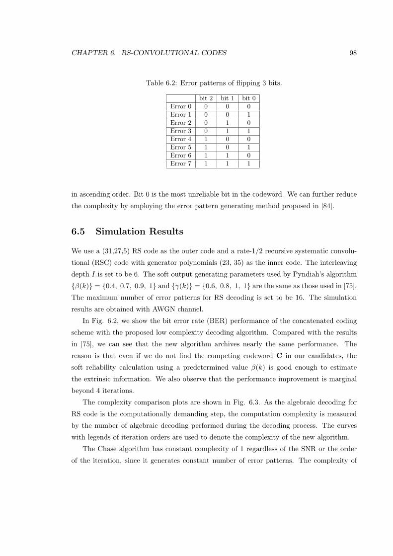
CHAPTER 6. RS-CONVOLUTIONAL CODES 98
Table 6.2: Error patterns of flipping 3 bits.
bit 2 bit 1 bit 0Error 0 0 0 0Error 1 0 0 1Error 2 0 1 0Error 3 0 1 1Error 4 1 0 0Error 5 1 0 1Error 6 1 1 0Error 7 1 1 1
in ascending order. Bit 0 is the most unreliable bit in the codeword. We can further reduce
the complexity by employing the error pattern generating method proposed in [84].
6.5 Simulation Results
We use a (31,27,5) RS code as the outer code and a rate-1/2 recursive systematic convolu-
tional (RSC) code with generator polynomials (23, 35) as the inner code. The interleaving
depth I is set to be 6. The soft output generating parameters used by Pyndiah’s algorithm
β(k) = 0.4, 0.7, 0.9, 1 and γ(k) = 0.6, 0.8, 1, 1 are the same as those used in [75].
The maximum number of error patterns for RS decoding is set to be 16. The simulation
results are obtained with AWGN channel.
In Fig. 6.2, we show the bit error rate (BER) performance of the concatenated coding
scheme with the proposed low complexity decoding algorithm. Compared with the results
in [75], we can see that the new algorithm archives nearly the same performance. The
reason is that even if we do not find the competing codeword C in our candidates, the
soft reliability calculation using a predetermined value β(k) is good enough to estimate
the extrinsic information. We also observe that the performance improvement is marginal
beyond 4 iterations.
The complexity comparison plots are shown in Fig. 6.3. As the algebraic decoding for
RS code is the computationally demanding step, the computation complexity is measured
by the number of algebraic decoding performed during the decoding process. The curves
with legends of iteration orders are used to denote the complexity of the new algorithm.
The Chase algorithm has constant complexity of 1 regardless of the SNR or the order
of the iteration, since it generates constant number of error patterns. The complexity of

CHAPTER 6. RS-CONVOLUTIONAL CODES 99
0 0.5 1 1.5 2 2.5 310
−6
10−5
10−4
10−3
10−2
10−1
100
Eb/No (dB)
BE
R RS/Conv 1st iterationRS/Conv 2nd iterationRS/Conv 3rd iterationRS/Conv 4th iteration
Figure 6.2: BER performance of the concatenated RS/Conv coding system.
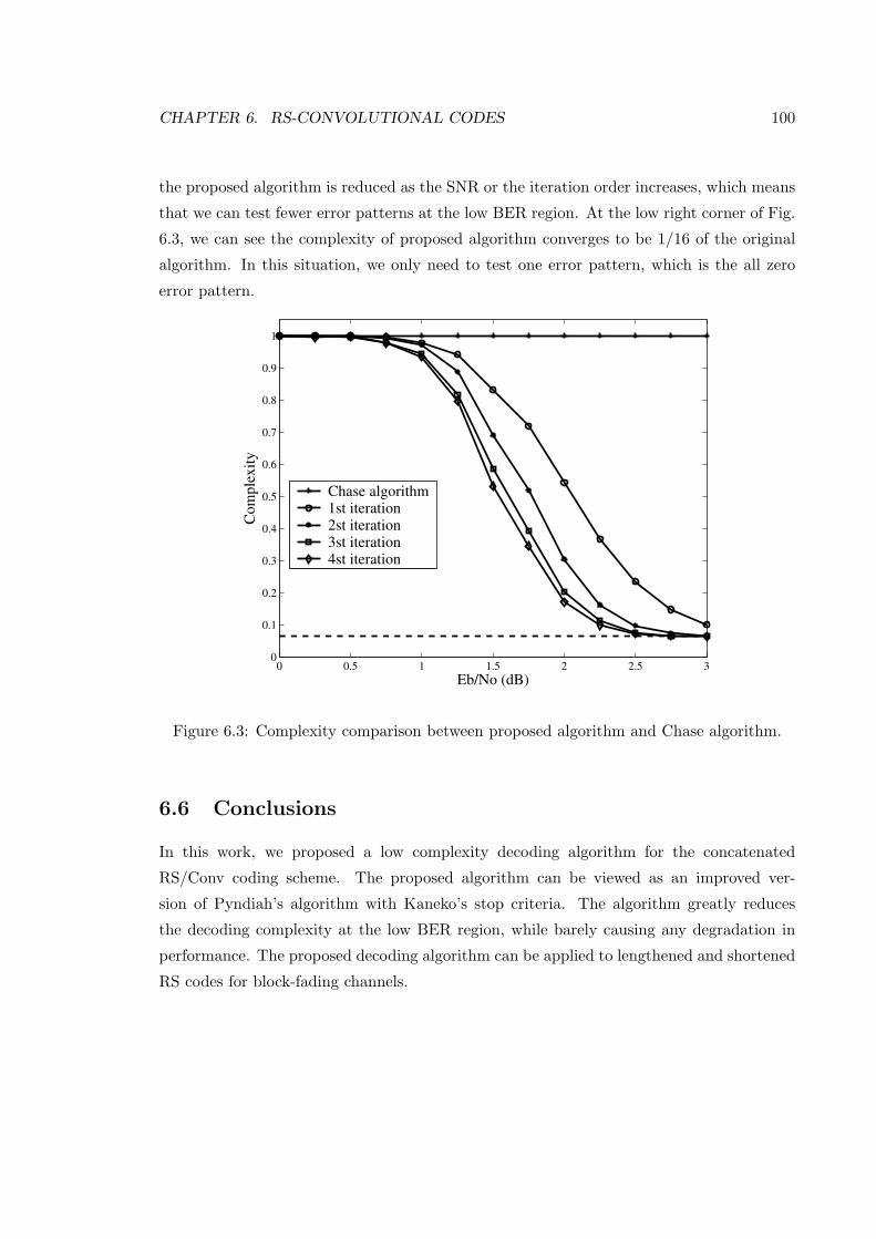
CHAPTER 6. RS-CONVOLUTIONAL CODES 100
the proposed algorithm is reduced as the SNR or the iteration order increases, which means
that we can test fewer error patterns at the low BER region. At the low right corner of Fig.
6.3, we can see the complexity of proposed algorithm converges to be 1/16 of the original
algorithm. In this situation, we only need to test one error pattern, which is the all zero
error pattern.
0 0.5 1 1.5 2 2.5 30
0.1
0.2
0.3
0.4
0.5
0.6
0.7
0.8
0.9
1
Eb/No (dB)
Co
mp
lex
ity
Chase algorithm1st iteration2st iteration3st iteration4st iteration
Figure 6.3: Complexity comparison between proposed algorithm and Chase algorithm.
6.6 Conclusions
In this work, we proposed a low complexity decoding algorithm for the concatenated
RS/Conv coding scheme. The proposed algorithm can be viewed as an improved ver-
sion of Pyndiah’s algorithm with Kaneko’s stop criteria. The algorithm greatly reduces
the decoding complexity at the low BER region, while barely causing any degradation in
performance. The proposed decoding algorithm can be applied to lengthened and shortened
RS codes for block-fading channels.

Chapter 7
Concluding remarks and future
work
7.1 Concluding remarks
The focus of this dissertation is code design for block-fading channels. We first explored code
design criteria for block-fading channels. Two main factors on performance of codes over
block-fading channels are diversity order and coding gain. The Shannon capacity of block-
fading channel is zero; therefore, we employed the outage limit as the ultimate PER lower
bound for any communication systems over block-fading channels. In the first part of the
research, the focus was on code design for SISO block-fading channels. In the second part
of the research, the transmission schemes for MIMO block-fading channels were presented.
We proposed a BC-BICM scheme for block-fading channels. The proposed scheme
is a simplified version of BCC-BICM scheme. The optimal diversity order is achieved by
employing a blockwise MDS outer code. In addition, the coding gain can be improved either
by choosing a carefully designed signal labeling scheme for the BICM with iterative decoding
or by using convolutional codes with longer constraint lengths. Compared with BCC-BICM
scheme, these coding schemes have smaller delays in both encoding and decoding processes.
Simulation results show that the optimized BC-BICM scheme offers similar performance as
the BCC-BICM scheme in block-fading channels but with a simpler system architecture.
We also presented QC-LDPC codes for block-fading channels. A construction method
for designing QC-LDPC codes was presented. With careful design, the proposed QC-LDPC
codes exhibit the same good performance as their corresponding random root-LDPC codes
101
CHAPTER 7. CONCLUSION AND FUTURE WORK 102
with iterative belief-propagation decoding. Moreover, the structure of the proposed QC-
LDPC codes makes them suitable for efficient encoding.
Majority of modern wireless communication systems are equipped with multiple anten-
nas. The two main purposes of using MIMO transmission is to improve the robustness of the
communication by introducing space diversity and to increase transmission rate by spatial
multiplexing. Since the diversity order is limited by channel intrinsic diversity order, i.e.,
the number of fading blocks in the block-fading channel, we consider employing multiple
antennas to provide additional diversity. We investigated turbo coded BICM schemes for
MIMO block-fading channels. Both serial and parallel concatenated turbo codes were con-
sidered and their performance was compared. A sphere decoder was employed to achieve
good performance with reduced computational complexity when the size of the constellation
or the number of transmit antenna is large.
The turbo BICM scheme, however, cannot provide full diversity order. The interference
due to using multiple transmission antennas prevents serial concatenated turbo codes to
achieve the full diversity order in MIMO situation. We proposed a new coded MIMO
scheme based on modulation diversity technique for block-fading channels. The proposed
scheme can achieve both full spatial multiplexing and full diversity of NtNrF , i.e., the
product of the number of transmit antennas Nt, receive antennas Nr and fading blocks
F . The design concatenates a channel code with a space-time code. The channel code
is responsible for providing time diversity and the space-time code is employed to achieve
space diversity. Since the modulation diversity technique enables full space diversity and full
spatial multiplexing at the cost of increased processing complexity at the receiver, sphere
decoding is employed to reduce detection complexity.
The RS codes are well-known MDS codes and they can be modified for block-fading
channels. An efficient decoding algorithm was proposed for concatenated coding schemes
that use a RS code as the outer code and a convolutional code as the inner code. We
compared the proposed decoding algorithm with Pyndiah’s algorithm in terms of both
computational complexity and performance. The proposed decoding algorithm reduces the
decoding complexity by adopting Kaneko’s decoding algorithm without suffering a perfor-
mance loss.
CHAPTER 7. CONCLUSION AND FUTURE WORK 103
7.2 Future work
In our work, we investigated code design for the case, where channel state information
is available only at the receiver side. For MIMO system, precoding and transmitter side
beam-forming techniques can be employed to improve system performance, if channel state
information is known at the transmitter side. The channel information at the transmitter
side is a valid assumption for some modern communication architectures. For example, in
the LTE system with time division duplexing (TDD) where up-link and down-link share
the same frequency channel, the channel information at the transmitter can be obtained
through feedback from the receiver.
Also, we modeled the fading coefficients on each block as independent Rayleigh dis-
tributed random variables. The performance will be degraded, if the fading coefficients on
different blocks are correlated. It is interesting to investigate the performance loss in this
situation.
Bibliography
[1] T. S. Rappaport, Wireless Communications: Principles and Practice, 2nd ed. Engle-
wood Cliffs, NJ: Prentice-Hall, 2002.
[2] A. Fabregas and G. Caire, “Coded modulation in the block-fading channel: Coding
theorems and code construction,” IEEE Trans. Inf. Theory, vol. 52, no. 1, pp. 91–114,
Jan. 2006.
[3] E. Dahlman, S. Parkvall, J. Skold, and P. Beming, 3G Evolution: HSPA and LTE for
Mobile Broadband, 2nd ed. Academic Press, 2008.
[4] S. Sesia, I. Toufik, and M. Baker, LTE: The UMTS Long Term Evolution – From
Theory to Practice. Chichester, UK: J. Wiley & Sons, 2009.
[5] IEEE Std 802.16-2009 Standard for Local and metropolitan area networks Part 16: Air
Interface for Broadband Wireless Access Systems, IEEE Computer Society and IEEE
Microwave Theory and Techniques Society, New York, USA, May 2009.
[6] A. Nosratinia, T. E. Hunter, and A. Hedayat, “Cooperative communication in wireless
networks,” IEEE Communications Magazine, vol. 42, no. 10, pp. 74–80, Oct. 2004.
[7] R. McEliece and W. E. Stark, “Channels with block interference,” IEEE Trans. Inf.
Theory, vol. IT-30, no. 1, pp. 44–53, Jan. 1984.
[8] G. Kaplan and S. Shamai, “Error probabilities for the blockfading gaussian channel,”
Arch. Elektronik Ubertragungstech., vol. 49, no. 4, pp. 192–250, Jul. 1984.
[9] J. Proakis and M. Salehi, Digital Communications, 5th ed. New York: McGraw-Hill,
2007.
104

BIBLIOGRAPHY 105
[10] R. Knopp and P. Humblet, “On coding for block fading channels,” IEEE Trans. Inf.
Theory, vol. 46, no. 5, pp. 1643–1646, Jul. 1999.
[11] E. Malkamaki and H. Leib, “Coded diversity on block-fading channels,” IEEE Trans.
Inf. Theory, vol. 45, no. 5, pp. 1643–1646, Jul. 1999.
[12] A. Fabregas and G. Caire, “Turbo-like codes for the block-fading channel,” in Proc.
IEEE 2004 Int. Symp. Information Theory, Chicago, IL, USA, 2004.
[13] A. Fabregas, “Concatenated codes for block-fading channels,” Ph.D. dissertation,
EPFL, Lausanne, Switzerland, 2004.
[14] E. Biglieri, J. Proakis, and S. Shamai, “Fading channels: Information-theoretic and
communications aspects,” IEEE Trans. Inf. Theory, vol. 44, no. 6, pp. 2619–2692,
Oct. 1998.
[15] E. Malkamaki and H. Leib, “Evaluating the performance of convolutional codes over
block fading channels,” IEEE Trans. Inf. Theory, vol. 45, no. 5, pp. 1643–1646, Jul.
1999.
[16] M. Chiani, A. Conti, and V. Tralli, “Further results on convolutional code search for
block-fading channels,” IEEE Trans. Inf. Theory, vol. 50, no. 6, pp. 1312–1318, Jun.
2004.
[17] J. Boutros, E. Strinati, and A. Fabregas, “Turbo code design for block fading chan-
nels,” in Proc. Allerton Conference on Communication, Control and Computing (42th
Allerton), Monticello, Illinois, Sep. 2004.
[18] G. Kraidy, J. Boutros, and A. Fabregas, “Irregular turbo codes in block fading chan-
nels,” in Proc. International Symposium on Information Theory (ISIT), Austin, Texas,
U.S.A., 2010.
[19] J. Boutros, A. Fabregas, E. Biglieri, and G. Zemor, “Low density parity check codes
for nonergodic block-fading channels,” IEEE Trans. Inf. Theory, vol. 56, no. 9, pp.
4286–4300, Sep. 2010.
[20] I. E. Telatar, “Capacity of multi-antenna gaussian channels,” European Transactions
on Telecommunications, vol. 10, pp. 585–595, Nov. 1999.

BIBLIOGRAPHY 106
[21] A. Goldsmith, S. A. Jafar, N. Jindal, and S. Vishwanath, “Capacity limits of MIMO
channels,” IEEE J. SELECT. AREAS COMMUN, vol. 21, no. 5, pp. 684–702, Jun.
2003.
[22] T. M. Cover and J. A. Thomas, Elements of information theory. New York, NY, USA:
Wiley-Interscience, 1991.
[23] D. Tse and P. Viswanath, Fundamentals of wireless communication. New York, NY,
USA: Cambridge University Press, 2005.
[24] V. Tarokh, N. Seshadri, and A. Calderbank, “Space-time codes for high-data-rate
wireless communication: Performance criterion and code construction,” IEEE Trans.
Inf. Theory, vol. 44, pp. 744–765, Mar. 1998.
[25] S. M. Alamouti, “A simple transmit diversity technique for wireless communications,”
IEEE Journal on Selected Areas in Communications, vol. 44, no. 2, pp. 1451–1458,
Oct. 1998.
[26] A. Goldsmith, Wireless Communications. New York, NY, USA: Cambridge University
Press, 2005.
[27] E. Telatar, “Capacity of multi-antenna gaussian channels,” AT&T-Bell Labs Internal
Technical Memo, Jun. 1995.
[28] G. J. Foschini, “Layered space-time architecture for wireless communication in a fading
environment when using multiple antennas,” IEEE Trans. Inf. Theory, vol. 1, no. 2,
pp. 41–59, Oct. 1996.
[29] X. Wang and H. V. Poor, Wireless Communication Systems: Advanced Techniques for
Signal Reception. Upper Saddle River, NJ, USA: Prentice Hall, 2003.
[30] P. Patel and J. Holtzman, “Analysis of a simple successive interference cancellation
scheme in a DS/CDMA system,” IEEE J Sel Areas Commun, vol. 12, no. 5, pp. 796–
807, 1994.
[31] D. Divsalar, M. K. Simon, and D. Raphaeli, “Improved parallel interference cancella-
tion for CDMA,” IEEE Trans. Commun, vol. 46, pp. 258–268, 1998.

BIBLIOGRAPHY 107
[32] M. Costa, “Writing on dirty paper,” IEEE Transactions on Information Theory,
vol. 29, no. 3, pp. 439–441, May 1983.
[33] H. Weingarten, Y. Steinberg, and S. Shamai, “The capacity region of the gaussian
multiple-input multiple-output broadcast channel,” IEEE Transactions on Information
Theory, vol. 52, no. 9, pp. 3936–3964, Sep. 2006.
[34] D. Gesbert, M. Kountouris, R. W. Heath, C. byoung Chae, and T. Salzer, “From single
user to multiuser communications: Shifting the MIMO paradigm,” vol. 24, no. 5, pp.
36–46, Sep. 2007.
[35] IEEE Std 802.11n-2009 Standard for Information technology Telecommunications and
information exchange between systems Local and metropolitan area networks Specific
requirements Part 11: Wireless LAN Media Access Control (MAC) and Physical Layer
(PHY) Specifications, IEEE Computer Society, New York, USA, Oct. 2009.
[36] X. Li, A. Chindapol, and A. Ritcey, “Bit-interleaved coded modulation with iterative
decoding and 8PSK signaling,” IEEE Trans. Commun., vol. 50, pp. 1250–1257, Aug.
2002.
[37] J. Tan and G. Stuber, “Analysis and design of symbol mappers for iteratively decoded
BICM,” IEEE Trans. Wireless Commun., vol. 4, pp. 662–672, Mar. 2005.
[38] L. Shu and C. Daniel, Error Control Coding, 2nd ed. Upper Saddle River, NJ, USA:
Prentice-Hall, Inc., 2004.
[39] L. Bahl, J. Cocke, F. Jelinek, and J. Raviv, “Optimal decoding of linear codes for
minimizing symbol error rate,” IEEE Trans. Inf. Theory, vol. IT-20, pp. 284–287,
Mar. 1974.
[40] A. Chindapol and J. A. Ritcey, “Design, analysis, and performance evaluation for
BICM-ID with square QAM constellations in rayleigh fading channels,” IEEE Journal
on Selected Areas in Communications, vol. 19, pp. 944–957, 2001.
[41] Y. Li and M. Salehi, “A new bc-bicm scheme for block-fading channels,” in Proc.
Conference on Information Sciences and Systems (CISS2008), Princeton, NJ, Mar.
2008.

BIBLIOGRAPHY 108
[42] Z. Li, L. Chen, L. Zeng, S. Lin, and W. H. Fong, “Efficient encoding of quasi-cyclic low-
density parity-check codes,” IEEE. Trans. Commun., vol. 53, no. 11, pp. 1973–1973,
Jan. 2005.
[43] R. G. Gallager, Low Density Parity Check Codes. Cambridge, Massachusetts: M.I.T.
Press, 1963.
[44] D. J. MacKay and R. M. Neal, “Near shannon limit performance of low density parity
check codes,” Electronics Letters, vol. 32, pp. 1645–1646, 1996.
[45] T. J. Richardson and R. L. Urbanke, “The capacity of low-density parity-check codes
under message-passing decoding,” IEEE Trans. Inf. Theory, vol. 47, pp. 599–618, Feb.
2001.
[46] S. Chung, G. D. Forney, T. J. Richardson, and R. Urbanke, “On the design of low-
density parity-check codes within 0.0045 db of the shannon limit,” IEEE Communica-
tions Letters, vol. 5, pp. 58–60, Feb. 2001.
[47] R. M. Tanner, “A recursive approach to low complexity codes,” IEEE Trans. Inf.
Theory, vol. 27, no. 5, pp. 533–547, Sep. 1981.
[48] M. Fossorier, “Quasi-cyclic low density parity check codes from circulant permutation
matrices,” IEEE Trans. Inf. Theory, vol. 50, no. 8, pp. 1788–1793, Aug. 2004.
[49] S. Srinivasa and A. Weathers, “An efficient on-the-fly encoding algorithm for binary
and finite field LDPC codes,” IEEE Trans. Commun. Lett., vol. 13, pp. 853–855, Nov.
2009.
[50] A. Stefanov and T. Duman, “Turbo-coded modulation for systems with transmit and
receive antenna diversity over block fading channels: System model, decoding ap-
proaches, and practical considerations,” IEEE J. Select. Areas Commun., vol. 19, pp.
958–968, May 2001.
[51] B. Hochwald and S. Brink, “Achieving near-capacity on a multipleantenna channel,”
IEEE Trans. Commun., vol. 51, pp. 389–399, Mar. 2003.
[52] C. Studer and H. Bolcskei, “Soft-input soft-output single tree-search sphere decoding,”
IEEE Trans. Inf. Theory, vol. 56, pp. 4827–4842, Oct. 2010.
BIBLIOGRAPHY 109
[53] C. Berrou, A. Glavieux, and P. Thitimajshima, “Near shannon limit error-correcting
coding and decoding,” in Proc. IEEE International Conference on Communications,
Geneva, Switzerland, 1993.
[54] D. G. F. Jr., “Concatenated codes,” Cambridge, MA, Tech. Rep., 1966.
[55] S. Benedetto, D. Divsalar, G. Montorsi, and F. Pollara, “Serial concatenation of in-
terleaved codes: Performance analysis, design, and iterative decoding,” IEEE Trans.
Inform. Theory, vol. 44, pp. 909–926, 1998.
[56] V. Tarokh, A. Naguib, N. Seshadri, and A. R. Calderbank, “Combined array processing
and space-time coding,” IEEE Trans. Inf. Theor., vol. 45, no. 4, pp. 1121–1128, May
1999.
[57] K. L. Chung and W. M. Yan, “The complex householder transform,” IEEE Transac-
tions on Signal Processing, vol. 45, no. 9, pp. 2374–2376, Sep. 1997.
[58] W. H. Press, W. T. Vetterling, S. A. Teukolsky, and B. P. Flannery, Numerical Recipes
in C++: the art of scientific computing, 2nd ed. New York, NY, USA: Cambridge
University Press, 2002.
[59] B. Hassibi and H. Vikalo, “On the sphere-decoding algorithm. I. Expected complexity,”
IEEE Trans. Sig. Proc., vol. 53, no. 8, pp. 2806–2818, Aug. 2005.
[60] H. Vikalo and B. Hassibi, “On the sphere-decoding algorithm. II. Generalizations,
second-order statistics, and applications to communications,” IEEE Trans. Sig. Proc.,
vol. 53, no. 8, pp. 2819–2834, Aug. 2005.
[61] E. Agrell, T. Eriksson, A. Vardy, and K. Zeger, “Closest point search in lattices,” IEEE
TRANS. INFORM. THEORY, vol. 48, pp. 2201–2214, Aug. 2000.
[62] Z. Guo and P. Nilsson, “Algorithm and implementation of the k-best sphere decoding
for mimo detection,” IEEE J.Sel. A. Commun., vol. 24, no. 3, pp. 491–503, Mar. 2006.
[63] L. G. Barbero and J. S. Thompson, “Extending a fixed-complexity sphere decoder
to obtain likelihood information for Turbo-MIMO systems,” IEEE Transactions on
Vehicular Technology, vol. 57, pp. 2804–2814, Sep. 2008.

BIBLIOGRAPHY 110
[64] L. Barbero and J. Thompson, “Fixing the complexity of the sphere decoder for MIMO
detection,” IEEE Transactions on Wireless Communications, vol. 7, pp. 2131–2142,
Jun. 2008.
[65] H. E. Gamal and M. O. Damen, “Universal space-time coding,” IEEE Trans. Inform.
Theory, vol. 49, pp. 1097–1119, May 2003.
[66] H. Lee and A. Paulraj, “MIMO systems based on modulation diversity,” IEEE Trans.
Commun., vol. 58, pp. 3405–3409, Dec. 2010.
[67] J. Boutros and E. Viterbo, “Signal space diversity: a power and bandwidth efficient
diversity technique for the Rayleigh fading channel,” IEEE Trans. Inform. Theory,
vol. 44, pp. 1453–1467, Jul. 1998.
[68] M. O. Damen, K. Abed-meraim, and J. claude Belfiore, “Diagonal algebraic space-time
block codes,” IEEE Trans. Inform. Theory, vol. 48, pp. 628–636, Mar. 2002.
[69] H. E. Gamal and A. R. H. Jr., “A new approach to layered space-time coding and signal
processing,” IEEE Transactions on Information Theory, vol. 47, no. 6, pp. 2321–2334,
2001.
[70] H. El Gamal and A. R. Hammons, “A new approach to layered space-time coding and
signal processing,” IEEE Trans. Inf. Theor., vol. 47, no. 6, pp. 2321–2334, Sep. 2001.
[71] N. Gresset, L. Brunel, and J. Boutros, “Space-time coding techniques with bit-
interleaved coded modulations for MIMO block-fading channels,” IEEE Trans. Inf.
Theory, vol. 54, no. 5, pp. 2156–2178, May 2008.
[72] I. Reed and S. Golomb, “Polynomial codes over certain finite fields,” Joint Society of
Industrial and Applied Mathematics Journal, vol. 8, no. 2, pp. 300–304, Jun. 1960.
[73] Recommendation for Space Data System Standards: Telemetry Channel Coding, Blue
Book, Issue 6, Consultative Committee for Space Data System (CCSDS), Houston,
Texas USA, Oct. 2002.
[74] R. M. Pyndiah, “Near-optimum decoding of product codes: block turbo codes,” IEEE
Trans. Commun., vol. 46, pp. 1003–1010, Aug. 1998.
BIBLIOGRAPHY 111
[75] O. Aitsab and R. Pyndiah, “Performance of concatenated Reed-Solomon/convolutional
codes with iterative decoding,.”
[76] T. Kaneko, T. Nishijima, H. Inazumi, and S. Hirasawa, “An efficient maximum-
likelihood-decoding algorithm for linear block codes with algebraic decoder,” IEEE
Trans. Inform. Theory, vol. 40, pp. 320–327, 1994.
[77] S. Dave, J. Kim, and S. Kwatra, “An efficient decoding algorithm for block turbo
codes,” IEEE Trans. Commun., vol. 49, pp. 41–46, Jan. 2001.
[78] R. H. Morelos-Zaragoza, The Art of Error Correcting Coding. John Wiley & Sons,
2006.
[79] S. B. Wicker, Reed-Solomon Codes and Their Applications. Piscataway, NJ, USA:
IEEE Press, 1994.
[80] Information technology - Automatic identification and data capture techniques - QR
Code 2005 bar code symbology specification. International organization for standard-
ization, 2009, no. ISO 18004.
[81] E. R. Berlekamp, Algebraic coding theory. Laguna Hills, CA, USA: Aegean Park Press,
1984.
[82] R. T. Chien, “Cyclic decoding procedures for Bose-Chaudhuri-Hocquenghem codes,”
IEEE Trans. Inf. Theor., vol. 10, no. 4, pp. 357–363, Oct. 1964.
[83] D. Chase, “A class of algorithms for decoding block codes with channel measurement
information,” IEEE Trans. Inf. Theor., vol. IT-18, no. 1, Jan. 1972.
[84] T. Kaneko, T. Nishijima, and S. Hirasaw, “An improvement of softdecision maximum-
likelihood-decoding algorithm using hard-decision bounded-distance decoding,” IEEE
Trans. Inform., vol. 43, pp. 1314–1319, Jul. 1997.