CODATA Recommended Values of the Fundamental Physical ... · CODATA Recommended Values of the...
74
CODATA Recommended Values of the Fundamental Physical Constants: 2014* Peter J. Mohr, a) David B. Newell, b) and Barry N. Taylor c) National Institute of Standards and Technology, Gaithersburg, Maryland 20899-8420, USA (Received 28 April 2016; accepted 6 September 2016; published online 22 November 2016) This paper gives the 2014 self-consistent set of values of the constants and conversion factors of physics and chemistry recommended by the Committee on Data for Science and Technology (CODATA). These values are based on a least-squares adjustment that takes into account all data available up to 31 December 2014. Details of the data selection and methodology of the adjustment are described. The recommended values may also be found at http://physics.nist.gov/constants. © 2016 AIP Publishing LLC for the National Institute of Standards and Technology. [http://dx.doi.org/10.1063/1.4954402] CONTENTS I. Introduction ...................... 4 A. Background ................... 4 B. Highlights of the CODATA 2014 adjustment .................... 5 1. Planck constant h, elementary charge e, Boltzmann constant k, Avogadro constant N A , and the redefinition of the SI ........................ 5 2. Relative atomic mass of the electron A r e ðÞ ...................... 5 3. Proton magnetic moment in units of the nuclear magneton μ p =μ N .......... 5 4. Fine-structure constant α.......... 5 5. Relative atomic masses........... 6 6. Newtonian constant of gravitation G .. 6 7. Proton radius r p and theory of the muon magnetic-moment anomaly a μ ...... 6 C. Outline of the paper .............. 6 II. Special Quantities and Units ............ 6 III. Relative Atomic Masses............... 7 A. Relative atomic masses of atoms ...... 7 B. Relative atomic masses of ions and nuclei . . 7 C. Relative atomic mass of the deuteron, triton, and helion ..................... 8 IV. Atomic Transition Frequencies .......... 10 A. Hydrogen and deuterium transition frequencies, the Rydberg constant R ∞ , and the proton and deuteron charge radii r p , r d ... 10 1. Theory of hydrogen and deuterium energy levels ................. 10 a. Dirac eigenvalue ........... 10 b. Relativistic recoil ........... 10 c. Nuclear polarizability ........ 11 d. Self energy .............. 11 e. Vacuum polarization ........ 11 f. Two-photon corrections ...... 12 g. Three-photon corrections...... 13 h. Finite nuclear size .......... 13 i. Nuclear-size correction to self energy and vacuum polarization . . 13 j. Radiative-recoil corrections .... 14 k. Nucleus self energy ......... 14 l. Total energy and uncertainty . . . 14 m. Transition frequencies between levels with n = 2 and the fine- structure constant α ......... 14 2. Experiments on hydrogen and deuterium 14 3. Nuclear radii ................. 15 a. Electron scattering .......... 15 b. Isotope shift and the deuteron- proton radius difference ...... 16 c. Muonic hydrogen .......... 16 B. Hyperfine structure and fine structure .... 17 V. Magnetic Moments and g-factors ......... 17 A. Electron magnetic-moment anomaly a e and the fine-structure constant α ......... 18 1. Theory of a e ................. 18 2. Measurements of a e ............. 19 B. Muon magnetic-moment anomaly a μ .... 19 1. Theory of a μ ................. 19 2. Measurement of a μ : Brookhaven .... 20 *This review is being published simultaneously by Reviews of Modern Physics. This report was prepared by the authors under the auspices of the CODATA Task Group on Fundamental Constants. The members of the task group are F. Cabiati, Istituto Nazionale di Ricerca Metrologica, Italy; J. Fischer, Physikalisch-Technische Bundesanstalt, Germany; J. Flowers (deceased), National Physical Laboratory, United Kingdom; K. Fujii, National Metrology Institute of Japan, Japan; S. G. Karshenboim, Pulkovo Observatory, Russian Federation and Max-Planck-Institut f¨ ur Quantenoptik, Germany; E. de Mirand´ es, Bureau international des poids et mesures; P. J. Mohr, National Institute of Standards and Technology, United States of America; D. B. Newell, National Institute of Standards and Technology, United States of America; F. Nez, Laboratoire Kastler-Brossel, France; K. Pachucki, University of Warsaw, Poland; T. J. Quinn, Bureau international des poids et mesures; C. Thomas, Bureau international des poids et mesures; B. N. Taylor, National Institute of Standards and Technology, United States of America; B. M. Wood, National Research Council, Canada; and Z. Zhang, National Institute of Metrology, People’s Republic of China. a) [email protected] b) [email protected] c) [email protected] 0047-2689/2016/45(4)/043102/74/$47.00 043102-1 J. Phys. Chem. Ref. Data, Vol. 45, No. 4, 2016
Transcript of CODATA Recommended Values of the Fundamental Physical ... · CODATA Recommended Values of the...
CODATA Recommended Values of the Fundamental PhysicalConstants: 2014*
Peter J. Mohr,a) David B. Newell,b) and Barry N. Taylorc)
National Institute of Standards and Technology, Gaithersburg, Maryland 20899-8420, USA
(Received 28 April 2016; accepted 6 September 2016; published online 22 November 2016)
This paper gives the 2014 self-consistent set of values of the constants and conversionfactors of physics and chemistry recommended by the Committee on Data for Science andTechnology (CODATA). These values are based on a least-squares adjustment that takesinto account all data available up to 31 December 2014. Details of the data selection andmethodology of the adjustment are described. The recommended values may also be foundat http://physics.nist.gov/constants.© 2016 AIP Publishing LLC for the National Institute ofStandards and Technology. [http://dx.doi.org/10.1063/1.4954402]
CONTENTS
I. Introduction . . . . . . . . . . . . . . . . . . . . . . 4A. Background . . . . . . . . . . . . . . . . . . . 4B. Highlights of the CODATA 2014
adjustment . . . . . . . . . . . . . . . . . . . . 51. Planck constant h, elementary charge e,
Boltzmann constant k, Avogadroconstant NA, and the redefinition of theSI . . . . . . . . . . . . . . . . . . . . . . . . 5
2. Relative atomic mass of the electronAr eð Þ . . . . . . . . . . . . . . . . . . . . . . 5
3. Proton magnetic moment in units of thenuclear magneton μp=μN . . . . . . . . . . 5
4. Fine-structure constant α. . . . . . . . . . 55. Relative atomic masses. . . . . . . . . . . 66. Newtonian constant of gravitation G . . 67. Proton radius rp and theory of the muon
magnetic-moment anomaly aμ . . . . . . 6C. Outline of the paper . . . . . . . . . . . . . . 6
II. Special Quantities and Units . . . . . . . . . . . . 6III. Relative Atomic Masses. . . . . . . . . . . . . . . 7
A. Relative atomic masses of atoms . . . . . . 7B. Relative atomic masses of ions and nuclei . . 7C. Relative atomic mass of the deuteron, triton,
and helion . . . . . . . . . . . . . . . . . . . . . 8IV. Atomic Transition Frequencies . . . . . . . . . . 10
A. Hydrogen and deuterium transitionfrequencies, the Rydberg constant R∞, and theproton and deuteron charge radii rp, rd . . . 101. Theory of hydrogen and deuterium
energy levels . . . . . . . . . . . . . . . . . 10a. Dirac eigenvalue . . . . . . . . . . . 10b. Relativistic recoil. . . . . . . . . . . 10c. Nuclear polarizability . . . . . . . . 11d. Self energy . . . . . . . . . . . . . . 11e. Vacuum polarization . . . . . . . . 11f. Two-photon corrections . . . . . . 12g. Three-photon corrections. . . . . . 13h. Finite nuclear size . . . . . . . . . . 13i. Nuclear-size correction to selfenergy and vacuum polarization . . 13
j. Radiative-recoil corrections . . . . 14k. Nucleus self energy . . . . . . . . . 14l. Total energy and uncertainty . . . 14
m. Transition frequencies betweenlevels with n= 2 and the fine-structure constant α . . . . . . . . . 14
2. Experiments on hydrogen and deuterium 143. Nuclear radii . . . . . . . . . . . . . . . . . 15
a. Electron scattering. . . . . . . . . . 15b. Isotope shift and the deuteron-
proton radius difference . . . . . . 16c. Muonic hydrogen . . . . . . . . . . 16
B. Hyperfine structure and fine structure . . . . 17V. Magnetic Moments and g-factors . . . . . . . . . 17
A. Electron magnetic-moment anomaly ae andthe fine-structure constant α . . . . . . . . . 181. Theory of ae . . . . . . . . . . . . . . . . . 182. Measurements of ae . . . . . . . . . . . . . 19
B. Muon magnetic-moment anomaly aμ . . . . 191. Theory of aμ . . . . . . . . . . . . . . . . . 192. Measurement of aμ: Brookhaven . . . . 20
*This review is being published simultaneously by Reviews of ModernPhysics.
This report was prepared by the authors under the auspices of the CODATATask Group on Fundamental Constants. The members of the task group areF. Cabiati, Istituto Nazionale di Ricerca Metrologica, Italy; J. Fischer,Physikalisch-Technische Bundesanstalt, Germany; J. Flowers (deceased),National Physical Laboratory, United Kingdom; K. Fujii, National MetrologyInstitute of Japan, Japan; S.G. Karshenboim, Pulkovo Observatory, RussianFederation andMax-Planck-Institut fur Quantenoptik, Germany; E. deMirandes,Bureau international des poids et mesures; P. J. Mohr, National Institute ofStandards and Technology, United States of America; D.B. Newell, NationalInstitute of Standards and Technology, United States of America; F. Nez,Laboratoire Kastler-Brossel, France; K. Pachucki, University of Warsaw,Poland; T. J. Quinn, Bureau international des poids et mesures; C. Thomas,Bureau international des poids et mesures; B.N. Taylor, National Institute ofStandards and Technology, United States of America; B.M. Wood, NationalResearch Council, Canada; and Z. Zhang, National Institute of Metrology,People’s Republic of China.a)[email protected])[email protected])[email protected]
0047-2689/2016/45(4)/043102/74/$47.00 043102-1 J. Phys. Chem. Ref. Data, Vol. 45, No. 4, 2016
3. Comparison of theory and experimentfor aμ . . . . . . . . . . . . . . . . . . . . . . 20
C. Proton magnetic moment in nuclearmagnetons μp=μN . . . . . . . . . . . . . . . . 21
D. Atomic g-factors in hydrogenic 12C and 28Siand Ar eð Þ . . . . . . . . . . . . . . . . . . . . . 221. Theory of the bound-electron g-factor . 222. Measurements of g(12C5+) and
g(28Si13+) . . . . . . . . . . . . . . . . . . . 24VI. Magnetic-Moment Ratios and the Muon-
Electron Mass Ratio . . . . . . . . . . . . . . . . . 26A. Theoretical ratios of atomic bound-particle
to free-particle g-factors . . . . . . . . . . . . 261. Ratio measurements. . . . . . . . . . . . . 27
B. Muonium transition frequencies, the muon-proton magnetic-moment ratio μμ=μp, andmuon-electron mass ratio mμ=me . . . . . . 281. Theory of the muonium ground-state
hyperfine splitting . . . . . . . . . . . . . . 282. Measurements of muonium transition
frequencies and values of μμ=μp andmμ=me . . . . . . . . . . . . . . . . . . . . . 30
VII. Quotient of Planck Constant and Particle Massh=m Xð Þ and α . . . . . . . . . . . . . . . . . . . . . 30
VIII. Electrical Measurements . . . . . . . . . . . . . . 31A. NPL watt balance . . . . . . . . . . . . . . . . 31B. METAS watt balance . . . . . . . . . . . . . 32C. LNE watt balance . . . . . . . . . . . . . . . . 32D. NIST watt balance . . . . . . . . . . . . . . . 32E. NRC watt balance . . . . . . . . . . . . . . . . 33
IX. Measurements Involving Silicon Crystals . . . . 34A. Measurements with natural silicon . . . . . 34B. Determination of NA with enriched silicon 34
X. Thermal Physical Quantities . . . . . . . . . . . . 35A. Molar gas constant R, acoustic gas
thermometry . . . . . . . . . . . . . . . . . . . 351. New values . . . . . . . . . . . . . . . . . . 36
a. NIM 2013 . . . . . . . . . . . . . . . 36b. NPL 2013 . . . . . . . . . . . . . . . 36c. LNE 2015 . . . . . . . . . . . . . . . 36
2. Updated values. . . . . . . . . . . . . . . . 37a. Molar mass of argon . . . . . . . . 37b. Molar mass of helium. . . . . . . . 37c. Thermal conductivity of argon . . 37
B. Quotient k=h, Johnson noise thermometry . 37C. Quotient Ae=R, dielectric-constant gas
thermometry . . . . . . . . . . . . . . . . . . . 38D. Other data . . . . . . . . . . . . . . . . . . . . . 38E. Stefan-Boltzmann constant σ . . . . . . . . . 38
XI. Newtonian Constant of Gravitation G . . . . . . 39A. Updated values . . . . . . . . . . . . . . . . . 39
1. Huazhong University of Science andTechnology . . . . . . . . . . . . . . . . . . 39
B. New values . . . . . . . . . . . . . . . . . . . . 401. International Bureau of Weights and
Measures . . . . . . . . . . . . . . . . . . . 402. European Laboratory for Non-Linear
Spectroscopy, University of Florence . . 40
3. University of California, Irvine. . . . . . 40XII. Electroweak Quantities . . . . . . . . . . . . . . . 41XIII. Analysis of Data . . . . . . . . . . . . . . . . . . . 41
A. Comparison of data through inferred valuesof α, h, and k . . . . . . . . . . . . . . . . . . . 41
B. Multivariate analysis of data . . . . . . . . . 461. Data related to the Newtonian constant
of gravitation G . . . . . . . . . . . . . . . 482. Data related to all other constants . . . . 523. Test of the Josephson and quantum-Hall-
effect relations . . . . . . . . . . . . . . . . 55XIV. The 2014 CODATA Recommended Values . . 56
A. Calculational details . . . . . . . . . . . . . . 56B. Tables of values . . . . . . . . . . . . . . . . . 57
XV. Summary and Conclusion. . . . . . . . . . . . . . 57A. Comparison of 2014 and 2010 CODATA
recommended values . . . . . . . . . . . . . . 63B. Some implications of the 2014 CODATA
recommended values and adjustment formetrology and physics . . . . . . . . . . . . . 671. Conventional electrical units . . . . . . . 672. Josephson and quantum-Hall effects . . 673. The new SI . . . . . . . . . . . . . . . . . . 674. Proton radius . . . . . . . . . . . . . . . . . 675. Muon magnetic-moment anomaly . . . . 676. Electron magnetic-moment anomaly,
fine-structure constant, and QED. . . . . 67C. Suggestions for future work . . . . . . . . . 68
List of Symbols and Abbreviations . . . . . . . . . . . . . 68Acknowledgments . . . . . . . . . . . . . . . . . . . . . . . 71XVI. References . . . . . . . . . . . . . . . . . . . . . . 71
List of Tables
I. Some exact quantities relevant to the 2014adjustment . . . . . . . . . . . . . . . . . . . . 7
II. Relative atomic masses used in the least-squares adjustment as given in the 2012atomic mass evaluation and the definedvalue for 12C . . . . . . . . . . . . . . . . . . 7
III. Ionization energies for 1H, 3H, 3He, 4He,12C, and 28Si . . . . . . . . . . . . . . . . . . 8
IV. Relevant values of the Bethe logarithmsln k0 n, ℓð Þ . . . . . . . . . . . . . . . . . . . . 11
V. Values of the function GSE αð Þ. . . . . . . . 11
VI. Values of the function G 1ð ÞVP αð Þ . . . . . . . 12
VII. Values of B61 used in the 2014adjustment . . . . . . . . . . . . . . . . . . . 12
VIII. Values of N used in the 2014adjustment . . . . . . . . . . . . . . . . . . . 13
IX. Values of B60, B60, or ΔB71 used in the2014 adjustment . . . . . . . . . . . . . . . . 13
X. Summary of measured transition frequenciesν considered in the present work for thedetermination of the Rydberg constant R∞ . 15
043102-2 MOHR, NEWELL, AND TAYLOR
J. Phys. Chem. Ref. Data, Vol. 45, No. 4, 2016
XI. Theoretical contributions and total valuefor the g-factor of hydrogenic carbon 12based on the 2014 recommended values ofthe constants. . . . . . . . . . . . . . . . . . . 22
XII. Theoretical contributions and total valuefor the g-factor of hydrogenic silicon 28based on the 2014 recommended values ofthe constants. . . . . . . . . . . . . . . . . . . 22
XIII. Theoretical values for various bound-particle to free-particle g-factor ratiosrelevant to the 2014 adjustment based onthe 2014 recommended values of theconstants . . . . . . . . . . . . . . . . . . . . . 27
XIV. Summary of thermal physical measurementsrelevant to the 2014 adjustment. . . . . . . . 36
XV. Summary of the results of measurements ofthe Newtonian constant of gravitationrelevant to the 2014 adjustment. . . . . . . 39
XVI. Summary of principal input data for thedetermination of the 2014 recommendedvalue of the Rydberg constant R∞ . . . . . 42
XVII. Correlation coefficients r xi; xj� �≥ 0:0001
of the input data related to R∞ in Table XVI 43XVIII. Summary of principal input data for the
determination of the 2014 recommendedvalues of the fundamental constants (R∞and G excepted) . . . . . . . . . . . . . . . . 44
XIX. Correlation coefficients r xi; xj� �≥ 0:001 of
the input data in Table XVIII . . . . . . . . 46XX. Inferred values of the fine-structure
constant α in order of increasing standarduncertainty obtained from the indicatedexperimental data in Table XVIII. . . . . . 46
XXI. Inferred values of the Planck constant h inorder of increasing standard uncertaintyobtained from the indicated experimentaldata in Table XVIII . . . . . . . . . . . . . . 47
XXII. Inferred values of the Boltzmann constantk in order of increasing standarduncertainty obtained from the indicatedexperimental data in Table XVIII. . . . . . 48
XXIII. Observational equations that express theinput data related to R∞ in Table XVI asfunctions of the adjusted constants in TableXXV . . . . . . . . . . . . . . . . . . . . . . . 49
XXIV. Observational equations that express theinput data in Table XVIII as functions ofthe adjusted constants in Table XXVI. . . 50
XXV. The 28 adjusted constants (variables) usedin the least-squares multivariate analysis ofthe Rydberg-constant data given in TableXVI . . . . . . . . . . . . . . . . . . . . . . . . 52
XXVI. Variables used in the least-squaresadjustment of the constants . . . . . . . . . 52
XXVII. Summary of values of G used to determinethe 2014 recommended value (see alsoTable XV, Sec. XI) . . . . . . . . . . . . . . 53
XXVIII. Summary of the results of some of theleast-squares adjustments used to analyzethe input data given in Tables XVI, XVII,XVIII, and XIX. . . . . . . . . . . . . . . . . 54
XXIX. Summary of the results of some of theleast-squares adjustments used to analyzethe input data related to R∞ . . . . . . . . . 54
XXX. Generalized observational equations thatexpress input data B32−B38 in TableXVIII as functions of the adjustedconstants in Tables XXV and XXVI withthe additional adjusted constants eJ and eKas given in Eqs. (271) and (272) . . . . . . 55
XXXI. Summary of the results of several least-squares adjustments to investigate therelations KJ = 2e=hð Þ 1+ eJð Þ andRK = h=e2ð Þ 1+ eKð Þ . . . . . . . . . . . . . . 56
XXXII. An abbreviated list of the CODATArecommended values of the fundamentalconstants of physics and chemistry basedon the 2014 adjustment . . . . . . . . . . . . 57
XXXIII. The CODATA recommended values of thefundamental constants of physics andchemistry based on the 2014 adjustment . 58
XXXIV. The variances, covariances, and correlationcoefficients of the values of a selectedgroup of constants based on the 2014CODATA adjustment . . . . . . . . . . . . . 63
XXXV. Internationally adopted values of variousquantities. . . . . . . . . . . . . . . . . . . . . 63
XXXVI. Values of some x-ray-related quantitiesbased on the 2014 CODATA adjustmentof the values of the constants . . . . . . . . 63
XXXVII. The values in SI units of some non-SI unitsbased on the 2014 CODATA adjustment ofthe values of the constants . . . . . . . . . . 64
XXXVIII. The values of some energy equivalentsderived from the relationsE =mc2 = hc=λ = hν= kT , and based onthe 2014 CODATA adjustment of thevalues of the constants . . . . . . . . . . . . 65
XXXIX. The values of some energy equivalentsderived from the relationsE =mc2 = hc=λ = hν= kT and based on the2014 CODATA adjustment of the valuesof the constants. . . . . . . . . . . . . . . . . 65
XL. Comparison of the 2014 and 2010CODATA recommended values ofa representative group of constants. . . . . 66
List of Figures
1. Values of the fine-structure constant α withur < 10−7 inferred from the input data in TableXVIII in order of decreasing uncertainty from top tobottom (see Table XX). . . . . . . . . . . . . . . . . . 47
CODATA RECOMMENDED VALUES: 2014 043102-3
J. Phys. Chem. Ref. Data, Vol. 45, No. 4, 2016
2. Comparison of input data B22:2 (HarvU-08) andB48 (LKB-11) through their inferred values of α . . 47
3. Values of the Planck constant h with ur < 10−6
inferred from the input data in Table XVIII and the2014 CODATA recommended value inchronological order from top to bottom (see TableXXI). . . . . . . . . . . . . . . . . . . . . . . . . . . . . 48
4. Values of the Planck constant h with ur < 10−7
inferred from the input data in Table XVIII and the2014 CODATA recommended value in
chronological order from top to bottom (see TableXXI). . . . . . . . . . . . . . . . . . . . . . . . . . . . . 48
5. Values of the Boltzmann constant k inferred fromthe input data in Table XVIII and the 2010 and 2014CODATA recommended values in chronologicalorder from top to bottom (see Table XXII) . . . . . 49
6. Values of the Newtonian constant of gravitation Gin Table XXVII and the 2010 and 2014 CODATArecommended values in chronological order fromtop to bottom. . . . . . . . . . . . . . . . . . . . . . . . 53
I. Introduction
This report describes work carried out under the auspices ofthe Task Group on Fundamental Constants, one of several taskgroups of the Committee on Data for Science and Technology(CODATA) founded in 1966 as an interdisciplinary committeeof the International Council for Science (ICSU). It givesa detailed account of the 2014 CODATA multivariate least-squares adjustment of the values of the constants as well as theresulting 2014 set of over 300 self-consistent recommendedvalues. The cutoff date for new data to be considered forpossible inclusion in the 2014 adjustment was at the close of31 December 2014, and the new set of values first becameavailable on 25 June 2015 at http://physics.nist.gov/constants,part of the website of the Fundamental Constants Data Centerof the National Institute of Standards and Technology (NIST),Gaithersburg, Maryland, USA.
A. Background
The compilation of a carefully reviewed set of values of thefundamental constants of physics and chemistry arguably beganover 85 years ago with the paper of Birge (1929). In 1969, 40years after the publication of Birge’s paper, the CODATA TaskGroup on Fundamental Constants was established for thefollowing purpose: to periodically provide the scientific andtechnological communities with a self-consistent set of in-ternationally recommended values of the basic constants andconversion factors of physics and chemistry based on all the dataavailable at a given point in time. The Task Group first met thisresponsibility with its 1973 multivariate least-squares adjust-ment of the values of the constants (Cohen and Taylor, 1973),which was followed 13 years later by the 1986 adjustment(Cohen and Taylor, 1987). Starting with its third adjustment in1998 the Task Group has carried them out every 4 years; if the1998 adjustment is counted as the first of the new 4-year cycle,the 2014 adjustment described in this report is the 5th of thecycle. Throughout this article we refer to the detailed reportsdescribing the 1998, 2002, 2006, 2010, and 2014 adjustments,or sometimes the adjustments themselves, as CODATA-XX,where XX is 98, 02, 06, 10, or 14 (Mohr and Taylor, 2000, 2005;Mohr, Taylor, and Newell, 2008a, 2008b, 2012a, 2012b).
To help keep this report to a reasonable length, our data reviewfocuses on the new results that became available between the 31December 2010 and 31December 2014 closing dates of the 2010and 2014 adjustments (in this paper the term “past 4 years”means
this time interval); our previous reports should be consulted fordiscussions of the older data. Indeed, only new data are givenboth in the text where they are first discussed and in the summarytables in Sec. XIII; data that have been considered for inclusion inone or more past adjustments are given only in those summarytables. Further, extensive descriptions of new experiments andtheoretical calculations are generally omitted; comments aremade on only their most relevant features.
Readers should also consult the earlier reports for discus-sions of the motivation for, and underlying philosophy of,CODATA adjustments, the treatment of numerical calcula-tions and uncertainties, etc. With regard to uncertainties, as inpast adjustments they are always given as “standard un-certainties,” that is, 1 standard deviation estimates, either inthe unit of the quantity being considered and thus absolute, oras a relative standard uncertainty, denoted ur. As an aid to thereader, included near the end of this report is a comprehensivelist of symbols and abbreviations.
Because of its importance, we do once again state that, asa working principle, the validity of the physical theoryunderlying the 2014 adjustment is assumed. This includes, asin previous adjustments, special and general relativity, quan-tummechanics, quantum electrodynamics (QED), the standardmodel of particle physics, including CPT invariance, and forall practical purposes the exactness of the relations KJ = 2e=hand RK = h=e2, where KJ and RK are the Josephson and vonKlitzing constants, respectively, and e is the elementary chargeand h is the Planck constant.
There continues to be no observed time variation of thevalues of the constants relevant to the data used in adjustmentscarried out in our current era. Indeed, a recent summary basedon frequency ratio measurements of various transitions indifferent atomic systems carried out over a number of years inseveral different laboratories gives −0:7ð2:1Þ× 10−17 per yearas the constraint on the time variation of the fine-structureconstant α and −0:2ð1:1Þ× 10−16 per year for the proton-to-electron mass ratio mp=me (Godun et al., 2014).
In general, a result considered for possible inclusion ina CODATA adjustment is identified by the institution wherethe work was primarily carried out and by the last two digits ofthe year in which it was published in an archival journal. Evenif a result is labeled with a “15” identifier, it can be safelyassumed that it was available by the 31 December 2014 closingdate for new data. A new result was considered to have met thisdate if published, or if the Task Group received a preprintdescribing the work by that date and it had already been, or was
043102-4 MOHR, NEWELL, AND TAYLOR
J. Phys. Chem. Ref. Data, Vol. 45, No. 4, 2016
about to be, submitted for publication. However, this closingdate does not apply to clarifying information requested fromauthors. The name of an institution is always given in fulltogether with its abbreviation when first used, but for theconvenience of the reader the abbreviations and full institutionalnames are also included in the aforementioned comprehensivelist of symbols and abbreviations near the end of this report.
B. Highlights of the CODATA 2014 adjustment
We summarize here the most significant advances made, orlack thereof, in our knowledge of the values of the fundamentalconstants in the past 4 years and, where appropriate, theirimpact. The multivariate least-squares methodology employedin the four previous adjustments is employed in the 2014adjustment but in this case with N = 141 items of input data,M = 74 variables or unknowns, and ν=N −M = 67 degrees offreedom. The chi square statistic is χ2 = 50:4 with probabilitypð50:4j67Þ= 0:93 and the Birge ratio isRB =
ffiffiffiffiffiffiffiffiffiffiffiffiffiffiffiffi50:4=67
p= 0:87.
This adjustment includes data for the Newtonian constant ofgravitation G, although it is independent of the other constants.
1. Planck constant h, elementary charge e,Boltzmann constant k, Avogadro constant NA,
and the redefinition of the SI
It is planned that at its meeting in the fall of 2018, the 26thGeneral Conference on Weights and Measures (CGPM) willadopt a resolution to revise the International System of Units(SI). This new SI, as it is sometimes called, will be defined byassigning exact values to the following seven defining constants:the ground-state hyperfine-splitting frequency of the 133Cs atomΔνCs, the speed of light in vacuum c, the Planck constant h, theelementary charge e, the Boltzmann constant k, the Avogadroconstant NA, and the luminous efficacy of monochromaticradiation of frequency 540 THz, Kcd. As a result of thesignificant advances made since CODATA-10 in watt-balancemeasurements of h, x-ray-crystal-density (XRCD) measure-ments of NA using silicon spheres composed of highly enrichedsilicon, and acoustic-gas-thermometry (AGT) measurements ofthe molar gas constant, the relative standard uncertainties of thefour constants h, e, k, andNA have been reduced (respectively, inparts in 108) from 4.4, 2.2, 91, and 4.4 in CODATA-10 to 1.2,0.61, 57, and 1.2, in CODATA-14. (The defining constantsΔνCs, c, and Kcd will retain their present values.)
This is a truly major development, because these uncer-tainties are now sufficiently small that the adoption of the newSI by the 26th CGPM is expected. It has been made possible toa large extent by the resolution of the disagreement betweendifferent watt-balance measurements of h and the disagree-ment of the value of h inferred from the XRCD value of NA
with one of the watt-balance values. These disagreements ledthe Task Group to increase the initial assigned uncertainties ofthe 2010 data that contributed to the determination of h bya factor of 2. Further, the reduction in the relative uncertaintyof k from 9:1× 10⁻⁷ to 5:7× 10⁻⁷ is in large part a consequenceof three new AGT determinations of the molar gas constant
with relative uncertainties (in parts in 106) of 0.9, 1.0, and 1.4.The significant reductions in the uncertainties of h, e, k, andNA
have also led to the reduction of the uncertainties of many otherconstants and conversion factors.
The values of the constants to be adopted by theCGPM for theredefinition will be based on a special least-squares adjustmentcarried out by the Task Group during the summer of 2017. Datafor this adjustment must be described in a paper that has beenpublished or accepted for publication by 1 July 2017.
2. Relative atomic mass of the electron Ar(e)
The relative standard uncertainty of the 2014 recommendedvalue ofArðeÞ is 2:9× 10⁻¹¹, nearly 14 times smaller than that ofthe 2010 recommended value. It is based on extremely accuratemeasurements, using a specially designed triple Penning trap, ofthe ratio of the electron spin-precession (or spin-flip) frequencyin hydrogenic carbon and silicon ions to the cyclotron frequencyof the ions, together with the theory of the electron bound-stateg-factor in the ions. The uncertainties of the measurements areso small that the data used to obtain the CODATA-10 value ofArðeÞ are no longer competitive and are excluded from the 2014adjustment. Thus, there is no discussion of antiprotonic heliumin this report. The new value ofArðeÞwill eliminate a potentiallysignificant source of uncertainty in obtaining the fine-structureconstant from anticipated high-accuracy atom-recoil measure-ments of h=m for an atom of mass m.
3. Proton magnetic moment in units of the nuclearmagneton μp/μN
The CODATA-10 recommended value of the magneticmoment of the proton in nuclear magnetons μp=μN, whereμN = eℏ=2mp and mp is the proton mass, has a relative standarduncertainty of 8:2× 10⁻⁹ and is calculated from other measuredconstants including the electron to proton mass ratio. However,because of the development of a unique double Penning trapsimilar to the triple Penning trap mentioned in the previoussection, for the first time a value of μp=μN from directmeasurements of the spin-flip and cyclotron frequencies ofa single proton with an uncertainty of 3:3× 10⁻⁹ has becomeavailable. As a consequence, the uncertainty of the 2014recommended value is 3:0× 10−9, which is 2.7 times smallerthan that of the 2010 value, and similar reductions in theuncertainties of other constants that depend on the μp=μN result.
4. Fine-structure constant α
Improved numerical calculations of the 8th- and 10th-ordermass-independent coefficients of the theoretical expressionfor the electron magnetic-moment anomaly ae have allowedfull advantage to be taken of the 2:4× 10⁻¹⁰ relative standarduncertainty of the experimental value of ae for the determinationof the fine-structure constant; the relative uncertainty of the 2014recommended value of α is 2:3× 10⁻¹⁰ compared with3:2× 10⁻¹⁰ for the CODATA-10 value. However, because ofthe somewhat unexpected large size of the 10th-order co-efficient, the 2014 recommended value of α is fractionallysmaller than the CODATA-10 value by 4.7 parts in 1010.
CODATA RECOMMENDED VALUES: 2014 043102-5
J. Phys. Chem. Ref. Data, Vol. 45, No. 4, 2016
5. Relative atomic masses
A new atomic mass evaluation, called AME2012, wascompleted and published by the Atomic Mass Data Center(now transferred from France to China), and its recommendedvalues are generally used for the various relative atomicmasses required for the 2014 adjustment, including that forthe neutron. Because AME2012 is a self-consistent evaluationbased on data included in CODATA-10, those data are neitherdiscussed nor included in CODATA-14. However, two new,highly precise pairs of cyclotron frequency ratios relevant tothe determination of the masses of the deuteron, triton, andhelion (nucleus of the 3He atom) were reported after thecompletion of AME2012 and are included in this adjustment.Yet, because the values of the relative atomic mass of 3Heimplied by the relevant ratio in each pair disagree, the initialuncertainty of each of these ratios is multiplied by 2.8 to reducethe inconsistency to an acceptable level.
6. Newtonian constant of gravitation G
Three new values of G obtained by different methods havebecome available for CODATA-14 with relative standarduncertainties of 1:9× 10⁻⁵, 2:4× 10⁻⁵, and 15× 10−5, respec-tively, but have not resolved the considerable disagreements thathave existed among themeasurements ofG for the past 20 years.These inconsistencies led the Task Group to apply an expansionfactor of 14 to the initial uncertainty of each of the 11 valuesavailable for the 2010 adjustment and to adopt their weightedmean with its relative uncertainty of 12× 10−5 as the 2010recommended value. The expansion factor 14 was chosen sothat the smallest and largest values would differ from therecommended value by about twice its uncertainty. For the 2014adjustment the Task Group has decided that its usual practice insuch cases, which is to choose an expansion factor that reducesthe normalized residual of each datum to less than 2, should befollowed instead. Thus an expansion factor of 6.3 is chosen andthe weighted mean of the 14 values with its relative uncertainty4:7× 10⁻⁵ is adopted as the 2014 recommended value. Becauseof the three new values of G, the 2014 recommended value islarger than the 2010 value by 3.6 parts in 105.
7. Proton radius rp and theory of the muonmagnetic-moment anomaly aμ
The very precise value of the root-mean-square charge radiusof the proton rp obtained from spectroscopic measurements ofa Lamb-shift transition frequency in the muonic hydrogen atomμ-p was omitted from CODATA-10 because of its significantdisagreement with the value from electron-proton elastic scat-tering and from spectroscopic measurements of hydrogen anddeuterium. Although the originally measured Lamb-shift fre-quency has been reevaluated, the result from a second frequencythat gives a value of rp consistent with the first has been reported,and improvements were made to the theory required to extract rpfrom the Lamb-shift frequencies, the disagreement persists. TheTask group has, therefore, decided to omit the muonic hydrogenresult for rp from the 2014 adjustment.
Similarly, because the value of the muon magnetic-momentanomaly aμðthÞ predicted by the theoretical expression for theanomaly significantly disagreed with the value obtained froma seminal experiment at Brookhaven National Laboratory,USA, the theory was omitted from CODATA-10. Even thoughmuch effort has been devoted in the past 4 years to improvingthe theory, the disagreement and concerns about the theoryremain. Thus the Task Group has also decided not to employthe theory of aμ in the 2014 adjustment.
C. Outline of the paper
Some constants that have exact values in the InternationalSystem of Units (SI) (BIPM, 2006), which is the unit system usedin all CODATA adjustments, are recalled in Sec. II. Sections IIIthrough XII discuss the input data with an emphasis on the newresults that have become available during the past 4 years. Asdiscussed in Appendix E of CODATA-98, in a least-squaresanalysis of the values of the constants, the numerical data, bothexperimental and theoretical, also called observational data orinput data, are expressed as functions of a set of independentvariables or unknowns called adjusted constants. The functionsthemselves are called observational equations, and the least-squares methodology yields best estimates of the adjustedconstants in the least-squares sense. Basically, the methodologyprovides the best estimate of each adjusted constant by automat-ically taking into account all possible ways its value can bedetermined from the input data. The best values of other constantsare calculated from the best values of the adjusted constants.
The analysis of the input data is discussed in Sec. XIII. It iscarried out by directly comparing measured values of the samequantity, by comparing measured values of different quantitiesthrough inferred values of α, h, and k, and by carrying outleast-squares calculations. These investigations are the basisfor the selection of the final input data used to determine theadjusted constants, and hence the entire 2014 CODATA set ofrecommended values.
Section XIV provides, in several tables, the set of over 300CODATA-14 recommended values of the basic constants andconversion factors of physics and chemistry, including thecovariance matrix of a selected group of constants. The reportconcludes with Sec. XV, which includes a comparison of arepresentative subset of 2014 recommended values with their2010 counterparts, comments on some of the implications ofCODATA-14 for metrology and physics, and some sugges-tions for future work, both experimental and theoretical, thatcould advance our knowledge of the values of the fundamentalconstants.
II. Special Quantities and Units
Table I gives the values of a number of exactly knownconstants of interest. The speed of light in vacuum c is exact asa consequence of the definition of the meter in the SI and themagnetic constant (vacuum permeability) μ0 is exact becauseof the SI definition of the ampere (BIPM, 2006). Thus theelectric constant (vacuum permittivity) e0 = 1=μ0c
2 is alsoexact. The molar mass of carbon 12, Mð12CÞ, is exact asa consequence of the SI definition of the mole, as is the molar
043102-6 MOHR, NEWELL, AND TAYLOR
J. Phys. Chem. Ref. Data, Vol. 45, No. 4, 2016
mass constant Mu =Mð12CÞ=12. By definition, the relativeatomic mass of the carbon 12 atom Arð12CÞ= 12 is exact. ThequantitiesKJ−90 and RK−90 are the exact, conventional values ofthe Josephson and von Klitzing constants adopted by theInternational Committee for Weights and Measures (CIPM) in1989 for worldwide use starting 1 January 1990 for measure-ments of electrical quantities using the Josephson and quantum-Hall effects (BIPM, 2006). Quantities measured in terms ofthese conventional values are labeled with a subscript 90.
III. Relative Atomic Masses
The relative atomic masses of some particles and ions areused in the least-squares adjustment. These values are extract-ed from measured atom and ion masses by calculating theeffect of the bound-electron masses and the binding energies,as discussed in the following sections.
A. Relative atomic masses of atoms
Results from the periodic atomic mass evaluations (AMEs)carried out by the Atomic Mass Data Center (AMDC), Centrede Spectrometrie Nucleaire et de Spectrometrie de Masse(CSNSM), Orsay, France, have long been used as input data inCODATA adjustments. Indeed, results from AME2003, themost recent evaluation at the time, were employed in the 2006and 2010 CODATA adjustments. In 2008 a memorandumbetween the Institute of Modern Physics, Chinese Academy ofSciences (IMP), in Lanzhou, PRC, and CSNSM was signed thatinitiated the transfer of the AMDC from CSNMS to IMP. Thetransfer was concluded in 2013 after the completion of AME2012,which supersedes its immediate predecessor, AME2003. Theresults of the 2012 evaluation, which was a collaborative effortbetween IMP and CSNSM, are published (Audi et al., 2012;Wang et al., 2012) and are also available on the AMDCwebsiteat http://amdc.impcas.ac.cn/evaluation/data2012/ame.html.
The AME2012 relative atomic mass values of interest forthe 2014 adjustment are given in Table II; additional digitswere supplied in 2014 to the Task Group by M. Wang of theAMDC to reduce rounding errors. However, the AME2012
values for Arð2HÞ and Arð3HeÞ from which the relative atomicmasses of the deuteron d and helion h (nucleus of the3He atom) can be obtained are not included. This is becausethe AME2012 value for Arð2HÞ is based to a large extent onpreliminary data from the group of R. Van Dyck at theUniversity of Washington (UWash), Seattle, Washington,USA, that have been superseded by recently reported finaldata (Zafonte and Van Dyck, 2015). Further, the AME2012value for Arð3HeÞ is partially based on very old UWash datathat have been superseded by newer and much more accuratedata given in the paper that reports the final Arð2HÞ-relateddata. These new UWash results are discussed below inSec. III.C together with new measurements related to thetriton and helion from the group of E. Myers at Florida StateUniversity (FSU), Tallahassee, Florida, USA.
The covariances among the AME2012 values in Table II aretaken from the file covariance.covar available at the AMDCwebsite indicated above and are used as appropriate in ourcalculations. They are given in the form of correlation co-efficients in Table XIX, Sec. XIII.
In the four previous CODATA adjustments, the recom-mended value of the relative atomic mass of the neutron ArðnÞwas based on the wavelength of the 2.2 MeV γ ray emitted inthe reaction n+ p→ d+ γ as measured in the 1990s. In thecurrent adjustment the AME2012 value in Table II is taken asan input datum and ArðnÞ as an adjusted constant, because the2012 AME is an internally consistent evaluation that uses allavailable data relevant to the determination of ArðnÞ.
B. Relative atomic masses of ions and nuclei
The mass of an atom or ion is the sum of the nuclear massand the masses of the electrons minus the mass equivalentof the binding energy of the electrons. To produce an ion Xn+
with net charge ne, the energy needed to remove n electronsfrom the neutral atom is the sum of the electron ionizationenergies EIðXi+Þ:
ΔEBðXn+Þ=Xn−1
i= 0
EIðXi+Þ . (1)
TABLE I. Some exact quantities relevant to the 2014 adjustment
Quantity Symbol Value
Speed of light in vacuum c, c0 299 792 458 m s−1
Magnetic constant μ0 4π× 10−7 NA−2 = 12:566 370 614 . . .
× 10−7 NA−2
Electric constant e0 ðμ0c2Þ−1 = 8:854 187 817 . . .
× 10−12 Fm−1
Molar mass of 12C Mð12CÞ 12× 10−3 kgmol−1
Molar mass constant Mu Mð12CÞ=12= 10−3 kgmol−1
Relative atomic
mass of 12C Arð12CÞ 12
Conventional value ofJosephson constant KJ−90 483 597:9 GHzV−1
Conventional value ofvon Klitzing constant RK−90 25 812:807 Ω
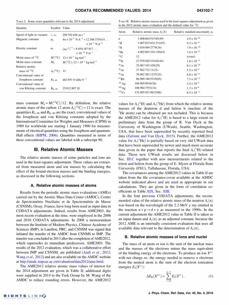
TABLE II. Relative atomic masses used in the least-squares adjustment as givenin the 2012 atomic mass evaluation and the defined value for 12C
Atom Relative atomic mass ArðXÞ Relative standard uncertainty ur
n 1.008 664 915 85(49) 4:9× 10−101H 1.007 825 032 231(93) 9:3× 10−113H 3.016 049 2779(24) 7:9× 10−104He 4.002 603 254 130(63) 1:6× 10−1112C 12 (exact)28Si 27.976 926 534 65(44) 1:6× 10−1136Ar 35.967 545 105(29) 8:1× 10−1038Ar 37.962 732 11(21) 5:5× 10−940Ar 39.962 383 1237(24) 6:0× 10−1187Rb 86.909 180 5319(65) 7:5× 10−11107Ag 106.905 0916(26) 2:4× 10−8109Ag 108.904 7553(14) 1:3× 10−8133Cs 132.905 451 9615(86) 6:5× 10⁻¹¹
CODATA RECOMMENDED VALUES: 2014 043102-7
J. Phys. Chem. Ref. Data, Vol. 45, No. 4, 2016
For a neutral atom we have n= 0 and ΔEBðX0+Þ= 0; for a barenucleus n= Z. In the 2014 least-squares adjustment, we use theremoval energies expressed in terms of wave numbers given by
ΔEBð1H+Þ=hc= 1:096 787 717 4307ð10Þ× 107 m−1,
ΔEBð3H+Þ=hc= 1:097 185 4390ð13Þ× 107 m−1 ,
ΔEBð4He2+Þ=hc= 6:372 195 4487ð28Þ× 107 m−1,
ΔEBð12C6+Þ=hc= 83:083 962ð72Þ× 107 m−1,
ΔEBð12C5+Þ=hc= 43:563 345ð72Þ× 107 m−1,
ΔEBð28Si13+Þ=hc= 420:608ð19Þ× 107 m−1 ,
which follow from the data tabulated in Table III. In that table,the value for 1H is from Jentschura et al. (2005), and the restare from the NIST online Atomic Spectra Database (ASD,2015), in which the value for 3H is based on a calculation byKotochigova (2006). In general, because of the relatively smallsize of the uncertainties of the ionization energies given inTable III, any correlations that might exist among them or withother data used in the CODATA-14 are unimportant. How-ever, there is a significant covariance between the two carbonbinding-energy values, because a large part of the uncertaintyis due to common uncertainties in the lower ionization stages;this yields the correlation coefficient
r½EBð12C5+Þ=hc,EBð12C6+Þ=hc�= 0:999 976. (2)
The relative atomic mass of an atom, its ions, the relativeatomic mass of the electron, and the relative atomic mass
equivalent of the binding energy of the removed electrons arerelated according to
ArðXÞ=ArðXn+Þ+ nArðeÞ−ΔEBðXn+Þmuc2
, (3)
where mu =mð12CÞ=12 is the unified atomic mass constant.Equation (3) is the form of the observational equation for ArðXÞused in previous adjustments with ArðXn+Þ and ArðeÞ taken asadjusted constants with the binding-energy term taken to beexact. However, because for 28Si the binding-energy un-certainty is not negligible compared with the uncertainty ofArð28SiÞ, we adopt the following new approach for treatingbinding energies in all calculations in which they are required.Since the binding energies are known most accurately in termsof their wave number equivalents, and since R∞ =α2mec=2hand me =ArðeÞmu, one can write
ΔEBðXn+Þmuc2
=α2ArðeÞ2R∞
ΔEBðXn+Þhc
. (4)
Thus, in the 2014 adjustment we replace the binding-energy termin Eq. (3) byEq. (4) and take the binding energyΔEBðXn+Þ=hc asboth an input datum and an adjusted constant, thereby obtaininga new form of observational equation for ArðXÞ expressed solelyin terms of adjusted constants. Although this requires takingbinding energies as input data rather than exactly knownquantities, it allows all binding-energy uncertainties and co-variances to be properly taken into account. This new form ofobservational equation is used for the AME2012 values ofArð1HÞ, Arð3HÞ, Arð4HeÞ, and Arð28SiÞ, and the new way oftreating binding energies is used in the observational equationsfor a number of frequency ratios; see Table XXIV, Sec. XIII.
C. Relative atomic mass of the deuteron, triton,and helion
We consider here the recent data of the University ofWashington and Florida State University groups mentionedabove relevant to the determination of the relative atomicmasses of the nuclei of the 2H (deuterium D), 3H (tritium T),and 3He atoms, or deuteron d, triton t, and helion h, respec-tively. The data are cyclotron frequency ratios obtained ina Penning trap and it is these ratios that are used as input data inthe adjustment to determine ArðdÞ, ArðtÞ, and ArðhÞ, which aretaken as adjusted constants. These new results became avail-able shortly before the 31 December 2014 closing date of theadjustment and were published in 2015.
The UWash group reports as the final values of the cyclotronfrequency ratios d and h to 12C6+ (Zafonte and Van Dyck, 2015)
ωcðdÞωcð12C6+Þ= 0:992 996 654 743ð20Þ ½2:0× 10−11� , (5)
ωcðhÞωcð12C6+Þ= 1:326 365 862 193ð19Þ ½1:4× 10⁻¹¹� . (6)
These ratios are correlated because of the image chargecorrection applied to each; based on the published uncertaintybudgets and additional information provided by Van Dyck(2015), their correlation coefficient is
TABLE III. Ionization energies for 1H, 3H, 3He, 4He, 12C, and 28Si
Atom or ion EI=hcð107 m−1Þ1H 1.096 787 717 4307(10)3H 1.097 185 4390(13)3He+ 4.388 891 936(3)4He 1.983 106 6637(20)4He+ 4.389 088 785(2)12C 0.908 2045(10)12C+ 1.966 74(7)12C2+ 3.862 410(10)12C3+ 5.201 758(15)12C4+ 31.624 233(2)12C5+ 39.520 616 7(5)28Si 0.657 4776(25)28Si+ 1.318 381(3)28Si2+ 2.701 393(7)28Si3+ 3.640 931(6)28Si4+ 13.450 7(2)28Si5+ 16.5559(15)28Si6+ 19.867(8)28Si7+ 24.492(14)28Si8+ 28.318(6)28Si9+ 32.374(3)28Si10+ 38.406(6)28Si11+ 42.216 3(6)28Si12+ 196.610 389(16)
043102-8 MOHR, NEWELL, AND TAYLOR
J. Phys. Chem. Ref. Data, Vol. 45, No. 4, 2016
r½ωcðdÞ=ωcð12C6+Þ,ωcðhÞ=ωcðC6+Þ�= 0:306. (7)
The relative atomic masses follow from the relations
ωcðdÞωcð12C6+Þ=
Arð12C6+Þ6ArðdÞ , (8)
ωcðhÞωcð12C6+Þ=
Arð12C6+Þ3ArðhÞ , (9)
where
Arð12C6+Þ= 12− 6ArðeÞ+ΔEBð12C6+Þmuc2
, (10)
which takes into account the definition Arð12CÞ= 12.An overview of the University of Washington Penning trap
mass spectrometer (UW-PTMS), which was developed overseveral decades, is given by Zafonte and Van Dyck (2015);a discussion of the various experimental effects that caninfluence UW-PTMS cyclotron frequency measurements isgiven by Van Dyck, et al. (2006). The later paper also reportsa preliminary value of Arð2HÞ based on the analysis ofωcðdÞ=ωcð12C6+Þ data obtained in three early data runs. Thefinal result of the UWash deuterium measurements given inEq. (5) is based on 10 data runs, each of which yields onefrequency ratio and lasted more than a month when the timerequired to check all experimental effects is included. Correc-tions for six significant experimental effects are applied to eachof the 10 ratios before their weighted mean is calculated. Thelargest of these by far is that for image charge; its fractionalmagnitude is −245× 10−12 for each ratio. Each correction hasan uncertainty, but since the 9:9× 10⁻¹² relative standarduncertainty ur of the image charge correction is the same foreach ratio, it is omitted from the individual ratio uncertainties.Rather, Zafonte and Van Dyck (2015) take it into account bycombining it with the uncertainty ur = 17:4× 10⁻¹² of theweighted mean calculated without the image charge uncer-tainty, thereby obtaining the 20 parts in 1012 final uncertainty.
Although there were seven successful helion runs todetermine ωcðhÞ=ωcð12C6+Þ, Zafonte and Van Dyck (2015)decided to exclude runs three and four from their final analysisbecause they were found to contain two 12C6+ ions instead ofone. To avoid the problem of isolating a single 12C6+ ion, theyused a single 12C5+ ion in the three other runs and scaled theresults using the well-known values of Arð12C5+Þ and Arð12C6+Þwithout adding any significant uncertainty to what they wouldhave obtained if a 12C6+ ion had been used. Zafonte and VanDyck (2015) treat the five individual ωcðhÞ=ωcð12C6+Þ fre-quency ratios as they did the 10 ωcðdÞ=ωcð12C6+Þ ratios; thefractional image charge correction is −515× 10−12 withur = 8:9× 10⁻¹², for the weighted mean of the five ratiosur = 11:2× 10⁻¹², and for the final value ur = 14× 10−12.
The cyclotron frequency ratios of HD+ to 3He+ and to treported by the FSU group are (Myers et al., 2015)
ωcðHD+Þωcð3He+Þ= 0:998 048 085 153ð48Þ ½4:8× 10⁻¹¹� , (11)
ωcðHD+ÞωcðtÞ = 0:998 054 687 288ð48Þ ½4:8× 10⁻¹¹� . (12)
As for the two UWash ratios, these ratios are correlated, but inthis case because of the correction to account for imbalancebetween the cyclotron radii of the two ions. Based on thepublished uncertainty budgets and additional informationprovided by Myers (2015), their correlation coefficient is
r½ωcðHD+Þ=ωcð3He+Þ,ωcðHD+Þ=ωcðtÞ�= 0:875. (13)
The relevant equations for these data are
ωcðHD+Þωcð3He+Þ=
Arð3He+ÞArðHD+Þ , (14)
ωcðHD+ ÞωcðtÞ =
ArðtÞArðHD+ Þ , (15)
where
Arð3He+Þ=ArðhÞ+ArðeÞ−EIð3He+Þmuc2
, (16)
EIð3He+Þ=hc= 43 888 919:36ð3Þ m−1 , (17)
ArðHD+ Þ=ArðpÞ+ArðdÞ+ArðeÞ−EIðHD+ Þmuc2
, (18)
EIðHD+Þ=hc= 13 122 468:415ð6Þ m−1 . (19)
The ionization wave number in Eq. (17) is from Table III, andthe value in Eq. (19) is from Liu et al. (2010) and Sprecheret al. (2010).
In the FSU experiment pairs of individual ions, either HD+
and 3H+ or HD+ and 3He+, are confined at the same time ina Penning trap at 4.2 K with an applied magnetic flux densityof 8.5 T. The cyclotron frequency of one ion centered in thetrap in an orbit with a radius of about 45 μm is determinedwhile the other ion is kept in an outer orbit with a radius ofabout 1.1 mm to reduce perturbations on the inner ion due toCoulomb interactions. The two ions are then interchanged. Ina typical run lasting up to 10 h about 20 cyclotron frequencymeasurements are made on each ion. The temporal variation ofthe magnet flux density is accounted for by simultaneouslyfitting a fourth-order polynomial to the individual cyclotronfrequencies as a function of time. In total 34 HD+=3He+ andHD+=3H+ runs were carried out over a 5 month period. Foreach frequency ratio the standard uncertainty of the mean ofthe individual values before correction for two systematiceffects is 17× 10−12. The correction for cyclotron radiusimbalance for each is 22ð45Þ× 10−12 and for the polarizabilityof the HD+ ion, 94× 10−12 with negligible uncertainty. Thesetwo uncertainty components lead to the final uncertainty foreach of 48× 10−12.
Since the cyclotron frequencies in Eqs. (11) and (12) areboth measured with reference to the same molecular ion HD+
and there is a sizable correlation coefficient between thefrequency ratio measurements, Myers et al. (2015) obtaina value for the ratio ωcð3H+Þ=ωcð3He+Þ with only one-halfthe 4:8× 10⁻¹¹ uncertainty of that for either of the ratiosdetermined with HD+. They are thus able to deduce for themass difference between the tritium and helium-3 atoms,mð3HÞ−
CODATA RECOMMENDED VALUES: 2014 043102-9
J. Phys. Chem. Ref. Data, Vol. 45, No. 4, 2016
mð3HeÞ= 1:995 934 ð7Þ× 10−5 u= 18 592:01 ð7Þ eV=c2,whichhas a significantly smaller uncertainty than any other value.
The value of Arð3HeÞ deduced by Myers et al. (2015)from their data, 3.016 029 322 43(19), exceeds the value de-duced by Zafonte and Van Dyck (2015) from their data,3.016 029 321 675(43), by 3.9 times the standard uncertaintyof their difference udiff or 3:9σ. (Throughout the paper, σ asused here is the standard uncertainty udiff of the differencebetween two values.) How this disagreement is treated in the2014 adjustment is discussed in Sec. XIII. The THe-Trapexperiment currently underway at the Max-Planck-Institutfur Kernphysik (MPIK), Heidelberg, Germany, the aim ofwhich is to determine the ratio Arð3HÞ=Arð3HeÞ in order todetermine the Q-value of tritium, may clarify the cause ofthis discrepancy; see Diehl et al. (2011) and Streubel et al. (2014).
IV. Atomic Transition Frequencies
Comparison of theory and experiment for transition frequen-cies in hydrogen, deuterium, and muonic hydrogen providesinformation on the Rydberg constant, and on the charge radii ofthe proton and deuteron. Hyperfine splittings in hydrogen andfine-structure splittings in helium are also briefly considered.
A. Hydrogen and deuterium transition frequencies,the Rydberg constant R‘, and the proton
and deuteron charge radii rp, rd
The transition frequency between states i and i0 with energylevels Ei and Ei0 in hydrogen or deuterium is given by
hνii0 =Ei0 −Ei . (20)
The energy levels are given by
Ei =−α2mec2
2n2ið1+ δiÞ=−R∞hc
n2ið1+ δiÞ , (21)
where R∞ is the Rydberg constant, ni is the principal quantumnumber of state i, and δi, where jδij≪1, contains the details ofthe theory of the energy level.
1. Theory of hydrogen and deuterium energy levels
References to the original works are generally omitted; thesemay be found in earlier detailed CODATA reports, in Eides,Grotch, and Shelyuto (2001, 2007), and in Sapirstein andYennie (1990). Uncertainties we assign to the individualtheoretical contributions are categorized as either correlatedor uncorrelated. Correlations we consider arise in two forms.One case is where the uncertainties are mainly of the formC=n3i , where C is the same for all states with the same L and j.Such uncertainties are denoted by u0, while the uncorrelateduncertainties are denoted by ui. The other correlations weconsider are those between corrections for the same state indifferent isotopes, where the correction only depends on themass of the isotope. Calculations of the uncertainties of theenergy levels and the corresponding correlation coefficientsare described in Sec. IV.A.1.l.
a. Dirac eigenvalue. The Dirac eigenvalue for an electronbound to a stationary point nucleus is
ED = f ðn, jÞmec2 , (22)
where
f ðn, jÞ="1+
ðZαÞ2ðn− δÞ2
#−1=2, (23)
n and j are the principal and total angular-momentum quantumnumbers of the bound state,
δ= j+12−��
j+12
�2 − ðZαÞ2�1=2
, (24)
and Z is the charge number of the nucleus.For a nucleus with a finite mass mN, we have
EMðHÞ=Mc2 + ½ f ðn, jÞ− 1�mrc2 − ½ f ðn, jÞ− 1�2m
2r c
2
2M
+1− δℓ0
κð2ℓ+ 1ÞðZαÞ4m3
r c2
2n3m2N
+⋯ (25)
for hydrogen or
EMðDÞ=Mc2 + ½ f ðn, jÞ− 1�mrc2 − ½ f ðn, jÞ− 1�2m
2r c
2
2M
+1
κð2ℓ+ 1ÞðZαÞ4m3
r c2
2n3m2N
+⋯ (26)
for deuterium, where ℓ is the nonrelativistic orbital angular-momentum quantum number, δℓ0 is the Kronecker delta,
κ= ð−1Þj−ℓ+1=2ðj+ 12Þ is the angular-momentum-parity quantum
number, M =me +mN, and mr =memN=ðme +mNÞ is the re-duced mass.
b. Relativistic recoil. The leading relativistic-recoil correc-tion, to lowest order in Zα and all orders in me=mN, is(Erickson, 1977; Sapirstein and Yennie, 1990)
ES =m3
r
m2emN
ðZαÞ5πn3
mec2
×
13δℓ0lnðZαÞ−2 − 8
3lnk0ðn, ℓÞ− 1
9δℓ0 − 7
3an
− 2m2
N −m2e
δℓ0
�m2
Nln
me
mr
�−m2
e ln
mN
mr
���, (27)
where
an =−2"ln
2n
�+Xn
i= 1
1i+ 1− 1
2n
#δℓ0 +
1− δℓ0
ℓðℓ+ 1Þð2ℓ + 1Þ .
(28)
Values we use for the Bethe logarithms lnk0ðn, ℓÞ in Eqs. (27),(38), and (65) are given in Table IV.
Additional contributions to lowest order in the mass ratioand of higher order in Zα are
ER =me
mN
ðZαÞ6n3
mec2½D60 +D72Zα ln2ðZαÞ−2 +⋯� , (29)
where
043102-10 MOHR, NEWELL, AND TAYLOR
J. Phys. Chem. Ref. Data, Vol. 45, No. 4, 2016
D60 =
�4 ln 2− 7
2
�δℓ0 +
�3− ℓðℓ+ 1Þ
n2
�2ð1− δℓ0Þ
ð4ℓ2 − 1Þð2ℓ + 3Þ ,(30)
D72 =− 1160π
δℓ0 . (31)
The uncertainty in the relativistic recoil correction is takento be
½0:1δℓ0 + 0:01ð1− δℓ0Þ�ER . (32)
Covariances follow from the ðme=mNÞ=n3 scaling of theuncertainty.
c. Nuclear polarizability. For the nuclear polarizability inhydrogen, we use
EPðHÞ=−0:070ð13Þh δℓ0n3
kHz, (33)
and for deuterium
EPðDÞ=−21:37ð8Þh δℓ0n3
kHz. (34)
Presumably the polarizability effect is negligible for states ofhigher ℓ in either hydrogen or deuterium.
d. Self energy. The one-photon self energy of an electronbound to a stationary point nucleus is
Eð2ÞSE =
α
π
ðZαÞ4n3
FðZαÞmec2 , (35)
where
FðZαÞ=A41lnðZαÞ−2 +A40 +A50ðZαÞ+A62ðZαÞ2ln2ðZαÞ−2 +A61ðZαÞ2lnðZαÞ−2
+GSEðZαÞðZαÞ2 , (36)
with
A41 =43δℓ0 , (37)
A40 =− 43ln k0ðn, ℓÞ+ 10
9δℓ0 − 1
2κð2ℓ+ 1Þð1− δℓ0Þ , (38)
A50 =
�13932
− 2ln2�πδℓ0 , (39)
A62 =−δℓ0 , (40)
A61 =
h4�1+
12+⋯+
1n
�+283ln 2− 4 ln n
− 601180
− 7745n2
�δℓ0 +
n2 − 1n2
� 215
+13δj 12
�δℓ1,
+½96n2 − 32ℓðℓ + 1Þ�ð1− δℓ0Þ
3n2ð2ℓ− 1Þð2ℓÞð2ℓ+ 1Þð2ℓ+ 2Þð2ℓ+ 3Þ . (41)
Values for GSEðαÞ in Eq. (36) are listed in Table V. SeeCODATA-10 for details. The uncertainty of the self-energycontribution to a given level is due to the uncertainty ofGSEðαÞlisted in that table and is taken to be type un.
Following convention, FðZαÞ is multiplied by the reduced-mass factor ðmr=meÞ3, except the magnetic-moment term−1=½2κð2ℓ+ 1Þ� in A40 which is instead multiplied by thefactor ðmr=meÞ2, and the argument ðZαÞ−2 of the logarithms isreplaced by ðme=mrÞðZαÞ−2.
e. Vacuum polarization. The stationary point nucleussecond-order vacuum-polarization level shift is
Eð2ÞVP =
α
π
ðZαÞ4n3
HðZαÞmec2 , (42)
where HðZαÞ=Hð1ÞðZαÞ+HðRÞðZαÞ,
Hð1ÞðZαÞ=V40 +V50ðZαÞ+V61ðZαÞ2lnðZαÞ−2
+Gð1ÞVPðZαÞðZαÞ2 , (43)
HðRÞðZαÞ=GðRÞVP ðZαÞðZαÞ2 , (44)
with
V40 =− 415
δℓ0,
V50 =548
πδℓ0,
V61 =− 215
δℓ0 .
(45)
Values of Gð1ÞVPðZαÞ are given in Table VI, and
TABLE IV. Relevant values of the Bethe logarithms ln k0ðn, ℓÞ
n S P D
1 2.984 128 5562 2.811 769 893 −0:030 016 7093 2.767 663 6124 2.749 811 840 −0:041 954 895 −0:006 740 9396 2.735 664 207 −0:008 147 2048 2.730 267 261 −0:008 785 04312 −0:009 342 954
TABLE V. Values of the function GSEðαÞ
n S1=2 P1=2 P3=2 D3=2 D5=2
1 −30:290 240ð20Þ2 −31:185 150ð90Þ −0:973 50ð20Þ −0:486 50ð20Þ3 −31:047 70ð90Þ4 −30:9120ð40Þ −1:1640ð20Þ −0:6090ð20Þ 0.031 63(22)6 −30:711ð47Þ 0.034 17(26)8 −30:606ð47Þ 0.007 940(90) 0.034 84(22)12 0.009 130(90) 0.035 12(22)
CODATA RECOMMENDED VALUES: 2014 043102-11
J. Phys. Chem. Ref. Data, Vol. 45, No. 4, 2016
GðRÞVP ðZαÞ=
1945
− π2
27
�δℓ0 +
116
− 31π2
2880
�πðZαÞδℓ0 +⋯ .
(46)
Higher-order terms are negligible. We multiply Eq. (42) byðmr=meÞ3 and include a factor of ðme=mrÞ in the argument ofthe logarithm in Eq. (43).
Vacuum polarization from μ+μ− pairs is
Eð2ÞμVP =
α
π
ðZαÞ4n3
�− 415
δℓ0
�me
mμ
�2mr
me
�3
mec2 , (47)
and hadronic vacuum polarization is given by
Eð2ÞhadVP = 0:671ð15ÞEð2Þ
μVP . (48)
Uncertainties are of type u0. The muonic and hadronic vacuum-polarization contributions are negligible for higher-ℓ states.
f. Two-photon corrections. The two-photon correction is
Eð4Þ =�α
π
�2ðZαÞ4n3
mec2Fð4ÞðZαÞ , (49)
where
Fð4ÞðZαÞ=B40 +B50ðZαÞ+B63ðZαÞ2ln3ðZαÞ−2
+B62ðZαÞ2ln2ðZαÞ−2 +B61ðZαÞ2lnðZαÞ−2
+B60ðZαÞ2 +B72ðZαÞ3ln2ðZαÞ−2
+B71ðZαÞ3lnðZαÞ−2 +B70ðZαÞ3+⋯ , (50)
with
B40 =
�3π2
2ln 2− 10π2
27− 2179
648− 94ζð3Þ
�δℓ0
+
�π2ln 22
− π2
12− 197144
− 3ζð3Þ4
�1− δℓ0
κð2ℓ+ 1Þ , (51)
B50 =−21:554 47ð13Þδℓ0 , (52)
B63 =− 827
δℓ0 , (53)
B62 =169
�7160
− ln 2+ γ+ψðnÞ− ln n− 1n+
14n2
�δℓ0
+427
n2 − 1n2
δℓ1 , (54)
B61 =
413 58164 800
+4NðnSÞ
3+2027π2
864− 616 ln 2
135− 2π2ln 2
3
+40 ln22
9+ ζð3Þ
+
304135
− 32 ln 29
��34+ γ+ψðnÞ− ln n− 1
n+
14n2
��δℓ0
+
�43NðnPÞ+ n2 − 1
n2
� 31405
+13δj 12
− 827
ln 2��
δℓ1 .
(55)
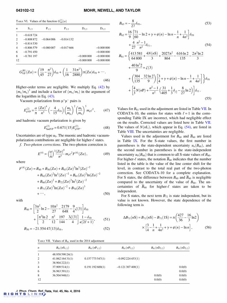
Values for B61 used in the adjustment are listed in Table VII. InCODATA-10, the entries for states with ℓ= 1 in the corre-sponding Table IX are incorrect, which had negligible effecton the results. Corrected values are listed here in Table VII.The values of NðnLÞ, which appear in Eq. (54), are listed inTable VIII. The uncertainties are negligible.
Values used in the adjustment for B60 and B60 are listedin Table IX. For the S-state values, the first number inparentheses is the state-dependent uncertainty unðB60Þ, andthe second number in parentheses is the state-independentuncertainty u0ðB60Þ that is common to all S-state values of B60.For higher-ℓ states, the notation B60 indicates that the numberlisted in the table is the value of the line center shift for thelevel, in contrast to the total real part of the two-photoncorrection. See CODATA-10 for a complete explanation.For S states, the difference between B60 and B60 is negligiblecompared to the uncertainty of the value of B60. The un-certainties of B60 for higher-ℓ states are taken to beindependent.
For S states, the next term B72 is state independent, but itsvalue is not known. However, the state dependence of thefollowing term is
ΔB71ðnSÞ=B71ðnSÞ−B71ð1SÞ=π
42736
− 163ln2
�
×
h34− 1n+
14n2
+ γ+ψðnÞ− ln ni, (56)
TABLE VI. Values of the function Gð1ÞVPðαÞ
n S1=2 P1=2 P3=2 D3=2 D5=2
1 −0:618 7242 −0:808 872 −0:064 006 −0:014 1323 −0:814 5304 −0:806 579 −0:080 007 −0:017 666 −0:000 0006 −0:791 450 −0:000 0008 −0:781 197 −0:000 000 −0:000 00012 −0:000 000 −0:000 000
TABLE VII. Values of B61 used in the 2014 adjustment
n B61ðnS1=2Þ B61ðnP1=2Þ B61ðnP3=2Þ B61ðnD3=2Þ B61ðnD5=2Þ
1 48.958 590 24(1)2 41.062 164 31(1) 0.157 775 547(1) −0:092 224 453ð1Þ3 38.904 222(1)4 37.909 514(1) 0.191 192 600(1) −0:121 307 400ð1Þ 0.0(0)6 36.963 391(1) 0.0(0)8 36.504 940(1) 0.0(0) 0.0(0)12 0.0(0) 0.0(0)
043102-12 MOHR, NEWELL, AND TAYLOR
J. Phys. Chem. Ref. Data, Vol. 45, No. 4, 2016
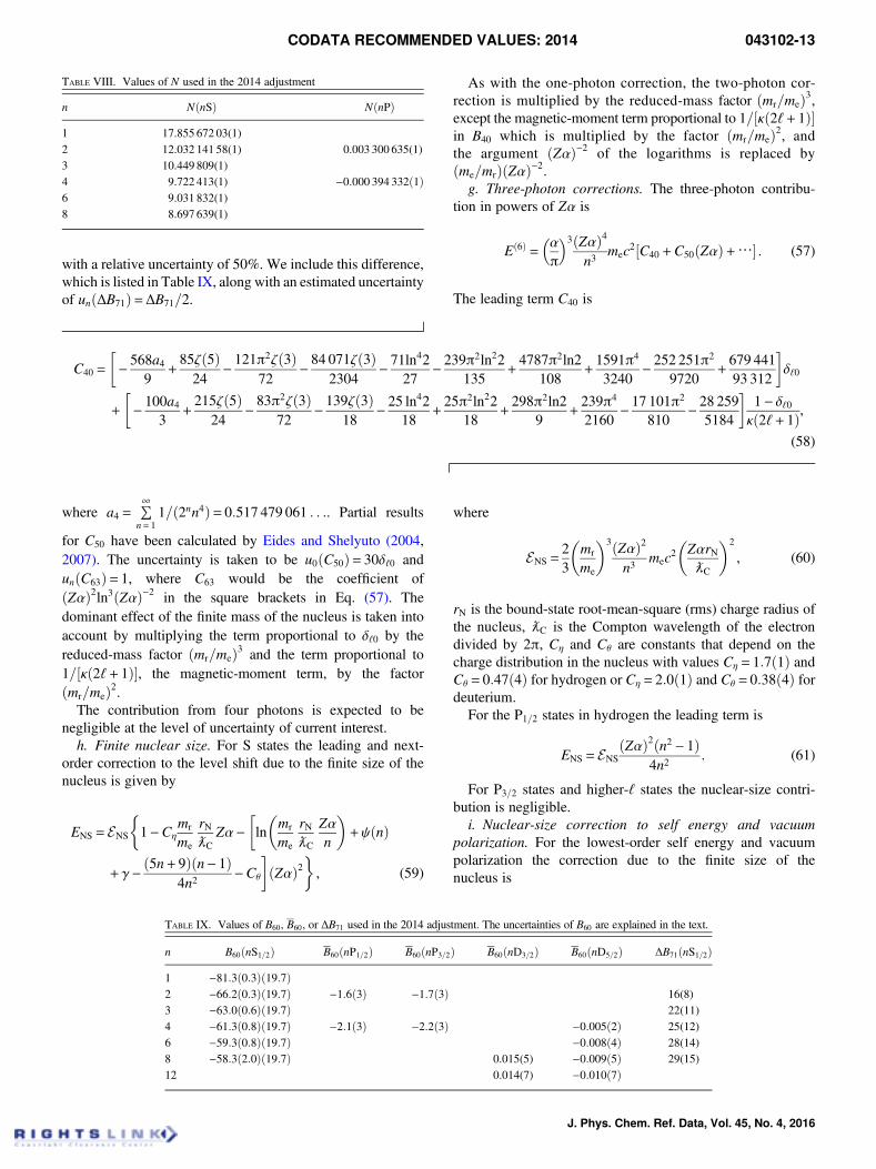
with a relative uncertainty of 50%. We include this difference,which is listed in Table IX, along with an estimated uncertaintyof unðΔB71Þ=ΔB71=2.
As with the one-photon correction, the two-photon cor-rection is multiplied by the reduced-mass factor ðmr=meÞ3,except the magnetic-moment term proportional to 1=½κð2ℓ+ 1Þ�in B40 which is multiplied by the factor ðmr=meÞ2, andthe argument ðZαÞ−2 of the logarithms is replaced byðme=mrÞðZαÞ−2.
g. Three-photon corrections. The three-photon contribu-tion in powers of Zα is
Eð6Þ =�α
π
�3ðZαÞ4n3
mec2½C40 +C50ðZαÞ+⋯� . (57)
The leading term C40 is
C40 =
�− 568a4
9+85ζð5Þ24
− 121π2ζð3Þ72
− 84 071ζð3Þ2304
− 71ln4227
− 239π2ln22135
+4787π2ln2
108+1591π4
3240− 252 251π2
9720+679 44193 312
�δℓ0
+
�− 100a4
3+215ζð5Þ
24− 83π2ζð3Þ
72− 139ζð3Þ
18− 25 ln42
18+25π2ln22
18+298π2ln2
9+239π4
2160− 17 101π2
810− 28 259
5184
�1− δℓ0
κð2ℓ+ 1Þ,(58)
where a4 =P∞n= 1
1=ð2nn4Þ= 0:517 479 061 . . .. Partial results
for C50 have been calculated by Eides and Shelyuto (2004,2007). The uncertainty is taken to be u0ðC50Þ= 30δℓ0 andunðC63Þ= 1, where C63 would be the coefficient ofðZαÞ2ln3ðZαÞ−2 in the square brackets in Eq. (57). Thedominant effect of the finite mass of the nucleus is taken intoaccount by multiplying the term proportional to δℓ0 by thereduced-mass factor ðmr=meÞ3 and the term proportional to1=½κð2ℓ + 1Þ�, the magnetic-moment term, by the factorðmr=meÞ2.
The contribution from four photons is expected to benegligible at the level of uncertainty of current interest.
h. Finite nuclear size. For S states the leading and next-order correction to the level shift due to the finite size of thenucleus is given by
ENS = ENS
1−Cη
mr
me
rNƛC
Zα−�ln
mr
me
rNƛC
Zαn
�+ψðnÞ
+ γ− ð5n+ 9Þðn− 1Þ4n2
−Cθ
�ðZαÞ2
�, (59)
where
ENS =23
mr
me
�3ðZαÞ2n3
mec2
ZαrNƛC
�2
, (60)
rN is the bound-state root-mean-square (rms) charge radius ofthe nucleus, ƛC is the Compton wavelength of the electrondivided by 2π, Cη and Cθ are constants that depend on thecharge distribution in the nucleus with values Cη = 1:7ð1Þ andCθ = 0:47ð4Þ for hydrogen or Cη = 2:0ð1Þ and Cθ = 0:38ð4Þ fordeuterium.
For the P1=2 states in hydrogen the leading term is
ENS = ENSðZαÞ2ðn2 − 1Þ
4n2. (61)
For P3=2 states and higher-ℓ states the nuclear-size contri-bution is negligible.
i. Nuclear-size correction to self energy and vacuumpolarization. For the lowest-order self energy and vacuumpolarization the correction due to the finite size of thenucleus is
TABLE VIII. Values of N used in the 2014 adjustment
n NðnSÞ NðnPÞ
1 17.855 672 03(1)2 12.032 141 58(1) 0.003 300 635(1)3 10.449 809(1)4 9.722 413(1) −0:000 394 332ð1Þ6 9.031 832(1)8 8.697 639(1)
TABLE IX. Values of B60, B60, or ΔB71 used in the 2014 adjustment. The uncertainties of B60 are explained in the text.
n B60ðnS1=2Þ B60ðnP1=2Þ B60ðnP3=2Þ B60ðnD3=2Þ B60ðnD5=2Þ ΔB71ðnS1=2Þ
1 −81:3ð0:3Þð19:7Þ2 −66:2ð0:3Þð19:7Þ −1:6ð3Þ −1:7ð3Þ 16(8)3 −63:0ð0:6Þð19:7Þ 22(11)4 −61:3ð0:8Þð19:7Þ −2:1ð3Þ −2:2ð3Þ −0:005ð2Þ 25(12)6 −59:3ð0:8Þð19:7Þ −0:008ð4Þ 28(14)8 −58:3ð2:0Þð19:7Þ 0.015(5) −0:009ð5Þ 29(15)12 0.014(7) −0:010ð7Þ
CODATA RECOMMENDED VALUES: 2014 043102-13
J. Phys. Chem. Ref. Data, Vol. 45, No. 4, 2016
ENSE =
�4ln2− 23
4
�αðZαÞENSδℓ0 , (62)
and
ENVP =34αðZαÞENSδℓ0 , (63)
respectively.j. Radiative-recoil corrections. Corrections for radiative-
recoil effects are
ERR =m3
r
m2emN
αðZαÞ5π2n3
mec2δℓ0
×
�6ζð3Þ− 2π2ln2+
35π2
36− 448
27
+23πðZαÞln2ðZαÞ−2 +⋯
�. (64)
The uncertainty is ðZαÞlnðZαÞ−2 relative to the square bracketswith a factor of 10 for u0 and 1 for un. Corrections for higher-ℓstates are negligible.
k. Nucleus self energy. The nucleus self energy correctionfor S states is
ESEN =4Z2αðZαÞ4
3πn3m3
r
m2N
c2"ln
mN
mrðZαÞ2!δℓ0 − lnk0ðn, ℓÞ
#,
(65)
with an uncertainty u0 given by Eq. (65) with the factor in thesquare brackets replaced by 0.5. For higher-ℓ states, thecorrection is negligible.
l. Total energy and uncertainty. The energy EXðnLjÞ of alevel (where L= S, P, . . . and X =H, D) is the sum ofthe various contributions listed above. Uncertainties in thefundamental constants that enter the theoretical expressionsare taken into account through the formalism of the least-squares adjustment. To take uncertainties in the theory intoaccount, a correction δXðnLjÞ that is zero with an uncertaintythat is the rms sum of the uncertainties of the individualcontributions
u2½δXðnLjÞ�=X
i
½u20iðXnLjÞ+ u2niðXnLjÞ� , (66)
where u0iðXnLjÞ and uniðXnLjÞ are the components of un-certainty u0 and un of contribution i, is added to the level. Thecorrections δXðnLjÞ, which includes their uncertainties, aretaken as input data in the least-squares adjustment. Covari-ances are taken into account by calculating all the covariancesand including them in the input data for the adjustment.
Covariances of the δs for a given isotope are
u½δXðn1LjÞ, δXðn2LjÞ�=X
i
u0iðXn2LjÞu0iðXn1LjÞ . (67)
Covariances between δs for hydrogen and deuterium for statesof the same n are
u½δHðnLjÞ, δDðnLjÞ�=X
i= ficg½u0iðHnLjÞu0iðDnLjÞ
+ uniðHnLjÞuniðDnLjÞ� , (68)
and for n1�n2
u½δHðn1LjÞ, δDðn2LjÞ�=X
i= ficgu0iðHn1LjÞu0iðDn2LjÞ , (69)
where the summation is over the uncertainties common tohydrogen and deuterium.
Values of u½δXðnLjÞ� are given in Table XVI of Sec. XIII,and the non-negligible covariances of the δs are given ascorrelation coefficients in Table XVII.
m. Transition frequencies between levels with n= 2 andthe fine-structure constant α. QED predictions for hydrogentransition frequencies between levels with n= 2 are obtainedfrom a least-squares adjustment that does not include anexperimental value for the transitions being calculated (itemsA39, A40:1, or A40:2 in Table XVI), where the constants ArðeÞ,ArðpÞ, ArðdÞ, and α are assigned the 2014 values. Theresults are
νHð2P1=2 − 2S1=2Þ= 1 057 843:7ð2:1Þ kHz ½2:0× 10−6�,νHð2S1=2 − 2P3=2Þ= 9 911 197:8ð2:1Þ kHz ½2:1× 10⁻⁷�,νHð2P1=2 − 2P3=2Þ= 10 969 041:530ð41Þ kHz ½3:7× 10⁻⁹�,
(70)
which are consistent with the experimental results given inTable XVI.
Data for the hydrogen and deuterium transitions yield avalue for the fine-structure constant α, which follows from aleast-squares adjustment that includes all the transition fre-quency data in Table XVI, the 2014 adjusted values of ArðeÞ,ArðpÞ, and ArðdÞ, but no other input data for α. The result is
α−1 = 137:035 992ð55Þ ½4:0× 10−7� , (71)
and is also given in Table XX.
2. Experiments on hydrogen and deuterium
Table X gives the hydrogen and deuterium transitionfrequencies used to determine the Rydberg constant R∞, itemsA26 to A48 in Table XVI, Sec. XIII. The only differencebetween this table and the corresponding Table XI inCODATA-10 is that the value for the 1S1=2 − 2S1=2 hydrogentransition frequency obtained by the group at the Max-Planck-Institut fur Quantenoptik (MPQ), Garching, Germany, used inthe 2010 adjustment is superseded by two new values obtainedby the same group but with significantly smaller uncertainties(first two entries of Table X):
νHð1S1=2 − 2S1=2Þ= 2 466 061 413 187:035ð10Þ½4:2× 10⁻¹⁵� , (72)
νHð1S1=2 − 2S1=2Þ= 2 466 061 413 187:018ð11Þ½4:4× 10⁻¹⁵� . (73)
043102-14 MOHR, NEWELL, AND TAYLOR
J. Phys. Chem. Ref. Data, Vol. 45, No. 4, 2016
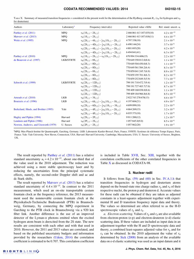
The result reported by Parthey et al. (2011) has a relativestandard uncertainty ur = 4:2× 10⁻¹⁵, about one-third that ofthe value used in the 2010 adjustment. The reduction wasachieved using a more stable spectroscopy laser and byreducing the uncertainties from the principal systematiceffects, namely, the second-order Doppler shift and ac anddc Stark shifts.
The result reported by Matveev et al. (2013) has a relativestandard uncertainty of 4:4× 10⁻¹⁵. In contrast to the 2011measurement, which used an on-site transportable cesiumfountain clock as the frequency reference, the 2013 measure-ment used the nonmovable cesium fountain clock at thePhyisikalisch-Technische Budesanstalt (PTB) in Braunsch-weig, Germany, by connecting the MPQ experiment inGarching to the PTB clock in Braunschweig via a 920 kmfiber link. Another difference is the use of an improveddetector of the Lyman-α photons emitted when the excitedhydrogen atom beam is deexcited from the 2S state. The newresults are consistent with each other and with that used in2010. However, the 2011 and 2013 values are correlated, andbased on the published uncertainty budgets and informationprovided by the researchers (Udem, 2014) the correlationcoefficient is estimated to be 0.707. This correlation coefficient
is included in Table XVII, Sec. XIII, together with thecorrelation coefficients of the other correlated frequencies inTable X as discussed in CODATA-98.
3. Nuclear radii
It follows from Eqs. (59) and (60) in Sec. IV.A.1.h thattransition frequencies in hydrogen and deuterium atomsdepend on the bound-state rms charge radius rp and rd of theirrespective nuclei, the proton p and deuteron d. Accurate valuesfor these radii can be obtained if they are taken as adjustedconstants in a least-squares adjustment together with experi-mental H and D transition frequency input data and theory.The values so determined are often referred to as the H-Dspectroscopic values of rp and rd.
a. Electron scattering.Values of rp and rd are also availablefrom electron-proton (e-p) and electron-deuteron (e-d) elasticscattering data. If these values are included as input data in anadjustment together with the H and D spectroscopic data andtheory, a combined least-squares adjusted value for rp and forrd can be obtained. In the 2010 adjustment the value of rddetermined by Sick (2008) from an analysis of the availabledata on e-d elastic scattering was used as an input datum and it
TABLE X. Summary of measured transition frequencies ν considered in the present work for the determination of the Rydberg constant R∞ (νH for hydrogen and νDfor deuterium)
Authors Laboratorya Frequency interval(s) Reported value ν/kHz Rel. stand. uncert. ur
Parthey et al. (2011) MPQ νHð1S1=2 − 2S1=2Þ 2 466 061 413 187.035(10) 4:2× 10⁻¹⁵
Matveev et al. (2013) MPQ νHð1S1=2 − 2S1=2Þ 2 466 061 413 187.018(11) 4:4× 10⁻¹⁵
Weitz et al. (1995) MPQ νHð2S1=2 − 4S1=2Þ− 14νHð1S1=2 − 2S1=2Þ 4 797 338(10) 2:1× 10⁻⁶
νHð2S1=2 − 4D5=2Þ− 14νHð1S1=2 − 2S1=2Þ 6 490 144(24) 3:7× 10⁻⁶
νDð2S1=2 − 4S1=2Þ− 14νDð1S1=2 − 2S1=2Þ 4 801 693(20) 4:2× 10⁻⁶
νDð2S1=2 − 4D5=2Þ− 14νDð1S1=2 − 2S1=2Þ 6 494 841(41) 6:3× 10⁻⁶
Parthey et al. (2010) MPQ νDð1S1=2 − 2S1=2Þ− νHð1S1=2 − 2S1=2Þ 670 994 334.606(15) 2:2× 10⁻¹¹
de Beauvoir et al. (1997) LKB/SYRTE νHð2S1=2 − 8S1=2Þ 770 649 350 012.0(8.6) 1:1× 10⁻¹¹
νHð2S1=2 − 8D3=2Þ 770 649 504 450.0(8.3) 1:1× 10⁻¹¹
νHð2S1=2 − 8D5=2Þ 770 649 561 584.2(6.4) 8:3× 10⁻¹²
νDð2S1=2 − 8S1=2Þ 770 859 041 245.7(6.9) 8:9× 10⁻¹²
νDð2S1=2 − 8D3=2Þ 770 859 195 701.8(6.3) 8:2× 10⁻¹²
νDð2S1=2 − 8D5=2Þ 770 859 252 849.5(5.9) 7:7× 10⁻¹²
Schwob et al. (1999) LKB/SYRTE νHð2S1=2 − 12D3=2Þ 799 191 710 472.7(9.4) 1:2× 10⁻¹¹
νHð2S1=2 − 12D5=2Þ 799 191 727 403.7(7.0) 8:7× 10⁻¹²
νDð2S1=2 − 12D3=2Þ 799 409 168 038.0(8.6) 1:1× 10⁻¹¹
νDð2S1=2 − 12D5=2Þ 799 409 184 966.8(6.8) 8:5× 10⁻¹²
Arnoult et al. (2010) LKB νHð1S1=2 − 3S1=2Þ 2 922 743 278 678(13) 4:4× 10⁻¹²
Bourzeix et al. (1996) LKB νHð2S1=2 − 6S1=2Þ− 14νHð1S1=2 − 3S1=2Þ 4 197 604(21) 4:9× 10⁻⁶
νHð2S1=2 − 6D5=2Þ− 14νHð1S1=2 − 3S1=2Þ 4 699 099(10) 2:2× 10⁻⁶
Berkeland, Hinds, and Boshier (1995) Yale νHð2S1=2 − 4P1=2Þ− 14νHð1S1=2 − 2S1=2Þ 4 664 269(15) 3:2× 10⁻⁶
νHð2S1=2 − 4P3=2Þ− 14νHð1S1=2 − 2S1=2Þ 6 035 373(10) 1:7× 10⁻⁶
Hagley and Pipkin (1994) Harvard νHð2S1=2 − 2P3=2Þ 9 911 200(12) 1:2× 10⁻⁶
Lundeen and Pipkin (1986) Harvard νHð2P1=2 − 2S1=2Þ 1 057 845.0(9.0) 8:5× 10⁻⁶
Newton, Andrews, and Unsworth (1979) U. Sussex νHð2P1=2 − 2S1=2Þ 1 057 862(20) 1:9× 10⁻⁵
aMPQ: Max-Planck-Institut fur Quantenoptik, Garching, Germany. LKB: Laboratoire Kastler-Brossel, Paris, France. SYRTE: Systemes de reference Temps Espace, Paris,France. Yale: Yale University, New Haven, Connecticut, USA. Harvard: Harvard University, Cambridge, Massachusetts, USA. U. Sussex: University of Sussex, Brighton,UK.
CODATA RECOMMENDED VALUES: 2014 043102-15
J. Phys. Chem. Ref. Data, Vol. 45, No. 4, 2016
is again used as an input datum in the 2014 adjustment. Thatvalue is rd = 2:130ð10Þ fm.
The e-p scattering value of rp is more problematic. Two suchvalues were used in the 2010 adjustment: rp = 0:895ð18Þ fmand rp = 0:8791ð79Þ fm. The first is due to Sick (2008) basedon his analysis of the data then available. The second is froma seminal experiment, described in detail by Bernauer et al.(2014), carried out at the Johannes Gutenberg UniversitatMainz (or simply the University of Mainz), Mainz, Germany,with the Mainz microtron electron-beam accelerator MAMI.Both values are discussed in CODATA-10, as is the significantdisagreement of the H-D spectroscopic and e-p scatteringvalues of rp with the value determined from spectroscopicmeasurements of the Lamb shift in muonic hydrogen. Thecause of the disagreement remains unknown, and we reviewthe current situation in the following section and in Sec.XIII.B.2.
To assist in deciding what scattering value or values of rp touse in the 2014 adjustment, the Task Group invited a numberof researchers active in the field to attend its annual meeting inNovember 2014. It also helped organize the Workshop on theDetermination of the Fundamental Constants held in Eltville,Germany, in February 2015, the proceedings of which arepublished in J. Phys. Chem. Ref. Data 44(3) (2015). A pointof concern at these meetings was how best to extract rp fromthe MAMI data and from the combination of the MAMI datawith the remaining available data. As a result of the discussionsat these meetings two pairs of knowledgeable researchers,J. Arrington and I. Sick, and J. C. Bernauer and M.O. Distler,provided the Task Group with their best estimate of rp fromall the available data. The Arrington-Sick value, rp =0:879ð11Þ fm, has been published (Arrington and Sick,2015) but was initially transmitted to the Task Group as aprivate communication in 2015; the Bernauer-Distler value,rp = 0:880ð11Þ fm, was also transmitted to the Task Group in2015 as a private communication but has not been published.The two values are highly consistent even though differentapproaches and assumptions were used to obtain them. Wetherefore adopt as the e-p scattering-data input datum for rp inthe 2014 adjustment
rp = 0:879ð11Þ ½1:3× 10⁻²� fm, (74)
which is the weighted mean of the two values, but theuncertainty is the average of their uncertainties since eachvalue was based on essentially the same data.
The Task Group well recognizes that Eq. (74) is not the lastword on the subject and that the topic remains one of activeinterest; see, for example, the papers by Kraus et al. (2014),Arrington (2015), Lorenz et al. (2015), and Sick (2015).Particularly noteworthy is the paper by Lee, Arrington, andHill (2015), which did not become available until well after the31 December closing date of the 2014 adjustment, that pro-vides a new and improved analysis to obtain rp = 0:895ð20Þ fmfrom the MAMI data, rp = 0:916ð24Þ fm from the remainingavailable data but not including the MAMI data, and rp =0:904ð15Þ fm by combining these two values. Three recentpapers by Griffioen, Carlson and Maddox (2016), Higinbotham
et al. (2016), and Horbatsch and Hessels (2016) obtain resultsconsistent with the smaller muonic hydrogen radius in Eq. (78).However, Bernauer and Distler (2016) point out a number ofproblems with the analyses in these papers.
b. Isotope shift and the deuteron-proton radius difference.From a comparison of experiment and theory for the hydrogen-deuterium isotope shift, one can extract a value for thedifference of the squares of the charge radii for the deuteronand proton, based on the 2014 recommended values, given by
r2d − r2p = 3:819 48ð37Þ fm2 . (75)
The corresponding result based on the 2010 recommendedvalues,
r2d − r2p = 3:819 89ð42Þ fm2 , (76)
differs from the current value due mainly to the change in therelative atomic mass of the electron used to evaluate thetheoretical expression for the isotope shift. The electron massappears as an overall factor as can be seen from the leadingterm (Jentschura et al., 2011)
Δf1S−2S,d −Δf1S−2S,p ≈− 34R∞c
me
md−me
mp
�. (77)
c. Muonic hydrogen. The first reported value of rp fromspectroscopic measurements of the Lamb shift in the muonichydrogen atom μ-p obtained by the Charge Radius Experimentwith Muonic Atoms (CREMA) collaboration (Pohl et al.,2010) and the problem, now often called the “proton radiuspuzzle,” that resulted from its significant disagreement with thescattering and spectroscopic values is discussed in CODATA-10. As a result of this inconsistency the Task Group decidedthat the initial μ-p value of rp should be omitted from the 2010adjustment and the 2010 recommended value should be basedon only the two available e-p scattering values (see previoussection) and the H-D spectroscopic data and theory. Conse-quently the disagreement of the μ-p value with the 2010recommended value was 7σ and with the H-D spectroscopicvalue, 4:4σ.
The μ-p Lamb-shift experiment employs pulsed laserspectroscopy at a special muon beam line at the protonaccelerator of the Paul Scherrer Institute (PSI), Villigen,Switzerland. Muonic atoms in the 2S state (lifetime 1 μs) areformed when muons from the beam strike a gaseous H2 target,a 5 ns near-resonance laser pulse (tunable from 50 THz to 55THz) induces transitions to the 2P state (lifetime 8.5 ps), theatoms decay to the 1S ground state by emitting 1.9 keV Kαx rays, and a resonance curve is obtained by counting thenumber of x rays as a function of laser frequency. (Because ofthe large electron vacuum-polarization effect in μ-p, the 2S1/2
level is far below both the 2P1/2 and 2P3/2 levels.)The transition initially measured was 2S1/2ðF = 1Þ−
2P3=2ðF = 2Þ at 50 THz or 6 μm. More recently, the CREMAcollaboration reported their result for the transition2S1/2ðF = 0Þ− 2P3=2ðF = 1Þ at 55 THz or 5:5 μm, as well astheir reevaluation of the 50 THz data (Antognini et al., 2013b).
043102-16 MOHR, NEWELL, AND TAYLOR
J. Phys. Chem. Ref. Data, Vol. 45, No. 4, 2016
This reevaluation reduced the original frequency by 0.53 GHzand its uncertainty from 0.76 GHZ to 0.65 GHz. By com-parison, the uncertainty of the 55 THz frequency is 1.05 GHz.
The theory that relates the muonic hydrogen Lamb-shifttransition frequencies to rp reflects the calculations and criticalinvestigations of many researchers, and a number of issueshave been resolved since the closing date of the 2010 adjust-ment; a detailed review is given by Antognini et al. (2013a).Using the theory in this paper the CREMA collaborationreports, in the same paper in which they give their twomeasured transition frequencies (Antognini et al., 2013b),the following value as the best estimate of rp from muonichydrogen:
rp = 0:840 87ð39Þ fm. (78)
This may be compared with the muonic hydrogen valuerp = 0:841 69ð66Þ fm available for consideration in the 2010adjustment based on the 2S1/2ðF = 1Þ− 2P3=2ðF = 2Þ transitionfrequency before reevaluation and the theory as it existed atthe time. Because the new result in Eq. (78) is smaller andhas a smaller uncertainty than this value and that neither theH-D data nor theory have changed significantly, it is notsurprising that the disagreement still persists and that the TaskGroup has decided to omit the μ-p result for rp in the 2014adjustment. Indeed, the disagreement of the value in Eq. (78)with the 2014 CODATA recommended value 0.8751(61) fm is5:6σ and with the H-D spectroscopic value 0.8759(77) fmis 4:5σ.
The negative effect of including the value of rp in Eq. (78) asan input datum in the 2014 adjustment and why the TaskGroup concluded that it should be excluded is discussedfurther in Sec. XIII.B.2. However, we do point out here the twofollowing facts.
First, if the least-squares adjustment that leads to the value ofα−1 given in Eq. (71) is carried out with the value in Eq. (78)included as an input datum, the result is α−1 = 137:035 876ð35Þ[2:6× 10⁻⁷], which differs from the 2014 recommended valueby 3:5σ.
Second, Karshenboim (2014) has proposed a differentapproach to the calculation of the next-to-leading higher-order proton-size contribution to the theory of the muonichydrogen Lamb shift than was used by Antognini et al.(2013b) to obtain the value of rp in Eq. (78). The approachchanges the value in Eq. (78) to rp = 0:840 22ð56Þ fm(Karshenboim, 2014), for which the disagreement with the2014 CODATA recommended value is 5:7σ and with theH-D spectroscopic value is 4:6σ. [The slightly different valuerp = 0:840 29ð55Þ fm was subsequently published after theclosing date of the 2014 adjustment by Karshenboim et al.(2015).] Because this value of rp is consistent with the value inEq. (78), because the disagreement for the two values with the2014 CODATA recommended value and H-D spectroscopicvalue are very nearly the same, and because the suggestedapproach has not yet been widely accepted, we have used thevalue of rp in Eq. (78) for our discussion here and analysis inSec. XIII.B.2.
A recent review of the proton radius puzzle is given byCarlson (2015).
B. Hyperfine structure and fine structure
In principle, together with theory, hyperfine-structuremeasurements other than in muonium, and fine-structuremeasurements other than in hydrogen and deuterium, couldprovide accurate values of some constants, most notably thefine-structure constant α. Indeed, it has long been the hopethat a competitive value of α could be obtained from experi-mental measurements and theoretical calculations of 4He fine-structure transition frequencies. However, as discussed inCODATA-10, no such data were available for the 2010adjustment and this is also the case for the 2014 adjustment.
For completeness, we note that there have been significantimprovements in both the theory and experimental determi-nation of the hyperfine splitting in positronium [see Adkinset al. (2015), Eides and Shelyuto (2015), Ishida (2015), andMiyazaki et al. (2015) and the references cited therein]. Also,Marsman, Horbatsch, and Hessels (2015a, 2015b) have foundthat the measured values of helium fine-structure transitionfrequencies can be significantly influenced by quantum-mechanical interference between neighboring resonances evenif separated by thousands of natural linewidths. The shifts theycalculated for reported experimental values of the 23P1 − 23P2fine-structure interval in 4He improve their agreement withtheory.
V. Magnetic Moments and g-factors
The magnetic-moment vector of a charged lepton is
μℓ = gℓe
2mℓ
s , (79)
where ℓ= e, μ, or τ, gℓ is the g-factor, with the convention thatit has the same sign as the charge of the particle, e is the(positive) unit charge, mℓ is the lepton mass, and s is its spin.Since the spin has projection eigenvalues of sz =±ℏ=2, themagnetic moment is defined to be
μℓ =gℓ2
eℏ2mℓ
, (80)
and the Bohr magneton is just
μB =eℏ2me
. (81)
The g-factor differs from the Dirac value of 2 because of thelepton magnetic-moment anomaly aℓ defined by
jgℓj= 2ð1+ aℓÞ . (82)
The theoretical value of the anomaly is given by QED, pre-dominately electroweak, and predominantly strong-interactioneffects denoted by
aℓðthÞ= aℓðQEDÞ+ aℓðweakÞ+ aℓðhadÞ , (83)
respectively.
CODATA RECOMMENDED VALUES: 2014 043102-17
J. Phys. Chem. Ref. Data, Vol. 45, No. 4, 2016
A. Electron magnetic-moment anomaly ae
and the fine-structure constant α
A value for the fine-structure constant α is obtained byequating theory and experiment for the electron magnetic-moment anomaly.
1. Theory of ae
The QED contribution to the electron anomaly is
aeðQEDÞ=A1 +A2ðme=mμÞ+A2ðme=mτÞ+A3ðme=mμ,me=mτÞ , (84)
where the mass-dependent terms arise from vacuum-polarization loops. Each term may be expanded in powers ofthe fine-structure constant as
Ai =X∞
n= 1Að2nÞi
�α
π
�n, (85)
where Að2Þ2 =Að2Þ
3 =Að4Þ3 = 0.
The mass-independent terms Að2nÞ1 are known accurately
through sixth order:
Að2Þ1 =
12, (86)
Að4Þ1 =−0:328 478 965 579 193 . . . , (87)
Að6Þ1 = 1:181 241 456 . . . . (88)
Recent numerical evaluations have yielded values for theeighth- and tenth-order coefficients (Aoyama et al., 2014)
Að8Þ1 =−1:912 98ð84Þ , (89)
Að10Þ1 = 7:795ð336Þ . (90)
Higher-order coefficients are assumed to be negligible.Mass-dependent coefficients for the electron, based on the
CODATA-14 values of the mass ratios, are
Að4Þ2 ðme=mμÞ= 5:197 386 76ð23Þ× 10−7 → 24:182× 10−10ae ,
(91)
Að4Þ2 ðme=mτÞ= 1:837 98ð33Þ× 10−9 → 0:086× 10−10ae , (92)
Að6Þ2 ðme=mμÞ=−7:373 941 71ð24Þ× 10−6
→ − 0:797× 10−10ae ,(93)
Að6Þ2 ðme=mτÞ=−6:5830ð11Þ× 10−8 → − 0:007× 10−10ae .
(94)
Additional series expansions in the mass ratios yield (Kurzet al., 2014a)
Að8Þ2 ðme=mμÞ= 9:161 970 83ð33Þ× 10−4 → 0:230× 10−10ae ,
(95)
Að8Þ2 ðme=mτÞ= 7:4292ð12Þ× 10−6 → 0:002× 10−10ae: (96)
A numerical calculation gives the next term (Aoyama et al.,2012b)
Að10Þ2 ðme=mμÞ=−0:003 82ð39Þ→ − 0:002× 10−10ae . (97)
Additional terms have been calculated, but are negligible at thecurrent level of accuracy; see, for example, Aoyama et al.(2014) and Kurz et al. (2014a).
All contributing terms of each order in α are combined toyield the total coefficients in the series
aeðQEDÞ=X∞
n= 1Cð2nÞ
e
�α
π
�n, (98)
with
Cð2Þe = 0:5,
Cð4Þe =−0:328 478 444 00 . . . ,
Cð6Þe = 1:181 234 017 . . . ,
Cð8Þe =−1:912 06ð84Þ,
Cð10Þe = 7:79ð34Þ ,
(99)
where higher-order coefficients are negligible.The electroweak contribution, calculated as in CODATA-98
but with present values of GF and sin2θW (see Sec. XII), is
aeðweakÞ= 0:029 73ð23Þ× 10−12 = 0:2564ð20Þ× 10−10ae .(100)
The hadronic contribution is the sum
aeðhadÞ= aLO,VPe ðhadÞ+ aNLO,VPe ðhadÞ+ aLLe ðhadÞ+⋯ ,
(101)
where aLO,VPe ðhadÞ and aNLO,VPe ðhadÞ are the leading order andnext-to-leading order (with an additional photon or electronloop) hadronic vacuum-polarization corrections given byNomura and Teubner (2013)
aLO,VPe ðhadÞ= 1:866ð11Þ× 10−12 , (102)
aNLO,VPe ðhadÞ=−0:2234ð14Þ× 10−12 , (103)
and aNNLO,VPe ðhadÞ is the next-to-next-to-leading order vacuum-polarization correction (Kurz et al., 2014b)
aNNLO,VPe ðhadÞ= 0:0280ð10Þ× 10−12 , (104)
and where aLLe ðhadÞ is the hadronic light-by-light scatteringterm given by Prades, de Rafael, and Vainshtein (2010)
aLLe ðhadÞ= 0:035ð10Þ× 10−12 . (105)
The total hadronic contribution is
aeðhadÞ= 1:734ð15Þ× 10−12 = 14:95ð13Þ× 10−10ae . (106)
043102-18 MOHR, NEWELL, AND TAYLOR
J. Phys. Chem. Ref. Data, Vol. 45, No. 4, 2016
The theoretical value is the sum of all the terms:
aeðthÞ= aeðQEDÞ+ aeðweakÞ+ aeðhadÞ , (107)
and has the standard uncertainty
u½aeðthÞ�= 0:037× 10−12 = 0:32× 10−10ae , (108)
where the largest contributions to the uncertainty are from the8th- and 10th-order QED terms. This uncertainty is taken intoaccount in the least-squares adjustment by writing
aeðthÞ= aeðαÞ+ δe , (109)
where 0:000ð37Þ× 10−12 is the input datum for δe. It isnoteworthy that the uncertainty of aeðthÞ is significantlysmaller than the uncertainty of the most accurate experimentalvalue (see following section), which is 2:4× 10⁻¹⁰ae.
2. Measurements of ae
Two experimental values of ae obtained using a Penningtrap were initially included in CODATA-10. The first is theclassic 1987 result from the University of Washingtondiscussed in CODATA-98 with a relative standard uncertaintyur = 3:7× 10⁻⁹ and which assumes that CPT invariance holdsfor the electron-positron system (Van Dyck, Schwinberg, andDehmelt, 1987). The second is the much more accurate 2008result from Harvard University discussed in CODATA-10with ur = 2:4× 10⁻¹⁰ (Hanneke, Fogwell, and Gabrielse,2008). These results are items B22:1 and B22:2 in TableXVIII, Sec. XIII, with identifications UWash-87 and HarvU-08; the values of α that can be inferred from them based on thetheory of ae discussed in the previous section are given inTable XX, Sec. XIII.A. The University of Washington resultwas not included in the final adjustment on which theCODATA 2010 recommended values are based because ofits comparatively low weight and is also omitted from the 2014final adjustment. It is only considered to help provide anoverall picture of the data available for the determination of the2014 recommended value of α.
B. Muon magnetic-moment anomaly aμ
Only the measured value of the muon magnetic-momentanomaly was included in the 2010 adjustment of the con-stants due to concerns about some aspects of the theory. Theconcerns still remain, thus the Task Group decided not toemploy the theoretical expression for aμ in the 2014 adjustment.The theory and measurement of aμ and the reasons for the TaskGroup decision are presented in the following sections.
1. Theory of aμ
The relevant mass-dependent terms are
Að4Þ2 ðmμ=meÞ= 1:094 258 3092ð72Þ→ 5:06× 10−3aμ , (110)
Að4Þ2 ðmμ=mτÞ= 0:000 078 079ð14Þ→ 3:61× 10−7aμ , (111)
Að6Þ2 ðmμ=meÞ= 22:868 379 98ð17Þ→ 2:46× 10−4aı , (112)
Að6Þ2 ðmμ=mτÞ= 0:000 360 63ð11Þ→ 3:88× 10−9aμ , (113)
Að8Þ2 ðmμ=meÞ= 132:6852ð60Þ→ 3:31× 10−6aμ , (114)
Að8Þ2 ðmμ=mτÞ= 0:042 4941ð53Þ→ 1:06× 10−9aμ , (115)
Að10Þ2 ðmμ=meÞ= 742:18ð87Þ→ 4:30× 10−8aμ , (116)
Að10Þ2 ðmμ=mτÞ=−0:068ð5Þ→ − 3:94× 10−12aμ , (117)
Að6Þ3 ðmμ=me,mμ=mτÞ= 0:000 527 762ð94Þ
→ 5:67× 10−9aμ , (118)
Að8Þ3 ðmμ=me,mμ=mτÞ= 0:062 72ð4Þ→ 1:57× 10−9aμ . (119)
Að10Þ3 ðmμ=me,mμ=mτÞ= 2:011ð10Þ→ 1:17× 10−10aμ . (120)
New mass-dependent contributions reported since CODATA-10 are Eqs. (114), (116), (117), (119), and (120) from Aoyamaet al. (2012a) and Eq. (115) from Kurz et al. (2014a).
The total for aμðQEDÞ is
aμðQEDÞ=X∞
n= 1Cð2nÞ
e
�α
π
�n, (121)
with
Cð2Þμ = 0:5,
Cð4Þμ = 0:765 857 423ð16Þ,
Cð6Þμ = 24:050 509 82ð27Þ,
Cð8Þμ = 130:8774ð61Þ,
Cð10Þμ = 751:92ð93Þ .
(122)
Based on the 2014 recommended value of α, this yields
aμðQEDÞ= 0:001 165 847 188 58ð87Þ ½7:4× 10⁻¹⁰� , (123)
where an uncertainty of 0:8× 10⁻¹² is included to account foruncalculated 12th-order terms (Aoyama et al., 2012a).
As for the electron, there are additional contributions:
aμðthÞ= aμðQEDÞ+ aμðweakÞ+ aμðhadÞ . (124)
The primarily electroweak contribution is (Czarnecki, Marciano,and Vainshtein, 2003; Gnendiger, Stockinger, and Stockinger-Kim, 2013)
aμðweakÞ= 154ð1Þ× 10−11 . (125)
Separate contributions (lowest-order vacuum polarization, next-to-lowest-order, and light-by-light) to the hadronic term are
aμðhadÞ= aLO,VPμ ðhadÞ+ aNLO,VPμ ðhadÞ+ aLLμ ðhadÞ+⋯ ,
(126)
CODATA RECOMMENDED VALUES: 2014 043102-19
J. Phys. Chem. Ref. Data, Vol. 45, No. 4, 2016
where (Hagiwara et al., 2011)
aLO,VPμ ðhadÞ= 6949ð43Þ× 10−11 , (127)
aNLO,VPμ ðhadÞ=−98:40ð72Þ× 10−11 , (128)
and (Jegerlehner and Nyffeler, 2009)
aLLμ ðhadÞ= 116ð40Þ× 10−11 . (129)
The total hadronic contribution is then
aμðhadÞ= 6967ð59Þ× 10−11 . (130)
In analogy with the electron we have finally
aμðthÞ= aμðQEDÞ+ 7121ð59Þ× 10−11 , (131)
with the standard uncertainty
u½aμðthÞ�= 59× 10−11 = 51× 10−11aμ . (132)
The largest contributions to the uncertainty are fromaLO,VPμ ðhadÞ and aLLμ ðhadÞ; their respective uncertainties of43× 10−11 and 40× 10−11 are nearly the same. By comparison,the 0:087× 10−11 uncertainty of aμðQEDÞ is negligible.However, the 63× 10−11 uncertainty of the experimental valueof aμ, which is discussed in the following section, and u½aμðthÞ�are nearly the same. Based on the 2014 recommended value ofα, Eq. (131) yields
aμðthÞ= 1:165 918 39ð59Þ× 10−3 (133)
for the theoretically predicted value of aμ.
2. Measurement of aμ: Brookhaven
The experimental determination of aμ at BrookhavenNational Laboratory (BNL), Upton, New York, USA, hasbeen discussed in the past four CODATA reports. The quantitymeasured is the anomaly difference frequency fa = fs − fc,where fs = jgμjðeℏ=2mμÞB=h is the muon spin-flip (or pre-cession) frequency in the applied magnetic flux density B andfc = eB=2πmμ is the corresponding muon cyclotron frequency.The flux density is eliminated from these expressions bydetermining its value using proton nuclear magnetic resonance(NMR) measurements. This means that the muon anomaly iscalculated from
aμðexpÞ= Rjμμ=μpj−R
(134)
where R= fa=f p and f p is the free proton NMR frequencycorresponding to the average flux density B seen by the muonsin their orbits in the muon storage ring.
The final value of R obtained in the experiment is, fromTable XV of Bennett et al. (2006),
R= 0:003 707 2063ð20Þ , (135)
which is used as an input datum in the 2014 adjustment and isthe same as used in the 2010 adjustment. It is datum B24 inTable XVIII with identification BNL-06. Based on this valueof R, Eq. (134), and the 2014 recommended value of μμ=μp,whose uncertainty is negligible in this context, the experimen-tal value of the muon anomaly is
aμðexpÞ= 1:165 920 89ð63Þ× 10−3 . (136)
Further, with the aid of Eq. (225), the equation for R can bewritten as
R=− aμ1+ ae
me
mμ
μeμp
, (137)
where use has been made of the relations ge =−2ð1+ aeÞ,gμ =−2ð1+ aμÞ, and ae is replaced by the theoretical expres-sion given in Eq. (109) for the observational equation. If thetheory of aμ were not problematic and used in adjustmentcalculations, then aμ in Eq. (137) would be its theoreticalexpression, which mainly depends on α. If the theory isomitted, then aμ in that equation is simply taken to be anadjusted constant. The following section discusses why theTask Group decided to do the latter.
3. Comparison of theory and experiment for aμ
The difference between the experimental value of aμ in Eq.(136) and the theoretical value in Eq. (133) is 250ð86Þ× 10−11,which is 2.9 times the standard uncertainty of the difference or2:9σ. The terms aLO,VPμ ðhadÞ and aLLμ ðhadÞ are the dominantcontributors to the uncertainty of aμðthÞ, and a smaller value ofeither will increase the disagreement while a larger value willdecrease it.
The value for aLO,VPμ ðhadÞ used to obtain aμðthÞ is6949ð43Þ× 10−11, but an equally credible value, 6923ð42Þ×10−11, is also available (Davier et al., 2011). If it is usedinstead, the discrepancy is 276ð86Þ× 10−11 or 3:2σ. Bothvalues are based on very thorough analyses using theoryand experimental data from the production of hadrons ine+e− collisions. Davier et al. (2011) also obtain the value7015ð47Þ× 10−11 using both e+ e− annihilation data and datafrom the decay of the τ into hadrons. For this value thediscrepancy is reduced to 2:1σ. A result due to Jegerlehner andSzafron (2011) also obtained using e+ e− annihilation data andτ decay data but which is only in marginal agreement with thisvalue is 6910ð47Þ× 10−11. However, it agrees with the first twovalues, which are based solely on e+ e− data. For this value thediscrepancy is 3:3σ. In a lengthy paper Benayoun et al. (2013)used the hidden local symmetry model or HLS to obtain valuesof aLO,VPμ ðhadÞ that are significantly smaller than others andthat lead to a discrepancy of between 4σ and 5σ. However,Davier and Malaescu (2013) give a number of reasons whythese values may not be reliable.
The value for aLLμ ðhadÞ used to obtain aμðthÞ is116ð40Þ× 10−11, but there are other credible values in the
043102-20 MOHR, NEWELL, AND TAYLOR
J. Phys. Chem. Ref. Data, Vol. 45, No. 4, 2016
literature. For example, Prades, de Rafael, and Vainshtein(2010) give 105ð26Þ× 10−11 while Melnikov and Vainshtein(2004) find 136ð25Þ× 10−11. A more recent value, due toNarukawa et al. (2014), is 118ð20Þ× 10−11, and the largest is188ð4Þ× 10−11 reported by Goecke, Fischer, and Williams(2013). Others range from 80ð40Þ× 10−11 to 107ð17Þ× 10−11.Recent brief overviews of aLLμ ðhadÞmay be found in Dorokhov,Radzhabov, and Zhevlakov (2014a, 2014b), Nyffeler (2014),and Adikaram et al. (2015), which describe the many obstaclesto obtaining a reliable estimate of its value. The conclusion thatemerges from these papers is that aLLμ ðhadÞ is quite modeldependent and the reliability of the estimates is questionable.Note that in calculating the value 116ð40Þ× 10−11 used to obtainEq. (133), Nyffeler (2009) adds the uncertainty componentslinearly and rounds the result up from 39× 10−11 to 40× 10−11.This result is also thoroughly discussed in the detailed review byJegerlehner and Nyffeler (2009) (see especially Table 13).
Although much work has been done over the past 4 years toimprove the theory of aμ, the discrepancy between experi-ment and theory remains at about the 3σ level. Further, thereis a significant spread in the values of aLO,VPμ ðhadÞ andaLLμ ðhadÞ, the two most problematic contributions to aμðthÞ; itis not obvious which are the best values. Expanding theuncertainty of aμðthÞ to reflect this spread would reduce itscontribution to the determination of the 2014 CODATArecommended value of aμ significantly. Expanding the un-certainties of both aμðthÞ and aμðexpÞ to reduce the discrep-ancy to an acceptable level and including both would meanthat the recommended value would cease to be a useful ref-erence value for future comparisons of theory and experi-ment; it might tend to cover up an important physics problemrather than emphasizing it. For all these reasons, the TaskGroup chose not to include aμðthÞ in the 2014 adjustment andto base the 2014 recommended value on experiment only aswas the case in 2010.
C. Proton magnetic moment in nuclearmagnetons μp/μN
The 2010 recommended value of the magnetic moment ofthe proton μp in units of the nuclear magneton μN = eℏ=2mp
has a relative standard uncertainty ur = 8:2× 10⁻⁹. It was notmeasured directly but calculated from the relation μp=μN =ðμp=μBÞ½ArðpÞ=ArðeÞ�, where ArðeÞ and ArðpÞ are adjustedconstants and μB = eℏ=2me is the Bohr magneton. The protonmagnetic moment in units of μB is calculated from μp=μB =ðμe=μBÞ=ðμe=μpÞ, where jμe=μBj= 1+ ae is extremely wellknown and μe=μp is an adjusted constant determined mainlyby the experimentally measured value of the bound-statemagnetic-moment ratio in hydrogen μeðHÞ/μpðHÞ taken as aninput datum.
Now, however, a directly determined value of μp=μN withur = 3:3× 10⁻⁹ obtained frommeasurements on a single protonin a double Penning trap at the Institut fur Physik, JohannesGutenberg Universitat Mainz (or simply the University ofMainz), Mainz, Germany, is available for inclusion in the2014 adjustment. The spin-flip transition frequency in a mag-netic flux density B is
ωs =ΔEℏ
=2μpB
ℏ, (138)
and the cyclotron frequency for the proton is
ωc =eBmp
. (139)
The ratio for the same magnetic flux density B is just
ωs
ωc=μp
μN. (140)
The value employed as an input datum in the 2014 adjust-ment is
μp
μN= 2:792 847 3498ð93Þ ½3:3× 10⁻⁹� , (141)
which is the result reported by Mooser et al. (2014) but with anadditional digit for both the value and uncertainty provided tothe Task Group by coauthor Blaum (2014). This value, whichwe identify as UMZ-14, is the culmination of an extensiveresearch program carried out over many years. Descriptions ofthe key advances made in the development of the doublePenning trap used in the experiment are given in a number ofpublications (Ulmer, Blaum et al., 2011; Ulmer, Rodegheriet al., 2011; Mooser et al., 2013; Mooser, Kracke et al., 2013;Ulmar et al., 2013).
The double Penning trap consists of a precision trap of innerdiameter 7 mm and an analysis trap of inner diameter 3.6 mmconnected by transport electrodes, all mounted in the horizon-tal bore of a superconducting magnet with B≈ 1:89 T. Storagetimes for a single proton of no less than 1 year are achieved byenclosing the entire apparatus in a sealed vacuum chambercooled to 4 Kwhere pressures below 10−14 Pa are reached. Themeasurement sequence is straightforward but its implementa-tion is complex; the cited papers should be consulted fordetails. Sputtered atoms created by electrons from a fieldemission gun hitting a polyethylene target are ionized in thecenter of the precision trap. A single proton is obtained fromthe resulting ion cloud, its cyclotron frequency of approxi-mately 29 MHz is determined, and an electromagnetic signalnear the proton’s precession frequency of approximately81 MHz is applied to it. The proton is then transported to theanalysis trap where the spin state of the proton is determinedand the proton returned to the precision trap. By varying thefrequency of the spin-flip signal and repeating the processmany times, a resonance curve of the probability Pðωs=ωcÞ asa function of ωs is obtained. Its maximum is located atωs=ωc = μp=μN. The statistical relative standard uncertainty ofthe value given in Eq. (141) is 2:6× 10⁻⁹, and the net fractionalcorrection for systematic effects is −0:64ð2:04Þ× 10−9. Thelargest contributor by far to the uncertainty of the netcorrection is the 2× 10⁻⁹ relative uncertainty assigned byMooser et al. (2014) for the possible effect of nonlinear driftsof the magnetic field.
The relationships given at the beginning of this section showhow the 2010 recommended value of μp=μN is based on therelation
CODATA RECOMMENDED VALUES: 2014 043102-21
J. Phys. Chem. Ref. Data, Vol. 45, No. 4, 2016
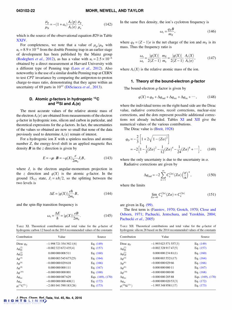
μp
μN=−ð1+ aeÞArðpÞ
ArðeÞμp
μe, (142)
which is the source of the observational equation B29 in TableXXIV.
For completeness, we note that a value of μp=μN withur = 8:9× 10⁻⁶ from the double Penning trap in an earlier stageof development has been published by the Mainz group(Rodegheri et al., 2012), as has a value with ur = 2:5× 10⁻⁶
obtained by a direct measurement at Harvard University witha different type of Penning trap (Lees et al., 2012). Alsonoteworthy is the use of a similar double Penning trap at CERNto test CPT invariance by comparing the antiproton-to-protoncharge-to-mass ratio, demonstrating that they agree within anuncertainty of 69 parts in 1012 (DiSciacca et al., 2013).
D. Atomic g-factors in hydrogenic 12Cand 28Si and Ar(e)
The most accurate values of the relative atomic mass ofthe electronArðeÞ are obtained frommeasurements of the electrong-factor in hydrogenic ions, silicon and carbon in particular, andtheoretical expressions for the g-factors. In fact, the uncertaintiesof the values so obtained are now so small that none of the datapreviously used to determine ArðeÞ remain of interest.
For a hydrogenic ion X with a spinless nucleus and atomicnumber Z, the energy-level shift in an applied magnetic fluxdensity B in the z direction is given by
E =−μ ·B=−gðXÞ e2me
JzB , (143)
where Jz is the electron angular-momentum projection inthe z direction and gðXÞ is the atomic g-factor. In theground 1S1/2 state, Jz =±ℏ=2, so the splitting between thetwo levels is
ΔE = jgðXÞj eℏ2me
B , (144)
and the spin-flip transition frequency is
ωs =ΔEℏ
= jgðXÞj eB2me
. (145)
In the same flux density, the ion’s cyclotron frequency is
ωc =qXBmX
, (146)
where qX = ðZ − 1Þe is the net charge of the ion and mX is itsmass. Thus the frequency ratio is
ωs
ωc=
jgðXÞj2ðZ − 1Þ
mX
me=
jgðXÞj2ðZ − 1Þ
ArðXÞArðeÞ , (147)
where ArðXÞ is the relative atomic mass of the ion.
1. Theory of the bound-electron g-factor
The bound-electron g-factor is given by
gðXÞ= gD +Δgrad +Δgrec +Δgns +⋯ , (148)
where the individual terms on the right-hand side are the Diracvalue, radiative corrections, recoil corrections, nuclear-sizecorrections, and the dots represent possible additional correc-tions not already included. Tables XI and XII give thenumerical values of the various contributions.
The Dirac value is (Breit, 1928)
gD =− 23
�1+ 2
ffiffiffiffiffiffiffiffiffiffiffiffiffiffiffiffiffiffiffi1− ðZαÞ2
q �
=−2h1− 1
3ðZαÞ2 − 1
12ðZαÞ4 − 1
24ðZαÞ6 +⋯
i, (149)
where the only uncertainty is due to the uncertainty in α.Radiative corrections are given by
Δgrad =−2X∞
n= 1
Cð2nÞe ðZαÞ
�α
π
�n, (150)
where the limits
limZα→0
Cð2nÞe ðZαÞ=Cð2nÞ
e (151)
are given in Eq. (99).The first term is (Faustov, 1970; Grotch, 1970; Close and
Osborn, 1971; Pachucki, Jentschura, and Yerokhin, 2004;Pachucki et al., 2005)
TABLE XII. Theoretical contributions and total value for the g-factor ofhydrogenic silicon 28 based on the 2014 recommended values of the constants
Contribution Value Source
Dirac gD −1:993 023 571 557ð3Þ Eq. (149)
Δgð2ÞSE
−0:002 328 917 47ð5Þ Eq. (157)
Δgð2ÞVP
0.000 000 234 81(1) Eq. (160)
Δgð4Þ 0.000 003 5521(17) Eq. (164)
Δgð6Þ −0:000 000 029 66 Eq. (166)
Δgð8Þ 0.000 000 000 11 Eq. (167)
Δgð10Þ −0:000 000 000 00 Eq. (168)
Δgrec −0:000 000 205 88 Eqs. (169), (170)Δgns −0:000 000 020 53ð3Þ Eq. (172)
gð28Si13+Þ −1:995 348 9581ð17Þ Eq. (173)
TABLE XI. Theoretical contributions and total value for the g-factor ofhydrogenic carbon 12 based on the 2014 recommended values of the constants
Contribution Value Source
Dirac gD −1:998 721 354 392 1ð6Þ Eq. (149)
Δgð2ÞSE
−0:002 323 672 435ð4Þ Eq. (157)
Δgð2ÞVP
0.000 000 008 511 Eq. (160)
Δgð4Þ 0.000 003 545 677(25) Eq. (164)
Δgð6Þ −0:000 000 029 618 Eq. (166)
Δgð8Þ 0.000 000 000 111 Eq. (167)
Δgð10Þ −0:000 000 000 001 Eq. (168)
Δgrec −0:000 000 087 629 Eqs. (169), (170)Δgns −0:000 000 000 408ð1Þ Eq. (172)
gð12C5+Þ −2:001 041 590 183ð26Þ Eq. (173)
043102-22 MOHR, NEWELL, AND TAYLOR
J. Phys. Chem. Ref. Data, Vol. 45, No. 4, 2016
Cð2Þe,SEðZαÞ=
12
1+
ðZαÞ26
+ ðZαÞ4�329lnðZαÞ−2+247
216− 89ln k0 − 8
3ln k3
�
+ ðZαÞ5RSEðZαÞ�, (152)
whereln k0 = 2:984 128 556, (153)
ln k3 = 3:272 806 545, (154)
RSEð6αÞ= 22:160ð10Þ , (155)
RSEð14αÞ= 20:999ð2Þ . (156)
Values for the remainder function RSEðZαÞ are based on extra-polations from numerical calculations at higher Z (Yerokhin,Indelicato, and Shabaev, 2002, 2004; Pachucki, Jentschura, andYerokhin, 2004); see also Yerokhin and Jentschura (2008,2010). In CODATA-10, the values for carbon and oxygen weretaken directly from Pachucki, Jentschura, and Yerokhin (2004).The value for silicon in Eq. (156) is obtained here by extra-polation of the data in Yerokhin, Indelicato, and Shabaev (2004)with a fitting function of the form a+ ðZαÞ½b+ clnðZαÞ−2 +d ln2ðZαÞ−2�. We thus have
Cð2Þe,SEð6αÞ= 0:500 183 606 65ð80Þ,
Cð2Þe,SEð14αÞ= 0:501 312 630ð11Þ .
(157)
The lowest-order vacuum-polarization correction consistsof a wave-function correction and a potential correction, eachof which can be separated into a lowest-order Uehling potentialcontribution and a Wichmann-Kroll higher-order contribution.The wave-function correction is (Beier, 2000; Beier et al., 2000;Karshenboim, 2000; Karshenboim, Ivanov, and Shabaev,2001a, 2001b)
Cð2Þe,VPwfð6αÞ=−0:000 001 840 3431ð43Þ,
Cð2Þe,VPwfð14αÞ=−0:000 051 091 98ð22Þ .
(158)
For the potential correction, the Uehling contribution vanishes(Beier et al., 2000), and for the Wichmann-Kroll part, we takethe value of Lee et al. (2005), which has a negligibleuncertainty from omitted binding corrections for the presentlevel of accuracy. This gives
Cð2Þe,VPpð6αÞ= 0:000 000 008 201ð11Þ,
Cð2Þe,VPpð14αÞ= 0:000 000 5467ð11Þ .
(159)
The total vacuum polarization is the sum of Eqs. (158)and (159):
Cð2Þe,VPð6αÞ=Cð2Þ
e,VPwfð6αÞ+Cð2Þe,VPpð6αÞ
=−0:000 001 832 142ð12Þ,Cð2Þ
e,VPð14αÞ=Cð2Þe,VPwfð14αÞ+Cð2Þ
e,VPpð14αÞ=−0:000 050 5452ð11Þ . (160)
One-photon corrections are the sum of Eqs. (157) and (160):
Cð2Þe ð6αÞ=Cð2Þ
e,SEð6αÞ+Cð2Þe,VPð6αÞ
= 0:500 181 774 51ð80Þ,Cð2Þ
e ð14αÞ=Cð2Þe,SEð14αÞ+Cð2Þ
e,VPð14αÞ= 0:501 262 085ð11Þ , (161)
which yields
Δgð2Þrad =−2Cð2Þ
e ðZαÞ�α
π
�=−0:002 323 663 924ð4Þ for Z = 6
=−0:002 328 682 65ð5Þ for Z = 14. (162)
The leading binding correction is known to all orders in α=π(Eides and Grotch, 1997; Czarnecki, Melnikov, and Yelkhovsky,2001):
Cð2nÞe ðZαÞ=Cð2nÞ
e
1+
ðZαÞ26
+⋯�. (163)
To order ðZαÞ4, the two-photon correction for the ground Sstate is (Pachucki et al., 2005; Jentschura et al., 2006)
Cð4Þe ðZαÞ=Cð4Þ
e
1+
ðZαÞ26
�+ ðZαÞ4
�149lnðZαÞ−2
+991 343155 520
− 29ln k0 − 4
3ln k3
+679π2
12 960− 1441π2
720ln 2+
1441480
ζð3Þ�+OðZαÞ5
=−0:328 5778ð23Þ for Z = 6
=−0:329 17ð15Þ for Z = 14, (164)
where Cð4Þe =−0:328 478 444 00 . . ., and where ln k0 and ln k3
are given in Eqs. (153) and (154). Pachucki et al. (2005) haveestimated the uncertainty due to uncalculated higher-ordercontributions to be
u½Cð4Þe ðZαÞ�= 2jðZαÞ5Cð4Þ
e RSEðZαÞj , (165)
which we use as the uncertainty. Since the remainder func-tions differ only by about 1% for carbon and silicon, the mainZ dependence of the uncertainty is given by the factor ðZαÞ5.We shall assume that the uncertainty of the two-photoncorrection is completely correlated for the two charged ions.As a consequence, information from the silicon measuredvalue will effectively be included in the theoretical predictionfor the carbon value through the least-squares adjustmentformalism.
Jentschura (2009) and Yerokhin and Harman (2013) havecalculated two-loop vacuum-polarization diagrams of the sameorder as the uncertainty in Eq. (164).
Equation (163) gives the leading two terms of the higher-loop contributions. The corrections are
CODATA RECOMMENDED VALUES: 2014 043102-23
J. Phys. Chem. Ref. Data, Vol. 45, No. 4, 2016
Cð6Þe ðZαÞ=Cð6Þ
e
1+
ðZαÞ26
+⋯�
= 1:181 611 . . . for Z = 6
= 1:183 289 . . . for Z = 14, (166)
where Cð6Þe = 1:181 234 017 . . .,
Cð8Þe ðZαÞ=Cð8Þ
e
1+
ðZαÞ26
+⋯�
=−1:912 67ð84Þ . . . for Z = 6
=−1:915 38ð84Þ . . . for Z = 14, (167)
where Cð8Þe =−1:912 06ð84Þ, and
Cð10Þe ðZαÞ=Cð10Þ
e
1+
ðZαÞ26
+⋯�
= 7:79ð34Þ . . . for Z = 6
= 7:80ð34Þ . . . for Z = 14, (168)
where Cð10Þe = 7:79ð34Þ.
Recoil of the nucleus gives a correction proportional to theelectron-nucleus mass ratio. It can be written as Δgrec =
Δgð0Þrec +Δgð2Þrec +⋯, where the two terms are zero and first orderin α=π, respectively. The first term is (Eides and Grotch, 1997;Shabaev and Yerokhin, 2002)
Δgð0Þrec =
8>>><>>>:
−ðZαÞ2 + ðZαÞ4
3
�1+
ffiffiffiffiffiffiffiffiffiffiffiffiffiffiffiffiffiffiffi1− ðZαÞ2
q �2 − ðZαÞ5PðZαÞ
9>>>=>>>;me
mN
+ ð1+ ZÞðZαÞ2me
mN
�2
=−0:000 000 087 70 . . . for Z = 6
=−0:000 000 206 04 . . . for Z = 14, (169)
where mN is the mass of the nucleus. Mass ratios, based on thecurrent adjustment values of the constants, are me=mð12C6+Þ=0:000 045 727 5 . . . and me=mð28Si14+Þ= 0:000 019 613 6 . . .[see Eqs. (10) and (3)]. For silicon, we use the interpolatedvalue Pð14αÞ= 7:162 23ð1Þ.
For Δgð2Þrec , we have
Δgð2Þrec =α
π
ðZαÞ23
me
mN+⋯
= 0:000 000 000 06 . . . for Z = 6
= 0:000 000 000 15 . . . for Z = 14. (170)
The uncertainty inΔgð2Þrec is negligible compared to that ofΔgð2Þrad.The nuclear-size correction is given to lowest order in ðZαÞ2
by (Karshenboim, 2000)
Δgns =− 83ðZαÞ4
RN
ƛC
�2
, (171)
where RN is the bound-state nuclear rms charge radius and ƛCis the Compton wavelength of the electron divided by 2π.
Glazov and Shabaev (2002) have calculated additional cor-rections within perturbation theory. Scaling their results withthe squares of updated values for the nuclear radii RN =
2:4703ð22Þ fm and RN = 3:1223ð24Þ fm from the compilationof Angeli (2004) for 12C and 28Si respectively yields
Δgns =−0:000 000 000 408ð1Þ for 12C,
Δgns =−0:000 000 020 53ð3Þ for 16Si . (172)
Tables XI and XII list the contributions discussed above andtotals given by
gð12C5+Þ=−2:001 041 590 183ð26Þ,gð28Si13+Þ=−1:995 348 9581ð17Þ . (173)
For the purpose of the least-squares adjustment, we write thetheoretical expressions for the g-factors as
gð12C5+Þ= gCðαÞ+ δC,
gð28Si13+Þ= gSiðαÞ+ δSi ,(174)
where the first term on the right-hand side of each expressiongives the calculated value along with its functional dependenceon α. The second term contains the theoretical uncertainty inthe calculated value, except for the component due to un-certainty in α, which is taken into account by the least-squaresalgorithm through the first term. We thus have
δC = 0:0ð2:6Þ× 10−11 , (175)
δSi = 0:0ð1:7Þ× 10−9 . (176)
In each case, the uncertainty is dominated by uncalculated two-loop higher-order terms, which are expected to be mainlyproportional to ðZαÞ5. For the one-loop self energy, approx-imately 85% of the remainder scales as ðZαÞ5 between C and Si[see Eqs. (155) and (156)]. As a conservative estimate, we shallassume that 80% of the uncertainty scales as ðZαÞ5 in the caseof the two-loop uncertainty. As a result, information frommeasurement of the Si g-factor will provide information aboutthe two-loop uncertainty in C and vice versa through thecovariance of the deltas in the least-squares adjustment. Thecovariance of δC and δSi is
uðδC, δSiÞ= 3:4× 10⁻²⁰ , (177)
which corresponds to a correlation coefficient ofrðδC, δSiÞ= 0:79.
2. Measurements of g(12C5+) and g(28Si13+)
As discussed at the start of Sec. V.D, recent measurementsof the electron g-factor in hydrogenic carbon and silicontogether with theory provide a value of ArðeÞ with anuncertainty so small that the data used in the CODATA 2010adjustment to determine ArðeÞ are no longer competitive andneed not be considered. As indicated at the end of that section,the experimental quantities actually determined are the ratiosof the electron spin precession (or spin-flip) frequency in
043102-24 MOHR, NEWELL, AND TAYLOR
J. Phys. Chem. Ref. Data, Vol. 45, No. 4, 2016
hydrogenic carbon and silicon ions to the cyclotron frequencyof the ions, both in the same magnetic flux density. The resultused in the 2014 adjustment for hydrogenic silicon is
ωsð28Si13+Þωcð28Si13+Þ
= 3912:866 064 84ð19Þ ½4:8× 10⁻¹¹� . (178)
This value, determined by the group at the Max-Planck-Institut fur Kernphysik (MPIK), Heidelberg, Germany, isbased on additional information including a detailed uncer-tainty budget provided to the Task Group by the experimenters(Sturm, 2015). The information was needed to calculate thecovariance between the silicon result and the MPIK carbonresult discussed below. The value in Eq. (178) differs slightlyfrom that published by the MPIK group (Sturm et al., 2013) asa consequence of the group’s reassessment of several smallcorrections for systematic effects (Sturm, 2015). The netfractional correction applied to the uncorrected ratio to obtainthe final ratio given by Sturm et al. (2013) is −638:9× 10⁻¹²
while the net fractional correction applied to obtain Eq. (178)is −678:5× 10⁻¹². The largest of these corrections by far,−659ð33Þ× 10−12, is due to image charge and the next largest,−20ð10Þ× 10−12, is due to frequency pulling. The statisticalrelative uncertainty of eight individual measurements is33× 10−12. We identify the result in Eq. (178) as MPIK-15.
Both the silicon and carbon ratios were obtained using theMPIK triple cylindrical Penning trap operating at B= 3:8 T andin thermal contact with a liquid helium bath. This trap is similarin design and operation to the double Penning trap used todirectly measure μp=μN as discussed in Sec. V.C. The first stageof the experiment occurs in the creation trap in which ions arecreated; the second stage is carried out in the analysis trap wherethe spin state of a single ion is determined; the third stage occursin the precision trap where the cyclotron frequency is measuredand a spin flip is attempted by applying a 105 GHz microwavesignal. The ion is transferred back to the analysis trap where thespin state of the ion is again determined, thereby determining ifthe spin-flip attempt in the precision trap was successful. Theprocess is then repeated. The development of the trap andassociated measurement techniques over a number of years thathas allowed uncertainties below 5 parts in 1011 to be achievedare discussed in several papers (Blaum et al., 2009; Sturm et al.,2010; Sturm, Wagner, Schabinger, and Blaum, 2011; Ulmer,Blaum et al., 2011) and results using 28Si13+ that reflectexperimental improvements have been reported (Sturm, Wag-ner, Schabinger, Zatorski et al., 2011; Schabinger et al., 2012;Sturm et al., 2013).
For hydrogenic carbon we use
ωsð12C5+Þωcð12C5+Þ= 4376:210 500 87ð12Þ ½2:8× 10⁻¹¹� , (179)
which is also based on additional information supplied to theTask Group (Sturm et al., 2015) at the same time as that forsilicon and similar in nature. The high-accuracy carbon resultwas first published in a letter to Nature (Sturm et al., 2014) anddiffers slightly from Eq. (179) but the value subsequentlypublished in the detailed report on the experiment is the same
(Kohler et al., 2015). The net fractional correction applied tothe uncorrected ratio is −283:3× 10⁻¹², with the largestcomponents being for image charge and frequency pulling at−282:4:× 10−12 and 2:20× 10−12, respectively. The statisti-cal relative uncertainty of the individual measurements is23× 10−12. The detailed report gives a comprehensive discus-sion of the MPIK trap including many possible systematiceffects and their uncertainties. We identify the result in Eq.(179) as MPIK-15.
The carbon and silicon frequency ratios in Eqs. (178) and(179) are correlated. Based on the detailed uncertainty budgetsfor the two experiments supplied to the Task Group (Sturm,2015) the correlation coefficient is
r
�ωsð12C5+Þωcð12C5+Þ,
ωsð28Si13+Þωcð28Si13+Þ
�= 0:347, (180)
which is mostly due to the image charge correction.The frequency ratios are related to the ion and electron
masses by
ωsð12C5+Þωcð12C5+Þ=−gð
12C5+Þ10ArðeÞ
�12− 5ArðeÞ+ΔEBð12C5+Þ
muc2
�, (181)
and
ωsð28Si13+Þωcð28Si13+Þ
=−geð28Si13+Þ
14ArðeÞ Arð28Si13+Þ , (182)
where Arð28Si13+Þ is taken to be an adjusted constant and isrelated to the input datum Arð28SiÞ by [see Eq. (3)]
Arð28Si13+Þ=Arð28SiÞ− 13ArðeÞ+ΔEBð28Si13+Þmuc2
. (183)
With the aid of Eq. (4) this becomes the observational equationfor Arð28Si13+Þ, which is B19 in Table XXIV. BecauseArð12CÞ= 12 exactly, such an additional observational equa-tion is unnecessary for carbon; Eq. (181) becomes theobservational equation for ωsð12C5+Þ=ωcð12C5+Þ simply byusing Eq. (4) to modify its last term (see B15 in Table XXIV).
The silicon frequency ratio yields for the relative atomicmass of the electron
ArðeÞ= 0:000 548 579 909 19ð46Þ ½8:3× 10⁻¹⁰� , (184)
and the carbon frequency ratio gives
ArðeÞ= 0:000 548 579 909 070ð17Þ ½3:1× 10⁻¹¹� . (185)
If both data are used, we obtain
ArðeÞ= 0:000 548 579 909 069ð16Þ ½2:9× 10⁻¹¹� . (186)
The slight shift in value and reduction in uncertainty inEq. (186) as compared to Eq. (185) is due to the informationabout the higher-order terms in the theory resulting from thesilicon measurement. If the covariance in the theory given byEq. (177) is taken to be zero, the result from using both
CODATA RECOMMENDED VALUES: 2014 043102-25
J. Phys. Chem. Ref. Data, Vol. 45, No. 4, 2016
measurements is the same as the result based only on thecarbon datum, within the uncertainty displayed in theequations.
We note that in the 2010 adjustment, the uncertainty ofArðpÞ was much lower than that of ArðeÞ. As a result, the ratioArðeÞ/ArðpÞ from the analysis of antiprotonic helium transi-tion frequencies together with the value for ArðpÞ provideda competitive value for ArðeÞ. Now that ArðeÞ is moreaccurately known, the value of ArðeÞ combined with the ratioArðeÞ/ArðpÞ provides a new value for ArðpÞ. However, despiteimprovement in the theory of antiprotonic helium (Korobov,Hilico, and Karr, 2014), the uncertainty of the derived valueof ArðpÞ is much too large for it to be used in the 2014adjustment.
VI. Magnetic-Moment Ratios and theMuon-Electron Mass Ratio
Free-particle magnetic-moment ratios can be obtained fromexperiments that measure moment ratios in bound states byapplying theoretical corrections relating the free moment ratiosto the bound moment ratios.
The magnetic moment of a nucleus with spin I is
μ= ge
2mpI , (187)
where g is the g-factor of the nucleus, e is the elementarycharge, and mp is the proton mass. The magnitude of themagnetic moment is defined to be
μ= gμNi , (188)
where μN = eℏ=2mp is the nuclear magneton, and i is themaximum spin projection Iz, defined by I2 = iði+ 1Þℏ2.
In the Pauli approximation, the Hamiltonian for a hydrogenatom in the ground state in an applied magnetic flux densityB is
H=ΔωH
ℏs · I− geðHÞμB
ℏs ·B− gpðHÞμN
ℏI ·B , (189)
where ΔωH is the ground-state hyperfine frequency, s is theelectron spin as given in Eq. (79), and μB is given by Eq. (81).The coefficients geðHÞ and gpðHÞ are bound-state g-factorsand are related to the corresponding free g-factors ge and gpby the theoretical corrections given below. The analogouscorrections for deuterium, muonium and helium-3 are alsogiven.
A. Theoretical ratios of atomic bound-particle tofree-particle g-factors
Theoretical binding corrections to g-factors are as follows.References for the calculations are given in previous detailedCODATA reports.
Hydrogen:
geðHÞge
= 1− 13ðZαÞ2 − 1
12ðZαÞ4 + 1
4ðZαÞ2
�α
π
�+12ðZαÞ2me
mp
+12
�Að4Þ1 − 1
4
��Zα�2�α
π
�2 − 512
ðZαÞ2�α
π
�me
mp+ . . . ,
(190)
gpðHÞgp
= 1− 13αðZαÞ− 97
108αðZαÞ3
+16αðZαÞme
mp
3+ 4ap1+ ap
+ . . . , (191)
where Að4Þ1 is given in Eq. (87), and the proton magnetic-
moment anomaly is ap = μp=ðeℏ=2mpÞ− 1≈ 1:793.Deuterium:
geðDÞge
= 1− 13ðZαÞ2 − 1
12ðZαÞ4 + 1
4ðZαÞ2
�α
π
�+12ðZαÞ2me
md
+12
�Að4Þ1 − 1
4
��ZαÞ2
�α
π
�2 − 512
ðZαÞ2�α
π
�me
md+ . . . ,
(192)
gdðDÞgd
= 1− 13αðZαÞ− 97
108αðZαÞ3
+16αðZαÞme
md
3+ 4ad1+ ad
+ . . . , (193)
where the deuteron magnetic-moment anomaly isad = μd=ðeℏ=mdÞ− 1≈−0:143.
Muonium (see Sec. VI.B):
geðMuÞge
= 1− 13ðZαÞ2 − 1
12ðZαÞ4 + 1
4ðZαÞ2
�α
π
�+12ðZαÞ2me
mμ
+12
�Að4Þ1 − 1
4
��Zα�2�α
π
�2 − 512
ðZαÞ2�α
π
�me
mμ
− 12ð1+ ZÞðZαÞ2
me
mμ
�2
+ . . . , (194)
gμðMuÞgμ
= 1− 13αðZαÞ− 97
108αðZαÞ3 + 1
2αðZαÞme
mμ
+112
αðZαÞ�α
π
�me
mμ
− 12ð1+ ZÞαðZαÞ
me
mμ
�2
+ . . . .
(195)
Helium-3:
μhð3HeÞμh
= 1− 59:967 43ð10Þ× 10−6 , (196)
which has been calculated by Rudzinski, Puchalski, andPachucki (2009). However, this ratio is not used as an inputdatum because it is not coupled to any other data, but allowsthe Task Group to provide a recommended value for theunshielded helion magnetic moment along with other relatedquantities.
Numerical values for the corrections in Eqs. (190) to (195)are listed in Table XIII; uncertainties are negligible. See
043102-26 MOHR, NEWELL, AND TAYLOR
J. Phys. Chem. Ref. Data, Vol. 45, No. 4, 2016
Ivanov, Karshenboim, and Lee (2009) for a negligible addi-tional term.
1. Ratio measurements
The experimental magnetic-moment and bound-statemagnetic-moment ratios and magnetic-moment shieldingcorrections that were used as input data in the 2010adjustment are used again in the 2014 adjustment; they areB30–B35:1, B37, and B38 in Table XVIII, Sec. XIII. Aconcise cataloging of these data is given in CODATA-10 andeach measurement has been discussed fully in at least one ofthe previous detailed CODATA reports. The observationalequations for these data are given in Table XXIV and theadjusted constants in those equations are identified in TableXXVI, both in Sec. XIII. Any relevant correlation coeffi-cients for these data may be found in Table XIX, also in Sec.XIII. The theoretical bound-particle to free-particle g-factorratios in the observational equations, which are taken to beexact because their uncertainties are negligible, are given inTable XIII. The symbol μ0p denotes the magnetic moment ofa proton in a spherical sample of pure H2O at 25 °Csurrounded by vacuum; and the symbol μ0h denotes themagnetic moment of a helion bound in a 3He atom. Althoughthe exact shape and temperature of the gaseous 3He sample isunimportant, we assume that it is spherical, at 25 °C, andsurrounded by vacuum.
In general, the bound magnetic moment of a particle, forexample, that of p, d, t, or h, is related to its free value byμðboundÞ= ð1−σÞμðfreeÞ, where σ is the nuclear magneticshielding correction or parameter. For the hydrogen-deuteriummolecule HD, σpðHDÞ and σdðHDÞ are the shielding correc-tions for the proton and deuteron in HD, respectively. Since σis small, one may define σdp =σdðHDÞ−σpðHDÞ and writeμpðHDÞ/μdðHDÞ= ½1+σdp +Oðσ2Þ�μp=μd. This also appliesto the hydrogen-tritium or HT molecule: σtp =σtðHTÞ−σpðHTÞ and μpðHTÞ/μtðHTÞ= ½1+σtp +Oðσ2Þ�μp=μt.
Two new relevant data have become available since theclosing date of the 2010 adjustment. Garbacz et al. (2012) atthe University of Warsaw, Warsaw, Poland determined theratio μpðHDÞ=μdðHDÞ by separately measuring, in the samemagnetic flux density B, the nuclear magnet resonance (NMR)frequenciesωpðHDÞ andωdðHDÞ of the proton and deuteron inHD. Their result is
μpðHDÞμdðHDÞ
=12ωpðHDÞωdðHDÞ = 3:257 199 514ð21Þ ½6:6× 10⁻⁹� .
(197)
The factor 1/2 arises because the spin quantum number forthe proton is 1/2 while for the deuteron it is 1. We identifythis result, which is taken as an input datum in the 2014adjustment, as UWars-12; it is item B35:2 in Table XVIII andis the second value of this ratio now available with anuncertainty less than 1 part in 108. Its observational equation,B35 in Table XXIV, is the same as for the other value,identified as StPtrsb-03.
The UWars result was obtained using a technique de-veloped at the university and described by Jackowski,Jaszunski, and Wilczek (2010). The NMR measurements ofthe frequencies ωpðHDÞ and ωdðHDÞ were carried usinga variable gaseous sample that contained HD of a sufficientlylow density that the HD-HD molecular interactions wereinconsequential and neon of density between 11 mol/L and2 mol/L so that the observed frequencies could be extrapo-lated to zero neon density with an uncertainty of 0.5 Hz. Theneon was used to increase the pressure of the sample therebyfacilitating the NMR measurements. There were no uncer-tainties of significance from systematic effects (Jackowski,2015).
The NMR measurements on the HT molecule carried out inSt. Petersburg, Russia that led to a value for μtðHTÞ=μpðHTÞwith ur = 9:4× 10⁻⁹ and which was used as an input datumin the 2010 adjustment have continued (Aleksandrov andNeronov, 2011). The new value reported by Neronov andAleksandrov (2011), which is in agreement with the earliervalue, is
μtðHTÞμpðHTÞ
= 1:066 639 8933ð21Þ ½2:0× 10−9� . (198)
This result, input datum B36 in Table XVIII and identified asStPtrsb-11, replaces the earlier result because of its signifi-cantly smaller uncertainty. Its observational equation is B36 inTable XXIV.
The reduced uncertainty was achieved by decreasing themagnetic field inhomogeneity across the sample and bymeasuring the difference ωpðHDÞ−ωpðHTÞ using a commer-cial NMR spectrometer operating at 9.4 T and using the resultto determine ωtðHTÞ/ωpðHTÞ from the measured value ofωtðHTÞ/ωpðHDÞ. The latter frequency ratio was obtained witha specially designed, laboratory-made spectrometer operatingat 2.1 T. Use of HD as a buffer gas in the NMR sample wasnecessary to reduce the diffusion displacement of the HTmolecules. The value given in Eq. (198) is the mean of 10individual values and its assigned uncertainty is the simplestandard deviation of these values rather than that of their meanas initially assigned by Neronov and Aleksandrov (2011). Thisuncertainty, chosen by the Task Group to better reflect possiblesystematic effects, was discussed with and accepted byNeronov (2015).
For completeness, we briefly mention new and potentiallyrelevant data that were not considered for inclusion in the
TABLE XIII. Theoretical values for various bound-particle to free-particleg-factor ratios relevant to the 2014 adjustment based on the 2014 recom-mended values of the constants
Ratio Value
geðHÞ=ge 1− 17:7054× 10−6
gpðHÞ=gp 1− 17:7354× 10−6
geðDÞ=ge 1− 17:7126× 10−6
gdðDÞ=gd 1− 17:7461× 10−6
geðMuÞ=ge 1− 17:5926× 10−6
gμðMuÞ=gμ 1− 17:6254× 10−6
CODATA RECOMMENDED VALUES: 2014 043102-27
J. Phys. Chem. Ref. Data, Vol. 45, No. 4, 2016
2014 adjustment. More accurate theoretical values for σdp andσtp were reported by Puchalski, Komasa, and Pachucki (2015)but did not become available until well after the 31 December2014 closing date of the adjustment. They are σdp =
20:20ð2Þ× 10−9 and σtp = 24:14ð2Þ× 10−9 compared withσdp = 15ð2Þ× 10−9 and σtp = 20ð3Þ× 10−9 used in the adjust-ment (input data B37 and B38 in Table XVIII).
Also, the St. Petersburg NMR researchers reported avalue for ωhð3HeÞ/ωpðH2Þ (Neronov and Seregin, 2012),the NMR frequency ratio of the helion in 3He to that ofa proton in H2, and also for σpðH2Þ−σpðH2OÞ (Neronov andSeregin, 2014), the difference in the magnetic screeningconstants for the proton in H2 and H2O. However, theunavailability of detailed uncertainty budgets for these tworesults precluded their consideration for possible inclusionin the adjustment.
B. Muonium transition frequencies, themuon-proton magnetic-moment ratio μμ/μp,
and muon-electron mass ratio mμ/me
Muonium (Mu) is an atom consisting of a positive muonand an electron in a bound state. Measurements of muoniumground-state hyperfine transitions in a magnetic field provideinformation on the muon-proton magnetic-moment ratio aswell as the muon-electron mass ratio. This information isobtained by an analysis of the Zeeman transition resonances inan applied magnetic flux density.
The theoretical expression for the hyperfine splitting may befactorized into a part that exhibits the main dependence onvarious fundamental constants and a function F that dependsonly weakly on them. We write
ΔνMuðthÞ=ΔνFFðα,me=mμÞ, (199)
where
ΔνF =163cR∞Z3α2me
mμ
1+
me
mμ
�−3(200)
is the Fermi formula. In order to identify the source of theterms, some of the theoretical expressions are for a muon withcharge Ze rather than e.
1. Theory of the muonium ground-statehyperfine splitting
Presented here is a brief summary of the present theory ofΔνMu. Complete results of the relevant calculations are givenalong with references to new work; references to the originalliterature included in earlier detailed CODATA reports are notrepeated.
The general expression for the hyperfine splitting is
ΔνMuðthÞ=ΔνD +Δνrad +Δνrec +Δνr−r +Δνweak +Δνhad ,
(201)
where the terms labeled D, rad, rec, r-r, weak, and had accountfor the Dirac, radiative, recoil, radiative-recoil, electroweak, andhadronic contributions to the hyperfine splitting, respectively.
The Dirac equation yields
ΔνD =ΔνFð1+ aμÞh1+
32ðZαÞ2 + 17
8ðZαÞ4 +⋯
i, (202)
where aμ is the muon magnetic-moment anomaly.The radiative corrections are
Δνrad =ΔνFð1+ aμÞ�Dð2ÞðZαÞ
�α
π
�
+Dð4ÞðZαÞ�α
π
�2+Dð6ÞðZαÞ
�α
π
�3+⋯
�, (203)
where the functions Dð2nÞðZαÞ are contributions from n virtualphotons. The leading term is
Dð2ÞðZαÞ=Að2Þ1 +
ln 2− 5
2
�πZα+
�− 23ln2ðZαÞ−2
+
�281360
− 83ln 2�lnðZαÞ−2 + 16:9037 . . .
�ðZαÞ2
+52ln 2− 547
96
�lnðZαÞ−2
�π�ZαÞ3
�+GðZαÞðZαÞ3 , (204)
where Að2Þ1 = 1
2, as in Eq. (86). The function GðZαÞ accountsfor all higher-order contributions in powers of Zα; it can bedivided into self-energy and vacuum-polarization contribu-tions, GðZαÞ=GSEðZαÞ+GVPðZαÞ. Yerokhin and Jentschura(2008, 2010) have calculated the one-loop self energy for themuonium hyperfine splitting with the result
GSEðαÞ=−13:8308ð43Þ , (205)
which agrees with the valueGSEðαÞ=−13:8ð3Þ from an earliercalculation by Yerokhin et al. (2005), as well as with other pre-vious estimates. The vacuum-polarization part is (Karshenboim,Ivanov, and Shabaev, 1999, 2000)
GVPðαÞ= 7:227ð9Þ+⋯ , (206)
where the dots denote uncalculatedWichmann-Kroll contributions.For Dð4ÞðZαÞ, we have
Dð4ÞðZαÞ=Að4Þ1 + 0:770 99ð2ÞπZα+
h− 13ln2ðZαÞ−2 − 0:6390 . . . × lnðZαÞ−2
+ 10ð2:5ÞiðZαÞ2 +⋯ , (207)
where Að4Þ1 is given in Eq. (87), and the coefficient of πZα has
been calculated by Mondejar, Piclum, and Czarnecki (2010).The next term is
Dð6ÞðZαÞ=Að6Þ1 +⋯ , (208)
where the leading contribution Að6Þ1 is given in Eq. (88), but
only partial results of relative order Zα have been calculated(Eides and Shelyuto, 2007). Higher-order functions Dð2nÞðZαÞwith n> 3 are expected to be negligible.
043102-28 MOHR, NEWELL, AND TAYLOR
J. Phys. Chem. Ref. Data, Vol. 45, No. 4, 2016
The recoil contribution is
Δνrec =ΔνFme
mμ
− 3
1− ðme=mμÞ2ln
mμ
me
�Zαπ
+1
ð1+me=mμÞ2lnðZαÞ−2 − 8 ln 2+
6518
+92π2
ln2mμ
me
�+
� 272π2
− 1�ln
mμ
me
�+
934π2
+33ζð3Þπ2
− 1312
− 12 ln 2
� �me
mμ
�ðZαÞ2
+ − 32ln
mμ
me
�lnðZαÞ−2 − 1
6ln2ðZαÞ−2 +
�10118
− 10 ln 2�lnðZαÞ−2 + 40ð10Þ
�ðZαÞ3π
!+⋯ , (209)
as discussed in CODATA-02.The radiative-recoil contribution is
Δνr-r =ΔνF
�α
π
�2me
mμ
("− 2ln2
mμ
me
�+1312
ln
mμ
me
�
+212ζð3Þ+π2
6+359
#+
"43ln2α−2
+
163ln 2− 341
180
�lnα−2 − 40ð10Þ
#πα
+
"− 43ln3mμ
me
�+43ln2mμ
me
�#α
π
)
− ΔνFα2
me
mμ
�2�6 ln 2+
136
�+⋯ , (210)
where, for simplicity, the explicit dependence on Z is not shown.New radiative-recoil contributions arising from all single-
logarithmic and nonlogarithmic three-loop corrections are dueto Eides and Shelyuto (2014):
ΔνF
�α
π
�3me
mμ
�− 6π2ln2+
π2
3+278
�lnmμ
me+ 68:507ð2Þ
�=−30:99 Hz. (211)
Additional radiative-recoil corrections have been calculated,but are negligibly small, less than 0.5 Hz. Uncalculatedremaining terms of the same order as those included in Eq.(211) are estimated by Eides and Shelyuto (2014) to be about10 Hz to 15 Hz.
The electroweak contribution due to the exchange of a Z0
boson is (Eides, 1996)
Δνweak =−65 Hz, (212)
while for the hadronic vacuum-polarization contribution wehave (Nomura and Teubner, 2013)
Δνhad = 232:7ð1:4Þ Hz. (213)
A negligible contribution (≈0:0065 Hz) from the hadroniclight-by-light correction has been given by Karshenboim,Shelyuto, and Vainshtein (2008).
The approach used to evaluate the uncertainty of thetheoretical expression for ΔνMu is described in detail in
CODATA-02. The only change for CODATA-14 is that theprobable error estimates of uncertainties that were subse-quently multiplied by 1.48 to convert them to standarduncertainties (that is, 1 standard deviation estimates) are nowassumed to have been standard uncertainty estimates in the firstplace and are not multiplied by 1.48. This change wasmotivated by conversations with Eides (2015).
Four sources of uncertainty in ΔνMuðthÞ are Δνrad, Δνrec,Δνr−r, and Δνhad in Eq. (201), although the uncertainty in thelatter is now so small that it is of only marginal interest. Thetotal uncertainty in Δνrad is 5 Hz and consists of twocomponents: 4 Hz from an uncertainty of 1 in GVPðαÞ dueto the uncalculated Wichmann-Kroll contribution of orderαðZαÞ3, and 3 Hz from the uncertainty 2.5 of the number 10in the function Dð4ÞðZαÞ.
For Δνrec, the total uncertainty is 64 Hz and is due to threecomponents: 53 Hz from 2 times the uncertainty 10 of thenumber 40 in Eq. (209) as discussed in CODATA-02; 34 Hzdue to a possible recoil correction of order ΔνFðme=mμÞ×ðZαÞ3lnðme=mμÞ; and 6 Hz to reflect a possible recoil term oforder ΔνFðme=mμÞ× ðZαÞ4ln2ðZαÞ−2.
The total uncertainty in Δνr−r is 55 Hz, with 53 Hz from2 times the uncertainty 10 of the number −40 in Eq. (210) asabove, and 15 Hz as discussed in connection with the newlyincluded radiative-recoil contribution, Eq. (211). The uncer-tainty of Δνhad is 1.4 Hz from Eq. (213). The final uncertaintyin ΔνMuðthÞ is thus
u½ΔνMuðthÞ�= 85 Hz. (214)
For the least-squares calculations, we use as the theoreticalexpression for the hyperfine splitting
ΔνMuðthÞ=ΔνMu
R∞,α,
me
mμ
, aμ
�+ δMu , (215)
where the input datum for the additive correction δMu =
0ð85Þ Hz, which accounts for the uncertainty of the theoreticalexpression, is data item B28 in Table XVIII.
The above theory yields
ΔνMu = 4 463 302 868ð271Þ Hz ½6:1× 10⁻⁸� (216)
using values of the constants obtained from the 2014 adjust-ment without the two measured values of ΔνMu discussed inthe following section. The main source of uncertainty in thisvalue is the mass ratio me=mμ.
CODATA RECOMMENDED VALUES: 2014 043102-29
J. Phys. Chem. Ref. Data, Vol. 45, No. 4, 2016
2. Measurements of muonium transition frequenciesand values of μμ/μp and mμ/me
The two most precise determinations of muonium Zeemantransition frequencies were carried out at the Clinton P.Anderson Meson Physics Facility at Los Alamos (LAMPF),New Mexico, USA, and were reviewed in detail in CODATA-98. The results are as follows.
Data reported in 1982 by Mariam (1981) and Mariam et al.(1982) are
ΔνMu = 4 463 302:88ð16Þ kHz ½3:6× 10⁻⁸� , (217)
νðfpÞ= 627 994:77ð14Þ kHz ½2:2× 10⁻⁷� , (218)
r½ΔνMu, νðfpÞ�= 0:227, (219)
where fp is 57.972 993 MHz, corresponding to the magneticflux density of about 1.3616 T used in the experiment, andr½ΔνMu, νðfpÞ� is the correlation coefficient of ΔνMu and νðfpÞ.The data reported in 1999 by Liu et al. (1999) are
ΔνMu = 4 463 302 765ð53Þ Hz ½1:2× 10⁻⁸� , (220)
νðfpÞ= 668 223 166ð57Þ Hz ½8:6× 10⁻⁸� , (221)
r½ΔνMu, νðfpÞ�= 0:195, (222)
where fp is 72.320 000 MHz, corresponding to the flux den-sity of approximately 1.7 T used in the experiment, andr½ΔνMu, νðfpÞ� is the correlation coefficient of ΔνMu and νðfpÞ.The data in Eqs. (217), (218), (220), and (221) are data itemsB27:1, B25, B27:2, and B26, respectively, in Table XVIII.
The expression for the magnetic-moment ratio is
μμ+
μp=Δν2Mu − ν2ð fpÞ+ 2se fpνð fpÞ
4se f2p − 2fpνð fpÞ
gμðMuÞ
gμ
!−1, (223)
where ΔνMu and νðfpÞ are the sum and difference of twomeasured transition frequencies, fp is the free proton NMRreference frequency corresponding to the flux density used inthe experiment, gμðMuÞ=gμ is the bound-state correction forthe muon in muonium given in Table XIII, and
se =μeμp
geðMuÞge
, (224)
where geðMuÞ=ge is the bound-state correction for the electronin muonium given in the same table.
The muon to electron mass ratio mμ=me and the muon toproton magnetic-moment ratio μμ=μp are related by
mμ
me=
μeμp
! μμ
μp
!−1gμ
ge
�. (225)
A least-squares adjustment using the LAMPF data, the 2014recommended values of R∞, μe=μp, ge, and gμ, together withEqs. (199), (200) and Eqs. (223) to (225), yields
μμ+
μp= 3:183 345 24ð37Þ ½1:2× 10⁻⁷� , (226)
mμ
me= 206:768 276ð24Þ ½1:2× 10⁻⁷� , (227)
α−1 = 137:036 0013ð79Þ ½5:8× 10⁻⁸� . (228)
The muonium value of α in Eq. (228) is compared to othervalues in Table XX.
The uncertainty of mμ=me in Eq. (227) is nearly 5 times aslarge as the uncertainty of the 2014 recommended value andfollows from Eqs. (223) to (225). It has the same relativeuncertainty as the moment ratio in Eq. (226). However, takentogether the experimental value of and theoretical expressionfor the hyperfine splitting essentially determine the value of theproduct α2me=mμ, as is evident from Eqs. (199) and (200), withan uncertainty dominated by the 1:9× 10⁻⁸ relative uncertaintyin the theory.
On the other hand, in the full least-squares adjustment thevalue of α is determined by other data which in turn determinesthe value of mμ=me with a significantly smaller uncertaintythan that of Eq. (227).
VII. Quotient of Planck Constantand Particle Mass h/m(X ) and α
A value of the fine-structure constant α can be obtained froma measurement of h=mðXÞ through the expression
α=
�2R∞c
ArðXÞArðeÞ
hmðXÞ
�1=2, (229)
which follows from the definition of the Rydberg constantR∞ =α2mec=2h, and where ArðXÞ is the relative atomic mass ofparticle X with mass mðXÞ. The relative standard uncertaintiesofR∞ and ArðeÞ are about 6× 10⁻¹² and 3× 10⁻¹¹, respectively,and the relative uncertainty of the relative atomic mass of anumber of atoms is a few times 10−10 or less. Hence, a mea-surement of h=mðXÞ with ur of 1× 10⁻⁹ can provide a value ofα with the highly competitive relative uncertainty of 5× 10⁻¹⁰.
Two values of h=mðXÞ obtained using atom interferometrytechniques were initially included as input data in CODATA-10 and the same values are initially included in CODATA-14.The first value is the result for h=mð133CsÞ obtained at StanfordUniversity, Stanford, California, USA, reported byWicht et al.(2002) with ur = 1:5× 10⁻⁸. This experiment is discussed inCODATA-06 and the result is input datum B46 in TableXVIII, Sec. XIII, and is labeled StanfU-02. The value of αinferred from it with ur = 7:7× 10⁻⁹ is given in Table XX.
The Stanford result for h=mð133CsÞ was not included as aninput datum in the final adjustment on which the 2010recommended values are based because of its low weight,and is omitted from the 2014 final adjustment for the samereason. However, it is discussed in order to provide a completepicture of the available data relevant to α.
The second value of h=mðXÞ, which is included in the final2014 adjustment, is the result for h=mð87RbÞ determined atLKB in Paris with ur = 1:2× 10⁻⁹ and reported by Bouchendira
043102-30 MOHR, NEWELL, AND TAYLOR
J. Phys. Chem. Ref. Data, Vol. 45, No. 4, 2016
et al. (2011). The experiment is discussed in CODATA-10 andthe result, labeled LKB-11, is datum B48 in Table XVIII; thevalue of α inferred from it with ur = 6:2× 10⁻¹⁰ is given inTable XX. Although it has the second smallest uncertainty ofthe 14 values of α in that table, its uncertainty is still about2.6 times that of the value with the smallest uncertainty, thatfrom the Harvard University measurement of ae. Nevertheless,the comparison of the values of α from the two experimentsprovides a useful test of the QED theory of ae. Such a com-parison is discussed in Sec. XV.B of the Summary andConclusions portion of this report.
We conclude this section by noting that a value ofh=mð133CsÞ with ur = 4:0× 10−9 can in principle be obtainedfrom the measurement by Lan et al. (2013) of the Comptonfrequency of the mass of the cesium-133 atom νCð133CsÞ usingatom interferometry since h=mð133CsÞ= c2=νCð133CsÞ. How-ever, Muller (2015) informed the Task Group that smallcorrections have recently been identified that were not in-cluded in the reported result and consequently it should not beconsidered. A new result with a highly competitive uncertaintyis anticipated.
VIII. Electrical Measurements
The principal focus of this portion of the paper is the severalmoving-coil watt-balance (or simply watt-balance) measure-ments of K2
JRK = 4=h that have become available in the past4 years, where KJ = 2e=h is the Josephson constant andRK = h=e2 = μ0c=2α is the von Klitzing constant. Nevertheless,the 13 legacy electrical input data that were initially included inthe 2010 adjustment in order to investigate data robustness andthe exactness of the relationsKJ = 2e=h and RK = h=e2 but wereomitted from the final adjustment on which the 2010 recom-mended values are based because of their low weight are againinitially included in the 2014 adjustment for the same purpose.These input data are items B39:1 through B43:5 and B45 inTable XVIII, Sec. XIII. They are five measurements of thegyromagnetic ratio of the proton and helion by the low andhigh field methods, five measurements of RK using a calculablecapacitor, one measurement of KJ using a mercury electrom-eter and another using a capacitor voltage balance, and onemeasurement of the Faraday constant using a silver dissolutionelectrometer. A brief explanation of these different kinds ofmeasurements and a more detailed cataloging of the 13 data aregiven in CODATA-10 and each measurement has beendiscussed fully in at least one of the previous four detailedCODATA reports. The observational equations for these 13data are B39−B43 and B45 in Table XXIV and the adjustedconstants in those equations are in Table XXVI, both inSec. XIII. Any relevant correlation coefficients for these dataare listed in Table XIX, also in Sec. XIII. Table XX or XXI inSec. XIII.A compares the data among themselves and withother data through the values of either α or h that they infer.Three comments are in order before beginning the discussionof individual watt-balance experiments.
First, some watt-balance researchers find it useful to definethe exact, conventional value of the Planck constant h90 =4=K2
J−90RK−90 = 6:626 068 854 . . . × 10−34 J s to express the
results of their watt-balance determinations of K2J RK and hence
h (see Table I, Sec. II).Second, it was discovered that the unit of mass disseminated
by the International Bureau of Weights and Measures (BIPM),Sevres, France, starting about 2000 and extending into 2014gradually became offset from the SI unit of mass. The latter isdefined by assigning to the mass of the international prototypeof the kilogram (IPK), which is maintained at the BIPM, thevalue 1 kg exactly (Stock et al., 2015). The discovery wasmade during the Extraordinary Calibration Campaign under-taken at the BIPM to ensure that watt-balance measurements ofh and the x-ray-crystal-density (XRCD) determinations of NA
(see Sec. IX.B) are closely tied to the IPK in preparation forthe adoption of the new SI by the 26th CGPM in 2018. TheBIPM working standards used to calibrate client standards hadlost mass and in 2014 were offset from the mass of the IPK by35 μg. As a consequence, some watt-balance values of h had tobe decreased by 35 parts in 109 and the XRCD values of NA
had to be increased by a similar amount.Our third comment has to do with the measurement of g, the
local acceleration due to gravity. The basic watt-balanceequation isUI =msgv, whereU is the voltage induced betweenthe terminals of a coil moving in a magnetic flux density Bwithvelocity v; and I is the current in the coil in the same fluxdensity Bwhen the force on the coil due to I and B just balancesthe weightmsg of a standard of massms. Although commercialabsolute free-fall gravimeters that use optical interferometry tomeasure the position of a falling reflector are capable ofdetermining g with a relative uncertainty of a few parts in 109,recently there has been concern about the correction due to thefinite speed of the propagation of light, or so-called “speed oflight correction.” This correction for a 20 cm drop is usuallyabout 1 part in 108. In particular, Rothleitner, Niebauer, andFrancis (2014) claim that the correction normally applied forthis effect is too large by a third. However, Baumann et al.(2015) have recently carried out a very extensive theoreticaland experimental investigation of the problem and haveconvincingly shown that this is not the case.
The resulting values of K2J RK from the seven watt-balance
experiments we consider are items B44:1–B44:7 in TableXVIII, Sec. XIII. This quantity is the actual input datumemployed in least-squares calculations using as its observa-tional equation K2
J RK ^ 4=h. The resulting values of h arecompared with each other and with inferred values of h fromother experiments in Table XXI, Sec. XIII.A.
A. NPL watt balance
There are two watt-balance results from the NationalPhysical Laboratory (NPL), Teddington, UK, both withrelative standard uncertainties ur = 2:0× 10−7. NPL-90, itemB44:1 in Table XVIII, is discussed in CODATA-98 and isfrom the first truly high-accuracy watt-balance experimentcarried out (Kibble, Robinson, and Belliss, 1990). The designof the NPLMark I apparatus was unique in that the moving coilconsisted of two flat rectangular coils above one another ina vertical plane and hung between the poles of a conventionalelectromagnet.
CODATA RECOMMENDED VALUES: 2014 043102-31
J. Phys. Chem. Ref. Data, Vol. 45, No. 4, 2016
Item B44:5, NPL-12, is discussed in CODATA-10 and wasobtained using the NPL Mark II watt balance. This apparatushas cylindrical symmetry about a vertical axis and employsa horizontal circular coil hung in the gap between twoconcentric annular permanent magnets (Robinson, 2012);some details of the balance are given in CODATA-98. Justprior to the transfer of the apparatus to the National ResearchCouncil (NRC), Ottawa, Canada, in the summer of 2009,Robinson (2012) identified two possible systematic effects inthe weighing mode of the experiment. Lack of time necessi-tated taking them into account by including a comparativelylarge additional uncertainty component in the experiment’suncertainty budget, which in turn led to the final comparativelylarge uncertainty of the final result. Although this value has notbeen corrected for the BIPMmass-standard problem discussedabove, it is of little consequence because of the small size of thecorrection compared with the final uncertainty. The correlationcoefficient of the NPL-90 and NPL-12 results is 0.0025 andthus they are only slightly correlated (Robinson, 2012).
B. METAS watt balance
Reported by Eichenberger et al. (2011), the result from theFederal Institute for Metrology (METAS), Bern-Wabern,Switzerland, item B44:3 with identification METAS-11, isdiscussed in CODATA-10. Its relative uncertainty of2:9× 10⁻⁷ was too large for it to be included in the 2010 finaladjustment but is initially included in the 2014 adjustment fortests of data robustness and the exactness of the Josephson andquantum-Hall-effect relations KJ = 2e=h and RK = h=e2. Nocorrection for the mass-standard problem has been made to thisresult; because of the comparatively large uncertainty ofMETAS-11, it is of no consequence.
C. LNE watt balance
The Laboratoire National de Metrologie et d’Essais (LNE),Trappes, France, initiated its watt-balance project in 2001. Thevarious elements of the LNE balance were developed withcontinued characterization and improvements of each. The firstresult became available in a preprint in December 2014 and is
h= 6:626 0688ð17Þ× 10−34 J s ½2:6× 10⁻⁷� , (230)
which is equivalent to
K2JRK = 6:036 7619ð15Þ× 1033 J−1 s−1 ½2:6× 10⁻⁷� . (231)
The result was subsequently published by Thomas et al.(2015), but although the value of h remained the same as in thepreprint, the relative uncertainty was increased to 3:1× 10⁻⁷
with a corresponding increase in the absolute uncertainty. Thepreprint uncertainty is used in all calculations, but with nosignificant consequence because of its comparatively largesize. Indeed, because of its low weight, the LNE result as givenin Eq. (231), which is item B44:7 with identification LNE-15in Table XVIII, is omitted from the 2014 final adjustment.It should also be noted that Thomas et al. (2015) have not
corrected the LNE result for the BIPM mass-standard shift,which in the LNE case is only −3:7 parts in 109.
The LNE watt balance uses a cylindrical geometry anda permanent magnet as does the NPL Mark II balance. One ofits unique features is that during the moving-coil mode, thebalance beam and its suspension used in the weighing mode ismoved as a single element, which avoids using the balancebeam to move the coil. Details of the balance, which wasoperated in air to obtain its first result but has the capability tooperate in vacuum, are given in the paper by Thomas et al.(2015) and the references cited therein. The two largestuncertainty components, in parts in 107, are 2.4 for the voltagemeasurements and 1.2 for the velocity measurement, whichincludes the correction for the refractive index of air and theverticality of the laser beams.
D. NIST watt balance
There are two watt-balance results from NIST to beconsidered. NIST-98, item B44:2 with ur = 8:7× 10⁻⁸, isdiscussed in CODATA-98 and was obtained using the secondgeneration NIST watt balance called NIST-2 (Williams et al.,1998). In this apparatus an axially symmetric radial magneticflux density is generated by a specially designed, 1.5 m highmagnet consisting of upper and lower superconductingsolenoids and smaller compensating windings mounted ina Dewar; the moving coil is circular, mounted horizontally inair, and encircles the Dewar.
After the publication of this result the NIST researchers notonly renovated the facility in which the apparatus was used butcompletely reconstructed it with little remaining of the earlierNIST-2 watt balance, the major exception being the super-conducting magnet. In the new watt balance, called NIST-3and discussed in CODATA-06, the entire balance mechanismand coil are in vacuum. The new apparatus was subsequentlyused to obtain a result for K2
J RK that turned out to be identicalto the 1998 result but with ur = 3:6× 10⁻⁸ (Steiner et al., 2007).This result, with identification NIST-07 and discussed inCODATA-06, was included in both the 2006 and 2010 finaladjustments. However, in the 2006 final adjustment, becauseof the inconsistencies among several data that contributed tothe determination of h, including NIST-98 and NIST-07 andthe measurement of the molar volume of natural silicon by theInternational Avogadro Coordination (IAC), their uncer-tainties were increased by the expansion factor 1.5 to reducethe relevant residuals to less than 2. Similar inconsistencieswere present in 2010, especially between NIST-07 and thenewly reported XRCD result for NA by the IAC denoted IAC-11. As a consequence, the expansion factor used in the 2010final adjustment was increased to 2.
NIST researchers were well aware of this problem and of thedisagreement of NIST-07 with the NRC watt-balance resultNRC-12 reported in early 2012 by Steele et al. (2012). Theywere also aware of the fact that NIST-3 had produced stablevalues of h from October 2004 to March 2010 when the valuesuddenly changed for no apparent reason. To address theseissues, NIST experimenters carried out six series of newmeasurements lasting between 3 days and 3 weeks starting in
043102-32 MOHR, NEWELL, AND TAYLOR
J. Phys. Chem. Ref. Data, Vol. 45, No. 4, 2016
December 2012 and ending in November 2013 with the aim ofproducing an independent value. To this end, the measure-ments were conducted blindly and NIST-3 was first closelyinspected and a number of significant changes made to it inorder to improve its performance, as described by Schlam-minger et al. (2014). The result of this effort as reported in thelatter paper and denoted NIST-14 is in reasonable agreementwith NRC-12 and IAC-11, and its uncertainty ur = 4:5× 10⁻⁸
is less than 5 parts in 108.To answer the question “What is the best value ofK2
J RK, andhence h, that can be deduced from 10 years of NIST-3 data?”Schlamminger et al. (2015) thoroughly reviewed all suchdata after correcting the new 2012 to 2013 data downwardby the fractional amount 35× 10−9 to account for the BIPMmass-standard shift. They divide the data into three epochs,2004 to 2009, 2010 to 2011, and 2012 to 2013, calculate theresult for each epoch, and take as the best value the averageof the three. For the uncertainty they take the relativeuncertainty 4:5× 10⁻⁸ of NIST-14 and combine it in quadra-ture with an additional component of 3:5× 10⁻⁸, which isone-half the approximate 7× 10⁻⁸ fractional differencebetween NIST-07 and the average of the three individualvalues. This additional component is to account for the lackof understanding of the cause of the 7 parts in 108 difference.Thus following Schlamminger et al. (2015), we employ forthe NIST-3 result
h= h90½1+ 77ð57Þ× 10−9� , (232)
which is equivalent to
h= 6:626 069 36ð38Þ× 10−34 J s ½5:7× 10⁻⁸� , (233)
K2JRK = 6:036 761 43ð34Þ× 1033 J−1 s−1 ½5:7× 10⁻⁸� ,
(234)
where this last value is item B44:4 in Table XVIII withidentification NIST-15. The NIST-98 and NIST-15 values ofK2J RK are correlated and Schlamminger et al. (2015)
estimate their correlation coefficient to be 0.09. This co-efficient is included in Table XIX and is used in all relevantcalculations.
E. NRC watt balance
The entire NPL Mark II apparatus was dismantled andshipped to NRC in the summer of 2009 where in due course itwas reassembled and recommissioned in a newly constructedlaboratory. A first result with ur = 6:5× 10⁻⁸ was obtained andreported by Steele et al. (2012). This result includes experi-mentally measured corrections for the effect of the stretchingof the beryllium copper flexures that support the moving coilunder load, and for the effect of the tilting of the support baseof the balance when the mass lift is loaded and unloaded. Theseare the effects that Robinson (2012) had identified but becauseof a lack of time could only take into account througha comparatively large additional uncertainty component. Thecorrections could not be retroactively applied to the NPL-12
result, because a new set of flexures were installed after thebalance arrived at NRC as a result of an accident that damagedthe original flexures. Subsequently, as described by Sanchezet al. (2013), modifications were made to the balance thatreduced these effects to a negligible level.
NRC experimenters continued to make important improve-ments to the NRC watt balance and subsequently carried outfour measurement campaigns between September and Decem-ber 2013 using four different mass standards (Sanchez et al.,2014). They are a 1 kg gold-plated copper cylinder, a 500 gdiamond turned silicon cylinder, a 500 g gold-plated piece ofcopper, and a 250 g piece of silicon. The data set for eachconsists of 142, 111, 107, and 148 data points, obtained over14, 11, 15 and 15, days, respectively. The Type A (statistical)uncertainty for the four values of h=h90 obtained from each ofthe four mass standards is taken to be the standard deviation ofthe mean of each day’s result from that standard. The Type Buncertainty (from systematic effects) for each value of h=h90 isbased on an uncertainty budget containing 51 componentsdistributed over seven major categories. For the result from theAu-Cu 1 kg mass standard, the four largest in parts in 109 are9.0 for the mass of the standard, 6.9 for resistance, 5.9 foralignment, and 5.7 for gravimetry. The latter two topics arediscussed in detail by Liard et al. (2014) and Sanchez andWood (2014). The total relative uncertainty for h=h90 obtainedfrom the 14 individual values determined using this massstandard is 14:4× 10⁻⁹. The 35 parts in 109 reduction of theNRC value of h=h90 initially reported by Sanchez et al. (2014)due to the BIPM mass-standard shift is documented bySanchez et al. (2015) and it is the value given therein thatwe take as the final result of the NRC experiment:
h= h90½1+ 189ð18Þ× 10−9� , (235)
which is equivalent to
h= 6:626 070 11ð12Þ× 10−34 J s ½1:8× 10⁻⁸� , (236)
K2JRK = 6:036 760 76ð11Þ× 1033 J−1 s−1 ½1:8× 10⁻⁸� ,
(237)
where this last value is input datum B44:6 in Table XVIII withidentification NRC-15. Although the value for h=h90 and itsuncertainty given by Sanchez et al. (2014) were obtained fromthe four individual values by a somewhat unusual method, analternate analysis based on the calculation of a weighted meanof correlated values yields essentially the same value anduncertainty (Wood, 2013). As can be seen from Table XXI, theNRC result has the smallest uncertainty of any single de-termination of h.
For completeness, we note that Xu et al. (2016) at theNational Institute of Metrology (NIM), Beijing, PRC, recentlypublished a value for h with ur = 2:6× 10⁻⁶ in agreement withother values but obtained using the generalized joule balancemethod. This approach, under development at NIM since2007, is a variant of the watt-balance approach; the reportedvalue is a consequence of the ongoing NIM investigation of the
CODATA RECOMMENDED VALUES: 2014 043102-33
J. Phys. Chem. Ref. Data, Vol. 45, No. 4, 2016
feasibility of using a joule balance to achieve a competitiveuncertainty.
IX. Measurements InvolvingSilicon Crystals
The three naturally occurring isotopes of silicon are 28Si,29Si, and 30Si, and for natural silicon the amount-of-substancefractions xðASiÞ of these isotopes are approximately 0.92, 0.05,and 0.03, respectively. Here we discuss experimental resultsinvolving nearly perfect natural silicon single crystals as wellas nearly perfect highly enriched silicon single crystals forwhich xð28SiÞ≈ 0:999 96.
A. Measurements with natural silicon
The natural silicon results employed in the 2010 adjustmentare used in the 2014 adjustment without change. Naturalsilicon experimental data have been discussed in previousCODATA reports including CODATA-10. The measuredquantities of interest are the f220g crystal lattice spacingd220ðXÞ of a number of different crystals X determined inmeters using a combined x ray and optical interferometer orXROI; and the fractional differences ½d220ðXÞ− d220ðrefÞ�=d220ðrefÞ, where ref is a reference crystal, determined usinga lattice comparator based on x-ray double crystal nondisper-sive diffractometry. The eight natural crystals of interest aredenoted WASO 4.2a, WASO 04, WASO 17, NRLM3,NRLM4, MO*, ILL, and N, and d220ðXÞ of each is taken tobe an adjusted constant (variable) in our least-squares calcu-lations. For simplicity, the simplified forms W4.2a, W04,W17, NR3, and NR4 are used in quantity symbols for the firstfive crystals.
The CODATA-14 input data for the f220g lattice spacingsof MO*, WASO04, and WASO 4.2a are listed in Table XVIIIand are data items B60, B61, B62:1, and B62:2, respectively;their identifications are either INRIM-08, INRIM-09, or PTB-81. The input data for the fractional differences of the variouscrystals of interest are items B50–B59 in the same table and arelabeled NIST-99, NIST-97, NIST-06, PTB-98, or PTB-03.The correlation coefficients of these data are given in TableXIX and their observational equations may be found in TableXXIV. Item B58, the fractional difference between the f220glattice spacing of an ideal natural silicon crystal d220 andd220ðW04Þ, is discussed in CODATA-06 following Eq. (312).The laboratories for which INRIM, NIST, and PTB, as well asfor FSUJ and NMIJ in subsequent paragraphs, are identifiersmay be found in the list of symbols and abbreviations near theend of this paper.
The copper Kα1 x unit, symbol xuðCuKα1Þ, the molybde-num Kα1 x unit, symbol xuðMoKα1Þ, and the angstrom star,symbol A
*are historic x-ray units used in the past but still of
current interest. They are defined by assigning an exact,conventional value to the wavelength of the CuKα1, MoKα1,and WKα1 x-ray lines when each is expressed in its cor-responding unit. These assigned wavelengths for λðCuKα1Þ,λðMoKα1Þ, and λðWKα1Þ are 1537.400 xuðCuKα1Þ, 707.400
xuðMoKα1Þ, and 0:209 010 0 A*, respectively. The four
experimental input data relevant to these units, which are themeasured ratios of CuKα1, MoKα1, andWKα1 wavelengths tothe f220g lattice spacings of WASO 4.2a and N, are itemsB68–B71 in Table XVIII; they are labeled either FSUJ/PTB-91, NIST-73, or NIST-79. To obtain recommended values inmeters for the units xuðCuKα1Þ, xuðMoKα1Þ, and A*
, they aretaken as adjusted constants; the input data are then expressed interms of these constants and the appropriate f220g latticespacing of the silicon crystal used to obtain them. The resultingobservational equations for these input data are given in TableXXIV.
B. Determination of NA with enriched silicon
The IAC project to determine NA using the x-ray-crystal-density (XRCD) method was initiated in 2004 and is beingcarried out by a group of researchers from a number ofdifferent institutions, mostly national metrology institutes.
The first enriched silicon result for NA from the IAC project,formally published in 2011, was included as an input datum inthe 2010 final adjustment and is discussed in CODATA-10. Inthe IAC work the silicon samples are highly polished, highlypure, and nearly crystographically perfect spheres of nominalmass 1 kg initially designated AVO28-S5 and AVO28-S8. Thebasic equation for the XRCD determination of NA usinga perfect silicon crystal is
NA =ArðSiÞMuffiffiffi8
pd3220 ρðSiÞ
. (238)
In the IAC experiment, the macroscopic silicon massdensity ρðSiÞ is obtained from the relation ρðSiÞ=ms=Vs,where ms is the mass of the sphere and is determined byweighing, and Vs = ðπd3s =6Þ is the volume of the sphere and isobtained from ds, the sphere’s mean diameter, which isdetermined by optical interferometry. The lattice spacingd220 of the silicon boule from which the sphere was fabricatedis measured with an XROI using representative silicon samplesfrom the boule. The mean relative atomic mass of the siliconatoms ArðSiÞ is determined from representative samples by mea-suring the amount-of-substance ratios R29=28 = nð29SiÞ/nð28SiÞand R30=28 = nð30SiÞ/nð28SiÞ using isotope dilution mass spec-trometry and calculating ArðSiÞ from the well-known valuesof ArðASiÞ.
Two other aspects of the experiment are equally important.Equation (238) applies only to a pure silicon sphere. Inpractice, the surface of a sphere is contaminated with aphysisorbed water layer, a chemisorbed water layer, a carbo-naceous layer, and an SiO2 layer. Thus it is necessary todetermine the mass and thickness of these layers so that themeasured value of the mass of the sphere ms and the measuredvalue of the mean diameter of the sphere ds can be corrected forthe surface layers and thereby apply to the silicon core. It isalso necessary to characterize the material properties of thesilicon, for example, its impurities such as interstial oxygenand substitutional carbon, nonimpurity point defects, disloca-tions, vacancies, and microscopic voids, and to apply
043102-34 MOHR, NEWELL, AND TAYLOR
J. Phys. Chem. Ref. Data, Vol. 45, No. 4, 2016
corrections to the measured mass of the sphere, f220g latticespacing, and mean diameter as appropriate.
The IAC researchers continued their work after the pub-lication of their first result and instituted a number ofimprovements after carefully examining all significant aspectsof the experiment. This effort is described in detail by Azumaet al. (2015) and in the references cited therein. It is beyond thescope of this review to discuss the many advances made, buttwo are especially noteworthy. Metallic contaminants in theform of Cu, Ni, and Zn silicide compounds were discoveredduring the course of the work that led to the 2011 result, mostlikely arising from the polishing process, and had to be takeninto account. This led to an increased uncertainty for therequired surface-layer correction. To overcome this problemthe spheres were reetched and carefully repolished.
The second improvement involves the determination of theamount-of-substance ratios, and thus the value of ArðSiÞ. In thenew work the ratios were measured independently at PTB,NMIJ, and NIST using a multicollector inductively coupledplasma mass spectrometer and isotope dilution. The solventand diluent used in the three institutes was tetramethylammo-nium hydroxide (TMAH), which significantly reduced thebaseline level of the ion currents to be measured comparedwith the levels usually seen with the normally used NaOH. Forthis and other reasons discussed in detail by Azuma et al.(2015), the ratios obtained by Yang et al. (2012) using NaOHwere not employed in the calculation of the new IAC value ofNA. See Kuramoto et al. (2015), Mana et al. (2015), Massaet al. (2015), Mizushima et al. (2015), Pramann et al. (2015),Waseda et al. (2015), and Zhang et al. (2015).
The two new values of NA reported by Azuma et al. (2015)and which are used as input data in the 2014 adjustment are
NA = 6:022 140 99ð18Þ× 1023 mol−1 ½3:0× 10−8� , (239)
NA = 6:022 140 76ð12Þ× 1023 mol−1 ½2:0× 10−8� . (240)
The first result is the 2011 value used in CODATA-10increased by 3 parts in 108 by Azuma et al. (2015) to reflectthe recalibration of the mass standards used in its determina-tion as a consequence of the extraordinary calibration cam-paign against the international prototype of the kilogramdiscussed in Sec. VIII. The second result is the value reportedby Azuma et al. (2015) as a consequence of the extensive IACefforts of the past 4 years and is the weighted mean of theresults obtained from spheres AVO28-S5c and AVO28-S8c.(The additional letter c has been added by the researchers todistinguish the reetched and repolished spheres used in thenew work from the spheres used in the earlier work.) Theuncertainty assigned to the value for NA obtained from sphereAVO28-S5c is 21 parts in 109, and for the value obtained fromsphere AVO28-S8c is 23 parts in 109. The two largestuncertainty components for AVO28-S5c are 10 parts in 109
for surface characterization and 16 parts in 109 for spherevolume as calculated from the mean diameter. It should benoted that the two values of NA are correlated; the IACresearchers report the correlation coefficient to be 0.17 (Manaet al., 2015).
The two values of NA in Eqs. (239) and (240) are itemsB63:1 and B63:2 in Table XVIII with identifiers IAC-11 andIAC-15, the values of h that can be inferred from them aregiven in Table XXI, and their observational equation, whichalso shows how h can be derived from NA, may be found inTable XXIV. How these results compare with other data andtheir role in the 2014 adjustment are discussed in Sec. XIII.
X. Thermal Physical Quantities
Table XIV summarizes the 11 results for the thermalphysical quantities R, k=h, and Ae=R, the molar gas constant,the quotient of the Boltzmann and Planck constants, and thequotient of the molar polarizability of a gas and the molar gasconstant, respectively, that are taken as input data in the 2014adjustment. They are data items B64:1−B66 in Table XVIIIwith correlation coefficients as given in Table XIX andobservational equations as given in Table XXVII. Values ofthe Boltzmann constant k that can be inferred from these dataare given in Table XXII and are graphically compared inFig. 5.
There are five new input data that contribute to the 2014determination of the Boltzmann constant, three from acousticgas thermometry (NPL-13, NIM-13, and LNE-15), one fromJohnson noise thermometry (NIM/NIST-15), and one fromdielectric-constant gas thermometry (PTB-15). Not everyvalue in Table XIV appears in the cited references. For some,additional digits have been provided to the Task Group toreduce rounding errors; for others, the actual measured value ofR is recovered from the reported value of k and the Avogadroconstant NA used by the researchers to calculate k. Finally,some of the input data incorporate changes based upon newlyavailable information, as discussed in Sec. X.A.2.
Since there is no serious discrepant input data for theinferred value of the Boltzmann constant for either the 2010 or2014 adjustment, the result for k from refractive index gasthermometry (Schmidt et al., 2007) and for k=h from Johnsonnoise thermometry (Benz et al., 2011) that were initiallyconsidered but not included in the final 2010 adjustment dueto their large uncertainties are not considered for the 2014adjustment.
A. Molar gas constant R, acoustic gasthermometry
The measurement of R by the method of acoustic gasthermometry (AGT) is based on the following expressionsfor the square of the speed of sound in a real gas of atoms ormolecules in thermal equilibrium at thermodynamic temper-ature T and pressure p and occupying a volume V :
c2aðT , pÞ=A0ðTÞ+A1ðTÞp+A2ðTÞp2 +A3ðTÞp3 +⋯ . (241)
Here A1ðTÞ, A2ðTÞ, etc. are related to the density virialcoefficients and their temperature derivatives. In the limitp→ 0, this becomes
CODATA RECOMMENDED VALUES: 2014 043102-35
J. Phys. Chem. Ref. Data, Vol. 45, No. 4, 2016
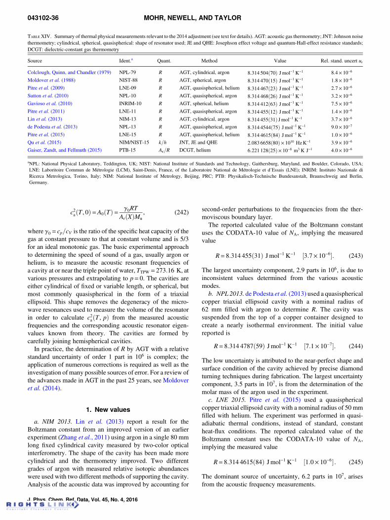
c2aðT , 0Þ=A0ðTÞ= γ0RTArðXÞMu
, (242)
where γ0 = cp=cV is the ratio of the specific heat capacity of thegas at constant pressure to that at constant volume and is 5/3for an ideal monotonic gas. The basic experimental approachto determining the speed of sound of a gas, usually argon orhelium, is to measure the acoustic resonant frequencies ofa cavity at or near the triple point of water, TTPW = 273:16 K, atvarious pressures and extrapolating to p= 0. The cavities areeither cylindrical of fixed or variable length, or spherical, butmost commonly quasispherical in the form of a triaxialellipsoid. This shape removes the degeneracy of the micro-wave resonances used to measure the volume of the resonatorin order to calculate c2aðT , pÞ from the measured acousticfrequencies and the corresponding acoustic resonator eigen-values known from theory. The cavities are formed bycarefully joining hemispherical cavities.
In practice, the determination of R by AGT with a relativestandard uncertainty of order 1 part in 106 is complex; theapplication of numerous corrections is required as well as theinvestigation of many possible sources of error. For a review ofthe advances made in AGT in the past 25 years, see Moldoveret al. (2014).
1. New values
a. NIM 2013. Lin et al. (2013) report a result for theBoltzmann constant from an improved version of an earlierexperiment (Zhang et al., 2011) using argon in a single 80 mmlong fixed cylindrical cavity measured by two-color opticalinterferometry. The shape of the cavity has been made morecylindrical and the thermometry improved. Two differentgrades of argon with measured relative isotopic abundanceswere used with two different methods of supporting the cavity.Analysis of the acoustic data was improved by accounting for
second-order perturbations to the frequencies from the ther-moviscous boundary layer.
The reported calculated value of the Boltzmann constantuses the CODATA-10 value of NA, implying the measuredvalue
R= 8:314 455ð31Þ Jmol−1 K−1 ½3:7× 10⁻⁶�. (243)
The largest uncertainty component, 2.9 parts in 106, is due toinconsistent values determined from the various acousticmodes.
b. NPL 2013. de Podesta et al. (2013) used a quasisphericalcopper triaxial ellipsoid cavity with a nominal radius of62 mm filled with argon to determine R. The cavity wassuspended from the top of a copper container designed tocreate a nearly isothermal environment. The initial valuereported is
R= 8:314 4787ð59Þ Jmol−1 K−1 ½7:1× 10⁻⁷�. (244)
The low uncertainty is attributed to the near-perfect shape andsurface condition of the cavity achieved by precise diamondturning techniques during fabrication. The largest uncertaintycomponent, 3.5 parts in 107, is from the determination of themolar mass of the argon used in the experiment.
c. LNE 2015. Pitre et al. (2015) used a quasisphericalcopper triaxial ellipsoid cavity with a nominal radius of 50 mmfilled with helium. The experiment was performed in quasi-adiabatic thermal conditions, instead of standard, constantheat-flux conditions. The reported calculated value of theBoltzmann constant uses the CODATA-10 value of NA,implying the measured value
R= 8:314 4615ð84Þ Jmol−1 K−1 ½1:0× 10−6� . (245)
The dominant source of uncertainty, 6.2 parts in 107, arisesfrom the acoustic frequency measurements.
TABLE XIV. Summary of thermal physical measurements relevant to the 2014 adjustment (see text for details). AGT: acoustic gas thermometry; JNT: Johnson noisethermometry; cylindrical, spherical, quasispherical: shape of resonator used; JE and QHE: Josephson effect voltage and quantum-Hall-effect resistance standards;DCGT: dielectric-constant gas thermometry
Source Ident.a Quant. Method Value Rel. stand. uncert ur
Colclough, Quinn, and Chandler (1979) NPL-79 R AGT, cylindrical, argon 8:314 504ð70Þ Jmol−1 K−1 8:4× 10⁻⁶
Moldover et al. (1988) NIST-88 R AGT, spherical, argon 8:314 470ð15Þ Jmol−1 K−1 1:8× 10⁻⁶
Pitre et al. (2009) LNE-09 R AGT, quasispherical, helium 8:314 467ð23Þ Jmol−1 K−1 2:7× 10⁻⁶
Sutton et al. (2010) NPL-10 R AGT, quasispherical, argon 8:314 468ð26Þ Jmol−1 K−1 3:2× 10⁻⁶
Gavioso et al. (2010) INRIM-10 R AGT, spherical, helium 8:314 412ð63Þ Jmol−1 K−1 7:5× 10⁻⁶
Pitre et al. (2011) LNE-11 R AGT, quasispherical, argon 8:314 455ð12Þ Jmol−1 K−1 1:4× 10⁻⁶
Lin et al. (2013) NIM-13 R AGT, cylindrical, argon 8:314 455ð31Þ Jmol−1 K−1 3:7× 10⁻⁶
de Podesta et al. (2013) NPL-13 R AGT, quasispherical, argon 8:314 4544ð75Þ Jmol−1 K−1 9:0× 10−7
Pitre et al. (2015) LNE-15 R AGT, quasispherical, helium 8:314 4615ð84Þ Jmol−1 K−1 1:0× 10−6
Qu et al. (2015) NIM/NIST-15 k=h JNT, JE and QHE 2:083 6658ð80Þ× 1010 HzK−1 3:9× 10⁻⁶
Gaiser, Zandt, and Fellmuth (2015) PTB-15 Ae=R DCGT, helium 6:221 128ð25Þ× 10−8 m3 K J−1 4:0× 10−6
aNPL: National Physical Laboratory, Teddington, UK; NIST: National Institute of Standards and Technology, Gaithersburg, Maryland, and Boulder, Colorado, USA;LNE: Laboritoire Commun de Metrologie (LCM), Saint-Denis, France, of the Laboratoire National de Metrologie et d’Essais (LNE); INRIM: Instituto Nazionale diRicerca Metrologica, Torino, Italy; NIM: National Institute of Metrology, Beijing, PRC; PTB: Physikalisch-Technische Bundesanstalt, Braunschweig and Berlin,Germany.
043102-36 MOHR, NEWELL, AND TAYLOR
J. Phys. Chem. Ref. Data, Vol. 45, No. 4, 2016
2. Updated values
The following updates and corrections for the AGT inputdata are summarized in Moldover, Gavioso, and Newell(2015), along with a detailed description of the correlationcoefficients given in Table XIX. The AGT values and un-certainties in Table XIV incorporate all the corrections listedbelow.
a. Molar mass of argon. During the period from October toDecember 2014, three important studies on the molar mass ofargon MðArÞ were performed to investigate the difference of2.74 parts in 106 between the results from LNE-11 and NPL-13(Yang et al., 2015). The LNE-11 value is based on MðArÞdeterminations from the Institute for Reference Materials andMeasurements (IRMM), Geel, Belgium (Valkiers et al., 2010).The NPL-13 estimate ofMðArÞ is based on a comparison at theScottish Universities Environmental Research Centre(SUERC), University of Glasgow, Glasgow, Scotland, of theisotopic composition of the experimental gas with the isotopiccomposition of argon from atmospheric air (de Podesta et al.,2013), assuming the atmospheric air had the same argonisotopic abundance as the analysis performed by Lee et al.(2006) at the Korea Research Institute of Standards andScience (KRISS), Taedoc Science Town, Republic of Korea.The results of these studies were discussed at the meeting of theCIPM Consultative Committee for Thermometry Task Groupfor the SI (CCT TG-SI) in Eltville, Germany, on 6 February2015 in conjunction with the 2015 Fundamental ConstantsMeeting co-organized by the Task Group (Karshenboim,Mohr, and Newell, 2015).
In the first study, the isotopic composition of samples ofargon gas previously measured at the IRMMwere remeasured.The analysis showed disagreements in values of MðArÞ of upto 3.5 parts in 106. In the second study, the isotopiccomposition of a sample of argon gas used for isotherm 5 ofNPL-13 was remeasured. The estimate of MðArÞ was 2.73parts in 106 lower than the corresponding SUERC estimate. Inthe third study, mass spectrometry measurements were madeon a series of argon samples from NIM, INRIM, NPL, NMIJand LNE on which corresponding speed-of-sound measure-ments had been made at LNE. The results showed the expectedcorrelation between the two sets of measurements. From thisstudy an inference of the required correction to the SUERCestimate of the NPL-13 isotherm 5 molar mass of −3:6 parts in106 was apparent. However, KRISS considered their directmeasurement of this sample to have a lower uncertainty. Theinference of the required correction to the LNE-11MðArÞ wasnot strong enough to suggest a meaningful change in its value.
Although the estimated relative statistical uncertainty for theKRISS MðArÞ measurements was 0:61× 10−6, KRISS con-sidered it likely that the isotope ratio Rð38Ar=36ArÞ may be inerror because it disagrees distinctly with measurements fromLee et al. (2006). For this reason an additional relativeuncertainty of 0:35× 10−6 was added in quadrature to yieldan overall relative uncertainty for the KRISS MðArÞ measure-ments of 0:7× 10⁻⁶.
Based on the studies at KRISS it was agreed upon by allparticipants of the CCT TG-SI meeting that for the 2014
CODATA adjustment, the NPL-13 determination of the molargas constant will rely on the KRISS value and uncertainty ofMðArÞ, resulting in a fractional correction of −2:73× 10−6 anda total relative uncertainty of 0:9× 10⁻⁶ (de Podesta et al.,2015). It was also agreed that while the LNE-11 value of themolar gas constant will continue to use the determinationof MðArÞ from IRMM, the relative uncertainty will be thatof KRISS, namely 0:7× 10⁻⁶. Similarly since the previousNPL-10 result used the MðArÞ value from IRMM, the relativeuncertainty component for MðArÞ for NPL-10 was increasedto 0:7× 10⁻⁶.
b. Molar mass of helium. Based upon the measured3He=4He abundance ratios spanning 0:05× 10−6 to0:5× 10⁻⁶ from samples taken from 12 natural gas wells inthe USA (Aldrich and Nier, 1948), the expected reduction inMð4HeÞ due to naturally occurring 3He is fractionally from0:012× 10−6 to 0:12× 10−6. The two gas analyses given in thepaper by Gavioso et al. (2015) are consistent with thisexpectation (see Sec. X.D). In contrast, the ratio of speed-of-sound measurements using two different, commercially pro-duced, highly purified helium samples given in the paperreporting LNE-15 differed by the surprisingly large value of0.44 parts in 106. This observation was taken into account byincluding an additional uncertainty component of 0.5 parts in106. Based upon the possibility that the concentration of 3Hemay be higher than expected, an additional relative uncertaintycomponent of 0:5× 10⁻⁶ was incorporated in the LNE-09result. It should finally be noted that certain natural gases inTaiwan have 3He/4He abundance ratios as large as 3:8× 10⁻⁶
(Sano, Wakita, and Huang, 1986). Clearly, future helium-based low-uncertainty AGT determinations of Rmust measurethe 3He concentration in the gas samples used.
c. Thermal conductivity of argon. An improved estimatefor the thermal conductivity of argon became available forthe 2014 CODATA adjustment [see supplementary data inMoldover et al. (2014)]. A change in thermal conductivityaffects the estimate for the thermal boundary layer thicknessclose to the wall of the cavity, resulting in a correction for allresonant frequencies at all pressures. For the 2014 CODATAadjustment, these corrections are applied to the lowestuncertainty results for AGT using argon. In parts in 106, thecorrections to NIST-88 (Moldover, 2015), LNE-11 (Pitre,2015), and NPL-13 (de Podesta et al., 2015) are −0:16,−0:16, and −0:192, respectively, with inconsequential de-creases in the uncertainties.
B. Quotient k/h, Johnson noise thermometry
The Nyquist theorem predicts that, with a fractional error ofless than 1 part in 106 at frequencies less than 10 MHz andtemperatures greater than 250 K,
ÆU2æ= 4kTRsΔf . (246)
Here ÆU2æ is the mean-square voltage, or Johnson noisevoltage, in a measurement bandwidth of frequency Δf acrossthe terminals of a resistor of resistance Rs in thermal equili-brium at thermodynamic temperature T . If ÆU2æ is measured in
CODATA RECOMMENDED VALUES: 2014 043102-37
J. Phys. Chem. Ref. Data, Vol. 45, No. 4, 2016
terms of the Josephson constant KJ = 2e=h and Rs in terms ofthe von Klitzing constant RK = h=e2, then the measurementyields a value of k=h.
Continuing the pioneering work of Benz et al. (2011), Quet al. (2015) report an improved determination of the Boltzmannconstant using such a method. The reported value is
k90 = 1:380 6513ð53Þ× 10−23 J K−1 ½3:9× 10⁻⁶� , (247)
where k90 in the SI unit J/K is the result of a Johnson noiseexperiment when the voltage and resistance are measured inconventional electrical units defined by KJ−90 and RK−90.Following the analysis given in CODATA-98 [see Eqs.(29d) and (317)], it can be shown that k90=h90 = k=h. Usingthe value of h90 (see the introduction to Sec. VIII), themeasured value of k=h is
k=h= 2:083 6658ð80Þ× 1010 HzK−1 ½3:9× 10⁻⁶� , (248)
as given in Table XIV.In the Qu et al. (2015) experiment, digitally synthesized
pseudonoise voltages VQ are generated by means of a pulse-biased Josephson junction array. These known voltages arecompared to the unknown thermal-noise voltages VR generatedby a specially designed 200 Ω resistor in a well regulatedthermal cell at or near TTPW. Since the spectral density of thenoise voltage of a 200 Ω resistor at 273.16 K is only1:74 nV
ffiffiffiffiffiffiHz
p, it is measured using a low-noise, two-channel,
cross-correlation technique that enables the resistor signal to beextracted from uncorrelated amplifier noise of comparableamplitude and spectral density. The final result is based onmeasurements integrated over a bandwidth of 575 kHz anda total integration time of about 33 d.
The dominant uncertainty contributions of 3.2 parts in 106
and 1.8 parts in 106 are from the statistical uncertainty of theÆV2
R=V2Qæ ratio measurement and the ambiguity associated with
the spectral mismatch model, respectively.
C. Quotient Ae/R, dielectric-constantgas thermometry
The virial expansion of the equation of state for a real gas ofamount of substance n in a volume V is
p= ρRT ½1+ ρBðTÞ+ ρ2CðTÞ+ ρ3DðTÞ+⋯� , (249)
where ρ= n=V is the amount-of-substance density of the gas atthermodynamic temperature T , and BðTÞ, CðTÞ, etc. are thevirial coefficients. The Clausius-Mossotti equation is
er − 1er + 2
= ρAe½1+ ρBeðTÞ+ ρ2CeðTÞ+ ρ3DeðTÞ+⋯� , (250)
where er = e=e0 is the relative dielectric constant (relativepermittivity) of the gas, e is its dielectric constant, e0 is theexactly known electric constant, Ae is the molar polarizabilityof the atoms, and BeðTÞ, CeðTÞ, etc., are the dielectric virialcoefficients. By appropriately combining Eqs. (249) and (250),
an expression is obtained from which Ae=R can be experi-mentally determined by measuring er at a known constanttemperature such as TTPW and at different pressures andextrapolating to zero pressure.
In practice, dielectric-constant gas thermometry measuresthe fractional change in capacitance of a specially constructedcapacitor, first without helium gas and then with helium gasat a known pressure. The static electric polarizability of a gasatom α0, Ae, R, and k are related by Ae=R=α0=3e0k, whichshows that if α0 is known sufficiently well from theory, thena competitive value of k can be obtained if the quotient Ae=Rcan be measured with a sufficiently small uncertainty.
Piszczatowski et al. (2015) have calculated the static electricpolarizability of 4He in atomic units to be
α*0ð4HeÞ= 1:383 760 77ð14Þ a. u. ½1:0× 10−7� , (251)
from which the static electric polarizability of 4He in SI units is
α0ð4HeÞ= 4πe0a30α
*0ð4HeÞ , (252)
where a0 and e0 are the Bohr radius and electric constant,respectively.
Superseding previous preliminary results (Fellmuth et al.,2011; Gaiser and Fellmuth, 2012), Gaiser et al. (2013) reporta final value of Ae=R from dielectric-constant gas thermometrywith an updated uncertainty given by Gaiser, Zandt, andFellmuth (2015):
Ae=R= 6:221 128ð25Þ× 10−8 m3 K J−1 ½4:0× 10−6� . (253)
The dominant uncertainty components are the fitted coefficientfrom the 10 isotherms (statistical) and the effective compress-ibility of the capacitor assembly at 2.6 parts in 106 and 2.4 partsin 106, respectively.
D. Other data
For completeness we note the following result that becameavailable only after the 31 December 2014 closing date of the2014 adjustment. Gavioso et al. (2015) obtained the very com-petitive value R= 8:314 4743ð88Þ Jmol−1 K−1½1:06× 10−6�using acoustic gas thermometry with a misaligned sphericalcavity with a nominal radius of 90 mm filled with helium.This value is 1.47 parts in 106 larger than the 2014 CODATAvalue.
E. Stefan-Boltzmann constant σ
The Stefan-Boltzmann constant is related to c, h, and kby σ= 2π5k4=15h3c2, which, with the aid of the relationsk =R=NA and NAh= cArðeÞMuα
2=2R∞, can be expressed interms of the molar gas constant and other adjusted constantsas
σ=32π5h15c6
R∞R
ArðeÞMuα2
�4
. (254)
043102-38 MOHR, NEWELL, AND TAYLOR
J. Phys. Chem. Ref. Data, Vol. 45, No. 4, 2016
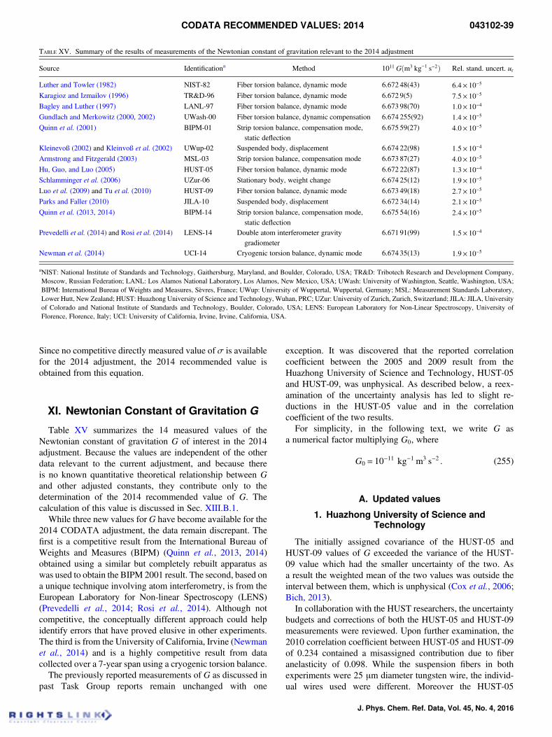
Since no competitive directly measured value of σ is availablefor the 2014 adjustment, the 2014 recommended value isobtained from this equation.
XI. Newtonian Constant of Gravitation G
Table XV summarizes the 14 measured values of theNewtonian constant of gravitation G of interest in the 2014adjustment. Because the values are independent of the otherdata relevant to the current adjustment, and because thereis no known quantitative theoretical relationship between Gand other adjusted constants, they contribute only to thedetermination of the 2014 recommended value of G. Thecalculation of this value is discussed in Sec. XIII.B.1.
While three new values for G have become available for the2014 CODATA adjustment, the data remain discrepant. Thefirst is a competitive result from the International Bureau ofWeights and Measures (BIPM) (Quinn et al., 2013, 2014)obtained using a similar but completely rebuilt apparatus aswas used to obtain the BIPM 2001 result. The second, based ona unique technique involving atom interferometry, is from theEuropean Laboratory for Non-linear Spectroscopy (LENS)(Prevedelli et al., 2014; Rosi et al., 2014). Although notcompetitive, the conceptually different approach could helpidentify errors that have proved elusive in other experiments.The third is from the University of California, Irvine (Newmanet al., 2014) and is a highly competitive result from datacollected over a 7-year span using a cryogenic torsion balance.
The previously reported measurements of G as discussed inpast Task Group reports remain unchanged with one
exception. It was discovered that the reported correlationcoefficient between the 2005 and 2009 result from theHuazhong University of Science and Technology, HUST-05and HUST-09, was unphysical. As described below, a reex-amination of the uncertainty analysis has led to slight re-ductions in the HUST-05 value and in the correlationcoefficient of the two results.
For simplicity, in the following text, we write G asa numerical factor multiplying G0, where
G0 = 10−11 kg−1 m3 s−2 . (255)
A. Updated values
1. Huazhong University of Science andTechnology
The initially assigned covariance of the HUST-05 andHUST-09 values of G exceeded the variance of the HUST-09 value which had the smaller uncertainty of the two. Asa result the weighted mean of the two values was outside theinterval between them, which is unphysical (Cox et al., 2006;Bich, 2013).
In collaboration with the HUST researchers, the uncertaintybudgets and corrections of both the HUST-05 and HUST-09measurements were reviewed. Upon further examination, the2010 correlation coefficient between HUST-05 and HUST-09of 0.234 contained a misassigned contribution due to fiberanelasticity of 0.098. While the suspension fibers in bothexperiments were 25 μm diameter tungsten wire, the individ-ual wires used were different. Moreover the HUST-05
TABLE XV. Summary of the results of measurements of the Newtonian constant of gravitation relevant to the 2014 adjustment
Source Identificationa Method 1011 Gðm3 kg−1 s−2Þ Rel. stand. uncert. ur
Luther and Towler (1982) NIST-82 Fiber torsion balance, dynamic mode 6.672 48(43) 6:4× 10⁻⁵
Karagioz and Izmailov (1996) TR&D-96 Fiber torsion balance, dynamic mode 6.672 9(5) 7:5× 10⁻⁵
Bagley and Luther (1997) LANL-97 Fiber torsion balance, dynamic mode 6.673 98(70) 1:0× 10−4
Gundlach and Merkowitz (2000, 2002) UWash-00 Fiber torsion balance, dynamic compensation 6.674 255(92) 1:4× 10⁻⁵
Quinn et al. (2001) BIPM-01 Strip torsion balance, compensation mode,static deflection
6.675 59(27) 4:0× 10−5
Kleinevoß (2002) and Kleinvoß et al. (2002) UWup-02 Suspended body, displacement 6.674 22(98) 1:5× 10⁻⁴
Armstrong and Fitzgerald (2003) MSL-03 Strip torsion balance, compensation mode 6.673 87(27) 4:0× 10−5
Hu, Guo, and Luo (2005) HUST-05 Fiber torsion balance, dynamic mode 6.672 22(87) 1:3× 10⁻⁴
Schlamminger et al. (2006) UZur-06 Stationary body, weight change 6.674 25(12) 1:9× 10⁻⁵
Luo et al. (2009) and Tu et al. (2010) HUST-09 Fiber torsion balance, dynamic mode 6.673 49(18) 2:7× 10⁻⁵
Parks and Faller (2010) JILA-10 Suspended body, displacement 6.672 34(14) 2:1× 10⁻⁵
Quinn et al. (2013, 2014) BIPM-14 Strip torsion balance, compensation mode,static deflection
6.675 54(16) 2:4× 10⁻⁵
Prevedelli et al. (2014) and Rosi et al. (2014) LENS-14 Double atom interferometer gravitygradiometer
6.671 91(99) 1:5× 10⁻⁴
Newman et al. (2014) UCI-14 Cryogenic torsion balance, dynamic mode 6.674 35(13) 1:9× 10⁻⁵
aNIST: National Institute of Standards and Technology, Gaithersburg, Maryland, and Boulder, Colorado, USA; TR&D: Tribotech Research and Development Company,Moscow, Russian Federation; LANL: Los Alamos National Laboratory, Los Alamos, New Mexico, USA; UWash: University of Washington, Seattle, Washington, USA;BIPM: International Bureau of Weights and Measures, Sevres, France; UWup: University of Wuppertal, Wuppertal, Germany; MSL: Measurement Standards Laboratory,Lower Hutt, New Zealand; HUST: Huazhong University of Science and Technology, Wuhan, PRC; UZur: University of Zurich, Zurich, Switzerland; JILA: JILA, Universityof Colorado and National Institute of Standards and Technology, Boulder, Colorado, USA; LENS: European Laboratory for Non-Linear Spectroscopy, University ofFlorence, Florence, Italy; UCI: University of California, Irvine, Irvine, California, USA.
CODATA RECOMMENDED VALUES: 2014 043102-39
J. Phys. Chem. Ref. Data, Vol. 45, No. 4, 2016
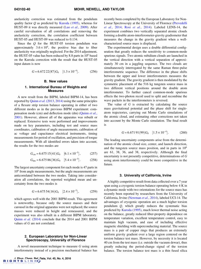
anelasticity correction was estimated from the pendulumquality factor Q as predicted by Kuroda (1995), whereas forHUST-09 it was directly measured (Luo et al., 2009). Aftercareful reevaluation of all correlations and removing theanelasticity correction, the correlation coefficient betweenHUST-05 and HUST-09 was reduced to 0.134.
Since the Q for the HUST-05 torsion pendulum wasapproximately 3:6× 10⁴, the positive bias due to fiberanelasticity was originally neglected. For the 2014 adjustment,the HUST-05 value has been reduced by 8.8 parts in 106 basedon the Kuroda correction with the result that the HUST-05input datum is now
G= 6:672 22ð87ÞG0 ½1:3× 10⁻⁴� . (256)
B. New values
1. International Bureau of Weights andMeasures
A new result from the BIPM, labeled BIPM-14, has beenreported by Quinn et al. (2013, 2014) using the same principlesof a flexure strip torsion balance operating in either of twodifferent modes as in the previous BIPM experiment: com-pensation mode (cm) and deflection mode (dm) (Quinn et al.,2001). However, almost all of the apparatus was rebuilt orreplaced. Extensive tests were performed and improvementsmade on key parameters, including test and source masscoordinates, calibration of angle measurements, calibration ofac voltage and capacitance electrical instruments, timingmeasurements for period of oscillation, and precision of torquemeasurements. With all identified errors taken into account,the results for the two modes are
Gcm = 6:675 15ð41ÞG0 ½6:1× 10⁻⁵� , (257)
Gdm = 6:675 86ð36ÞG0 ½5:4× 10⁻⁵� . (258)
The largest uncertainty component for each mode is 47 parts in106 from angle measurements, but the angle measurements areanticorrelated between the two modes. Taking into consider-ation all correlations, the reported weighted mean and un-certainty from the two modes is
G= 6:675 54ð16ÞG0 ½2:4× 10⁻⁵� , (259)
which agrees well with the 2001 BIPM result. This agreementis noteworthy, because only the source masses and theircarousel in the original apparatus were not replaced; the sourcemasses were reduced in height and remeasured, and theexperiment was also rebuilt in a different BIPM laboratory.Quinn et al. (2014) conclude that the 2014 and 2001 BIPMvalues of G are not correlated.
2. European Laboratory for Non-LinearSpectroscopy, University of Florence
A novel measurement technique to measure G using atominterferometry instead of a precision mechanical balance has
recently been completed by the European Laboratory for Non-Linear Spectroscopy at the University of Florence (Prevedelliet al., 2014; Rosi et al., 2014). Labeled LENS-14, theexperiment combines two vertically separated atomic cloudsforming a double atom-interferometer-gravity gradiometer thatmeasures the change in the gravity gradient when a well-characterized source mass is displaced.
The experimental design uses a double differential config-uration that greatly reduces the sensitivity to common-modespurious signals. Two atomic rubidium clouds are launched inthe vertical direction with a vertical separation of approxi-mately 30 cm in a juggling sequence. The two clouds aresimultaneously interrogated by the same Raman three-pulseinterferometric sequence. The difference in the phase shiftsbetween the upper and lower interferometers measures thegravity gradient. The gravity gradient is then modulated by thesymmetric placement of the 516 kg tungsten source mass intwo different vertical positions around the double atominterferometer. To further cancel common-mode spuriouseffects the two-photon recoil used to split and recombine thewave packets in the interferometers is reversed.
The value of G is extracted by calculating the sourcemass gravitational potential and the phase shift for single-atom trajectories, carrying out Monte Carlo simulations ofthe atomic cloud, and estimating other corrections not takeninto account by the Monte Carlo simulation. The final resultis
G= 6:671 91ð99ÞG0 ½1:5× 10⁻⁴� . (260)
The leading uncertainty components arise from the determi-nation of the atomic cloud size, center, and launch direction,and the tungsten source mass position, and in parts in 106
are 61, 38, 36, and 38, respectively. Although the finaluncertainty is not presently competitive, determinations of Gusing atom interferometry could be more competitive in thefuture.
3. University of California, Irvine
A highly competitive result from data collected over a 7 yearspan using a cryogenic torsion balance operating below 4 K ina dynamic mode with two orientations for the source mass hasrecently been reported by researchers from the University ofCalifornia, Irvine (Newman et al., 2014), labeled UCI-14. Theadvantages of cryogenic operation are a much higher torsionpendulum Q, which greatly reduces the systematic biaspredicted by Kuroda (1995), much lower thermal noise actingon the balance, greatly reduced fiber-property dependence ontemperature variation, excellent temperature control, easy tomaintain high vacuum, and ease of including effectivemagnetic shielding with superconducting material. The sourcemass is a pair of copper rings that produces an extremelyuniform gravity gradient over a large region centered on thetorsion balance test mass. However, by necessity it is located40 cm from the test mass (i.e. outside the vacuum dewar), thusgreatly reducing the period-change signal of the torsionbalance. The torsion balance test mass is a thin fused silica
043102-40 MOHR, NEWELL, AND TAYLOR
J. Phys. Chem. Ref. Data, Vol. 45, No. 4, 2016
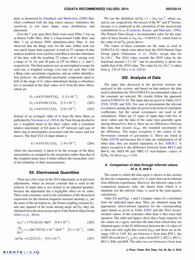
plate as pioneered by Gundlach and Merkowitz (2000) that,when combined with the ring source masses, minimizes thesensitivity to test mass shape, mass distribution, andplacement.
Over the 7 year span three fibers were used. Fiber 1 was anas-drawn CuBe fiber, fiber 2 a heat-treated CuBe fiber, andfiber 3 an as-drawn 5056 aluminium-alloy fiber. It wasobserved that the Birge ratio for the data within each runwas much larger than expected. A total of 27 variants of dataanalysis methods were used for each fiber to test the robustnessof the data, with the resulting 27 values of G varying overa range of 14, 24, and 20 parts in 106 for fibers 1, 2, and 3,respectively. The final analysis uses an unweighted average foreach run, a weighted average over runs for each fiber witha Birge ratio uncertainty expansion, and an outlier identifica-tion protocol. An additional uncertainty component equal tohalf of the range of G values determined during a robustnesstest is included in the final values of G from the three fibers,which are
G1 = 6:674 350ð97ÞG0 ½1:5× 10⁻⁵� , (261)
G2 = 6:674 08ð15ÞG0 ½2:2× 10⁻⁵� , (262)
G3 = 6:674 55ð13ÞG0 ½2:0× 10−5� . (263)
Instead of an averaged value of G from the three fibers aspublished by Newman et al. (2014), the Task Group decided touse a weighted mean of the three values with a correlatedrelative uncertainty of 8.6 parts in 106 between each pair offibers due to uncertainties associated with the source and testmasses. The final UCI-14 input datum is
G= 6:674 35ð13ÞG0 ½1:9× 10⁻⁵� , (264)
where the uncertainty is taken to be the average of the threeuncertainties as assigned by the researchers rather than that ofthe weighted mean since it better reflects the researchers viewof the reliability of their measurements.
XII. Electroweak Quantities
There are a few cases in the 2014 adjustment, as in previousadjustments, where an inexact constant that is used in theanalysis of input data is not treated as an adjusted quantity,because the adjustment has a negligible effect on its value.Three such constants, used in the calculation of the theoreticalexpression for the electron magnetic-moment anomaly ae, arethe mass of the tau lepton mτ, the Fermi coupling constant GF,and sine squared of the weak mixing angle sin2θW; they areobtained from the most recent report of the Particle Data Group(Olive et al., 2014):
mτc2 = 1776:82ð16Þ MeV ½9:0× 10−5� , (265)
GF
ðℏcÞ3 = 1:166 3787ð6Þ× 10−5 GeV−2 ½5:1× 10⁻⁷� , (266)
sin2θW = 0:2223ð21Þ ½9:5× 10⁻³� . (267)
We use the definition sin2θW = 1− ðmW=mZÞ2, where mW
and mZ are, respectively, the masses of the W± and Z0 bosons,because it is employed in the calculation of the electroweakcontributions to ae (Czarnecki, Krause, and Marciano, 1996).The Particle Data Group’s recommended value for the massratio of these bosons is mW=mZ = 0:8819ð12Þ, which leads tothe value of sin2θW given above.
The values of these constants are the same as used inCODATA-10, which were taken from the 2010 Particle DataGroup report (Nakamura et al., 2010), except that forGF=ðℏcÞ3. The 2014 value exceeds the 2010 value by thefractional amount 1:3× 10⁻⁵ and its uncertainty is about oneeighth that of the 2010 value. The value for GF=ðℏcÞ3 is takenfrom p. 139 of Olive et al. (2014).
XIII. Analysis of Data
The input data discussed in the previous sections areanalyzed in this section, and based on that analysis the dataused to determine the 2014 CODATA recommended values ofthe constants are selected. We closely follow the approachused in CODATA-10. The input data are given in Tables XVI,XVII, XVIII, and XIX. For ease of presentation the relevantcovariances among the data are given in the form of correlationcoefficients, but the actual covariances are used in allcalculations. There are 15 types of input data with two ormore values and the data of the same type generally agreeamong themselves; that is, there are no differences betweenlike data that exceed 2udiff , the standard uncertainty ofthe difference. The major exception is the values of theNewtonian constant of gravitation G. These are listed inTable XXVII and because the G data are independent of allother data, they are treated separately in Sec. XIII.B.1. Aminor exception is the difference between items B44:2 andB44:6, the NIST-98 and NRC-15 watt-balance values ofK2
J RK; for these udiff = 2:04.
A. Comparison of data through inferred valuesof α, h, and k
The extent to which the data agree is shown in this sectionby directly comparing values of α, h, and k that can be inferredfrom different experiments. However, the inferred value is forcomparison purposes only; the datum from which it isobtained, not the inferred value, is used in the least-squarescalculations.
Table XX and Figs. 1 and 2 compare values of α calculatedfrom the indicated input data. They are obtained using theappropriate observational equation for the correspondinginput datum as given in Table XXIV and the 2014 recom-mended values of the constants other than α that enter thatequation. The table and figures show that a large majority ofthe values of α agree, and thus the data from which they areobtained agree; of the 91 differences between the 14 values ofα, there are only eight that exceed 2udiff and these are in therange 2.02 to 2.60. Six are between α from item B39:1, theNIST-89 result for Γ0
p−90ðloÞ, and α from B22:1, B22:2, B43:1,B43:3, B46, and B48. The other two are between α from item
CODATA RECOMMENDED VALUES: 2014 043102-41
J. Phys. Chem. Ref. Data, Vol. 45, No. 4, 2016
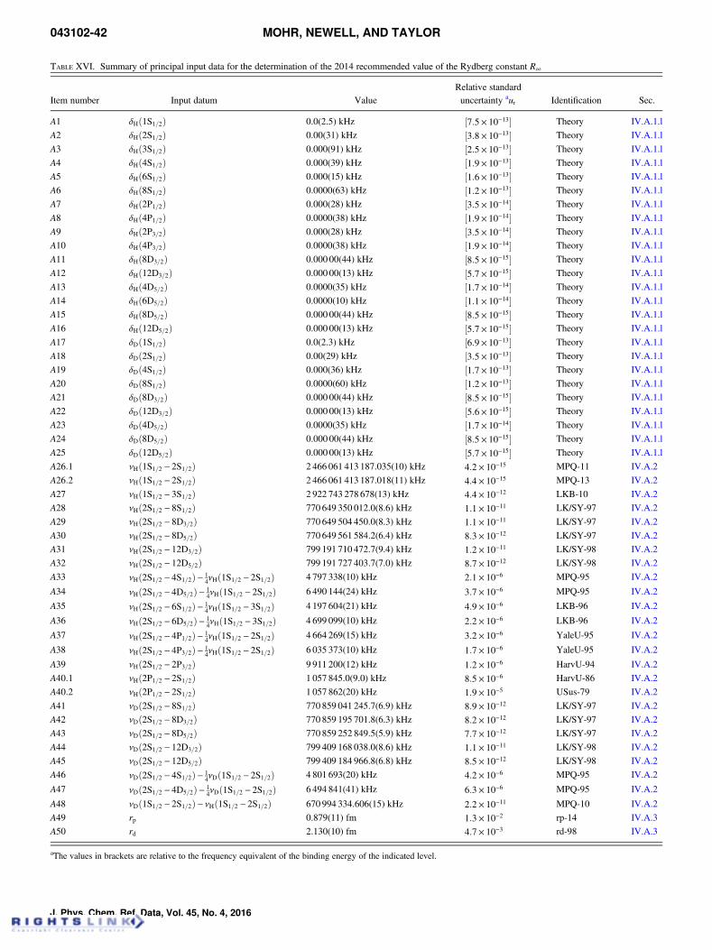
TABLE XVI. Summary of principal input data for the determination of the 2014 recommended value of the Rydberg constant R∞
Item number Input datum ValueRelative standarduncertainty aur Identification Sec.
A1 δHð1S1=2Þ 0.0(2.5) kHz ½7:5× 10⁻¹³� Theory IV.A.1.l
A2 δHð2S1=2Þ 0.00(31) kHz ½3:8× 10⁻¹³� Theory IV.A.1.l
A3 δHð3S1=2Þ 0.000(91) kHz ½2:5× 10⁻¹³� Theory IV.A.1.l
A4 δHð4S1=2Þ 0.000(39) kHz ½1:9× 10⁻¹³� Theory IV.A.1.l
A5 δHð6S1=2Þ 0.000(15) kHz ½1:6× 10⁻¹³� Theory IV.A.1.l
A6 δHð8S1=2Þ 0.0000(63) kHz ½1:2× 10⁻¹³� Theory IV.A.1.l
A7 δHð2P1=2Þ 0.000(28) kHz ½3:5× 10⁻¹⁴� Theory IV.A.1.l
A8 δHð4P1=2Þ 0.0000(38) kHz ½1:9× 10⁻¹⁴� Theory IV.A.1.l
A9 δHð2P3=2Þ 0.000(28) kHz ½3:5× 10⁻¹⁴� Theory IV.A.1.l
A10 δHð4P3=2Þ 0.0000(38) kHz ½1:9× 10⁻¹⁴� Theory IV.A.1.l
A11 δHð8D3=2Þ 0.000 00(44) kHz ½8:5× 10⁻¹⁵� Theory IV.A.1.l
A12 δHð12D3=2Þ 0.000 00(13) kHz ½5:7× 10⁻¹⁵� Theory IV.A.1.l
A13 δHð4D5=2Þ 0.0000(35) kHz ½1:7× 10⁻¹⁴� Theory IV.A.1.l
A14 δHð6D5=2Þ 0.0000(10) kHz ½1:1× 10⁻¹⁴� Theory IV.A.1.l
A15 δHð8D5=2Þ 0.000 00(44) kHz ½8:5× 10⁻¹⁵� Theory IV.A.1.l
A16 δHð12D5=2Þ 0.000 00(13) kHz ½5:7× 10⁻¹⁵� Theory IV.A.1.l
A17 δDð1S1=2Þ 0.0(2.3) kHz ½6:9× 10⁻¹³� Theory IV.A.1.l
A18 δDð2S1=2Þ 0.00(29) kHz ½3:5× 10⁻¹³� Theory IV.A.1.l
A19 δDð4S1=2Þ 0.000(36) kHz ½1:7× 10⁻¹³� Theory IV.A.1.l
A20 δDð8S1=2Þ 0.0000(60) kHz ½1:2× 10⁻¹³� Theory IV.A.1.l
A21 δDð8D3=2Þ 0.000 00(44) kHz ½8:5× 10⁻¹⁵� Theory IV.A.1.l
A22 δDð12D3=2Þ 0.000 00(13) kHz ½5:6× 10⁻¹⁵� Theory IV.A.1.l
A23 δDð4D5=2Þ 0.0000(35) kHz ½1:7× 10⁻¹⁴� Theory IV.A.1.l
A24 δDð8D5=2Þ 0.000 00(44) kHz ½8:5× 10⁻¹⁵� Theory IV.A.1.l
A25 δDð12D5=2Þ 0.000 00(13) kHz ½5:7× 10⁻¹⁵� Theory IV.A.1.l
A26:1 νHð1S1=2 − 2S1=2Þ 2 466 061 413 187.035(10) kHz 4:2× 10⁻¹⁵ MPQ-11 IV.A.2
A26:2 νHð1S1=2 − 2S1=2Þ 2 466 061 413 187.018(11) kHz 4:4× 10⁻¹⁵ MPQ-13 IV.A.2
A27 νHð1S1=2 − 3S1=2Þ 2 922 743 278 678(13) kHz 4:4× 10⁻¹² LKB-10 IV.A.2
A28 νHð2S1=2 − 8S1=2Þ 770 649 350 012.0(8.6) kHz 1:1× 10⁻¹¹ LK/SY-97 IV.A.2
A29 νHð2S1=2 − 8D3=2Þ 770 649 504 450.0(8.3) kHz 1:1× 10⁻¹¹ LK/SY-97 IV.A.2
A30 νHð2S1=2 − 8D5=2Þ 770 649 561 584.2(6.4) kHz 8:3× 10⁻¹² LK/SY-97 IV.A.2
A31 νHð2S1=2 − 12D3=2Þ 799 191 710 472.7(9.4) kHz 1:2× 10⁻¹¹ LK/SY-98 IV.A.2
A32 νHð2S1=2 − 12D5=2Þ 799 191 727 403.7(7.0) kHz 8:7× 10⁻¹² LK/SY-98 IV.A.2
A33 νHð2S1=2 − 4S1=2Þ− 14νHð1S1=2 − 2S1=2Þ 4 797 338(10) kHz 2:1× 10⁻⁶ MPQ-95 IV.A.2
A34 νHð2S1=2 − 4D5=2Þ− 14νHð1S1=2 − 2S1=2Þ 6 490 144(24) kHz 3:7× 10⁻⁶ MPQ-95 IV.A.2
A35 νHð2S1=2 − 6S1=2Þ− 14νHð1S1=2 − 3S1=2Þ 4 197 604(21) kHz 4:9× 10⁻⁶ LKB-96 IV.A.2
A36 νHð2S1=2 − 6D5=2Þ− 14νHð1S1=2 − 3S1=2Þ 4 699 099(10) kHz 2:2× 10⁻⁶ LKB-96 IV.A.2
A37 νHð2S1=2 − 4P1=2Þ− 14νHð1S1=2 − 2S1=2Þ 4 664 269(15) kHz 3:2× 10⁻⁶ YaleU-95 IV.A.2
A38 νHð2S1=2 − 4P3=2Þ− 14νHð1S1=2 − 2S1=2Þ 6 035 373(10) kHz 1:7× 10⁻⁶ YaleU-95 IV.A.2
A39 νHð2S1=2 − 2P3=2Þ 9 911 200(12) kHz 1:2× 10⁻⁶ HarvU-94 IV.A.2
A40:1 νHð2P1=2 − 2S1=2Þ 1 057 845.0(9.0) kHz 8:5× 10⁻⁶ HarvU-86 IV.A.2
A40:2 νHð2P1=2 − 2S1=2Þ 1 057 862(20) kHz 1:9× 10⁻⁵ USus-79 IV.A.2
A41 νDð2S1=2 − 8S1=2Þ 770 859 041 245.7(6.9) kHz 8:9× 10⁻¹² LK/SY-97 IV.A.2
A42 νDð2S1=2 − 8D3=2Þ 770 859 195 701.8(6.3) kHz 8:2× 10⁻¹² LK/SY-97 IV.A.2
A43 νDð2S1=2 − 8D5=2Þ 770 859 252 849.5(5.9) kHz 7:7× 10⁻¹² LK/SY-97 IV.A.2
A44 νDð2S1=2 − 12D3=2Þ 799 409 168 038.0(8.6) kHz 1:1× 10⁻¹¹ LK/SY-98 IV.A.2
A45 νDð2S1=2 − 12D5=2Þ 799 409 184 966.8(6.8) kHz 8:5× 10⁻¹² LK/SY-98 IV.A.2
A46 νDð2S1=2 − 4S1=2Þ− 14νDð1S1=2 − 2S1=2Þ 4 801 693(20) kHz 4:2× 10⁻⁶ MPQ-95 IV.A.2
A47 νDð2S1=2 − 4D5=2Þ− 14νDð1S1=2 − 2S1=2Þ 6 494 841(41) kHz 6:3× 10⁻⁶ MPQ-95 IV.A.2
A48 νDð1S1=2 − 2S1=2Þ− νHð1S1=2 − 2S1=2Þ 670 994 334.606(15) kHz 2:2× 10⁻¹¹ MPQ-10 IV.A.2
A49 rp 0.879(11) fm 1:3× 10⁻² rp-14 IV.A.3
A50 rd 2.130(10) fm 4:7× 10⁻³ rd-98 IV.A.3
aThe values in brackets are relative to the frequency equivalent of the binding energy of the indicated level.
043102-42 MOHR, NEWELL, AND TAYLOR
J. Phys. Chem. Ref. Data, Vol. 45, No. 4, 2016
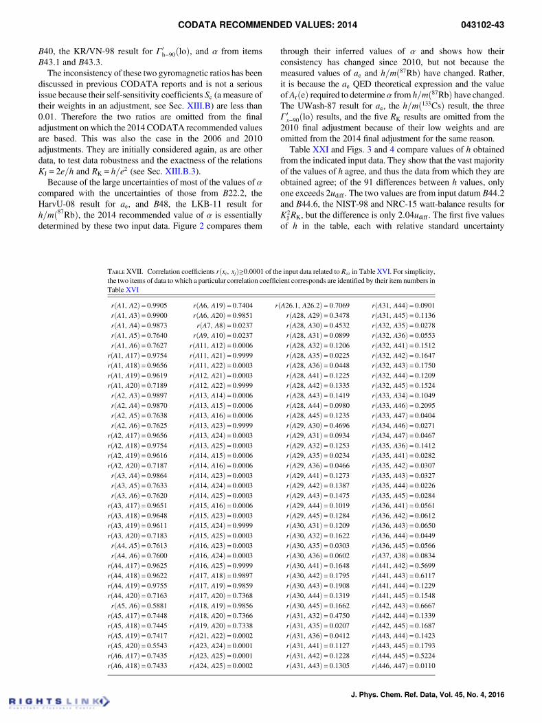
B40, the KR/VN-98 result for Γ0h−90ðloÞ, and α from items
B43:1 and B43:3.The inconsistency of these two gyromagnetic ratios has been
discussed in previous CODATA reports and is not a seriousissue because their self-sensitivity coefficients Sc (a measure oftheir weights in an adjustment, see Sec. XIII.B) are less than0.01. Therefore the two ratios are omitted from the finaladjustment on which the 2014 CODATA recommended valuesare based. This was also the case in the 2006 and 2010adjustments. They are initially considered again, as are otherdata, to test data robustness and the exactness of the relationsKJ = 2e=h and RK = h=e2 (see Sec. XIII.B.3).
Because of the large uncertainties of most of the values of αcompared with the uncertainties of those from B22:2, theHarvU-08 result for ae, and B48, the LKB-11 result forh=mð87RbÞ, the 2014 recommended value of α is essentiallydetermined by these two input data. Figure 2 compares them
through their inferred values of α and shows how theirconsistency has changed since 2010, but not because themeasured values of ae and h=mð87RbÞ have changed. Rather,it is because the ae QED theoretical expression and the valueofArðeÞ required to determine α from h=mð87RbÞ have changed.The UWash-87 result for ae, the h=mð133CsÞ result, the threeΓ0x−90ðloÞ results, and the five RK results are omitted from the
2010 final adjustment because of their low weights and areomitted from the 2014 final adjustment for the same reason.
Table XXI and Figs. 3 and 4 compare values of h obtainedfrom the indicated input data. They show that the vast majorityof the values of h agree, and thus the data from which they areobtained agree; of the 91 differences between h values, onlyone exceeds 2udiff . The two values are from input datum B44:2and B44:6, the NIST-98 and NRC-15 watt-balance results forK2
J RK, but the difference is only 2:04udiff . The first five valuesof h in the table, each with relative standard uncertainty
TABLE XVII. Correlation coefficients rðxi, xjÞ≥0:0001 of the input data related to R∞ in Table XVI. For simplicity,the two items of data to which a particular correlation coefficient corresponds are identified by their item numbers inTable XVI
rðA1, A2Þ= 0:9905 rðA6, A19Þ= 0:7404 rðA26:1, A26:2Þ= 0:7069 rðA31, A44Þ= 0:0901rðA1, A3Þ= 0:9900 rðA6, A20Þ= 0:9851 rðA28, A29Þ= 0:3478 rðA31, A45Þ= 0:1136rðA1, A4Þ= 0:9873 rðA7, A8Þ= 0:0237 rðA28, A30Þ= 0:4532 rðA32, A35Þ= 0:0278rðA1, A5Þ= 0:7640 rðA9, A10Þ= 0:0237 rðA28, A31Þ= 0:0899 rðA32, A36Þ= 0:0553rðA1, A6Þ= 0:7627 rðA11, A12Þ= 0:0006 rðA28, A32Þ= 0:1206 rðA32, A41Þ= 0:1512rðA1, A17Þ= 0:9754 rðA11, A21Þ= 0:9999 rðA28, A35Þ= 0:0225 rðA32, A42Þ= 0:1647rðA1, A18Þ= 0:9656 rðA11, A22Þ= 0:0003 rðA28, A36Þ= 0:0448 rðA32, A43Þ= 0:1750rðA1, A19Þ= 0:9619 rðA12, A21Þ= 0:0003 rðA28, A41Þ= 0:1225 rðA32, A44Þ= 0:1209rðA1, A20Þ= 0:7189 rðA12, A22Þ= 0:9999 rðA28, A42Þ= 0:1335 rðA32, A45Þ= 0:1524rðA2, A3Þ= 0:9897 rðA13, A14Þ= 0:0006 rðA28, A43Þ= 0:1419 rðA33, A34Þ= 0:1049rðA2, A4Þ= 0:9870 rðA13, A15Þ= 0:0006 rðA28, A44Þ= 0:0980 rðA33, A46Þ= 0:2095rðA2, A5Þ= 0:7638 rðA13, A16Þ= 0:0006 rðA28, A45Þ= 0:1235 rðA33, A47Þ= 0:0404rðA2, A6Þ= 0:7625 rðA13, A23Þ= 0:9999 rðA29, A30Þ= 0:4696 rðA34, A46Þ= 0:0271rðA2, A17Þ= 0:9656 rðA13, A24Þ= 0:0003 rðA29, A31Þ= 0:0934 rðA34, A47Þ= 0:0467rðA2, A18Þ= 0:9754 rðA13, A25Þ= 0:0003 rðA29, A32Þ= 0:1253 rðA35, A36Þ= 0:1412rðA2, A19Þ= 0:9616 rðA14, A15Þ= 0:0006 rðA29, A35Þ= 0:0234 rðA35, A41Þ= 0:0282rðA2, A20Þ= 0:7187 rðA14, A16Þ= 0:0006 rðA29, A36Þ= 0:0466 rðA35, A42Þ= 0:0307rðA3, A4Þ= 0:9864 rðA14, A23Þ= 0:0003 rðA29, A41Þ= 0:1273 rðA35, A43Þ= 0:0327rðA3, A5Þ= 0:7633 rðA14, A24Þ= 0:0003 rðA29, A42Þ= 0:1387 rðA35, A44Þ= 0:0226rðA3, A6Þ= 0:7620 rðA14, A25Þ= 0:0003 rðA29, A43Þ= 0:1475 rðA35, A45Þ= 0:0284rðA3, A17Þ= 0:9651 rðA15, A16Þ= 0:0006 rðA29, A44Þ= 0:1019 rðA36, A41Þ= 0:0561rðA3, A18Þ= 0:9648 rðA15, A23Þ= 0:0003 rðA29, A45Þ= 0:1284 rðA36, A42Þ= 0:0612rðA3, A19Þ= 0:9611 rðA15, A24Þ= 0:9999 rðA30, A31Þ= 0:1209 rðA36, A43Þ= 0:0650rðA3, A20Þ= 0:7183 rðA15, A25Þ= 0:0003 rðA30, A32Þ= 0:1622 rðA36, A44Þ= 0:0449rðA4, A5Þ= 0:7613 rðA16, A23Þ= 0:0003 rðA30, A35Þ= 0:0303 rðA36, A45Þ= 0:0566rðA4, A6Þ= 0:7600 rðA16, A24Þ= 0:0003 rðA30, A36Þ= 0:0602 rðA37, A38Þ= 0:0834rðA4, A17Þ= 0:9625 rðA16, A25Þ= 0:9999 rðA30, A41Þ= 0:1648 rðA41, A42Þ= 0:5699rðA4, A18Þ= 0:9622 rðA17, A18Þ= 0:9897 rðA30, A42Þ= 0:1795 rðA41, A43Þ= 0:6117rðA4, A19Þ= 0:9755 rðA17, A19Þ= 0:9859 rðA30, A43Þ= 0:1908 rðA41, A44Þ= 0:1229rðA4, A20Þ= 0:7163 rðA17, A20Þ= 0:7368 rðA30, A44Þ= 0:1319 rðA41, A45Þ= 0:1548rðA5, A6Þ= 0:5881 rðA18, A19Þ= 0:9856 rðA30, A45Þ= 0:1662 rðA42, A43Þ= 0:6667rðA5, A17Þ= 0:7448 rðA18, A20Þ= 0:7366 rðA31, A32Þ= 0:4750 rðA42, A44Þ= 0:1339rðA5, A18Þ= 0:7445 rðA19, A20Þ= 0:7338 rðA31, A35Þ= 0:0207 rðA42, A45Þ= 0:1687rðA5, A19Þ= 0:7417 rðA21, A22Þ= 0:0002 rðA31, A36Þ= 0:0412 rðA43, A44Þ= 0:1423rðA5, A20Þ= 0:5543 rðA23, A24Þ= 0:0001 rðA31, A41Þ= 0:1127 rðA43, A45Þ= 0:1793rðA6, A17Þ= 0:7435 rðA23, A25Þ= 0:0001 rðA31, A42Þ= 0:1228 rðA44, A45Þ= 0:5224rðA6, A18Þ= 0:7433 rðA24, A25Þ= 0:0002 rðA31, A43Þ= 0:1305 rðA46, A47Þ= 0:0110
CODATA RECOMMENDED VALUES: 2014 043102-43
J. Phys. Chem. Ref. Data, Vol. 45, No. 4, 2016
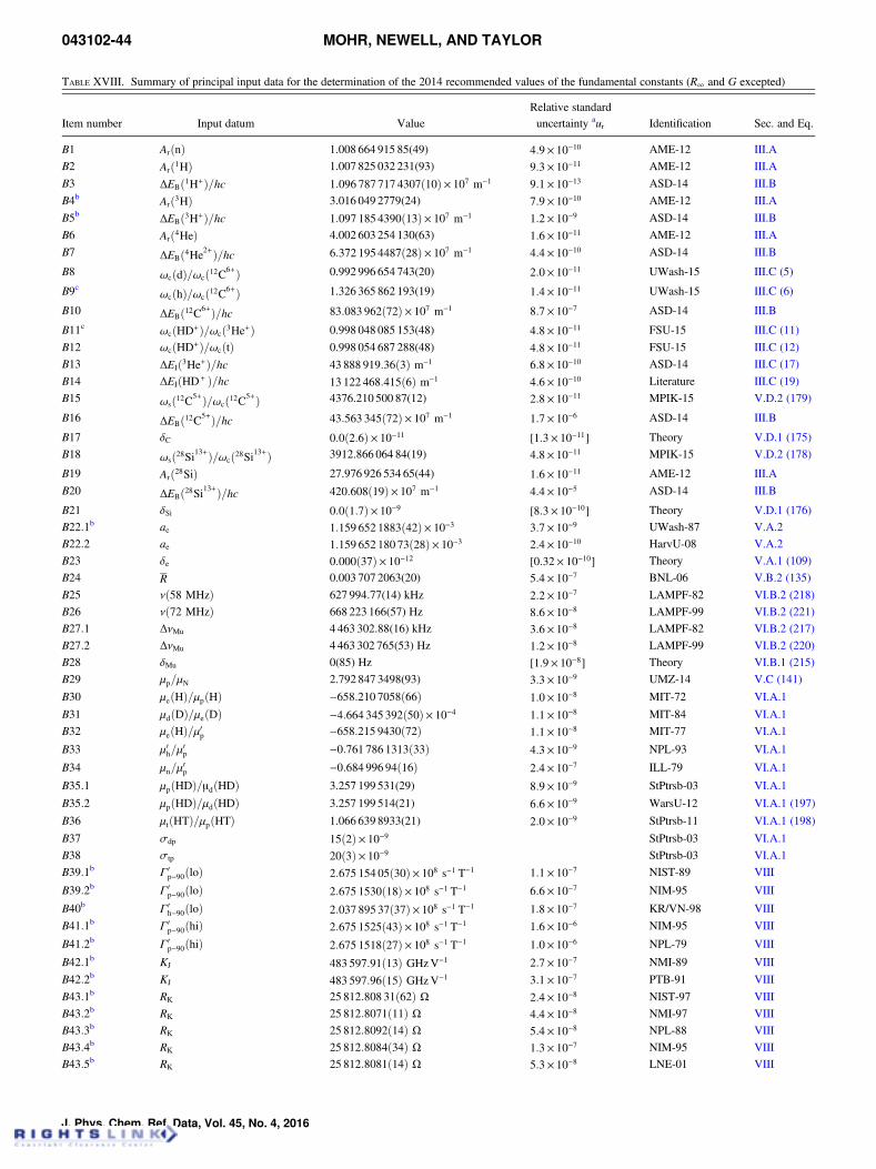
TABLE XVIII. Summary of principal input data for the determination of the 2014 recommended values of the fundamental constants (R∞ and G excepted)
Item number Input datum ValueRelative standarduncertainty aur Identification Sec. and Eq.
B1 ArðnÞ 1.008 664 915 85(49) 4:9× 10⁻¹⁰ AME-12 III.A
B2 Arð1HÞ 1.007 825 032 231(93) 9:3× 10⁻¹¹ AME-12 III.A
B3 ΔEBð1H+Þ=hc 1:096 787 717 4307ð10Þ× 107 m−1 9:1× 10⁻¹³ ASD-14 III.B
B4b Arð3HÞ 3.016 049 2779(24) 7:9× 10⁻¹⁰ AME-12 III.A
B5b ΔEBð3H+Þ=hc 1:097 185 4390ð13Þ× 107 m−1 1:2× 10⁻⁹ ASD-14 III.B
B6 Arð4HeÞ 4.002 603 254 130(63) 1:6× 10⁻¹¹ AME-12 III.A
B7 ΔEBð4He2+Þ=hc 6:372 195 4487ð28Þ× 107 m−1 4:4× 10⁻¹⁰ ASD-14 III.B
B8 ωcðdÞ=ωcð12C6+Þ 0.992 996 654 743(20) 2:0× 10−11 UWash-15 III.C (5)
B9c ωcðhÞ=ωcð12C6+Þ 1.326 365 862 193(19) 1:4× 10⁻¹¹ UWash-15 III.C (6)
B10 ΔEBð12C6+Þ=hc 83:083 962ð72Þ× 107 m−1 8:7× 10⁻⁷ ASD-14 III.B
B11c ωcðHD+Þ=ωcð3He+Þ 0.998 048 085 153(48) 4:8× 10⁻¹¹ FSU-15 III.C (11)
B12 ωcðHD+Þ=ωcðtÞ 0.998 054 687 288(48) 4:8× 10⁻¹¹ FSU-15 III.C (12)
B13 ΔEIð3He+Þ=hc 43 888 919:36ð3Þ m−1 6:8× 10⁻¹⁰ ASD-14 III.C (17)
B14 ΔEIðHD+ Þ=hc 13 122 468:415ð6Þ m−1 4:6× 10⁻¹⁰ Literature III.C (19)
B15 ωsð12C5+Þ=ωcð12C5+Þ 4376.210 500 87(12) 2:8× 10⁻¹¹ MPIK-15 V.D.2 (179)
B16 ΔEBð12C5+Þ=hc 43:563 345ð72Þ× 107 m−1 1:7× 10⁻⁶ ASD-14 III.B
B17 δC 0:0ð2:6Þ× 10−11 [1:3× 10⁻¹¹] Theory V.D.1 (175)
B18 ωsð28Si13+Þ=ωcð28Si13+Þ 3912.866 064 84(19) 4:8× 10⁻¹¹ MPIK-15 V.D.2 (178)
B19 Arð28SiÞ 27.976 926 534 65(44) 1:6× 10⁻¹¹ AME-12 III.A
B20 ΔEBð28Si13+Þ=hc 420:608ð19Þ× 107 m−1 4:4× 10⁻⁵ ASD-14 III.B
B21 δSi 0:0ð1:7Þ× 10−9 [8:3× 10⁻¹⁰] Theory V.D.1 (176)
B22:1b ae 1:159 652 1883ð42Þ× 10−3 3:7× 10⁻⁹ UWash-87 V.A.2
B22:2 ae 1:159 652 180 73ð28Þ× 10−3 2:4× 10⁻¹⁰ HarvU-08 V.A.2
B23 δe 0:000ð37Þ× 10−12 [0:32× 10−10] Theory V.A.1 (109)
B24 R 0.003 707 2063(20) 5:4× 10⁻⁷ BNL-06 V.B.2 (135)
B25 νð58 MHzÞ 627 994.77(14) kHz 2:2× 10⁻⁷ LAMPF-82 VI.B.2 (218)
B26 νð72 MHzÞ 668 223 166(57) Hz 8:6× 10⁻⁸ LAMPF-99 VI.B.2 (221)
B27:1 ΔνMu 4 463 302.88(16) kHz 3:6× 10⁻⁸ LAMPF-82 VI.B.2 (217)
B27:2 ΔνMu 4 463 302 765(53) Hz 1:2× 10⁻⁸ LAMPF-99 VI.B.2 (220)
B28 δMu 0(85) Hz [1:9× 10⁻⁸] Theory VI.B.1 (215)
B29 μp=μN 2.792 847 3498(93) 3:3× 10⁻⁹ UMZ-14 V.C (141)
B30 μeðHÞ=μpðHÞ −658:210 7058ð66Þ 1:0× 10−8 MIT-72 VI.A.1
B31 μdðDÞ=μeðDÞ −4:664 345 392ð50Þ× 10−4 1:1× 10⁻⁸ MIT-84 VI.A.1
B32 μeðHÞ=μ0p −658:215 9430ð72Þ 1:1× 10⁻⁸ MIT-77 VI.A.1
B33 μ0h=μ0p −0:761 786 1313ð33Þ 4:3× 10⁻⁹ NPL-93 VI.A.1
B34 μn=μ0p −0:684 996 94ð16Þ 2:4× 10⁻⁷ ILL-79 VI.A.1
B35:1 μpðHDÞ=μdðHDÞ 3.257 199 531(29) 8:9× 10⁻⁹ StPtrsb-03 VI.A.1
B35:2 μpðHDÞ=μdðHDÞ 3.257 199 514(21) 6:6× 10⁻⁹ WarsU-12 VI.A.1 (197)
B36 μtðHTÞ=μpðHTÞ 1.066 639 8933(21) 2:0× 10−9 StPtrsb-11 VI.A.1 (198)
B37 σdp 15ð2Þ× 10−9 StPtrsb-03 VI.A.1
B38 σtp 20ð3Þ× 10−9 StPtrsb-03 VI.A.1
B39:1b Γ0p−90ðloÞ 2:675 154 05ð30Þ× 108 s−1 T−1 1:1× 10⁻⁷ NIST-89 VIII
B39:2b Γ0p−90ðloÞ 2:675 1530ð18Þ× 108 s−1 T−1 6:6× 10⁻⁷ NIM-95 VIII
B40b Γ0h−90ðloÞ 2:037 895 37ð37Þ× 108 s−1 T−1 1:8× 10⁻⁷ KR/VN-98 VIII
B41:1b Γ0p−90ðhiÞ 2:675 1525ð43Þ× 108 s−1 T−1 1:6× 10⁻⁶ NIM-95 VIII
B41:2b Γ0p−90ðhiÞ 2:675 1518ð27Þ× 108 s−1 T−1 1:0× 10−6 NPL-79 VIII
B42:1b KJ 483 597:91ð13Þ GHzV−1 2:7× 10⁻⁷ NMI-89 VIII
B42:2b KJ 483 597:96ð15Þ GHzV−1 3:1× 10⁻⁷ PTB-91 VIII
B43:1b RK 25 812:808 31ð62Þ Ω 2:4× 10⁻⁸ NIST-97 VIII
B43:2b RK 25 812:8071ð11Þ Ω 4:4× 10⁻⁸ NMI-97 VIII
B43:3b RK 25 812:8092ð14Þ Ω 5:4× 10⁻⁸ NPL-88 VIII
B43:4b RK 25 812:8084ð34Þ Ω 1:3× 10⁻⁷ NIM-95 VIII
B43:5b RK 25 812:8081ð14Þ Ω 5:3× 10⁻⁸ LNE-01 VIII
043102-44 MOHR, NEWELL, AND TAYLOR
J. Phys. Chem. Ref. Data, Vol. 45, No. 4, 2016
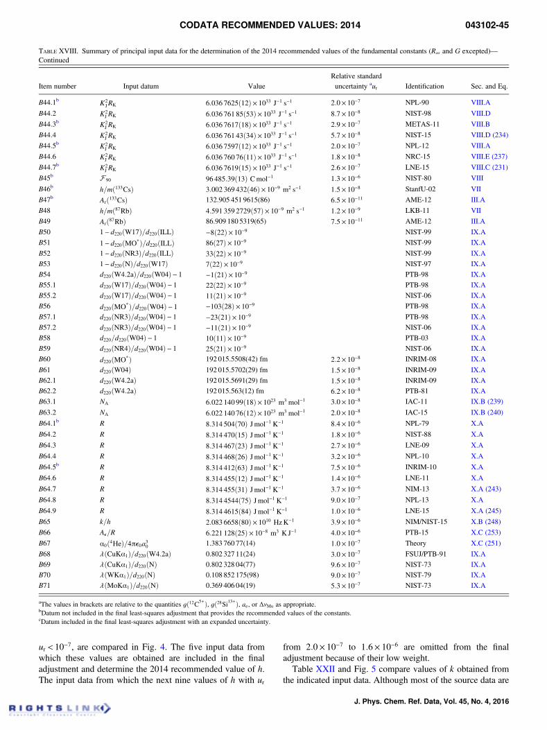
ur < 10−7, are compared in Fig. 4. The five input data fromwhich these values are obtained are included in the finaladjustment and determine the 2014 recommended value of h.The input data from which the next nine values of h with ur
from 2:0× 10−7 to 1:6× 10⁻⁶ are omitted from the finaladjustment because of their low weight.
Table XXII and Fig. 5 compare values of k obtained fromthe indicated input data. Although most of the source data are
TABLE XVIII. Summary of principal input data for the determination of the 2014 recommended values of the fundamental constants (R∞ and G excepted)—Continued
Item number Input datum ValueRelative standarduncertainty aur Identification Sec. and Eq.
B44:1b K2JRK 6:036 7625ð12Þ× 1033 J−1 s−1 2:0× 10−7 NPL-90 VIII.A
B44:2 K2J RK 6:036 761 85ð53Þ× 1033 J−1 s−1 8:7× 10⁻⁸ NIST-98 VIII.D
B44:3b K2J RK 6:036 7617ð18Þ× 1033 J−1 s−1 2:9× 10⁻⁷ METAS-11 VIII.B
B44:4 K2J RK 6:036 761 43ð34Þ× 1033 J−1 s−1 5:7× 10⁻⁸ NIST-15 VIII.D (234)
B44:5b K2J RK 6:036 7597ð12Þ× 1033 J−1 s−1 2:0× 10−7 NPL-12 VIII.A
B44:6 K2J RK 6:036 760 76ð11Þ× 1033 J−1 s−1 1:8× 10⁻⁸ NRC-15 VIII.E (237)
B44:7b K2J RK 6:036 7619ð15Þ× 1033 J−1 s−1 2:6× 10⁻⁷ LNE-15 VIII.C (231)
B45b F 90 96 485:39ð13Þ Cmol−1 1:3× 10⁻⁶ NIST-80 VIII
B46b h=mð133CsÞ 3:002 369 432ð46Þ× 10−9 m2 s−1 1:5× 10⁻⁸ StanfU-02 VII
B47b Arð133CsÞ 132.905 451 9615(86) 6:5× 10⁻¹¹ AME-12 III.A
B48 h=mð87RbÞ 4:591 359 2729ð57Þ× 10−9 m2 s−1 1:2× 10⁻⁹ LKB-11 VII
B49 Arð87RbÞ 86.909 180 5319(65) 7:5× 10⁻¹¹ AME-12 III.A
B50 1− d220ðW17Þ=d220ðILLÞ −8ð22Þ× 10−9 NIST-99 IX.A
B51 1− d220ðMO*Þ=d220ðILLÞ 86ð27Þ× 10−9 NIST-99 IX.A
B52 1− d220ðNR3Þ=d220ðILLÞ 33ð22Þ× 10−9 NIST-99 IX.A
B53 1− d220ðNÞ=d220ðW17Þ 7ð22Þ× 10−9 NIST-97 IX.A
B54 d220ðW4:2aÞ=d220ðW04Þ− 1 −1ð21Þ× 10−9 PTB-98 IX.A
B55:1 d220ðW17Þ=d220ðW04Þ− 1 22ð22Þ× 10−9 PTB-98 IX.A
B55:2 d220ðW17Þ=d220ðW04Þ− 1 11ð21Þ× 10−9 NIST-06 IX.A
B56 d220ðMO*Þ=d220ðW04Þ− 1 −103ð28Þ× 10−9 PTB-98 IX.A
B57:1 d220ðNR3Þ=d220ðW04Þ− 1 −23ð21Þ× 10−9 PTB-98 IX.A
B57:2 d220ðNR3Þ=d220ðW04Þ− 1 −11ð21Þ× 10−9 NIST-06 IX.A
B58 d220=d220ðW04Þ− 1 10ð11Þ× 10−9 PTB-03 IX.A
B59 d220ðNR4Þ=d220ðW04Þ− 1 25ð21Þ× 10−9 NIST-06 IX.A
B60 d220ðMO*Þ 192 015.5508(42) fm 2:2× 10⁻⁸ INRIM-08 IX.A
B61 d220ðW04Þ 192 015.5702(29) fm 1:5× 10⁻⁸ INRIM-09 IX.A
B62:1 d220ðW4:2aÞ 192 015.5691(29) fm 1:5× 10⁻⁸ INRIM-09 IX.A
B62:2 d220ðW4:2aÞ 192 015.563(12) fm 6:2× 10⁻⁸ PTB-81 IX.A
B63:1 NA 6:022 140 99ð18Þ× 1023 m3 mol−1 3:0× 10−8 IAC-11 IX.B (239)
B63:2 NA 6:022 140 76ð12Þ× 1023 m3 mol−1 2:0× 10−8 IAC-15 IX.B (240)
B64:1b R 8:314 504ð70Þ Jmol−1 K−1 8:4× 10⁻⁶ NPL-79 X.A
B64:2 R 8:314 470ð15Þ Jmol−1 K−1 1:8× 10⁻⁶ NIST-88 X.A
B64:3 R 8:314 467ð23Þ Jmol−1 K−1 2:7× 10⁻⁶ LNE-09 X.A
B64:4 R 8:314 468ð26Þ Jmol−1 K−1 3:2× 10⁻⁶ NPL-10 X.A
B64:5b R 8:314 412ð63Þ Jmol−1 K−1 7:5× 10⁻⁶ INRIM-10 X.A
B64:6 R 8:314 455ð12Þ Jmol−1 K−1 1:4× 10⁻⁶ LNE-11 X.A
B64:7 R 8:314 455ð31Þ Jmol−1 K−1 3:7× 10⁻⁶ NIM-13 X.A (243)
B64:8 R 8:314 4544ð75Þ Jmol−1 K−1 9:0× 10−7 NPL-13 X.A
B64:9 R 8:314 4615ð84Þ Jmol−1 K−1 1:0× 10−6 LNE-15 X.A (245)
B65 k=h 2:083 6658ð80Þ× 1010 HzK−1 3:9× 10⁻⁶ NIM/NIST-15 X.B (248)
B66 Ae=R 6:221 128ð25Þ× 10−8 m3 K J−1 4:0× 10−6 PTB-15 X.C (253)
B67 α0ð4HeÞ=4πe0a30 1.383 760 77(14) 1:0× 10−7 Theory X.C (251)
B68 λðCuKα1Þ=d220ðW4:2aÞ 0.802 327 11(24) 3:0× 10−7 FSUJ/PTB-91 IX.A
B69 λðCuKα1Þ=d220ðNÞ 0.802 328 04(77) 9:6× 10⁻⁷ NIST-73 IX.A
B70 λðWKα1Þ=d220ðNÞ 0.108 852 175(98) 9:0× 10−7 NIST-79 IX.A
B71 λðMoKα1Þ=d220ðNÞ 0.369 406 04(19) 5:3× 10⁻⁷ NIST-73 IX.A
aThe values in brackets are relative to the quantities gð12C5+Þ, gð28Si13+Þ, ae, or ΔνMu as appropriate.bDatum not included in the final least-squares adjustment that provides the recommended values of the constants.cDatum included in the final least-squares adjustment with an expanded uncertainty.
CODATA RECOMMENDED VALUES: 2014 043102-45
J. Phys. Chem. Ref. Data, Vol. 45, No. 4, 2016
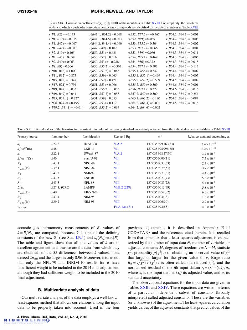
acoustic gas thermometry measurements of R, values ofk =R=NA are compared, because k is one of the definingconstants of the new SI (see Sec. I.B.1) and urðNAÞ≪urðRÞ.The table and figure show that all the values of k are inexcellent agreement, and thus so are the data from which theyare obtained; of the 55 differences between k values, noneexceed 2udiff and the largest is only 0.96. Moreover, it turns outthat only the NPL-79 and INRIM-10 results for R haveinsufficient weight to be included in the 2014 final adjustment,although they had sufficient weight to be included in the 2010final adjustment.
B. Multivariate analysis of data
Our multivariate analysis of the data employs a well-knownleast-squares method that allows correlations among the inputdata to be properly taken into account. Used in the four
previous adjustments, it is described in Appendix E ofCODATA-98 and the references cited therein. It is recalledfrom that appendix that a least-squares adjustment is charac-terized by the number of input data N, number of variables oradjusted constants M, degrees of freedom ν=N −M, statisticχ2, probability pðχ2jνÞ of obtaining an observed value of χ2
that large or larger for the given value of ν, Birge ratioRB =
ffiffiffiffiffiffiffiffiffiffiχ2=ν
p(χ2=ν is often called the reduced χ2), and the
normalized residual of the ith input datum ri = ðxi − ÆxiæÞ=ui,where xi is the input datum, Æxiæ its adjusted value, and ui itsstandard uncertainty.
The observational equations for the input data are given inTables XXIII and XXIV. These equations are written in termsof a particular independent subset of constants (broadlyinterpreted) called adjusted constants. These are the variables(or unknowns) of the adjustment. The least-squares calculationyields values of the adjusted constants that predict values of the
TABLE XIX. Correlation coefficients rðxi, xjÞ≥ 0:001 of the input data in Table XVIII. For simplicity, the two itemsof data to which a particular correlation coefficient corresponds are identified by their item numbers in Table XVIII
rðB1, B2Þ=−0:133 rðB42:1, B64:2Þ= 0:068 rðB52, B57:2Þ=−0:367 rðB64:2, B64:7Þ= 0:001rðB1, B19Þ=−0:015 rðB44:1, B44:5Þ= 0:003 rðB52, B59Þ= 0:065 rðB64:2, B64:8Þ= 0:003rðB1, B47Þ=−0:007 rðB44:2, B44:4Þ= 0:090 rðB53, B55:2Þ= 0:504 rðB64:3, B64:4Þ= 0:002rðB1, B49Þ=−0:007 rðB47, B49Þ= 0:102 rðB53, B57:2Þ= 0:066 rðB64:3, B64:5Þ= 0:001rðB2, B19Þ= 0:165 rðB50, B51Þ= 0:421 rðB53, B59Þ= 0:066 rðB64:3, B64:6Þ= 0:011rðB2, B47Þ= 0:058 rðB50, B52Þ= 0:516 rðB54, B55:1Þ= 0:469 rðB64:3, B64:8Þ= 0:006rðB2, B49Þ= 0:063 rðB50, B53Þ=−0:288 rðB54, B56Þ= 0:372 rðB64:3, B64:9Þ= 0:018rðB8, B9Þ= 0:306 rðB50, B55:2Þ=−0:367 rðB54, B57:1Þ= 0:502 rðB64:4, B64:6Þ= 0:113rðB10, B16Þ= 1:000 rðB50, B57:2Þ= 0:065 rðB55:1, B56Þ= 0:347 rðB64:4, B64:8Þ= 0:007rðB11, B12Þ= 0:875 rðB50, B59Þ= 0:065 rðB55:1, B57:1Þ= 0:469 rðB64:4, B64:9Þ= 0:005rðB15, B18Þ= 0:347 rðB51, B52Þ= 0:421 rðB55:2, B57:2Þ= 0:509 rðB64:5, B64:9Þ= 0:002rðB17, B21Þ= 0:791 rðB51, B53Þ= 0:096 rðB55:2, B59Þ= 0:509 rðB64:6, B64:7Þ= 0:001rðB19, B47Þ= 0:033 rðB51, B55:2Þ= 0:053 rðB56, B57:1Þ= 0:372 rðB64:6, B64:8Þ= 0:016rðB19, B49Þ= 0:041 rðB51, B57:2Þ= 0:053 rðB57:2, B59Þ= 0:509 rðB64:6, B64:9Þ= 0:254rðB25, B27:1Þ= 0:227 rðB51, B59Þ= 0:053 rðB63:1, B63:2Þ= 0:170 rðB64:7, B64:8Þ= 0:084rðB26, B27:2Þ= 0:195 rðB52, B53Þ= 0:117 rðB64:2, B64:4Þ= 0:001 rðB64:8, B64:9Þ= 0:016rðB39:2, B41:1Þ=−0:014 rðB52, B55:2Þ= 0:065 rðB64:2, B64:6Þ= 0:002
TABLE XX. Inferred values of the fine-structure constant α in order of increasing standard uncertainty obtained from the indicated experimental data in Table XVIII
Primary source Item number Identification Sec. and Eq. α−1 Relative standard uncertainty ur
ae B22:2 HarvU-08 V.A.2 137.035 999 160(33) 2:4× 10⁻¹⁰
h=mð87RbÞ B48 LKB-11 VII 137.035 998 996(85) 6:2× 10⁻¹⁰
ae B22:1 UWash-87 V.A.2 137.035 998 27(50) 3:7× 10⁻⁹
h=mð133CsÞ B46 StanfU-02 VII 137.036 0000(11) 7:7× 10⁻⁹
RK B43:1 NIST-97 VIII 137.036 0037(33) 2:4× 10⁻⁸
Γ0p−90ðloÞ B39:1 NIST-89 VIII 137.035 9879(51) 3:7× 10⁻⁸
RK B43:2 NMI-97 VIII 137.035 9973(61) 4:4× 10⁻⁸
RK B43:5 LNE-01 VIII 137.036 0023(73) 5:3× 10⁻⁸
RK B43:3 NPL-88 VIII 137.036 0083(73) 5:4× 10⁻⁸
ΔνMu B27:1, B27:2 LAMPF VI.B.2 (228) 137.036 0013(79) 5:8× 10⁻⁸
Γ0h−90ðloÞ B40 KR/VN-98 VIII 137.035 9852(82) 6:0× 10−8
RK B43:4 NIM-95 VIII 137.036 004(18) 1:3× 10⁻⁷
Γ0p−90ðloÞ B39:2 NIM-95 VIII 137.036 006(30) 2:2× 10⁻⁷
νH, νD IV.A.1.m (71) 137.035 992(55) 4:0× 10−7
043102-46 MOHR, NEWELL, AND TAYLOR
J. Phys. Chem. Ref. Data, Vol. 45, No. 4, 2016
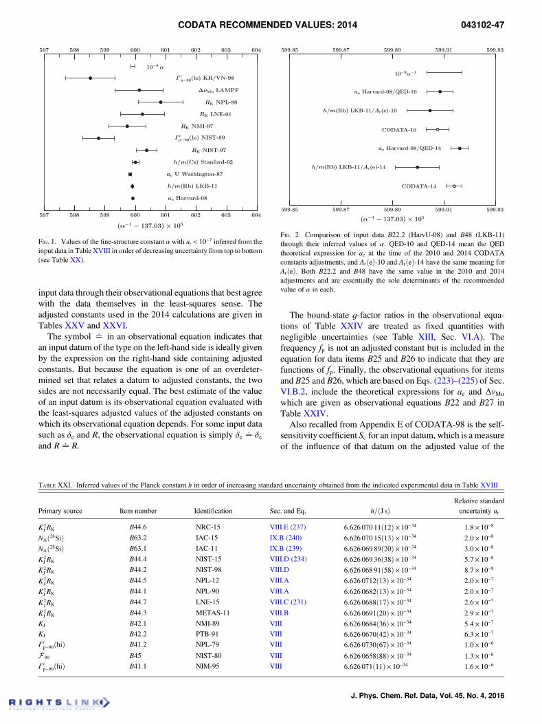
input data through their observational equations that best agreewith the data themselves in the least-squares sense. Theadjusted constants used in the 2014 calculations are given inTables XXV and XXVI.
The symbol ^ in an observational equation indicates thatan input datum of the type on the left-hand side is ideally givenby the expression on the right-hand side containing adjustedconstants. But because the equation is one of an overdeter-mined set that relates a datum to adjusted constants, the twosides are not necessarily equal. The best estimate of the valueof an input datum is its observational equation evaluated withthe least-squares adjusted values of the adjusted constants onwhich its observational equation depends. For some input datasuch as δe and R, the observational equation is simply δe ^ δeand R^R.
The bound-state g-factor ratios in the observational equa-tions of Table XXIV are treated as fixed quantities withnegligible uncertainties (see Table XIII, Sec. VI.A). Thefrequency fp is not an adjusted constant but is included in theequation for data items B25 and B26 to indicate that they arefunctions of fp. Finally, the observational equations for itemsand B25 and B26, which are based on Eqs. (223)–(225) of Sec.VI.B.2, include the theoretical expressions for ae and ΔνMu
which are given as observational equations B22 and B27 inTable XXIV.
Also recalled from Appendix E of CODATA-98 is the self-sensitivity coefficient Sc for an input datum, which is a measureof the influence of that datum on the adjusted value of the
FIG. 1. Values of the fine-structure constant α with ur < 10−7 inferred from theinput data in Table XVIII in order of decreasing uncertainty from top to bottom(see Table XX).
FIG. 2. Comparison of input data B22:2 (HarvU-08) and B48 (LKB-11)through their inferred values of α. QED-10 and QED-14 mean the QEDtheoretical expression for ae at the time of the 2010 and 2014 CODATAconstants adjustments, and ArðeÞ-10 and ArðeÞ-14 have the same meaning forArðeÞ. Both B22:2 and B48 have the same value in the 2010 and 2014adjustments and are essentially the sole determinants of the recommendedvalue of α in each.
TABLE XXI. Inferred values of the Planck constant h in order of increasing standard uncertainty obtained from the indicated experimental data in Table XVIII
Primary source Item number Identification Sec. and Eq. h=ðJ sÞRelative standarduncertainty ur
K2J RK B44:6 NRC-15 VIII.E (237) 6:626 070 11ð12Þ× 10−34 1:8× 10⁻⁸
NAð28SiÞ B63:2 IAC-15 IX.B (240) 6:626 070 15ð13Þ× 10−34 2:0× 10−8
NAð28SiÞ B63:1 IAC-11 IX.B (239) 6:626 069 89ð20Þ× 10−34 3:0× 10−8
K2J RK B44:4 NIST-15 VIII.D (234) 6:626 069 36ð38Þ× 10−34 5:7× 10⁻⁸
K2J RK B44:2 NIST-98 VIII.D 6:626 068 91ð58Þ× 10−34 8:7× 10⁻⁸
K2JRK B44:5 NPL-12 VIII.A 6:626 0712ð13Þ× 10−34 2:0× 10−7
K2J RK B44:1 NPL-90 VIII.A 6:626 0682ð13Þ× 10−34 2:0× 10−7
K2JRK B44:7 LNE-15 VIII.C (231) 6:626 0688ð17Þ× 10−34 2:6× 10⁻⁷
K2J RK B44:3 METAS-11 VIII.B 6:626 0691ð20Þ× 10−34 2:9× 10⁻⁷
KJ B42:1 NMI-89 VIII 6:626 0684ð36Þ× 10−34 5:4× 10⁻⁷
KJ B42:2 PTB-91 VIII 6:626 0670ð42Þ× 10−34 6:3× 10⁻⁷
Γ0p−90ðhiÞ B41:2 NPL-79 VIII 6:626 0730ð67Þ× 10−34 1:0× 10−6
F 90 B45 NIST-80 VIII 6:626 0658ð88Þ× 10−34 1:3× 10⁻⁶
Γ0p−90ðhiÞ B41:1 NIM-95 VIII 6:626 071ð11Þ× 10−34 1:6× 10⁻⁶
CODATA RECOMMENDED VALUES: 2014 043102-47
J. Phys. Chem. Ref. Data, Vol. 45, No. 4, 2016
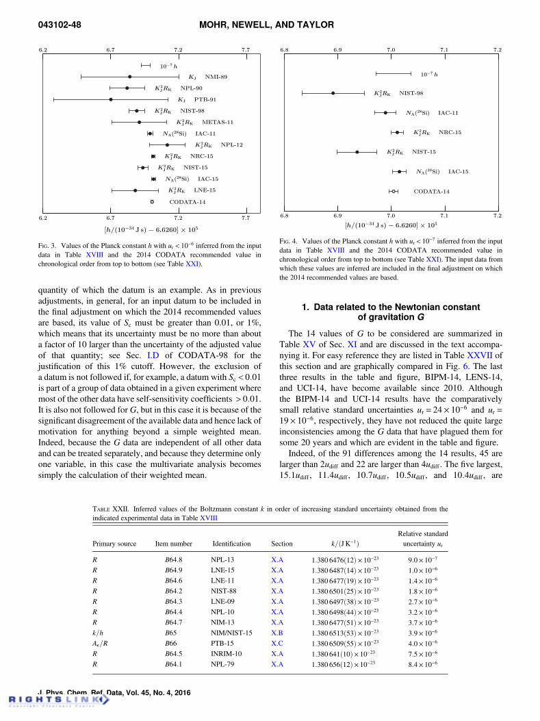
quantity of which the datum is an example. As in previousadjustments, in general, for an input datum to be included inthe final adjustment on which the 2014 recommended valuesare based, its value of Sc must be greater than 0.01, or 1%,which means that its uncertainty must be no more than abouta factor of 10 larger than the uncertainty of the adjusted valueof that quantity; see Sec. I.D of CODATA-98 for thejustification of this 1% cutoff. However, the exclusion ofa datum is not followed if, for example, a datum with Sc < 0:01is part of a group of data obtained in a given experiment wheremost of the other data have self-sensitivity coefficients > 0:01.It is also not followed for G, but in this case it is because of thesignificant disagreement of the available data and hence lack ofmotivation for anything beyond a simple weighted mean.Indeed, because the G data are independent of all other dataand can be treated separately, and because they determine onlyone variable, in this case the multivariate analysis becomessimply the calculation of their weighted mean.
1. Data related to the Newtonian constantof gravitation G
The 14 values of G to be considered are summarized inTable XV of Sec. XI and are discussed in the text accompa-nying it. For easy reference they are listed in Table XXVII ofthis section and are graphically compared in Fig. 6. The lastthree results in the table and figure, BIPM-14, LENS-14,and UCI-14, have become available since 2010. Althoughthe BIPM-14 and UCI-14 results have the comparativelysmall relative standard uncertainties ur = 24× 10−6 and ur =19× 10−6, respectively, they have not reduced the quite largeinconsistencies among the G data that have plagued them forsome 20 years and which are evident in the table and figure.
Indeed, of the 91 differences among the 14 results, 45 arelarger than 2udiff and 22 are larger than 4udiff . The five largest,15:1udiff , 11:4udiff , 10:7udiff , 10:5udiff , and 10:4udiff , are
TABLE XXII. Inferred values of the Boltzmann constant k in order of increasing standard uncertainty obtained from theindicated experimental data in Table XVIII
Primary source Item number Identification Section k=ðJ K−1ÞRelative standarduncertainty ur
R B64:8 NPL-13 X.A 1:380 6476ð12Þ× 10−23 9:0× 10−7
R B64:9 LNE-15 X.A 1:380 6487ð14Þ× 10−23 1:0× 10−6
R B64:6 LNE-11 X.A 1:380 6477ð19Þ× 10−23 1:4× 10⁻⁶
R B64:2 NIST-88 X.A 1:380 6501ð25Þ× 10−23 1:8× 10⁻⁶
R B64:3 LNE-09 X.A 1:380 6497ð38Þ× 10−23 2:7× 10⁻⁶
R B64:4 NPL-10 X.A 1:380 6498ð44Þ× 10−23 3:2× 10⁻⁶
R B64:7 NIM-13 X.A 1:380 6477ð51Þ× 10−23 3:7× 10⁻⁶
k=h B65 NIM/NIST-15 X.B 1:380 6513ð53Þ× 10−23 3:9× 10⁻⁶
Ae=R B66 PTB-15 X.C 1:380 6509ð55Þ× 10−23 4:0× 10−6
R B64:5 INRIM-10 X.A 1:380 641ð10Þ× 10−23 7:5× 10⁻⁶
R B64:1 NPL-79 X.A 1:380 656ð12Þ× 10−23 8:4× 10⁻⁶
FIG. 4. Values of the Planck constant h with ur < 10−7 inferred from the inputdata in Table XVIII and the 2014 CODATA recommended value inchronological order from top to bottom (see Table XXI). The input data fromwhich these values are inferred are included in the final adjustment on whichthe 2014 recommended values are based.
FIG. 3. Values of the Planck constant h with ur < 10−6 inferred from the inputdata in Table XVIII and the 2014 CODATA recommended value inchronological order from top to bottom (see Table XXI).
043102-48 MOHR, NEWELL, AND TAYLOR
J. Phys. Chem. Ref. Data, Vol. 45, No. 4, 2016
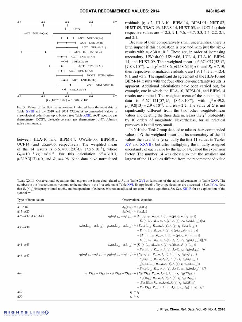
between JILA-10 and BIPM-14, UWash-00, BIPM-01,UCI-14, and UZur-06, respectively. The weighted meanof the 14 results is 6:674 083ð50ÞG0 [7:5× 10⁻⁶], whereG0 = 10−11 kg−1 m3 s−2. For this calculation χ2 = 319:3,pð319:3j13Þ≈ 0, and RB = 4:96. Nine data have normalized
residuals jrij> 2: JILA-10, BIPM-14, BIPM-01, NIST-82,HUST-09, TR&D-96, LENS-14, HUST-05, and UCI-14; theirrespective values are −12:5, 9.1, 5.6, −3:7, 3.3, 2.4, 2.2, 2.1,and 2.1.
Because of their comparatively small uncertainties, there islittle impact if this calculation is repeated with just the six Gresults with ur < 30× 10−6. These are, in order of increasinguncertainty, UWash-00, UZur-06, UCI-14, JILA-10, BIPM-14, and HUST-09. Their weighted mean is 6:674 077ð52ÞG0
[7:8× 10⁻⁶], with χ2 = 258:6, pð258:6j13Þ≈ 0, and RB = 7:19;their respective normalized residuals ri are 1.9, 1.4, 2.2, −12:4,9.1, and−3:3. The significant disagreement of the JILA-10 andBIPM-14 results with the four other low-uncertainty results isapparent. Additional calculations have been carried out, forexample, one in which the JILA-10, BIPM-01, and BIPM-14results are omitted. The weighted mean of the remaining 11data is 6:674 121ð57ÞG0 [8:6× 10⁻⁶], with χ2 = 49:8,pð49:8j13Þ= 2:9× 10⁻⁶, and RB = 2:2. The value of G is notsignificantly different from the two other weighted-meanvalues and deleting the three data increases the χ2 probabilityby 10 orders of magnitude. Nevertheless, for all practicalpurposes it is still very small.
In 2010 the Task Group decided to take as the recommendedvalue of G the weighted mean and its uncertainty of the 11values then available (essentially the first 11 values in TablesXV and XXVII), but after multiplying the initially assigneduncertainty of each value by the factor 14, called the expansionfactor. The number 14 was chosen so that the smallest andlargest of the 11 values differed from the recommended value
FIG. 5. Values of the Boltzmann constant k inferred from the input data inTable XVIII and the 2010 and 2014 CODATA recommended values inchronological order from top to bottom (see Table XXII). AGT: acoustic gasthermometry; DCGT: dielectric-constant gas thermometry; JNT: Johnsonnoise thermometry.
TABLE XXIII. Observational equations that express the input data related to R∞ in Table XVI as functions of the adjusted constants in Table XXV. Thenumbers in the first column correspond to the numbers in the first column of Table XVI. Energy levels of hydrogenic atoms are discussed in Sec. IV.A. Notethat EXðnLjÞ=h is proportional to cR∞ and independent of h, hence h is not an adjusted constant in these equations. See Sec. XIII.B for an explanation of thesymbol^
Type of input datum Observational equation
A1–A16 δHðnLjÞ^ δHðnLjÞA17–A25 δDðnLjÞ^ δDðnLjÞA26–A32, A39, A40 νHðn1L1 j1 − n2L2 j2 Þ^ ½EHðn2L2 j2 ;R∞,α,ArðeÞ,ArðpÞ, rp, δHðn2L2 j2 ÞÞ
−EHðn1L1 j1 ;R∞, α, ArðeÞ, ArðpÞ, rp, δHðn1L1 j1 ÞÞ�=hA33–A38 νHðn1L1 j1 − n2L2 j2 Þ− 1
4νHðn3L3 j3 − n4L4 j4 Þ^ fEHðn2L2 j2 ;R∞,α,ArðeÞ,ArðpÞ, rp, δHðn2L2 j2 ÞÞ−EHðn1L1 j1 ;R∞,α,ArðeÞ,ArðpÞ, rp, δHðn1L1 j1 ÞÞ− 1
4½EHðn4L4 j4 ;R∞,α,ArðeÞ,ArðpÞ, rp, δHðn4L4 j4 ÞÞ−EHðn3L3 j3 ;R∞, α, ArðeÞ, ArðpÞ, rp, δHðn3L3 j3 ÞÞ�g=h
A41–A45 νDðn1L1 j1 − n2L2 j2 Þ^ ½EDðn2L2 j2 ;R∞,α,ArðeÞ,ArðdÞ, rd, δDðn2L2 j2 ÞÞ−EDðn1L1 j1 ;R∞, α, ArðeÞ, ArðdÞ, rd, δDðn1L1 j1 ÞÞ�=h
A46–A47 νDðn1L1 j1 − n2L2 j2 Þ− 14νDðn3L3 j3 − n4L4 j4 Þ^ fEDðn2L2 j2 ;R∞,α,ArðeÞ,ArðdÞ, rd, δDðn2L2 j2 ÞÞ
−EDðn1L1 j1 ;R∞,α,ArðeÞ,ArðdÞ, rd, δDðn1L1 j1 ÞÞ− 1
4½EDðn4L4 j4 ;R∞,α,ArðeÞ,ArðdÞ, rd, δDðn4L4 j4 ÞÞ−EDðn3L3 j3 ;R∞, α, ArðeÞ, ArðdÞ, rd, δDðn3L3 j3 ÞÞ�g=h
A48 νDð1S1=2 − 2S1=2Þ− νHð1S1=2 − 2S1=2Þ^ fEDð2S1=2;R∞,α,ArðeÞ,ArðdÞ, rd, δDð2S1=2ÞÞ−EDð1S1=2;R∞,α,ArðeÞ,ArðdÞ, rd, δDð1S1=2ÞÞ− ½EHð2S1=2;R∞,α,ArðeÞ,ArðpÞ, rp, δHð2S1=2ÞÞ−EHð1S1=2;R∞, α, ArðeÞ, ArðpÞ, rp, δHð1S1=2ÞÞ�g=h
A49 rp ^ rpA50 rd ^ rd
CODATA RECOMMENDED VALUES: 2014 043102-49
J. Phys. Chem. Ref. Data, Vol. 45, No. 4, 2016
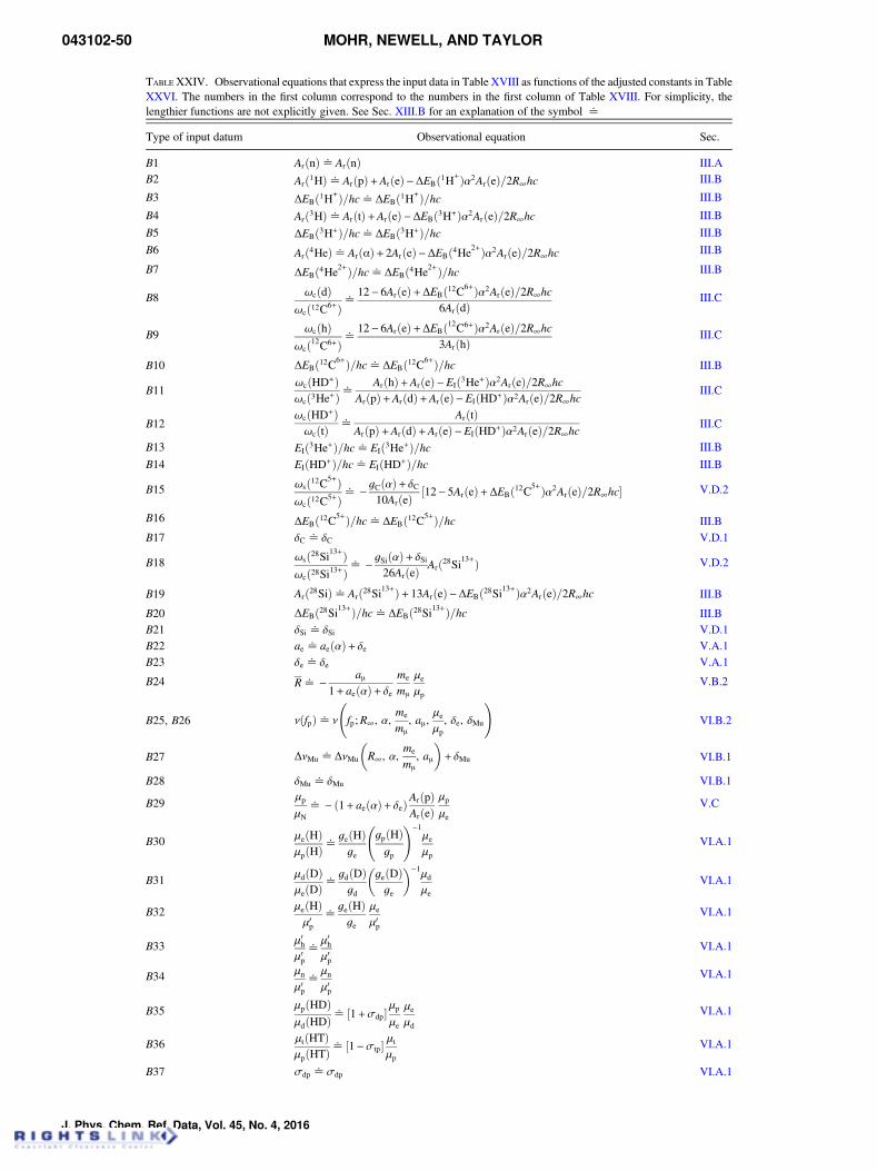
TABLE XXIV. Observational equations that express the input data in Table XVIII as functions of the adjusted constants in TableXXVI. The numbers in the first column correspond to the numbers in the first column of Table XVIII. For simplicity, thelengthier functions are not explicitly given. See Sec. XIII.B for an explanation of the symbol ^
Type of input datum Observational equation Sec.
B1 ArðnÞ^ArðnÞ III.AB2 Arð1HÞ^ArðpÞ+ArðeÞ−ΔEBð1H+Þα2ArðeÞ=2R∞hc III.B
B3 ΔEBð1H+Þ=hc^ΔEBð1H+Þ=hc III.B
B4 Arð3HÞ^ArðtÞ+ArðeÞ−ΔEBð3H+Þα2ArðeÞ=2R∞hc III.B
B5 ΔEBð3H+Þ=hc^ΔEBð3H+Þ=hc III.B
B6 Arð4HeÞ^ArðαÞ+ 2ArðeÞ−ΔEBð4He2+Þα2ArðeÞ=2R∞hc III.B
B7 ΔEBð4He2+Þ=hc^ΔEBð4He2+Þ=hc III.B
B8 ωcðdÞωcð12C6+Þ^
12− 6ArðeÞ+ΔEBð12C6+Þα2ArðeÞ=2R∞hc6ArðdÞ
III.C
B9ωcðhÞ
ωcð12C6+Þ^12− 6ArðeÞ+ΔEBð12C6+Þα2ArðeÞ=2R∞hc
3ArðhÞIII.C
B10 ΔEBð12C6+Þ=hc^ΔEBð12C6+Þ=hc III.B
B11ωcðHD+Þωcð3He+Þ^
ArðhÞ+ArðeÞ−EIð3He+Þα2ArðeÞ=2R∞hcArðpÞ+ArðdÞ+ArðeÞ−EIðHD+Þα2ArðeÞ=2R∞hc
III.C
B12ωcðHD+ÞωcðtÞ ^
ArðtÞArðpÞ+ArðdÞ+ArðeÞ−EIðHD+Þα2ArðeÞ=2R∞hc
III.C
B13 EIð3He+Þ=hc^EIð3He+Þ=hc III.B
B14 EIðHD+Þ=hc^EIðHD+Þ=hc III.B
B15 ωsð12C5+Þωcð12C5+Þ^ − gCðαÞ+ δC
10ArðeÞ ½12− 5ArðeÞ+ΔEBð12C5+Þα2ArðeÞ=2R∞hc� V.D.2
B16 ΔEBð12C5+Þ=hc^ΔEBð12C5+Þ=hc III.BB17 δC ^ δC V.D.1
B18 ωsð28Si13+Þωcð28Si13+Þ
^ − gSiðαÞ+ δSi
26ArðeÞ Arð28Si13+Þ V.D.2
B19 Arð28SiÞ^Arð28Si13+Þ+ 13ArðeÞ−ΔEBð28Si13+Þα2ArðeÞ=2R∞hc III.B
B20 ΔEBð28Si13+Þ=hc^ΔEBð28Si13+Þ=hc III.BB21 δSi ^ δSi V.D.1B22 ae ^ aeðαÞ+ δe V.A.1B23 δe ^ δe V.A.1
B24 R^ − aμ1+ aeðαÞ+ δe
me
mμ
μe
μpV.B.2
B25, B26 νðfpÞ^ ν
fp;R∞, α,
me
mμ
, aμ,μe
μp, δe, δMu
!VI.B.2
B27 ΔνMu ^ΔνMu
R∞, α,
me
mμ
, aμ
�+ δMu VI.B.1
B28 δMu ^ δMu VI.B.1
B29μp
μN^ − ð1+ aeðαÞ+ δeÞArðpÞ
ArðeÞμp
μeV.C
B30 μeðHÞμpðHÞ
^geðHÞge
gpðHÞgp
!−1μe
μpVI.A.1
B31μdðDÞμeðDÞ
^gdðDÞgd
geðDÞge
�−1μd
μeVI.A.1
B32 μeðHÞμ0p
^geðHÞge
μe
μ0pVI.A.1
B33 μ0hμ0p
^μ0hμ0p
VI.A.1
B34 μn
μ0p^
μn
μ0pVI.A.1
B35 μpðHDÞμdðHDÞ
^ ½1+σdp�μp
μe
μe
μd
VI.A.1
B36 μtðHTÞμpðHTÞ
^ ½1−σtp� μtμp
VI.A.1
B37 σdp ^σdp VI.A.1
043102-50 MOHR, NEWELL, AND TAYLOR
J. Phys. Chem. Ref. Data, Vol. 45, No. 4, 2016
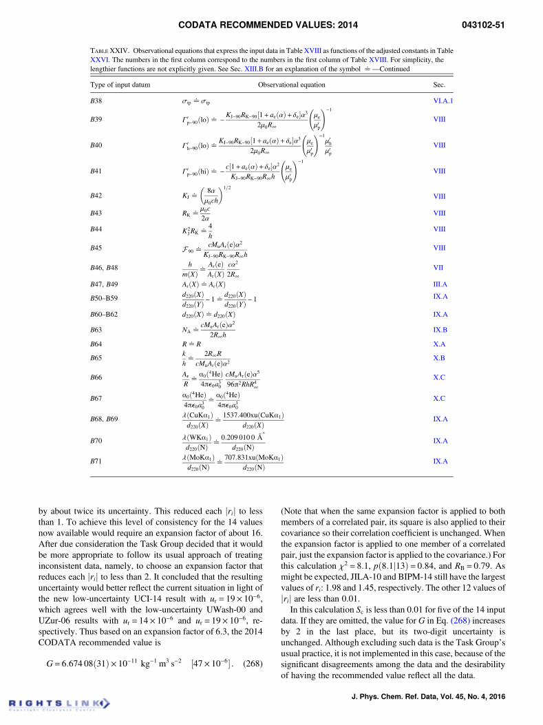
by about twice its uncertainty. This reduced each jrij to lessthan 1. To achieve this level of consistency for the 14 valuesnow available would require an expansion factor of about 16.After due consideration the Task Group decided that it wouldbe more appropriate to follow its usual approach of treatinginconsistent data, namely, to choose an expansion factor thatreduces each jrij to less than 2. It concluded that the resultinguncertainty would better reflect the current situation in light ofthe new low-uncertainty UCI-14 result with ur = 19× 10−6,which agrees well with the low-uncertainty UWash-00 andUZur-06 results with ur = 14× 10−6 and ur = 19× 10−6, re-spectively. Thus based on an expansion factor of 6.3, the 2014CODATA recommended value is
G= 6:674 08ð31Þ× 10−11 kg−1 m3 s−2 ½47× 10−6� . (268)
(Note that when the same expansion factor is applied to bothmembers of a correlated pair, its square is also applied to theircovariance so their correlation coefficient is unchanged. Whenthe expansion factor is applied to one member of a correlatedpair, just the expansion factor is applied to the covariance.) Forthis calculation χ2 = 8:1, pð8:1j13Þ= 0:84, and RB = 0:79. Asmight be expected, JILA-10 and BIPM-14 still have the largestvalues of ri: 1.98 and 1.45, respectively. The other 12 values ofjrij are less than 0.01.
In this calculation Sc is less than 0.01 for five of the 14 inputdata. If they are omitted, the value for G in Eq. (268) increasesby 2 in the last place, but its two-digit uncertainty isunchanged. Although excluding such data is the Task Group’susual practice, it is not implemented in this case, because of thesignificant disagreements among the data and the desirabilityof having the recommended value reflect all the data.
TABLE XXIV. Observational equations that express the input data in Table XVIII as functions of the adjusted constants in TableXXVI. The numbers in the first column correspond to the numbers in the first column of Table XVIII. For simplicity, thelengthier functions are not explicitly given. See Sec. XIII.B for an explanation of the symbol ^—Continued
Type of input datum Observational equation Sec.
B38 σtp ^σtp VI.A.1
B39 Γ0p−90ðloÞ^ −KJ−90RK−90½1+ aeðαÞ+ δe�α3
2μ0R∞
μe
μ0p
!−1VIII
B40 Γ0h−90ðloÞ^
KJ−90RK−90½1+ aeðαÞ+ δe�α3
2μ0R∞
μe
μ0p
!−1μ0hμ0p
VIII
B41 Γ0p−90ðhiÞ^ − c½1+ aeðαÞ+ δe�α2
KJ−90RK−90R∞h
μe
μ0p
!−1VIII
B42 KJ ^
8αμ0ch
�1=2
VIII
B43 RK ^μ0c2α
VIII
B44 K2JRK ^
4h
VIII
B45 F 90 ^cMuArðeÞα2
KJ−90RK−90R∞hVIII
B46, B48 hmðXÞ^
ArðeÞArðXÞ
cα2
2R∞VII
B47, B49 ArðXÞ^ArðXÞ III.A
B50–B59 d220ðXÞd220ðYÞ− 1^
d220ðXÞd220ðYÞ− 1 IX.A
B60–B62 d220ðXÞ^ d220ðXÞ IX.A
B63 NA ^cMuArðeÞα2
2R∞hIX.B
B64 R^R X.A
B65kh^
2R∞RcMuArðeÞα2
X.B
B66 Ae
R^
α0ð4HeÞ4πe0a30
cMuArðeÞα5
96π2RhR4∞
X.C
B67 α0ð4HeÞ4πe0a30
^α0ð4HeÞ4πe0a30
X.C
B68, B69 λðCuKα1Þd220ðXÞ ^
1537:400xuðCuKα1Þd220ðXÞ
IX.A
B70 λðWKα1Þd220ðNÞ ^
0:209 010 0 A*
d220ðNÞIX.A
B71 λðMoKα1Þd220ðNÞ ^
707:831xuðMoKα1Þd220ðNÞ
IX.A
CODATA RECOMMENDED VALUES: 2014 043102-51
J. Phys. Chem. Ref. Data, Vol. 45, No. 4, 2016
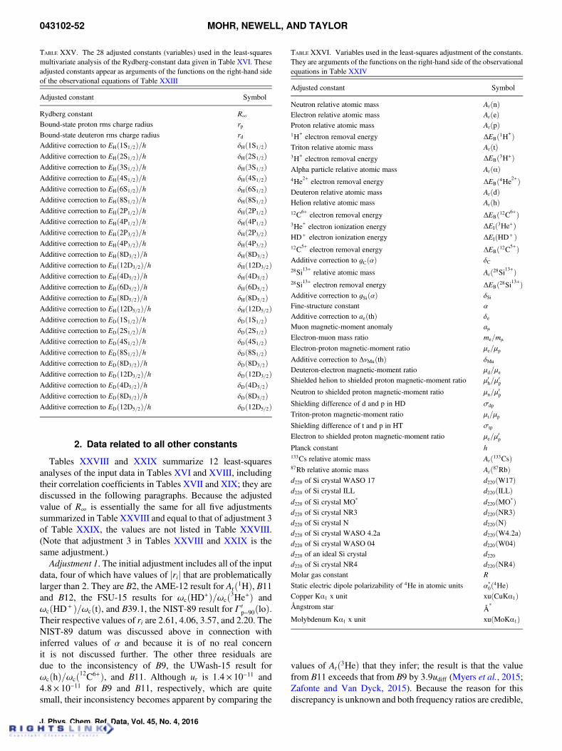
2. Data related to all other constants
Tables XXVIII and XXIX summarize 12 least-squaresanalyses of the input data in Tables XVI and XVIII, includingtheir correlation coefficients in Tables XVII and XIX; they arediscussed in the following paragraphs. Because the adjustedvalue of R∞ is essentially the same for all five adjustmentssummarized in Table XXVIII and equal to that of adjustment 3of Table XXIX, the values are not listed in Table XXVIII.(Note that adjustment 3 in Tables XXVIII and XXIX is thesame adjustment.)
Adjustment 1. The initial adjustment includes all of the inputdata, four of which have values of jrij that are problematicallylarger than 2. They are B2, the AME-12 result for Arð1HÞ, B11and B12, the FSU-15 results for ωcðHD+Þ=ωcð3He+Þ andωcðHD+ Þ=ωcðtÞ, and B39:1, the NIST-89 result for Γ0
p−90ðloÞ.Their respective values of ri are 2.61, 4.06, 3.57, and 2.20. TheNIST-89 datum was discussed above in connection withinferred values of α and because it is of no real concernit is not discussed further. The other three residuals aredue to the inconsistency of B9, the UWash-15 result forωcðhÞ=ωcð12C6+Þ, and B11. Although ur is 1:4× 10⁻¹¹ and4:8× 10⁻¹¹ for B9 and B11, respectively, which are quitesmall, their inconsistency becomes apparent by comparing the
values of Arð3HeÞ that they infer; the result is that the valuefrom B11 exceeds that from B9 by 3:9udiff (Myers et al., 2015;Zafonte and Van Dyck, 2015). Because the reason for thisdiscrepancy is unknown and both frequency ratios are credible,
TABLE XXV. The 28 adjusted constants (variables) used in the least-squaresmultivariate analysis of the Rydberg-constant data given in Table XVI. Theseadjusted constants appear as arguments of the functions on the right-hand sideof the observational equations of Table XXIII
Adjusted constant Symbol
Rydberg constant R∞Bound-state proton rms charge radius rpBound-state deuteron rms charge radius rdAdditive correction to EHð1S1=2Þ=h δHð1S1=2ÞAdditive correction to EHð2S1=2Þ=h δHð2S1=2ÞAdditive correction to EHð3S1=2Þ=h δHð3S1=2ÞAdditive correction to EHð4S1=2Þ=h δHð4S1=2ÞAdditive correction to EHð6S1=2Þ=h δHð6S1=2ÞAdditive correction to EHð8S1=2Þ=h δHð8S1=2ÞAdditive correction to EHð2P1=2Þ=h δHð2P1=2ÞAdditive correction to EHð4P1=2Þ=h δHð4P1=2ÞAdditive correction to EHð2P3=2Þ=h δHð2P3=2ÞAdditive correction to EHð4P3=2Þ=h δHð4P3=2ÞAdditive correction to EHð8D3=2Þ=h δHð8D3=2ÞAdditive correction to EHð12D3=2Þ=h δHð12D3=2ÞAdditive correction to EHð4D5=2Þ=h δHð4D5=2ÞAdditive correction to EHð6D5=2Þ=h δHð6D5=2ÞAdditive correction to EHð8D5=2Þ=h δHð8D5=2ÞAdditive correction to EHð12D5=2Þ=h δHð12D5=2ÞAdditive correction to EDð1S1=2Þ=h δDð1S1=2ÞAdditive correction to EDð2S1=2Þ=h δDð2S1=2ÞAdditive correction to EDð4S1=2Þ=h δDð4S1=2ÞAdditive correction to EDð8S1=2Þ=h δDð8S1=2ÞAdditive correction to EDð8D3=2Þ=h δDð8D3=2ÞAdditive correction to EDð12D3=2Þ=h δDð12D3=2ÞAdditive correction to EDð4D5=2Þ=h δDð4D5=2ÞAdditive correction to EDð8D5=2Þ=h δDð8D5=2ÞAdditive correction to EDð12D5=2Þ=h δDð12D5=2Þ
TABLE XXVI. Variables used in the least-squares adjustment of the constants.They are arguments of the functions on the right-hand side of the observationalequations in Table XXIV
Adjusted constant Symbol
Neutron relative atomic mass ArðnÞElectron relative atomic mass ArðeÞProton relative atomic mass ArðpÞ1H+ electron removal energy ΔEBð1H+ÞTriton relative atomic mass ArðtÞ3H+ electron removal energy ΔEBð3H+ÞAlpha particle relative atomic mass ArðαÞ4He2+ electron removal energy ΔEBð4He2+ÞDeuteron relative atomic mass ArðdÞHelion relative atomic mass ArðhÞ12C6+ electron removal energy ΔEBð12C6+Þ3He+ electron ionization energy ΔEIð3He+ÞHD+ electron ionization energy ΔEIðHD+ Þ12C5+ electron removal energy ΔEBð12C5+ÞAdditive correction to gCðαÞ δC
28Si13+ relative atomic mass Arð28Si13+Þ28Si13+ electron removal energy ΔEBð28Si13+ÞAdditive correction to gSiðαÞ δSi
Fine-structure constant α
Additive correction to aeðthÞ δe
Muon magnetic-moment anomaly aμElectron-muon mass ratio me=mμ
Electron-proton magnetic-moment ratio μe=μp
Additive correction to ΔνMuðthÞ δMu
Deuteron-electron magnetic-moment ratio μd=μeShielded helion to shielded proton magnetic-moment ratio μ0h=μ
0p
Neutron to shielded proton magnetic-moment ratio μn=μ0p
Shielding difference of d and p in HD σdp
Triton-proton magnetic-moment ratio μt=μp
Shielding difference of t and p in HT σtp
Electron to shielded proton magnetic-moment ratio μe=μ0p
Planck constant h133Cs relative atomic mass Arð133CsÞ87Rb relative atomic mass Arð87RbÞd220 of Si crystal WASO 17 d220ðW17Þd220 of Si crystal ILL d220ðILLÞd220 of Si crystal MO* d220ðMO*Þd220 of Si crystal NR3 d220ðNR3Þd220 of Si crystal N d220ðNÞd220 of Si crystal WASO 4.2a d220ðW4:2aÞd220 of Si crystal WASO 04 d220ðW04Þd220 of an ideal Si crystal d220d220 of Si crystal NR4 d220ðNR4ÞMolar gas constant R
Static electric dipole polarizability of 4He in atomic units α*0ð4HeÞ
Copper Kα1 x unit xuðCuKα1ÞAngstrom star A
*
Molybdenum Kα1 x unit xuðMoKα1Þ
043102-52 MOHR, NEWELL, AND TAYLOR
J. Phys. Chem. Ref. Data, Vol. 45, No. 4, 2016
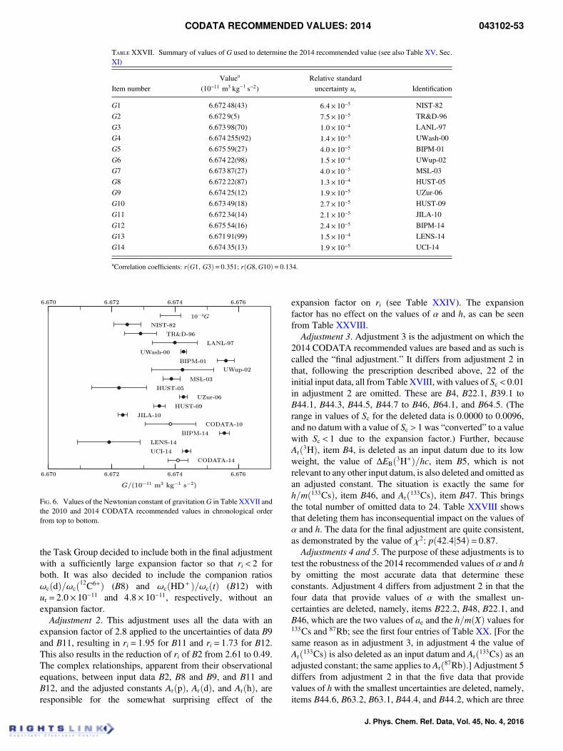
the Task Group decided to include both in the final adjustmentwith a sufficiently large expansion factor so that ri < 2 forboth. It was also decided to include the companion ratiosωcðdÞ=ωcð12C6+Þ (B8) and ωcðHD+ Þ=ωcðtÞ (B12) withur = 2:0× 10−11 and 4:8× 10⁻¹¹, respectively, without anexpansion factor.
Adjustment 2. This adjustment uses all the data with anexpansion factor of 2.8 applied to the uncertainties of data B9and B11, resulting in ri = 1:95 for B11 and ri = 1:73 for B12.This also results in the reduction of ri of B2 from 2.61 to 0.49.The complex relationships, apparent from their observationalequations, between input data B2, B8 and B9, and B11 andB12, and the adjusted constants ArðpÞ, ArðdÞ, and ArðhÞ, areresponsible for the somewhat surprising effect of the
expansion factor on ri (see Table XXIV). The expansionfactor has no effect on the values of α and h, as can be seenfrom Table XXVIII.
Adjustment 3. Adjustment 3 is the adjustment on which the2014 CODATA recommended values are based and as such iscalled the “final adjustment.” It differs from adjustment 2 inthat, following the prescription described above, 22 of theinitial input data, all from Table XVIII, with values of Sc < 0:01in adjustment 2 are omitted. These are B4, B22:1, B39:1 toB44:1, B44:3, B44:5, B44:7 to B46, B64:1, and B64:5. (Therange in values of Sc for the deleted data is 0.0000 to 0.0096,and no datum with a value of Sc > 1 was “converted” to a valuewith Sc < 1 due to the expansion factor.) Further, becauseArð3HÞ, item B4, is deleted as an input datum due to its lowweight, the value of ΔEBð3H+Þ=hc, item B5, which is notrelevant to any other input datum, is also deleted and omitted asan adjusted constant. The situation is exactly the same forh=mð133CsÞ, item B46, and Arð133CsÞ, item B47. This bringsthe total number of omitted data to 24. Table XXVIII showsthat deleting them has inconsequential impact on the values ofα and h. The data for the final adjustment are quite consistent,as demonstrated by the value of χ2: pð42:4j54Þ= 0:87.
Adjustments 4 and 5. The purpose of these adjustments is totest the robustness of the 2014 recommended values of α and hby omitting the most accurate data that determine theseconstants. Adjustment 4 differs from adjustment 2 in that thefour data that provide values of α with the smallest un-certainties are deleted, namely, items B22:2, B48, B22:1, andB46, which are the two values of ae and the h=mðXÞ values for133Cs and 87Rb; see the first four entries of Table XX. [For thesame reason as in adjustment 3, in adjustment 4 the value ofArð133CsÞ is also deleted as an input datum and Arð133CsÞ as anadjusted constant; the same applies to Arð87RbÞ.] Adjustment 5differs from adjustment 2 in that the five data that providevalues of h with the smallest uncertainties are deleted, namely,items B44:6, B63:2, B63:1, B44:4, and B44:2, which are three
TABLE XXVII. Summary of values of G used to determine the 2014 recommended value (see also Table XV, Sec.XI)
Item numberValuea
(10−11 m3 kg−1 s−2)Relative standarduncertainty ur Identification
G1 6.672 48(43) 6:4× 10⁻⁵ NIST-82
G2 6.672 9(5) 7:5× 10⁻⁵ TR&D-96
G3 6.673 98(70) 1:0× 10−4 LANL-97
G4 6.674 255(92) 1:4× 10⁻⁵ UWash-00
G5 6.675 59(27) 4:0× 10−5 BIPM-01
G6 6.674 22(98) 1:5× 10⁻⁴ UWup-02
G7 6.673 87(27) 4:0× 10−5 MSL-03
G8 6.672 22(87) 1:3× 10⁻⁴ HUST-05
G9 6.674 25(12) 1:9× 10⁻⁵ UZur-06
G10 6.673 49(18) 2:7× 10⁻⁵ HUST-09
G11 6.672 34(14) 2:1× 10⁻⁵ JILA-10
G12 6.675 54(16) 2:4× 10⁻⁵ BIPM-14
G13 6.671 91(99) 1:5× 10⁻⁴ LENS-14
G14 6.674 35(13) 1:9× 10⁻⁵ UCI-14
aCorrelation coefficients: rðG1, G3Þ= 0:351; rðG8,G10Þ= 0:134.
FIG. 6. Values of the Newtonian constant of gravitationG in Table XXVII andthe 2010 and 2014 CODATA recommended values in chronological orderfrom top to bottom.
CODATA RECOMMENDED VALUES: 2014 043102-53
J. Phys. Chem. Ref. Data, Vol. 45, No. 4, 2016
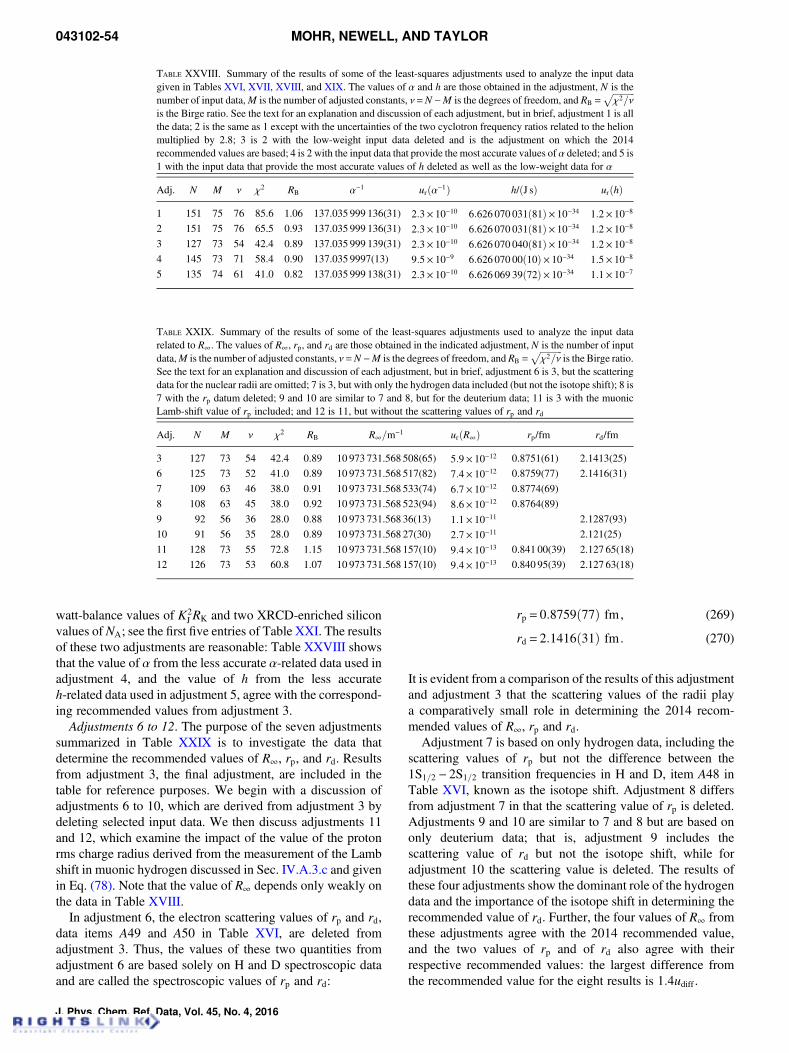
watt-balance values of K2J RK and two XRCD-enriched silicon
values of NA; see the first five entries of Table XXI. The resultsof these two adjustments are reasonable: Table XXVIII showsthat the value of α from the less accurate α-related data used inadjustment 4, and the value of h from the less accurateh-related data used in adjustment 5, agree with the correspond-ing recommended values from adjustment 3.
Adjustments 6 to 12. The purpose of the seven adjustmentssummarized in Table XXIX is to investigate the data thatdetermine the recommended values of R∞, rp, and rd. Resultsfrom adjustment 3, the final adjustment, are included in thetable for reference purposes. We begin with a discussion ofadjustments 6 to 10, which are derived from adjustment 3 bydeleting selected input data. We then discuss adjustments 11and 12, which examine the impact of the value of the protonrms charge radius derived from the measurement of the Lambshift in muonic hydrogen discussed in Sec. IV.A.3.c and givenin Eq. (78). Note that the value of R∞ depends only weakly onthe data in Table XVIII.
In adjustment 6, the electron scattering values of rp and rd,data items A49 and A50 in Table XVI, are deleted fromadjustment 3. Thus, the values of these two quantities fromadjustment 6 are based solely on H and D spectroscopic dataand are called the spectroscopic values of rp and rd:
rp = 0:8759ð77Þ fm, (269)
rd = 2:1416ð31Þ fm. (270)
It is evident from a comparison of the results of this adjustmentand adjustment 3 that the scattering values of the radii playa comparatively small role in determining the 2014 recom-mended values of R∞, rp and rd.
Adjustment 7 is based on only hydrogen data, including thescattering values of rp but not the difference between the1S1=2 − 2S1=2 transition frequencies in H and D, item A48 inTable XVI, known as the isotope shift. Adjustment 8 differsfrom adjustment 7 in that the scattering value of rp is deleted.Adjustments 9 and 10 are similar to 7 and 8 but are based ononly deuterium data; that is, adjustment 9 includes thescattering value of rd but not the isotope shift, while foradjustment 10 the scattering value is deleted. The results ofthese four adjustments show the dominant role of the hydrogendata and the importance of the isotope shift in determining therecommended value of rd. Further, the four values of R∞ fromthese adjustments agree with the 2014 recommended value,and the two values of rp and of rd also agree with theirrespective recommended values: the largest difference fromthe recommended value for the eight results is 1:4udiff .
TABLE XXVIII. Summary of the results of some of the least-squares adjustments used to analyze the input datagiven in Tables XVI, XVII, XVIII, and XIX. The values of α and h are those obtained in the adjustment, N is thenumber of input data,M is the number of adjusted constants, ν=N −M is the degrees of freedom, and RB =
ffiffiffiffiffiffiffiffiffiffiχ2=ν
pis the Birge ratio. See the text for an explanation and discussion of each adjustment, but in brief, adjustment 1 is allthe data; 2 is the same as 1 except with the uncertainties of the two cyclotron frequency ratios related to the helionmultiplied by 2.8; 3 is 2 with the low-weight input data deleted and is the adjustment on which the 2014recommended values are based; 4 is 2 with the input data that provide the most accurate values of α deleted; and 5 is1 with the input data that provide the most accurate values of h deleted as well as the low-weight data for α
Adj. N M ν χ2 RB α−1 urðα−1Þ h/ðJ sÞ urðhÞ
1 151 75 76 85.6 1.06 137.035 999 136(31) 2:3× 10⁻¹⁰ 6:626 070 031ð81Þ× 10−34 1:2× 10⁻⁸
2 151 75 76 65.5 0.93 137.035 999 136(31) 2:3× 10⁻¹⁰ 6:626 070 031ð81Þ× 10−34 1:2× 10⁻⁸
3 127 73 54 42.4 0.89 137.035 999 139(31) 2:3× 10⁻¹⁰ 6:626 070 040ð81Þ× 10−34 1:2× 10⁻⁸
4 145 73 71 58.4 0.90 137.035 9997(13) 9:5× 10⁻⁹ 6:626 070 00ð10Þ× 10−34 1:5× 10⁻⁸
5 135 74 61 41.0 0.82 137.035 999 138(31) 2:3× 10⁻¹⁰ 6:626 069 39ð72Þ× 10−34 1:1× 10⁻⁷
TABLE XXIX. Summary of the results of some of the least-squares adjustments used to analyze the input datarelated to R∞. The values of R∞, rp, and rd are those obtained in the indicated adjustment, N is the number of inputdata,M is the number of adjusted constants, ν=N −M is the degrees of freedom, and RB =
ffiffiffiffiffiffiffiffiffiffiχ2=ν
pis the Birge ratio.
See the text for an explanation and discussion of each adjustment, but in brief, adjustment 6 is 3, but the scatteringdata for the nuclear radii are omitted; 7 is 3, but with only the hydrogen data included (but not the isotope shift); 8 is7 with the rp datum deleted; 9 and 10 are similar to 7 and 8, but for the deuterium data; 11 is 3 with the muonicLamb-shift value of rp included; and 12 is 11, but without the scattering values of rp and rd
Adj. N M ν χ2 RB R∞=m−1 urðR∞Þ rp/fm rd/fm
3 127 73 54 42.4 0.89 10 973 731.568 508(65) 5:9× 10⁻¹² 0.8751(61) 2.1413(25)
6 125 73 52 41.0 0.89 10 973 731.568 517(82) 7:4× 10⁻¹² 0.8759(77) 2.1416(31)
7 109 63 46 38.0 0.91 10 973 731.568 533(74) 6:7× 10⁻¹² 0.8774(69)
8 108 63 45 38.0 0.92 10 973 731.568 523(94) 8:6× 10⁻¹² 0.8764(89)
9 92 56 36 28.0 0.88 10 973 731.568 36(13) 1:1× 10⁻¹¹ 2.1287(93)
10 91 56 35 28.0 0.89 10 973 731.568 27(30) 2:7× 10⁻¹¹ 2.121(25)
11 128 73 55 72.8 1.15 10 973 731.568 157(10) 9:4× 10⁻¹³ 0.841 00(39) 2.127 65(18)
12 126 73 53 60.8 1.07 10 973 731.568 157(10) 9:4× 10⁻¹³ 0.840 95(39) 2.127 63(18)
043102-54 MOHR, NEWELL, AND TAYLOR
J. Phys. Chem. Ref. Data, Vol. 45, No. 4, 2016
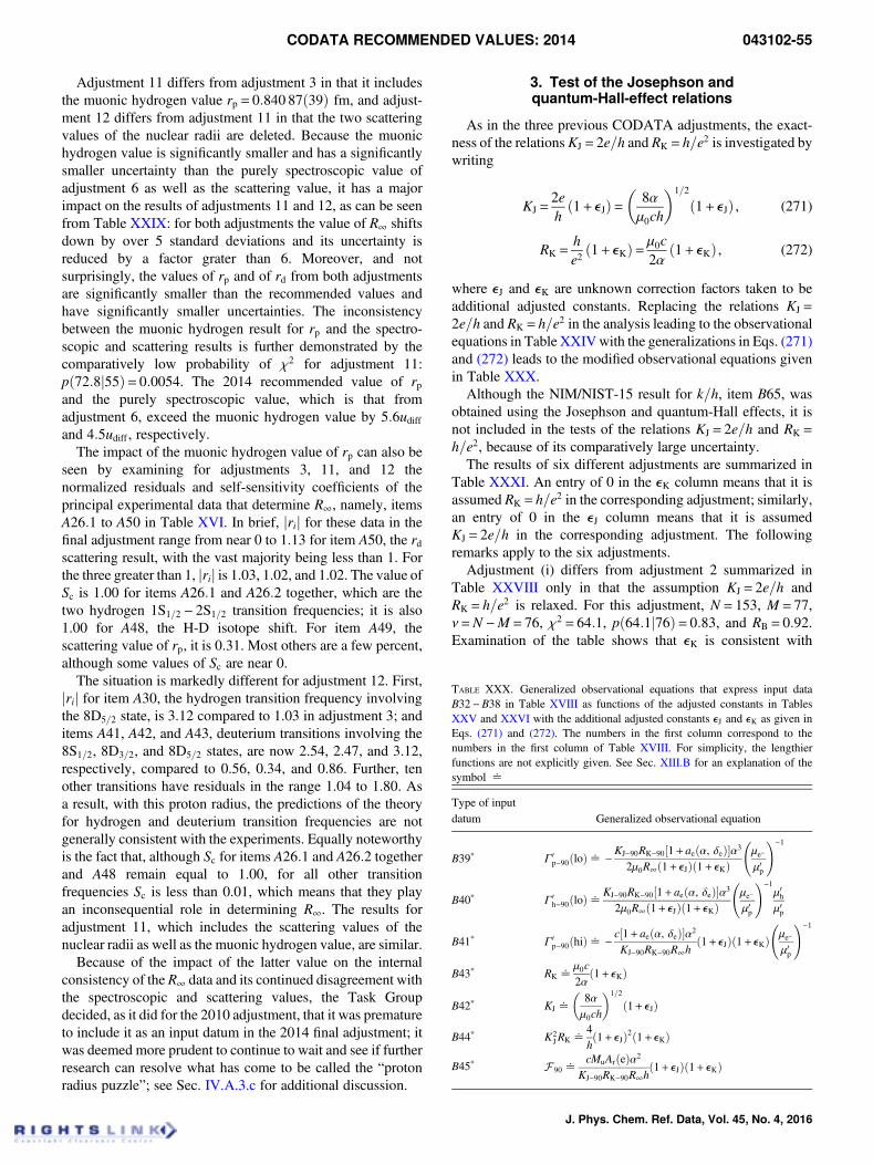
Adjustment 11 differs from adjustment 3 in that it includesthe muonic hydrogen value rp = 0:840 87ð39Þ fm, and adjust-ment 12 differs from adjustment 11 in that the two scatteringvalues of the nuclear radii are deleted. Because the muonichydrogen value is significantly smaller and has a significantlysmaller uncertainty than the purely spectroscopic value ofadjustment 6 as well as the scattering value, it has a majorimpact on the results of adjustments 11 and 12, as can be seenfrom Table XXIX: for both adjustments the value of R∞ shiftsdown by over 5 standard deviations and its uncertainty isreduced by a factor grater than 6. Moreover, and notsurprisingly, the values of rp and of rd from both adjustmentsare significantly smaller than the recommended values andhave significantly smaller uncertainties. The inconsistencybetween the muonic hydrogen result for rp and the spectro-scopic and scattering results is further demonstrated by thecomparatively low probability of χ2 for adjustment 11:pð72:8j55Þ= 0:0054. The 2014 recommended value of rpand the purely spectroscopic value, which is that fromadjustment 6, exceed the muonic hydrogen value by 5:6udiffand 4:5udiff , respectively.
The impact of the muonic hydrogen value of rp can also beseen by examining for adjustments 3, 11, and 12 thenormalized residuals and self-sensitivity coefficients of theprincipal experimental data that determine R∞, namely, itemsA26:1 to A50 in Table XVI. In brief, jrij for these data in thefinal adjustment range from near 0 to 1.13 for item A50, the rdscattering result, with the vast majority being less than 1. Forthe three greater than 1, jrij is 1.03, 1.02, and 1.02. The value ofSc is 1.00 for items A26:1 and A26:2 together, which are thetwo hydrogen 1S1=2 − 2S1=2 transition frequencies; it is also1.00 for A48, the H-D isotope shift. For item A49, thescattering value of rp, it is 0.31. Most others are a few percent,although some values of Sc are near 0.
The situation is markedly different for adjustment 12. First,jrij for item A30, the hydrogen transition frequency involvingthe 8D5=2 state, is 3.12 compared to 1.03 in adjustment 3; anditems A41, A42, and A43, deuterium transitions involving the8S1=2, 8D3=2, and 8D5=2 states, are now 2.54, 2.47, and 3.12,respectively, compared to 0.56, 0.34, and 0.86. Further, tenother transitions have residuals in the range 1.04 to 1.80. Asa result, with this proton radius, the predictions of the theoryfor hydrogen and deuterium transition frequencies are notgenerally consistent with the experiments. Equally noteworthyis the fact that, although Sc for items A26:1 and A26:2 togetherand A48 remain equal to 1.00, for all other transitionfrequencies Sc is less than 0.01, which means that they playan inconsequential role in determining R∞. The results foradjustment 11, which includes the scattering values of thenuclear radii as well as the muonic hydrogen value, are similar.
Because of the impact of the latter value on the internalconsistency of the R∞ data and its continued disagreement withthe spectroscopic and scattering values, the Task Groupdecided, as it did for the 2010 adjustment, that it was prematureto include it as an input datum in the 2014 final adjustment; itwas deemed more prudent to continue to wait and see if furtherresearch can resolve what has come to be called the “protonradius puzzle”; see Sec. IV.A.3.c for additional discussion.
3. Test of the Josephson andquantum-Hall-effect relations
As in the three previous CODATA adjustments, the exact-ness of the relations KJ = 2e=h and RK = h=e2 is investigated bywriting
KJ =2ehð1+ eJÞ=
8αμ0ch
�1=2
ð1+ eJÞ , (271)
RK =he2ð1+ eKÞ= μ0c
2αð1+ eKÞ , (272)
where eJ and eK are unknown correction factors taken to beadditional adjusted constants. Replacing the relations KJ =
2e=h and RK = h=e2 in the analysis leading to the observationalequations in Table XXIVwith the generalizations in Eqs. (271)and (272) leads to the modified observational equations givenin Table XXX.
Although the NIM/NIST-15 result for k=h, item B65, wasobtained using the Josephson and quantum-Hall effects, it isnot included in the tests of the relations KJ = 2e=h and RK =
h=e2, because of its comparatively large uncertainty.The results of six different adjustments are summarized in
Table XXXI. An entry of 0 in the eK column means that it isassumed RK = h=e2 in the corresponding adjustment; similarly,an entry of 0 in the eJ column means that it is assumedKJ = 2e=h in the corresponding adjustment. The followingremarks apply to the six adjustments.
Adjustment (i) differs from adjustment 2 summarized inTable XXVIII only in that the assumption KJ = 2e=h andRK = h=e2 is relaxed. For this adjustment, N = 153, M = 77,ν=N −M = 76, χ2 = 64:1, pð64:1j76Þ= 0:83, and RB = 0:92.Examination of the table shows that eK is consistent with
TABLE XXX. Generalized observational equations that express input dataB32−B38 in Table XVIII as functions of the adjusted constants in TablesXXV and XXVI with the additional adjusted constants eJ and eK as given inEqs. (271) and (272). The numbers in the first column correspond to thenumbers in the first column of Table XVIII. For simplicity, the lengthierfunctions are not explicitly given. See Sec. XIII.B for an explanation of thesymbol ^
Type of inputdatum Generalized observational equation
B39* Γ0p−90ðloÞ^ −KJ−90RK−90½1+ aeðα, δeÞ�α3
2μ0R∞ð1+ eJÞð1+ eKÞ
μe−
μ0p
!−1
B40* Γ0h−90ðloÞ^
KJ−90RK−90½1+ aeðα, δeÞ�α3
2μ0R∞ð1+ eJÞð1+ eKÞ
μe−
μ0p
!−1μ0hμ0p
B41* Γ0p−90ðhiÞ^ − c½1+ aeðα, δeÞ�α2
KJ−90RK−90R∞hð1+ eJÞð1+ eKÞ
μe−
μ0p
!−1
B43* RK ^μ0c2α
ð1+ eKÞ
B42* KJ ^
8αμ0ch
�1=2
ð1+ eJÞ
B44* K2JRK ^
4hð1+ eJÞ2ð1+ eKÞ
B45* F 90 ^cMuArðeÞα2
KJ−90RK−90R∞hð1+ eJÞð1+ eKÞ
CODATA RECOMMENDED VALUES: 2014 043102-55
J. Phys. Chem. Ref. Data, Vol. 45, No. 4, 2016
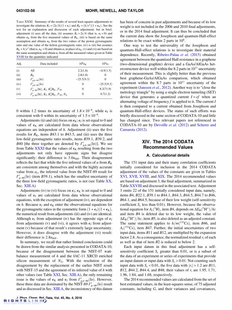
0 within 1.2 times its uncertainty of 1:8× 10⁻⁸, while eJ isconsistent with 0 within its uncertainty of 1:5× 10⁻⁸.
Adjustments (ii) and (iii) focus on eK; eJ is set equal to 0 andvalues of eK are calculated from data whose observationalequations are independent of h. Adjustment (ii) uses the fiveresults for RK, items B43:1 to B43:5, and (iii) uses the threelow-field gyromagnetic ratio results, items B39:1, B39:2, andB40 [the three together are denoted by Γ0
p,h−90ðloÞ]. We seefrom Table XXXI that the values of eK resulting from the twoadjustments not only have opposite signs but disagreesignificantly: their difference is 3:0udiff . Their disagreementreflects the fact that while the five inferred values of α from RK
are consistent among themselves and with the highly accuratevalue from ae, the inferred value from the NIST-89 result forΓ0p−90ðloÞ (item B39:1), which has the smallest uncertainty of
the three low-field gyromagnetic ratios, is not (see Table XX,Sec. XIII.A)
Adjustments (iv) to (vi) focus on eJ; eK is set equal to 0 andvalues of eJ are calculated from data whose observationalequations, with the exception of adjustment (iv), are dependenton h. Because eJ and eK enter the observational equations forthe gyromagnetic ratios in the symmetric form ð1+ eJÞð1+ eKÞ,the numerical result from adjustments (iii) and (iv) are identical.Although eJ from adjustment (iv) has the opposite sign of eJfrom adjustments (v) and (vi), it agrees with eJ from adjust-ment (v) because of that result’s extremely large uncertainty.However, it does disagree with the adjustment (vi) result:their difference is 2:8udiff .
In summary, we recall that rather limited conclusions couldbe drawn from the similar analysis presented in CODATA-10,because of the disagreement between the NIST-07 watt-balance measurement of h and the IAC-11 XRCD enrichedsilicon measurement of NA. With the resolution of thedisagreement by the replacement of the earlier NIST resultwith NIST-15 and the agreement of its inferred value of h withother values (see Table XXI, Sec. XIII.A), the only remainingissue is the values of eK and eJ from Γ0
p,h−90ðloÞ. However,these three data are dominated by the NIST-89 Γ0
p−90ðloÞ resultand as discussed in Sec. XIII.A, the inconsistency of this datum
has been of concern in past adjustments and because of its lowweight is not included in the 2006 and 2010 final adjustments,or in the 2014 final adjustment. It can thus be concluded thatthe current data show the Josephson and quantum-Hall-effectrelations to be exact within 2 parts in 108.
One way to test the universality of the Josephson andquantum-Hall-effect relations is to investigate their materialdependence. Recently, Ribeiro-Palau et al. (2015) obtainedagreement between the quantized Hall resistance in a graphene(two-dimensional graphite) device and a GaAs/AlGaAs het-erostructure device well within the 8.2 parts in 1011 uncertaintyof their measurement. This is slightly better than the previousbest graphene-GaAs/AlGaAs comparison, which obtainedagreement within the 8.7 parts in 1011 uncertainty of theexperiment (Janssen et al., 2012). Another way is to “close themetrology triangle” by using a single electron tunneling (SET)device that generates a quantized current I = ef when analternating voltage of frequency f is applied to it. The current Iis then compared to a current obtained from Josephson andquantum-Hall-effect devices. The status of such efforts wasbriefly discussed in the same section of CODATA-10 and littlehas changed since. Two relevant papers not referenced inCODATA-10 are by Devoille et al. (2012) and Scherer andCamarota (2012).
XIV. The 2014 CODATARecommended Values
A. Calculational details
The 151 input data and their many correlation coefficientsinitially considered for inclusion in the 2014 CODATAadjustment of the values of the constants are given in TablesXVI, XVII, XVIII, and XIX. The 2014 recommended valuesare based on adjustment 3, the final adjustment, summarized inTable XXVIII and discussed in the associated text. Adjustment3 omits 22 of the 151 initially considered input data, namely,items B4, B22:1, B39:1 to B44:1, B44:3, B44:5, B44:7 to B46,B64:1, and B64:5, because of their low weight (self-sensitivitycoefficient Sc less than 0.01). However, because the observa-tional equation for Arð3HÞ, item B4, depends on ΔEBð3H+Þ=hcand item B4 is deleted due to its low weight, the value ofΔEBð3H+Þ=hc, item B5, is also deleted as an adjusted constant.The same statement applies to h=mð133CsÞ, item B46, andArð133CsÞ, item B47. Further, the initial uncertainties of twoinput data, items B11 and B12, are multiplied by the expansionfactor 2.8. As a consequence, the normalized residual ri of eachas well as that of item B2 is reduced to below 2.
Each input datum in this final adjustment has a self-sensitivity coefficient Sc greater than 0.01, or is a subset ofthe data of an experiment or series of experiments that providean input datum or input data with Sc > 0:01. Not counting suchinput data with Sc < 0:01, the five data with jrij> 1:2 are B11,B12, B44:2, B44:4, and B48; their values of ri are 1.95, 1.71,1.96, 1.84, and 1.68, respectively.
The 2014 recommended values are calculated from the set ofbest estimated values, in the least-squares sense, of 75 adjustedconstants, including G, and their variances and covariances,
TABLE XXXI. Summary of the results of several least-squares adjustments toinvestigate the relations KJ = ð2e=hÞð1+ eJÞ and RK = ðh=e2Þð1+ eKÞ. See thetext for an explanation and discussion of each adjustment, but in brief,adjustment (i) uses all the data, (ii) assumes KJ = 2e=h (that is, eJ = 0) andobtains eK from the five measured values of RK, (iii) is based on the sameassumption and obtains eK from the two values of the proton gyromagneticratio and one value of the helion gyromagnetic ratio, (iv) is (iii) but assumesRK = h=e2 (that is, eK = 0) and obtains eJ in place of eK, (v) and (vi) are based onthe same assumption and obtain eJ from all the measured values given in TableXVIII for the quantities indicated
Adj. Data included 108eK 108eJ
(i) All 2.2(1.8) −0:9ð1:5Þ(ii) RK 2.8(1.8) 0(iii) Γ0
p,h−90ðloÞ −25:5ð9:3Þ 0
(iv) Γ0p,h−90ðloÞ 0 −25:5ð9:3Þ
(v) Γ0p−90ðhiÞ, KJ, K2
JRK, F 90 0 8.2(71.9)
(vi) Γ0p−90ðhiÞ, KJ, K2
JRK, F 90, NA 0 0.7(1.2)
043102-56 MOHR, NEWELL, AND TAYLOR
J. Phys. Chem. Ref. Data, Vol. 45, No. 4, 2016
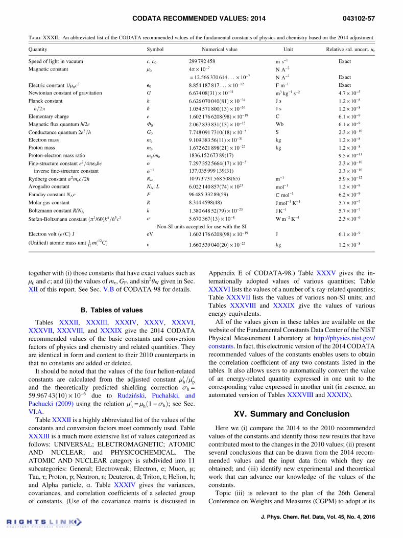
together with (i) those constants that have exact values such asμ0 and c; and (ii) the values ofmτ,GF, and sin
2θW given in Sec.XII of this report. See Sec. V.B of CODATA-98 for details.
B. Tables of values
Tables XXXII, XXXIII, XXXIV, XXXV, XXXVI,XXXVII, XXXVIII, and XXXIX give the 2014 CODATArecommended values of the basic constants and conversionfactors of physics and chemistry and related quantities. Theyare identical in form and content to their 2010 counterparts inthat no constants are added or deleted.
It should be noted that the values of the four helion-relatedconstants are calculated from the adjusted constant μ0h=μ
0p
and the theoretically predicted shielding correction σh =
59:967 43ð10Þ× 10−6 due to Rudzinski, Puchalski, andPachucki (2009) using the relation μ0h = μhð1−σhÞ; see Sec.VI.A.
Table XXXII is a highly abbreviated list of the values of theconstants and conversion factors most commonly used. TableXXXIII is a much more extensive list of values categorized asfollows: UNIVERSAL; ELECTROMAGNETIC; ATOMICAND NUCLEAR; and PHYSICOCHEMICAL. TheATOMIC AND NUCLEAR category is subdivided into 11subcategories: General; Electroweak; Electron, e; Muon, μ;Tau, τ; Proton, p; Neutron, n; Deuteron, d; Triton, t; Helion, h;and Alpha particle, α. Table XXXIV gives the variances,covariances, and correlation coefficients of a selected groupof constants. (Use of the covariance matrix is discussed in
Appendix E of CODATA-98.) Table XXXV gives the in-ternationally adopted values of various quantities; TableXXXVI lists the values of a number of x-ray-related quantities;Table XXXVII lists the values of various non-SI units; andTables XXXVIII and XXXIX give the values of variousenergy equivalents.
All of the values given in these tables are available on thewebsite of the Fundamental Constants Data Center of the NISTPhysical Measurement Laboratory at http://physics.nist.gov/constants. In fact, this electronic version of the 2014 CODATArecommended values of the constants enables users to obtainthe correlation coefficient of any two constants listed in thetables. It also allows users to automatically convert the valueof an energy-related quantity expressed in one unit to thecorresponding value expressed in another unit (in essence, anautomated version of Tables XXXVIII and XXXIX).
XV. Summary and Conclusion
Here we (i) compare the 2014 to the 2010 recommendedvalues of the constants and identify those new results that havecontributed most to the changes in the 2010 values; (ii) presentseveral conclusions that can be drawn from the 2014 recom-mended values and the input data from which they areobtained; and (iii) identify new experimental and theoreticalwork that can advance our knowledge of the values of theconstants.
Topic (iii) is relevant to the plan of the 26th GeneralConference on Weights and Measures (CGPM) to adopt at its
TABLE XXXII. An abbreviated list of the CODATA recommended values of the fundamental constants of physics and chemistry based on the 2014 adjustment
Quantity Symbol Numerical value Unit Relative std. uncert. ur
Speed of light in vacuum c, c0 299 792 458 m s−1 Exact
Magnetic constant μ0 4π× 10−7 N A−2
= 12:566 370 614 . . . × 10−7 N A−2 Exact
Electric constant 1/μ0c2 e0 8:854 187 817 . . . × 10−12 F m−1 Exact
Newtonian constant of gravitation G 6:674 08ð31Þ× 10−11 m3 kg−1 s−2 4:7× 10⁻⁵
Planck constant h 6:626 070 040ð81Þ× 10−34 J s 1:2× 10⁻⁸
h=2π ℏ 1:054 571 800ð13Þ× 10−34 J s 1:2× 10⁻⁸
Elementary charge e 1:602 176 6208ð98Þ× 10−19 C 6:1× 10⁻⁹
Magnetic flux quantum h/2e Φ0 2:067 833 831ð13Þ× 10−15 Wb 6:1× 10⁻⁹
Conductance quantum 2e2=h G0 7:748 091 7310ð18Þ× 10−5 S 2:3× 10⁻¹⁰
Electron mass me 9:109 383 56ð11Þ× 10−31 kg 1:2× 10⁻⁸
Proton mass mp 1:672 621 898ð21Þ× 10−27 kg 1:2× 10⁻⁸
Proton-electron mass ratio mp/me 1836.152 673 89(17) 9:5× 10⁻¹¹
Fine-structure constant e2=4πe0ℏc α 7:297 352 5664ð17Þ× 10−3 2:3× 10⁻¹⁰
inverse fine-structure constant α−1 137.035 999 139(31) 2:3× 10⁻¹⁰
Rydberg constant α2mec=2h R∞ 10 973 731.568 508(65) m−1 5:9× 10⁻¹²
Avogadro constant NA, L 6:022 140 857ð74Þ× 1023 mol−1 1:2× 10⁻⁸
Faraday constant NAe F 96 485.332 89(59) C mol−1 6:2× 10⁻⁹
Molar gas constant R 8.314 4598(48) Jmol−1 K−1 5:7× 10⁻⁷
Boltzmann constant R/NA k 1:380 648 52ð79Þ× 10−23 J K−1 5:7× 10⁻⁷
Stefan-Boltzmann constant ðπ2/60Þk4=ℏ3c2 σ 5:670 367ð13Þ× 10−8 Wm−2 K−4 2:3× 10⁻⁶
Non-SI units accepted for use with the SIElectron volt ðe /CÞ J eV 1:602 176 6208ð98Þ× 10−19 J 6:1× 10⁻⁹
(Unified) atomic mass unit 112mð12CÞ u 1:660 539 040ð20Þ× 10−27 kg 1:2× 10⁻⁸
CODATA RECOMMENDED VALUES: 2014 043102-57
J. Phys. Chem. Ref. Data, Vol. 45, No. 4, 2016
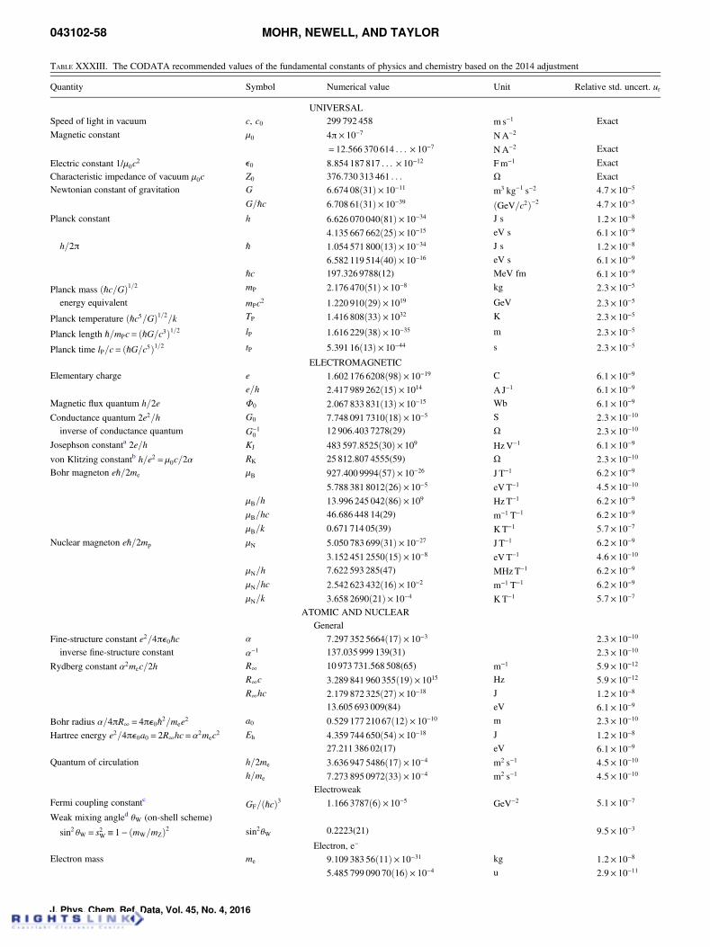
TABLE XXXIII. The CODATA recommended values of the fundamental constants of physics and chemistry based on the 2014 adjustment
Quantity Symbol Numerical value Unit Relative std. uncert. ur
UNIVERSALSpeed of light in vacuum c, c0 299 792 458 m s−1 Exact
Magnetic constant μ0 4π× 10−7 NA−2
= 12:566 370 614 . . . × 10−7 NA−2 Exact
Electric constant 1/μ0c2 e0 8:854 187 817 . . . × 10−12 Fm−1 Exact
Characteristic impedance of vacuum μ0c Z0 376:730 313 461 . . . Ω ExactNewtonian constant of gravitation G 6:674 08ð31Þ× 10−11 m3 kg−1 s−2 4:7× 10⁻⁵
G=ℏc 6:708 61ð31Þ× 10−39 ðGeV=c2Þ−2 4:7× 10⁻⁵
Planck constant h 6:626 070 040ð81Þ× 10−34 J s 1:2× 10⁻⁸
4:135 667 662ð25Þ× 10−15 eV s 6:1× 10⁻⁹
h=2π ℏ 1:054 571 800ð13Þ× 10−34 J s 1:2× 10⁻⁸
6:582 119 514ð40Þ× 10−16 eV s 6:1× 10⁻⁹
ℏc 197.326 9788(12) MeV fm 6:1× 10⁻⁹
Planck mass ðℏc=GÞ1=2 mP 2:176 470ð51Þ× 10−8 kg 2:3× 10⁻⁵
energy equivalent mPc2 1:220 910ð29Þ× 1019 GeV 2:3× 10⁻⁵
Planck temperature ðℏc5=GÞ1=2=k TP 1:416 808ð33Þ× 1032 K 2:3× 10⁻⁵
Planck length ℏ=mPc= ðℏG=c3Þ1=2 lP 1:616 229ð38Þ× 10−35 m 2:3× 10⁻⁵
Planck time lP=c= ðℏG=c5Þ1=2 tP 5:391 16ð13Þ× 10−44 s 2:3× 10⁻⁵
ELECTROMAGNETICElementary charge e 1:602 176 6208ð98Þ× 10−19 C 6:1× 10⁻⁹
e=h 2:417 989 262ð15Þ× 1014 A J−1 6:1× 10⁻⁹
Magnetic flux quantum h=2e Φ0 2:067 833 831ð13Þ× 10−15 Wb 6:1× 10⁻⁹
Conductance quantum 2e2=h G0 7:748 091 7310ð18Þ× 10−5 S 2:3× 10⁻¹⁰
inverse of conductance quantum G−10 12 906.403 7278(29) Ω 2:3× 10⁻¹⁰
Josephson constanta 2e=h KJ 483 597:8525ð30Þ× 109 HzV−1 6:1× 10⁻⁹
von Klitzing constantb h=e2 = μ0c=2α RK 25 812.807 4555(59) Ω 2:3× 10⁻¹⁰
Bohr magneton eℏ=2me μB 927:400 9994ð57Þ× 10−26 J T−1 6:2× 10⁻⁹
5:788 381 8012ð26Þ× 10−5 eVT−1 4:5× 10⁻¹⁰
μB=h 13:996 245 042ð86Þ× 109 Hz T−1 6:2× 10⁻⁹
μB=hc 46.686 448 14(29) m−1 T−1 6:2× 10⁻⁹
μB=k 0.671 714 05(39) KT−1 5:7× 10⁻⁷
Nuclear magneton eℏ=2mp μN 5:050 783 699ð31Þ× 10−27 J T−1 6:2× 10⁻⁹
3:152 451 2550ð15Þ× 10−8 eVT−1 4:6× 10⁻¹⁰
μN=h 7.622 593 285(47) MHzT−1 6:2× 10⁻⁹
μN=hc 2:542 623 432ð16Þ× 10−2 m−1 T−1 6:2× 10⁻⁹
μN=k 3:658 2690ð21Þ× 10−4 K T−1 5:7× 10⁻⁷
ATOMIC AND NUCLEARGeneral
Fine-structure constant e2=4πe0ℏc α 7:297 352 5664ð17Þ× 10−3 2:3× 10⁻¹⁰
inverse fine-structure constant α−1 137.035 999 139(31) 2:3× 10⁻¹⁰
Rydberg constant α2mec=2h R∞ 10 973 731.568 508(65) m−1 5:9× 10⁻¹²
R∞c 3:289 841 960 355ð19Þ× 1015 Hz 5:9× 10⁻¹²
R∞hc 2:179 872 325ð27Þ× 10−18 J 1:2× 10⁻⁸
13.605 693 009(84) eV 6:1× 10⁻⁹
Bohr radius α=4πR∞ = 4πe0ℏ2=mee2 a0 0:529 177 210 67ð12Þ× 10−10 m 2:3× 10⁻¹⁰
Hartree energy e2=4πe0a0 = 2R∞hc=α2mec2 Eh 4:359 744 650ð54Þ× 10−18 J 1:2× 10⁻⁸
27.211 386 02(17) eV 6:1× 10⁻⁹
Quantum of circulation h=2me 3:636 947 5486ð17Þ× 10−4 m2 s−1 4:5× 10⁻¹⁰
h=me 7:273 895 0972ð33Þ× 10−4 m2 s−1 4:5× 10⁻¹⁰
ElectroweakFermi coupling constantc GF=ðℏcÞ3 1:166 3787ð6Þ× 10−5 GeV−2 5:1× 10⁻⁷
Weak mixing angled θW (on-shell scheme)
sin2 θW = s2W ≡ 1− ðmW=mZÞ2 sin2θW 0.2223(21) 9:5× 10⁻³
Electron, e−
Electron mass me 9:109 383 56ð11Þ× 10−31 kg 1:2× 10⁻⁸
5:485 799 090 70ð16Þ× 10−4 u 2:9× 10⁻¹¹
043102-58 MOHR, NEWELL, AND TAYLOR
J. Phys. Chem. Ref. Data, Vol. 45, No. 4, 2016
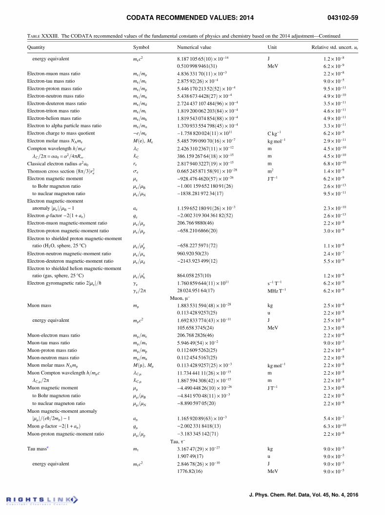
TABLE XXXIII. The CODATA recommended values of the fundamental constants of physics and chemistry based on the 2014 adjustment—Continued
Quantity Symbol Numerical value Unit Relative std. uncert. ur
energy equivalent mec2 8:187 105 65ð10Þ× 10−14 J 1:2× 10⁻⁸
0.510 998 9461(31) MeV 6:2× 10⁻⁹
Electron-muon mass ratio me=mμ 4:836 331 70ð11Þ× 10−3 2:2× 10⁻⁸
Electron-tau mass ratio me=mτ 2:875 92ð26Þ× 10−4 9:0× 10−5
Electron-proton mass ratio me=mp 5:446 170 213 52ð52Þ× 10−4 9:5× 10⁻¹¹
Electron-neutron mass ratio me=mn 5:438 673 4428ð27Þ× 10−4 4:9× 10⁻¹⁰
Electron-deuteron mass ratio me=md 2:724 437 107 484ð96Þ× 10−4 3:5× 10⁻¹¹
Electron-triton mass ratio me=mt 1:819 200 062 203ð84Þ× 10−4 4:6× 10⁻¹¹
Electron-helion mass ratio me=mh 1:819 543 074 854ð88Þ× 10−4 4:9× 10⁻¹¹
Electron to alpha particle mass ratio me=mα 1:370 933 554 798ð45Þ× 10−4 3:3× 10⁻¹¹
Electron charge to mass quotient −e=me −1:758 820 024ð11Þ× 1011 C kg−1 6:2× 10⁻⁹
Electron molar mass NAme MðeÞ, Me 5:485 799 090 70ð16Þ× 10−7 kgmol−1 2:9× 10⁻¹¹
Compton wavelength h=mec λC 2:426 310 2367ð11Þ× 10−12 m 4:5× 10⁻¹⁰
λC=2π=αa0 =α2=4πR∞ ƛC 386:159 267 64ð18Þ× 10−15 m 4:5× 10⁻¹⁰
Classical electron radius α2a0 re 2:817 940 3227ð19Þ× 10−15 m 6:8× 10⁻¹⁰
Thomson cross section ð8π=3Þr2e σe 0:665 245 871 58ð91Þ× 10−28 m2 1:4× 10⁻⁹
Electron magnetic moment μe −928:476 4620ð57Þ× 10−26 J T−1 6:2× 10⁻⁹
to Bohr magneton ratio μe=μB −1:001 159 652 180 91ð26Þ 2:6× 10⁻¹³
to nuclear magneton ratio μe=μN −1838:281 972 34ð17Þ 9:5× 10⁻¹¹
Electron magnetic-momentanomaly jμej=μB − 1 ae 1:159 652 180 91ð26Þ× 10−3 2:3× 10⁻¹⁰
Electron g-factor −2ð1+ aeÞ ge −2:002 319 304 361 82ð52Þ 2:6× 10⁻¹³
Electron-muon magnetic-moment ratio μe=μμ 206.766 9880(46) 2:2× 10⁻⁸
Electron-proton magnetic-moment ratio μe=μp −658:210 6866ð20Þ 3:0× 10−9
Electron to shielded proton magnetic-momentratio (H2O, sphere, 25 °C) μe=μ
0p −658:227 5971ð72Þ 1:1× 10⁻⁸
Electron-neutron magnetic-moment ratio μe=μn 960.920 50(23) 2:4× 10⁻⁷
Electron-deuteron magnetic-moment ratio μe=μd −2143:923 499ð12Þ 5:5× 10⁻⁹
Electron to shielded helion magnetic-momentratio (gas, sphere, 25 °C) μe=μ
0h 864.058 257(10) 1:2× 10⁻⁸
Electron gyromagnetic ratio 2jμej=ℏ γe 1:760 859 644ð11Þ× 1011 s−1 T−1 6:2× 10⁻⁹
γe=2π 28 024.951 64(17) MHzT−1 6:2× 10⁻⁹
Muon, μ−
Muon mass mμ 1:883 531 594ð48Þ× 10−28 kg 2:5× 10⁻⁸
0.113 428 9257(25) u 2:2× 10⁻⁸
energy equivalent mμc2 1:692 833 774ð43Þ× 10−11 J 2:5× 10⁻⁸
105.658 3745(24) MeV 2:3× 10⁻⁸
Muon-electron mass ratio mμ=me 206.768 2826(46) 2:2× 10⁻⁸
Muon-tau mass ratio mμ=mτ 5:946 49ð54Þ× 10−2 9:0× 10−5
Muon-proton mass ratio mμ=mp 0.112 609 5262(25) 2:2× 10⁻⁸
Muon-neutron mass ratio mμ=mn 0.112 454 5167(25) 2:2× 10⁻⁸
Muon molar mass NAmμ MðμÞ, Mμ 0:113 428 9257ð25Þ× 10−3 kgmol−1 2:2× 10⁻⁸
Muon Compton wavelength h=mμc λC,μ 11:734 441 11ð26Þ× 10−15 m 2:2× 10⁻⁸
λC,μ=2π ƛC,μ 1:867 594 308ð42Þ× 10−15 m 2:2× 10⁻⁸
Muon magnetic moment μμ −4:490 448 26ð10Þ× 10−26 J T−1 2:3× 10⁻⁸
to Bohr magneton ratio μμ=μB −4:841 970 48ð11Þ× 10−3 2:2× 10⁻⁸
to nuclear magneton ratio μμ=μN −8:890 597 05ð20Þ 2:2× 10⁻⁸
Muon magnetic-moment anomalyjμμj=ðeℏ=2mμÞ− 1 aμ 1:165 920 89ð63Þ× 10−3 5:4× 10⁻⁷
Muon g-factor −2ð1+ aμÞ gμ −2:002 331 8418ð13Þ 6:3× 10⁻¹⁰
Muon-proton magnetic-moment ratio μμ=μp −3:183 345 142ð71Þ 2:2× 10⁻⁸
Tau, τ−
Tau masse mτ 3:167 47ð29Þ× 10−27 kg 9:0× 10−5
1.907 49(17) u 9:0× 10−5
energy equivalent mτc2 2:846 78ð26Þ× 10−10 J 9:0× 10−5
1776.82(16) MeV 9:0× 10−5
CODATA RECOMMENDED VALUES: 2014 043102-59
J. Phys. Chem. Ref. Data, Vol. 45, No. 4, 2016
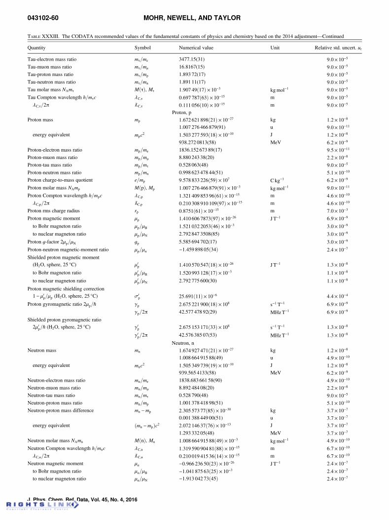
TABLE XXXIII. The CODATA recommended values of the fundamental constants of physics and chemistry based on the 2014 adjustment—Continued
Quantity Symbol Numerical value Unit Relative std. uncert. ur
Tau-electron mass ratio mτ=me 3477.15(31) 9:0× 10−5
Tau-muon mass ratio mτ=mμ 16.8167(15) 9:0× 10−5
Tau-proton mass ratio mτ=mp 1.893 72(17) 9:0× 10−5
Tau-neutron mass ratio mτ=mn 1.891 11(17) 9:0× 10−5
Tau molar mass NAmτ MðτÞ, Mτ 1:907 49ð17Þ× 10−3 kgmol−1 9:0× 10−5
Tau Compton wavelength h=mτc λC,τ 0:697 787ð63Þ× 10−15 m 9:0× 10−5
λC,τ=2π ƛC,τ 0:111 056ð10Þ× 10−15 m 9:0× 10−5
Proton, pProton mass mp 1:672 621 898ð21Þ× 10−27 kg 1:2× 10⁻⁸
1.007 276 466 879(91) u 9:0× 10−11
energy equivalent mpc2 1:503 277 593ð18Þ× 10−10 J 1:2× 10⁻⁸
938.272 0813(58) MeV 6:2× 10⁻⁹
Proton-electron mass ratio mp=me 1836.152 673 89(17) 9:5× 10⁻¹¹
Proton-muon mass ratio mp=mμ 8.880 243 38(20) 2:2× 10⁻⁸
Proton-tau mass ratio mp=mτ 0.528 063(48) 9:0× 10−5
Proton-neutron mass ratio mp=mn 0.998 623 478 44(51) 5:1× 10⁻¹⁰
Proton charge-to-mass quotient e=mp 9:578 833 226ð59Þ× 107 C kg−1 6:2× 10⁻⁹
Proton molar mass NAmp MðpÞ, Mp 1:007 276 466 879ð91Þ× 10−3 kgmol−1 9:0× 10−11
Proton Compton wavelength h=mpc λC,p 1:321 409 853 96ð61Þ× 10−15 m 4:6× 10⁻¹⁰
λC,p=2π ƛC,p 0:210 308 910 109ð97Þ× 10−15 m 4:6× 10⁻¹⁰
Proton rms charge radius rp 0:8751ð61Þ× 10−15 m 7:0× 10−3
Proton magnetic moment μp 1:410 606 7873ð97Þ× 10−26 J T−1 6:9× 10⁻⁹
to Bohr magneton ratio μp=μB 1:521 032 2053ð46Þ× 10−3 3:0× 10−9
to nuclear magneton ratio μp=μN 2.792 847 3508(85) 3:0× 10−9
Proton g-factor 2μp=μN gp 5.585 694 702(17) 3:0× 10−9
Proton-neutron magnetic-moment ratio μp=μn −1:459 898 05ð34Þ 2:4× 10⁻⁷
Shielded proton magnetic moment(H2O, sphere, 25 °C) μ0p 1:410 570 547ð18Þ× 10−26 J T−1 1:3× 10⁻⁸
to Bohr magneton ratio μ0p=μB 1:520 993 128ð17Þ× 10−3 1:1× 10⁻⁸
to nuclear magneton ratio μ0p=μN 2.792 775 600(30) 1:1× 10⁻⁸
Proton magnetic shielding correction1− μ0p=μp (H2O, sphere, 25 °C) σ0
p 25:691ð11Þ× 10−6 4:4× 10⁻⁴
Proton gyromagnetic ratio 2μp=ℏ γp 2:675 221 900ð18Þ× 108 s−1 T−1 6:9× 10⁻⁹
γp=2π 42.577 478 92(29) MHzT−1 6:9× 10⁻⁹
Shielded proton gyromagnetic ratio2μ0p=ℏ (H2O, sphere, 25 °C) γ0p 2:675 153 171ð33Þ× 108 s−1 T−1 1:3× 10⁻⁸
γ0p=2π 42.576 385 07(53) MHzT−1 1:3× 10⁻⁸
Neutron, nNeutron mass mn 1:674 927 471ð21Þ× 10−27 kg 1:2× 10⁻⁸
1.008 664 915 88(49) u 4:9× 10⁻¹⁰
energy equivalent mnc2 1:505 349 739ð19Þ× 10−10 J 1:2× 10⁻⁸
939.565 4133(58) MeV 6:2× 10⁻⁹
Neutron-electron mass ratio mn=me 1838.683 661 58(90) 4:9× 10⁻¹⁰
Neutron-muon mass ratio mn=mμ 8.892 484 08(20) 2:2× 10⁻⁸
Neutron-tau mass ratio mn=mτ 0.528 790(48) 9:0× 10−5
Neutron-proton mass ratio mn=mp 1.001 378 418 98(51) 5:1× 10⁻¹⁰
Neutron-proton mass difference mn −mp 2:305 573 77ð85Þ× 10−30 kg 3:7× 10⁻⁷
0.001 388 449 00(51) u 3:7× 10⁻⁷
energy equivalent ðmn −mpÞc2 2:072 146 37ð76Þ× 10−13 J 3:7× 10⁻⁷
1.293 332 05(48) MeV 3:7× 10⁻⁷
Neutron molar mass NAmn MðnÞ, Mn 1:008 664 915 88ð49Þ× 10−3 kgmol−1 4:9× 10⁻¹⁰
Neutron Compton wavelength h=mnc λC,n 1:319 590 904 81ð88Þ× 10−15 m 6:7× 10⁻¹⁰
λC,n=2π ƛC,n 0:210 019 415 36ð14Þ× 10−15 m 6:7× 10⁻¹⁰
Neutron magnetic moment μn −0:966 236 50ð23Þ× 10−26 J T−1 2:4× 10⁻⁷
to Bohr magneton ratio μn=μB −1:041 875 63ð25Þ× 10−3 2:4× 10⁻⁷
to nuclear magneton ratio μn=μN −1:913 042 73ð45Þ 2:4× 10⁻⁷
043102-60 MOHR, NEWELL, AND TAYLOR
J. Phys. Chem. Ref. Data, Vol. 45, No. 4, 2016
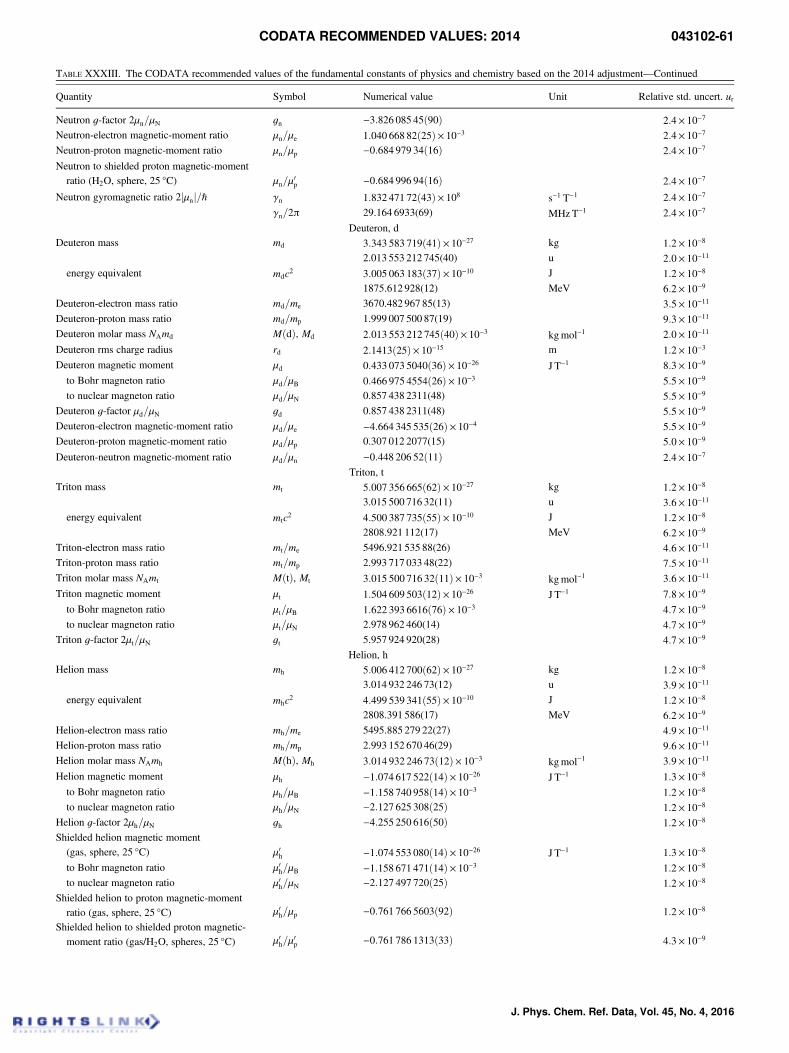
TABLE XXXIII. The CODATA recommended values of the fundamental constants of physics and chemistry based on the 2014 adjustment—Continued
Quantity Symbol Numerical value Unit Relative std. uncert. ur
Neutron g-factor 2μn=μN gn −3:826 085 45ð90Þ 2:4× 10⁻⁷
Neutron-electron magnetic-moment ratio μn=μe 1:040 668 82ð25Þ× 10−3 2:4× 10⁻⁷
Neutron-proton magnetic-moment ratio μn=μp −0:684 979 34ð16Þ 2:4× 10⁻⁷
Neutron to shielded proton magnetic-momentratio (H2O, sphere, 25 °C) μn=μ
0p −0:684 996 94ð16Þ 2:4× 10⁻⁷
Neutron gyromagnetic ratio 2jμnj=ℏ γn 1:832 471 72ð43Þ× 108 s−1 T−1 2:4× 10⁻⁷
γn=2π 29.164 6933(69) MHzT−1 2:4× 10⁻⁷
Deuteron, dDeuteron mass md 3:343 583 719ð41Þ× 10−27 kg 1:2× 10⁻⁸
2.013 553 212 745(40) u 2:0× 10−11
energy equivalent mdc2 3:005 063 183ð37Þ× 10−10 J 1:2× 10⁻⁸
1875.612 928(12) MeV 6:2× 10⁻⁹
Deuteron-electron mass ratio md=me 3670.482 967 85(13) 3:5× 10⁻¹¹
Deuteron-proton mass ratio md=mp 1.999 007 500 87(19) 9:3× 10⁻¹¹
Deuteron molar mass NAmd MðdÞ, Md 2:013 553 212 745ð40Þ× 10−3 kgmol−1 2:0× 10−11
Deuteron rms charge radius rd 2:1413ð25Þ× 10−15 m 1:2× 10⁻³
Deuteron magnetic moment μd 0:433 073 5040ð36Þ× 10−26 J T−1 8:3× 10⁻⁹
to Bohr magneton ratio μd=μB 0:466 975 4554ð26Þ× 10−3 5:5× 10⁻⁹
to nuclear magneton ratio μd=μN 0.857 438 2311(48) 5:5× 10⁻⁹
Deuteron g-factor μd=μN gd 0.857 438 2311(48) 5:5× 10⁻⁹
Deuteron-electron magnetic-moment ratio μd=μe −4:664 345 535ð26Þ× 10−4 5:5× 10⁻⁹
Deuteron-proton magnetic-moment ratio μd=μp 0.307 012 2077(15) 5:0× 10−9
Deuteron-neutron magnetic-moment ratio μd=μn −0:448 206 52ð11Þ 2:4× 10⁻⁷
Triton, tTriton mass mt 5:007 356 665ð62Þ× 10−27 kg 1:2× 10⁻⁸
3.015 500 716 32(11) u 3:6× 10⁻¹¹
energy equivalent mtc2 4:500 387 735ð55Þ× 10−10 J 1:2× 10⁻⁸
2808.921 112(17) MeV 6:2× 10⁻⁹
Triton-electron mass ratio mt=me 5496.921 535 88(26) 4:6× 10⁻¹¹
Triton-proton mass ratio mt=mp 2.993 717 033 48(22) 7:5× 10⁻¹¹
Triton molar mass NAmt MðtÞ, Mt 3:015 500 716 32ð11Þ× 10−3 kgmol−1 3:6× 10⁻¹¹
Triton magnetic moment μt 1:504 609 503ð12Þ× 10−26 J T−1 7:8× 10⁻⁹
to Bohr magneton ratio μt=μB 1:622 393 6616ð76Þ× 10−3 4:7× 10⁻⁹
to nuclear magneton ratio μt=μN 2.978 962 460(14) 4:7× 10⁻⁹
Triton g-factor 2μt=μN gt 5.957 924 920(28) 4:7× 10⁻⁹
Helion, hHelion mass mh 5:006 412 700ð62Þ× 10−27 kg 1:2× 10⁻⁸
3.014 932 246 73(12) u 3:9× 10⁻¹¹
energy equivalent mhc2 4:499 539 341ð55Þ× 10−10 J 1:2× 10⁻⁸
2808.391 586(17) MeV 6:2× 10⁻⁹
Helion-electron mass ratio mh=me 5495.885 279 22(27) 4:9× 10⁻¹¹
Helion-proton mass ratio mh=mp 2.993 152 670 46(29) 9:6× 10⁻¹¹
Helion molar mass NAmh MðhÞ, Mh 3:014 932 246 73ð12Þ× 10−3 kgmol−1 3:9× 10⁻¹¹
Helion magnetic moment μh −1:074 617 522ð14Þ× 10−26 J T−1 1:3× 10⁻⁸
to Bohr magneton ratio μh=μB −1:158 740 958ð14Þ× 10−3 1:2× 10⁻⁸
to nuclear magneton ratio μh=μN −2:127 625 308ð25Þ 1:2× 10⁻⁸
Helion g-factor 2μh=μN gh −4:255 250 616ð50Þ 1:2× 10⁻⁸
Shielded helion magnetic moment(gas, sphere, 25 °C) μ0h −1:074 553 080ð14Þ× 10−26 J T−1 1:3× 10⁻⁸
to Bohr magneton ratio μ0h=μB −1:158 671 471ð14Þ× 10−3 1:2× 10⁻⁸
to nuclear magneton ratio μ0h=μN −2:127 497 720ð25Þ 1:2× 10⁻⁸
Shielded helion to proton magnetic-momentratio (gas, sphere, 25 °C) μ0h=μp −0:761 766 5603ð92Þ 1:2× 10⁻⁸
Shielded helion to shielded proton magnetic-moment ratio (gas/H2O, spheres, 25 °C) μ0h=μ
0p −0:761 786 1313ð33Þ 4:3× 10⁻⁹
CODATA RECOMMENDED VALUES: 2014 043102-61
J. Phys. Chem. Ref. Data, Vol. 45, No. 4, 2016
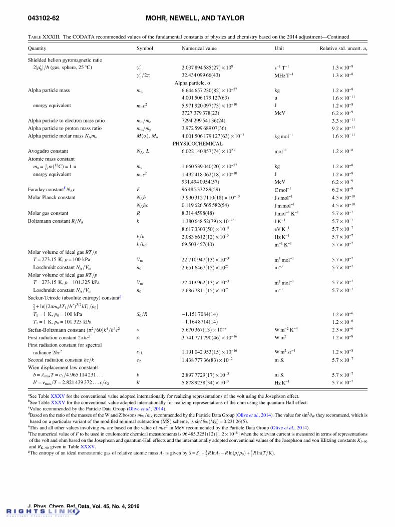
TABLE XXXIII. The CODATA recommended values of the fundamental constants of physics and chemistry based on the 2014 adjustment—Continued
Quantity Symbol Numerical value Unit Relative std. uncert. ur
Shielded helion gyromagnetic ratio2jμ0hj=ℏ (gas, sphere, 25 °C) γ0h 2:037 894 585ð27Þ× 108 s−1 T−1 1:3× 10⁻⁸
γ0h=2π 32.434 099 66(43) MHzT−1 1:3× 10⁻⁸
Alpha particle, αAlpha particle mass mα 6:644 657 230ð82Þ× 10−27 kg 1:2× 10⁻⁸
4.001 506 179 127(63) u 1:6× 10⁻¹¹
energy equivalent mαc2 5:971 920 097ð73Þ× 10−10 J 1:2× 10⁻⁸
3727.379 378(23) MeV 6:2× 10⁻⁹
Alpha particle to electron mass ratio mα=me 7294.299 541 36(24) 3:3× 10⁻¹¹
Alpha particle to proton mass ratio mα=mp 3.972 599 689 07(36) 9:2× 10⁻¹¹
Alpha particle molar mass NAmα MðαÞ, Mα 4:001 506 179 127ð63Þ× 10−3 kgmol−1 1:6× 10⁻¹¹
PHYSICOCHEMICALAvogadro constant NA, L 6:022 140 857ð74Þ× 1023 mol−1 1:2× 10⁻⁸
Atomic mass constant
mu =112mð12CÞ= 1 u mu 1:660 539 040ð20Þ× 10−27 kg 1:2× 10⁻⁸
energy equivalent muc2 1:492 418 062ð18Þ× 10−10 J 1:2× 10⁻⁸
931.494 0954(57) MeV 6:2× 10⁻⁹
Faraday constantf NAe F 96 485.332 89(59) Cmol−1 6:2× 10⁻⁹
Molar Planck constant NAh 3:990 312 7110ð18Þ× 10−10 J smol−1 4:5× 10⁻¹⁰
NAhc 0.119 626 565 582(54) Jmmol−1 4:5× 10⁻¹⁰
Molar gas constant R 8.314 4598(48) Jmol−1 K−1 5:7× 10⁻⁷
Boltzmann constant R=NA k 1:380 648 52ð79Þ× 10−23 J K−1 5:7× 10⁻⁷
8:617 3303ð50Þ× 10−5 eVK−1 5:7× 10⁻⁷
k=h 2:083 6612ð12Þ× 1010 HzK−1 5:7× 10⁻⁷
k=hc 69.503 457(40) m−1 K−1 5:7× 10⁻⁷
Molar volume of ideal gas RT=pT = 273:15 K, p= 100 kPa Vm 22:710 947ð13Þ× 10−3 m3 mol−1 5:7× 10⁻⁷
Loschmidt constant NA=Vm n0 2:651 6467ð15Þ× 1025 m−3 5:7× 10⁻⁷
Molar volume of ideal gas RT=pT = 273:15 K, p= 101:325 kPa Vm 22:413 962ð13Þ× 10−3 m3 mol−1 5:7× 10⁻⁷
Loschmidt constant NA=Vm n0 2:686 7811ð15Þ× 1025 m−3 5:7× 10⁻⁷
Sackur-Tetrode (absolute entropy) constantg
52+ ln½ð2πmukT1=h2Þ3=2kT1=p0�T1 = 1 K, p0 = 100 kPa S0=R −1:151 7084ð14Þ 1:2× 10⁻⁶
T1 = 1 K, p0 = 101:325 kPa −1:164 8714ð14Þ 1:2× 10⁻⁶
Stefan-Boltzmann constant ðπ2=60Þk4=ℏ3c2 σ 5:670 367ð13Þ× 10−8 Wm−2 K−4 2:3× 10⁻⁶
First radiation constant 2πhc2 c1 3:741 771 790ð46Þ× 10−16 Wm2 1:2× 10⁻⁸
First radiation constant for spectral
radiance 2hc2 c1L 1:191 042 953ð15Þ× 10−16 Wm2 sr−1 1:2× 10⁻⁸
Second radiation constant hc=k c2 1:438 777 36ð83Þ× 10−2 m K 5:7× 10⁻⁷
Wien displacement law constantsb= λmaxT = c2=4:965 114 231 . . . b 2:897 7729ð17Þ× 10−3 m K 5:7× 10⁻⁷
b0 = νmax=T = 2:821 439 372 . . . c=c2 b0 5:878 9238ð34Þ× 1010 HzK−1 5:7× 10⁻⁷
aSee Table XXXV for the conventional value adopted internationally for realizing representations of the volt using the Josephson effect.bSee Table XXXV for the conventional value adopted internationally for realizing representations of the ohm using the quantum-Hall effect.cValue recommended by the Particle Data Group (Olive et al., 2014).dBased on the ratio of the masses of theW and Z bosonsmW=mZ recommended by the Particle Data Group (Olive et al., 2014). The value for sin2θW they recommend, which isbased on a particular variant of the modified minimal subtraction ðMSÞ scheme, is sin2 θWðMZÞ= 0:231 26ð5Þ.eThis and all other values involving mτ are based on the value of mτc2 in MeV recommended by the Particle Data Group (Olive et al., 2014).fThe numerical value of F to be used in coulometric chemical measurements is 96 485.3251(12) [1:2× 10⁻⁸] when the relevant current is measured in terms of representationsof the volt and ohm based on the Josephson and quantum-Hall effects and the internationally adopted conventional values of the Josephson and von Klitzing constants KJ−90and RK−90 given in Table XXXV.gThe entropy of an ideal monoatomic gas of relative atomic mass Ar is given by S= S0 + 3
2R lnAr −R lnðp=p0Þ+ 52R lnðT=KÞ.
043102-62 MOHR, NEWELL, AND TAYLOR
J. Phys. Chem. Ref. Data, Vol. 45, No. 4, 2016
meeting in Paris in the fall of 2018 a resolution that will revisethe SI. In the “new SI,” as it has come to be called todistinguish it from the present SI, the definitions of thekilogram, ampere, kelvin, and mole are linked to exact valuesof the Planck constant h, elementary charge e, Boltzmannconstant k, and Avogadro constant NA, in much the same wayas the present definition of the meter is linked to an exact valueof the speed of light in vacuum c. CODATA, through its TaskGroup on Fundamental Constants, is to provide the values ofh, e, k, and NA for the new definitions by carrying out a special
least-squares adjustment during the summer of 2017. Details ofthe proposed new-SI may be found on the BIPM website atbipm.org/en/measurement-units/new-si/ [see also Milton,Davis, and Fletcher (2014)].
A. Comparison of 2014 and 2010 CODATArecommended values
Table XL compares the 2014 and 2010 recommended valuesof a representative group of constants. The regularities observed
TABLE XXXIV. The variances, covariances, and correlation coefficients of the values of a selected group ofconstants based on the 2014 CODATA adjustment. The numbers in bold above the main diagonal are 1016 times thenumerical values of the relative covariances; the numbers in bold on the main diagonal are 1016 times the numericalvalues of the relative variances; and the numbers in italics below the main diagonal are the correlation coefficients.a
α h e me NA me=mμ F
α 0:0005 0:0005 0:0005 −0:0005 0:0005 −0:0010 0:0010h 0:0176 1:5096 0:7550 1:5086 −1:5086 −0:0010 −0:7536e 0:0361 0:9998 0:3778 0:7540 −0:7540 −0:0010 −0:3763me −0:0193 0:9993 0:9985 1:5097 −1:5097 0:0011 −0:7556NA 0:0193 −0:9993 −0:9985 −1:0000 1:5097 −0:0011 0:7557me=mμ −0:0202 −0:0004 −0:0007 0:0004 −0:0004 4:9471 −0:0021F 0:0745 −0:9957 −0:9939 −0:9985 0:9985 −0:0015 0:3794
aThe relative covariance is urðxi, xjÞ= uðxi, xjÞ=ðxixjÞ, where uðxi, xjÞ is the covariance of xi and xj; the relative variance isu2r ðxiÞ= urðxi, xiÞ: and the correlation coefficient is rðxi, xjÞ= uðxi, xjÞ=½uðxiÞuðxjÞ�.
TABLE XXXV. Internationally adopted values of various quantities
Quantity Symbol Numerical value Unit Relative std. uncert. ur
Relative atomic massa of 12C Arð12CÞ 12 Exact
Molar mass constant Mu 1× 10⁻³ kg mol−1 Exact
Molar mass of 12C Mð12CÞ 12× 10−3 kg mol−1 Exact
Conventional value of Josephson constantb KJ−90 483 597.9 GHz V−1 Exact
Conventional value of von Klitzing constantc RK−90 25 812.807 Ω ExactStandard-state pressure 100 kPa ExactStandard atmosphere 101.325 kPa Exact
aThe relative atomic mass ArðXÞ of particle X with mass mðXÞ is defined by ArðXÞ=mðXÞ=mu, wheremu =mð12CÞ=12=Mu=NA = 1 u is the atomic mass constant, Mu is the molar mass constant, NA is the Avogadroconstant, and u is the unified atomic mass unit. Thus the mass of particle X is mðXÞ=ArðXÞ u and the molar mass of X isMðXÞ=ArðXÞMu.bThis is the value adopted internationally for realizing representations of the volt using the Josephson effect.cThis is the value adopted internationally for realizing representations of the ohm using the quantum-Hall effect.
TABLE XXXVI. Values of some x-ray-related quantities based on the 2014 CODATA adjustment of the values of the constants
Quantity Symbol Numerical value Unit Relative std. uncert. ur
Cu x unit: λðCuKα1Þ=1 537:400 xuðCuKα1Þ 1:002 076 97ð28Þ× 10−13 m 2:8× 10⁻⁷
Mo x unit: λðMoKα1Þ=707:831 xuðMoKα1Þ 1:002 099 52ð53Þ× 10−13 m 5:3× 10⁻⁷
Angstrom star: λðWKα1Þ=0:209 010 0 A* 1:000 014 95ð90Þ× 10−10 m 9:0× 10−7
Lattice parametera of Si (in vacuum, 22:5 °C) a 543:102 0504ð89Þ× 10−12 m 1:6× 10⁻⁸
f220g lattice spacing of Si a=ffiffiffi8
p
(in vacuum, 22:5 °C) d220 192:015 5714ð32Þ× 10−12 m 1:6× 10⁻⁸
Molar volume of Si MðSiÞ=ρðSiÞ=NAa3=8(in vacuum, 22:5 °C) VmðSiÞ 12:058 832 14ð61Þ× 10−6 m3 mol−1 5:1× 10⁻⁸
aThis is the lattice parameter (unit cell edge length) of an ideal single crystal of naturally occurring Si free of impurities and imperfections and is deduced frommeasurements onextremely pure and nearly perfect single crystals of Si by correcting for the effects of impurities.
CODATA RECOMMENDED VALUES: 2014 043102-63
J. Phys. Chem. Ref. Data, Vol. 45, No. 4, 2016
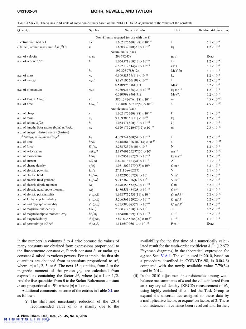
in the numbers in columns 2 to 4 arise because the values ofmany constants are obtained from expressions proportional tothe fine-structure constant α, Planck constant h, or molar gasconstant R raised to various powers. For example, the first sixquantities are obtained from expressions proportional to αa,where jaj= 1, 2, 3, or 6. The next 15 quantities, from h to themagnetic moment of the proton μp, are calculated fromexpressions containing the factor ha, where jaj= 1 or 1=2.And the five quantities from R to the Stefan-Boltzmann constantσ are proportional to Ra, where jaj= 1 or 4.
Additional comments on some of the entries in Table XL areas follows.
(i) The shift and uncertainty reduction of the 2014recommended value of α is mainly due to the
availability for the first time of a numerically calcu-lated result for the tenth-order coefficient Að10Þ
1 (12 672Feynman diagrams) in the theoretical expression forae; see Sec. V.A.1. The value used in 2010, based ona procedure described in CODATA-98, is 0.0(4.6)compared with the newly available value 7.79(34)used in 2014.
(ii) In the 2010 adjustment inconsistencies among watt-balance measurements of h and the value inferred froman x-ray-crystal-density (XRCD) measurement of NA
using highly enriched silicon led the Task Group toexpand the uncertainties assigned to these data bya multiplicative factor, or expansion factor, of 2. Theseinconsistencies have since been resolved and further,
TABLE XXXVII. The values in SI units of some non-SI units based on the 2014 CODATA adjustment of the values of the constants
Quantity Symbol Numerical value Unit Relative std. uncert. ur
Non-SI units accepted for use with the SIElectron volt: (e=C) J eV 1:602 176 6208ð98Þ× 10−19 J 6:1× 10⁻⁹
(Unified) atomic mass unit: 112mð12CÞ u 1:660 539 040ð20Þ× 10−27 kg 1:2× 10⁻⁸
Natural units (n.u.)n.u. of velocity c, c0 299 792 458 m s−1 Exact
n.u. of action: h=2π ℏ 1:054 571 800ð13Þ× 10−34 J s 1:2× 10⁻⁸
6:582 119 514ð40Þ× 10−16 eV s 6:1× 10⁻⁹
ℏc 197.326 9788(12) MeV fm 6:1× 10⁻⁹
n.u. of mass me 9:109 383 56ð11Þ× 10−31 kg 1:2× 10⁻⁸
n.u. of energy mec2 8:187 105 65ð10Þ× 10−14 J 1:2× 10⁻⁸
0.510 998 9461(31) MeV 6:2× 10⁻⁹
n.u. of momentum mec 2:730 924 488ð34Þ× 10−22 kgm s−1 1:2× 10⁻⁸
0.510 998 9461(31) MeV/c 6:2× 10⁻⁹
n.u. of length: ℏ=mec ƛC 386:159 267 64ð18Þ× 10−15 m 4:5× 10⁻¹⁰
n.u. of time ℏ=mec2 1:288 088 667 12ð58Þ× 10−21 s 4:5× 10⁻¹⁰
Atomic units (a.u.)a.u. of charge e 1:602 176 6208ð98Þ× 10−19 C 6:1× 10⁻⁹
a.u. of mass me 9:109 383 56ð11Þ× 10−31 kg 1:2× 10⁻⁸
a.u. of action: h=2π ℏ 1:054 571 800ð13Þ× 10−34 J s 1:2× 10⁻⁸
a.u. of length: Bohr radius (bohr) α=4πR∞ a0 0:529 177 210 67ð12Þ× 10−10 m 2:3× 10⁻¹⁰
a.u. of energy: Hartree energy (hartree)
e2=4πe0a0 = 2R∞hc=α2mec2 Eh 4:359 744 650ð54Þ× 10−18 J 1:2× 10⁻⁸
a.u. of time ℏ=Eh 2:418 884 326 509ð14Þ× 10−17 s 5:9× 10⁻¹²
a.u. of force Eh=a0 8:238 723 36ð10Þ× 10−8 N 1:2× 10⁻⁸
a.u. of velocity: αc a0Eh=ℏ 2:187 691 262 77ð50Þ× 106 m s−1 2:3× 10⁻¹⁰
a.u. of momentum ℏ=a0 1:992 851 882ð24Þ× 10−24 kgm s−1 1:2× 10⁻⁸
a.u. of current eEh=ℏ 6:623 618 183ð41Þ× 10−3 A 6:1× 10⁻⁹
a.u. of charge density e=a30 1:081 202 3770ð67Þ× 1012 C m−3 6:2× 10⁻⁹
a.u. of electric potential Eh=e 27.211 386 02(17) V 6:1× 10⁻⁹
a.u. of electric field Eh=ea0 5:142 206 707ð32Þ× 1011 V m−1 6:1× 10⁻⁹
a.u. of electric field gradient Eh=ea20 9:717 362 356ð60Þ× 1021 V m−2 6:2× 10⁻⁹
a.u. of electric dipole moment ea0 8:478 353 552ð52Þ× 10−30 C m 6:2× 10⁻⁹
a.u. of electric quadrupole moment ea20 4:486 551 484ð28Þ× 10−40 Cm2 6:2× 10⁻⁹
a.u. of electric polarizability e2a20=Eh 1:648 777 2731ð11Þ× 10−41 C2 m2 J−1 6:8× 10⁻¹⁰
a.u. of 1st hyperpolarizability e3a30=E2h 3:206 361 329ð20Þ× 10−53 C3 m3 J−2 6:2× 10⁻⁹
a.u. of 2nd hyperpolarizability e4a40=E3h 6:235 380 085ð77Þ× 10−65 C4 m4 J−3 1:2× 10⁻⁸
a.u. of magnetic flux density ℏ=ea20 2:350 517 550ð14Þ× 105 T 6:2× 10⁻⁹
a.u. of magnetic dipole moment: 2μB ℏe=me 1:854 801 999ð11Þ× 10−23 J T−1 6:2× 10⁻⁹
a.u. of magnetizability e2a20=me 7:891 036 5886ð90Þ× 10−29 J T−2 1:1× 10⁻⁹
a.u. of permittivity: 107=c2 e2=a0Eh 1:112 650 056 . . . × 10−10 Fm−1 Exact
043102-64 MOHR, NEWELL, AND TAYLOR
J. Phys. Chem. Ref. Data, Vol. 45, No. 4, 2016
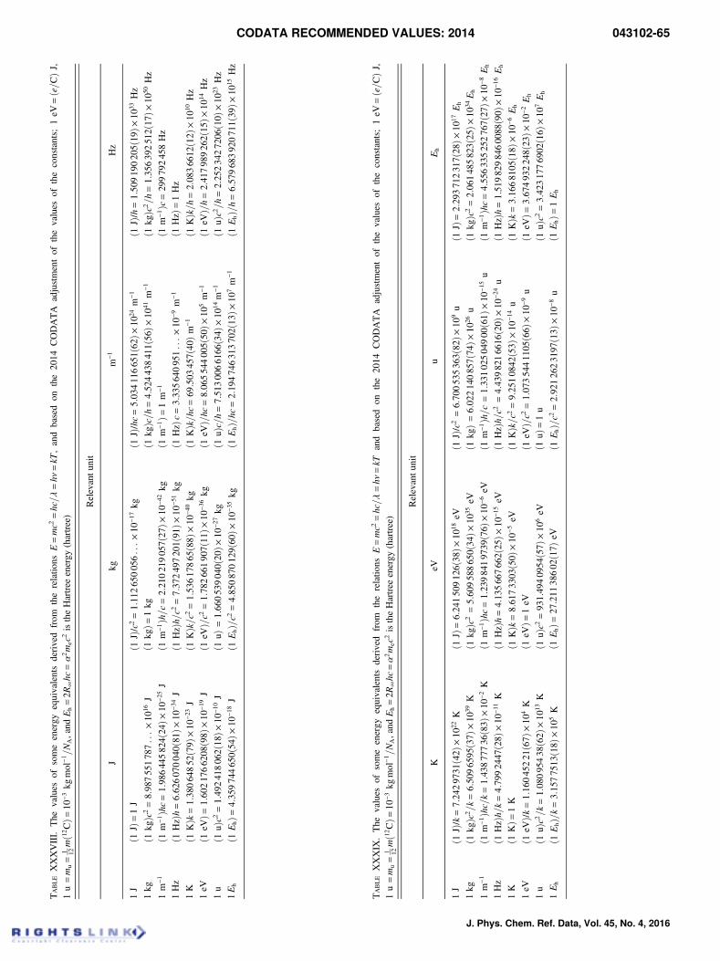
TABLEXXXVIII.
The
values
ofsomeenergy
equivalentsderivedfrom
therelatio
nsE=mc2
=hc=λ=hν
=kT
,andbasedon
the20
14CODATA
adjustmentof
thevalues
oftheconstants;
1eV
=ðe=
CÞJ
,1u=m
u=
1 12mð12
CÞ=
10−3
kgmol
−1=NA,and
Eh=2R
∞hc
=α2m
ec2istheHartree
energy
(hartree)
Relevantu
nit
Jkg
m−1
Hz
1J
ð1JÞ=1J
ð1JÞ/
c2=1:11
265
005
6...×10
−17kg
ð1JÞ/
hc=5:03
411
665
1ð62Þ×
1024
m−1
ð1JÞ/
h=1:50
919
020
5ð19
Þ×10
33Hz
1kg
ð1kgÞc2
=8:98
755
178
7...×10
16J
ð1kgÞ=
1kg
ð1kgÞc=
h=4:52
443
841
1ð56Þ×
1041
m−1
ð1kgÞc2
=h=1:35
639
251
2ð17Þ×
1050
Hz
1m
−1ð1
m−1Þhc=1:98
644
582
4ð24Þ×
10−2
5J
ð1m
−1Þh=c=2:21
021
905
7ð27Þ×
10−4
2kg
ð1m
−1Þ=
1m
−1ð1
m−1Þc=29
979
245
8Hz
1Hz
ð1HzÞh
=6:62
607
004
0ð81Þ×
10−3
4J
ð1HzÞh
=c2
=7:37
249
720
1ð91Þ×
10−5
1kg
ð1HzÞc=3:33
564
095
1...×10
−9m
−1ð1
HzÞ=1Hz
1K
ð1KÞk
=1:38
064
852ð79Þ
×10
−23J
ð1KÞk=
c2=1:53
617
865ð88Þ
×10
−40kg
ð1KÞk=
hc=69:503
457ð40Þm
−1ð1
KÞk=
h=2:08
366
12ð12Þ
×10
10Hz
1eV
ð1eV
Þ=1:60
217
662
08ð98Þ
×10
−19J
ð1eV
Þ=c2
=1:78
266
190
7ð11Þ×
10−3
6kg
ð1eV
Þ=hc
=8:06
554
400
5ð50Þ×
105m
−1ð1
eVÞ=h=2:41
798
926
2ð15Þ×
1014
Hz
1u
ð1uÞc2=1:49
241
806
2ð18Þ×
10−1
0J
ð1uÞ
=1:66
053
904
0ð20
Þ×10
−27kg
ð1uÞc=h=7:51
300
661
66ð34Þ
×10
14m
−1ð1
uÞc2=h=2:25
234
272
06ð10Þ
×10
23Hz
1Eh
ð1EhÞ=
4:35
974
465
0ð54Þ×
10−1
8J
ð1EhÞ=c2=4:85
087
012
9ð60
Þ×10
−35kg
ð1EhÞ=hc
=2:19
474
631
370
2ð13Þ×
107m
−1ð1
EhÞ=h=6:57
968
392
071
1ð39Þ×
1015
Hz
TABLEXXXIX
.The
values
ofsomeenergy
equivalentsderived
from
therelatio
nsE=mc2=hc=λ=hν
=kT
and
based
onthe20
14CODATA
adjustmentof
thevalues
oftheconstants;
1eV
=ðe=
CÞJ
,1u=m
u=
1 12mð12
CÞ=
10−3
kgmol
−1=NA,and
Eh=2R
∞hc
=α2m
ec2istheHartree
energy
(hartree)
Relevantu
nit
KeV
uEh
1J
ð1JÞ/
k=7:24
297
31ð42Þ
×10
22K
ð1JÞ=6:24
150
912
6ð38Þ×
1018
eVð1
JÞ/c2
=6:70
053
536
3ð82Þ×
109u
ð1JÞ=2:29
371
231
7ð28Þ×
1017
Eh
1kg
ð1kgÞc2
=k=6:50
965
95ð37Þ
×10
39K
ð1kgÞc2
=5:60
958
865
0ð34Þ×
1035
eVð1
kgÞ=
6:02
214
085
7ð74Þ×
1026
uð1
kgÞc2
=2:06
148
582
3ð25Þ×
1034Eh
1m
−1ð1
m−1Þhc=k=1:43
877
736ð83Þ
×10
−2K
ð1m
−1Þhc=1:23
984
197
39ð76Þ
×10
−6eV
ð1m
−1Þh=c=1:33
102
504
900ð61Þ
×10
−15u
ð1m
−1Þhc=4:55
633
525
276
7ð27Þ×
10−8
Eh
1Hz
ð1HzÞh
=k=4:79
924
47ð28Þ
×10
−11K
ð1HzÞh
=4:13
566
766
2ð25Þ×
10−1
5eV
ð1HzÞh
=c2
=4:43
982
166
16ð20Þ
×10
−24u
ð1HzÞh
=1:51
982
984
600
88ð90Þ
×10
−16Eh
1K
ð1KÞ=
1K
ð1KÞk
=8:61
733
03ð50Þ
×10
−5eV
ð1KÞk=
c2=9:25
108
42ð53Þ
×10
−14u
ð1KÞk
=3:16
681
05ð18Þ
×10
−6Eh
1eV
ð1eV
Þ/k=1:16
045
221ð67Þ
×10
4K
ð1eV
Þ=1eV
ð1eV
Þ=c2=1:07
354
411
05ð66Þ
×10
−9u
ð1eV
Þ=3:67
493
224
8ð23Þ×
10−2
Eh
1u
ð1uÞc2=k=1:08
095
438ð62Þ
×10
13K
ð1uÞc2
=93
1:49
409
54ð57Þ
×10
6eV
ð1uÞ
=1u
ð1uÞc2=3:42
317
769
02ð16Þ
×10
7Eh
1Eh
ð1EhÞ=k=3:15
775
13ð18Þ
×10
5K
ð1EhÞ=
27:211
38602ð17Þ
eVð1
EhÞ=c2
=2:92
126
231
97ð13Þ
×10
−8u
ð1EhÞ=
1Eh
CODATA RECOMMENDED VALUES: 2014 043102-65
J. Phys. Chem. Ref. Data, Vol. 45, No. 4, 2016
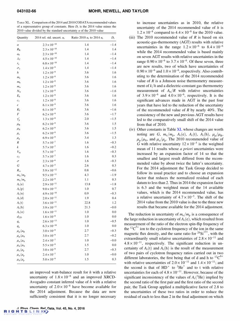
an improved watt-balance result for h with a relativeuncertainty of 1:8× 10⁻⁸ and an improved XRCD-Avogadro constant inferred value of h with a relativeuncertainty of 2:0× 10−8 have become available forthe 2014 adjustment. Because the data are nowsufficiently consistent that it is no longer necessary
to increase uncertainties as in 2010, the relativeuncertainty of the 2014 recommended value of h is1:2× 10⁻⁸ compared to 4:4× 10⁻⁸ for the 2010 value.
(iii) The 2010 recommended value of R is based on sixacoustic-gas-thermometry (AGT) results with relativeuncertainties in the range 1:2× 10⁻⁶ to 8:4× 10⁻⁶
while the 2014 recommended value is based mainlyon seven AGT results with relative uncertainties in therange 0:90× 10−6 to 3:7× 10⁻⁶. Of these seven, threeare new results, two of which have uncertainties of0:90× 10−6 and 1:0× 10−6, respectively. Also contrib-uting to the determination of the 2014 recommendedvalue of R is a Johnson noise thermometry measure-ment of k=h and a dielectric-constant gas thermometrymeasurement of Ae=R with relative uncertaintiesof 3:9× 10⁻⁶ and 4:0× 10−6, respectively. It is thesignificant advances made in AGT in the past fouryears that have led to the reduction of the uncertaintyof the recommended value of R by nearly 40%. Theconsistency of the new and previous AGT results haveled to the comparatively small shift of the 2014 valuefrom that of 2010.
(iv) Other constants in Table XL whose changes are worthnoting are G, me=mp, ArðeÞ, ArðtÞ, ArðhÞ, μp=μB,μp=μN, and μe=μp. The 2010 recommended value ofG with relative uncertainty 12× 10−5 is the weightedmean of 11 results whose a priori uncertainties wereincreased by an expansion factor of 14 so that thesmallest and largest result differed from the recom-mended value by about twice the latter’s uncertainty.For the 2014 adjustment the Task Group decided tofollow its usual practice and to choose an expansionfactor that reduces the normalized residual of eachdatum to less than 2. Thus in 2014 the expansion factoris 6.3 and the weighted mean of the 14 availablevalues, which is the 2014 recommended value, hasa relative uncertainty of 4:7× 10⁻⁵. The shift of the2014 value from the 2010 value is due to the three newresults that became available for the 2014 adjustment.
The reduction in uncertainty of me=mp is a consequence ofthe large reduction in uncertainty of ArðeÞ, which resulted frommeasurement of the ratio of the electron spin-flip frequency ofthe 12C5+ ion to the cyclotron frequency of the ion in the samemagnetic flux density, and the same ratio for 28Si13+, with theextraordinarily small relative uncertainties of 2:8× 10⁻¹¹ and4:8× 10⁻¹¹, respectively. The significant reduction in un-certainty of ArðtÞ and ArðhÞ is the result of the measurementof two pairs of cyclotron frequency ratios carried out in twodifferent laboratories, the first being that of d and h to 12C6+
with relative uncertainties of 2:0× 10−11 and 1:4× 10⁻¹¹; andthe second is that of HD+ to 3He+ and to t with relativeuncertainties for each of 4:8× 10⁻¹¹. However, because of thesignificant inconsistency of the values of Arð3HeÞ implied bythe second ratio of the first pair and the first ratio of the secondpair, the Task Group applied a multiplicative factor of 2.8 tothe uncertainties of these two ratios in order to reduce theresidual of each to less than 2 in the final adjustment on which
TABLE XL. Comparison of the 2014 and 2010 CODATA recommended valuesof a representative group of constants. Here Dr is the 2014 value minus the2010 value divided by the standard uncertainty u of the 2010 value
Quantity 2014 rel. std. uncert. ur Ratio 2010 ur to 2014 ur Dr
α 2:3× 10⁻¹⁰ 1.4 −1:4RK 2:3× 10⁻¹⁰ 1.4 1.4
a0 2:3× 10⁻¹⁰ 1.4 −1:4λC 4:5× 10⁻¹⁰ 1.4 −1:4re 6:8× 10⁻¹⁰ 1.4 −1:4σe 1:4× 10⁻⁹ 1.4 −1:4h 1:2× 10⁻⁸ 3.6 1.6
me 1:2× 10⁻⁸ 3.6 1.6
mh 1:2× 10⁻⁸ 3.6 1.6
mα 1:2× 10⁻⁸ 3.6 1.6
NA 1:2× 10⁻⁸ 3.6 −1:6Eh 1:2× 10⁻⁸ 3.6 1.6
c1 1:2× 10⁻⁸ 3.6 1.6
e 6:1× 10⁻⁹ 3.6 1.6
KJ 6:1× 10⁻⁹ 3.6 −1:6F 6:2× 10⁻⁹ 3.6 −1:7γ0p 1:3× 10⁻⁸ 2.0 −1:5μB 6:2× 10⁻⁹ 3.6 1.5
μN 6:2× 10⁻⁹ 3.6 1.5
μe 6:2× 10⁻⁹ 3.6 −1:5μp 6:9× 10⁻⁹ 3.4 1.3
R 5:7× 10⁻⁷ 1.6 −0:3k 5:7× 10⁻⁷ 1.6 −0:2Vm 5:7× 10⁻⁷ 1.6 −0:3c2 5:7× 10⁻⁷ 1.6 0.3
σ 2:3× 10⁻⁶ 1.6 −0:3G 4:7× 10⁻⁵ 2.6 0.3
R∞ 5:9× 10⁻¹² 0.8 −0:6me=mp 9:5× 10⁻¹¹ 4.3 −1:9me=mμ 2:2× 10⁻⁸ 1.1 0.3
ArðeÞ 2:9× 10⁻¹¹ 13.8 −1:8ArðpÞ 9:0× 10−11 1.0 0.7
ArðnÞ 4:9× 10⁻¹⁰ 0.9 −0:3ArðdÞ 2:0× 10−11 1.9 0.4
ArðtÞ 3:6× 10⁻¹¹ 22.8 1.2
ArðhÞ 3:9× 10⁻¹¹ 21.3 −0:0ArðαÞ 1:6× 10⁻¹¹ 1.0 0.0
d220 1:6× 10⁻⁸ 1.0 0.0
ge 2:6× 10⁻¹³ 1.0 −0:5gμ 6:3× 10⁻¹⁰ 1.0 0.0
μp=μB 3:0× 10−9 2.7 −0:3μp=μN 3:0× 10−9 2.7 −0:2μn=μN 2:4× 10⁻⁷ 1.0 −0:0μd=μN 5:5× 10⁻⁹ 1.5 0.0
μe=μp 3:0× 10−9 2.7 −0:3μn=μp 2:4× 10⁻⁷ 1.0 −0:0μd=μp 5:0× 10−9 1.5 0.3
043102-66 MOHR, NEWELL, AND TAYLOR
J. Phys. Chem. Ref. Data, Vol. 45, No. 4, 2016
the 2014 recommended values are based. Finally, the reductionin the uncertainties of μp=μB, μp=μN, and μe=μp are a conse-quence of a new, directly measured value of μp=μN witha relative uncertainty of 3:3× 10⁻⁹.
B. Some implications of the 2014 CODATArecommended values and adjustment
for metrology and physics
1. Conventional electrical units
The conventional values KJ−90 = 483 597:9 GHz=V andRK−90 = 25 812:807 Ω adopted in 1990 for the Josephson andvon Klitzing constants established conventional units of voltageand resistance, V90 and Ω90, given by V90 = ðKJ−90=KJÞ V andΩ90 = ðRK=RK−90Þ Ω. Other conventional electric units followfrom V90 and Ω90, for example, A90 =V90=Ω90, C90 =A90 s,W90 =A90V90, F90 =C90=V90, and H90 =Ω90 s, which are theconventional units of current, charge, power, capacitance, andinductance, respectively, (Taylor and Mohr, 2001). The 2014adjustment gives for the relations between KJ and KJ−90, and forRK and RK−90,
KJ =KJ−90½1− 9:83ð61Þ× 10−8� , (273)
RK =RK−90½1+ 1:765ð23Þ× 10−8� , (274)
which lead to
V90 = ½1+ 9:83ð61Þ× 10−8� V, (275)
Ω90 = ½1+ 1:765ð23Þ× 10−8� Ω , (276)
A90 = ½1+ 8:06ð61Þ× 10−8� A, (277)
C90 = ½1+ 8:06ð61Þ× 10−8� C, (278)
W90 = ½1+ 17:9ð1:2Þ× 10−8� W, (279)
F90 = ½1− 1:765ð23Þ× 10−8� F, (280)
H90 = ½1+ 1:765ð23Þ× 10−8� H. (281)
Equations (275) and (276) show that V90 exceeds V and Ω90
exceeds Ω, which means that measured voltages and re-sistances traceable to the Josephson effect and KJ−90 and thequantum-Hall effect and RK−90, respectively, are too smallrelative to the SI. However, the differences are well within the40× 10−8 uncertainty assigned to V90= V and the 10× 10−8
uncertainty assigned to Ω90=Ω by the Consultative Committeefor Electricity and Magnetism (CCEM) of the InternationalCommittee for Weights and Measures (CIPM) (Quinn, 1989;Quinn, 2001).
2. Josephson and quantum-Hall effects
Watt-balance and XRCD-NA advances have led to testsof the exactness of the quantum-Hall and Josephson effectrelations RK = h=e2 and KJ = 2e=h that are less clouded byinconsistencies of the data. Indeed, based on the 2014 data as usedin adjustment 2 summarized in Table XXVIII, Sec. XIII.B.2, thepossible corrections eK and eJ to the quantum-Hall and Josephsoneffect relations are 2:2ð1:8Þ× 10−8 and −0:9ð1:5Þ× 10−8, re-spectively; see Table XXXI, Sec. XIII.B.3. Thus the exactness
of these relations is experimentally confirmed within about 2parts in 108. However, as Table XXXI indicates, some of theinitial 2014 input data are not as supportive of the exactness ofthe relations, most notably the NIST-89 result for Γ0
p−90; on theother hand, its normalized residual in the adjustment thatproduced the above values of eK and eJ is 2.3 and because ofits low-weight it is omitted from the 2006 and 2010 finaladjustments as well as the 2014 final adjustment.
3. The new SI
The impact of the new data that have become available forthe 2014 adjustment on the establishment of the new SI by theCGPM is discussed in detail in the Introduction section of thisreport (see Sec. I.B.1) and need not be repeated here. Suffice itto say that the uncertainties of the 2014 recommended valuesof the four new defining constants h, e, k, and NA, which inparts in 108 are 1.2, 0.61, 57, and 1.2, are already sufficientlysmall to meet the requirements deemed necessary by the CIPMand CGPM for the adoption of the new SI.
4. Proton radius
The severe disagreement of the proton rms charge radius rpdetermined from the Lamb shift in muonic hydrogen withvalues determined from H and D transition frequencies andelectron-proton scattering experiments present in the 2010adjustment remain present in the 2014 adjustment. Althoughthe uncertainty of the muonic hydrogen value is significantlysmaller than the uncertainties of these other values, its negativeimpact on the internal consistency of the theoretically pre-dicted and experimentally measured frequencies, as well as onthe value of the Rydberg constant, was considered by the TaskGroup to be still so severe that the only recourse was to onceagain exclude it from the final adjustment.
5. Muon magnetic-moment anomaly
The long-standing significant difference between the theo-retically predicted, standard-model value of aμ and theexperimentally determined value that led to the exclusion ofthe theoretical expression for aμ from the 2010 adjustmentremains; the difference is still at about the 3σ level dependingon the way the all-important lowest-order hadronic vacuumpolarization and hadronic light-by-light contributions areevaluated. Because of the continuing difficulty of reliablycalculating these terms, the Task Group decided to omit thetheory from the 2014 adjustment as in 2010. The 2014recommended values of aμ and those of other constants thatdepend on it are, therefore, based on experiment.
6. Electron magnetic-moment anomaly,fine-structure constant, and QED
A useful test of the QED theory of ae is to compare twovalues of α: The first, with relative uncertainty 2:4× 10⁻¹⁰, isthat obtained by equating the experimental value of ae with itsQED theoretical expression; the second, which is only weakly
CODATA RECOMMENDED VALUES: 2014 043102-67
J. Phys. Chem. Ref. Data, Vol. 45, No. 4, 2016
dependent on QED theory and with relative uncertainty6:2× 10⁻¹⁰, is that obtained from the measurement ofh=mð87RbÞ using atom interferometry. These two values (seethe first and second rows in Table XX, Sec. XIII.A) differ by1.8 times the uncertainty of their difference, or 1:8σ. Althoughthis is acceptable agreement and supports the QED theory ofae, the result of the same comparison in CODATA-10 based onthe same experimental values of ae and h=mð87RbÞ is 0:4σ.The two main reasons for this rather significant change are thenew and somewhat surprisingly large value of the Að10Þ
1
coefficient in the theoretical expression for ae which decreasedthe ae value of α; and the decreased but highly accurate newvalue of ArðeÞ which increased the h=mð87RbÞ value of α.
C. Suggestions for future work
As discussed, to deal with data inconsistencies the TaskGroup decided to (i) omit from the 2014 adjustment the valueof rp obtained from measurements of the Lamb shift in muonichydrogen; (ii) omit the theory of the muon magnetic-momentanomaly aμ; (iii) increase the initial uncertainties of thecyclotron frequency ratios ωcðhÞ=ωcð12C6+Þ andωcðHD+Þ/ωcð3He+Þ relevant to the determination of ArðhÞ byan expansion factor of 2.8; and (iv) increase the initialuncertainties of the 14 values of G by an expansion factor of6.3. Issues (i), (ii), and (iv) have been with us for some time andsuggestions for their resolution were given in CODATA-10.Updated versions follow together with a suggestion regard-ing (iii).
As also discussed, the data now available provide values ofthe defining constants h, e, k, and NA of the new SI withuncertainties sufficiently small for its adoption by the 26thCGPM in the fall of 2018 as planned. The final values are to bebased on a special adjustment carried out by the Task Groupduring the summer of 2017. Because of its importance, theCIPM has decided that all the data to be used in that adjustmentmust have been published in an archival journal or be availablein a preprint accepted for publication by 1 July 2017.Nevertheless, we include suggestions for work that willimprove the robustness of the currently available data thatdetermine these important constants.
(i) Work currently underway could solve the “protonradius puzzle” and should continue to be pursued asvigorously as possible. This includes the measurementof hydrogen transition frequencies, the analysis of μ-pand μ-d data, and possible new Lamb-shift measure-ments in μ-h and μ-α. New scattering data fromexperiments such as MUSE (Downie, 2014) and PRad(Gasparian, 2014) and improved methods to extract rpfrom such data as well as verification of the theory ofH, D, and muonic hydrogenlike energy levels couldalso help.
(ii) Because the disagreement between aμ theory andexperiment remains even after many years of effortdevoted to improving the theory and the experimentalresults on which the theory relies, the solution to theproblem may have to wait until the completion over
the next 5 to 10 years of the two new experimentsunderway to remeasure aμ (Mibe, 2011; Logashenkoet al., 2015). Improved measurements of cross sectionsfor the scattering of e+ e− into hadrons and better dataon the decay of the τ into hadrons could also be useful.
(iii) The two cyclotron frequency ratios in question wereobtained from experiments at the University ofWashington and at Florida State University (FSU). Acareful study of the University of Washington appa-ratus that might uncover an overlooked systematiceffect is not possible because it is no longer available.However, the research program at FSU continues andthe researchers are encouraged to search for a possibleexplanation of the disagreement. An experiment underway to measure the Q value of tritium at the Max-Planck Institut fur Kernphysik, Heidelberg, Germany,could resolve the problem (Streubel et al., 2014).
(iv) One or more measurements ofGwith an uncertainty of1 part in 105 using new and innovative approachesmight finally resolve some of the problems that haveplagued the reliable determination of G over the pastthree decades. The possibliity of transferring theapparatus used by Quinn et al. (2014) and by Parksand Faller (2014) to other laboratories to be used thereby new researchers in the hope of uncovering over-looked systematic effects could be helpful as well.
(v) Watt-balance and watt-balance-like measurements ofh and the XRCD measurement of NA currently underway should continue to be vigorously pursued with thegoal of achieving uncertainties of no more than a fewparts in 108. This also applies to experiments todetermine R, k=h, and Ae=R with an uncertainty goalof no more than a few parts in 106. An independentcalculation of the Að8Þ
1 and Að10Þ1 coefficients in the
theoretical expression for ae would increase confi-dence in the value of α from ae. For this same reason,results from experiments currently under way todetermine h=mðXÞ with an uncertainty small enoughto provide a value of αwith an uncertainty of 5 parts in1010 or less would be valuable.
List of Symbols and Abbreviations
ASD NIST Atomic Spectra Database (online)AMDC AtomicMass Data Center, transferred in 2013 to
Institute of Modern Physics (IMP), ChineseAcademy of Sciences, Lanzhou, PRC, fromCentre de Spectrometrie Nucleaire et de Spec-trometrie de Masse (CSNSM), Orsay, France
AME Atomic mass evaluation from the AMDC(completed in year specified)
ArðXÞ relative atomic mass of X: ArðXÞ=mðXÞ=mu
A90 conventional unit of electric current:A90 =V90=Ω90
A*
angstrom star: λðWKα1Þ= 0:209 010 0 A*
043102-68 MOHR, NEWELL, AND TAYLOR
J. Phys. Chem. Ref. Data, Vol. 45, No. 4, 2016
ae electron magnetic-moment anomaly:ae = ðjgej− 2Þ/2
aμ muon magnetic-moment anomaly:aμ = ðjgμj− 2Þ/2
BIPM International Bureau of Weights and Measures,Sevres, France
BNL Brookhaven National Laboratory, Upton,New York, USA
CERN European Organization for Nuclear Research,Geneva, Switzerland
CGPM General Conference on Weights and MeasuresCIPM International Committee for Weights and
MeasuresCODATA Committee on Data for Science and Technology
of the International Council for ScienceCPT combined charge conjugation, parity inversion,
and time reversalc speed of light in vacuumd deuteron (nucleus of deuterium D, or 2H)d220 f220g lattice spacing of an ideal crystal of
naturally occurring silicond220ðXÞ f220g lattice spacing of crystal X of naturally
occurring silicone symbol for either member of the electron-
positron pair; when necessary, e− or e+ is used toindicate the electron or positron
e elementary charge: absolute value of the chargeof the electron
F Faraday constant: F =NAeFSU Florida State University, Tallahassee, Florida,
USAFSUJ Friedrich-Schiller University, Jena, GermanyF 90 F 90 = ðF=A90ÞAG Newtonian constant of gravitationg local acceleration due to gravitygd deuteron g-factor: gd = μd=μNge electron g-factor: ge = 2μe=μBgp proton g-factor: gp = 2μp=μNg0p shielded proton g-factor: g0p = 2μ0p=μNgt triton g-factor: gt = 2μt=μNgXðYÞ g-factor of particle X in the ground (1S) state of
hydrogenic atom Ygμ muon g-factor: gμ = 2μμ=ðeℏ=2mμÞGSI Gesellschaft fur Schweironenforschung,
Darmstadt, GermanyHD HD molecule (bound state of hydrogen and
deuterium atoms)HT HT molecule (bound state of hydrogen and
tritium atoms)HUST Huazhong University of Science and Technol-
ogy, Wuhan, PRCh helion (nucleus of 3He)h Planck constantℏ reduced Planck constant; h=2πHarvU Harvard University, Cambridge, Massachusetts,
USAIAC International Avogadro Coordination
ILL Institut Max von Laue-Paul Langevin,Grenoble, France
INRIM Istituto Nazionale di Ricerca Metrologica,Torino, Italy
IRMM Institute for Reference Materials and Measure-ments, Geel, Belgium
JILA JILA, University of Colorado and NIST,Boulder, Colorado, USA
KRISS Korea Research Institute of Standards and Sci-ence, Taedok Science Town, Republic of Korea
KR/VN KRISS-VNIIM collaborationKJ Josephson constant: KJ = 2e=hKJ−90 conventional value of the Josephson constant
KJ: KJ−90 = 483 597:9 GHzV−1
k Boltzmann constant: k =R=NA
LAMPF Clinton P. Anderson Meson Physics Facility atLos Alamos National Laboratory, Los Alamos,New Mexico, USA
LANL Los Alamos National Laboratory, Los Alamos,New Mexico, USA
LENS European Laboratory for Non-Linear Spectros-copy, University of Florence, Italy
LKB Laboratoire Kastler-Brossel, Paris, FranceLK/SY LKB and SYRTE collaborationLNE Laboratoire national de metrologie et d’essais,
Trappes, FranceMIT Massachusetts Institute of Technology,
Cambridge, Massachusetts, USAMETAS Federal Institute for Metrology, Bern-Wabern,
SwitzerlandMPIK Max-Planck-Institut fur Kernphysik,
Heidelberg, GermanyMPQ Max-Planck-Institut fur Quantenoptik,
Garching, GermanyMSL Measurement Standards Laboratory, Lower
Hutt, New ZelandMðXÞ molar mass of X: MðXÞ=ArðXÞMu
Mu muonium (μ+e− atom)Mu molar mass constant: Mu = 10−3 kg mol−1
mu unified atomic mass constant: mu =mð12CÞ/12mX , mðXÞ mass of X (for the electron e, proton p, and other
elementary particles, the first symbol is used,i.e., me, mp, etc.)
NA Avogadro constantNIM National Institute of Metrology, Beijing, PRCNIST National Institute of Standards and Technology,
Gaithersburg, Maryland and Boulder, Colorado,USA
NMI National Metrology Institute, Lindfield,Australia
NMIJ National Metrology Institute of Japan, Tsukuba,Japan
NPL National Physical Laboratory, Teddington, UKNRC National Research Council of Canada, Mea-
surement Science and Standards, Ottawa, Ontario,Canada
n neutron
CODATA RECOMMENDED VALUES: 2014 043102-69
J. Phys. Chem. Ref. Data, Vol. 45, No. 4, 2016
PTB Physikalisch-Technische Bundesanstalt,Braunschweig and Berlin, Germany
p protonQED quantum electrodynamicspðχ2jνÞ probability that an observed value of chi-square
for ν degrees of freedom would exceed χ2
R molar gas constantR ratio of muon anomaly difference frequency to
free proton NMR frequencyRB Birge ratio: RB = ðχ2=νÞ12rd bound-state rms charge radius of the deuteronRK von Klitzing constant: RK = h=e2
RK−90 conventional value of the von Klitzing constantRK: RK−90 = 25 812:807 Ω
rp bound-state rms charge radius of the protonR∞ Rydberg constant: R∞ =mecα2=2hrðxi, xjÞ correlation coefficient of estimated values xi and
xj: rðxi, xjÞ= uðxi, xjÞ=½uðxiÞuðxjÞ�Sc self-sensitivity coefficientSI Systeme international d’unites (International
System of Units)StPtrsb various institutions in St. Petersburg, Russian
FederationStanfU Stanford University, Stanford, California, USASUREC Scottish Universities Environmental Research
Centre, University of Glasgow, Glasgow, ScotlandSYRTE Systemes de reference Temps Espace, Paris,
FranceT thermodynamic temperatureTR&D Tribotech Research and Development Com-
pany, Moscow, Russian FederationType A uncertainty evaluation by the statistical analysis
of series of observationsType B uncertainty evaluation by means other than the
statistical analysis of series of observationst triton (nucleus of tritium T, or 3H)UCI University of California, Irvine, Irvine, California,
USAUMZ Institut fur Physik, Johannes Gutenberg
Universitat Mainz (or simply the University ofMainz), Mainz, Germany
USussex University of Sussex, Brighton, UKUWash University of Washington, Seattle, Washington,
USAUWup University of Wuppertal, Wuppertal, GermanyUZur University of Zurich, Zurich, Switzerlandu unified atomic mass unit (also called the dalton,
Da): 1 u=mu =mð12CÞ/12udiff standard uncertainty of the difference between
two values (σ is sometimes used in place of udiff )uðxiÞ standard uncertainty (i.e., estimated standard
deviation) of an estimated value xi of a quantityXi (also simply u)
urðxiÞ relative standard uncertainty of an estimatedvalue xi of a quantity Xi: urðxiÞ= uðxiÞ=jxij, xi�0(also simply ur)
uðxi, xjÞ covariance of estimated values xi and xj
urðxi, xjÞ relative covariance of estimated values xi and xj:urðxi, xjÞ= uðxi, xjÞ=ðxixjÞ
VmðSiÞ molar volume of naturally occurring siliconVNIIM D. I. Mendeleyev All-Russian Research Institute
for Metrology, St. Petersburg, RussianFederation
V90 conventional unit of voltage based on theJosephson effect and KJ−90: V90 = ðKJ−90=KJÞ V
WarsU University of Warsaw, Warsaw, PolandW90 conventional unit of power: W90 =V2
90=Ω90
XROI combined x-ray and optical interferometerxuðCuKα1Þ Cu x unit: λðCuKα1Þ= 1 537:400 xuðCuKα1ÞxuðMoKα1Þ Mo x unit: λðMoKα1Þ= 707:831 xuðMoKα1ÞxðXÞ amount-of-substance fraction of XYaleU Yale University, NewHaven, Connecticut, USAα fine-structure constant: α= e2=4πe0ℏc≈ 1=137α alpha particle (nucleus of 4He)Γ0X−90ðloÞ Γ0
X−90ðloÞ= ðγ0XA90Þ A−1, X = p or hΓ0p−90ðhiÞ Γ0
p−90ðhiÞ= ðγ0p=A90Þ Aγp proton gyromagnetic ratio: γp = 2μp=ℏγ0p shielded proton gyromagnetic ratio: γ0p = 2μ0p=ℏγ0h shielded helion gyromagnetic ratio: γ0h = 2jμ0hj=ℏΔEBðAXn+Þ energy required to remove n electrons from
a neutral atomΔEIðAXi+Þ electron ionization energies, i= 0 to n− 1ΔνMu muonium ground-state hyperfine splittingδC additive correction to the theoretical expression
for the electron ground-state g-factor in 12C5+
δe additive correction to the theoretical expressionfor the electron magnetic-moment anomaly ae
δMu additive correction to the theoretical expressionfor the ground-state hyperfine splitting of mu-onium ΔνMu
δSi additive correction to the theoretical expressionfor the electron ground-state g-factor in 28Si13+
δXðnLjÞ additive correction to the theoretical expressionfor an energy level of either hydrogen H ordeuterium D with quantum numbers n, L, and j
eJ hypothetical correction to the Josephson effectrelation: KJ = ð2e=hÞð1+ eJÞ
eK hypothetical correction to the quantum-Hall-effect relation: RK = ðh=e2Þð1+ eKÞ
e0 electric constant (vacuum electric permittivity):e0 = 1=μ0c
2
^ symbol used to relate an input datum to itsobservational equation
λðXKα1Þ wavelength of Kα1 x-ray line of element Xμ symbol for either member of the muon-
antimuon pair; when necessary, μ− or μ+ is usedto indicate the negative muon or positive muon
μB Bohr magneton: μB = eℏ=2me
μN nuclear magneton: μN = eℏ=2mp
μXðYÞ magnetic moment of particle X in atom ormolecule Y
μ0 magnetic constant (vacuum magnetic perme-ability): μ0 = 4π× 10−7 N/A2
μX , μ0X magnetic moment, or shielded magnetic
moment, of particle X
043102-70 MOHR, NEWELL, AND TAYLOR
J. Phys. Chem. Ref. Data, Vol. 45, No. 4, 2016
ν degrees of freedom of a particular adjustmentνðfpÞ difference between muonium hyperfine splitting
Zeeman transition frequencies ν34 and ν12 ata magnetic flux density B corresponding to thefree proton NMR frequency fp
σ Stefan-Boltzmann constant:σ= 2π5k4=ð15h3c2Þ
τ symbol for either member of the tau-antitau pair;when necessary, τ− or τ+ is used to indicate thenegative tau or positive tau
χ2 the statistic “chi square”Ω90 conventional unit of resistance based on the
quantum-Hall effect and RK−90: Ω90 =
ðRK=RK−90Þ Ω
Acknowledgments
As always, we gratefully acknowledge the help of our manycolleagues throughout the world who provided the CODATATask Group on Fundamental Constants with results prior toformal publication and for promptly and patiently answeringour many questions about their work. We wish to thank ourfellow Task Group members for their invaluable guidanceand suggestions during the course of the 2014 adjustmenteffort.
XVI. References
Adikaram, D., et al., 2015, Phys. Rev. Lett. 114, 062003.Adkins, G. S., M. Kim, C. Parsons, and R.N. Fell, 2015, Phys. Rev. Lett. 115,
233401.Aldrich, L. T., and A.O. Nier, 1948, Phys. Rev. 74, 1590.Aleksandrov, V. S., and Y. I. Neronov, 2011, Zh. Eksp. Teor. Fiz. 93, 337
½JETP 93, 305 (2011)].Angeli, I., 2004, At. Data Nucl. Data Tables 87, 185.Antognini, A., F. Kottmann, F. Biraben, P. Indelicato, F. Nez, and R. Pohl,
2013a, Ann. Phys. (N.Y.) 331, 127.Antognini, A., et al., 2013b, Science 339, 417.Aoyama, T., M. Hayakawa, T. Kinoshita, and M. Nio, 2012a, Phys. Rev. Lett.
109, 111808.Aoyama, T., M. Hayakawa, T. Kinoshita, and M. Nio, 2012b, Phys. Rev. Lett.
109, 111807.Aoyama, T., M. Hayakawa, T. Kinoshita, andM. Nio, 2014, arXiv:1412.8284.Armstrong, T. R., and M. P. Fitzgerald, 2003, Phys. Rev. Lett. 91, 201101.Arnoult, O., F. Nez, L. Julien, and F. Biraben, 2010, Eur. Phys. J. D 60, 243.Arrington, J., 2015, J. Phys. Chem. Ref. Data 44, 031203.Arrington, J., and I. Sick, 2015, J. Phys. Chem. Ref. Data 44, 031204.ASD, 2015, “NIST Atomic Spectroscopy Database,” http://pml.nist.gov/asd.Audi, G., M. Wang, A. H. Wapstra, F. G. Kondev, M. MacCormick, X. Xu,
and B. Pfeiffer, 2012, Chin. Phys. C 36, 1287.Azuma, Y., et al., 2015, Metrologia 52, 360.Bagley, C. H., and G.G. Luther, 1997, Phys. Rev. Lett. 78, 3047.Baumann, H., F. Pythoud, D. Blas, S. Sibiryakov, A. Eichenberger, and E. E.
Klingele, 2015, Metrologia 52, 635.Beier, T., 2000, Phys. Rep. 339, 79.Beier, T., I. Lindgren, H. Persson, S. Salomonson, P. Sunnergren, H. Haffner,
and N. Hermanspahn, 2000, Phys. Rev. A 62, 032510.Benayoun, M., P. David, L. DelBuono, and F. Jegerlehner, 2013, Eur. Phys. J. C
73, 2453.Bennett, G.W., et al., 2006, Phys. Rev. D 73, 072003.Benz, S. P., A. Pollarolo, J. Qu, H. Rogalla, C. Urano, W. L. Tew, P. D.
Dresselhaus, and D. R. White, 2011, Metrologia 48, 142.Berkeland, D. J., E. A. Hinds, and M.G. Boshier, 1995, Phys. Rev. Lett. 75,
2470.
Bernauer, J. C., and M.O. Distler, 2016, arXiv:1606.02159v1.Bernauer, J. C., et al., 2014, Phys. Rev. C 90, 015206.Bich, W., 2013 (private communication).BIPM, 2006, International System of Units (SI) (Bureau international des poids
et mesures, Sevres, France), 8th ed., supplement 2014: updates to the 8thedition (2006) of the SI Brochure.
Birge, R. T., 1929, Rev. Mod. Phys. 1, 1.Blaum, K., 2014 (private communication).Blaum, K., et al., 2009, J. Phys. B 42, 154021.Bouchendira, R., P. Clade, S. Guellati-Khelifa, F. Nez, and F. Biraben, 2011,
Phys. Rev. Lett. 106, 080801.Bourzeix, S., B. de Beauvoir, F. Nez, M.D. Plimmer, F. de Tomasi, L. Julien,
F. Biraben, and D.N. Stacey, 1996, Phys. Rev. Lett. 76, 384.Breit, G., 1928, Nature (London) 122, 649.Carlson, C. E., 2015, Prog. Part. Nucl. Phys. 82, 59.Close, F. E., and H. Osborn, 1971, Phys. Lett. B 34, 400.Cohen, E. R., and B.N. Taylor, 1973, J. Phys. Chem. Ref. Data 2, 663.Cohen, E. R., and B.N. Taylor, 1987, Rev. Mod. Phys. 59, 1121.Colclough, A. R., T. J. Quinn, and T. R.D. Chandler, 1979, Proc. R. Soc. A
368, 125.Cox, M.G., C. Eiø, G. Mana, and F. Pennecchi, 2006, Metrologia 43, S268.Czarnecki, A., B. Krause, andW. J. Marciano, 1996, Phys. Rev. Lett. 76, 3267.Czarnecki, A., W. J. Marciano, and A. Vainshtein, 2003, Phys. Rev. D 67,
073006; 73, 119901(E) (2006).Czarnecki, A., K. Melnikov, and A. Yelkhovsky, 2001, Phys. Rev. A 63,
012509.Davier, M., A. Hoecker, B. Malaescu, and Z. Zhang, 2011, Eur. Phys. J. C 71,
1515; 72, 1874(E) (2012).Davier, M., and B. Malaescu, 2013, Eur. Phys. J. C 73, 2597.de Beauvoir, B., F. Nez, L. Julien, B. Cagnac, F. Biraben, D. Touahri,
L. Hilico, O. Acef, A. Clairon, and J. J. Zondy, 1997, Phys. Rev. Lett. 78,440.
de Podesta, M., R. Underwood, G. Sutton, P. Morantz, P. Harris, D. F. Mark,F.M. Stuart, G. Vargha, and G. Machin, 2013, Metrologia 50, 354.
de Podesta, M., I. Yang, D. F. Mark, R. Underwood, G. Sutton, and G.Machin,2015, Metrologia 52, S353.
Devoille, L., N. Feltin, B. Steck, B. Chenaud, S. Sassine, S. Djordevic,O. Seron, and F. Piquemal, 2012, Meas. Sci. Technol. 23, 124011.
Diehl, C., K. Blaum, M. Hocker, J. Ketter, D. B. Pinegar, S. Streubel, andR. S. Van Dyck, Jr., 2011, Hyperfine Interact. 199, 291.
DiSciacca, J., et al., 2013, Phys. Rev. Lett. 110, 130801.Dorokhov, A. E., A. E. Radzhabov, and A. S. Zhevlakov, 2014a, JETP Lett.
100, 133.Dorokhov, A. E., A. E. Radzhabov, and A. S. Zhevlokov, 2014b, Int. J. Mod.
Phys. Conf. Ser. 35, 1460401.Downie, E. J., 2014, EPJ Web Conf. 73, 07005.Eichenberger, A., H. Baumann, B. Jeanneret, B. Jeckelmann, P. Richard, and
W. Beer, 2011, Metrologia 48, 133.Eides, M. I., 1996, Phys. Rev. A 53, 2953.Eides, M. I., 2015 (private communication).Eides, M. I., and H. Grotch, 1997, Ann. Phys. (N.Y.) 260, 191.Eides, M. I., H. Grotch, and V.A. Shelyuto, 2001, Phys. Rep. 342, 63.Eides, M. I., H. Grotch, and V.A. Shelyuto, 2007, Theory of Light Hydrogenic
Bound States, Springer Tracts in Modern Physics, Vol. 222 (Springer,Berlin).
Eides, M. I., and V.A. Shelyuto, 2004, Phys. Rev. A 70, 022506.Eides, M. I., and V.A. Shelyuto, 2007, Can. J. Phys. 85, 509.Eides, M. I., and V.A. Shelyuto, 2014, Phys. Rev. D 90, 113002.Eides, M. I., and V.A. Shelyuto, 2015, Phys. Rev. D 92, 013010.Erickson, G.W., 1977, J. Phys. Chem. Ref. Data 6, 831.Faustov, R., 1970, Phys. Lett. B 33, 422.Fellmuth, B., J. Fischer, C. Gaiser, O. Jusko, T. Priruenrom, W. Sabuga, and
T. Zandt, 2011, Metrologia 48, 382.Gaiser, C., and B. Fellmuth, 2012, Metrologia 49, L4.Gaiser, C., T. Zandt, and B. Fellmuth, 2015, Metrologia 52, S217.Gaiser, C., T. Zandt, B. Fellmuth, J. Fischer, O. Jusko, and W. Sabuga, 2013,
Metrologia 50, L7.Garbacz, P., K. Jackowski, W. Makulski, and R. E. Wasylishen, 2012, J. Phys.
Chem. 116, 11896.Gasparian, A., 2014, EPJ Web Conf. 73, 07006.Gavioso, R.M., G. Benedetto, P. A. Giuliano Albo, D. Madonna Ripa,
A. Merlone, C. Guianvarc’h, F. Moro, and R. Cuccaro, 2010, Metrologia47, 387.
CODATA RECOMMENDED VALUES: 2014 043102-71
J. Phys. Chem. Ref. Data, Vol. 45, No. 4, 2016
Gavioso, R.M., D. Madonna Ripa, P. P.M. Steur, C. Gaiser, D. Truong,C. Guianvarc’h, P. Tarizzo, F.M. Stuart, and R. Dematteis, 2015,Metrologia 52, S274.
Glazov, D.A., and V.M. Shabaev, 2002, Phys. Lett. A 297, 408.Gnendiger, C., D. Stockinger, and H. Stockinger-Kim, 2013, Phys. Rev. D 88,
053005.Godun, R.M., P. B. R. Nisbet-Jones, J.M. Jones, S. A. King, L. A.M. Johnson,
H. S. Margolis, K. Szymaniec, S.N. Lea, K. Bongs, and P. Gill, 2014,Phys. Rev. Lett. 113, 210801.
Goecke, T., C. S. Fischer, and R. Williams, 2013, Phys. Rev. D 87, 034013.Griffioen, K., C. Carlson, and S. Maddox, 2016, Phys. Rev. C 93, 065207.Grotch, H., 1970, Phys. Rev. Lett. 24, 39.Gundlach, J. H., and S.M. Merkowitz, 2000, Phys. Rev. Lett. 85, 2869.Gundlach, J. H., and S.M. Merkowitz, 2002 (private communication).Hagiwara, K., R. Liao, A. D. Martin, D. Nomura, and T. Teubner, 2011,
J. Phys. G 38, 085003.Hagley, E.W., and F.M. Pipkin, 1994, Phys. Rev. Lett. 72, 1172.Hanneke, D., S. Fogwell, and G. Gabrielse, 2008, Phys. Rev. Lett. 100, 120801.Higinbotham, W.D., A.A. Kabir, V. Lin, D. Meekins, B. Norum, and
B. Sawatzky, 2016, Phys. Rev. C 93, 055207.Horbatsch, M., and E.A. Hessels, 2016, Phys. Rev. C 93, 015204.Hu, Z.-K., J.-Q. Guo, and J. Luo, 2005, Phys. Rev. D 71, 127505.Ishida, A., 2015, J. Phys. Chem. Ref. Data 44, 031212.Ivanov, V.G., S. G. Karshenboim, and R.N. Lee, 2009, Phys. Rev. A 79,
012512.Jackowski, K., 2015 (private communication).Jackowski, K., M. Jaszunski, and M. Wilczek, 2010, J. Phys. Chem. A 114,
2471.Janssen, T. J. B.M., J.M. Williams, N. E. Fletcher, R. Goebel, A. Tzalenchuk,
R. Yakimova, S. Lara-Avila, S. Kubatkin, and V. I. Fal’ko, 2012,Metrologia 49, 294.
Jegerlehner, F., and A. Nyffeler, 2009, Phys. Rep. 477, 1.Jegerlehner, F., and R. Szafron, 2011, Eur. Phys. J. C 71, 1632.Jentschura, U.D., 2009, Phys. Rev. A 79, 044501.Jentschura, U.D., A. Czarnecki, K. Pachucki, and V.A. Yerokhin, 2006,
Int. J. Mass Spectrom. 251, 102.Jentschura, U.D., S. Kotochigova, E.-O. Le Bigot, P. J. Mohr, and B.N.
Taylor, 2005, Phys. Rev. Lett. 95, 163003, http://pml.nist.gov/hdel.Jentschura, U.D., A. Matveev, C. G. Parthey, J. Alnis, R. Pohl, T. Udem,
N. Kolachevsky, and T.W. Hansch, 2011, Phys. Rev. A 83, 042505.Karagioz, O.V., and V. P. Izmailov, 1996, Izmer. Tekh. 39, 3 [Meas. Tech. 39,
979 (1996)].Karshenboim, S.G., 2000, Phys. Lett. A 266, 380.Karshenboim, S.G., 2014, Phys. Rev. D 90, 053012.Karshenboim, S. G., V.G. Ivanov, and V.M. Shabaev, 1999, Phys. Scr. T80,
491.Karshenboim, S. G., V. G. Ivanov, and V.M. Shabaev, 2000, Zh. Eksp. Teor.Fiz. 117, 67 [JETP 90, 59 (2000)].Karshenboim, S. G., V.G. Ivanov, andV.M. Shabaev, 2001a, Can. J. Phys. 79,
81.Karshenboim, S. G., V. G. Ivanov, and V.M. Shabaev, 2001b, Zh. Eksp. Teor.Fiz. 120, 546 [JETP 93, 477 (2001)].Karshenboim, S. G., E. Y. Korzinin, V.A. Shelyuoto, and V.G. Ivanov, 2015,
J. Phys. Chem. Ref. Data 44, 031202.Karshenboim, S. G., P. J. Mohr, and D.B. Newell, 2015, J. Phys. Chem. Ref.
Data 44, 031101.Karshenboim, S. G., V.A. Shelyuto, and A. I. Vainshtein, 2008, Phys. Rev. D
78, 065036.Kibble, B. P., I. A. Robinson, and J. H. Belliss, 1990, Metrologia 27, 173.Kleinevoß, U., 2002, “Bestimmung der Newtonschen Gravitationskonstanten
G,” Ph.D. thesis, University of Wuppertal.Kleinvoß, U., H. Meyer, H. Piel, and S. Hartmann, 2002 (private communi-
cation) (to be published).Kohler, F., S. Sturm, A. Kracke, G. Werth, W. Quint, and K. Blaum, 2015,
J. Phys. B 48, 144032.Korobov, V. I., L. Hilico, and J.-P. Karr, 2014, Phys. Rev. A 89, 032511.Kotochigova, S., 2006 (private communication).Kraus, E., K. E.Mesick, A.White, R. Gilman, and S. Strauch, 2014, Phys. Rev.
C 90, 045206.Kuramoto, N., Y. Azuma, H. Inaba, F.-L. Hong, and K. Fujii, 2015, IEEE
Trans. Instrum. Meas. 64, 1650.Kuroda, K., 1995, Phys. Rev. Lett. 75, 2796.Kurz, A., T. Liu, P. Marquard, and M. Steinhauser, 2014a, Nucl. Phys. B 879, 1.
Kurz, A., T. Liu, P. Marquard, and M. Steinhauser, 2014b, Phys. Lett. B 734,144.
Lan, S.-Y., P.-C. Kuan, B. Estey, D. English, J.M. Brown, M.A. Hohensee,and H. Muller, 2013, Science 339, 554.
Lee, G., J. R. Arrington, and R. J. Hill, 2015, Phys. Rev. D 92, 013013.Lee, J.-Y., K. Marti, J. P. Severinghaus, K. Kawamura, H.-S. Yoo, J. B. Lee,
and J. S. Kim, 2006, Geochim. Cosmochim. Acta 70, 4507.Lee, R. N., A. I. Milstein, I. S. Terekhov, and S. G. Karshenboim, 2005, Phys.
Rev. A 71, 052501.Lees, J. P., et al., 2012, Phys. Rev. D 86, 032013.Liard, J. O., C. A. Sanchez, B.M. Wood, A.D. Inglis, and R. J. Silliker, 2014,
Metrologia 51, S32.Lin, H., X. J. Feng, K.A. Gillis, M.R. Moldover, J. T. Zhang, J. P. Sun, and
Y. Y. Duan, 2013, Metrologia 50, 417.Liu, J., D. Sprecher, C. Jungen,W. Ubachs, and F.Merkt, 2010, J. Chem. Phys.
132, 154301.Liu, W., et al., 1999, Phys. Rev. Lett. 82, 711.Logashenko, I., et al., 2015, J. Phys. Chem. Ref. Data 44, 031211.Lorenz, I. T., U.-G. Meißner, H.W. Hammer, and Y.-B. Dong, 2015, Phys.
Rev. D 91, 014023.Lundeen, S. R., and F.M. Pipkin, 1986, Metrologia 22, 9.Luo, J., Q. Liu, L.-C. Tu, C.-G. Shao, L.-X. Liu, S.-Q. Yang, Q. Li, and Y.-T.
Zhang, 2009, Phys. Rev. Lett. 102, 240801.Luther, G. G., and W.R. Towler, 1982, Phys. Rev. Lett. 48, 121.Mana, G., et al., 2015, J. Phys. Chem. Ref. Data 44, 031209.Mariam, F. G., 1981, “High Precision Measurement of the Muonium Ground
State Hyperfine Interval and the Muon Magnetic Moment,” Ph.D. thesis,Yale University.
Mariam, F. G., et al., 1982, Phys. Rev. Lett. 49, 993.Marsman, A., M. Horbatsch, and E. A. Hessels, 2015a, J. Phys. Chem. Ref.
Data 44, 031207.Marsman, A., M. Horbatsch, and E.A. Hessels, 2015b, Phys. Rev. A 91,
062506.Massa, E., C. P. Sasso, G. Mana, and C. Palmisano, 2015, J. Phys. Chem. Ref.
Data 44, 031208.Matveev, A., et al., 2013, Phys. Rev. Lett. 110, 230801.Melnikov, K., and A. Vainshtein, 2004, Phys. Rev. D 70, 113006.Mibe, T., 2011, Nucl. Phys. B, Proc. Suppl. 218, 242.Milton, M. J. T., R. Davis, and N. Fletcher, 2014, Metrologia 51, R21.Miyazaki, A., Y. Yamazaki, T. Suehara, T. Namba, S. Asai, T. Kobayashi,
H. Saito, Y. Tatematsu, I. Ogawa, and T. Idehara, 2015, Prog. Theor. Exp.Phys. 2015, 011C01.
Mizushima, S., N. Kuramoto, K. Ueda, and K. Fujii, 2015, IEEE Trans.Instrum. Meas. 64, 1527.
Mohr, P. J., and B.N. Taylor, 2000, Rev. Mod. Phys. 72, 351.Mohr, P. J., and B.N. Taylor, 2005, Rev. Mod. Phys. 77, 1.Mohr, P. J., B. N. Taylor, and D.B. Newell, 2008a, Rev. Mod. Phys. 80, 633.Mohr, P. J., B. N. Taylor, and D.B. Newell, 2008b, J. Phys. Chem. Ref. Data
37, 1187.Mohr, P. J., B.N. Taylor, and D.B. Newell, 2012a, Rev. Mod. Phys. 84, 1527.Mohr, P. J., B. N. Taylor, and D.B. Newell, 2012b, J. Phys. Chem. Ref. Data
41, 043109.Moldover, M., 2015 (private communication).Moldover, M.R., R.M. Gavioso, J. B. Mehl, L. Pitre, M. de Podesta, and
J. T. Zhang, 2014, Metrologia 51, R1.Moldover, M.R., R.M. Gavioso, and D.B. Newell, 2015, Metrologia 52,
S376.Moldover, M.R., J. P.M. Trusler, T. J. Edwards, J. B. Mehl, and R. S. Davis,
1988, J. Res. Natl. Bur. Stand. 93, 85.Mondejar, J., J. H. Piclum, and A. Czarnecki, 2010, Phys. Rev. A 81, 062511.Mooser, A., H. Kracke, K. Blaum, S. A. Brauninger, K. Franke, C. Leiteritz,
W. Quint, C. C. Rodegheri, S. Ulmer, and J. Walz, 2013, Phys. Rev. Lett.110, 140405.
Mooser, A., S. Ulmer, K. Blaum, K. Franke, H. Kracke, C. Leiteritz, W. Quint,C. C. Rodegheri, C. Smorra, and J. Walz, 2014, Nature (London) 509, 596.
Mooser, A., et al., 2013, Phys. Lett. B 723, 78.Muller, H., 2015 (private communication).Myers, E., 2015 (private communication).Myers, E. G., A. Wagner, H. Kracke, and B.A.Wesson, 2015, Phys. Rev. Lett.
114, 013003.Nakamura, K., et al., 2010, J. Phys. G 37, 075021.Narukawa, T., A. Hioki, N. Kuramoto, and K. Fujii, 2014, Metrologia 51, 161.Neronov, Y. I., 2015 (private communication).
043102-72 MOHR, NEWELL, AND TAYLOR
J. Phys. Chem. Ref. Data, Vol. 45, No. 4, 2016
Neronov, Y. I., and V. S. Aleksandrov, 2011, Pis’ma Zh. Eksp. Teor. Fiz. 94,452 [JETP Lett. 94, 418 (2011)].Neronov, Y. I., and N.N. Seregin, 2012, Zh. Eksp. Teor. Fiz. 115, 777 [JETP142, 883 (2012)].Neronov, Y. I., and N.N. Seregin, 2014, Metrologia 51, 54.Newman, R., M. Bantel, E. Berg, and W. Cross, 2014, Phil. Trans. R. Soc. A
372, 20140025.Newton, G., D.A. Andrews, and P. J. Unsworth, 1979, Phil. Trans. R. Soc. A
290, 373.Nomura, D., and T. Teubner, 2013, Nucl. Phys. B 867, 236.Nyffeler, A., 2009, Phys. Rev. D 79, 073012.Nyffeler, A., 2014, Int. J. Mod. Phys. Conf. Ser. 35, 1460456.Olive, K.A., et al. (Particle Data Group), 2014, Chin. Phys. C 38, 090001.Pachucki, K., A. Czarnecki, U. D. Jentschura, and V.A. Yerokhin, 2005, Phys.
Rev. A 72, 022108.Pachucki, K., U.D. Jentschura, and V.A. Yerokhin, 2004, Phys. Rev. Lett. 93,150401; 94, 229902(E) (2005).Parks, H.V., and J. E. Faller, 2010, Phys. Rev. Lett. 105, 110801.Parks, H.V., and J. E. Faller, 2014, Phil. Trans. R. Soc. A 372, 20140024.Parthey, C. G., A. Matveev, J. Alnis, R. Pohl, T. Udem, U.D. Jentschura,
N. Kolachevsky, and T.W. Hansch, 2010, Phys. Rev. Lett. 104, 233001.Parthey, C. G., et al., 2011, Phys. Rev. Lett. 107, 203001.Piszczatowski, K., M. Puchalski, J. Komasa, B. Jeziorski, and K. Szalewicz,
2015, Phys. Rev. Lett. 114, 173004.Pitre, L., 2015 (private communication).Pitre, L., C. Guianvarc’h, F. Sparasci, A. Guillou, D. Truong, Y. Hermier, and
M. E. Himbert, 2009, C.R. Phys. 10, 835.Pitre, L., L. Risegari, F. Sparasci, M.D. Plimmer, M. E. Himbert, and P. A.
Giuliano Albo, 2015, Metrologia 52, S263.Pitre, L., F. Sparasci, D. Truong, A. Guillou, L. Risegari, and M.E. Himbert,
2011, Int. J. Thermophys. 32, 1825.Pohl, R., et al., 2010, Nature (London) 466, 213.Prades, J., E. de Rafael, and A. Vainshtein, 2010, in Lepton Dipole Moments,
edited by B. L. Roberts andW. J.Marciano, Advanced Series on Directionsin High Energy Physics, Vol. 20 (World Scientific, Singapore), Chap. 9,pp. 303–317.
Pramann, A., K.-S. Lee, J. Noordmann, and O. Rienitz, 2015, Metrologia 52,800.
Prevedelli, M., L. Cacciapuoti, G. Rosi, F. Sorrentino, and G.M. Tino, 2014,Phil. Trans. R. Soc. A 372, 20140030.
Puchalski, M., J. Komasa, and K. Pachucki, 2015, Phys. Rev. A 92, 020501.Qu, J., S. P. Benz, A. Pollarolo, H. Rogalla,W. L. Tew, R.White, and K. Zhou,
2015, Metrologia 52, S242.Quinn, T., H. Parks, C. Speake, and R. Davis, 2013, Phys. Rev. Lett. 111,
101102; Phys. Rev. Lett.113, 039901(E) (2014).Quinn, T., C. Speake, H. Parks, and R. Davis, 2014, Phil. Trans. R. Soc. A 372,
20140032.Quinn, T. J., 1989, Metrologia 26, 69.Quinn, T. J., 2001, Metrologia 38, 89.Quinn, T. J., C. C. Speake, S. J. Richman, R. S. Davis, and A. Picard, 2001,
Phys. Rev. Lett. 87, 111101.Ribeiro-Palau, R., et al., 2015, Nat. Nanotechnol. 10, 965.Robinson, I. A., 2012, Metrologia 49, 113.Rodegheri, C. C., K. Blaum, H. Kracke, S. Kreim, A. Mooser, W. Quint,
S. Ulmer, and J. Walz, 2012, New J. Phys. 14, 063011.Rosi, G., F. Sorrentino, L. Cacciapuoti, M. Prevedelli, and G.M. Tino, 2014,
Nature (London) 510, 518.Rothleitner, C., T.M. Niebauer, and O. Francis, 2014, Metrologia 51, L9.Rudzinski, A., M. Puchalski, and K. Pachucki, 2009, J. Chem. Phys. 130,
244102.Sanchez, C. A., and B.M. Wood, 2014, Metrologia 51, S42.Sanchez, C.A., B.M. Wood, R.G. Green, J. O. Liard, and D. Inglis, 2014,
Metrologia 51, S5.Sanchez, C.A., B.M. Wood, R.G. Green, J. O. Liard, and D. Inglis, 2015,
Metrologia 52, L23.Sanchez, C. A., B.M. Wood, D. Inglis, and I. A. Robinson, 2013, IEEE Trans.
Instrum. Meas. 62, 1506.Sano, Y., H. Wakita, and C.-W. Huang, 1986, Nature (London) 323, 55.Sapirstein, J. R., and D.R. Yennie, 1990, in Quantum Electrodynamics, edited
by Kinoshita T. (World Scientific, Singapore), Chap. 12, pp. 560–672.Schabinger, B., S. Sturm, A. Wagner, J. Alonso, W. Quint, G. Werth, and
K. Blaum, 2012, Eur. Phys. J. D 66, 71.Scherer, H., and B. Camarota, 2012, Meas. Sci. Technol. 23, 124010.
Schlamminger, S., D. Haddard, F. Seifert, L. S. Chao, D. B. Newell, R. Liu,R. L. Steiner, and J. R. Pratt, 2014, Metrologia 51, S15.
Schlamminger, S., E. Holzschuh, W. Kundig, F. Nolting, R. E. Pixley,J. Schurr, and U. Straumann, 2006, Phys. Rev. D 74, 082001.
Schlamminger, S., R. L. Steiner, D. Haddad, D. B. Newell, F. Seifert, L.S. Chao, R. Liu, E. R. Williams, and J. R. Pratt, 2015, Metrologia52, L5.
Schmidt, J.W., R.M. Gavioso, E. F. May, and M.R. Moldover, 2007, Phys.Rev. Lett. 98, 254504.
Schwob, C., L. Jozefowski, B. de Beauvoir, L. Hilico, F. Nez, L. Julien,F. Biraben, O. Acef, and A. Clairon, 1999, Phys. Rev. Lett. 82, 4960; Phys.Rev. Lett. 86, 4193(E) (2001).Shabaev, V.M., and V.A. Yerokhin, 2002, Phys. Rev. Lett. 88, 091801.Sick, I., 2008, in Precision Physics of Simple Atoms and Molecules, edited by
Karshenboim S.G., Lecture Notes in Physics, Vol. 745 (Springer, Berlin/Heidelberg), pp. 57–77.
Sick, I., 2015, J. Phys. Chem. Ref. Data 44, 031213.Sprecher, D., J. Liu, C. Jungen,W. Ubachs, and F.Merkt, 2010, J. Chem. Phys.
133, 111102.Steele, A. G., J. Meija, C. A. Sanchez, L. Yang, B.M. Wood, R. E. Sturgeon,
Z. Mester, and A.D. Inglis, 2012, Metrologia 49, L8.Steiner, R. L., E. R. Williams, R. Liu, and D. B. Newell, 2007, IEEE Trans.
Instrum. Meas. 56, 592.Stock, M., P. Barat, R. S. Davis, A. Picard, and M. J. T. Milton, 2015,
Metrologia 52, 310.Streubel, S., T. Eronen, M. Hocker, J. Ketter, M. Schuh, R. S. Van Dyck, Jr.,
and K. Blaum, 2014, Appl. Phys. B 114, 137.Sturm, S., 2015 (private communication).Sturm, S., K. Blaum, B. Schabinger, A. Wagner, W. Quint, and G. Werth,
2010, J. Phys. B 43, 074016.Sturm, S., F. Kohler, J. Zatorski, A. Wagner, Z. Harman, G. Werth, W. Quint,
C. H. Keitel, and K. Blaum, 2014, Nature (London) 506, 467.Sturm, S., F. Kohler, J. Zatorski, A. Wagner, Z. Harman, G. Werth, W. Quint,
C. H. Keitel, and K. Blaum, 2015 (private communication).Sturm, S., A. Wagner, M. Kretzschmar, W. Quint, G. Werth, and K. Blaum,
2013, Phys. Rev. A 87, 030501.Sturm, S., A. Wagner, B. Schabinger, and K. Blaum, 2011, Phys. Rev. Lett.
107, 143003.Sturm, S., A. Wagner, B. Schabinger, J. Zatorski, Z. Harman, W. Quint,
G. Werth, C. H. Keitel, and K. Blaum, 2011, Phys. Rev. Lett. 107, 023002.Sutton, G., R. Underwood, L. Pitre, M. de Podesta, and S. Valkiers, 2010, Int.
J. Thermophys. 31, 1310.Taylor, B. N., and P. J. Mohr, 2001, IEEE Trans. Instrum. Meas. 50, 563.Thomas, M., P. Espel, D. Ziane, P. Pinot, P. Juncar, F. Pereira Dos Santos,
S. Merlet, F. Piquemal, and G. Geneves, 2015, Metrologia 52, 433.Tu, L.-C., Q. Li, Q.-L. Wang, C.-G. Shao, S.-Q. Yang, L.-X. Liu, Q. Liu, and
J. Luo, 2010, Phys. Rev. D 82, 022001.Udem, T., 2014 (private communication).Ulmar, S., K. Blaum, H. Kracke, A. Mooser, W. Quint, C. C. Rodegheri, and
J. Walz, 2013, Nucl. Instrum. Methods Phys. Res., Sect. A 705, 55.Ulmer, S., K. Blaum, H. Kracke, A. Mooser, W. Quint, C. C. Rodegheri, and
J. Walz, 2011, Phys. Rev. Lett. 107, 103002.Ulmer, S., C. Rodegheri, K. Blaum, H. Kracke, A. Mooser, W. Quint, and
J. Walz, 2011, Phys. Rev. Lett. 106, 253001.Valkiers, S., D. Vendelbo, M. Berglund, and M. de Podesta, 2010, Int. J. Mass
Spectrom. 291, 41.Van Dyck, R., Jr., 2015 (private communication).Van Dyck, R. S., Jr., D. B. Pinegar, S. V. Liew, and S. L. Zafonte, 2006, Int. J.
Mass Spectrom. 251, 231.Van Dyck, R. S., Jr., P. B. Schwinberg, and H.G. Dehmelt, 1987, Phys. Rev.
Lett. 59, 26.Wang, M., G. Audi, A.H. Wapstra, F. G. Kondev, M. MacCormick, X. Xu,
and B. Pfeiffer, 2012, Chin. Phys. C 36, 1603.Waseda, A., H. Fujimoto, X.W. Zhang, N. Kuramoto, and K. Fujii, 2015,
IEEE Trans. Instrum. Meas. 64, 1692.Weitz,M., A. Huber, F. Schmidt-Kaler, D. Leibfried,W. Vassen, C. Zimmermann,
K. Pachucki, T.W. Hansch, L. Julien, and F. Biraben, 1995, Phys. Rev. A 52,2664.
Wicht, A., J.M. Hensley, E. Sarajlic, and S. Chu, 2002, Phys. Scr. T102, 82.Williams, E. R., R. L. Steiner, D. B. Newell, and P. T. Olsen, 1998, Phys. Rev.
Lett. 81, 2404.Wood, B., 2013 (private communication).Xu, J., et al., 2016, Metrologia 53, 86.
CODATA RECOMMENDED VALUES: 2014 043102-73
J. Phys. Chem. Ref. Data, Vol. 45, No. 4, 2016

Yang, I., L. Pitre, M. R. Moldover, J. Zhang, X. Feng, and J. S. Kim, 2015,Metrologia 52, S394.
Yang, L., Z. Mester, R. E. Sturgeon, and J. Meija, 2012, Anal. Chem. 84,2321.
Yerokhin, V.A., A. N. Artemyev, V.M. Shabaev, and G. Plunien, 2005, Phys.Rev. A 72, 052510.
Yerokhin, V.A., and Z. Harman, 2013, Phys. Rev. A 88, 042502.Yerokhin, V. A., P. Indelicato, and V.M. Shabaev, 2002, Phys. Rev. Lett. 89,
143001.
Yerokhin, V.A., P. Indelicato, and V.M. Shabaev, 2004, Phys. Rev. A 69,052503.
Yerokhin, V.A., and U.D. Jentschura, 2008, Phys. Rev. Lett. 100, 163001.Yerokhin, V.A., and U.D. Jentschura, 2010, Phys. Rev. A 81, 012502.Zafonte, S. L., and R. S. Van Dyck, Jr., 2015, Metrologia 52, 280.Zhang, J. T., H. Lin, X. J. Feng, J. P. Sun, K.A. Gillis, M.R. Moldover, and
Y. Y. Duan, 2011, Int. J. Thermophys. 32, 1297.Zhang, L., Y. Azuma, A. Kurokawa, N. Kuramoto, and K. Fujii, 2015, IEEE
Trans. Instrum. Meas. 64, 1509.
043102-74 MOHR, NEWELL, AND TAYLOR
J. Phys. Chem. Ref. Data, Vol. 45, No. 4, 2016