
CODAR Measurement and Model Simulation of Transient …
42
24 May 2006 Tidal Eddies Report 1 SMAST Technical Report SMAST 06-0503 CODAR Measurement and Model Simulation of Transient Tidal Eddies in the Western Gulf of Maine W. S. Brown and Z. Yu School for Maine Science & Technology University of Massachusetts Dartmouth New Bedford, MA 1. Summary The persistent presence eddies and their associated downwelling and upwelling can be potentially important environmental factors for applications ranging from search and rescue forecasting to recruitment to the regional fisheries. Recently repeatable high energy eddies have been detected by CODAR surface current measurements of the region that extends eastward offshore about 100km from Chatham, MA - at the elbow of Cape Cod - into the Great South Channel of the western Gulf of Maine. Hourly CODAR- derived surface current measurement maps reveal transient eddies, ranging in scale from 10km to 50km, that develop near the coast and translate southeastward across the region during both semidiurnal ebb and flood tide. Similar eddies are also revealed in numerical simulations M 2 semidiurnal tidal simulations of the Gulf of Maine (GoM) using the 3-D, high-resolution, finite-element ocean circulation model QUODDY with M 2 sea level forcing only. Specifically, during the deceleration half of the flood phase an anticlockwise (ACW) eddy is generated near the coast and proceeds to enlarge and translates southeastward across the Great South Channel before stalling at the regional change from flood to ebb tidal flow. During the deceleration half of the ebb phase a clockwise (CW) eddy with a similar history is generated. The model simulations reveal 2- 4 mm/s upwelling and downwelling velocities in association with the eddies. While larger, these transient tidal eddies seem to be related to those investigated by Signell and Geyer (1991) off of Gay Head, Martha’s Vineyard, MA.
Transcript of CODAR Measurement and Model Simulation of Transient …

24 May 2006 Tidal Eddies Report 1
SMAST Technical Report SMAST 06-0503
CODAR Measurement and Model Simulation of Transient Tidal Eddies in the Western Gulf of Maine
W. S. Brown and Z. Yu School for Maine Science & Technology University of Massachusetts Dartmouth
New Bedford, MA 1. Summary The persistent presence eddies and their associated downwelling and upwelling can be potentially important environmental factors for applications ranging from search and rescue forecasting to recruitment to the regional fisheries. Recently repeatable high energy eddies have been detected by CODAR surface current measurements of the region that extends eastward offshore about 100km from Chatham, MA - at the elbow of Cape Cod - into the Great South Channel of the western Gulf of Maine. Hourly CODAR-derived surface current measurement maps reveal transient eddies, ranging in scale from 10km to 50km, that develop near the coast and translate southeastward across the region during both semidiurnal ebb and flood tide. Similar eddies are also revealed in numerical simulations M2 semidiurnal tidal simulations of the Gulf of Maine (GoM) using the 3-D, high-resolution, finite-element ocean circulation model QUODDY with M2 sea level forcing only. Specifically, during the deceleration half of the flood phase an anticlockwise (ACW) eddy is generated near the coast and proceeds to enlarge and translates southeastward across the Great South Channel before stalling at the regional change from flood to ebb tidal flow. During the deceleration half of the ebb phase a clockwise (CW) eddy with a similar history is generated. The model simulations reveal 2-4 mm/s upwelling and downwelling velocities in association with the eddies. While larger, these transient tidal eddies seem to be related to those investigated by Signell and Geyer (1991) off of Gay Head, Martha’s Vineyard, MA.

24 May 2006 Tidal Eddies Report 2
Figure 1. The Holboke (1998) GHSD mesh for the QUODDY model domain, with the open ocean boundaries - (a) deep ocean, (b) western cross-shelf, (c) Halifax cross-shelf, and (d) Bay of Fundy - highlighted by the thick red, blue and black lines respectively. The water depths (in meters) are color-coded according to the scale on the right. The outlined area is the Great South Channel region of interest
In section 2 of this paper, the observational evidence for these tidal eddies is presented. In section 3, the 3-D structure of the M2-forced QUODDY model simulation of the Great South Channel region is presented. 2. The CODAR Measurements The tidal eddies described above were discovered in some of the first April 2005 surface current maps derived from a pair of 5 Mhz long-range Coastal raDAR (CODAR) stations facing eastward from Nauset and Nantucket , respectively (see Figure 2). The University of Massachusetts Dartmouth’s (UMD) Nauset CODAR installation is sited at the National Park Service’s Cape Cod National Seashore station in Eastham, MA. The Rutgers University’s Nantucket CODAR installation is sited at the Coast Guard station. CODAR-derived surface current maps are produced as follows. The 100 watt CODAR transmits radar pulses 2 times a second eastward from Cape Cod (and Nantucket) through
24 May 2006 Tidal Eddies Report 3
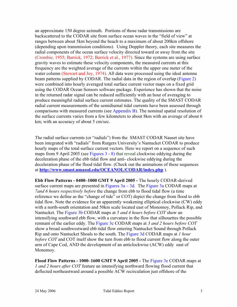
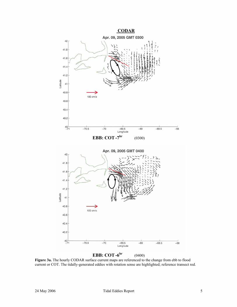
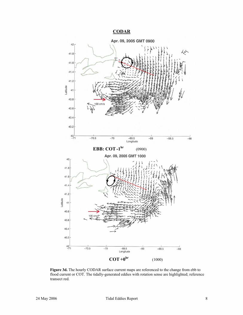
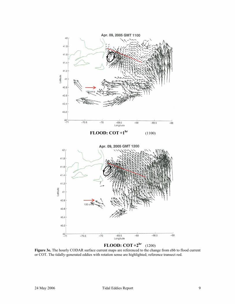
an approximate 150 degree azimuth. Portions of those radar transmissions are backscattered to the CODAR site from surface ocean waves in the “field of view” at ranges between about 5km beyond the beach to a maximum of about 200km offshore (depending upon transmission conditions). Using Doppler theory, each site measures the radial components of the ocean surface velocity directed toward or away from the site (Crombie, 1955; Barrick, 1972; Barrick et al., 1977). Since the systems are using surface gravity waves to estimate these velocity components, the measured currents at this frequency are the weighted average of the currents within the upper one meter of the water column (Stewart and Joy, 1974). All data were processed using the ideal antenna beam patterns supplied by CODAR. The radial data in the region of overlap (Figure 2) were combined into hourly averaged total surface current vector maps on a fixed grid using the CODAR Ocean Sensors software package. Experience has shown that the noise in the returned radar signal can be reduced sufficiently with an hour of averaging to produce meaningful radial surface current estimates. The quality of the SMAST CODAR radial current measurements of the semidiurnal tidal currents have been assessed through comparisons with measured currents (see Appendix B). The nominal spatial resolution of the surface currents varies from a few kilometers to about 8km with an average of about 6 km; with an accuracy of about 5 cm/sec. The radial surface currents (or “radials”) from the SMAST CODAR Nauset site have been integrated with “radials” from Rutgers University’s Nantucket CODAR to produce hourly maps of the total surface current vectors. Here we report on a sequence of such maps from 9 April 2005 (see Figures 3 - 8) that reveal clockwise eddying during the deceleration phase of the ebb tidal flow and anti- clockwise eddying during the deceleration phase of the flood tidal flow. (Check out the animations of these sequences at http://www.smast.umassd.edu/OCEANOL/CODAR/index.php ). Ebb Flow Patterns - 0400–1000 GMT 9 April 2005 - The hourly CODAR-derived surface current maps are presented in Figures 3a – 3d. The Figure 3a CODAR maps at 7and 6 hours respectively before the change from ebb to flood tidal flow (a time reference we define as the “change of tide” or COT) depict the change from flood to ebb tidal flow. Note the evidence for an apparently weakening elliptical clockwise (CW) eddy with a north-south orientation and 50km scale located east of Monomoy, Pollack Rip, and Nantucket. The Figure 3b CODAR maps at 5 and 4 hours before COT show an intensifying southward ebb flow, with a curvature in the flow that silhouettes the possible remnant of the earlier eddy. The Figure 3c CODAR maps at 3 and 2 hours before COT show a broad southwestward ebb tidal flow entering Nantucket Sound through Pollack Rip and onto Nantucket Shoals to the south. The Figure 3d CODAR maps at 1 hour before COT and COT itself show the turn from ebb to flood current flow along the outer arm of Cape Cod, AND the development of an anticlockwise (ACW) eddy east of Monomoy. Flood Flow Patterns - 1000–1600 GMT 9 April 2005 - The Figure 3e CODAR maps at 1 and 2 hours after COT feature an intensifying northward flowing flood current that deflected northeastward around a possible ACW recirculation just offshore of the

24 May 2006 Tidal Eddies Report 4
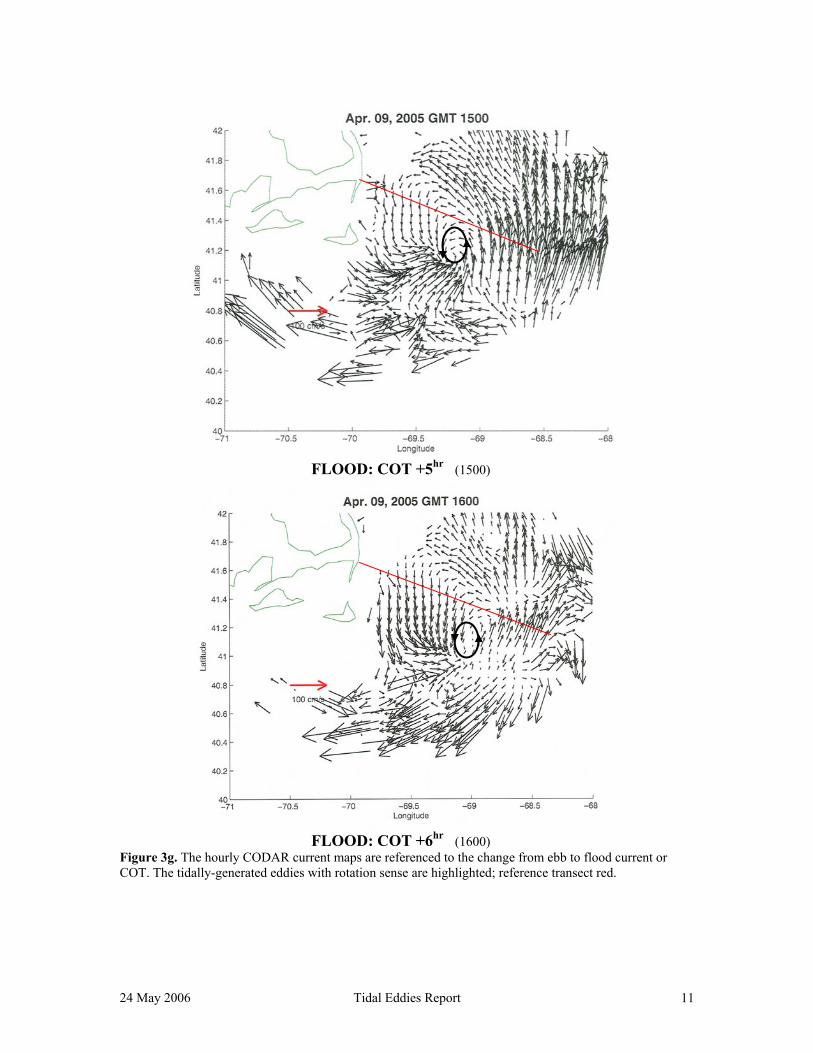
Monomoy coast. The Figure 3f CODAR maps at 3 and 4 hours after COT feature a weakening northward flowing flood current that too is deflected ACW around a more well-defined eddy just offshore of Monomoy. The 1400 GMT map indicates some offshore translation of the eddy. The Figure 3fg CODAR maps at 5 and 6 hours after COT feature a further offshore translation of the eddy at a rate of about 20km per hour.
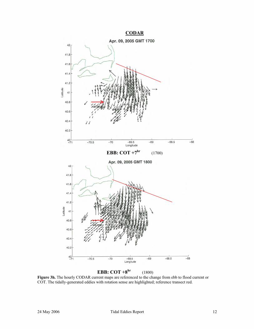
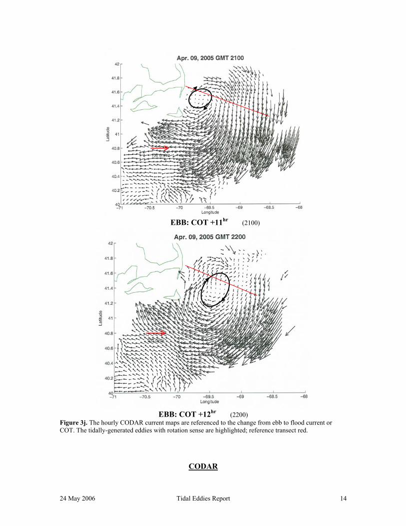
Figure 2. A schematic of CODAR radials from the Nauset and the Nantucket CODAR sites. The nominal spatial resolution of the CODAR surface currents is 6km. The “reference transect” for locating the tidal eddies (bold line) and the 100m (dot-dash) and 200m (dotted) isobaths are indicated Ebb Flow Patterns -1600–2200 GMT 9 April 2005 - The Figure 3h CODAR maps at 7and 8 hours after COT (5 and 4 hours before the next COT) show an intensifying southward ebb flow from the western Gulf of Maine onto Nantucket Shoals. The Figure 3i CODAR maps at 9 and 10 hours after COT (3 and 2 hours before the next COT) show an intensifying southward ebb flow, with a curvature in the flow that silhouettes a possibly growing CW eddy just offshore of Monomoy. The Figure 3j CODAR map at 11 after COT (about 11/2 hours before the next COT) features a 20km-scale elliptical eddy east of Monomoy that in the next hour moves offshore about 20km along the reference transect and grows to about 50km in size – all silhouetted by a broad and weakening southwestward ebb tidal flow onto Nantucket Shoals. The Figure 3k CODAR maps at about 13 hour after COT (the next COT) features the turn from ebb to flood current flow along the outer arm of Cape Cod, AND the disappearance of the eddy.. The eddies seen in these CODAR surface current maps are mimicked in the model simulations of semidiurnal tide as described next.
24 May 2006 Tidal Eddies Report 5
CODAR
EBB: COT -7hr (0300)
EBB: COT -6hr (0400)
Figure 3a. The hourly CODAR surface current maps are referenced to the change from ebb to flood current or COT. The tidally-generated eddies with rotation sense are highlighted; reference transect red.
24 May 2006 Tidal Eddies Report 6
CODAR
EBB: COT -5hr (0500)
EBB: COT -4hr (0600)
Figure 3b. The hourly CODAR surface current maps are referenced to the change from ebb to flood current or COT. The tidally-generated eddies with rotation sense are highlighted; reference transect is red.
CODAR

24 May 2006 Tidal Eddies Report 7
EBB: COT -3hr (0700)
EBB: COT -2hr (0800)
Figure 3c. The hourly CODAR surface current maps are referenced to the change from ebb to flood current or COT. The tidally-generated eddies with rotation sense are highlighted; reference transect red.
24 May 2006 Tidal Eddies Report 8
CODAR
EBB: COT -1hr (0900)
COT +0hr (1000)
Figure 3d. The hourly CODAR surface current maps are referenced to the change from ebb to flood current or COT. The tidally-generated eddies with rotation sense are highlighted; reference transect red.
24 May 2006 Tidal Eddies Report 9
FLOOD: COT +1hr (1100)
FLOOD: COT +2hr (1200)
Figure 3e. The hourly CODAR surface current maps are referenced to the change from ebb to flood current or COT. The tidally-generated eddies with rotation sense are highlighted; reference transect red.

24 May 2006 Tidal Eddies Report 10
CODAR
FLOOD: COT +3hr (1300)
FLOOD: COT +4hr (1400)
Figure 3f. The hourly CODAR current maps are referenced to the change from ebb to flood current or COT. The tidally-generated eddies with rotation sense are highlighted; reference transect red.
CODAR
24 May 2006 Tidal Eddies Report 11
FLOOD: COT +5hr (1500)
FLOOD: COT +6hr (1600)
Figure 3g. The hourly CODAR current maps are referenced to the change from ebb to flood current or COT. The tidally-generated eddies with rotation sense are highlighted; reference transect red.
24 May 2006 Tidal Eddies Report 12
CODAR
EBB: COT +7hr (1700)
EBB: COT +8hr (1800)
Figure 3h. The hourly CODAR current maps are referenced to the change from ebb to flood current or COT. The tidally-generated eddies with rotation sense are highlighted; reference transect red.

24 May 2006 Tidal Eddies Report 13
CODAR
EBB: COT +9hr (1900)
EBB: COT +10hr (2000)
Figure 3i. The hourly CODAR current maps are referenced to the change from ebb to flood current or COT. The tidally-generated eddies with rotation sense are highlighted; reference transect red.
CODAR
24 May 2006 Tidal Eddies Report 14
EBB: COT +11hr (2100)
EBB: COT +12hr (2200)
Figure 3j. The hourly CODAR current maps are referenced to the change from ebb to flood current or COT. The tidally-generated eddies with rotation sense are highlighted; reference transect red.
CODAR

24 May 2006 Tidal Eddies Report 15
COT +13hr (2300)
Figure 3k. The hourly CODAR current maps are referenced to the change from ebb to flood current or COT. The tidally-generated eddies with rotation sense are highlighted; reference transect red.
3. The Modeling To simulate the semidiurnal tidal currents in the region of the CODAR coverage (see Figure 1, we used the Lynch et al. (1996, 1997) finite-element coastal ocean circulation model QUODDY in its barotropic (i.e. uniform density) mode with just M2 semidiurnal tidal sea level forcing. The model domain is defined by the Holboke (1998) GHSD unstructured mesh, with a lateral resolution that varies from about 10 km in the interior of the Gulf to about 5 km near the coastlines; with even finer resolution in the regions of steep bathymetric slopes, such as the north flank of Georges Bank. There are 21 sigma layers vertically. A 10-m minimum depth was adopted for the coastal boundary elements. The model results considered here were produced every 1/16th M2 tidal cycle for the 9-10 April 2005 time period of the CODAR observations. (See Appendix A for more details regarding the model setup and run). The accuracy of the QUODDY model M2 tidal sea level results was assessed through a comparison with the Moody et al. (1984) M2 tidal sea level harmonic constants derived from sea level measurements at the 49 locations in the model domain (see Table A1). For stations in the Gulf of Maine and on Georges Ban, the observed and model M2 tidal sea level amplitude differences are typically within 10% of each other; with phase differences typically within 10 degrees of each other. This high quality fit between model

24 May 2006 Tidal Eddies Report 16
and observed M2 tidal sea level at stations on the seaward side of Cape Cod and Nantucket Shoals is particularly relevant to the eddy generation and evolution process considered here. Model Surface Currents: The model current simulation results in Figures 4a-p cover one full M2 tidal cycle at 16th M2 tidal intervals starting just after the change from flood to ebb current in the western Great South Channel. The model surface current results are referenced to the change of tide (COT) configuration at 1000 GMT 9 April 2005 (Figure 4i) when (by definition) the ebb tidal flow changed to flood tidal flow in the Great South Channel. The remnants of a flood current-generated eddy (Figure 4a) disintegrate as the tidal flow changes from flood to ebb (Figure 4b). Model Ebb Flow Eddy Generation: The model M2 tidal coastal ebb flow separation and eddy generation process at the elbow Cape Cod is depicted in Figures 4c-g). The sequence of model surface flow maps (a) starts [at COT -4.67hr (99)] with smooth along-coast flow toward Nantucket Shoals (Figure 4c ); (b) followed [at COT-3.89hr (100)] with the beginnings of the separation of the along-coast flow from the coast (Figure 4d); (c) followed [at COT-3.11hr (101)] by even more separation of the along-coast flow (Figure 4e); (d) followed [at COT-2.33hr (102)] by a “full” flow separation zone (Figure 4f); in which (e) a small clockwise eddy is formed [at COT-1.55hr (103)] (Figure 4g). Model Ebb Flow Eddy Translation: Over the next few maps from COT-0.78hr (104) through COT+0.78hr (106), (Figures 4h-j). respectively) the eddy translated eastward generally along the transect to an area about 80 km offshore where it lost its identity in the throes of the change from ebb to flood tide. The center of the eddy is located in the transect distributions of the normal, lateral and upward model current fields shown in those figures.

24 May 2006 Tidal Eddies Report 17
MODEL
Figure 4a The model M2 tidal surface current pattern for the change from flood tidal flow to ebb flow at COT -6.21hr (097), where COT refers to the change from ebb to flood tidal flow at 1000 GMT 9 April 2005. (top) A remnant of a flood flow-generated anticlockwise eddy is highlighted and the reference transect (see text) and current scale are indicated (red); (middle left) northward flow - approximately normal the reference transect; (middle right) eastward flow; (bottom) upward flow; current speed (cm/s) legend is to right.
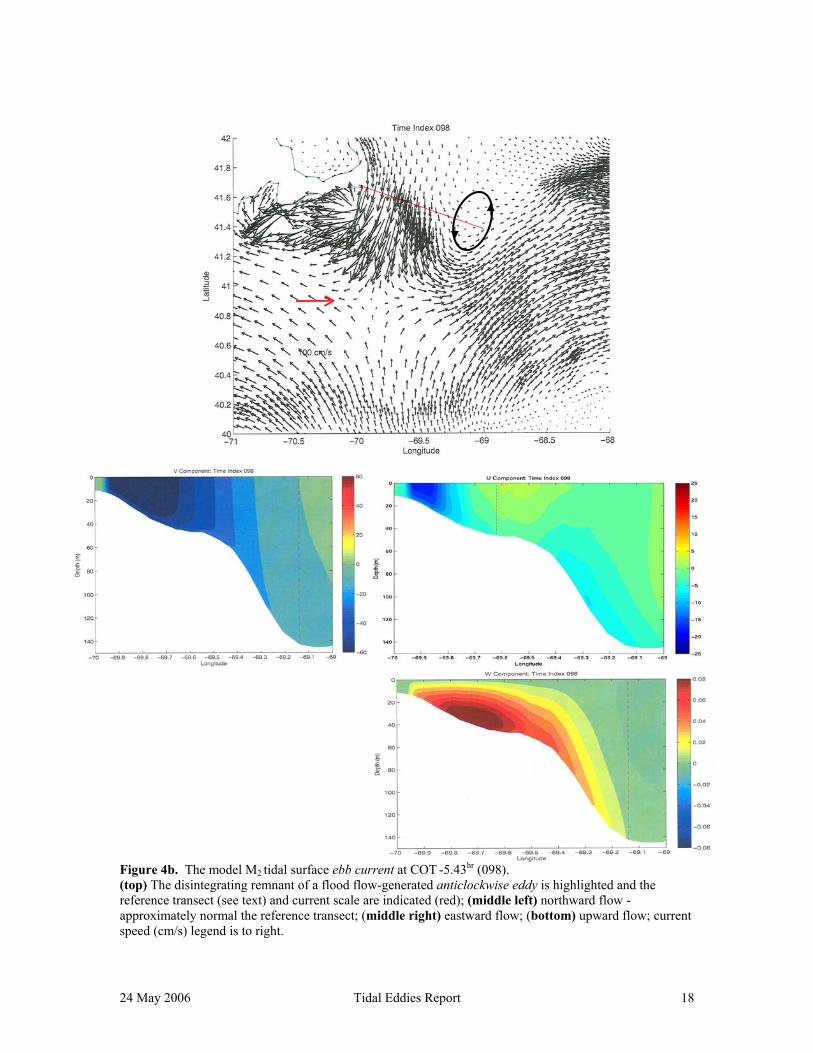
24 May 2006 Tidal Eddies Report 18
Figure 4b. The model M2 tidal surface ebb current at COT -5.43hr (098). (top) The disintegrating remnant of a flood flow-generated anticlockwise eddy is highlighted and the reference transect (see text) and current scale are indicated (red); (middle left) northward flow - approximately normal the reference transect; (middle right) eastward flow; (bottom) upward flow; current speed (cm/s) legend is to right.

24 May 2006 Tidal Eddies Report 19
MODEL
Figure 4c. The model M2 tidal surface ebb current at COT -4.66hr (099). (top) An accelerating ebb flow, with the reference transect (see text) and current scale are indicated (red); (middle left) northward flow - approximately normal the reference transect; (middle right) eastward flow; (bottom) upward flow; current speed (cm/s) legend is to right.
24 May 2006 Tidal Eddies Report 20
MODEL
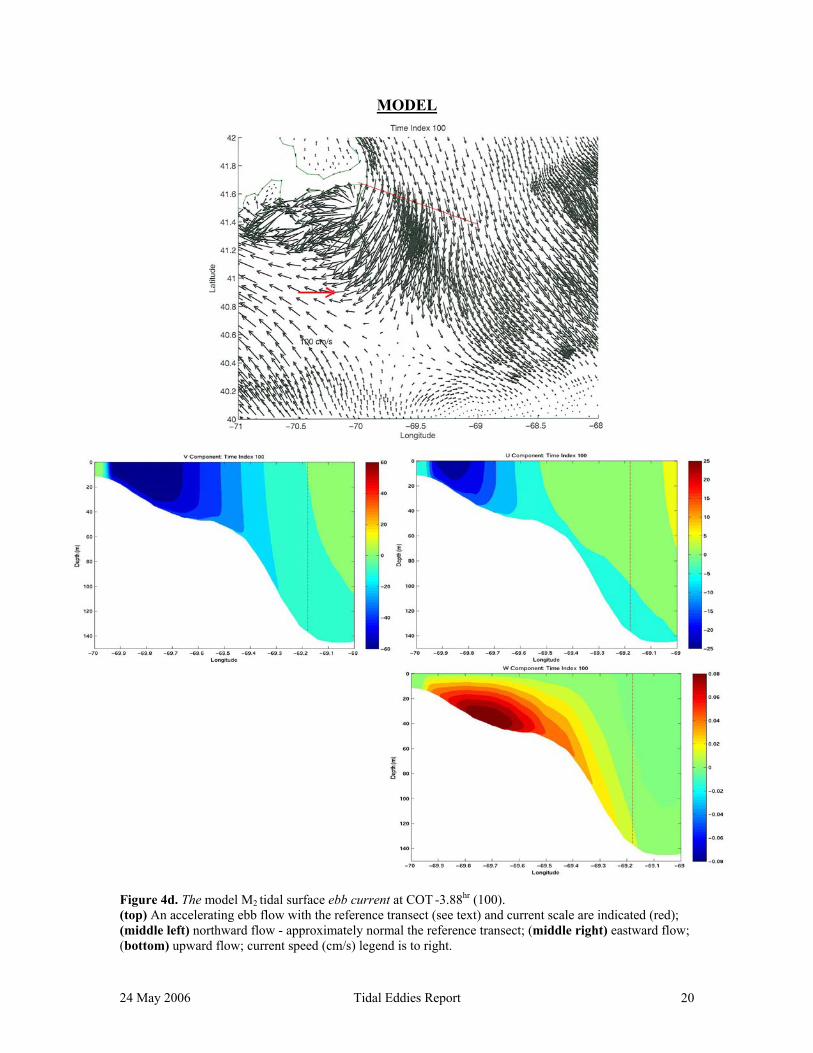
Figure 4d. The model M2 tidal surface ebb current at COT -3.88hr (100). (top) An accelerating ebb flow with the reference transect (see text) and current scale are indicated (red); (middle left) northward flow - approximately normal the reference transect; (middle right) eastward flow; (bottom) upward flow; current speed (cm/s) legend is to right.

24 May 2006 Tidal Eddies Report 21
MODEL
Figure 4e. The model M2 tidal surface ebb current at COT -3.11hr (101). (top) An ebb flow that is beginning to separate from the coast near the elbow of Cape Cod, with the reference transect (see text) and current scale are indicated (red); (middle left) northward flow - approximately normal the reference transect; (middle right) eastward flow; (bottom) upward flow; current speed (cm/s) legend is to right.

24 May 2006 Tidal Eddies Report 22
MODEL
Figure 4f The model M2 tidal surface ebb current at COT -2.33hr (102). (top) A separation of the decelerating ebb flow is even more pronounced than in the previous map, on which the reference transect (see text) and current scale are indicated (red); (middle left) northward flow - approximately normal the reference transect; (middle right) eastward flow; (bottom) upward flow; current speed (cm/s) legend is to right.

24 May 2006 Tidal Eddies Report 23
MODEL
Figure 4g. The model M2 tidal surface ebb current at COT -1.55hr (103). (top) An ebb flow-generated clockwise eddy appears on this map, on which the reference transect (see text) and current scale are indicated (red); (middle left) northward flow - approximately normal the reference transect; (middle right) eastward flow; (bottom) upward flow; current speed (cm/s) legend is to right.
24 May 2006 Tidal Eddies Report 24
MODEL
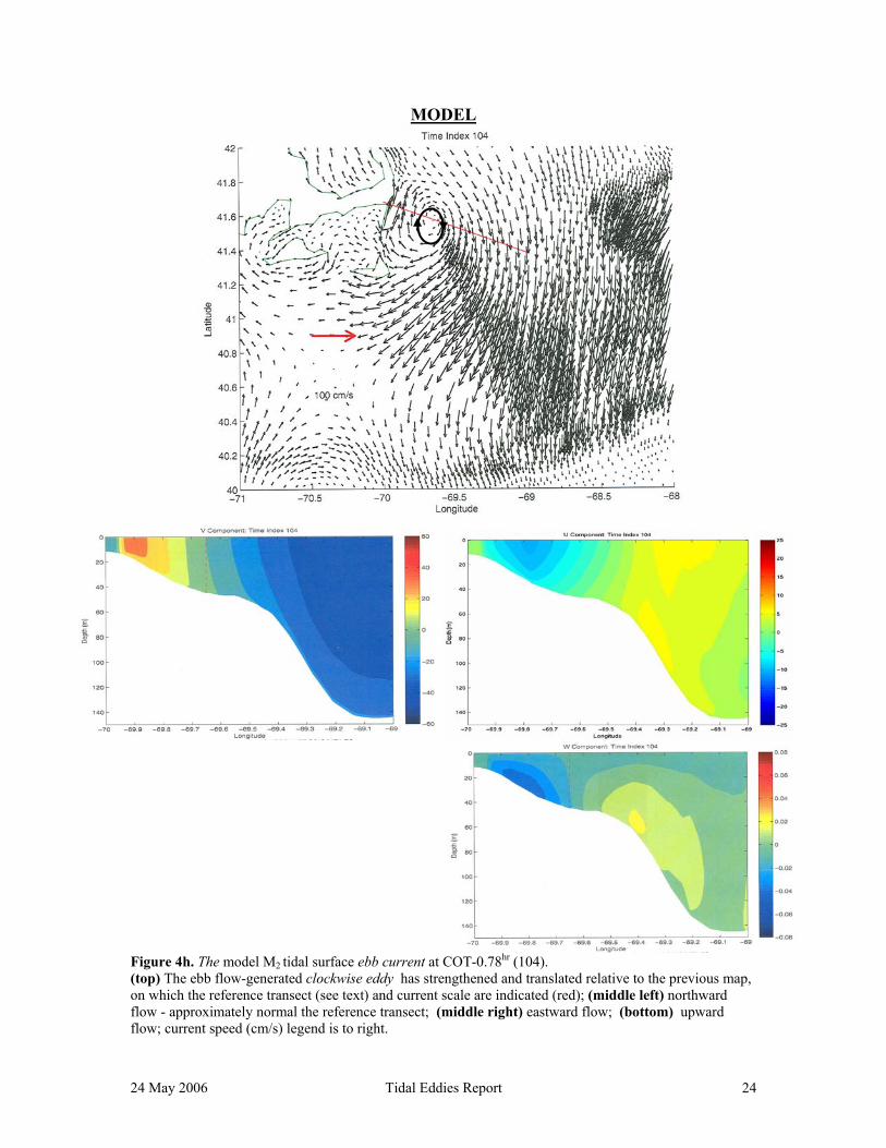
Figure 4h. The model M2 tidal surface ebb current at COT-0.78hr (104). (top) The ebb flow-generated clockwise eddy has strengthened and translated relative to the previous map, on which the reference transect (see text) and current scale are indicated (red); (middle left) northward flow - approximately normal the reference transect; (middle right) eastward flow; (bottom) upward flow; current speed (cm/s) legend is to right.

24 May 2006 Tidal Eddies Report 25
MODEL
Figure 4i. The model M2 tidal surface current at the “change of tide” COT+ 0.00hr (105). (top) The ebb flow-generated clockwise eddy has weakened relative to the previous amp, on which on the reference transect (see text) and current scale are indicated (red); (middle left) northward flow - approximately normal the reference transect; (middle right) eastward flow; (bottom) upward flow; current speed (cm/s) legend is to right.

24 May 2006 Tidal Eddies Report 26
MODEL
Figure 4j. The model M2 tidal surface flood current at COT+0.78hr (106). (top) The remnant ebb flow-generated clockwise eddy is disintegrating on this amp, on which the reference transect (see text) and current scale are indicated (red); (middle left) northward flow - approximately normal the reference transect; (middle right) eastward flow; (bottom) upward flow; current speed (cm/s) legend is to right.

24 May 2006 Tidal Eddies Report 27
MODEL
Figure 4k. The model M2 tidal surface flood current at COT +1.55hr (107). (top) Flood flow, with the reference transect (see text) and current scale are indicated (red); (middle left) northward flow - approximately normal the reference transect; (middle right) eastward flow; (bottom) upward flow; current speed (cm/s) legend is to right.

24 May 2006 Tidal Eddies Report 28
MODEL
Figure 4l. The model M2 tidal surface flood current at COT +2.33hr (108). (top) Flood flow, with the reference transect (see text) and current scale are indicated (red); (middle left) northward flow - approximately normal the reference transect; (middle right) eastward flow; (bottom) upward flow; current speed (cm/s) legend is to right.

24 May 2006 Tidal Eddies Report 29
MODEL
Figure 4m. The model M2 tidal surface flood current at COT +3.11hr (109). (top) The flood flow shows signs of separation from the coast on this map, on which the reference transect (see text) and current scale are indicated (red); (middle left) northward flow - approximately normal the reference transect; (middle right) eastward flow; (bottom) upward flow; current speed (cm/s) legend is to right.

24 May 2006 Tidal Eddies Report 30
MODEL
Figure 4n. The model M2 tidal surface flood current at COT +3.88hr (110). (top) A flood flow-generated anticlockwise eddy appears near the coast on this map, on which and the reference transect (see text) and current scale are indicated (red); (middle left) northward flow - approximately normal the reference transect; (middle right) eastward flow; (bottom) upward flow; current speed (cm/s) legend is to right.

24 May 2006 Tidal Eddies Report 31
MODEL
Figure 4o. The model M2 tidal surface flood current at COT +4.66hr (111). (top) The flood flow-generated anticlockwise eddy has strengthened and translated seaward relative to the previous map, on which and the reference transect (see text) and current scale are indicated (red); (middle left) northward flow - approximately normal the reference transect; (middle right) eastward flow; (bottom) upward flow; current speed (cm/s) legend is to right.

24 May 2006 Tidal Eddies Report 32
MODEL
Figure 4p. The model M2 tidal surface flood current at COT +5.43hr (112) (096). (top) The flood flow-generated anticlockwise eddy has weakened and translated relative to the previous map, on which the reference transect (see text) and current scale are indicated (red); (middle left) northward flow - approximately normal the reference transect; (middle right) eastward flow; (bottom) upward flow; current speed (cm/s) legend is to right.

24 May 2006 Tidal Eddies Report 33
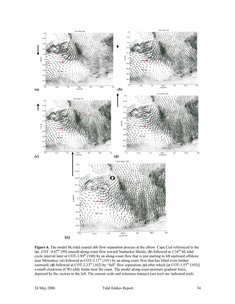
4. Model Ebb Flow Eddy Production The conceptual model underlying the generation of transient coastal eddies involves adverse along-coast pressure gradients that stall the along-coast boundary layer flow (see Signell and Geyer, 1991; Appendix C) and lead to flow separation from the coast. We extracted a proxy for the along-coast pressure gradient by differencing the sea levels at model nodes at Nauset and the tip of Monomoy Island (Figure 5). These pressure differences are included in the Figure 6a-f sequence of maps that depict the model M2 ebb flow separation and eddy generation process at the elbow Cape Cod. Note that the model along-coast pressure gradient force between Nauset and the tip of Monomoy (see Figure 5) becomes “adverse” with the first hint of flow separation in Figure 6b and increases in magnitude as time advances. The sequence (a) starts at COT -4.67hr (99) with smooth along-coast flow toward Nantucket Shoals (Figure 6a), where COT is the time (1000 GMT 9 April 2005) of the change from ebb to flood tidal flow in this location; (b) followed at COT-3.89hr (100) with the hint of the separation of the along-coast flow from the coast (Figure 6b); (c) followed at COT-3.11hr (101) by an identifiable separation of the along-coast flow (Figure 6c); (d) followed at COT-2.33hr (102) by a “full” flow separation zone (Figure 6d); and (e) finally at COT-1.55hr (103) by the appearance a small clockwise eddy (Figure 6e).
Figure 5. The QUODDY sea level nodes at Nauset and Monomoy used to compute along-coast pressure difference. Model Ebb Flow Eddy Translation: Over the next few maps from COT-0.78hr (104) through COT+0.78hr (106), (Figures 4h, 4i, and 4j respectively) the eddy translated eastward generally along the transect to an area about 80 km offshore where it lost its identity in the throes of the change from ebb to flood tide. The center of the eddy is located in the transect distributions of the normal, lateral and upward model current fields shown in those figures.
24 May 2006 Tidal Eddies Report 34
(a) (b)
(c) (d)
(e)
Figure 6. The model M2 tidal coastal ebb flow separation process at the elbow Cape Cod referenced to the (a) COT -4.67hr (99) smooth along-coast flow toward Nantucket Shoals; (b) followed at 1/16th M2 tidal cycle interval later or COT-3.89hr (100) by an along-coast flow that is just starting to lift eastward offshore near Monomoy; (c) followed at COT-3.11hr (101) by an along-coast flow that has lifted even further eastward; (d) followed at COT-2.33hr (102) by “full” flow separation; (e) after which [at COT-1.55hr (103)] a small clockwise (CW) eddy forms near the coast. The model along-coast pressure gradient force, depicted by the vectors to the left. The current scale and reference transect (see text) are indicated (red).
24 May 2006 Tidal Eddies Report 35
5. Acknowledgements The SMAST measurements that helped to define these transient eddies would never been made if not for the leadership and effort of Glenn Strout and technical assistance of Rob Fisher in the original installation of the equipment. The ongoing support and assistance of J. Kohut and S. Glenn (School for Maine Science & Technology, Rutgers University) has been invaluable to the installation and maintenance of our CODAR. Of course the Rutgers group operates and maintains the Nantucket CODAR, with which we partner. The SMAST CODAR is deployed at the US National Park Service’s Cape Cod National Seashore station in Eastham, MA. A US Dept of Education FIPSE grant (2002) and NASA Contract NAG 13-02042 have supported this effort.

24 May 2006 Tidal Eddies Report 36
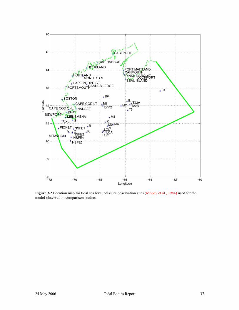
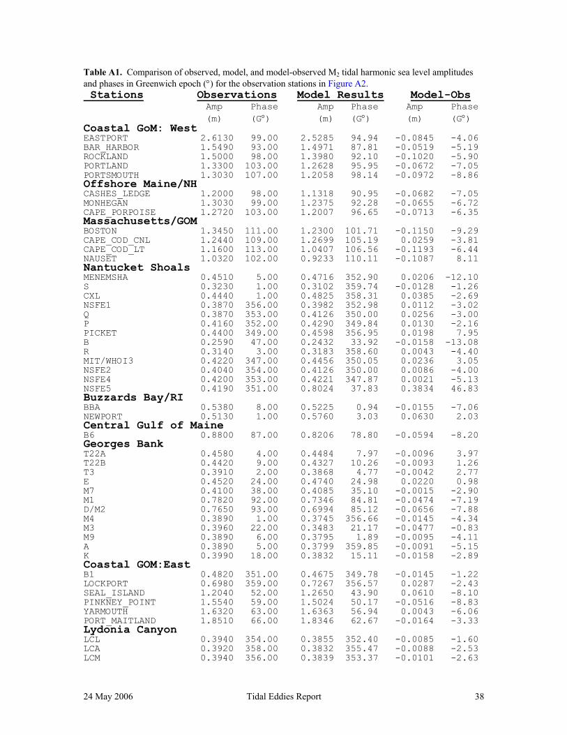
APPENDIX A. Barotropic M2-Only Tidal Forced Ocean Modeling Model Description: QUODDY is a 3-D, nonlinear, prognostic, f-plane, finite-element coastal ocean circulation model with advanced turbulence closure (Lynch et al., 1996, 1997). In this application, bottom flow bV is subject to quadratic bottom boundary stress, according to bbd VVC || , where the time/space constant bottom drag coefficient dC is 0.005. There was no surface forcing for this study. The QUODDY model domain (see Figure 1 in main text) is defined by the Holboke (1998) GHSD mesh. The mesh resolution varies from about 10 km in the gulf to about 5 km near the coastlines with even finer resolution in the regions of steep bathymetric slopes like the north flank Georges Bank. A 10-m minimum depth was adopted for the coastal boundary elements. Vertically here are 21 sigma layers. The conditions imposed on the different QUODDY open ocean boundaries are: Deep Ocean and Western Cross-Shelf Sections (red line; Figure A1): The predicted semidiurnal M2 tidal elevation forcing, zero steady residual or non-tidal elevation, and the Holboke (1998) inhomogeneous and barotropic radiation conditions; Bay of Fundy Section (black line; Figure A1)): The predicted M2, M4, M6 normal flow, constrained by a condition of zero non-tidal transport normal to the section; and Cross-Shelf Section at Halifax (blue line; Figure A1)): The predicted M2 tidal elevations, a zero steady residual elevation, and the Holboke (1998) inhomogeneous and barotropic radiation boundary conditions. The model was initialized with zero velocity and elevation fields for this barotropic calculation, which employed homogeneous water density. So that the model nonlinearities and advection could dynamically adjust to the initial fields (Holboke, 1998), the prescribed M2 tidal sea level forcing-only (due to Lynch et al., 1997) was linearly increased to full forcing (i.e. ramped-up) during the first six 2M tidal cycles. Holboke (1998) has shown with QUODDY runs with a similar model configuration reach dynamical equilibrium after 6 tidal cycles. After ramp-up, the model was run with a 21.83203125 second (= the 12.42-hour 2M tidal period/2048) time-step for 2 additional M2 tidal cycles. Model/Observation Comparisons: Model sea level time series were extracted at the 49 nodes which were nearest to the corresponding Moody et al. (1984) observation stations (Figure A2). Then the 2 M2 tidal cycle series were joined end-to-end to produce 2-month time series at each of the 49 sites. The M2 tidal sea level harmonic constants for each of the model stations are compared in Table A1with those from Moody et al. (1984). For stations in the Gulf of Maine and on Georges Bank, the observed and model M2 tidal sea level amplitude differences are typically within 10% of each other; with corresponding phase differences typically within 10 degrees of each other.
24 May 2006 Tidal Eddies Report 37
Figure A2 Location map for tidal sea level pressure observation sites (Moody et al., 1984) used for the model-observation comparison studies.
24 May 2006 Tidal Eddies Report 38
Table A1. Comparison of observed, model, and model-observed M2 tidal harmonic sea level amplitudes and phases in Greenwich epoch (°) for the observation stations in Figure A2. Stations Observations Model Results Model-Obs
Amp Phase Amp Phase Amp Phase (m) (G°) (m) (G°) (m) (G°) Coastal GoM: West
EASTPORT 2.6130 99.00 2.5285 94.94 -0.0845 -4.06 BAR_HARBOR 1.5490 93.00 1.4971 87.81 -0.0519 -5.19 ROCKLAND 1.5000 98.00 1.3980 92.10 -0.1020 -5.90 PORTLAND 1.3300 103.00 1.2628 95.95 -0.0672 -7.05 PORTSMOUTH 1.3030 107.00 1.2058 98.14 -0.0972 -8.86 Offshore Maine/NH CASHES_LEDGE 1.2000 98.00 1.1318 90.95 -0.0682 -7.05 MONHEGAN 1.3030 99.00 1.2375 92.28 -0.0655 -6.72 CAPE_PORPOISE 1.2720 103.00 1.2007 96.65 -0.0713 -6.35 Massachusetts/GOM BOSTON 1.3450 111.00 1.2300 101.71 -0.1150 -9.29 CAPE_COD_CNL 1.2440 109.00 1.2699 105.19 0.0259 -3.81 CAPE_COD_LT 1.1600 113.00 1.0407 106.56 -0.1193 -6.44 NAUSET 1.0320 102.00 0.9233 110.11 -0.1087 8.11 Nantucket Shoals MENEMSHA 0.4510 5.00 0.4716 352.90 0.0206 -12.10 S 0.3230 1.00 0.3102 359.74 -0.0128 -1.26 CXL 0.4440 1.00 0.4825 358.31 0.0385 -2.69 NSFE1 0.3870 356.00 0.3982 352.98 0.0112 -3.02 Q 0.3870 353.00 0.4126 350.00 0.0256 -3.00 P 0.4160 352.00 0.4290 349.84 0.0130 -2.16 PICKET 0.4400 349.00 0.4598 356.95 0.0198 7.95 B 0.2590 47.00 0.2432 33.92 -0.0158 -13.08 R 0.3140 3.00 0.3183 358.60 0.0043 -4.40 MIT/WHOI3 0.4220 347.00 0.4456 350.05 0.0236 3.05 NSFE2 0.4040 354.00 0.4126 350.00 0.0086 -4.00 NSFE4 0.4200 353.00 0.4221 347.87 0.0021 -5.13 NSFE5 0.4190 351.00 0.8024 37.83 0.3834 46.83 Buzzards Bay/RI BBA 0.5380 8.00 0.5225 0.94 -0.0155 -7.06 NEWPORT 0.5130 1.00 0.5760 3.03 0.0630 2.03 Central Gulf of Maine B6 0.8800 87.00 0.8206 78.80 -0.0594 -8.20 Georges Bank T22A 0.4580 4.00 0.4484 7.97 -0.0096 3.97 T22B 0.4420 9.00 0.4327 10.26 -0.0093 1.26 T3 0.3910 2.00 0.3868 4.77 -0.0042 2.77 E 0.4520 24.00 0.4740 24.98 0.0220 0.98 M7 0.4100 38.00 0.4085 35.10 -0.0015 -2.90 M1 0.7820 92.00 0.7346 84.81 -0.0474 -7.19 D/M2 0.7650 93.00 0.6994 85.12 -0.0656 -7.88 M4 0.3890 1.00 0.3745 356.66 -0.0145 -4.34 M3 0.3960 22.00 0.3483 21.17 -0.0477 -0.83 M9 0.3890 6.00 0.3795 1.89 -0.0095 -4.11 A 0.3890 5.00 0.3799 359.85 -0.0091 -5.15 K 0.3990 18.00 0.3832 15.11 -0.0158 -2.89 Coastal GOM:East B1 0.4820 351.00 0.4675 349.78 -0.0145 -1.22 LOCKPORT 0.6980 359.00 0.7267 356.57 0.0287 -2.43 SEAL_ISLAND 1.2040 52.00 1.2650 43.90 0.0610 -8.10 PINKNEY_POINT 1.5540 59.00 1.5024 50.17 -0.0516 -8.83 YARMOUTH 1.6320 63.00 1.6363 56.94 0.0043 -6.06 PORT_MAITLAND 1.8510 66.00 1.8346 62.67 -0.0164 -3.33 Lydonia Canyon LCL 0.3940 354.00 0.3855 352.40 -0.0085 -1.60 LCA 0.3920 358.00 0.3832 355.47 -0.0088 -2.53 LCM 0.3940 356.00 0.3839 353.37 -0.0101 -2.63
24 May 2006 Tidal Eddies Report 39
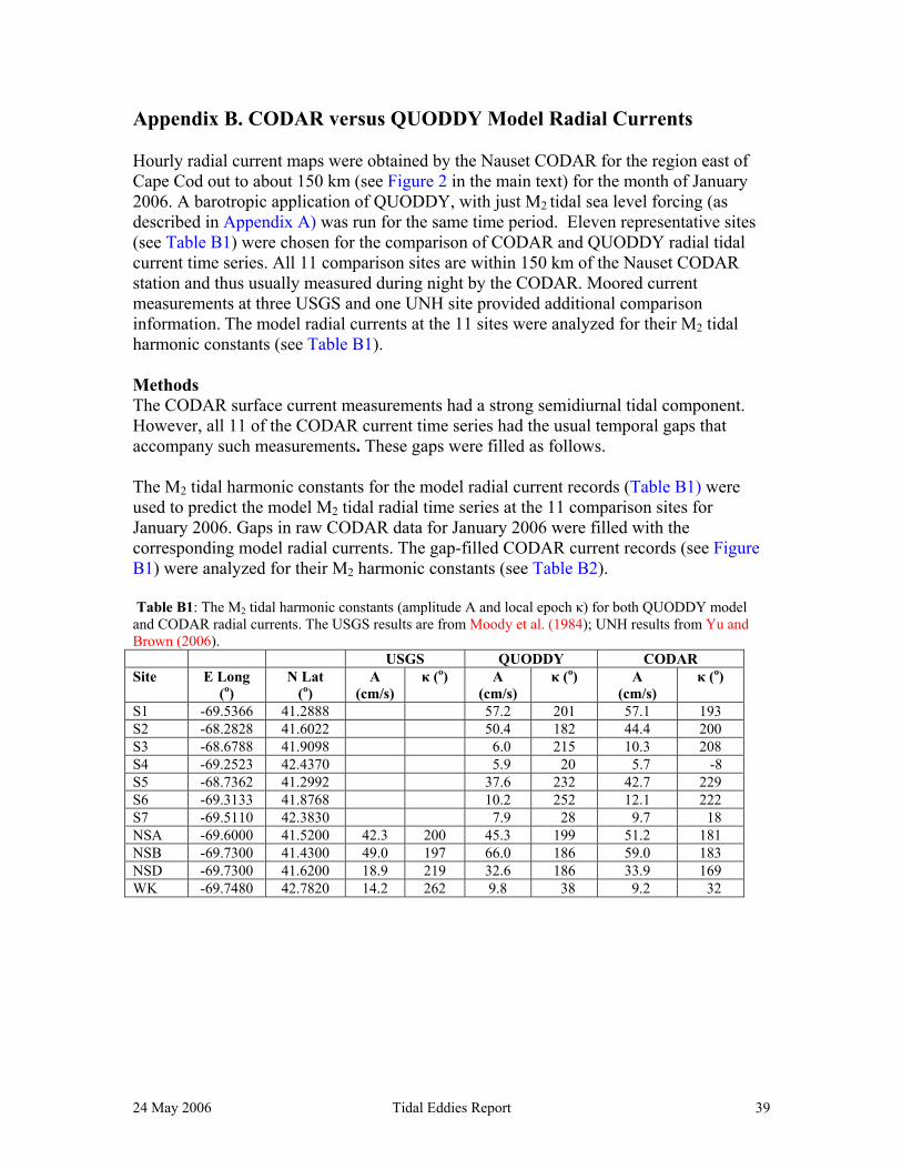
Appendix B. CODAR versus QUODDY Model Radial Currents Hourly radial current maps were obtained by the Nauset CODAR for the region east of Cape Cod out to about 150 km (see Figure 2 in the main text) for the month of January 2006. A barotropic application of QUODDY, with just M2 tidal sea level forcing (as described in Appendix A) was run for the same time period. Eleven representative sites (see Table B1) were chosen for the comparison of CODAR and QUODDY radial tidal current time series. All 11 comparison sites are within 150 km of the Nauset CODAR station and thus usually measured during night by the CODAR. Moored current measurements at three USGS and one UNH site provided additional comparison information. The model radial currents at the 11 sites were analyzed for their M2 tidal harmonic constants (see Table B1). Methods The CODAR surface current measurements had a strong semidiurnal tidal component. However, all 11 of the CODAR current time series had the usual temporal gaps that accompany such measurements. These gaps were filled as follows. The M2 tidal harmonic constants for the model radial current records (Table B1) were used to predict the model M2 tidal radial time series at the 11 comparison sites for January 2006. Gaps in raw CODAR data for January 2006 were filled with the corresponding model radial currents. The gap-filled CODAR current records (see Figure B1) were analyzed for their M2 harmonic constants (see Table B2). Table B1: The M2 tidal harmonic constants (amplitude A and local epoch κ) for both QUODDY model and CODAR radial currents. The USGS results are from Moody et al. (1984); UNH results from Yu and Brown (2006). USGS QUODDY CODAR Site E Long
(o) N Lat
(o) A
(cm/s) κ (o) A
(cm/s) κ (o) A
(cm/s) κ (o)
S1 -69.5366 41.2888 57.2 201 57.1 193 S2 -68.2828 41.6022 50.4 182 44.4 200 S3 -68.6788 41.9098 6.0 215 10.3 208 S4 -69.2523 42.4370 5.9 20 5.7 -8 S5 -68.7362 41.2992 37.6 232 42.7 229 S6 -69.3133 41.8768 10.2 252 12.1 222 S7 -69.5110 42.3830 7.9 28 9.7 18 NSA -69.6000 41.5200 42.3 200 45.3 199 51.2 181 NSB -69.7300 41.4300 49.0 197 66.0 186 59.0 183 NSD -69.7300 41.6200 18.9 219 32.6 186 33.9 169 WK -69.7480 42.7820 14.2 262 9.8 38 9.2 32

24 May 2006 Tidal Eddies Report 40
−100
0
100
S1cm
/sQuoddy Results vs CODAR Raw Data
−100
0
100
S2cm
/s
−100
0
100
S3cm
/s
−100
0
100
S4cm
/s
−100
0
100
S5cm
/s
−100
0
100
S6cm
/s
−100
0
100
S7cm
/s
−100
0
100
NSAcm
/s
−100
0
100
NSBcm
/s
−100
0
100
NSDcm
/s
1 4 7 10 13 16 19 22 25 28−100
0
100
WLKcm
/s
January 2006 /hosts/iselin/data01/users/zyu/CODAR/RADs−TidalAnalysis−Jan−2006/MFILES
03−Feb−2006 13:58:15
−100
0
100
S1cm
/s
CODAR Raw Data Filled with Quoddy Results
−100
0
100
S2cm
/s
−100
0
100
S3cm
/s
−100
0
100
S4cm
/s
−100
0
100
S5cm
/s
−100
0
100
S6cm
/s
−100
0
100
S7cm
/s−100
0
100
NSAcm
/s
−100
0
100
NSBcm
/s
−100
0
100
NSDcm
/s
1 4 7 10 13 16 19 22 25 28−100
0
100
WLKcm
/s
January 2006 /hosts/iselin/data01/users/zyu/CODAR/RADs−TidalAnalysis−Jan−2006/MFILES
03−Feb−2006 13:59:22 Figure B1. (left) The M2 –only tidally-forced barotropic QUODDY radial currents (blue) for January 2006 and the model minus CODAR-derived radial current difference time series (red dash). (right) The gap-filled CODAR radial current records. Appendix C. Tidal Eddy Generation: Theoretical Considerations The theoretical framework for the transient eddies described here appears in Signell and Geyer (1991). We first outline those theoretical considerations and then show how they have relevance to the QUODDY model M2 tidally forced simulations. A. Theoretical Considerations Signell and Geyer (1991) describe the production, advection and dissipation of transient tidal eddies that are associated with coastal headlands in terms of the depth-averaged vorticity equation

24 May 2006 Tidal Eddies Report 41
A B C D
ωηωωω 2||∇+⋅
×∇−
∇⋅+∂∂+
=∇⋅+∂∂
HD Ak
HuuC
HutH
fut
rrrr ,
where u is the total velocity; H = h + η is total water depth with mean water depth h and sea level departure η ; yuxv ∂∂−∂∂= //ω is the vertical component of vorticity; CD
bottom drag coefficient; and AH horizontal eddy viscosity. In this expression, term A - the total change in vorticity following a fluid parcel - is balanced by vorticity production due to (term B) friction-free stretching or squashing and (term C) bottom friction torque respectively; plus (term D) diffusion due to horizontal mixing. The bottom friction torque vorticity production (term C), itself, has three components, namely
[ ]H
uCH
kuuCkHuH
uCkH
uuC DDDD ω|||)|(||||2
rrrr
rrr
+⋅∇×
−⋅∇×=⋅
×∇ ,
I II III which physically are the (I) “slope torque” vorticity production term in which the vertically-averaged flow normal to the bottom slope gradient “feels” different bottom friction; (II) “speed torque” vorticity production term in which stronger flow is retarded more than the weaker flow due to quadratic bottom stress; and (III) vorticity dissipation term due to bottom friction. In the vicinity of a coastal headland, there are offshore bathymetry gradients and often shear in the along-isobath flow (Robinson, 1981); thus allowing the production of generate vorticity from both slope torque and speed torque components. So how are eddies generated? In principle, vorticity can be generated by the no-slip coastal boundary condition (Tee, 1976), but the water depth goes to zero there. Thus that vorticity generation mechanism is difficult to distinguish from the bottom torque mechanism. Further, if the flow follows the coast, then the vorticity generated by these mechanisms does not reach the interior; and eddies are unlikely to form. However, Geyer and Signell (1991) measured transient eddies that formed as the semidiurnal tidal flow interacts with Gay Head Martha’s Vineyard, MA. and sought physical explanations. Signell and Geyer (1991) developed a coastal boundary layer separation model to explain how the along-coast flow in the vicinity of a headland spawns the observed transient eddies. The key physics in boundary layer separation is the along-coast change from a favoring along-coast pressure gradient to an adverse one that opposes the flow in the coastal boundary layer; and thus leads to offshore flow due to continuity. They describe how the nature of the transient eddy production process is characterized by a trio of non-dimensional parameters, namely the (1) headland geometry in terms of its aspect ratio α = b/a (with a = along-coast scale and b = cross-coast scale) ; (2) advection to friction ratio in terms of a Reynolds number Ref = [H/CDa] (Pingree and Maddock, 1980) ; and (3) advection to local acceleration ratio in terms of the Keulegan-Carpenter number Kc = [Uo /σa] , where Uo and σ are the tidal flow amplitude and frequency respectively. In their analysis anticlockwise (ACW) and
24 May 2006 Tidal Eddies Report 42
clockwise (CW) eddies are formed on alternating sides of the headland during ebb and flood tide respectively.
REFERENCES Barrick, D. E. (1972), First-order theory and analysis of mf/hf/vhf scatter from the sea, IEEE Trans.
Antennas Propag., AP-20, 2-10. Barrick, D. E., M. W. Evens, and B. L. Weber (1977), Ocean surface currents mapped by radar, Science,
198, 138-144. Battisti, D. S., and A. J. Clarke (1982), A simple method for estimating barotropic tidal currents on the
continental margins with specific application to the M2 tide off the Atlantic and Pacific coasts of the United States, J. Phys. Oceanogr., 12, 8-16.
Chapman, R. D., L. K. Shay, H. C. Graber, J. B. Edson, A. Karachintsev, C. L. Trump, and D. B. Ross (1997), On the accuracy of HF radar surface current measurements: Intercomparisons with ship-based sensors, J. Geophys. Res., 102, 18,737-18,748.
Crombie, D. D. (1955), Doppler spectrum of sea echo at 13.56 Mc/s, Nature, 175, 681-682. Erofeeva, S.Y., G. D. Egbert, and P. M. Kosro, 2003, Tidal currents on the central Oregon shelf: Models,
data, and assimilation, J. Geophys. Res., 108 (C5), 3148, doi:10.1029/2002JC0016l5. Gangopadhyay, A. C.Y. Shen, G.O. Marmorino, R.P. Mied and G.L. Lindemann, 2006. An extended
velocity projection method for estimating the subsurface current and density structure for coastal plume regions: An application to the Chesapeake Bay outflow plume, Cont. Shelf Res.(in press)
Geyer, W.R., and R. Signell, 1990. Measurements of tidal flow around a headland with a shipboard acoustic doppler current profiler, J. Geophys. Res., 95, 3189-3197.
Geyer, W.R., 1993. Three-Dimensional flow around headlands, J. Geophys. Res., 98, 955-966. Glenn, S. M., M. F. Crowley, D. B. Haidvogel, and Y. T. Song (1996), Underwater observatory captures
coastal upwelling events off New Jersey, Eos Trans. AGU, 77,233-236. Glenn, S. M., W. Boicourt, B. Parker, and T. D. Dickey (2000), Operational observation networks for ports,
a large estuary and an open shelf, Oceanography, 13, 12-23. Grassle, J. F., S. M. Glenn, and C. von Alt (1998), Ocean observing systems for marine habitats, OCC '98
Proceedings, Mar. Techno!. Soc., Baltimore, Md. Holboke, Monica J., 1998. “Variability of the Maine Coastal Current under Spring Conditions”, Ph.D.
Dissertation -Thayer School of Engineering -Dartmouth College, pp. 193. Kohut, J. T., and S. M. Glenn (2003), Improving HF radar surface current measurements with measured
antenna beam patterns, J. Atmos. Oceanic Technol.,20,1303-1316. Lynch, D. R., M. J. Holboke, and C.E. Naimie, 1997. The Maine coastal current: spring climatological
circulation. Continental Shelf Research, 17, 605-634. Lynch, D.R., J.T.C. Ip, C.E. Naimie, and F.E. Werner, 1996. Comprehensive coastal circulation model with
application to the Gulf of Maine. Continental Shelf Research, 16, 875-906. Moody, J., B. Butman, R.C. Beardsley, W.S. Brown, W. Boicourt, P. Daifuku, J.D. Irish, D.A. Mayer,
H.E. Mofjeld, B. Petrie, S. Ramp, D. Smith and W.R. Wright, 1984."Atlas of Tidal Elevation and Current Observations on the Northeast American Continental Shelf and Slope," U.S. Geological Survey Bulletin No. 1611, U.S. Government Printing Office, pp. 122.
Oke, P.R., J. S. Allen, R. N. Miller, G. D. Egbert, and P. M. Kosro, 2002, Assimilation of surface velocity data into a primitive equation coastal ocean model, J. Geophys. Res., 107 (C9), 3122, doi:l0.102912000JC000511.
Schofield, 0., T. Bergmann, W. P. Bissett, F. Grassle, D. Haidvogel, J. Kohut, M. Moline, and S. Glenn (2001), The long term ecosystem observatory: An integrated coastal observatory, IEEE J. Oceanic Eng., 27,146-154
Shay, L.K., H.C. Graber, D.B. Ross, & R.D. Chapman,1995. Mesoscale ocean surface current structure detected by high-frequency radar, J. Atmos. & Ocean. Tech., 12 (4), 881-900.
Signell, R., and W.R. Geyer, 1991. Transient eddy formation around headlands, J. Geophys. Res., 96, 2561-2575.
Stewart, R. H., and J. W. Joy (1974), HF radio measurement of surface currents, Deep Sea Res., 21, 1039-1049.