Cobham Recursive Set Functions

Arnold Beckmanna,1,2, Sam Bussb,1,3, Sy-David Friedmanc,1,4, MoritzMullerc,1, Neil Thapend,1,5

aDepartment of Computer Science, Swansea University, Swansea SA2 8PP, UKbDepartment of Mathematics, University of California, San Diego, La Jolla, CA

92093-0112, USAcKurt Godel Research Center, University of Vienna, A-1090 Vienna, Austria

dInstitute of Mathematics, Academy of Sciences of the Czech Republic, Prague, Czech

Republic

Abstract

This paper introduces the Cobham Recursive Set Functions (CRSF) as a ver-sion of polynomial time computable functions on general sets, based on a limited(bounded) form of ∈-recursion. This is inspired by Cobham’s classic definitionof polynomial time functions based on limited recursion on notation. We intro-duce a new set composition function, and a new smash function for sets whichallows polynomial increases in the ranks and in the cardinalities of transitiveclosures. We bootstrap CRSF, prove closure under (unbounded) replacement,and prove that any CRSF function is embeddable into a smash term. Whenrestricted to natural encodings of binary strings as hereditarily finite sets, theCRSF functions define precisely the polynomial time computable functions onbinary strings. Prior work of Beckmann, Buss and Friedman and of Arai intro-duced set functions based on safe-normal recursion in the sense of Bellantoni-Cook. We prove an equivalence between our class CRSF and a variant of Arai’spredicatively computable set functions.

Keywords: set function, polynomial time, Cobham Recursion, smashfunction, hereditarily finite, Jensen hierarchy, rudimentary function2010 MSC: 03D15, 03D20, 03E99, 68Q15

Email addresses: a.beckmann@swansea.ac.uk (Arnold Beckmann), sbuss@ucsd.edu(Sam Buss), sdf@logic.univie.ac.at (Sy-David Friedman), moritz.mueller@univie.ac.at(Moritz Muller), thapen@math.cas.cz (Neil Thapen)

1The initial results of this work were obtained at the Kurt Godel Institute at the Universityof Vienna, with funding provided by Short Visit Grant 4932 from the Humanities ResearchNetworking Programmes of the European Science Foundation (ESF).

2Supported in part by the Simons Foundation (grant 208717 to S. Buss.)3Supported in part by NSF grants DMS-1101228 and CCR-1213151, and by the Simons

Foundation, award 306202.4Supported in part by Austrian Science Fund (FWF), Project Number I-1238 on “Defin-

ability and Computability”.5Supported in part by grant P202/12/G061 of GA CR and RVO: 67985840.

Preprint submitted to Elsevier November 20, 2015

1. Introduction

This paper presents a definition of “Cobham Recursive Set Functions” whichis designed to be a version of polynomial time computability based on compu-tation on sets. This represents an alternate (or, a competing) approach to therecent work of Beckmann, Buss and S. Friedman [3], who defined the Safe Re-cursive Set Functions (SRSF), and to the work of Arai [1], who introduced thePredicatively Computable Set Functions (PCSF). SRSF and PCSF were basedon Bellantoni-Cook style safe-normal recursion, but using ∈-recursion for com-putation on sets in place of recursion on strings. Both [3] and [1] were motivatedby the desire to find analogues of polynomial time native to sets. For hereditar-ily finite sets, the class SRSF turned out to correspond to functions computableby Turing machines which use alternating exponential time with polynomiallymany alternations. For infinite sets, SRSF corresponds to definability at apolynomial level in the relativized L-hierarchy. For infinite binary strings oflength ω, it corresponds to computation by infinite polynomial time Turing ma-chines, which use time less than ωn for some n > 0. The class PCSF, on theother hand, does correspond to polynomial time functions when restricted toappropriate encodings of strings by hereditarily finite sets. No characterizationof PCSF for non-hereditarily finite sets is known.

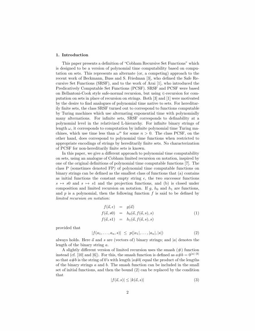
In this paper, we give a different approach to polynomial time computabilityon sets, using an analogue of Cobham limited recursion on notation, inspired byone of the original definitions of polynomial time computable functions [7]. Theclass P (sometimes denoted FP) of polynomial time computable functions onbinary strings can be defined as the smallest class of functions that (a) containsas initial functions the constant empty string ǫ, the two successor functionss 7→ s0 and s 7→ s1 and the projection functions, and (b) is closed undercomposition and limited recursion on notation. If g, h0 and h1 are functions,and p is a polynomial, then the following function f is said to be defined bylimited recursion on notation:

f(~a, ǫ) = g(~a)

f(~a, s0) = h0(~a, f(~a, s), s) (1)

f(~a, s1) = h1(~a, f(~a, s), s)

provided that|f(a1, . . . , an, s)| ≤ p(|a1|, . . . , |an|, |s|) (2)

always holds. Here ~a and s are (vectors of) binary strings; and |a| denotes thelength of the binary string a.

A slightly different version of limited recursion uses the smash (#) functioninstead (cf. [10] and [6]). For this, the smash function is defined as a#b = 0|a|·|b|

so that a#b is the string of 0’s with length |a#b| equal the product of the lengthsof the binary strings a and b. The smash function can be included in the smallset of initial functions, and then the bound (2) can be replaced by the conditionthat

|f(~a, s)| ≤ |k(~a, s)| (3)

2

where k is a function already known to be in P. In this version, f is said to bedefined by limited recursion on notation from g, h0, h1 and k.

Section 3 defines the Cobham Recursive Set Functions (CRSF) via an ana-logue of the definition of polynomial time functions with limited recursion.CRSF uses ∈-recursion instead of recursion on notation. In ∈-recursion, thevalue of f(x), for x a set, is defined in terms of the set of values f(y) for ally ∈ x. This means that the recursive computation of f(x) requires computingf(y) for all y in the transitive closure, tc(x), of x. The depth of the recur-sion is bounded by the rank, rank(x), of x. Of course, the cardinality of thetransitive closure of x, |tc(x)|, can be substantially larger than the cardinalityof the rank of x. The computational complexity of f(x) is thus bounded byboth the rank of x and by |tc(x)|; however, the bounds act in different ways.The intuition is that |tc(x)| polynomially bounds the overall work performed tocompute f(x), while rank(x) polynomially bounds the depth of the recursion inthe computation of f(x).

The definition of CRSF requires a set-theoretic analogue of the binary string# function. For this, Section 2 introduces a new set composition function, de-noted⊙, and a new set smash function, denoted #. The binary string function #allows defining functions of polynomial growth rate. The set smash function #is used to bound the sizes of sets introduced by ∈-recursion. The set function #,which can be viewed as a structured crossproduct, thus plays a similar role tothe binary string # function. However, the set smash function has to do doubleduty by providing polynomial bounds on both the ranks of sets and the car-dinalities of the transitive closures of sets. Namely, if z = x#y, then (a) therank of z is polynomially bounded by the ranks of x and y and (b) |tc(z)| ispolynomially bounded by |tc(x)| and |tc(y)|. The set function smash does morethan just bound the ranks and cardinalities; it also bounds the internal struc-ture of sets. For this reason, the bounding condition (3) needs to be replacedby a more complicated condition called 4-embeddability. Section 2 defines “τ4-embeds x into y”, denoted τ : x 4 y, in a way that faithfully captures thenotion that x is structurally “no more complex” than y. For technical reasons,the function τ is a one-to-many mapping. The condition “τ : f(~a, s) 4 k(~a, s)”is then the analogue of (3) which works for Cobham recursion on sets.

The outline of the paper is as follows. Section 2 defines the set compositionand smash functions; these are defined first using ∈-recursion and then in termsof Mostowski graphs. Section 3.1 defines various operations on set functions,and the class CRSF of Cobham Recursive Set Functions. Section 3.2 does sim-ple bootstrapping of CRSF, and shows the crossproduct and rank functions arein CRSF. Section 3.3 gives a normal form for CRSF functions by showing thata restricted class of “#-terms” can be used as the 4-bounds. As a corollary, itis shown that the growth rate of CRSF functions can be polynomially bounded.Sections 3.4 and 3.5 show that CRSF is closed under (unbounded) replacementand under course-of-values recursion. Section 3.6 proves that CRSF is closedunder an impredicative version of Cobham recursion, which has a relaxed em-bedding condition.

Section 4 takes up the question of how CRSF functions correspond to poly-

3

nomial time computability on binary strings. Following [11, 3, 1], we choose anatural method of encoding binary strings as hereditarily finite sets. We thenprove that, relative to these encodings, the CRSF functions are precisely theusual polynomial time computable functions. As mentioned earlier, similar re-sults were obtained by Arai for the PCSF functions. Sazonov [11] also defined aclass of polynomial time set functions. Sazonov’s polynomial time functions arethe same as CRSF functions when operating on hereditarily finite sets suitablyencoding binary strings, but are rather different for inputs which are generalsets. In particular, Sazonov’s functions when taking general hereditarily finitesets as inputs can be characterized as functions which operate in polynomialtime on the (finite) Mostowski graphs of the inputs. In contrast, our CRSFfunctions have recursion depth bounded by a polynomial of the rank of its in-puts. As a result, CRSF is a more restricted computational model of polynomialcomputation for general hereditarily finite sets. We feel it is natural and de-sirable that the computational power of CRSF depends on the ranks and thehereditary structure of its inputs.

Section 5 discusses a relationship between CRSF and PCSF. Instead of usingthe class PCSF identified by Arai, we work with a (conjecturally) larger classof functions which we call PCSF+. Theorems 35 and 36 and Corollary 37 statethat CRSF and PCSF+ have equivalent power over all sets (taking inputs asnormal inputs in the case of PCSF+).

The present paper is part of a cycle of three papers in preparation aboutCRSF functions. Another paper [4] discusses circuit computation models forset functions based on an alternative formulation of CRSF. A third paper [2]discusses set theoretic axioms and proof theory for CRSF.

Throughout the paper, we work in theory ZFC of Zermelo-Fraenkel set the-ory with choice. The axiom of choice is used only when we discuss cardinalities,and is not needed for anything else.

We thank the anonymous referee for feedback and corrections.

2. The set smash and lex smash functions

This section defines the “smash” function # for sets. We define a set compo-sition operation ⊙ and then the set smash function. We then present intuitiveconceptual definitions of these functions in terms of the Mostowski graphs ofsets.

Definition 1. The set composition function is the function a⊙b defined by∈-recursion as

∅⊙b = b

a⊙b = {x⊙b : x ∈ a}, for a 6= ∅.

We use rank(a) and tc(a) to denote the rank and the transitive closure of a.We write tc+(a) for tc(a) ∪ {a}, and rank+(a) for rank(a) + 1. As usual, |a|denotes the cardinality of a.

4

Lemma 2. The set composition function ⊙ satisfies the following:

1. a⊙∅ = a.

2. rank(a⊙b) = rank(b) + rank(a).

3. If a 6= a′, then a⊙b 6= a′⊙b.

4. tc(a⊙b) = tc(b) ∪ {a′⊙b : a′ ∈ tc(a)}.

5. |tc(a⊙b)| = |tc(a)|+ |tc(b)|.

6. ⊙ is associative: a⊙(b⊙c) = (a⊙b)⊙c.

Proof. Parts 1., 2., 4., and 6. are easily proved by ∈-induction on a. Part 3.is proved using extensionality and induction on the ranks of a and a′. Part 5.is an immediate consequence of parts 3. and 4. and the observation that b ∈tc+(a′⊙b), so the right hand side of part 4. is a disjoint union.

Definition 3. The set smash function is the function a#b defined by ∈-recursionon a as

a#b = b⊙{x#b : x ∈ a}. (4)

Lemma 4. The set smash function # satisfies the following:

1. ∅#b = b

2. a#∅ = a

3. rank(a#b) + 1 = (rank(b) + 1)(rank(a) + 1). Equivalently, rank+(a#b) =rank+(b) · rank+(a).

4. |tc(a#b)| + 1 = (|tc(a)| + 1)(|tc(b)| + 1). Equivalently, |tc+(a#b)| =|tc+(a)| · |tc+(b)|.

5. # is associative.

Proof. Part 1. is immediate from the definitions. Parts 2. and 3. are readilyproved by ∈-induction on a. We postpone the proof of part 4. until after dis-cussing the Mostowski graph next. For part 5. we can first prove the followingkind of distributive law by ∈-induction on a:

(a⊙b)#c = (a#c)⊙{y#c : y ∈ b}.

Using this one easily proves a#(b#c) = (a#b)#c by ∈-induction on a.

Observe that we do not have a general distributive law of the form

(a⊙b)#c = (a#c)⊙(b#c),

as rank((1⊙1)#1) = 5 but rank((1#1)⊙(1#1)) = 6.An intuitive understanding of the ⊙ and # functions can be obtained by

considering the Mostowski graph of a set.

5

Definition 5. Let A be a set. The Mostowski graph of A is the directed graphwith vertex set V = tc+(A), and edge relation E defined by 〈v1, v2〉 ∈ E iffv1 ∈ v2. More generally, any directed graph isomorphic to the Mostowski graphof A is called a Mostowski graph of A.

The Mostowski graph of A is well-founded (i.e., any subset of V has an E-minimal element) and is extensional (i.e., any distinct v1, v2 in V have differentsets of E-predecessors). Furthermore, a Mostowski graph must be “accessiblepointed”: (V,E) is accessible pointed provided there is a v ∈ V such that for allv′ ∈ V , v′E∗v holds, where E∗ is the reflexive, transitive closure of E. This vis the unique sink node of (V,E); in fact, v corresponds to the vertex A. Con-versely, it is an elementary fact that any well-founded, extensional, accessiblepointed, directed graph is a Mostowski graph for a unique set.

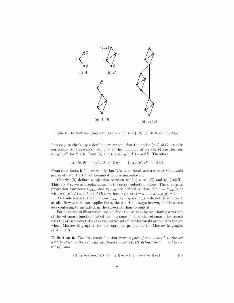
As usual, the integers are coded as von Neumann integers, so 0 = ∅, 1 = {0},2 = {0, 1}, etc. The Mostowski graphs of A = 2 and B = {1, 2} are shown inFigure 1.

We now define ⊙ and # in terms of Mostowski graphs. First, note thatextensionality and wellfoundedness imply that a Mostowski graph has a uniquesource node, and that accessible pointedness and wellfoundedness imply that ithas a unique sink node. Let GA = (VA, EA) and GB = (VB , EB) be Mostowskigraphs for the sets A and B. Then, assuming VA ∩ VB = ∅, the Mostowskigraph (V,E) for A⊙B can be obtained by identifying the sink vertex of GB andthe source vertex of GA. In other words, the sink node of B is replaced by acopy of GA; equivalently, the source node of A is replaced by a copy of GB. (SeeFigure 1.)

More formally, a Mostowski graph for A⊙B can be defined letting the nodesbe V := {〈1, a〉 : a ∈ tc+(A)} ∪ {〈0, b〉 : b ∈ tc(B)}, and letting the edges be thefollowing:

• 〈〈0, b′〉, 〈0, b〉〉 for all b′ ∈ b ∈ tc(B),

• 〈〈0, b〉, 〈1, ∅〉〉 for all b ∈ B, and

• 〈〈1, a′〉, 〈1, a〉〉 for all a′ ∈ a ∈ tc+(A).

Note that the nodes 〈0, b〉 correspond to the sets b, and the nodes 〈1, a〉 corre-spond to the sets a⊙B.

The Mostowski graph of A#B is obtained by replacing every vertex of GA

with a copy of the graph GB. This is pictured in Figure 1. Formally, we candefine a Mostowski graph G = (V,E) for A#B by letting the graph have vertexset V = {〈a, b〉 : a ∈ tc+(A), b ∈ tc+(B)}, and letting the edge set E contain:

• 〈〈a, b′〉, 〈a, b〉〉 for b′ ∈ b ∈ tc+(B) and

• 〈〈a′, B〉, 〈a, ∅〉 for a′ ∈ a ∈ tc+(A).

The intent is that 〈a, b〉 corresponds to the set

σA,B(a, b) := b⊙{a′#B : a′ ∈ a}. (5)

6

∅

1

2

(a) A

∅

1

2

{1, 2}

(b) B

(d) A#B(c) A⊙B

Figure 1: The Mostowski graphs for (a) A = 2, (b) B = {1, 2}, (c) A⊙B, and (d) A#B.

It is easy to check, by a double ∈-recursion, that the nodes 〈a, b〉 of G actuallycorrespond to these sets: For b 6= ∅, the members of σA,B(a, b) are the setsσA,B(a, b

′) for b′ ∈ b. From (4) and (5), σA,B(a,B) = a#B. Therefore,

σA,B(a, ∅) = {a′#B : a′ ∈ a} = {σA,B(a′, B) : a′ ∈ a}.

From these facts, it follows readily thatG is extensional, and a correct Mostowskigraph of a#b. Part 4. of Lemma 4 follows immediately.

Clearly, (5) defines a bijection between tc+(A) × tc+(B) and tc+(A#B).This lets # serve as a replacement for the crossproduct functions. The analogousprojection functions π1,A,B and π2,A,B are defined so that, for u = σA,B(a, b)with a ∈ tc+(A) and b ∈ tc+(B), we have π1,A,B(u) = a and π2,A,B(u) = b.

As a side remark, the functions σA,B, π1,A,B and π2,A,B do not depend on Aat all. However, in our applications, the set A is always known, and it seemsless confusing to include A in the subscript than to omit it.

For purposes of illustration, we conclude this section by mentioning a variantof the set smash function, called the “lex smash”. Like the set smash, lex smashuses the crossproduct A×B as the vertex set of its Mostowski graph; it is the setwhose Mostowski graph is the lexicographic product of the Mostowski graphsof A and B.

Definition 6. The lex smash function maps a pair of sets a and b to the seta#lexb which is the set with Mostowski graph (V,E) defined by V = tc+(a) ×tc+(b), and

E(〈a1, b1〉, 〈a2, b2〉) ⇔ a1 ∈ a2 ∨ (a1 = a2 ∧ b1 ∈ b2). (6)

7

The lex smash a#lexb has structure similar to a#b but with more edges inits Mostowski graph. We expect that using #lex instead of # would give us thesame class of functions CRSF, but we prefer # because it has a simple recursivedefinition.

Theorem 7. If (6) holds, so 〈a1, b1〉 precedes 〈a2, b2〉, then σA,B(a1, b1) ∈tc(σ(a2, b2)).

The proof of Theorem 7 is obvious from the Mostowski graph representationof A#B.

3. Cobham recursive set functions

This section defines the Cobham recursive set functions (CRSF) and provesa variety of closure properties.

3.1. Definition of CRSF

CRSF will be defined as an algebra of functions which take sets as inputsand produce sets as outputs. The following are the initial functions for CRSF.

(Projection) For 1 ≤ j ≤ n,

πnj (a1, . . . , an) = aj

(Pair)pair(a, b) = {a, b}

(Null)null( ) = ∅

(Union)

union(a) =⋃

a

(Conditional∈)

cond∈(a, b, c, d) =

{

a if c ∈ db otherwise.

CRSF also enjoys a variety of closure properties. Some of these hold bydefinition, and others will be derived.

(Separation) If g is an n-ary function, n ≥ 1, then (Separation) gives then-ary function f :

f(~a, c) = {b ∈ c : g(~a, b) 6= ∅}.

(Composition) If g is an n-ary function and ~h is a vector of n many m-aryfunctions, then (Composition) gives the m-ary function f :

f(~a) = g(~h(~a)).

8

(Replacement) If g is an (n+1)-ary function with n ≥ 1, then (Replace-ment) gives the n-ary function f :

f(~a, c) = {g(~a, b, c) : b ∈ c}.

(Bounded Replacement) If g is an (n+1)-ary function with n ≥ 1 and h isan n-ary function, then (Bounded Replacement) gives the n-ary function f :

f(~a, c) = {g(~a, b, c) : b ∈ c} ∩ h(~a, c).

(Cobham Recursion⊆) If n ≥ 1, g is an (n+1)-ary function and h is an n-aryfunction, then (Cobham Recursion⊆) gives the n-ary function f :

f(~a, c) = g(~a, c, {f(~a, b) : b ∈ c}) ∩ h(~a, c).

Note that the function h serves as a size bound for the values of f . This sizebound is rather crude however, since it requires f(x, ~y) to be a subset of h(x, ~y).Definition 9 gives a more general notion of size bound by requiring only that(the transitive closure of) f(x, ~y) be “embedded” into (the transitive closureof) h(x, ~y). We first define a simplified notion of “single-valued” embedding.

Definition 8. A set A is single-valued 4-embeddable in a set B if the followingholds: There is an injective function τ : tc(A) → tc(B) such that for all x ∈y ∈ tc(A), we have τ(x) ∈ tc(τ(y)). We call τ a single-valued embedding of Ainto B.

The idea for embeddings is that tc(A) and tc(B) are identified with theMostowski graphs of A and B. The relation “τ(x) ∈ tc(τ(y))” means that τ(x)precedes τ(y) in the sense that there is a non-trivial path in the Mostowskigraph from τ(x) to τ(y). The function τ shows that a copy of A is containedinside B, so A is structurally “no more complex” than B.

The actual definition of embedding uses multi-valued embeddings; namelyτ(x) will be a subset of tc(B), and in effect, is mapping x to each memberof τ(x). Let P(· · · ) denote the power set.

Definition 9. A set A is 4-embeddable in a set B, denoted A 4 B, if thefollowing holds: There is a function τ : tc(A) → P(tc(B)) such that for all x,τ(x) 6= ∅ and for all x 6= y, τ(x)∩ τ(y) = ∅, and such that for all x ∈ y in tc(A)and every u ∈ τ(y), there is some v ∈ τ(x) ∩ tc(u). We call τ an embeddingof A into B, and write τ : A 4 B. The condition τ(x) ∩ τ(y) = ∅ for x 6= y iscalled the injectivity condition.

As we shall see, A 4 B is a more general way to capture the intuition thatA is structurally “no more complex” than B. A single-valued embedding τ caneasily be converted into a (multi-valued) embedding, namely via x 7→ {τ(x)}.The multi-valued embedding x 7→ {x} is called the identity embedding.

The next proposition gives bounds on the rank of A and the cardinalityof tc(A). The proof is simple and left to the reader.

9

Proposition 10. Suppose A 4 B. Then rank(A) ≤ rank(B) and |tc(A)| ≤|tc(B)|.

An example of an embedding is given by Theorem 7: The map that sends(the set corresponding to) 〈x, y〉 to σA,B(x, y) is a single-valued 4-embeddingof A#lexB into A#B.

(Cobham Recursion4) If n ≥ 1, g is an (n+1)-ary function, h is an n-aryfunction and τ is an (n+1)-ary function, then (Cobham Recursion4) givesthe n-ary function f :

f(~a, c) = g(~a, c, {f(~a, b) : b ∈ c}),

provided that, for all ~a, c, we have τ(x,~a, c) : f(~a, c) 4 h(~a, c).The last condition means that the function x 7→ τ(x,~a, c) is an embedding

f(~a, c) 4 h(~a, c). Later, in Section 3.6, we will use a more general, impredicativenotion of embedding which allows f(~a, c) to also be an input to τ .

There is also an embedded version of replacement:

(Embedded Replacement) If n ≥ 1, g is an (n+1)-ary function, h is an n-aryfunction, and τ is an (n+1)-ary function, then (Embedded Replacement)gives the n-ary function f :

f(~a, c) = {g(~a, b, c) : b ∈ c}

provided that, for all ~a, c, we have τ(x,~a, c) : f(~a, c) 4 h(~a, c).

Cobham recursion can also be defined using a course-of-values (“CofV”) re-cursion. If f(~a, c) is a function, let f↾c(~a,−) denote the set of ordered pairs〈c′, f(~a, c′)〉 such that c′ ∈ c. As usual, an ordered pair 〈x, y〉 is equal to{{x}, {x, y}}.

(Cobham RecursionCofV4 ) If n ≥ 1, g is an (n+1)-ary function, h is an n-ary

function and τ is an (n+1)-ary function, then (Cobham RecursionCofV4 ) gives

the n-ary function f :

f(~a, c) = g(~a, c, f↾tc(c)(~a,−)), (7)

provided that, for all ~a, c, we have τ(x,~a, c) : f(~a, c) 4 h(~a, c).

Definition 11. Recall that integers are represented by the von Neumann inte-gers. The characteristic function χR of a relation R is defined by χR(~a) = 1 ifR(~a) and χR(~a) = 0 if ¬R(~a).

We now give the formal definition of CRSF:

10

Definition 12. The Cobham Recursive Set Functions, CRSF, are the functionsthat are obtained by starting with the initial functions (Projection), (Pair),(Null), (Union), (Conditional∈), and the set smash function #, and takingthe closure under (Composition), and (Cobham Recursion4). A relationR(~a) is in CRSF iff its characteristic function χR(~a) is in CRSF.

The next theorem shows that CRSF is also closed under (Bounded Re-placement) and (Embedded Replacement), as well as ∆0-separation. It fol-lows that CRSF contains all the rudimentary relations [8]. Theorems 23 and 29will later show closure under (Replacement) and (Cobham RecursionCofV

4 ).Theorem 30 will prove closure under impredicative versions of Cobham recur-sion.

3.2. Simple closure properties for CRSF

Theorem 13 establishes some basic properties of CRSF. After that, thecrossproduct and rank functions are shown to be in CRSF; however, the prooffor crossproduct will be finished only after CRSF is shown to be closed under(Replacement).

It is useful to note that parts 1.-11. of Theorem 13 do not require the useof smash, and part 1. does not use recursion. Furthermore, its proof requiresonly single-valued embeddings. (Subsequent to Theorem 13 we will need almostexclusively to consider multi-valued embeddings.)

Theorem 13. The following hold for CRSF.

1. CRSF contains the functions a 7→ {a} and

cond=(a, b, c, d) =

{

a if c = db otherwise.

2. CRSF is closed under (Embedded Replacement).

3. CRSF is closed under (Separation).

4. CRSF contains the binary functions a \ b and a ∩ b.

5. CRSF is closed under (Cobham Recursion⊆).

6. CRSF is closed under (Bounded Replacement).

7. The CRSF relations are closed under Boolean operations.

8. The CRSF relations are closed under bounded (∆0) quantification.

9. The function a 7→⋂

a is in CRSF. By convention⋂

∅ = ∅.

10. The function a 7→ tc(a) is in CRSF.

11. The function a, b 7→ 〈a, b〉 := {{a}, {a, b}} is in CRSF. In addition, CRSFcontains projection functions satisfying π1(〈a, b〉) = a and π2(〈a, b〉) = b,and contains the relation ispair(x) that tests whether x is an ordered pair〈a, b〉.

11

12. The binary functions ⊙ and ⊙−1 are in CRSF, where

a⊙−1b =

{

z such that a = z⊙b∅ if no such z exists.

13. The three functions a, b, a′, b′ 7→ σa,b(a′, b′) and a, b, x 7→ π1,a,b(x) and

a, b, x 7→ π2,a,b(x) are in CRSF.

Proof. 1. As usual, {a} = {a, a}. Then cond= is defined as cond∈(a, b, c, {d}).2. To define f from g, h and τ as in (Embedded Replacement), first

define k by

k(~a, b, c) =

g(~a, b, c) if b ∈ c{k(~a, d, c) : d ∈ c} if b = c∅ otherwise

with the aid of cond= and cond∈, and using (Cobham Recursion4) with thebounding function h′(~a, b, c) = h(~a, c) and the embedding function τ ′(x,~a, b, c) =τ(x,~a, c). Then f(~a, c) = k(~a, c, c).

3. To define f from g as in (Separation), first define k(~a, b, c), again withthe aid of cond= and cond∈, as

k(~a, b, c) =

{

{b} if b ∈ c and g(~a, b) 6= 0∅ otherwise.

Then define f(~a, c) =⋃

{k(~a, b, c) : b ∈ c} by (Embedded Replacement)using the bounding function h(~a, b, c) = c, and the single-valued embeddingfunction τ(x,~a, b, c) = x.

4. The set difference function can be defined using (Separation) by

a \ b = {x ∈ a : cond∈(∅, 1, x, b) 6= ∅}.

Intersection is defined by a ∩ b = ((a ∪ b) \ (a \ b)) \ (b \ a).5. The fact that (Cobham Recursion⊆) can be simulated by (Cobham

Recursion4) is immediate from the facts that binary intersection (∩) is inCRSF and that a ⊆ b implies a 4 b using the identity function as a single-valued embedding.

6. Suppose f is defined from g and h as in (Bounded Replacement).Then define

g′(~a, b, c) =

{

g(~a, b, c) if g(~a, b, c) ∈ h(~a, c)h(~a, c) otherwise.

Define f ′(~a, c) = {g′(~a, b, c) : b ∈ c} by (Embedded Replacement) usingthe bounding function h′(~a, c) = {h(~a, c)} = 1⊙h(~a, c) and the single-valuedembedding function τ(x,~a, b, c) = x. Finally, f(~a, c) = f ′(~a, c) \ {h(~a, c)}, sof ∈ CRSF.

7. Define the function f¬ and f∨ by

f¬(a) = 1 \ a and f∨(a, b) = a ∪ b.

12

These functions implement negation and disjunction, and therefore, by compo-sition, the CRSF relations are closed under Boolean operations.

8. To show closure under ∆0 quantification, it now suffices to prove that ifR is a CRSF relation, then so is S(~a, c) ⇔ ∃b∈cR(~a, b). For this, define

χS(~a, c) =⋃

{χR(~a, b) : b ∈ c}.

This is a valid use of (Bounded Replacement) and (Union) since χS(a,~c) ⊆ 1.9.

⋂

a can be defined as {x ∈⋃

a : ∀y∈a (x ∈ y)}.10. The transitive closure tc(a) can be defined using (Cobham Recursion4)

astc(a) = a ∪

⋃

{tc(x) : x ∈ a}

with the bounding function h(a) = a since tc(a) 4 a using the identity functionas the single-valued embedding.

11. The ordered pair function 〈a, b〉 is in CRSF as it is defined with threeuses of pair. To define the projection functions note that, for all a, b,

{a, b} =⋃

〈a, b〉,

a =⋃

{z ∈ {a, b} : {z} ∈ 〈a, b〉},

b =

{

a if 〈a, b〉 = 〈a, a〉⋃

({a, b} \ {a}) otherwise.

These facts immediately allow π1 and π2 to be expressed as CRSF functions.Finally,

ispair(z) = cond=(1, ∅, z, 〈π1(z), π2(z)〉).

12. The function a⊙b is defined as in Definition 1 by (Cobham Recursion4)by letting

a⊙b =

{

b if a = ∅{a′⊙b : a′ ∈ a} otherwise.

For the bounding function, let h(a, b) = a#b.6 The single-valued embeddingfunction τ can be defined as

τ(x, a, b) =

{

x if x ∈ tc+(b)x#b otherwise.

To define ⊙−1, observe that there is a z such that a = z⊙b exactly when

b ∈ tc+(a) ∧ (∀c ∈ tc+(a))(c ∈ tc+(b) ∨ (∀d ∈ c)(b ∈ tc+(d))). (8)

So ⊙−1 is defined by (Cobham Recursion4) as

a⊙−1b =

{

{a′⊙−1b : a′ ∈ a} if a 6= b and (8) holds∅ otherwise.

6It is overkill to use the # function to bound the ⊙ function. The alternative would be toinclude ⊙ in the base functions in the definition of CRSF.

13

For the single-valued embedding, let h(a, b) = a⊙b and τ(x, a, b) = x⊙b.13. The function a, b 7→ {a′#b : a′ ∈ a} is defined by (Bounded Replace-

ment), since a′#b ∈ tc(a#b) for a′ ∈ a. Therefore, (5) gives a CRSF definitionof σa,b(a

′, b′).The function π1,a,b can be defined using (Separation) and (Union) as7

π1,a,b(u) =⋃

{a′ ∈ tc+(a) : ∃b′ ∈ tc+(b) s.t.u = σa,b(a′, b′)}.

Note that the union is taken over a set of size at most one. The function π2,a,b

is defined similarly.

The next theorem states that crossproduct is a CRSF function; for this, #is needed. This is not surprising as # is itself a kind of crossproduct; however,the proof is somewhat difficult and will be completed in Section 3.4.

Theorem 14. The crossproduct function a× b is in CRSF.

The proof of Theorem 14 defines crossproduct as

a× b =⋃

{{a′} × b : a′ ∈ a},

where{z} × b := {〈z, b′〉 : b′ ∈ b},

and uses two applications of (Replacement) and (Union). However, theclosure of CRSF under (Replacement) will not be proved until Theorem 23.We thus postpone completing the proof of Theorem 14 pending the proof ofTheorem 23.

We now prove that the rank function is in CRSF. The proof uses (Cob-ham Recursion4), but establishing the embedding condition is unexpectedlydifficult and uses a multi-valued embedding. We do not know any way to use asingle-valued embedding instead.

Theorem 15. The function a 7→ rank(a) is in CRSF.

Proof. Since rank(a) =⋃

rank+(a), it suffices to show rank+ is in CRSF. Thelatter can be defined using (Cobham Recursion4) since

rank+(a) = Succ(⋃

{rank+(x) : x ∈ a}), (9)

where Succ(S) = S ∪ {S}. For the bounding function, take h(a) = {a}. Wedefine the (multi-valued) embedding τ by letting τ(α) equal the members oftc+(a) of rank α. This τ is defined with the aid of a function RksLE(a, b) (for“ranks less than or equal to”) which is equal to the set of a′ ∈ tc+(a) which

7Here we take advantage of the fact that a is available, but with a little more work it ispossible to define π1,a,b(u) without using a.

14

have rank ≤ rank(b). RksLE is defined using (Cobham Recursion⊆) and(Separation) by

RksLE(a, b) ={

a′ ∈ tc+(a) : a′ ⊆⋃

{RksLE(a, b′) : b′ ∈ b}}

.

We have rank(a) ≤ rank(b) iff a ∈ RksLE(a, b). Then τ is defined using (Sep-aration) as

τ(x, a) = {a′ ∈ tc+(a) : x ∈ RksLE(x, a′) ∧ a′ ∈ RksLE(a′, x)}.

3.3. #-terms as bounding functions

The section states and proves a crucial technical result which states thatCRSF functions can be embedded into sets constructed from terms, called “#-terms”, involving ⊙ and #. Corollary 22 shows that this immediately impliespolynomial bounds on the growth rates of CRSF functions. This is also the keytool needed in Section 3.4 for the proof that CRSF is closed under (Replace-ment).

Definition 16. A #-term is a term built up from variables, the constant sym-bol 1, and the function symbols ⊙ and #.

Any #-term t(a1, . . . , ak) represents a CRSF function. The next theoremshows that CRSF functions have bounded growth rate in the sense that theirvalues are embeddable in a #-term.

Theorem 17. Let f(a1, . . . , ak) be in CRSF. There is a #-term t(a1, . . . , ak)and a CRSF function τ(x, a1, . . . , ak) such that τ : f(a1, . . . , ak) 4 t(a1, . . . , ak).

For the embedding τ of Theorem 17, the inputs ai serve as parameters, or“side variables”: it is the mapping x 7→ τ(x,~a) that satisfies the properties ofDefinition 9. Before proving Theorem 17, we establish some simple lemmasshowing how #-terms act like monotone functions w.r.t. embeddings.

Lemma 18. 4 is transitive: If A 4 B and B 4 C, then A 4 C. Furthermore,if τ1 : A 4 B and τ2 : B 4 C are valid, where A, B, C, τ1 and τ2 are given byCRSF functions, then there is a CRSF function τ such that τ : A 4 C is valid.

The hypothesis of the second half of Lemma 18 means that there are param-eters ~a so that A = A(~a), B = B(~a) and C = C(~a) are functions of ~a, and theembeddings τi depend on the parameters and have the forms x 7→ τi(x,~a). Inthis, case, the function x 7→ τ(x,~a) gives an embedding τ : A(~a) 4 C(~a).

Proof. Let τ1 : A 4 B and τ2 : B 4 C. Thus, τ1 : tc(A) → P(tc(B)) andτ2 : tc(B) → P(tc(C)). Define τ : tc(A) → P(tc(C)) by letting

τ(x) =⋃

{τ2(z) : z ∈ τ1(x)}. (10)

We claim τ : A 4 C. It is clear that if x 6= y, then τ(x) ∩ τ(y) = ∅. Supposex ∈ y ∈ tc(A) and u ∈ τ(y). We have u ∈ τ2(z) for some z ∈ τ1(y). Since τ1

15

is a 4-embedding, there is a w ∈ τ1(x) ∩ tc(z). By the definition of transitiveclosure, there is a finite sequence w0=w,w1, . . . , wℓ=z such that wi ∈ wi+1 forall i. Since τ2 is also a 4-embedding, there are v0, . . . , vℓ=u such that eachvi ∈ τ2(wi)∩ tc(vi+1). Thus v = v0 is in τ2(w)∩ tc(u) and hence in τ(x)∩ tc(u).

Since τ(x) ⊆ tc(C), τ is defined by (Bounded Replacement) and (Union),or alternately by (Separation). Thus by Theorem 13, τ is in CRSF if A, B,C, τ1 and τ2 are.

Lemma 19. If A 4 B and C 4 D, then A⊙C 4 B⊙D and A#C 4 B#D.Furthermore, if τ1 : A 4 B and τ2 : C 4 D are valid, for A, B, C, D, τ1 and τ2given by CRSF functions, then there are CRSF functions τ and τ ′ such thatτ : A⊙C 4 B⊙D and τ ′ : A#C 4 B#D are valid.

Proof. Let τ1 : A 4 B and τ2 : C 4 D. Define τ : tc(A⊙C) → P(tc(B⊙D))by setting τ(x) = τ2(x) for x ∈ tc(C), and setting τ(x⊙C) = τ1(x)⊙D forx ∈ tc(A). More formally,

τ(x) =

{

τ2(x) if x ∈ tc(C){y⊙D : y ∈ τ1(x⊙−1C)} otherwise.

(11)

Since τ(x) ⊆ tc(B⊙D), closure under (Separation) implies that if A, B, C,D, τ1 and τ2 are given by CRSF functions, then so is τ .

We claim that τ : A⊙C 4 B⊙D. The fact that τ(x) and τ(y) are disjointfor x 6= y follows from the properties of τ1 and τ2 and part 3. of Lemma 2.So, suppose x ∈ y ∈ tc(A⊙C) and u ∈ τ(y). We need to prove there is av ∈ τ(x) ∩ tc(u). There are three cases to consider. The first case is wherex ∈ y ∈ tc(C): there must be a v ∈ τ2(x)∩ tc(u), and this v works for τ as well.The second case is when x = x′⊙C and y = y′⊙C for some x′ ∈ y′ ∈ tc(A). Wealso have u = u′⊙D and u′ ∈ τ1(y

′); thus there is a v′ ∈ τ1(x′) ∩ tc(u′). Then

v = v′⊙D ∈ τ(x) ∩ tc(u). The third case is where x ∈ C and y = C. Then,τ(x) ⊆ tc(D), and τ(y) = τ1(∅)⊙D. Any u ∈ τ(y) has the form u = u′⊙D, andsince τ(x) and τ1(∅) are both non-empty, the desired v exists. Thus τ : A⊙C 4

B⊙D.For the second assertion, we now define τ ′ : tc(A#C) → P(tc(B#D)).

For x ∈ tc(A#C), set y = π1,A,C(x) and z = π2,A,C(x) so that y ∈ tc+(A),z ∈ tc+(C), and x = σA,C(y, z) = z⊙{y′#C : y′ ∈ y}, and define

τ ′(x) = {σB,D(y′, z′) : y′ ∈ τ+1 (y) and z′ ∈ τ+2 (z)}, (12)

where τ+2 is the same as τ2 except extended to map C to {D}. It is easy toverify that if A, B, C, D, τ1 and τ2 are given by CRSF functions, then so is τ ′.

The proof that τ ′ : A#C 4 B#D is similar in spirit to the above argumentand is left for the reader.

Lemma 20. Suppose τi : Ai 4 Bi is valid for i = 1, . . . , n, where Ai, Bi and τiare given by CRSF functions. Let t(x1, . . . , xn) be a #-term. Then there is a

CRSF function τ so that τ : t( ~A) 4 t( ~B) is valid.

16

Proof. This follows readily from Lemmas 18 and 19, and induction on the com-plexity of t.

Proof of Theorem 17. We use induction based on the definition of CRSF func-tions. For the projection function πn

j , it is trivial; just take the bounding termt(a1, . . . , an) = aj and let the single-valued embedding function τ be the identityfunction. For cond∈, use t(a, b, c, d) = a⊙b and define a single-valued embed-ding τ by letting τ(x) equal x for x ∈ tc(b) and equal x⊙b for x ∈ tc(a) \ tc(b).For pair(a, b), let t(a, b) = 1⊙a⊙1⊙b and define a single-valued embedding τ(x)to equal x for x ∈ tc+(b) and to equal x⊙1⊙b for x ∈ tc+(a)\tc+(b). For union,the identity function is a single-valued embedding of

⋃

a into a. Of course, theset smash function a#b is single-valued 4-embedded into itself by the identityfunction.

Suppose f(~a) is defined by (Composition) from g(u1, . . . , un) and hi(~a)for i = 1, . . . , n. By the induction hypothesis, there are #-terms s and ti andCRSF functions τ(x, ~u) and τi(x,~a) so that τ : g(~u) 4 s(~u) and τi : hi(~a) 4 ti(~a)

for i = 1, . . . , n. In particular, τ(x,~h(~a)) : g(~h(~a)) 4 s(~h(~a)). Lemma 20 gives

a CRSF-function σ(x,~a) so that σ : s(~h(~a)) 4 s(~t(~a)). Then Lemma 18 gives

ρ(x,~a) such that ρ : f(~a) = g(~h(~a)) 4 s(~t(~a)) as desired.Finally, if f is defined by (Cobham Recursion4), then τ : f(a,~c) 4 h(a,~c)

for some CRSF functions h and τ . The induction hypothesis gives a #-termt(a,~c) and a CRSF function τ ′ such that τ ′ : h(a,~c) 4 t(a,~c). Lemma 18immediately gives a CRSF function τ ′′ so that τ ′′ : f(a,~c) 4 t(a,~c).

The proof of Theorem 17 actually gives a stronger result. Examinationof its proof and the proofs of Lemmas 18 and 19 shows that the embeddingfunctions are created using only the closure properties of CRSF established inTheorem 13. Indeed, they are created from the functions ⊙, #, ⊙−1, π1,A,B,π2,A,B and functions already shown to be in CRSF using composition and The-orem 13. Furthermore, the proof of Theorem 13 shows that the same closureproperties still apply when only #-terms are allowed as bounding functions.This establishes:

Theorem 21. The class CRSF would be unchanged if the definition of (Cob-ham Recursion4) were changed to require the bounding function h(~a, c) to bea #-term.

Corollary 22. Let f(~a) be a CRSF function. Then there are polynomials p andq so that rank(f(~a)) ≤ p(maxi{rank(ai)}) and |tc(f(~a))| ≤ q(maxi{|tc(ai)|}).

The corollary follows immediately from Lemma 4, Proposition 10, and The-orem 17. Namely, #-terms have polynomially bounded increase in rank, andpolynomially bounded increase in cardinality of their transitive closure, andthese bounds are preserved by embeddings.

3.4. Closure of CRSF under replacement

We can now show closure under (unbounded) replacement.

17

Theorem 23. CRSF is closed under (Replacement).

Proof. Suppose g(~a, b, c) is in CRSF and f(~a, c) is defined from g by (Replace-ment) as f(~a, c) = {g(~a, b, c) : b ∈ c}. We must show f is also in CRSF. ByTheorem 17, there is a #-term tg(~a, b, c) and a CRSF function τg(x,~a, b, c) suchthat τg : g(~a, b, c) 4 tg(~a, b, c). Since f depends on ~a and c but not b, it is incon-venient to have tg and τg depend on b. Accordingly, we let t′g(~a, c) = tg(~a, c, c).By Lemmas 18-20, there is a CRSF function τ ′g(x,~a, b, c) so that for all ~a and cand all b ∈ tc(c), we have τ ′g : g(~a, b, c) 4 t′g(~a, c).

A slight modification of τ ′g gives a CRSF function τ ′′g : {g(~a, b, c)} 4 t′′g (~a, c),where t′′g(~a, c) is the #-term 1⊙t′g(~a, c)

Let t(~a, c) be the #-term c#t′g(~a, c). The intuition is that f(~a, c), which isthe set of g(~a, b, c)’s for b ∈ c, can be embedded into t(~a, c) by an embedding τthat sends (the transitive closure of) each {g(~a, b, c)} into the “b-th copy” oft′g(~a, c). Formally, we let T abbreviate t′g(~a, c), and define

τ(x,~a, c) = {z ∈ c#T : π1,c,T (z) ∈ c ∧ x ∈ tc+(g(~a, π1,c,T (z), c))

∧ π2,c,T (z) ∈ τ ′′g (x,~a, π1,c,T (z), c)}.

This is a definition by (Separation), and thus τ is a CRSF function. Tounderstand τ , note that τ(x,~a, c) is the set of values z = σc,T (b, u) for thevalues of b and u such that b ∈ c, x ∈ tc+({g(~a, b, c)}), and u ∈ τ ′′g (x,~a, b, c).From this, it is clear that τ : f(~a, c) 4 c#T = t(~a, c). This means that thedefinition of f(~a, c) is actually a definition by (Embedded Replacement), sof is in CRSF.

This also establishes Theorem 14 about forming crossproducts since, as dis-cussed earlier, it follows from the closure of CRSF under (Replacement).

3.5. Course-of-values encodings

The graph of a function f is the class of tuples 〈~a, b〉 such that f(~a) = b.When f = f(~a, c) has a distinguished input c, we will also define the “course-of-values function of f” to be the function f∗ such that f∗(~a, c) gives simulta-neously all tuples 〈c′, f(~a, c′)〉 such that c′ ∈ tc+(c). The conventional way toencode these tuples would be as a set of ordered pairs; e.g., to define f∗(~a, c)to be the same as f↾tc+(c)(~a, c). However, we shall use an alternate specializedencoding instead. Specifically, we define

f∗(~a, c) = {∅, 〈c, f(~a, c)〉}⊙{f∗(~a, c′) : c′ ∈ c}. (13)

The intuition is that the tuple 〈c, f(~a, c)〉 sits “on top of” the tuples 〈c′, f(~a, c′)〉for c′ ∈ tc(c). This will be helpful for defining 4-embeddings, as it can give theembedding function access to the values of f(~a, c′) for c′ ∈ tc(c).

We record some simple but useful properties of f∗(~a, c). First, we have thatf∗(~a, c) = {z, 〈c⊙z, f(~a, c)⊙z〉} where we write z for the set {f∗(~a, c′) : c′ ∈ c}.So f∗(~a, c) has exactly two elements, of different ranks; the lower rank elementis z and the higher rank element is an ordered pair. Second, f∗(~a, c) is not an

18

ordered pair. If z = ∅, this is direct. Otherwise, an ordered pair is either asingleton or has one element a subset of the other, and neither is possible here.Third, z is not an ordered pair, since an ordered pair must contain a singleton;and, by the above, z does not contain any ordered pairs.

We need a variety of utility CRSF functions to decode structures of theform (13).

Definition 24. We define

MnR′(F ) =⋃

{u ∈ F : ∀u′ ∈ F, rank(u) ≤ rank(u′)}MxR′(F ) =

⋃

{u ∈ F : ∀u′ ∈ F, rank(u) ≥ rank(u′)}MxR(u) = MxR′(u)⊙−1MnR′(u)MxR1(u) = π1(MxR(u))MxR2(u) = π2(MxR(u)).

Here “MnR” and “MxR” stand for “minimum/maximum rank”. If u ={∅, 〈c, v〉}⊙z, then MxR′(u) = 〈c, v〉⊙z and MnR′(u) = ∅⊙z = z. ThusMxR(u) = 〈c, v〉, MxR1(u) = c and MxR2(u) = v. In particular this givesMnR′(f∗(~a, c)) = {f∗(~a, c′) : c′ ∈ c}, MxR1(f

∗(~a, c)) = c and MxR2(f∗(~a, c)) =

f(~a, c). Hence

Proposition 25. If f∗ ∈ CRSF, then f ∈ CRSF.

Lemma 26. There is a CRSF function AllValues such that, for any function fand sets ~a, c we have AllValues(f∗(~a, c)) = f↾tc(c)(~a,−).

Proof. We define an auxiliary function Stars recursively by

Stars(F ) =

∅ if F is an ordered pair⋃

{Stars(F ′) : F ′ ∈ F} if F is not an ordered pair, butcontains an ordered pair

F ∪⋃

{Stars(F ′) : F ′ ∈ F} otherwise.

By the earlier remarks about the structure of f∗, writing z for the set {f∗(~a, c′) :c′ ∈ c} we have

Stars(f∗(~a, c)) = Stars({z, 〈c⊙z, f(~a, c)⊙z〉})

= Stars(z) ∪ Stars(〈c⊙z, f(~a, c)⊙z〉)

= Stars(z)

= {f∗(~a, c′) : c′ ∈ c} ∪⋃

c′∈c

Stars(f∗(~a, c′)).

Hence Stars(f∗(~a, c)) = {f∗(~a, c′) : c′ ∈ tc(c)}. Each value Stars(F ) is asubset of tc(F ), so this is an instance of (Cobham Recursion⊆) and thusStars is in CRSF. We define AllValues(F ) by (Replacement) as {MxR(u) :u ∈ Stars(F )}.

Finally, we introduce two predicates IsCofVTopg and IsCofVSetg to help usfind our place inside the internal structure of sets f∗(~a, c). These will be usedwhen constructing embeddings from such sets into smash terms.

19

Definition 27. Let f be defined by (possibly unbounded) course-of-values re-cursion from a function g so that

f(~a, c) = g(~a, c, f↾tc(c)(~a,−)).

IsCofVTopg(F,~a) expresses that F is a set of the form f∗(~a, c) for some c.IsCofVSetg(F,~a) expresses that F is a set of such sets.

Lemma 28. If g is in CRSF, then so are IsCofVTopg and IsCofVSetg.

Proof. Combining the recursive definitions of f∗ in terms of f and of f interms of g, we can write down a definition of IsCofVTopg and IsCofVSetg bysimultaneous recursion. We will do this slightly indirectly. Let IsCofVg be thefunction

IsCofVg(F,~a) =

∅ if IsCofVTopg(F,~a)1 if IsCofVSetg(F,~a)2 otherwise.

Since this has range {0, 1, 2}, we can write the simultaneous recursion as adefinition of IsCofVg by (Cobham Recursion⊆):

IsCofVg(F,~a) =

∅ if F = {∅, 〈MxR1(F ),MxR2(F )〉}⊙MnR′(F ),IsCofVg(MnR′(F ),~a) = 1,MxR1(F ) = {MxR1(F

′) : F ′ ∈ MnR′(F )} andMxR2(F ) = g(~a,MxR1(F ),AllValues(F ))

1 if {IsCofVg(F′,~a) : F ′ ∈ F} ⊆ {∅}

2 otherwise.

This is not quite an instance of (Cobham Recursion⊆) as written, but be-comes one if we replace the second line of the ∅ case with 1 ∈ {IsCofVg(F

′,~a) :F ′ ∈ F}. This is equivalent, since F consists of MnR′ and an ordered pair whichcannot satisfy IsCofVSetg. Hence IsCofVg is in CRSF, so the two predicatesare as well.

Theorem 29. CRSF is closed under (Cobham RecursionCofV4 ).

Proof. Suppose CRSF functions g and τ1 and a #-term h are used to define afunction f1 by (Cobham RecursionCofV

4 )

f1(~a, c) = g(~a, c, f1↾tc(c)(~a,−)),

where τ1(x,~a, c) : f1(~a, c) 4 h(~a, c). We want to show f1 ∈ CRSF. It willbe helpful to have c available as an extra side parameter, so we define a newfunction f by (Cobham RecursionCofV

4 ) as

f(~a, c, c′) =

{

g(~a, c′, f↾tc(c′)(~a, c,−)) if c′ ∈ tc+(c)∅ otherwise.

(14)

Since f1(~a, c) = f(~a, c, c), it suffices to prove that f(~a, c, c′) is in CRSF. Let-ting τ(x,~a, c, c′) = τ1(x,~a, c

′), we have τ(x,~a, c, c′) : f(~a, c, c′) 4 h(~a, c′). Wehenceforth implicitly assume that c′ ∈ tc+(c).

20

Let f∗ be the course-of-values function for f :

f∗(~a, c, c′) = {∅, 〈c′, f(~a, c, c′)〉}⊙{f∗(~a, c, c′′) : c′′ ∈ c′}. (15)

By Proposition 25, it suffices to show f∗ is in CRSF. We will use (CobhamRecursion4), by giving a recursive definition of f∗, a bounding term h∗(~a, c)and a CRSF embedding function τ∗(x,~a, c).8

For the recursive definition of f∗, observe that

f↾tc(c′)(~a, c,−) =⋃

c′′∈c′

f↾tc+(c′′)(~a, c,−)

=⋃

c′′∈c′

[{MxR(f∗(~a, c, c′′))} ∪ AllValues(f∗(~a, c, c′′))] .

So from {f∗(~a, c, c′′) : c′′ ∈ c′} we can construct f↾tc(c′)(~a, c,−), then use g toconstruct f(~a, c, c′), then use (15) to construct f∗(~a, c, c′), all in CRSF.

The main difficulty in defining the embedding τ∗ is that it has to analyzethe meaning of its input x. Here x comes from the course-of-values, but willnot in general be a course-of-values set itself, but rather will be a memberof tc(f∗(~a, c, c′)). By construction, for every such x there is c′′ ∈ tc(c′) andy ∈ tc+({∅, 〈c′′, f(~a, c, c′′)〉}) such that

x = y⊙{f∗(~a, c, c′′′) : c′′′ ∈ c′′}. (16)

Define

TopCofVSetg(x,~a) =⋃

{F ∈ tc+(x) : IsCofVSetg(F,~a)∧

¬(∃F ′∈tc+(x))(F ∈ tc(F ′) ∧ IsCofVSetg(F′,~a))}.

We claim that TopCofVSetg(x,~a) = {f∗(~a, c, c′′′) : c′′′ ∈ c′′}. To see this,let G = {f∗(~a, c, c′′′) : c′′′ ∈ c′′} and suppose there is an F = y′⊙G 6= Gsatisfying IsCofVSetg(F,~a) with y′ ∈ tc(y). Take F and y′ to be of minimalrank satisfying these conditions. We have y′ 6= ∅; furthermore, any y′′ ∈ y′

satisfies IsCofVTopg(y′′⊙G). Thus y′′ 6= ∅, and y′′′ = MnR(y′′) ∈ y′′ satisfies

IsCofVSetg(y′′′⊙G). By the minimality of y′, we have y′′′⊙G = G. It follows

that y′′ = {∅, 〈c′′, f(~a, c, c′′)〉}. This contradicts y′′ ∈ tc(y) and the choice of y.Therefore, we can recover c′′ from x by

cValueg(x,~a) = {MxR1(F ) : F ∈ TopCofVSetg(x,~a)}.

We are now ready to define τ∗ and h∗. By Lemma 20, from τ we canconstruct a CRSF function τ ′ such that τ ′(x,~a, c, c′′) : f(~a, c, c′′) 4 h(~a, c), aslong as c′′ ∈ tc+(c) since in this case c′′ 4 c by the identity embedding. From

8It would be permitted to have c′ be a parameter to τ∗ and h∗, but we do not need it.

21

this, it follows readily that there is a #-term s(~a, c) and a CRSF function τ ′′

such thatτ ′′(x,~a, c, c′′) : {{∅, 〈c′′, f(~a, c, c′′)〉}} 4 s(~a, c) (17)

whenever c′′ ∈ tc+(c). Let h∗(~a, c) equal c#s(~a, c). Finally define τ∗(x,~a, c) toequal

{σc,s(~a,c)(c′′, u) : u ∈ τ ′′(x⊙−1TopCofVSetg(x,~a),~a, c, c

′′)}

where c′′ = cValue(x,~a).It is straightforward to verify that τ∗ is a CRSF function and is a (multi-

valued) embedding f∗(~a, c) 4 h∗(~a, c). The intuition is that c′′ is such that xis in the “{∅, 〈c′′, f(~a, c, c′′)〉}” part of the course-of-values set, and then τ∗ iscomputed taking the values given by τ ′′ and mapping them to the c′′-th copyof s(~a, c) in c#s(~a, c). In particular, suppose that x2 ∈ x1 ∈ tc(f∗(~a, c, c′))and let c′′ = cValue(x1,~a) and let c′′′ = cValue(x2,~a). If c′′ = c′′′ thenTopCofVSetg(x1,~a) = TopCofVSetg(x2,~a) and for every u ∈ τ∗(x1,~a, c) thereis a v ∈ τ∗(x2,~a, c) ∩ tc(u) by the properties of τ ′′. The only other possibilityis that x1 = TopCofVSetg(x1,~a) and x2 = f∗(~a, c′′′) with c′′′ ∈ c′′. In this casethe embedding property follows from the properties of σc,s(~a,c).

This completes the proof that f∗ is in CRSF.

3.6. Impredicative embeddings

The section proves that CRSF is closed under Cobham recursion even when“impredicative” embeddings are used to bound functions. Recall that (Cob-ham Recursion4) and (Cobham RecursionCofV

4 ) were defined with the con-dition that for all ~a, c we have τ(x,~a, c) : f(~a, c) 4 h(~a, c). We form impredica-tive versions of these by allowing τ to have f(~a, c) as an additional input andrequiring instead that, for all ~a, c,

τ(x,~a, c, f(~a, c)) : f(~a, c) 4 h(~a, c). (18)

Like the earlier bounding condition, this impredicative bounding condition im-plies that f(~a, c) has rank bounded by rank(h(~a, c)) and has |tc(f(~a, c))| ≤|tc(h(~a, c))|. The difference is that with f(~a, c) as an additional parameter, itis potentially easier for τ to compute a 4-embedding. Nonetheless, the nexttheorem shows that this gives no additional power for defining CRSF functions.

Theorem 30. CRSF is closed under the impredicative versions of (CobhamRecursion4) and (Cobham RecursionCofV

4 ).

As a corollary, CRSF is also closed under the impredicative version of (Em-bedded Replacement), as the proof of part 2. of Theorem 13 still applies.

Proof. The proof uses the techniques of the proof of Theorem 29 from the pre-vious section. We prove only the (Cobham RecursionCofV

4 ) case. The case of(Cobham Recursion4) follows as a corollary, or alternatively can be proveddirectly by using the “RecValues” function introduced in Section 5.1 below inplace of the “AllValues” function.

22

Similarly to the proof of Theorem 29, assume f(~a, c, c′) is defined from theCRSF functions g and τ and a #-term h by

f(~a, c, c′) =

{

g(~a, c′, f↾tc(c′)(~a, c,−)) if c′ ∈ tc+(c)∅ otherwise

but now with only the impredicative embedding condition

τ(x,~a, c, c′, f(~a, c, c′)) : f(~a, c, c′) 4 h(~a, c′). (19)

We henceforth implicitly assume whenever necessary that c′ ∈ tc+(c). Letf∗(~a, c, c′) be defined by (15). To show that f∗, and thus f , is in CRSF itsuffices to give a bounding term h∗ and an embedding function τ∗(x,~a, c) :f∗(~a, c, c′) 4 h∗(~a, c) in CRSF. By (19) and similarly to (17) there is a CRSFfunction τ ′(x,~a, c, c′, u) and a #-term s(~a, c) so that

τ ′(x,~a, c, c′, f(~a, c, c′)) : {∅, 〈c′, f(~a, c, c′)〉} 4 s(~a, c)

whenever c′ ∈ tc+(c). Again let h∗(~a, c) equal the #-term c#s(~a, c).Now define τ∗(x,~a, c) to equal

{σc,s(~a,c)(c′′, u) : u ∈ τ ′(x⊙−1F,~a, c, c′′, g(~a, c′′,AllValues(F )))}

where F = TopCofVSetg(x,~a) and c′′ = cValueg(x,~a). Clearly, τ∗ is in CRSF.The input x is in the “{∅, 〈c′′, f(~a, c, c′′)〉}” part of the course-of-values set, sox⊙−1F is a member of tc+({∅, 〈c′′, f(~a, c, c′′)〉}). The embedding τ∗ takes thevalues given by τ ′ and maps them to the c′′-th copy of s(~a, c) in c#s(~a, c). Forthis, τ ′ needs to have f(~a, c, c′′) as an input: this is computed by applying gto the course-of-values set AllValues(F ) obtained from the earlier values of fencoded in F .

4. Polynomial time on binary strings

This section proves that polynomial time functions, and only polynomialtime functions, can be defined in CRSF under a canonical encoding of (finite)binary strings as hereditarily finite sets.

There are many good ways to encode binary strings s ∈ {0, 1}∗ as hered-itarily finite sets. These include the “list” or “map” methods of [3] and thesequence-based encoding used by Arai [1]. We shall use instead the simplerencoding defined below. All these methods have the property that an encod-ing ν(s) of a binary string s has its rank and the cardinality of its transitiveclosure polynomially bounded (even linearly bounded) by the length |s| of s,and in addition has rank ≥ |s|. Furthermore, all these methods are “natural”and, although we omit the proofs, it is not hard to show that these methodsare equivalent in that there are CRSF functions which translate between theseencodings. Thus, for the purpose of defining CRSF functions on binary strings,it does not matter which of these encodings we use.

23

There are encodings such as the “tree” or “Ackermann” encodings of [3]which are not suitable for our purposes; for these encodings, the rank of ν(s)is too small and does not permit sufficiently long ∈-recursion. See Sazonov [11]for more discussion of how to select encodings.

Definition 31. Let s = s0s1 · · · s|s|−1 be a binary string in Σ = {0, 1}∗. Theencoding ν(s) of s is the set defined by

ν(s) = {|s|} ∪ {i < |s| : si = 1}.

For example, ν(11010) = {0, 1, 3, 5}. The empty string is denoted ǫ, and ν(ǫ) ={0} = 1. We use the notation ν(~a) for ν(a1), . . . , ν(an).

Definition 32. A function f : Σn → Σ is represented by the n-ary set func-tion F under the encoding ν provided

F (ν(a1), . . . , ν(an)) = ν(f(a1, . . . , an))

for all a1, . . . , an ∈ Σ. When this holds, we write f = F ν .

The next two theorems state that the CRSF functions represent exactly thepolynomial time functions.

Theorem 33. If f is a polynomial time function, then f = F ν for some F inCRSF.

Theorem 34. Every function f = F ν for F in CRSF is in polynomial time.

To define some simple CRSF functions that operate on encodings of strings,note that if s ∈ {0, 1}∗ and S = ν(s), and n ≥ 0, then

|s| =⋃

S

ν(s0) = (S \ {|s|}) ∪ {Succ(|s|)}

ν(s1) = S ∪ {Succ(|s|)}

s↾n = (S ∩ n) ∪ {n}

where Succ(x) = x ∪ {x}, and where s↾n is the string consisting of the first nbits of s when n ≤ |s|.

The notation |s| should not be confused with the use of |·| for set cardinality;it should always be clear from the context which is intended. For an integeri > 0, its predecessor i− 1 is denoted Pred(i) and it also equals

⋃

i. Thus Predis a CRSF function.

For S = ν(s), the value si is computable by the CRSF function

Bit(i, S) =

{

1 if i ∈ S and i <⋃

S0 otherwise.

24

Proof of Theorem 33. As discussed in the introduction, Cobham’s characteriza-tion of P states that the class of polynomial time functions is the smallest classcontaining the constant function ǫ and the two successor functions s 7→ s0 ands 7→ s1 and closed under composition and limited recursion on notation. Theconstant ν(ǫ) is clearly represented by a CRSF function. As just shown above,s 7→ s0 and s 7→ s1 are represented by CRSF functions. Also, CRSF is closedunder composition. So it suffices to establish closure under Cobham limitedrecursion. For this, suppose that the functions g(~a), h0(~a, b, s), and h1(~a, b, s)

are represented by CRSF functions G( ~A), H0( ~A,B, S), and H1( ~A,B, S), andthat p is a polynomial, and let f(~a, s) be defined by limited recursion, with

f(~a, ǫ) = g(~a)

f(~a, s0) = h0(~a, f(~a, s), s)

f(~a, s1) = h1(~a, f(~a, s), s)

and satisfying |f(a1, . . . , an, s)| ≤ p(|a1|, . . . , |an|, |s|). We need to show that afunction F that represents f is also in CRSF.

It suffices to prove that there is a CRSF function F ′(N, ~A, S) so that for allstrings ~a, s and finite ordinals N ,

F ′(N, ν(~a), ν(s)) = ν(f(~a, s↾N)),

since then F ( ~A, S) = F ′(|S|, ~A, S) is a CRSF function which represents f .

Using Lemma 4, we can define an ordinal-valued CRSF function P (N, ~A, S)where for all such N,~a, s,

P (N, ν(~a), ν(s)) ≥ p(|a1|, . . . , |an|, |s↾N |) + 1,

with the consequence that ν(f(~a, s↾N)) ⊆ P (N, ν(~a), ν(s)). We then define

F ′(N, ~A, S) by (Cobham RecursionCofV4 ) so that

F ′(N, ~A, S) =

G( ~A) ∩ P (N, ~A, S) if N = 0

H0( ~A, F ′(Pred(N), ~A, S), S↾Pred(N))∩P (N, ~A, S)

if N 6= 0 and Bit(Pred(N), S) = 0

H1( ~A, F ′(Pred(N), ~A, S), S↾Pred(N))∩P (N, ~A, S)

if N 6= 0 and Bit(Pred(N), S) = 1.

The value of F ′(Pred(N), ~A, S) can be computed by a CRSF function from

F ′↾tc(N)(−, ~A, S). The intersection with P (N, ~A, S) has no effect when N ∈ ω

and ~A, S are encodings of binary strings; however, it ensures that for all inputsthere is a trivial embedding F ′(N, ~A, S) 4 P (N, ~A, S). Hence F ′ is a CRSFfunction.

Proof of Theorem 34. Since the Mostowski graph of a set a is a directed graphon the set of nodes tc(a), the Mostowski graph of a hereditarily finite set a canbe described by a binary string of length O(|tc(a)|2).

25

Theorem 34 follows from the observation that if f(x1, . . . , xn) is a CRSFfunction, then there is an n-ary polynomial time function g such that if g isgiven (binary strings describing the) Mostowski graphs of hereditarily finite setsa1, . . . , an, then g outputs (a binary string describing) the Mostowski graph forthe hereditarily finite set f(~a). This fact is proved by induction on the definitionof CRSF functions.

For instance, for the base function cond∈, the condition c ∈ d can be testedby checking whether c = x for each x ∈ d. This can be done in polynomial timesince equality of two sets given by Mostowski graphs is readily calculated bydetermining an isomorphism between all members of their transitive closures,traversing the graphs in rank-order.

The main case to consider is a CRSF function f(~a, c) defined by (CobhamRecursion4) using recursion on g with respect to c. For this, the embeddingcondition ensures that all intermediate values f(~a, c′) for c′ ∈ tc+(c) are sets thathave polynomial size Mostowski graphs. Therefore, by the induction hypothesisapplied to g, all these values f(~a, c′) can be computed in polynomial time.

To finish the proof of Theorem 34, note that there is a polynomial timefunction mapping a binary string s to a description of the Mostowski graph ofν(s), and vice-versa.

It is worth remarking that the converse to the proof of Theorem 34 does nothold; namely, there are polynomial time functions that operate on Mostowskigraphs of sets, and which do not calculate a function in CRSF. For instance,there is a polynomial time function, which given a Mostowski graph for a set a,produces a Mostowski graph for the von Neumann integer |tc(a)|. However,the function a 7→ |tc(a)| is not in CRSF. To prove this, note that on theone hand, |a| may be superexponentially larger than rank(a), but on the otherhand, any CRSF function f has rank(f(a)) polynomially bounded by rank(a)by Corollary 22.

5. An equivalence of CRSF and PCSF+

In this section we prove an equivalence between the power of CRSF andan extension PCSF+ of the class PCSF of predicatively computable set func-tions introduced by Arai [1]. For functions on binary strings (equivalently,on integers), the notion of safe/normal functions was introduced by Bellantoniand Cook [5], extending related constructions of Leivant [9]. The notion ofsafe/normal recursion for set functions was introduced by [3], who defined aclass of Safe Recursive Set Functions (SRSF) and showed that, using hereditar-ily finite sets with suitable encodings, SRSF can define precisely the functions ofbinary strings which can be computed by alternating Turing machines that useexponential time and polynomially many alternations. Arai modified the defi-nition of SRSF in [3], and defined a class of safe/normal set functions called thePredicatively Computable Set Functions (PCSF) which, on hereditarily finitesets, captures exactly the functions on binary strings which are in polynomialtime.

26

We give here a quick definition of the classes PCSF and PCSF+; the readershould refer to [1, 3] for more details.

In the safe/normal setting, functions take two types of parameters, “nor-mal” and “safe”. The notation f(~x/~y) indicates that the parameters ~x arenormal, whereas the parameters ~y are safe. A function is called m,n-ary if ithas m normal parameters and n safe parameters. The class PCSF of Predica-tively Computable Set Functions is the smallest class of functions containing thefollowing five initial functions and three closure operations.

(ProjectionSN) For m,n ≥ 0 and 1 ≤ j ≤ n+m,

πn,mj (a1, . . . , an/an+1, . . . , an+m) = aj .

(NullSN)null( / ) = ∅.

(PairSN)pair(/a, b) = {a, b}.

(UnionSN)

union(/a) =⋃

a.

(ConditionalSN

∈ )

cond∈(/a, b, c, d) =

{

a if c ∈ db otherwise.

(CompositionSN) If g is a m,n-ary function, ~h is a vector of m many k, 0-aryfunctions, and ~r is a vector of n many k, ℓ-ary functions, then safe compositiongives the k, ℓ-ary function f :

f(~x/~a) = g(~h(~x/)/~r(~x/~a)).

(Safe SeparationSN) If g is a 0, n-ary function with n ≥ 1, then safe separationgives the 0, n-ary function f :

f(/~a, c) = {b ∈ c : g(/~a, b) 6= ∅}.

(Predicative Set RecursionSN) If g is m,n-ary with m,n ≥ 1, then predica-tive set recursion gives the m,n−1-ary function f :

f(~a, c/ ~d) = g(~a, c/ ~d, {f(~a, b/ ~d) : b ∈ c}).

Arai [1] proves a variety of closure properties for PCSF, including under thefollowing recursion that takes values of f on c as a set of ordered pairs:

(Predicative Function RecursionSN) If g is m,n-ary with m,n ≥ 1, thenpredicative function recursion gives the m,n−1-ary function f :

f(~a, c/ ~d) = g(~a, c/ ~d, f↾c(~a,−/ ~d)).

27

Arai [1] also mentions a form of separation which allows normal parameters:

(Normal SeparationSN) If g is a m,n-ary function with n ≥ 1, then normalseparation gives the m,n-ary function f :

f(~d/~a, c) = {b ∈ c : g(~d/~a, b) 6= ∅}.

We define the class PCSF+ similarly to PCSF, but using closure under (Nor-mal SeparationSN) in place of (Safe SeparationSN). Arai conjectures thatPCSF+ strictly contains PCSF, but this remains an open question.

PCSF+ enjoys all the closure properties that Arai [1] established for PCSF.In addition, it follows easily from (Normal SeparationSN) that the PCSF+

relations are closed under set bounded quantification. That is, if R(~a/~b, x) is a

PCSF+ relation, then so is S(~a/~b, c) ⇔ (∀x ∈ c)R(~a/~b, x).

5.1. CRSF includes PCSF+

We show that every PCSF+ function can be expressed as a CRSF function.

Theorem 35. Suppose f(~a/~b) is a PCSF+ function. Then there are CRSF

functions g(~a,~b) and τ(x,~a,~b), and a #-term t(~a) such that, for all ~a,~b,

a. g(~a,~b) = f(~a/~b),

b. τ : f(~a/~b) 4 t(~a)⊙{~b}, and

c. τ is the identity on tc({~b}). Namely, if x ∈ tc({~b}), then τ(x,~a,~b) = {x}.

And, if τ(x,~a,~b) ∩ tc({~b}) 6= ∅, then x ∈ tc({~b}).

The notation {~b} denotes {b1, . . . , bm}, namely the set of safe parameters.

Part b. of Theorem 35 puts sharp bounds on how the safe parameters ~b canaffect the value of f(~a/~b). A similar bound is given by Theorem 1 of Arai [1]

in terms of the cardinality of the transitive closure of f(~a/~b) when ~a and ~b arehereditarily finite. Theorem 35(b) sharpens this, and is applicable to all sets,not just hereditarily finite sets.

Proof. The proof is by induction on the formation of the PCSF+ function f(~a/~b).For f one of the initial functions null, pair, union, cond∈ or the projection func-tion πn,m

j with j > n, the theorem is obviously true with t(~a) = 1. (Event(~a) = ∅ would work, but ∅ is not a permitted #-term.) For the projection

function πn,mi (~a/~b) with i ≤ n, set t(~a) = ai (the i-th normal input to f), and

set the embedding function equal to

τ(x,~a,~b) =

{

{x} if x ∈ tc({~b})

{x⊙{~b}} otherwise.

For f defined by (Normal SeparationSN),

f(~d/~a, c) = {b ∈ c : f1(~d/~a, b) 6= ∅},

28

the induction hypothesis for f1 gives a CRSF function g1(~d,~a, b) which is equal

to f1(~d/~a, b). By (Separation) using g1, the function g(~d,~a, c) = f(~d/~a, c) is

in CRSF. Since g(~d,~a, c) ⊆ c, setting t = 1 (again, even t = ∅ would work) andτ the identity, τ : x 7→ {x}, proves the theorem for f .

Next suppose f is defined by (CompositionSN) as

f(~a/~b) = f1(~f2(~a/)/ ~f3(~a/~b)).

The normal parameters ~f2 (resp., safe parameters ~f3) are a list of functions f2,jfor 1 ≤ j ≤ ℓ2 (resp., functions f3,j for 1 ≤ j ≤ ℓ3). The induction hypothesis

for the PCSF+ function f1(~c/ ~d) gives CRSF functions g1(~c, ~d) and τ1(x,~c, ~d),and a #-term t1(~c). The induction hypotheses for the f2,j’s and f3,j ’s give

CRSF functions g2,j(~a), τ2,j(x,~a), g3,j(~a,~b), and τ3,j(x,~a,~b), and #-terms t2,j(~a)

and t3,j(~a). We must define g(~a,~b), τ(x,~a,~b), and t(~a) for f . The function

g(~a,~b) = f(~a/~b) is immediately seen to be CRSF by (Composition):

g(~a,~b) = g1(~g2(~a), ~g3(~a,~b)).

By the induction hypothesis, x 7→ τ1(x,~g2(~a), ~g3(~a,~b)) is a 4-embedding of

g1(~g2(~a), ~g3(~a,~b)) 4 t1(~g2(~a))⊙{~g3(~a,~b)}, (20)

and for j = 1, . . . , ℓ2,

τ2,j : g2,j(~a) 4 t2,j(~a)⊙∅ = t2,j(~a).

By composition and Lemma 20, τ2,1, . . . , τ2,ℓ2 give a CRSF function τ ′1(x,~a)such that

τ ′1 : t1(~g2(~a)) 4 t′1(~a) (21)

where t′1(~a) is the #-term

t1(t2,1(~a), . . . , t2,ℓ2(~a)).

The induction hypothesis also gives, for 1 ≤ j ≤ ℓ3,

τ3,j : g3,j(~a,~b) 4 t3,j(~a)⊙{~b}.

Letting t′3,j(~a) = 1⊙t3,j(~a), we readily get a CRSF function τ ′3,j(x,~a, b) so that

τ ′3,j : {g3,j(~a,~b)} 4 t′3,j(~a)⊙{~b}.

Letting t′3(~a) be t′3,1(~a)⊙ · · · ⊙t′3,ℓ3(~a), we can define a CRSF function τ ′3(x,~a,

~b)so that

τ ′3 : {~g3(~a,~b)} 4 t′3(~a)⊙{~b}; (22)

namely, letting τ ′3(x,~a,~b) = {x} for x ∈ tc({~b}), and for all other x, letting

τ ′3(x,~a,~b) equal

{u⊙t′3,k+1(~a)⊙ · · ·⊙t′3,ℓ3(~a)⊙{~b} : u⊙{~b} ∈ τ ′3,k(x,~a,~b), 1 ≤ k ≤ ℓ3}.

29

With (20), (21) and (22), it is straightforward to combine τ1, τ′1 and τ ′3 to form

a CRSF function τ(x,~a,~b) so that

τ : g(~a,~b) 4 t′1(~a)⊙t′3(~a)⊙{~b}.

All of τ3,j , τ′3,j , τ3 and τ are the identity on {~b}. Letting t(~a) be the #-term

t′1(~a)⊙t′3(~a), this completes the proof of Lemma 35 for PCSF+ functions definedusing composition.

Finally, suppose f(~a/~b) is defined by (Predicative Set RecursionSN),

f(~a, c/~b) = f1(~a, c/~b, {f(~a, c′ /~b) : c′ ∈ c}).

The induction hypothesis for f1(~a, c/~b, F ) gives CRSF functions g1(~a, c,~b, F )

and τ1(x,~a, c,~b, F ) and a #-term t1(~a, c). We must find suitable g(~a, c,~b),

τ(x,~a, c,~b), and t(~a, c) for f .It is straightforward to write a recursive definition of g, but unlike in pre-

vious cases where we showed that a function is in CRSF, this time there is noreadily available bound on the complexity of f which we could use to constructan embedding that bounds g. Hence the main work in the proof is to constructsuch an embedding. For this, it is crucial to use the assumption that the em-beddings given by the induction hypothesis are the identity on safe arguments;in particular, the fact that τ1 is the identity on the argument F of g1 whichholds the previous recursive values.

The construction of g and τ is based on the proof of Theorem 29. In orderto use c as a side parameter, define

g′1(~a, c, c′,~b, F ) =

{

g1(~a, c′,~b, F ) if c′ ∈ tc+(c)

∅ otherwise.

Define a function g∗ by

g∗(~a, c, c′,~b) = {∅, 〈c′, g′1(~a, c, c′,~b,RecValues(G))〉}⊙G, (23)

where G = G(~a, c, c′,~b) = {g∗(~a, c, c′′,~b) : c′′ ∈ c′} and

RecValues(G) = {MxR2(G′) : G′ ∈ G}.

Thus, g∗ is the course-of-values set obtained by iterating g′1. Define g(~a, c,~b) =

MxR2(g∗(~a, c, c,~b)). Hence g(~a, c,~b) = f(~a, c/~b), and to show that g is in CRSF

it suffices to show that g∗ is.Analogously to the earlier definition of IsCofVg, define IsCofV′

g1by

IsCofV′g1(F,~a, c,~b) =

∅ if F = {∅, 〈MxR1(F ),MxR2(F )〉}⊙MnR′(F ),

IsCofV′g1(MnR′(F ),~a, c,~b) = 1,

MxR1(F ) = {MxR1(F′) : F ′ ∈ MnR′(F )}, and

MxR2(F ) = g′1(~a, c,MxR1(F ),~b,RecValues(MnR′(F )))

1 if {IsCofV′g1(F ′,~a, c,~b) : F ′ ∈ F} ⊆ {∅}

2 otherwise.

30

This is similar to the definition of IsCofVg except that “RecValues” replaces“AllValues” since we are now using (Cobham Recursion4) instead of course-

of-values recursion. Define TopCofVSet′g1(x,~a, c,~b) and cValue′g1(x,~a, c,

~b) sim-

ilarly to TopCofVSetg and cValueg but using IsCofV′g1

instead of IsCofVg.We want to define an embedding function τ∗ ∈ CRSF and a CRSF func-

tion h∗ so thatτ∗(x,~a, c,~b) : g∗(~a, c, c′,~b) 4 h∗(~a, c), (24)

showing that g∗ is in CRSF. (We will use τ∗ and h∗ to construct suitablefunctions τ and t bounding g.) Since (24) has to hold for all c′ ∈ tc+(c), it isequivalent to

τ∗(x,~a, c,~b) : g∗(~a, c, c,~b) 4 h∗(~a, c)

and this is what we will show.By the induction hypothesis, τ1 : g1(~a, c,~b, F ) 4 t1(~a, c)⊙{~b, F}. From this,

it is easy to see there is a CRSF function τ ′1(x,~a, c, c′,~b, F ) and a #-term s(~a, c)

so thatτ ′1 : {{∅, 〈c′, g′1(~a, c, c

′,~b, F )〉}} 4 s(~a, c)⊙{~b, F} (25)

whenever c′ ∈ tc+(c). Furthermore, τ1 and τ ′1 are the identity on tc({~b, F}).

We shall construct a CRSF function τ2(x,~a, c, c′,~b,G) such that

τ2 : {{∅, 〈c′, g(~a, c′,~b)〉}} 4 (c#(s(~a, c)⊙1))⊙{~b} (26)

whenever IsCofVSetg′

1(G,~a, c,~b) and c′ ∈ tc+(cValueg′

1(G,~a, c,~b)), and such that

τ2 is the identity on tc({~b}). We henceforth write S for s(~a, c)⊙1.

It is easy to define τ∗ once we have τ2. Let h∗(~a, c,~b) be c#((c#S)⊙{~b}).

To define τ∗(x,~a, c,~b), suppose x ∈ tc(g∗(~a, c, c,~b)). Let c′ = cValue′(x,~a, c,~b),

let G = TopCofVSet′g1(x,~a, c,~b), and let y = x⊙−1G. Then we have y ∈

tc+({∅, 〈c′, g(~a, c′,~b)〉}) and we set τ∗(x,~a, c,~b) equal to

{σc,(c#S)⊙{~b}(c

′, w) : w ∈ τ2(y,~a, c, c′,~b,G)}.

This shows that g∗ and g are in CRSF.Given τ2, we can now define the embedding function τ and the #-term h as

needed for the theorem. Define τ(x,~a, c,~b) to equal τ2(x,~a, c, c,~b,G) where G is

the course-of-values set g∗(~a, c, c,~b). From (26),

τ : {{∅, 〈c, g(~a, c,~b)〉}} 4 (c#S)⊙{~b}

and is the identity on {~b}. Set t equal to the #-term c#S. It follows that

τ is also an embedding of g(~a, c,~b) into t(~a, c,~b)⊙{~b} and satisfies conditions b.and c. of the theorem.

It remains to define τ2(x,~a, c, c′,~b,G). We use (Cobham RecursionCofV

4 )

on c′. We first obtain the set F = {g(~a, c′′,~b) : c′′ ∈ c′} as a CRSF functionof G by F = rng(AllValues(G)↾c′), where rng is the range function. Note

that g′1(~a, c, c′,~b, F ) = g(~a, c′,~b), so the domains of τ ′1 and τ2, as shown in (25)

and (26), are the same. Then there are four cases:

31

i. If x /∈ tc({~b, F}), then τ2 maps x to

{σc,S(c′, w⊙1)⊙{~b} : w⊙{~b, F} ∈ τ ′1(x,~a, c, c

′,~b, F )}.

Because τ ′1 is the identity on tc({~b, F}), τ ′1 maps x to a subset of the“s(~a, c) part” of the righthand side of (25). Thus the value of τ2 gives thecorresponding subset of the c′-th copy of s(~a, c) in (26).

ii. If x ∈ tc({~b}) then τ2 is the identity, mapping x to {x}.

iii. If x = F and F /∈ tc({~b}), then τ2 maps x to {σc,S(c′, ∅)⊙{~b}}.

iv. If none of i.-iii. hold, then x ∈ tc(F ). By choice of F , we have x ∈

tc+(g(~a, c′′,~b)) for one or more values of c′′ ∈ c′. Then τ2 uses course-of-values recursion, mapping x to

{w : c′′ ∈ tc(c′), w ∈ τ2(x,~a, c, c′′,~b,G),

x ∈ tc+(g(~a, c′′,~b)), x /∈ tc(Fc′′ )} (27)

where Fc′′ = {g(~a, c′′′,~b) : c′′′ ∈ c′′}. Both Fc′′ and g(~a, c′′,~b) can be com-puted from AllValues(G). The values c′′ satisfying the conditions above

are exactly the minimal values c′′ ∈ tc+(c′) for which x ∈ tc+(g(~a, c′′,~b)),

so there is at least one such c′′. The condition x ∈ tc+(g(~a, c′′,~b)) implies

that x is in the domain of τ2(x,~a, c, c′′,~b,G), and the condition x /∈ tc(Fc′′ )

implies that it falls under case i. or iii. there. Hence the part of (27) cor-responding to c′′ is a subset of the c′′-th copy of s(~a, c)⊙1 in (26).

To prove that τ2(x,~a, c, c′,~b,G) is an 4-embedding, we inductively assume that

τ2(x,~a, c, c′′,~b,G) is an embedding for c′′ ∈ tc(c′). Then for c′, restricted to each

case τ2 is a total injective multifunction, and the cases have disjoint ranges. Theembedding property is clear by inspection.

This completes the proof of Theorem 35.

5.2. PCSF+ includes CRSF

We show that every CRSF function can be expressed as a PCSF+ function.

Theorem 36. If f(~a) is in CRSF, then g(~a/) = f(~a) is in PCSF+.

Corollary 37. Suppose g(~a/) = f(~a). Then f(~a) ∈ CRSF if and only ifg(~a/) ∈ PCSF+.

Before proving Theorem 36, we need to bootstrap some PCSF functions.The safe transitive closure function f(/a) = tc(a) is not in PCSF+, since f(/a)has no normal parameters and thus (Predicative Set RecursionSN) cannotbe used. However, we can define tc(a) for a safe parameter a, provided we aregiven a normal input c of sufficiently large rank. Define, as a PCSF function,

tc′(c/a) = a ∪⋃⋃

{tc′(c′/a) : c′ ∈ c}.

32

It is easy to verify that tc′(c/a) = tc(a) whenever either rank(c) ≥ rank(a)or rank(c) ≥ ω. When proving Theorem 36, we will always have a #-term t

involving only normal inputs ~A so that c = t has sufficiently large rank. Toreduce clutter, we often abuse notation by writing just tc(a) instead of tc′(t/a).

Second, the function f⊙(a/b) = a⊙b is in PCSF since

f⊙(a/b) =

{

b if a = ∅{f⊙(a′/b) : a′ ∈ a} otherwise.

Likewise, f#(a, b/) = a#b is in PCSF by (4):

f#(a, b/) = f⊙(b/{f#(a′, b/) : a′ ∈ a}).

These constructions are not good enough for our purposes however, as we willneed to compute a⊙b and a#b even when a and b are safe. The next two lemmasgive replacement constructions:

Lemma 38. There is a PCSF+ function f ′⊙(A/a, b) such that, whenever a ∈

tc+(A), we have f ′⊙(A/a, b) = a⊙b.

Lemmas 38 and 39 also hold for PCSF instead of PCSF+, but we give only theproof for PCSF+ as it better motivates our constructions.

Proof. The idea is to define f ′⊙ by recursion on A instead of a:

f ′⊙(A/a, b) =

b if A = ∅{f ′

⊙(A′ /a, b) : A′ ∈ A} if a /∈ tc(A) and A 6= ∅

f ′⊙(a/a, b) if a ∈ tc(A)

To see that this works, observe that, arguing by induction on A, f ′⊙(A/a, b) =

A⊙b when a /∈ tc(A), and is equal to a⊙b when a ∈ tc(A). This howeverdoes not give f ′

⊙ as a PCSF+ function since the third case uses a as a normalparameter. Instead, we let F abbreviate f ′

⊙↾A= {〈A′, f ′

⊙(A′ /a, b)〉 : A′ ∈ A}

and use (Predicative Function RecursionSN):

f ′⊙(A/a, b) =

b if A = ∅rng(/F ) if a /∈ tc(a) and A 6= 0⋃

{z ∈ rng(/F ) : ∃A′∈A,a ∈ tc+(A′) ∧ 〈A′, z〉∈F}

if a ∈ tc(A)

rng(/F ) is equal to {z ∈⋃⋃

F : ∃y∈⋃⋃

F, 〈y, z〉 ∈ F}. The third case uses(Normal SeparationSN), so this shows f ′

⊙ is in PCSF+.

Lemma 39. There is a PCSF+ function f ′#(A,B/a, b) such that, whenever

a ∈ tc+(A) and b ∈ tc+(B), we have f ′#(A,B/a, b) = a#b.

Proof. The idea is to define f ′# by

f ′#(A,B/a, b) =

{

f ′⊙(B/b, {f ′

#(A′, B/a, b) : A′ ∈ A}) if a /∈ tc(A)

f ′#(a,B/a, b) if a ∈ tc(A)

The details of the proof are similar to the definition f ′⊙ given above. Note that

the normal parameter B is needed in order to invoke f ′⊙.

33

The proofs of Lemmas 38 and 39 showed how recursion on a safe param-eter a can be simulated using recursion on a normal parameter A, as long asa ∈ tc+(A). This suggests that CRSF functions can be simulated by PCSF+

functions in the sense that any CRSF function f(a) should be computable as aPCSF+ function F (A/a) with F (A/a) = f(a) provided that a ∈ tc+(A). How-ever, we need an even more general construction for the proof of Theorem 36;namely, instead of assuming a ∈ tc+(A) we assume only that a is 4-embeddablein A. The assumption a 4 A means that a is no more complex than A; andthis allows recursion on a to be simulated by recursion on A. The assumption“a 4 A” needs to be expressed in a rather strong way, with the embeddingvariable x a safe input to the embedding function.

Definition 40. Let u and v be sets. A safe embedding u 4 v is given by afunction τ(/x) such that the mapping x 7→ τ(/x) is an embedding u 4 v.

As usual, ~a denotes a1, . . . , ak; and similarly for ~A. We write ~σ : ~a 4 ~Ato mean that ~σ is a vector of functions such that each σi is a safe embeddingσi : ai 4 Ai. It is implicit in the notation that the ai’s and Ai’s may be given byfunctions of other variables, and the σi’s may have these variables as additionalinputs. The next definition uses αi’s as metavariables for safe embeddings.

Definition 41. Let α1, . . . , αk be a vector of function symbols, with αi a 0, 1-ary symbol, that is, with no normal inputs and one safe input, so αi = αi(/x).A PCSF+(α1, . . . , αk) term T is a term built from the functions αi, the ini-tial functions of PCSF+, and the operations of (CompositionSN), (NormalSeparationSN), and (Predicative Set RecursionSN). In other words, thePCSF+(~α) terms are specifications of PCSF+ functions, but allowing the αi’s as0, 1-ary metavariables for additional initial functions. If σ1, . . . , σk are PCSF+

functions, then T [~σ] denotes the PCSF+ function which is the result of substi-tuting the σi’s for the αi’s.

In the sequel, variables α (generally with subscripts) will always be 0, 1-aryfunction symbols and serve as metavariables for safe embeddings. We allowa very general notion of substitution when substituting the σi’s for the αi’s.Namely, each σi has arity mi, ni+1: one of the safe inputs of σi is the distin-guished embedding variable x. The remaining mi + ni inputs are side param-eters. Note that σi has as safe input x plus ni other safe inputs; thus αi’s canbe used only in contexts where safe parameters are permitted.

The next lemma shows how safe embeddings are sufficient for defining PCSF+

analogues of ⊙, #, and their inverses. Its proof method will be helpful for themain induction case of Theorem 44 below. In addition, Corollary 43 will beimportant for the proof of Theorem 44 and thus Theorem 36.

Lemma 42. There are PCSF+(αa, αb) terms G⊙(A,B/a, b), G#(A,B/a, b),G⊙−1(A,B/a, b), Gσ(A,B/a, b, a′, b′), Gπ1

(A,B/a, b, u) and Gπ2(A,B/a, b, u),

such that whenever σa : a 4 A and σb : b 4 B are safe embeddings, then

1. G⊙[σa, σb](A,B/a, b) = a⊙b.

34

2. G#[σa, σb](A,B/a, b) = a#b.

3. G⊙−1 [σa, σb](A,B/a, b) = a⊙−1b.

4. Gσ(A,B/a, b, a′, b′) = σa,b(a′, b′) for a′ ∈ tc+(a) and b′ ∈ tc+(b).

5. Gπ1[σa, σb](A,B/a, b, u) = π1,a,b(u).

6. Gπ2[σa, σb](A,B/a, b, u) = π2,a,b(u).

Proof. The idea for the proof of part 1. is to somewhat mimic the constructionof Lemma 38, but exploit the embedding αa : a 4 A instead of using a ∈ tc+(A).We again recurse on A′ ∈ tc+(A) instead of on a′ ∈ tc+(a). For the purposesof recursing on A′ ∈ tc+(A), a set A′ in tc(A) will correspond to the uniquea′ ∈ tc(a) such that A′ ∈ αa(/a

′) (if there is any such a′). For A′ = A ∈ tc+(A),A′ corresponds to the whole set a. We write just “A′ αa∼ a′” to succinctly denotethe condition that A′ ∈ tc+(A) corresponds to a′ ∈ tc+(a). Formally, “A′ αa∼ a′”means

A′ ∈ αa(/a′) ∨ (A′ = A ∧ a′ = a).

This relation is, of course, given by a PCSF(αa) term with normal inputs Aand A′ and safe inputs a and a′.

In the proof below, the function tc is applied to safe parameters, e.g., fortc+(a) = tc({a}). These can always be replaced with uses of tc′. Indeed, everyset constructed in the proof will have rank less than the rank of 4⊙A⊙B, andthis set can serve as the normal parameter for computing transitive closureswith tc′. (The parameter B is usually suppressed in the notation.) Similarconsiderations apply also to future proofs.

We will define G′⊙(A,A

′ /a, b) as a PCSF+(αa) term that computes the“course-of-values” set (sets of this type are denoted with the variable e):

{〈A′′, a′′⊙b〉 : A′′∈tc+(A′) ∧ a′′∈tc+(a) ∧A′′ αa∼ a′′}. (28)

To define G′⊙ by (Predicative Set RecursionSN), we need to extract from e

the set of values a′′⊙b such that a′′ ∈ a′. This is done with:

G′′⊙(A,A

′ /a, e) = {u ∈ tc(e) : ∃A′′∈tc(A′)∃a′∈tc+(a)∃a′′∈a′

s.t. 〈A′′, u〉∈e ∧ A′ αa∼ a′ ∧ A′′ αa∼ a′′}.

This definition uses (Normal SeparationSN) and the fact that ∆0 predicatesare in PCSF; therefore, G′′

⊙ is a PCSF+(αa) term. Now, the course-of-valuesfunction can be defined using (Predicative Set RecursionSN) by

G′⊙(A,A

′ /a, b) =

{

e ∪ {〈A′, G′′⊙(A,A

′ /a, e)〉} if (∃a′ ∈ tc+(a)\{∅})A′ αa∼ a′

e ∪ {〈A′, b〉} otherwise

where e is⋃

{G′⊙(A,A

′′ /a, b) : A′′ ∈ A′}. Finally, G⊙ can be defined as aPCSF+(αa) term by

G⊙(A,B/a, b) =⋃

{u ∈ tc(G′⊙(A,A/a, b)) : 〈A, u〉 ∈ G′

⊙(A,A/a, b)}.

35

Here we again used (Normal SeparationSN). That completes the proof ofpart 1. The proofs of parts 2. and 3. are similar, and left to the reader.

Parts 1. and 2. imply that the function satisfying

Gσ(A,B/a, b, a′, b′) = σa,b(a′, b′)

for a′ ∈ tc+(a) and b′ ∈ tc+(b) is given by a PCSF+(αa, αb) term (since theembeddings αa and αb also are embeddings a′ 4 A and b′ 4 B respectively).Therefore the definitions for π1,a,b and π2,a,b given for the proof of part 13. ofTheorem 13 immediately yield PCSF+(αa, αb) definitions for Gπ1

and Gπ2.

Corollary 43. Let h(~a) be a #-term. Then there is a PCSF+(~α) term T ( ~A/~a, x)so that the following holds: If ~σ is a vector of PCSF+ functions such that~σ : ~a 4 ~A are safe embeddings and if τ = T [~σ], then x 7→ τ( ~A/~a, x) is a safe

embedding h(~a) 4 h( ~A).

Proof. This is a consequence of Lemma 42, the proof of Lemma 19, and Propo-sition 2 of Arai [1], using induction on the complexity of h.

We can now establish the main technical result for this section.

Theorem 44. Suppose f(~a) is in CRSF. Then there are PCSF+(~α) terms

G( ~A/~a) and T ( ~A/~a, x), and a #-term t( ~A) so that the following holds: If ~σ is

a vector of PCSF+ functions such that ~σ : ~a 4 ~A are safe embeddings, and ifg = G[~σ] and τ = T [~σ], then

1. g( ~A/~a) = f(~a),

2. τ( ~A/~a, x) is a safe embedding, τ : g( ~A/~a) 4 t( ~A).

Theorem 36 is an immediate consequence of Theorem 44 since we may let ~Aequal ~a and let ~σ be the identity (multi-valued) embeddings x 7→ {x}.

Proof. Theorem 44 is proved by induction on the formation of CRSF functions.The initial function (Null) is trivial. The (Projection) function πn

i is also

trivial: g( ~A/~a) = ai is an initial function of PCSF, and we let t( ~A) be Ai, and

T ( ~A/~a, x) be equal to αi(/x).For f equal to pair(a1, a2), let g(A1, A2 /a1, a2) equal pair(/a1, a2), and let

t equal 1⊙A1⊙1⊙A2. The (multivalued) safe embedding T is defined by

T (A1, A2/a1, a2, x) =

α2(/x) if x ∈ tc(a2){A2} if x = a2{y⊙1⊙A2 : y ∈ α1(/x)} if x ∈ tc(a1) \ tc

+(a2){A1⊙1⊙A2} otherwise.

(29)Here we are using the convention that tc(a2) means tc′(A2 /a2). The set{y⊙1⊙A2 : y ∈ α1(/x)} in the third case is equal to

{z ∈ tc(A1⊙1⊙A2) : ∃y∈tc(A1), z=y⊙1⊙A2 ∧ y∈α1(/x)}.

36

Although y is a safe parameter, y⊙1⊙A2 can be computed by the PCSF+

function f ′⊙(A1 /y, 1⊙A2). Thus T is a PCSF+ function.

The case of f equal to cond∈ is handled similarly to pair. The (Union)function, a1 7→

⋃

a1, is easily handled by letting G(A1 /a1) =⋃

a1, t(A1) = A1,and T (A1/a1, x) = α1(/x).

For f the smash function, f(a1, a2) = a1#a2, the function g(A1, A2 /a1, a2) =a1#a2 is definable with a PCSF+(α1, α2) term by Lemma 42. Define the #-term t(A1, A2) to equal A1#A2. Then Corollary 43 gives a PCSF+(α1, α2)term T (A1, A2 /a1, a2, x) which gives the desired safe embeddings.

Now suppose f(~a) is defined by (Composition) as

f(~a) = f0(f1(~a), . . . , fℓ(~a)).

The induction hypotheses for the fi’s, for i > 0, give PCSF+(~α) terms Gi( ~A/~a)

and Ti( ~A/~a, x) and #-terms ti( ~A). For appropriate embeddings ~σ, let gi =

Gi[~σ] and τi = Ti[~σ]. The induction hypothesis also gives that gi( ~A/~a) = fi(~a)and

τi( ~A/~a, x) : gi( ~A/~a) 4 ti( ~A) (30)

for each i > 0. The induction hypothesis for f0(b1, . . . , bℓ) gives PCSF+(~β) terms

G0( ~B/~b) and T0( ~B/~b, x) and a #-term t0( ~B). Let g0 = G0[~τ ] and τ0 = T0[~τ ].

Furthermore, let Bi = ti( ~A) and bi = fi(~a). Then we have, again by induction

hypothesis for f0(b1, . . . , bℓ) and using (30), that g0( ~B/~b) = f0(~b) and

τ0( ~B/~b, x) : f0(~b) 4 t0( ~B).

Let G be the PCSF+(~α) term

G( ~A/~a) = (G0[T1, . . . , Tℓ])(t1( ~A), . . . , tℓ( ~A)/G1( ~A/~a), . . . , Gℓ( ~A/~a)),

T be the PCSF+(~α) term

T ( ~A/~a) = (T0[T1, . . . , Tℓ])(t1( ~A), . . . , tℓ( ~A)/G1( ~A/~a), . . . , Gℓ( ~A/~a), x),

and t be the #-term t0(t1( ~A), . . . , tℓ( ~A)). Finally, let g be G[~σ] and τ be T [~σ].Unwinding the definitions shows that

g( ~A/~a) = g0(t1( ~A), . . . , tℓ( ~A)/g1( ~A/~a), . . . , gℓ( ~A/~a))

= g0(B1, . . . , Bℓ/b1, . . . , bℓ)

= f0(f1(~a), . . . , fℓ(~a)) = f(~a),

and τ( ~A/~a, x) : g( ~A/~a) 4 t( ~A).The rest of the proof deals with the case where f is defined by (Cobham

Recursion4). We have

f(~a, c) = f0(~a, c, {f(~a, c′) : c′ ∈ c}),

37

with z 7→ τ1(z,~a, c) as the embedding function τ1 : f(~a, c) 4 h(~a, c) where,w.l.o.g. by Theorem 21, h is a #-term. The induction hypothesis for f0(~a, c, d)

gives PCSF+(~α) terms G0( ~A,C,D/~a, c, d) and T0( ~A,C,D/~a, c, d, x) and a #-

term t0( ~A,C,D). The induction hypothesis for τ1 gives a PCSF+(~α) term

G1(Z, ~A,C /z,~a, c). (It also gives T1(Z, ~A,C /z,~a, c, x) and #-term t1(Z, ~A,C),but we will not need to use these, since h is a #-term.)

Let the lists ~a and ~A have length k. We let ~αa denote a vector of metavari-ables αai

(/x) for safe embeddings ai 4 Ai for i = 1, . . . k. We also let αc(/x),αd(/x) and αz(/x) be metavariables for safe embeddings c 4 C, d 4 D andz 4 Z respectively. We use ~σa, σc, σd and σz to denote particular safe embed-dings (that are substituted for the α’s).

The idea for this case is to define an intermediate PCSF+(~αa, αc) term

G′( ~A,C,C′ /~a, c) which represents the “course-of-values” function for f as aset of ordered pairs. There are two difficulties that have to be overcome inorder for this work. The first difficulty is that PCSF+ functions cannot recurseon safe inputs: for this reason, G′ takes a normal parameter C′ and the re-cursion will be on members C′ of tc+(C), not on members c′ of tc+(c). As inthe proof of Lemma 42, the embedding αc will be used to make C′ representa set c′ ∈ tc+(c), allowing us to simulate ∈-recursion on members c′ ∈ tc+(c)using ∈-recursion on members C′ ∈ tc+(C). The second difficulty is that G′ willwork by recursively invoking G0 to generate the course-of-values, but to use G0

we need a safe embedding σd of the safe parameter d (representing the set ofprevious values of f) into some #-term D. The natural way to define σd wouldbe by a separate recursion, but this seems not to work easily. Instead, G′ willcompute the graph of such a safe embedding at the same time as it computesthe course-of-values of f .

Specifically, we will define G′ so that, when ~σa, σc are safe embeddings for~a, c into ~A,C and g′ = G′[~σa, σc] and C′ ∈ tc+(C), then g′( ~A,C,C′ /~a, c) isequal to a set e = 〈e1, e2〉 for which the following hold:

(A) The set e1 gives the course-of-values pairs for f on tc+(C′). Namely, e1 isequal to

{〈C′′, f(~a, c′′)〉 : C′′∈tc+(C′) ∧ c′′∈tc+(c) ∧ C′′ σc∼ c′′}. (31)

(B) For each C′′ ∈ tc+(C′), the set e2 explicitly describes an embedding of

f(~a, c′′) into h( ~A,C), for c′′ corresponding to C′′. Formally, if there is ac′′ ∈ tc+(c) such that C′′ σc∼ c′′, then e2 contains triples 〈C′′, x, y〉 where

x ∈ tc(f(~a, c′′)) and y ∈ h( ~A,C) such that the map

x 7→ {y : 〈C′′, x, y〉 ∈ e2} (32)

gives a safe embedding of f(~a, c′′) into h( ~A,C).

Note that in (B), we used “tc(f(~a, c′′))”; this is a permitted use of transitive

closure since rank(f(~a, c′′)) is bounded by rank(h( ~A,C)). Similar considerationsapply to later uses of the transitive closure function with safe parameters.

38

We define G′( ~A,C,C′ /~a, c) by (Predicative Set RecursionSN). The setU of previous values from the recursion,

U := {G′( ~A,C,C′′ /~a, c) : C′′ ∈ C′},

is used as a safe parameter. Each member of U is a pair 〈eC′′

1 , eC′′

2 〉. Formingthe unions of these components, we let e− henceforth denote the expression

⟨

⋃

{π1(u) : u ∈ U},⋃

{π2(u) : u ∈ U}⟩

(33)

and will call the first and second components of this respectively e−1 and e−2 :they are given by PCSF functions of U with U as safe parameter. Supposeinductively that conditions (A) and (B) hold for all pairs in U . Let (A−) and(B−) be (A) and (B) with each occurrence of “C′′ ∈ tc+(C′)” replaced with“C′′ ∈ tc(C′)”. Then we have that e−1 satisfies (A−) and e−2 satisfies (B−). Inthe case of e−1 this is automatic. The fact e−2 satisfies (B−) follows from thefact that our recursive construction of e2 will make the embedding at each C′

uniquely determined by the embeddings on tc(C′); this ensures the embeddingsencoded by members of U are consistent with each other.

Suppose that there is no c′ ∈ tc+(c) such that C′ αc∼ c′. In this case we let

G′( ~A,C,C′ /~a, c) simply be e−, and (A) and (B) follow from (A−) and (B−).On the other hand, if there is such a c′ then it must be unique, and we cancompute it from ~A,C,C′ /~a, c using (Normal SeparationSN). We then havethree tasks. The first is to compute the set

d = {f(~a, c′′) : c′′ ∈ c′}.

The second is to use G0 to compute f(~a, c′), and add the pair 〈C′, f(~a, c′)〉 toe−1 to get e1 satisfying (A). The third is to use G1 and T0 to find an embedding

f(~a, c′) 4 h( ~A,C), so that we can extend e−2 to e2 satisfying (B).The first task is easy, as we can recover d by reading the values f(~a, c′′) out

of e−1 , using (Normal SeparationSN). Precisely, d is

{u ∈ tc(e−) : (∃C′′∈tc(C′))(∃c′′∈c′)[C′′ αc∼ c′′ ∧ 〈C′′, u〉∈e−1 ]}. (34)

Before we can use G0 and T0, we need a safe embedding σd of d into someset D, where D can be used as a normal parameter. We let D be given by the#-term D( ~A,C) = C#(1⊙h( ~A,C)) and define σd( ~A,C /~a, c, e−, z) to be thePCSF+(~αa, αc) term equal to

{σC,1⊙h( ~A,C)(C

′′, y) : C′′ ∈ tc+(C) ∧ y ∈ tc+(h( ~A,C))

∧[〈C′′, z, y〉 ∈ e−2 ∨ (〈C′′, z〉 ∈ e−1 ∧ y = h( ~A,C))]}.

By (A−) and (B−), the expression in square brackets describes an embedding

of tc+(f(~a, c′′)) into 1⊙h( ~A,C), if C′′ σc∼ c′′. The function σC,1⊙h( ~A,C) is used

to combine these into an embedding of d into D. The value σC,1⊙h( ~A,C) is

computed with the PCSF+ function Gσ of Lemma 42.

39

For the second task, recall that G0( ~A,C,D/~a, c, d) is a PCSF+(~αa, αc, αd)term given by the induction hypothesis for the function f0(~a, c, d) which com-putes one step in the recursion defining f . Let G0[σd] be the PCSF+(~αa, αc)

term that results from G0 by substituting σd( ~A,C /~a, c, e−, x) for αd(/x). We

compute f(~a, c′) as G0[σd]( ~A,C,D( ~A,C)/~a, c′, d). This requires having embed-

dings ~a 4 ~A and c′ 4 C; since c′ 4 c, we can use σc as the latter embedding.The result is that f(~a, c′) is expressed as a PCSF+(~αa, αc) term with arguments~A,C,C′ /~a, c, U , since D, c′, d and e− are computed by such terms. We let e1be e−1 ∪ {〈C′, f(~a, c′)〉}.

For the third task, we want a PCSF+(~αa, αc) term K( ~A,C,C′ /~a, c, e−, z)

which, when we substitute safe embeddings ~σa : ~a 4 ~A and σc : c 4 C for ~αa andαc, computes an embedding f(~a, c′) 4 h( ~A,C). Recall the PCSF+(αz , ~αa, αc)

term G1(Z, ~A,C /z,~a, c) from the induction hypothesis, which gives an embed-ding f(~a, c) 4 h(~a, c), with z being used as the embedding variable. Below we

will define a #-term Z( ~A,C) and a PCSF+(~αa, αc) term σz( ~A,C,C′ /~a, c, e−, x)

which defines an embedding z 4 Z( ~A,C) for all z ∈ tc+(f(~a, c′)), with embed-

ding variable x. Then, substituting σz for αz, G1[σz ](Z( ~A,C), ~A,C /z,~a, c′)is almost the required PCSF+(~αa, αc) term, since it computes, for suitable ~σa

and σc, an embedding f(~a, c′) 4 h(~a, c′). To get the term K we compose thiswith a PCSF+(~αa, αc) term given by Corollary 43, computing an embedding

h(~a, c′) 4 h( ~A,C) whenever suitable safe embeddings ~σa, σc are substituted for~αa, αc. (Throughout we are using, as before, that a safe embedding c 4 C isalso a safe embedding c′ 4 C.)

To define Z( ~A,C), recall from the inductive hypothesis that we have a

PCSF+(~αa, αc, αd) term T0( ~A,C,D/~a, c, d, x) and a #-term t0( ~A,C,D) suchthat, for suitable safe embeddings ~σa, σc, σd, the term T0 gives an embeddingf0(~a, c, d) 4 t0( ~A,C,D). We let σz( ~A,C,C

′ /~a, c, e−, x) be the PCSF+(~αa, αc)

term T0[σd]( ~A,C,D/~a, c′, d, x) and let Z( ~A,C) be the #-term t0( ~A,C,D), whereD, c′ and d are computed from A,C,C′ /~a, c, U as above. Then σz gives an em-

bedding f0(~a, c′, d) 4 Z( ~A,C). But f0(~a, c

′, d) equals f(~a, c′), and it follows that

σz and Z( ~A,C) have exactly the properties needed in the previous paragraph.This completes the construction of the embedding K. We let e2 be

e−2 ∪ {〈C′, x, y〉 : x ∈ tc(f(~a, c′)) ∧ y ∈ tc(h( ~A,C))

∧ y ∈ K( ~A,C,C′ /~a, c, e−, x)}.

We let e = 〈e1, e2〉. We have shown how e is computed by a PCSF+(~αa, αc)

term from ~A,C,C′ /~a, c, U . This completes the definition of G′( ~A,C,C′ /~a, c)by (Predicative Set RecursionSN).

Now that G′ has been defined, it is easy to define the desired G( ~A,C /~a, c) as

a PCSF+(~α, αc) term: G( ~A,C /~a, c) is the unique u ∈ tc(G′( ~A,C,C /~a, c)) such

that 〈C, u〉 is in π1(G′( ~A,C,C /~a, c)). (Here we use (Normal SeparationSN).)

With this, we have G[~σa, σc]( ~A,C /~a, c) = f(~a, c) whenever ~σa and σc are ap-propriate safe embeddings. The desired PCSF+(~αa, αc) term T and #-term t

40

for part 2. of Theorem 44 are obtained by letting t = h( ~A,C) and defining

T ( ~A,C /~a, c, x) to equal {y ∈ h( ~A,C) : 〈C, x, y〉 ∈ π2(G′( ~A,C,C /~a, c))}. This

completes the proof of Theorem 44.

[1] Toshiyasu Arai. Predicatively computable functions on sets. Archive forMathematical Logic, 54(3-4):471–485, 2015. doi: 10.1007/s00153-015-0422-2.

[2] Arnold Beckmann, Samuel R. Buss, Sy-David Friedman, Moritz Muller,and Neil Thapen. Title to be determined, preliminary version. Manuscriptin preparation, October 2014.

[3] Arnold Beckmann, Samuel R. Buss, and Sy-David Friedman. Safe recur-sive set functions. Journal of Symbolic Logic, 80(3):730–762, 2015. doi:10.1017/jsl.2015.26.

[4] Arnold Beckmann, Samuel R. Buss, Sy-David Friedman, Moritz Muller,and Neil Thapen. Feasible set functions by subset-bounded recursion.Manuscript in preparation, July 2015.

[5] Stephen Bellantoni and Stephen Cook. A new recursion-theoretic char-acterization of the polytime functions. Computational Complexity, 2(2):97–110, 1992.

[6] Samuel R. Buss. Bounded Arithmetic. Bibliopolis, 1986. Revision of 1985Princeton University Ph.D. thesis.

[7] Alan Cobham. The intrinsic computational difficulty of functions. InY. Bar-Hillel, editor, Logic, Methodology and Philosophy of Science, Pro-ceedings of the Second International Congress, held in Jerusalem, 1964,pages 24–30, Amsterdam, 1965. North-Holland.

[8] R. Bjorn Jensen. The fine structure of the constructible hierarchy. Annalsof Mathematical Logic, 4:229–308, 1972. Errata, ibid 4 (1972) 443.

[9] Daniel Leivant. A foundational delineation of computational feasibility. InProceedings Sixth Annual IEEE Symposium on Logic in Computer Science,pages 2–11, 1991.

[10] Edward Nelson. Predicative Arithmetic. Princeton University Press, 1986.

[11] Vladimir Yu. Sazonov. On bounded set theory. In M. L. Dalla Chiara et al.,editor, Logic and Scientific Methods, Synthese Library Volume 259, pages85–103. Kluwer Academic, 1997.

41