Coal Mining and Regional Economic Developmentdxl31/research/articles/coal.pdf1 Coal Mining and...
26
1 Coal Mining and Regional Economic Development in Pennsylvania, 1810-1980 by David A. Latzko Business and Economics Division Pennsylvania State University, York Campus 1031 Edgecomb Avenue York, PA 17403 phone: 717-771-4115 fax: 717-771-4062 e-mail: [email protected]
Transcript of Coal Mining and Regional Economic Developmentdxl31/research/articles/coal.pdf1 Coal Mining and...

1
Coal Mining and Regional Economic
Development in Pennsylvania, 1810-1980
by
David A. Latzko
Business and Economics Division
Pennsylvania State University, York Campus
1031 Edgecomb Avenue
York, PA 17403
phone: 717-771-4115
fax: 717-771-4062
e-mail: [email protected]
2
Coal Mining and Regional Economic Development in
Pennsylvania, 1810-1980
Abstract
Coal mining did not curse the long run development of Pennsylvania’s anthracite and bituminous regions.
From 1850 to 1950, mining positively impacted the economies of the state’s coal counties, especially the
bituminous-producing counties. As manufacturing production became more energy-intensive around the
turn of the century, proximity to cheap coal became an important cost consideration. Fuel-intensive
industries like steel concentrated near the western Pennsylvania bituminous coal fields. With the
declining importance to manufacturing of energy inputs in general and coal in particular after 1920, the
economies of Pennsylvania’s coal counties gradually came to look no different than the state’s non-coal
counties.
JEL codes: N9, O4, R1
keywords: regional history, regional economic development, coal mining

3
Coal Mining and Regional Economic Development in Pennsylvania, 1810-1980
The first record of a coal mine in Pennsylvania on a map is on one of Fort Pitt dated 1761
(Eavenson 1942, p. 8). Anthracite coal is known to have been used by Obadiah Gore in 1769 at his
Wilkes-Barre blacksmith shop (Powell 1980, p. 4). A load of coal was shipped down the Susquehanna
River in 1776 for use at the armory in Carlisle, a trade that continued for the duration of the
Revolutionary War (Healey 2007, p. 48). Commercial production of anthracite coal really began in 1807
when Abijah and John Smith loaded 50 tons on an ark and floated it down the Susquehanna River on an
October freshet to Columbia (Eavenson, 1942, p. 143). Bituminous coal was also first mined for local
consumption, but there are reports of it moved by boat down the Monongahela River as early as 1789 and
on the Ohio River in 1793 (Hoffman 1978, p. 354).
Through the first few decades of the 19th century, the use of coal was restricted to the
blacksmith’s forge, the occasional blast furnace, steam engines, home heating, and the glass and salt
industries (DiCiccio 1996, p. 4). Limited demand and a sparse transportation system restrained the
expansion of both the anthracite and bituminous coal industries. In 1810, 350 tons of anthracite and
120,700 tons of bituminous coal were mined in Pennsylvania (Commonwealth of Pennsylvania 1892, p.
84; Pennsylvania Department of Mines 1955, p. 58). The opening of the Schuykill Navigation, Lehigh,
Delaware and Hudson, Delaware Division, and Morris canals between 1825 and 1832 provided an outlet
for anthracite coal to reach the Philadelphia and New York markets (Jones 1908). Pennsylvania’s Main
Line canal was useful as an outlet to the east for bituminous coal mined on the eastern slopes of the
Allegheny Mountains but of very little value to the area around Pittsburgh. When the canal to Erie was
completed in 1834 and connections made with the Ohio canals in 1838, a considerable amount of
bituminous coal was moved on them from around Pittsburgh and areas further north (Eavenson 1942, p.
186).

4
0
20
40
60
80
100
120
140
160
180
1810 1830 1850 1870 1890 1910 1930 1950 1970
Year
Mil
lion
s of
Ton
s
Figure 1. Annual Production of Anthracite (solid line) and Bituminous (dashed line) Coal in
Pennsylvania.
With the opening of the canals and the development of commercial coal markets, both the
anthracite and bituminous industries in Pennsylvania began a rapid expansion. Anthracite and bituminous
production were 1,129,206 and 699,994 tons in 1840 (DiCiccio 1996, p. 59). The development of
Pennsylvania’s mining industries is evident in Figure 1. Coal production in Pennsylvania reached a peak
during World War I, with 100,445,299 tons of anthracite mined in 1917 and 177, 217,294 tons of
bituminous coal produced in 1918 (Pennsylvania Department of Environmental Resources 1980, p. 31
and 85). Coal’s decline was as rapid as its rise. By 1980, anthracite production in Pennsylvania
amounted to just 5,983,149 tons while bituminous production was 87,068,738 tons (Pennsylvania
Department of Environmental Resources 1980, p. 31 and 85).
What has been the long run impact of this mining on the economies of Pennsylvania’s coal
regions? The economic development literature tells of “the curse of natural resources” (Sachs and
Warner 2001): countries with an abundance of natural resources experience slower economic growth

5
than resource poor countries. The negative correlation between economic growth and resource abundance
is often attributed to some form of crowding out. Extensive development of natural resources may harm
manufacturing industries by causing the currency to appreciate (Gylfason, Herbertsson, and Zoega 1999)
or by driving up the prices of non-traded inputs (Sachs and Warner 1999) or by reducing the incentives to
engage in entrepreneurial activity in manufacturing (Sachs and Warner 2001) or to accumulate human
capital (Papyrakis and Gerlogh 2007) or by encouraging corruption and rent-seeking (Robinson, Torvick,
and Verdier 2006). Thinking about Pennsylvania’s coal regions, coal mining, by increasing the demand
for labor, may raise local wages for manufacturing workers, reducing the competitiveness of local
manufacturers. Or, perhaps, the coal barons actively sought to prevent industrialization of the coal
regions: “(t)he great coal and transportation companies . . . policy of excluding outside industry from the
region through their control of local officials and chambers of commerce paid off for them in a captive
labor market . . .” (Miller and Sharpless 1985, p. 321). Although local interests did attempt to attract
outside industry during coal’s heyday (Aurand 1970), stories still circulate that Ford Motor Company or
RCA or some other major company had wanted to build a plant in the anthracite region (the details
depend on who is telling the tale) but the coal companies would not let them in (Dublin and Light 2005.
p. 133).
On the other hand, an abundance of natural resources is cited as a reason why the United States
surpassed Great Britain in the nineteenth century (Habakkuk 1962) while Auty (2001) argues that the
underperformance of resource-abundant countries is just a post-1973 phenomenon. Looking at the United
States, Mitchener and McLean (2003) find that states with large mineral endowments had higher
productivity levels between 1880 and 1980. Mitchell (2006) finds little evidence that oil-abundant
counties in the southern United States experienced negative economic outcomes in the period between
1940 and 1990. And, Wright (1990) notes that the most distinctive feature of U.S. manufacturing exports
around the turn of the twentieth century was its intensity in nonrenewable natural resources. Wright and
Czelusta (2004) maintain that natural resources are not to blame for corruption and rent seeking and that
the resource curse is not inevitable. Indeed, one can argue that the combination of ready-access to coal

6
and agglomeration economies may have potentially provided a boost to the long-term prospects of
Pennsylvania’s coal mining areas. Agglomeration economies are the benefits producers obtain when
located near each other (Goldstein and Gronberg 1984). These benefits, a combination of scale
economies and network externalities, can come from the supply side of the market (information
spillovers, competing suppliers, thicker labor markets, and so on) as well as from the demand side, for
example, the home market effect (Helsey and Strange 1990; Rosenthal and Strange 2001).
Agglomeration economies push economic activity to become increasingly geographically concentrated.
There also are agglomeration diseconomies; congestion, higher input prices, and product price
competition encourage economic activity to be dispersed over a geographic area.
Ellison and Glaesser (1999) find that maybe half of agglomerations of individual industries are
due to natural cost advantages. Cheap coal would be such an advantage, and coal was less expensive
close to the source. In 1860, the price of anthracite coal at the mine was $1.48 a ton; the wholesale price
of anthracite averaged $3.40 a ton in Philadelphia and $5.52 a ton in New York (Schaefer 1977, p. 216,
218, and 220). The same was true for bituminous coal, which cost up to $2 more a ton in Cincinnati and
Louisville than in Pittsburgh where it cost around $1.50 a ton (Binder 1974, p. 44). So, locating a
manufacturing facility in the coal region provided an energy cost advantage. This would be especially
important for energy-intensive industries such as brewing, glass making, paper production and iron
making, where coal was one-quarter of the cost of production (Chandler 1972, p. 164).
A history of Pennsylvania’s coal industry asserted that “(t)he coal industry has been a prime
factor in Pennsylvania’s amazing economic development, its growth of population, and its wealth”
(Billinger 1954, p. i). Cheap power from the proximity of coal may have been technologically essential
as manufacturing developed. Low energy costs from inexpensive coal attracted industry. One observer
noted concerning Pittsburgh’s industrial development that “one obvious fact persists: the raw materials
which fed her mills and shops came to the source of cheap fuel (Binder 1974, p. 43-44). These pioneer
manufacturers would attract other manufacturers to the region to take advantage of the externalities
generated by the presence of other producers. As long as the agglomeration economies were sufficiently

7
strong, coal region economies would experience more rapid economic growth than areas not blessed with
abundant coal. The purpose of this paper is to examine whether and how regional economic outcomes in
Pennsylvania are correlated with coal mining.
I. Data and Methods
To analyze the effects of coal mining on regional economic development I use county-level data,
derived from U.S. Census data, which spans the period 1810 to 1980. Coal mining was an important
contributor to regional economies for over a century. Data, then, is needed over a long period of time.
Counties are the logical unit of analysis as they are the smallest geographic entities for which a long time
series of economic data can be constructed. Beginning with 1810, the decennial U.S. censuses contain
tabulations by county of various economic variables. Later, periodic economic censuses provide county-
level data.
County-level data is also appealing for the theoretical reason suggested by Beeson, DeJong, and
Troesken (2001, p. 671): “county borders are attractive because they better reflect the limits of local
economies than do the borders of states, regions, or nations, which are aggregates of local economies; or
cities, whose political boundaries often exclude a portion of the local economy . . ..” City-level data fails
to span the entire geographic space while more aggregated data may hide important local variation. One
difficulty with using counties as the units of analysis is that the geographic boundaries of many counties
have changed over time. New counties were carved out of existing counties. So, the county boundaries
extant at the time of each decennial census, taken from Thorndike and Dollarhide (1987) are used.
In order to focus the analysis on the influence of coal mining on economic outcomes over a long
time span, I want to examine counties that are similar in terms of economic institutions and opportunities
other than the existence of coal mining. Adams (2004) compares the development of the coal industry in
Virginia and Pennsylvania to contrast the ways that each state developed its coal resources. Virginia
policy promoted the interests of agriculture while in Pennsylvania it was difficult for a single set of
interests to dominate the state legislature as it was proportioned by population and periodically readjusted

8
to reflect changes in the geographical distribution of the state’s population. The Pennsylvania political
system produced rival interests and competing factions, which produced policies helpful for economic
growth and the coal industry. Adams’ (2004) study highlights the importance of institutions for the
course of economic development. To assure a homogeneous institutional framework, I limit this study to
Pennsylvania counties.
Nearly all the anthracite coal mined in the United States came from Pennsylvania. The state also
dominated the U.S. bituminous industry, accounting for 42 percent of national production in 1850 and
one-third in 1915; Pennsylvania’s share of total U.S. bituminous production in 1974 was still 13 percent
(Hoffman 1978, p. 358).
There are four anthracite coal fields in Pennsylvania (Hudson Coal Company 1932, p. 12-20):
the Northern field in the Wyoming and Lackawanna Valleys extending through Luzerne, Lackawanna,
and small portions of Susquehanna and Wayne Counties, the Western Middle field in Northumberland,
Columbia, and Schuykill Counties, the Eastern Middle field centered on Luzerne County with extensions
in Schuykill, Carbon, and Columbia Counties, and the Southern field which extends through Carbon,
Schuykill, Lebanon, and Dauphin Counties. Although the Southern anthracite field extends across the
northwest border of Lebanon County, I do not include Lebanon among the anthracite-producing counties.
Despite deposits of around 1 billion tons, little Lebanon County coal has been mined (Edmunds 1972, p.
32). Thus, nine Pennsylvania counties are coded as anthracite-producing: Carbon, Columbia, Dauphin,
Lackawanna, Luzerne, Northumberland, Schuykill, Susquehanna, and Wayne.
The Main Bituminous field encompasses Allegheny, Armstrong, Beaver, Blair, Butler, Cambria,
Cameron, Centre, Clarion, Clearfield, Clinton, Elk, Fayette, Greene, Indiana, Jefferson, Lawrence,
McKean, Mercer, Somerset, Venango, Washington, and Westmoreland Counties (DiCiccio 1996, p. 12).
Somerset County also contains a portion of the Georges Creek field. The Broad Top field is in Bedford,
Fulton, and Huntingdon Counties. The coal mined in Bradford, Lycoming, and Tioga Counties comes
from the North-Central fields. Although the coal in Sullivan County is classified as semi-anthracite with

9
Figure 2. Anthracite (dark shaded) and bituminous (light shaded) coal-producing counties.
a carbon content between bituminous and anthracite, I include Sullivan among the bituminous counties
because its coal fields are geographically located among the North-Central bituminous deposits. Small
coal reserves in Crawford, Erie, Forest, Warren, and Wyoming Counties are neither workable to a
significant extent nor of much value (Edmunds 1972, p. 34; Pennsylvania Department of Mines 1955).
Consequently, in addition to the nine anthracite counties, the data set contains 30 bituminous-producing
counties and 28 non-coal counties. Figure 2 depicts the location of the coal-producing counties.
Four measures of economic development are constructed for each county: agricultural density,
literacy rate, manufacturing density, and population density. All densities are per square mile of county
area. Tables 1 and 2 list the metrics used to compute county agricultural and manufacturing densities,
most often the value of farm products and the value of products in manufacturing, and the sources of the
data for these two variables. The data for 1810 is estimated by aggregating the figures provided in Coxe

10
Table 1. Agriculture Output Metrics and Sources
Year Variable Data Source
1810 aggregate agricultural output Coxe (1814)
1840 estimated value of agricultural output 1840 Census
1850 value of livestock, animals slaughtered, orchard
products, and produce of market gardens
1850 Census
1860 value of livestock, animals slaughtered, orchard
products, and produce of market gardens
1860 Census
1870 estimated value of all farm products 1870 Census
1880 estimated value of all farm products 1880 Census
1890 estimated value of all farm products 1890 Census
1900 estimated value of all farm products 1900 Census
1910 total value of all crops 1910 Census
1920 total value of all crops 1920 Census
1930 total value of all crops 1930 Census
1940 total value of all crops 1940 Census
1950 value of farm products sold in 1949 1952 County and City Data Book
1960 value of farms products sold (farms with sales of
$2500 or more) in 1959
1962 County and City Data Book
1970 value of farms products sold (farms with sales of
$2500 or more) in 1974
1977 County and City Data Book
1980 value of farms products sold (farms with sales of
$2500 or more) in 1978
1983 County and City Data Book
Table 2. Manufacturing Output Metrics and Sources
Year Variable Data Source
1810 aggregate value in dollars of manufactures Coxe (1814)
1840 estimated value added in manufacturing 1840 Census
1850 annual value of products in manufacturing 1850 Census
1860 annual value of products in manufacturing 1860 Census
1870 annual value of products in manufacturing 1870 Census
1880 annual value of products in manufacturing 1880 Census
1890 annual value of products in manufacturing 1890 Census
1900 annual value of products in manufacturing 1900 Census
1910 - -
1920 annual value of products in manufacturing 1920 Census
1930 annual value of products in manufacturing 1930 Census
1940 annual value of products in manufacturing 1940 Census
1950 value added by manufacture in 1947 1956 County and City Data Book
1960 value added by manufacture in 1958 1967 County and City Data Book
1970 value added by manufacture in 1972 1977 County and City Data Book
1980 value added by manufacture in 1977 1983 County and City Data Book

11
(1814), but these numbers, collected during the 1810 Census, are incomplete and incompatible with the
data for later years. No manufacturing or agricultural production data is available for 1820 or 1830. The
estimates for 1840 were compiled from the census data using the procedures devised by Seaman (1848, p.
134-135 and 139-142) and applying the corrections suggested by Easterlin (1960, p 209-120), Lindstrom
(1978, p. 201), and Tucker (1855, p. 178-179). The agricultural and manufacturing data from 1850
onwards is taken directly from the source listed. No manufacturing data is available for 1910. Literacy
rates, which attempt to measure the accumulation of human capital, for 1850 through 1900 were
estimated using census micro data (Ruggles et al. 2008) and those for 1910 to 1930 were calculated from
reported census data. No literacy data is available for 1890.
Rappaport and Sachs (2003, p. 8) argue that population density captures underlying variations in
local productivity and quality of life. Consider an area with a set of attributes such as access to navigable
water, temperate weather, and rule of law that increase the productivity of resident firms. Firms’ high
productivity increases the marginal products of both labor and capital, inducing an inflow of each. In the
long run, high productivity implies high population density. Also, consider an area with a set of attributes
such as waterfront activities, pleasant weather, and low crime that increase the quality of life of local
residents. The high quality of life induces an inflow of labor and, since it is complementary, capital. In
the long run, high quality of life implies high population density. Consistent with the idea that people
vote with their feet, the intuition is that “population density reveals individuals’ preferences over local
areas by aggregating the indirect contribution to utility via productivity-driven higher wages with the
direct contribution to utility via high quality of life” (Rappaport and Sachs 2003, p. 9). Populations are
taken from the decennial federal censuses.
II. Results
The top panel in Table 3 shows the effects of coal mining in 1810 (and 1850 for literacy rate)
using the cross-section specification suggested by Michaels (2006):
(1) Yc = Ac + Bc + c,
12
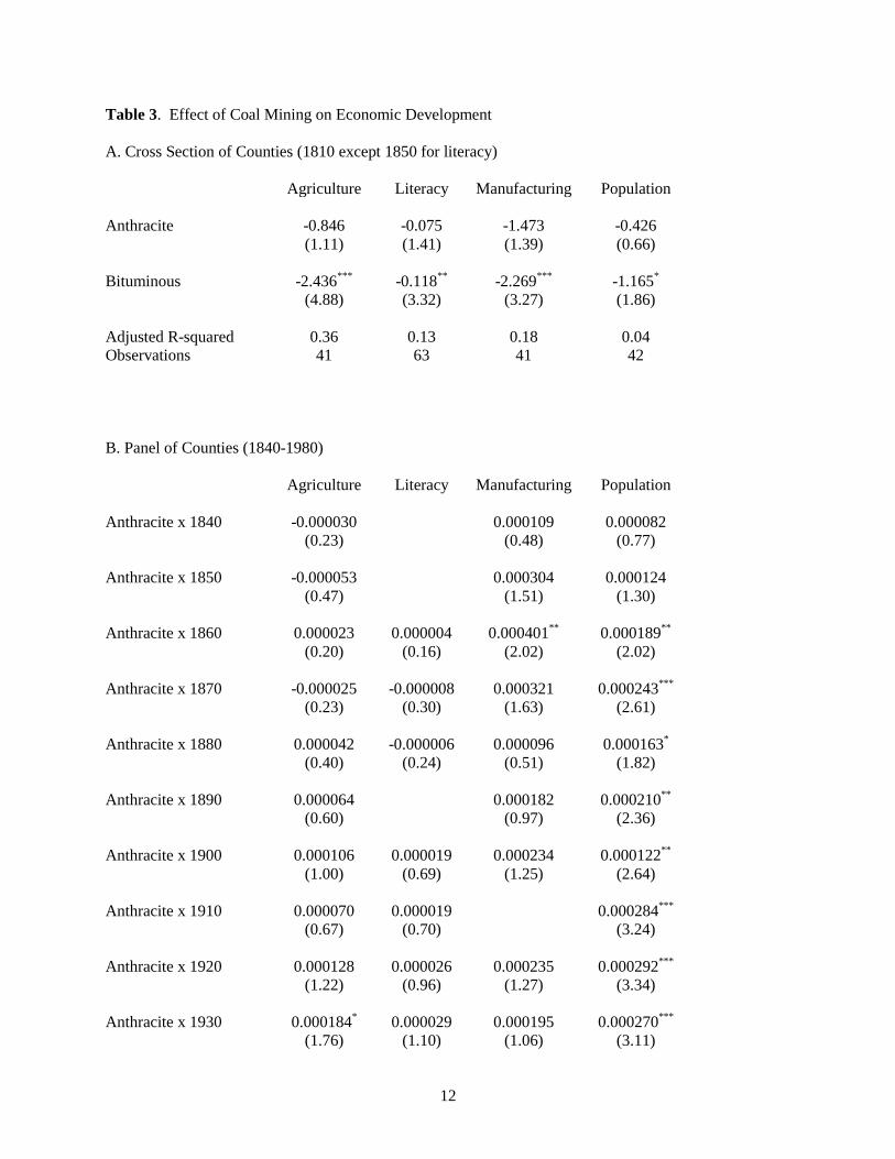
Table 3. Effect of Coal Mining on Economic Development
A. Cross Section of Counties (1810 except 1850 for literacy)
Agriculture Literacy Manufacturing Population
Anthracite -0.846 -0.075 -1.473 -0.426
(1.11) (1.41) (1.39) (0.66)
Bituminous -2.436***
-0.118**
-2.269***
-1.165*
(4.88) (3.32) (3.27) (1.86)
Adjusted R-squared 0.36 0.13 0.18 0.04
Observations 41 63 41 42
B. Panel of Counties (1840-1980)
Agriculture Literacy Manufacturing Population
Anthracite x 1840 -0.000030 0.000109 0.000082
(0.23) (0.48) (0.77)
Anthracite x 1850 -0.000053 0.000304 0.000124
(0.47) (1.51) (1.30)
Anthracite x 1860 0.000023 0.000004 0.000401**
0.000189**
(0.20) (0.16) (2.02) (2.02)
Anthracite x 1870 -0.000025 -0.000008 0.000321 0.000243***
(0.23) (0.30) (1.63) (2.61)
Anthracite x 1880 0.000042 -0.000006 0.000096 0.000163*
(0.40) (0.24) (0.51) (1.82)
Anthracite x 1890 0.000064 0.000182 0.000210**
(0.60) (0.97) (2.36)
Anthracite x 1900 0.000106 0.000019 0.000234 0.000122**
(1.00) (0.69) (1.25) (2.64)
Anthracite x 1910 0.000070 0.000019 0.000284***
(0.67) (0.70) (3.24)
Anthracite x 1920 0.000128 0.000026 0.000235 0.000292***
(1.22) (0.96) (1.27) (3.34)
Anthracite x 1930 0.000184* 0.000029 0.000195 0.000270
***
(1.76) (1.10) (1.06) (3.11)

13
Anthracite x 1940 0.000099 0.000293 0.000239***
(0.95) (0.16) (2.77)
Anthracite x 1950 0.000122 0.000105 0.000159*
(1.19) (0.57) (1.84)
Anthracite x 1960 0.000144 0.000111 0.000066
(1.40) (0.61) (0.77)
Anthracite x 1970 0.000048 0.000057 0.000008
(0.47) (0.31) (0.09)
Bituminous x 1840 0.000069 -0.000059 -0.000115
(0.79) (0.38) (1.58)
Bituminous x 1850 0.000170**
0.000036 -0.000004
(2.20) (0.26) (0.07)
Bituminous x 1860 0.000251***
0.000041**
-0.000094 0.000004
(3.31) (2.24) (0.69) (0.07)
Bituminous x 1870 0.000146**
0.000046**
0.000025 -0.000002
(1.96) (2.48) (0.19) (0.04)
Bituminous x 1880 0.000201***
0.000044**
0.000089 0.000067
(2.72) (2.40) (0.67) (1.10)
Bituminous x 1890 0.000198***
0.000194 0.000103*
(2.69) (1.48) (1.69)
Bituminous x 1900 0.000207***
0.000043**
0.000280**
0.000122**
(2.83) (2.38) (2.15) (2.02)
Bituminous x 1910 0.000235***
0.000044**
0.000174***
(3.23) (2.40) (2.89)
Bituminous x 1920 0.000220***
0.000047***
0.000274**
0.000190***
(3.03) (2.58) (2.12) (3.17)
Bituminous x 1930 0.000180**
0.000048***
0.000184 0.000150**
(2.50) (2.66) (1.43) (2.51)
Bituminous x 1940 0.000176**
0.000125 0.000144**
(2.46) (0.98) (2.43)
Bituminous x 1950 0.000041 0.000165 0.000102*
(0.57) (1.30) (1.72)
Bituminous x 1960 0.000099 0.000168 0.000045
(1.39) (1.33) (0.77)

14
Bituminous x 1970 -0.000003 0.000082 -0.000012
(0.04) (0.65) (0.20)
Adjusted R-squared 0.90 0.92 0.91 0.93
Observations 982 529 913 985
C. Cross Section of Counties (1980)
Agriculture Literacy Manufacturing Population
Anthracite -0.480 -0.124 -0.096
(1.20) (0.20) (0.20)
Bituminous -0.987***
-0.899**
-0.609*
(3.54) (2.16) (1.84)
Adjusted R-squared 0.14 0.04 0.02
Observations 65 63 67
Notes: Dependent variables are the natural logs of the density of the agricultural sector, the percentage of
the county population that can both read and write, the density of the manufacturing sector, and
population density. Panel regressions include county fixed effects and time effects. t-statistics are in
parentheses. ***
indicates significant at the 0.01 level. **
indicates significant at the 0.05 level. * indicates
significant at the 0.10 level.
where Yc is the natural log of the county-level outcome. Ac is a dummy variable with a value of 1 for
anthracite coal counties. Bc is a dummy variable with a value of 1 for bituminous coal counties, and c is
an error term.
In 1810, both the anthracite and bituminous coal industries were small and undeveloped.
Reassuringly for an attempt to uncover the impact of coal mining on economic outcomes, the anthracite
counties did not differ much at this time from the non-coal counties in agriculture, literacy,
manufacturing, and population density. The bituminous-producing counties, mostly located west of the
Alleghenies, were significantly less developed than the rest of the state in 1810, although Cuff’s (2006)
anthropometric data suggests that western Pennsylvanians enjoyed a higher standard of living prior to the
Civil War. This is not surprising as the frontier had moved west out of Pennsylvania only a decade before
(Florin 1977, p. 89).

15
Panel B in Table 2 shows the results from regressions of the form:
(2) Yct = c + t + Act + Bct + ct,
where Yct is the natural log of the economic outcome in county c in year t, c and t are county fixed
effects and year effects, and are time varying coefficients on the indicators for anthracite and
bituminous coal production, and ct is an error term.
Coal mining had a long-lived, positive impact on the economic development of both the
anthracite and bituminous regions of Pennsylvania. Mining is associated with a higher population
density, a proxy for the standard of living, from 1860 to 1950 among the anthracite counties and from
1890 to 1950 in the bituminous areas. While agricultural production and literacy rates in the anthracite
region were not significantly affected by mining, farming and human capital accumulation in the
bituminous region benefited mightily from mining. Taking county and time effects into account, in 1910
agricultural output per square mile was 56 percent higher and the literacy rate was 3 percentage points
higher in a typical bituminous county.
Coal mining did not crowd out manufacturing. At times there was a positive relationship between
coal production and manufacturing, but mining is mostly unrelated to manufacturing output. Anthracite
mining did have a positive impact early on. In 1860, the manufacturing density of a typical anthracite-
producing county was twice that of a similar non-coal county. Mining had its strongest impact on
manufacturing in the bituminous region between 1900 and 1920. The manufacturing density of a
bituminous-producing county was 70 greater than in an identical non-coal county in 1900.
Panel C in Table 3 shows the effects of coal mining in 1980 using the cross-section specification
in equation 1. By 1980, anthracite-producing counties were not experiencing significantly different
economic outcomes than non-coal producing counties. The bituminous coal counties were, however, less
developed than other counties in Pennsylvania in 1980. Population, manufacturing, and agricultural
densities were all lower in these counties. The manufacturing density in a bituminous-producing county
was 60 percent lower than in an otherwise similar county.

16
III. Discussion
The timing of the positive correlation between anthracite mining and manufacturing density in
1860 coincides with the rise of the anthracite iron industry. In 1850, there were 291 blast furnaces in
Pennsylvania, 57 of which used anthracite coal as a fuel (Convention of Iron Masters 1850). By 1858,
while blast furnaces in western Pennsylvania were still mostly burning charcoal those in eastern
Pennsylvania primarily burned anthracite coal (Knowles and Healey 2006, p. 613). There were 93
anthracite blast furnaces in Pennsylvania in 1858; 23 were located in anthracite-producing counties
(Lesley 1859). Lesley (1859) lists two anthracite furnaces in Carbon County, five in Columbia County,
six each in Dauphin and Luzerne Counties, and two each in Northumberland and Schuykill Counties.
There also were 10 rolling mills located in the anthracite region, one of which (located in Luzerne
County) produced 11,338 T-rails in 1856 (Lesley 1859, p. 236). The mines also provided a source of
demand as producing iron equipment for mining sustained several anthracite region iron makers (Powell
1980, p. 17-18).
However, the correlation between anthracite mining and manufacturing output was fleeting.
Anthracite iron furnaces were not concentrated in the coal fields but in the middle and lower Lehigh,
Schuykill, and Susquehanna River courses because raw material consumption was weighted heavily in
favor of ore rather than coal. Warren (1973, p. 19) argues that the lower river valleys of these rivers were
attractive to iron makers because there were deposits of iron ore (the ore resources of the anthracite fields
were small and high in silica), established charcoal iron works, and established markets (local mills and
foundries and in Philadelphia).
Improved rail access to the anthracite region lowered the relative price of coal in distant markets
thereby reducing the advantage of being located near the mines. While the Philadelphia and Reading
Railroad had completed its line from Pottsville in the Southern anthracite field to Philadelphia in 1842,
rail connections from the other anthracite fields were built in the 1850’s and 1860’s. The Delaware,
Lackawanna, and Western Railroad completed a line from Scranton north to a connection with the New
York and Erie Railroad in 1851 and a line from Scranton to the Delaware Water Gap in 1856 (Bogen

17
1927, p. 81 and 83). The Lehigh Valley Railroad opened a line from Mauch Chunk in the Middle coal
field to Easton in 1855 and extended the line to Wilkes-Barre in the Northern field in 1867 and to
Waverly, New York and an interchange with the Erie Railroad in 1869 (Bogen 1927, p. 112, 117, and
118). In 1871, the Central Railroad in New Jersey through the lease of the Lehigh and Susquehanna
Railroad created a line from Wilkes-Barre through the two northern coal fields to Jersey City (Bogen
1927, p. 158). The Delaware and Hudson Company finished a rail line from Carbondale in the Northern
field to the Erie Railroad’s main line at Lanesboro, Pennsylvania in 1870 and during the succeeding
decade built up a railroad system reaching to the Canadian border (Bogen 1927, p. 189). The effect of
these rail connections was to drive down the price of anthracite coal in Philadelphia and New York
relative to the price of coal at the mine. In 1840, the wholesale price of anthracite coal in Philadelphia
relative to the mine price was 3.6; by 1865 the ratio was 1.3 (Schaefer 1977, p. 216, 219, and 220).
Similarly, in New York the relative price fell from 5.3 in 1840 to 2.1 in 1863 (Schaefer 1977, p. 218-220).
Also, the dominance of anthracite coal as a blast furnace fuel was short lived. Between 1855 and
1870, anthracite smelted more than half of the iron produced in the United States (Powell 1980, p. 20).
But, in 1880, that share was down to 30 percent and by the turn of the twentieth century, less than 1
percent of pig iron production was fueled by anthracite (Warren 1973, p. 110). Cost considerations
contributed to the abandonment of anthracite coal by the iron industry in favor of bituminous coke. The
demand for anthracite as a domestic fuel kept its price fairly constant while “the feverish competition in
opening (bituminous) coal lands and marketing their product have caused an almost uninterrupted fall in
its price” (Taussig 1900, p. 147). In addition to the cost disadvantage, anthracite furnaces were also less
productive compared to those using coke because anthracite was not suitable for hard driving (Warren
2008, p. 11), a method of increasing the output of a furnace by blowing hot air through it at high pressure.
Anthracite mining had little long run impact on the manufacturing sectors of anthracite-abundant
counties and no significant effects on agriculture or the accumulation of human capital in those counties.
But, taking population density as being positively correlated with the standard of living, mining had a
positive effect on the economies of Pennsylvania’s anthracite region between 1860 and 1950. The

18
1950’s, punctuated by the Knox Mine Disaster in 1959 (Spohrer 1984; Wolensky et al. 1999) which led
directly to the closing of at least six deep mines and the loss of more than 1,000 jobs in the Northern field,
were a period of rapid decline in the anthracite industry. Production fell from 46 million net tons in 1950
to 18 million net tons in 1960; employment collapsed from 75,231 in 1950 to 20,269 in 1960 and then to
6,286 ten years later (Commonwealth of Pennsylvania 1974, p. 68).
The economic development of the bituminous coal counties was more closely tied to mining than
the development of the anthracite coal region. The bituminous counties, unsurprisingly as these were
among the last counties in Pennsylvania to be settled, initially lagged the rest of the state on all four
economic development metrics. Consistent with Sachs and Warner’s (2001, p. 833) hypothesis that
positive wealth shocks from the natural resource sector create an excess demand for non-traded goods,
coal mining encouraged the agricultural development of the bituminous region. Bituminous coal mining
was positively associated with agricultural density from 1850 until 1940. Also, the accumulation of
human capital, represented by the literacy rate, proceeded faster in the bituminous coal counties between
1860 and 1930, the final year analyzed for that variable.
Technological advances in the transportation and processing of agricultural output over the
second half of the nineteenth century meant that food no longer had to be locally grown. As new methods
of food processing, distribution, and storage were developed, marginal lands were taken out of
cultivation, leaving agricultural production increasingly concentrated on the most productive farmland. In
Pennsylvania the land in farms fell from 19,371,015 acres in 1900 to 14,112,841 acres in 1950, close to
the acreage a century earlier (Chen and Pasto 1955, p. 8). “The primary cause of this shrinkage was the
abandonment of rough or infertile land” (Fletcher 1955, p. 2).
Railroad construction was most rapid between 1850 and 1875. Rail transportation was available
during all seasons, which was not true of wagon or water transportation. Manufacturers and farmers had
a year-round market. Another advantage of railroads for farmers was their time-saving. Perishable
products such as milk, fruit, and vegetables could be marketed greater distances. The first shipment of
meat in refrigerated cars was in 1869, and a refrigerated car for transporting fruit was introduced in 1887
19
(Fletcher 1955, p. 237 and 279). Now, agricultural products could be shipped long distances. Southern
and Pacific coast produce became available in Pennsylvania markets, for example, beginning about 1885
(Fletcher 1955, p. 309).
Commercial canning began about 1890 and the quick freezing of vegetables started in 1931.
These developments enabled agricultural products to be transported and stored throughout the year. The
advent of good roads and motor vehicles in the early twentieth century permitted farmers to bring their
products to market themselves.
Over time, because of these improvements in food processing and distribution, agricultural
production concentrated in regions with the most productive farmland and land in the coal regions was
not especially fertile. Fletcher (1955, p. 24) describes the “blighting effect of coal mining on farming”
due to the land sinking or caving in above deep coal workings and the utter uselessness for agriculture of
land where strip mining was practiced. Coal mining polluted streams and the sulfuric acid gas fumes
from coke ovens killed all vegetation within an average distance of half a mile. Consequently, numerous
farms were abandoned in the coal region early in the twentieth century. A survey of farms in Blair
County found that one-fourth of the land in farms in 1900 was no longer farmed in 1940 (Fletcher 1955,
p. 5).
In Pennsylvania, gross farm production increased in the central and southeastern regions of the
state between 1899 and 1949 but decreased in the coal mining western and northern areas of the state
(Chen 1954, p. 410). The acreage of land in farms decreased 21 percent in the non-coal counties, 22
percent in the anthracite region, and 27 percent in the bituminous coal counties during the first half of the
twentieth century (Chen and Pasto 1955, p. 42).
By 1950, bituminous coal production was no longer statistically associated with agricultural
production. The introduction of refrigerated rail cars, the building of good roads and the development of
motor transportation, and the rise of commercial canning took the less productive farmland in
Pennsylvania out of cultivation. Production per acre of cropland in constant prices went from $15 in 1899
to $23 in 1949 (Chen and Pasto 1954, p. 26). This increase in agricultural productivity was most rapid in

20
the southeast portion of Pennsylvania and the slowest in the western bituminous-producing region,
leaving gross farm production per farm worker highest in the southeastern counties and lowest in the
bituminous coal counties (Chen 1954, p. 411). Crop production per acre was 68 percent higher in
southeastern Pennsylvania in 1949 than in the western region of the state (Chen and Pasto 1954, p. 37).
Just as in the anthracite region, mining had a fleeting statistically-detectable impact on the
manufacturing sectors of bituminous coal counties. Bituminous mining had a positive association with
manufacturing production between 1900 and 1920. This development was partially tied to the use of
bituminous coke as a fuel by the steel industry. Western Pennsylvania iron makers were slow to adopt
mineral fuels (Knowles and Healey 2006), but by 1880, 40 percent of pig iron was produced using
bituminous coke (Warren 1973, p. 110). The dominance of bituminous coke came quickly. In 1890, 71
percent of pig iron production was smelted with bituminous coke (Warren 1973, p. 110). In 1900, that
percentage was 85 percent and, in 1905, 90 percent of pig iron was produced using bituminous coke
(Warren 1973, p. 110). By the early 1900’s, western Pennsylvania industry was the steel industry. In
1905, the value of all Pittsburgh manufactures was $164.4 million; $89.4 million of that was the output of
its iron and steel industry (Warren 1973, p. 120).
An anonymous (1889, p. 409) commenter predicted that “(t)he history of iron-making leads us to
expect that here, as in other countries, the ore will move to the fuel, and not the fuel to the ore.” This was
true for other industries as well. The early manufacturing establishments in western Pennsylvania,
breweries, glassworks, foundries, and machine shops used bituminous coal as their principal fuel and
were located near easily accessible supplies (Binder 1974, p. 42).
Access to bituminous coal was critical for economic development at the turn of the twentieth
century. In 1900, 56.6 percent of aggregate energy consumption in the United States was supplied by
bituminous coal; in 1910, the percentage was 64.3 and in 1920, 62.3, with nearly two-thirds of the coal
used for industrial purposes (Schurr and Netschert 1960, p. 36 and 76). From 1900 to 1920, the period
when bituminous coal mining is positively and significantly correlated with manufacturing production,
the U.S. showed a rising trend of energy consumption relative to output. Using 1900 as a base year, an
21
index of total energy consumption per unit of GNP rose to 116.8 in 1910 and was 116.2 in 1920 (Schurr
and Netschert 1960, p. 524-525). The increasing importance of access to cheap bituminous coal around
the turn of the last century is especially noticeable in an index of coal consumption per unit of GNP,
which has a value of 100 in 1900, 125.7 in 1910, and 118.1 in 1920 (Schurr and Netschert 1960, p. 524-
525).
A structural shift in industrial energy requirements apparently took place after 1920. While the
index of total energy consumption per unit of GNP declined from 99.3 in 1930 to 74.7 in 1950, the index
of coal input per unit of GNP fell from 80.1 to 38.5 over that same period (Schurr and Netschert 1960, p.
524-525). Access to coal was no longer important for manufacturing. Friscia (1970, p. 49) argues that
there was a decreased demand for coal in industrial uses where increased productivity in fuel usage was
an important cost concern. Industrial users substituted liquid and gas fuels for coal. An index of coal
consumed by manufacturing per unit of manufacturing output stood at 100 in 1909, 81.6 in 1919, 54.5 in
1929, 38.5 in 1939, and 21.3 in 1954 (Schurr and Netschert 1960, p. 79).
Technological change reduced the advantages of being located near the bituminous mines in other
ways as well. By-product coking reduced the cost of fuel for coke ovens remote from the industry’s
home in Connellsville in Fayette County, Pennsylvania, allowing for the use of poorer quality coal
(Warren 1973, p. 115). This helped disperse the steel industry from around Pittsburgh. So, by 1920, the
Pittsburgh mills had become the high cost producers. The mill cost at U.S. Steel’s Pittsburgh works was
$52.20 a ton compared to $42.80 in Chicago (Warren 1973, p. 178). Western Pennsylvania mills had
remained competitive thanks to U.S. Steel’s “Pittsburgh Plus” pricing scheme which set the price of steel
anywhere in the country equal to the price in Pittsburgh plus the shipping cost from Pittsburgh. This
enabled Pittsburgh steel mills to offer equal competition anywhere in the United States in terms of
delivered price. Pittsburgh Plus pricing gave steel fabricators an incentive to locate in western
Pennsylvania since steel prices were lowest in Pittsburgh. In 1920, a Pittsburgh structural steel fabricator
could obtain steel for $7.60 a ton less than a Chicago competitor and was thus able to win contracts in
Chicago (Warren 1973, p. 201).

22
Pittsburgh Plus pricing was in effect from 1909 to 1924 when the FTC ordered U.S. Steel to cease
the practice of selling everywhere based on the Pittsburgh price. Immediately, a shift in finished steel
production took place inside Pennsylvania itself. In 1920, 48.5 percent of total Pennsylvania production
of rolled iron and steel occurred in Allegheny County and 6.2 percent in Lehigh and Northampton
Counties in eastern Pennsylvania; in 1925, 43.7 percent was rolled in Allegheny County and 9.7 percent
in those two Lehigh Valley counties (Warren 1973, p. 201).
IV. Summary
Coal mining did not harm the long run development of Pennsylvania’s anthracite and bituminous
regions. Coal mining is not associated with negative economic outcomes. Instead, from the Civil War
through the Second World War, mining positively impacted the economies of the state’s coal counties,
with population density, a proxy for the standard of living, being significantly higher in these counties.
As manufacturing production became more energy-intensive in the late nineteenth and early twentieth
centuries, proximity to cheap coal became an important cost consideration. Fuel-intensive industries such
as steel concentrated in the western Pennsylvania bituminous coal fields. With the declining importance
to manufacturing of energy inputs in general and coal in particular after 1920, the economies of
Pennsylvania’s coal counties gradually came to look no different than the state’s non-coal counties. The
poor relative economic performance of the state’s bituminous counties is a recent phenomenon and
occurred long after coal mining ceased to be an important contributor to the region’s economies. By
1980, mining of all kinds comprised just 2.4 percent of private employment in the coal regions of
Pennsylvania.
23
References
Adams, Sean Patrick. Old Dominion, Industrial Commonwealth: Coal, Politics, and Economy in
Antebellum America. Baltimore, MD: Johns Hopkins University Press, 2004.
Anonymous. “Notes and Memoranda.” Quarterly Journal of Economics 3(4), July 1889, p. 497-499.
Aurand, Harold. “Diversifying the Economy of the Anthracite Region, 1880-1900.” Pennsylvania
Magazine of History and Biography 94(1), January 1970, p. 54-61.
Auty, Richard M. “Introduction and Overview.” in R.M. Auty (ed.) Resource Abundance and Economic
Development. Oxford: Oxford University Press, 2001, p. 3-16.
Beeson, Patricia E., David N. DeJong, and Werner Troesken. “Population Growth in U.S. Counties, 1840-
1990.” Regional Science and Urban Economics 31(6), November 2001, p. 669-699.
Billinger, Robert D. Pennsylvania’s Coal Industry. Gettysburg, PA: Pennsylvania Historical Association,
1954.
Binder, Frederick Moore. Coal Age Empire: Pennsylvania Coal and Its Utilization to 1860. Harrisburg,
PA: : Pennsylvania Historical and Museum Commission, 1974.
Bogen, Jules I. The Anthracite Railroads: A Study in American Railroad Enterprise. New York: Ronald
Press, 1927.
Chandler, Alfred D. “Anthracite Coal and the Beginnings of the Industrial Revolution in the United
States.” Business History Review 49(2), Summer 1972, p. 141-181.
Chen, Kuan-I. Agricultural Production in Pennsylvania, 1840 to 1950. Ph.D. dissertation, Pennsylvania
State University, 1954.
Chen, Kuan-I and Jerome K. Pasto. Facts on a Century of Agriculture in Pennsylvania 1839 to 1950.
State College, PA: Pennsylvania State University College of Agriculture Agricultural Experiment
Station, 1955.
Commonwealth of Pennsylvania. Department of Environmental Resources Annual Report on Mining, Oil
and Gas, and Land Reclamation and Conservation Activities. Harrisburg, PA: Commonwealth of
Pennsylvania, 1974.
Commonwealth of Pennsylvania. Reports of the Inspectors of Mines of the Anthracite and Bituminous
Coal Regions of Pennsylvania, for the Year 1891. Harrisburg, PA: Edwin K. Meyers, 1892.
Convention of Iron Masters. Documents Relating to the Manufacture of Iron in Pennsylvania. Published
on Behalf of the Convention of Iron Masters, Which Met in Philadelphia, On the Twentieth of
December, 1849. Philadelphia, PA: The General Committee, 1850.
Coxe, Tench. A Statement of the Arts and Manufactures of the United States of America for the Year
1810. Philadelphia, PA: A. Cornman, 1814.
Cuff, Timothy. “Anthropometric History: What is It and What Can It Tell Us About Antebellum
Pennsylvania?” Pennsylvania History 73(2), Spring 2006, p. 143-197.

24
DiCiccio, Carmen. Coal and Coke in Pennsylvania. Harrisburg, PA: Pennsylvania Historical and
Museum Commission, 1996.
Dublin, Thomas and Walter Light. The Face of Decline: The Pennsylvania Anthracite Region in the
Twentieth Century. Ithaca, NY: Cornell University Press, 2005.
Easterlin, Ricard A., “Interregional Differences in Per Capita Income, Population, and Total Income,
1840-1950”, inTrends in the American Economy in the Nineteenth Century, Conference on
Research in Income and Wealth (eds.), Princeton, NJ: Princeton University Press, 1960,
p. 73-140.
Eavenson, Howard N. The First Century and a Quarter of American Coal Industry. Pittsburgh, PA:
Privately Printed, 1942.
Edmunds, William E. Coal Reserves of Pennsylvania: Total, Recoverable, and Strippable (January 1,
1970). Harrisburg, PA: Pennsylvania Geological Survey, 1972.
Ellison, Glenn and Edward L. Glaeser. “The Geographic Concentration of Industry: Does Natural
Advantage Explain Agglomeration?”American Economic Review 89(2), May 1999, p. 311-316.
Fletcher, Stevenson Whitcomb. Pennsylvania Agriculture and Country Life, 1840-1940. Harrisburg, PA:
Pennsylvania Historical and Museum Commission, 1955.
Florin, John. “The Advance of Frontier Settlement in Pennsylvania, 1638-1850: A Geographic
Interpretation.” Papers in Geography No. 14, Department of Geography, Pennsylvania State
University, May 1977.
Friscia, August Blake. Industrial Retardation and Economic Growth: A Case Study of Secular and
Structural Change in the Bituminous Coal Industry of the United States, 1920-1960. Ph.D.
Dissertation, New York University, 1970.
Goldstein, G. S. and T. J. Gronberg, “Economies of Scope and Economies of Agglomeration.” Journal of
Urban Economics 16, 1984, p. 91-104.
Gylfason, Thorvaldur, Tryggvi Thor Herbertsson, and Gylfi Zoega. “A Mixed Blessing.” Macroeconomic
Dynamics 3, 1999, p. 204-225
Habakkuk. H. J. American and British Technology in the Nineteenth Century: The Search for Labor-
Saving Inventions. Cambridge: Cambridge University Press, 1962.
Healey, Richard G. The Pennsylvania Anthracite Coal Industry, 1860-1902: Economic Cycles, Business
Decision-Making and Regional Dynamics. Scranton, PA: University of Scranton Press, 2007.
Helsley, Robert W. amd William C. Strange, “Matching and Agglomeration Economies in a System of
Cities.” Regional Science and Urban Economics 20, 1990, p. 189-212.
Hoffman, John N. “Pennsylvania’s Bituminous Coal Industry: An Industry Review.” Pennsylvania
History 45(4), October 1978, p. 351-363.
Hudson Coal Company. The Story of Anthracite. New York: Hudson Coal Company, 1932.

25
Jones, Chester Lloyd. The Economic History of the Anthracite-Tidewater Canals. Philadelphia, PA:
University of Pennsylvania, 1908.
Knowles, Anne Kelly and Richard G. Healey. “Geography, Timing, and Technology: A GIS-Based
Analysis of Pennsylvania’s Iron Industry, 1825-1875.” Journal of Economic History 66(3),
September 2006, p. 608-634.
Lesley, J. P. The Iron Manufacturer’s Guide to the Furnaces, Forges and Rolling Mills of the United
States. New York: John Wiley, 1859.
Lindstrom, Diane. Economic Development in the Philadelphia Region, 1810-1850. New York: Columbia
University Press, 1978.
Michaels, Guy. “The Long Term Consequences of Regional Specialization.” London School of
Economics and Political Science, Centre for Economic Performance Discussion Paper No. 766,
December 2006.
Miller, Donald L. and Richard E. Sharpless. The Kingdom of Coal: Work, Enterprise, and Ethnic
Communities in the Mine Fields. Philadelphia: University of Pennsylvania Press, 1985.
Mitchener, Kris James and Ian W. McLean. “The Productivity of U.S. States since 1880.” Journal of
Economic Growth 8(1), 2003, p. 73-114.
Papyrakis. Elissaios and Reyer Gerlagh. “Resource Abundance and Economic Growth in the United
States”. European Economic Review 51, 2007, p. 1011-1039.
Pennsylvania Department of Environmental Resources. Annual Report on Mining Activities. Harrisburg,
PA: Pennsylvania Department of Environmental Resources, 1980.
Pennsylvania Department of Mines. History of Pennsylvania Bituminous Coal. Harrisburg, PA:
Pennsylvania Department of Mines, 1955.
Powell, H. Benjamin. “The Pennsylvania Anthracite Industry, 1769-1976.” Pennsylvania History 47(1),
January 1980, p. 3-28.
Rappaport, Jordan and Jeffrey D. Sachs. “The United States as a Coastal Nation.” Journal of
Economic Growth 8(1), March 2003, p. 5-46.
Robinson, James A., Ragnar Torvick, and Thierry Verdier. “Political Foundations of the Resource
Curse.” Journal of Development Economics 79, 2006, p. 447-468.
Rosenthal, Stuart S. and William C. Strange, “The Determinants of Agglomeration.” Journal of Urban
Economics 50, 2001, 191-229.
Ruggles, Steven, Matthew Sobek, Trent Alexander, Catherine A. Fitch, Ronald Goeken, Patricia Kelly
Hall, Miriam King, and Chad Ronnander. Integrated Public Use Microdata Series: Version 4.0.
Minneapolis, MN: Minnesota Population Center, 2008.
Sachs, Jeffrey D. and Andrew W. Warner. “The Big Push, Natural Resource Booms and Growth.”
Journal of Development Economics 59, 1999, p. 43-76.

26
Sachs, Jeffrey D. and Andrew W. Warner. “The Curse of Natural Resources.” European Economic
Review 45(4-6), May 2001, p. 827-838.
Schaefer, Donald Fred. A Quantitative Description and Analysis of the Growth of the Pennsylvania
Anthracite Coal Industry 1820 to 1865. New York: Arno Press, 1977.
Schurr, Sam H. and Bruce C. Netschert. Energy in the American Economy, 1850-1975: An Economic
Study of its History and Prospects. Baltimore, MD: Johns Hopkins University Press, 1960.
Seaman, Ezra C. Supplement No. 11 to Essays on the Progress of Nations in Productive Industry,
Civilization, Population, and Wealth. New York: Baker and Scribner, 1848.
Spohrer, George A. “The Knox Mine Disaster: The Beginning of the End.” Proceedings and Collections
of the Wyoming Historical and Geological Society 1984, p. 124-145.
Taussig, F. W. “The Iron Industry in the United States.” Quarterly Journal of Economics 14(2), February
1900, p. 143-170.
Thorndale, William and William Dollarhide. Map Guide to the U.S. Federal Censuses, 1790-1920.
Baltimore, MD: Genealogical Publishing, 1987.
Tucker, George. Progress of the United States in Population and Wealth in Fifty Years As Exhibited by
the Decennial Census from 1790 to 1840. New York: Press of Hunt’s Merchant’s Magazine,
1855.
Warren, Kenneth. Bethlehem Steel: Builder and Arsenal of America. Pittsburgh, PA: University of
Pittsburgh Press, 2008.
Warren, Kenneth. The American Steel Industry 1850-1970: A Geographical Interpretation. Oxford:
Clarendon Press, 1973.
Wolensky, Robert P., Kenneth C. Wolensky, and Nicole H. Wolensky. The Knox Mine Disaster: The
Final Years of the Northern Anthracite Industry and the Effort to Rebuild a Regional Economy.
Harrisburg, PA: Pennsylvania Museum and Historical Commission, 1999.
Wright, Gavin. “The Origins of American Industrial Success, 1879-1940.” American Economic Review
80(4), September 1990, p. 651-668.
Wright, Gavin and Jesse Czelusta. “The Myth of the Resource Curse.” Challenge 47(2), March/April
2004, p. 6-38.