CO2 Injection Into a Deep Saline Aquifer: Porosity ...

University of Tennessee, Knoxville University of Tennessee, Knoxville

TRACE: Tennessee Research and Creative TRACE: Tennessee Research and Creative

Exchange Exchange

Masters Theses Graduate School

12-2012

CO2 Injection Into a Deep Saline Aquifer: Porosity Measurements, CO2 Injection Into a Deep Saline Aquifer: Porosity Measurements,

Numerical Modeling, and Costs Associated with Uncertainty of Numerical Modeling, and Costs Associated with Uncertainty of

Petrophysical Parameters Petrophysical Parameters

Michael John Gragg [email protected]

Follow this and additional works at: https://trace.tennessee.edu/utk_gradthes

Part of the Geology Commons, Natural Resource Economics Commons, Oil, Gas, and Energy

Commons, and the Sustainability Commons

Recommended Citation Recommended Citation Gragg, Michael John, "CO2 Injection Into a Deep Saline Aquifer: Porosity Measurements, Numerical Modeling, and Costs Associated with Uncertainty of Petrophysical Parameters. " Master's Thesis, University of Tennessee, 2012. https://trace.tennessee.edu/utk_gradthes/1380

This Thesis is brought to you for free and open access by the Graduate School at TRACE: Tennessee Research and Creative Exchange. It has been accepted for inclusion in Masters Theses by an authorized administrator of TRACE: Tennessee Research and Creative Exchange. For more information, please contact [email protected].

https://trace.tennessee.edu/

https://trace.tennessee.edu/

https://trace.tennessee.edu/utk_gradthes

https://trace.tennessee.edu/utk-grad

https://trace.tennessee.edu/utk_gradthes?utm_source=trace.tennessee.edu%2Futk_gradthes%2F1380&utm_medium=PDF&utm_campaign=PDFCoverPages

http://network.bepress.com/hgg/discipline/156?utm_source=trace.tennessee.edu%2Futk_gradthes%2F1380&utm_medium=PDF&utm_campaign=PDFCoverPages





mailto:[email protected]

To the Graduate Council:

I am submitting herewith a thesis written by Michael John Gragg entitled "CO2 Injection Into a

Deep Saline Aquifer: Porosity Measurements, Numerical Modeling, and Costs Associated with

Uncertainty of Petrophysical Parameters." I have examined the final electronic copy of this

thesis for form and content and recommend that it be accepted in partial fulfillment of the

requirements for the degree of Master of Science, with a major in Geology.

Edmund Perfect, Major Professor

We have read this thesis and recommend its acceptance:

Larry D. McKay, Peter J. Lemiszki

Accepted for the Council:

Carolyn R. Hodges

Vice Provost and Dean of the Graduate School

(Original signatures are on file with official student records.)

CO2 Injection Into a Deep Saline Aquifer: Porosity Measurements, Numerical Modeling, and Costs Associated with Uncertainty of Petrophysical Parameters

A Thesis Presented for the Master of Science Degree The University of Tennessee, Knoxville

Michael John Gragg December 2012

ii

Acknowledgments

I would first like to thank my wife, Gretchen, for her unending support through the

years of education that have brought me here. She has encouraged me, taken care of our

boys, and at times completely supported us financially. Without her none of this would

have been possible. I would also like to thank my two boys, Elijah and Yohan, for the joy

that they bring into my life. Also, my parents, John and Elizabeth, deserve a huge thank you

for supporting my interests and me as I was growing up.

Dr. Edmund Perfect has been a wonderful advisor and holds an enormous amount of

my gratitude for his guidance and patience over the past few years. From the first time I

visited with him, over a year before starting graduate school, he has been helpful and kind,

directing me through the transition from undergraduate to graduate student. I would also

like to thank Chu-‐Lin “Mike” Cheng for all of his help with the STOMP simulator, for sharing

his expertise, advice, teakettle, and for helping me find answers to my many questions. Ken

Christle also deserves a huge thank you for helping run some of the STOMP simulations

over the summer of 2012 and helping to trouble shoot when problems arose. Thanks also

to my committee members, Dr. Larry McKay and Dr. Peter Lemiszki, for their timely replies

to my questions and many helpful suggestions. Thanks to Dr. Colin Sumrall and Will

Atwood for providing training and use of the NextEngine 3D desktop laser scanner. I would

also like to thank the faculty and graduate students of the Earth and Planetary Sciences

Department at UT for making my time in Knoxville so enjoyable.

My funding, for which I am eternally grateful, has come from the University of

Tennessee, Knoxville, Earth and Planetary Sciences Department and from the Tennessee

Division of Geology.

iii

Abstract

Anthropogenic levels of atmospheric greenhouse gases, particularly carbon

dioxide (CO2) have increased rapidly over the last several decades and coincide with rising

temperatures globally. One possible solution is to capture CO2 before it is released into the

atmosphere by large point sources, such as fossil fuel power plants. Once captured, the CO2

can be condensed and transported to a storage facility. Of the available options for storage

of condensed CO2, geologic sequestration in deep saline aquifers is considered the most

viable option.

Porosity measurements were obtained for nearly 100 core samples of the Knox and

Stones River groups from the middle Tennessee area as part of a larger project for the

Tennessee Division of Geology, characterizing the potential for geologic CO2 sequestration

in Tennessee. Certain formations within these groups were found to exhibit higher porosity

(higher storage potential) than others. Measured porosity values were quite low, ranging

from 0.21 – 10.67 % with a median value of 1.21 %. These data can be used to aid in the

decision-‐making process concerning possible geologic targets for geologic CO2

sequestration in Tennessee.

A sensitivity analysis was also performed using a numerical model for geologic

carbon sequestration (STOMP). Intrinsic permeability, porosity, pore compressibility, the

van Genuchten residual liquid saturation, α and m parameters, and the Brooks and Corey

residual liquid and gas saturations were varied independently and their influence on CO2

storage was determined. Changes in costs based on the parameter variations were

calculated to evaluate the relative importance of the various parameters. The most

influential parameters were intrinsic permeability, the van Genuchten m parameter, and

iv

the Brooks and Corey residual gas saturation. These results highlight the need for accurate

measurement of intrinsic permeability and capillary pressure-‐saturation parameters in

addition to more commonly measured properties like porosity.

v

Table of Contents

Section Page

Chapter 1 – General Introduction…...………………………………………………………………… 1

Chapter 2 – Determination of Porosity………...……………………………………………………. 5

2.1 Introduction…………………………………………………………………………………………….. 5

2.2 Methodology………………………...………………………………………………………………….. 7

2.3 Results and Discussion..……………………………………………………………………………. 9

2.4 Conclusions……………………………………………………………………………………………… 11

Chapter 3 – Numerical Modeling and Cost Estimates…………………………………………. 13

3.1 Introduction………….…………………………………………………………………………………. 13

3.2 Methodology..…………………………………………………………………………………………... 19

3.3 Results…………………………………………………………………………………………………….. 24

3.4 Conclusions……………………………………………………………………………………………… 29

Chapter 4 – General Conclusions………………………....……………………………………………. 30

List of References...…………………….……………………………………………………….…………….. 32

Appendices……………………………………………………………………………………….…………….... 40

Appendix 1 – Tables……………………………………………………………………...………………. 41

Appendix 2 – Figures…………………………………………………………………………………….. 50

Appendix 3 – Raw Porosity Data……………………….…...………………………………………. 64

Appendix 4 – Example STOMP Input File…...…………...…………………………...…………. 67

Appendix 5 – Summary of STOMP Simulations….……………………………………………. 70

Vita…………………………………………………………………………………………………………………... 98

vi

List of Tables

Table Page

Table 1 –CO2 Trapping Mechanisms…………………………………….….………………………… 41

Table 2 – Sample Mass Reproducibility…………...………………….….…………………………. 42

Table 3 – Core Volume Measurement Reproducibility………....….…………………………. 43

Table 4 – Porosity Above and Below 800 m Depth………...….…….…………………………. 44

Table 5 – Porosity by Formation……….………...……………………………………………………. 45

Table 6 – Input Parameters for the Numerical Model..………………………………..……… 46

Table 7 – Injection Rates and Costs……………...……………………………………………………. 47

Table 8 – Parameter, Cost, and Normalized Coefficients of Variation…………….……. 49

vii

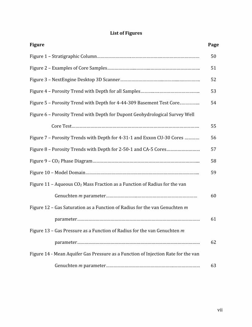
List of Figures

Figure Page

Figure 1 – Stratigraphic Column……………………….…………………….………………………… 50

Figure 2 – Examples of Core Samples…………………...………...…………………………………. 51

Figure 3 – NextEngine Desktop 3D Scanner……………………………...………....….…………. 52

Figure 4 – Porosity Trend with Depth for all Samples………...….……………………….….. 53

Figure 5 – Porosity Trend with Depth for 4-‐44-‐309 Basement Test Core..…………... 54

Figure 6 – Porosity Trend with Depth for Dupont Geohydrological Survey Well

Core Test………………………………………………………………………………………….

55

Figure 7 – Porosity Trends with Depth for 4-‐31-‐1 and Exxon CU-‐30 Cores ………… 56

Figure 8 – Porosity Trends with Depth for 2-‐50-‐1 and CA-‐5 Cores……………………… 57

Figure 9 – CO2 Phase Diagram…………………………………………………………………………... 58

Figure 10 – Model Domain……………………………………………………………………………….. 59

Figure 11 – Aqueous CO2 Mass Fraction as a Function of Radius for the van

Genuchten m parameter……………………..…………………………………………

60

Figure 12 – Gas Saturation as a Function of Radius for the van Genuchten m

parameter………………………………………………………………………………………

61

Figure 13 – Gas Pressure as a Function of Radius for the van Genuchten m

parameter………………………………………………………………………………………

62

Figure 14 -‐ Mean Aquifer Gas Pressure as a Function of Injection Rate for the van

Genuchten m parameter……………………………………………….…………………

63

1

Chapter 1 – General Introduction

Anthropogenic levels of atmospheric greenhouse gases, particularly carbon dioxide

(CO2), have increased rapidly over the last several decades and coincide with rising

temperatures globally. According to Sundquist et al. (2008), CO2 concentrations in the

atmosphere have risen from around 280 ppm to over 380 ppm in the last 250 years,

inducing measureable increases in global temperature. Concerns over regional air quality

and global warming have resulted in the need to evaluate alternative methods for dealing

with CO2 and other airborne emissions from various sources. One possible alternative is to

capture CO2 before it is released into the atmosphere by large point sources such as fossil

fuel power plants and cement operations. Once captured, the CO2 can be condensed and

transported to a storage facility. There are several options for storing condensed CO2

including mineralization in the form of stable carbonates, deep ocean sequestration, and

sequestration in geologic material at depth. Of these, geologic storage is considered the

most viable option (Yang et al., 2010; Celia and Nordbotten, 2009). In order for site specific

or regional investigations to take place a basic understanding of the available geologic

reservoirs and their hydraulic and storage properties is required.

There are several options for deep geologic storage: depleted oil and gas reservoirs;

unmineable coal seams; and deep saline aquifers. The technology for carbon capture and

storage already exists and is currently implemented by the oil and natural gas industries

for enhanced oil and natural gas recovery as well as for temporary storage of natural gas

(Solomon et al., 2008; Pacala and Socolow, 2004). Carbon dioxide stored in unmineable

coal beds can enhance coal bed methane extraction while sequestering the CO2 through

displacement of the methane (Klara et al., 2003). Finally, deep saline aquifers seem to be

2

the most attractive targets for carbon sequestration since they are normally unused due to

high salinity, typically have high storage capacity, and are readily available (Yang et al.,

2010; Pruess et al., 2003).

In order for a deep saline reservoir to function as a storage site the CO2 must meet

several requirements. One of these requirements is that the target unit is at a minimum

depth of 800 meters (2625 feet). This ensures the best storage conditions by assuring that

the CO2 remains in a supercritical state at which CO2 becomes dense like a liquid with gas-‐

like viscosity, allowing a much higher mass of CO2 to be stored in a given volume. Also, CO2

must remain in the formation for many years. This is accomplished by several trapping

mechanisms that operate on differing time and spatial scales. These mechanisms include

structural and stratigraphic trapping, residual gas trapping, solubility trapping, and

mineral trapping (Bradshaw et al., 2007). Structural and stratigraphic traps exist due to the

geologic structures within the reservoir (folds, faults, etc.) and the buoyancy contrast

between the CO2 and surrounding brine. Residual gas trapping takes place as CO2 becomes

trapped in the pore space of the reservoir rock as the plume migrates away from the

injection well. Over the course of many years, as the CO2 migrates, it also begins to dissolve

into the reservoir brine. This is known as solubility trapping. Over large time scales mineral

trapping can become substantial as the CO2 chemically reacts with the reservoir rock

minerals and the brine. These trapping mechanisms are summarized in table 1, which was

modified from Bradshaw et al. (2007).

This thesis focuses on geologic sequestration of CO2 in deep saline aquifers and is

divided into several sections. The first section centers around porosity measurements

made for the Tennessee Division of Geology as part of a larger project (Subcontract

3

#32701-‐00962, Edison Record ID 28407) to estimate the potential for geologic carbon

sequestration in Tennessee. This project involved nearly 100 core samples from the middle

Tennessee area taken from the Knox and Stones River groups, consisting predominantly of

carbonate rocks (limestones and dolostones with minor sandstones and shales).

Measurements involved creating a three-‐dimensional scan of each core in order to obtain

bulk volume data and weighing each sample under both oven-‐dry and water-‐saturated

conditions in order to determine the porosity of each sample.

The overall goal of the first section was to characterize prospective geologic

reservoirs in Tennessee. This goal can be broken down into two main objectives:

• Measurement of matrix porosity of rock cores from units of interest

• Identification of specific formations of high potential storage volume

The hypothesis for the project was simply that measured porosity values would be

significantly higher for some formations than others.

The second section focuses on a sensitivity analysis of a numerical model for

geologic carbon sequestration (STOMP), to examine the relative influence of input

parameters on CO2 storage. In this section multiple petrophysical input parameters were

varied independently. The parameters investigated were intrinsic permeability, porosity,

pore compressibility, the van Genuchten α parameter, the van Genuchten m parameter, the

van Genuchten residual liquid saturation, the Brooks and Corey residual liquid saturation,

and the residual gas saturation. The model outputs were analyzed to quantify the impact of

geologic heterogeneity and measurement accuracy on injection costs.

The goal of this research was to examine the relative importance of different input

parameters for numerical simulation of CO2 storage in geologic reservoirs. This will help

4

future researchers focus on obtaining accurate estimates of parameters that have the

greatest effect on the simulation while spending less time and money on those which are

less significant. This study should help to:

• Identify parameters that have the greatest impact on simulation results (these

influential parameters should therefore be most accurately estimated);

• Identify parameters that are less influential to the simulation results (these

parameters could therefore be less accurately estimated);

• Demonstrate the usefulness of numerical models in predicting costs associated

carbon dioxide capture and storage.

These objectives can be rewritten in the form of two hypotheses. First, that certain

parameters, most likely intrinsic permeability and porosity, will show significantly more

influence on model outputs than others. Second, that variations of influential parameters

will result in significant changes in the cost of CO2 injection.

The final section summarizes conclusions of the study and outlines possible

directions for future work.

5

Chapter 2 – Determination of Porosity

2.1 Introduction

Porosity, defined as the ratio of void space within a rock to the total rock volume, is

of great importance in regards to storage volume potential. This void volume is the basis

for estimating the amount of a given substance, such as supercritical CO2, that can be stored

within a reservoir. There are multiple methods for measuring porosity including mercury

intrusion porosimetry, gas expansion, computed tomography and the wet and dry weight

method, described later in this chapter (Franklin, 1972; Goldstrand et al., 1995; Kazimierz

et al., 2004).

Because porosity is a basic petrophysical parameter required for modeling injection

of CO2 into an aquifer, an estimate of porosity is required before beginning any simulation.

Estimates of porosity can come from the literature or from some form of measurement. For

example, some researchers have used computed tomography to estimate porosity changes

due to different CO2 injection rates (Izgec et al., 2005). Others have used geophysical data

from injection wells calibrated to porosity measurements from core samples to determine

inputs for numerical models of the Frio Brine Test pilot site in Texas, USA (Sakurai et al.,

2005; Doughty et al., 2008). Similarly, Gupta et al. (2008) measured porosity for the Rose

Run and Copper Ridge Formations in the Ohio River Valley from geophysical logs and from

core samples using mercury injection. Conversely, in their analysis of basin-‐scale storage

potential, Szulczewski and Juanes (2009) estimated the porosity of the Fox Hill sandstone

in the Powder River Basin using the only available published estimate. Recently, Koperna et

al. (2012) used geophysical data as well as core samples to determine porosity of the

Paluxy sandstone at the SECARB Anthropogenic Test R&D site near Bucks, Alabama, USA.

6

In more theoretical approaches an estimation of porosity is used with the assumption that

this value falls within an acceptable range of porosity values, typically between 10% and

20% (Pruess et al., 2002). Regardless of the methods used, an estimation of porosity is

absolutely necessary for simulating geologic sequestration of CO2 in saline aquifers.

Simply put, an understanding of the petrophysical properties of available geologic

reservoirs is necessary for any regional or site-‐specific study to take place. To that end,

porosity measurements on core samples were made as part of a larger project through the

Tennessee Division of Geology to characterize the potential for geologic carbon storage in

Tennessee. These porosity values are needed to evaluate the volume of CO2 that can be

stored within a given geologic formation

The overall goal of the project was to characterize prospective geologic reservoirs in

Tennessee. This goal was broken down into several objectives:

• Measurement of matrix porosity of rock core from units of interest

• Identification of specific formations of high potential storage volume

The hypothesis for the project was simply that measured porosity values would be

significantly higher for some formations than others.

For this first study the Knox (K) and Stones River (SR) groups, west of the

Cumberland Plateau-‐Valley and Ridge province boundary, were considered to be the most

promising storage assessment units (SAU) in Tennessee (see figure 1). Little to no data

currently exists for the rock units of interest within the study area, making basic

measurements, such as porosity, extremely valuable. Part or all of the K-‐SR SAU’s, which

consists predominantly of carbonate rocks (limestones and dolostones with minor

sandstones and shales), was sampled from six separate cores: Dupont geohydrological

7

survey well (Humphreys County), 4-‐44-‐309 basement test (Smith County), 04-‐31-‐1

(Davidson County), CA-‐5 (Clay County), Exxon CU-‐30 (Cannon County), and 2-‐50-‐1

(Overton county). Tests were conducted to determine the porosity of the samples, which

give insight into the storage potential of deep saline aquifers between the eastern front of

the Cumberland Plateau and the Mississippi River in Tennessee.

2.2 Methodology

2.2.1 Core Sampling

Sampling of the Dupont and 4-‐31-‐1 cores was done at the Tennessee Division of

Geology storage facility in Waverly, Tennessee. The 4-‐44-‐309 basement core was sampled

in the Department of Earth and Planetary Sciences on the University of Tennessee -‐

Knoxville campus. For these cores the Stones River group samples and the Knox group

samples were taken at approximately 23 and 46 meter intervals, respectively. These

sampling intervals were chosen in order to sample all formations within the groups and

limit the number of samples to approximately 100 due to cost restraints. The CA-‐5, Exxon

CU-‐30, and 2-‐50-‐1 cores were sampled at the Tennessee Division of Geology Ellington

storage facility in Nashville, Tennessee. These cores were sampled at roughly 30 meter

intervals, again providing a sampling of all formations but limiting the number of samples

taken. Preference was given to previously broken sections of core in order to minimize

damage. However, if no broken pieces were present near the desired depth, or if the core

was crushed, then the core was broken manually and a sample was extracted. A total of 97

samples were collected; 35 from the Dupont core taken in Humphreys County, Tennessee

covering both the Stones River and Knox groups (348-‐1696 meters depth), 28 from the 4-‐

8

44-‐309 core taken in Smith County, Tennessee which also covered the Stones River and

Knox groups (87-‐1116 meters depth), 8 from the CA-‐5 core taken in Cannon County,

Tennessee which covered a portion of the Stones River group (101-‐328 meters depth), 9

from the Exxon CU-‐30 core taken in Jackson County, Tennessee which covered most of the

Stones River group (206-‐441 meters depth), 11 from the 2-‐50-‐1 core taken in Overton

County, Tennessee covering portions of the Stones River and Knox groups (439-‐724 meters

depth), and 6 from the 4-‐31-‐1 core taken in Davidson County, Tennessee, which covered a

portion the Knox group (442-‐670 meters depth). Figure 2 shows samples from the Exxon

CU-‐30 core, which was similar to most of the other core samples.

2.2.2 Measurements and Calculations

Bulk volume measurements of rock samples were made using a NextEngine Desktop

3D Scanner (NextEngine Inc., Santa Monica, Ca, USA) (see figure 3). This method, described

by Rossi and Graham (2010), was preferred because of the irregular and angular nature of

the samples, making caliper measurements of bulk volume impractical (see figure 2). Using

a modified version of the method described by Goldstrand et al. (1995), samples where

first dried at 105°C for 24 hours, expelling any pore water present while not affecting the

water of hydration within the minerals. The drying time was significantly longer than that

employed by Goldstrand et al. (1995), which was only one hour. We found that the longer

drying time expelled a greater amount of water and thus resulted in a more accurate

estimation of the actual porosity of each sample. The oven-‐dried samples were weighed

using a scale with an accuracy of 0.01 grams. Samples were allowed to cool completely and

were then submerged in water within a vacuum desiccator. The samples were left under

9

vacuum (~24 mmHg) for 17 hours to minimize possible errors, pointed out by Goldstrand

et al. (1995) and Dorsch (1997), related to incomplete saturation. Following removal from

the desiccator, any excess water was removed from the surface with a damp wipe and

samples where again weighed with an accuracy of 0.01 grams. The difference between the

dry and saturated weights represents the mass of water within the pores of the sample.

Using the following equation and the known density of water, porosity (ϕ) values were

calculated as:

𝜙 = !!!!= !!!!!

!!!∗ 100 (1)

where Vv is the volume of void space, Vb is the bulk volume measured using the laser

scanner, Ms is the saturated mass, Md is the oven-‐dry mass, and ρ is the density of water,

assumed to be 1 g cm-‐3.

2.3 Results and Discussion

2.3.1 Reproducibility

Tests were conducted on cylindrical Berea sandstone cores (25.5 mm in diameter by

51.3 mm long) to determine the reproducibility of the method used for calculating bulk

volume and selected samples from the K-‐SR cores were used to determine the

reproducibility of the drying and saturation methods. Berea core samples were used for the

bulk volume tests in order to facilitate caliper measurements to compare with the

NextEngine laser scanner measurements, as the irregular shape of the K-‐SR core samples

made this impractical. Coefficients of variation (CV) were calculated for the volume and

weight measurements, using the following equation:

10

𝐶𝑉 = !!∗ 100 (2)

where σ is the standard deviation, and 𝑥 is the mean value. In both cases the resulting CV’s

showed very little variation (Tables 2 and 3), suggesting that the methods employed were

highly reproducible. The oven dry and vacuum-‐saturated weights used in the calculation of

porosity had accuracies (expressed as CV’s) of 0.03-‐0.05% and 0.19-‐0.24%, respectively

(Table 2). The core volume data measured using the laser scanner had an accuracy

(expressed as a CV) of 0.11% (Table 3). Since the Berea cores were regular cylinders it was

also possible to determine their volume by making height and diameter measurements

with digital calipers. The caliper volume measurements exhibited more variation than the

laser scanner volume measurements (Table 3). According to a two-‐sample unequal

variance t-‐test, the mean core volumes for the two methods were significantly different at

the 95% confidence level. Assuming the mean core volume measured by the digital calipers

is the true volume, yields a precision for the laser porosity measurements (expressed as a

CV) of ~0.8%. Thus, the total error (due to both precision and accuracy) for the laser

scanning volume measurements (expressed as a CV) is 0.91%. Based on the averages of

the CV data presented in Tables 2 and 3, and assuming a zero precision error for the oven

dry and vacuum-‐saturated weights, the total error (due to both precision and accuracy) for

the laser scanning porosity measurements (expressed as a CV) was calculated to be ~ 1.2%.

2.3.2 Porosity within the K-‐SR SAU’s

Although 97 samples were obtained, results for only 95 samples are presented

because two of the samples fragmented during analysis resulting in loss of material. The

11

data were non-‐normally distributed and so the central tendency was described using

median values. The median porosity value for all six cores was 1.21%. Porosity trends with

depth are shown in Figures 4 -‐ 8. Minimum, median, and maximum porosity values for core

samples above and below the K-‐SR SAU minimum depth of 800 m are given in Table 4.

Porosity values for the different formations are summarized in Table 5. Porosity

values for the Dupont core ranged from 0.31 to 6.29% with a median of 1.13%. Testing of

the 4-‐44-‐309 core produced porosity values ranging from 0.21 to 10.67%, with a median of

1.24%. Porosity values for the 2-‐50-‐1 core ranged from 0.92 to 6.50%, with a median of

1.40%. For the CU-‐30 core, porosity values ranged from 0.40 to 1.27%, with a median of

0.94%. The CA-‐5 core porosity values ranged from 0.76 to 3.17%, with a median of 1.09%.

For the 4-‐31-‐1 core, porosity values ranged from 0.98 to 5.32% with a median of 1.72%.

There are eight samples with porosity values above 5%. The sample with porosity of

10.67% is from a sandstone interval in the Mascot Dolomite of the Knox Group. This was

the only sandstone sampled and the result may be representative of the sandstones that

are known to occur throughout the Knox Group, which are prevalent in the lower part of

the Chepultepec Dolomite and Mascot Dolomite. Two of the samples with relatively high

porosity values contained small, but identifiable vuggy porosity. The remaining five

samples with porosity values greater than 5% did not have any surface features that could

explain the test result.

A Kruskal-‐Wallis test performed in SAS indicated significant differences between the

median values in Table 5 at the 95% confidence level. Logarithmic transformation of the

raw data facilitated an Analysis of Variance (ANOVA) in SAS. The results are reported as

geometric mean values in Table 5. There were significant differences at the 95%

12

confidence level between the porosities of the different formations, with the Wells Creek

and Murfreesboro formations having the highest and lowest geometric mean values,

respectively.

2.3 Conclusions

Based on the results presented in Table 5, the Wells Creek, Mascot, and Kingsport

formations appear to be the most suitable for geologic sequestration of carbon dioxide in

terms of available matrix pore space. These formations have significantly higher porosity

than the other formations, supporting our hypothesis. In order to fully characterize these

units as potential reservoirs for CO2 sequestration further measurements of other

parameters must be made, most notably intrinsic permeability. Porosity values of

approximately 2.0% are not usually considered adequate for large-‐scale storage projects

and this should be taken into consideration before further investigation of the K-‐SR SAU

takes place. However, the values presented here represent matrix porosity alone and do

not take into account fractures and possible dissolution features that will contribute to

total storage potential.

13

Chapter 3 – Numerical Modeling and Cost Estimates

3.1 Introduction

Attempts at modeling storage of CO2 in geologic media span a wide range

approaches and foci. Schnaar and Digiulio (2009) summarized the main processes

considered in these models: multiphase flow and heat transport, reactive transport, and

geochemical modeling. Multiphase flow models focus on phase transition behavior of CO2,

buoyancy contrasts between CO2 and brine, solubility of CO2 in brine, leakage through

abandoned wells or faults, precipitation of salt in brine, and three-‐phase relative

permeability relationships. Heat transport is an important process in CO2 sequestration

modeling because many transport mechanisms of CO2 are temperature dependent, relating

mainly to cooling due to decompression of supercritical CO2. Reactive transport models can

simulate mineral dissolution and precipitation and their associated changes to

petrophysical parameters as well as aquifer acidification. Modeling of geochemical

processes can provide insight into aquifer and caprock pressure buildup and possible fault

reactivation as well as changes in petrophysical parameters such as porosity and

permeability.

Numerical models have been used for many purposes applied to CO2 sequestration.

Simulation of geologic sequestration systems and site characterization allow for estimates

of feasibility of potential reservoirs. Simulations of generic saline aquifers using

geochemical and multiphase flow and heat transport models have been run by Pruess et al.

(2003) to determine the capacity of CO2 that can be stored given certain conditions.

Birkholzer et al. (2009) investigated the probability of leakage through confining layers,

the pressure buildup within a target aquifer, and how these processes affect groundwater

14

using a multiphase flow model. King et al. (2011) explored the possibility of sequestering

CO2 along side an enhanced oil recovery operation in the Conroe oil field in Texas, USA.

Poiencot et al. (2012) investigated the feasibility of carbon sequestration under different

transportation scenarios in the Florida Panhandle region using various cost models. Zhang

and Agarwal (2012) introduced a method for the optimization of CO2 sequestration design

in deep saline aquifers by using a multiphase flow and heat transport model coupled with

an optimization algorithm. Using their algorithm -‐ simulator combination, Zhang and

Agarwal (2012) found an optimized water-‐alternating-‐gas injection scheme and modeled it

in both a vertical and horizontal injection well. Both scenarios showed reduction in the CO2

impact area by 14% when compared with a strict CO2 injection scheme.

Site-‐specific numerical simulations were conducted by Gupta et al. (2008) for the

American Electric Power Mountaineer Power Plant in West Virginia using a multiphase

flow and heat transport model to assess the storage capabilities of the Rose Run and

Copper Ridge formations in the Ohio River Valley. The Sleipner Project off the Norwegian

coast, which has been injecting CO2 into a sandstone formation 700 meters below the North

Sea floor since 1996, is another example (Kongsjorden et al., 1997; Eiken et al., 2011).

Using a multiphase flow and heat transport model, Doughty (2010) investigated potential

plume migration and behavior at a potential large-‐scale sequestration pilot test site in

central California’s San Joaquin valley. Carbon Sequestration will soon begin on a

commercial-‐scale at an Archer Daniels Midland Company ethanol plant near Decatur,

Illinois where CO2 is captured from the fermentation process at the ethanol plant and

injected underground into the Mount Simon sandstone at a rate of 1,100 tons per day

(Frailey and Finley, 2010; Frailey et al., 2011). In western Kentucky, a sequestration test

15

project has shown that injection of supercritical CO2 in the Knox is a viable storage option

(Bowersox et al., 2011). Recently at the SECARB Anthropogenic Test site, capture of CO2,

transport, and subsequent sequestration is currently underway at a rate up to 550 tons per

day (Koperna et al., 2012).

Numerical simulations have also been run in conjunction with monitoring at field

sites where sequestration of CO2 is already taking place. One such site is the Frio brine pilot

project in Texas, USA. Injection of CO2 at the site and the monitoring of its migration have

provided additional information to fine-‐tune numerical models for simulating subsurface

CO2 sequestration (Sakurai et al., 2005; Doughty et al., 2008).

Dissolution and precipitation of minerals can be of concern because of changes in

porosity, permeability, and other petrophysical parameters as well as leading to possible

leakage through the caprock. André et al. (2007) modeled CO2-‐saturated water and pure

CO2 injection into the Dogger aquifer of the Paris Basin, France, using a reactive transport –

multiphase flow and heat transport model, concluding that highly reactive CO2-‐saturated

water increased porosity near the injection well due to dissolution of carbonates while

pure CO2 injection could possibly lead to mineral precipitation and porosity reduction near

the injection well. Similarly, evolution of the caprock during and after injection of CO2 into a

saline aquifer was investigated using a reactive transport model by Gherardi et al. (2007).

They found that when a CO2-‐dominated phase entered the caprock, dissolution of calcite

resulted in porosity enhancement while calcite precipitation occurred when a purely liquid

phase was present, reducing porosity and enhancing the seal.

Some researchers have looked at the sensitivity of models to variability in

petrophysical parameters due to heterogeneity when modeling geologic storage of CO2.

16

Using a multiphase flow and heat transport model it was found that, through variation of

capillary pressure and relative permeability, the amount of trapped CO2 gas decreased

when the ratio of vertical to horizontal permeability was increased (Mo and Akervoll,

2005). Juanes et al. (2006) studied the effects of relative permeability hysteresis, as did Mo

and Akervoll (2005), and varying injection rates on CO2 storage using a multiphase flow

model. In another set of simulations using a multiphase flow model, researchers found that

horizontal permeability had the largest effect on the amount dissolved CO2 in the formation

and, not surprisingly, residual gas saturation appeared to be the most influential parameter

in determining the amount of residually trapped CO2 (Sifuentes et al., 2009). A study done

by Doughty (2010), mentioned above, varied residual gas saturation, permeability, and

permeability anisotropy, and concluded that small changes in these parameters resulted in

large shifts in the CO2 gas plume migration. Han et al. (2011), using a multiphase flow

model, investigated the changes in residual trapping of CO2 due to variations in

petrophysical parameters including vertical and horizontal permeability and porosity, as

well as the density of the brine and the maximum residual gas saturation. Results indicated

CO2 residual trapping increased proportionally with horizontal and vertical permeability,

brine density, and maximum residual gas saturation but decreased when porosity was

increased (Han et al., 2011).

Variations in costs for carbon capture, transport, and storage have also been

investigated. Cinar et al. (2008) modeled low-‐ and high-‐permeability formations near and

far from the CO2 source, respectively. They found that even with the use of horizontal

drilling and fracturing, the low-‐permeability formation had significant cost disadvantages

despite a shorter transportation distance. McCoy and Rubin (2008) also found permeability

17

to be the most influential petrophysical parameter when using an engineering -‐ economic

model to evaluate different performance and cost scenarios for carbon sequestration. In

another study, mentioned above, the costs associated with storage of CO2 in conjunction

with an enhanced oil recovery option in Texas were investigated (King et al., 2011). As

previously noted, Poiencot et al. (2012) investigated the feasibility of carbon sequestration

in the Florida Panhandle region as well as the associated costs given different

transportation scenarios. Middleton et al. (2012) utilized an economic-‐engineering

optimization model coupled with a performance and risk assessment model to look at how

geologic uncertainty affected the costs of storage as well as the spatial distribution of the

capture, transport, and storage infrastructure. In this study it was noted that geologic

uncertainty produced wide ranges in infrastructure design as well as large fluctuations in

storage costs. Heath et al. (2012) used a multiphase flow and heat transport model and

geospatial averaging techniques to explore links in variations in costs with uncertainty

associated with geologic heterogeneity and well injectivity. The authors concluded that,

due to the wide variations in CO2 storage costs due to heterogeneity in geologic properties,

great care must be taken to ensure accurate descriptions of potential storage sites (Heath

et al., 2012).

No other study that we are aware of has systematically varied a suite of

petrophysical parameters required for numerical modeling of CO2 sequestration and used

the output to estimate fluctuations in cost as a result of heterogeneity or inaccurate

measurement. By doing so, we will be able to determine the most influential parameters

that should be most accurately measured in order to avoid erroneous conclusions based on

unrealistic simulation outputs.

18

3.1.2 Objectives

In order to accurately model sequestration of carbon dioxide into underground

reservoirs an understanding of the input parameters is necessary. Some parameters, such

as porosity or intrinsic permeability, can be measured rather easily through drilling

techniques or laboratory experiments, as was done by Gupta (2008), while other

parameters, such as residual gas or liquid saturation, are more difficult to estimate. The

accuracy of these parameters determines the validity of the model outputs.

For this study a parameter sensitivity analysis was performed by running multiple

numerical simulations of CO2 injection into a modeled confined saline aquifer and the

various outputs were used to investigate shifts in costs associated with geologic

uncertainty.

While several researchers have performed numerical simulations of carbon

sequestration, typically many of the input parameters are rough estimates of the actual

field conditions (Bacon and Murphy, 2011; Bacon et al., 2009; Gupta, 2008; Pruess et al.,

2003). As a result, there is inherent variability between the estimated parameters and

actual conditions on site.

The overall goal of this section is to describe the relative importance of different

input parameters for numerical simulation of CO2 storage in geologic reservoirs. The

objective is to allow future researchers to focus on obtaining accurate estimates of

parameters that have the greatest effect on the simulation while spending less time and

money on those which are less significant. This study should help to:

• Identify parameters that have the greatest impact on simulation results (these

influential parameters should therefore be most accurately estimated);

19

• Identify parameters that are less influential to the simulation results (these

parameters could therefore be less accurately estimated);

• Demonstrate the usefulness of numerical models in predicting costs associated with

carbon dioxide capture and storage.

These objectives can be rewritten in the form of two hypotheses. The first is that certain

parameters, most likely intrinsic permeability and porosity, will show significantly more

influence on model outputs than others. The second is that variations of influential

parameters will result in significant fluctuations in the cost of injecting CO2.

3.2 Methodology

Multiple simulations were carried out using the STOMP (Subsurface Transport Over

Multiple Phases) computer code. The STOMP code was developed by the Hydrology group

at the Pacific Northwest National Lab (PNNL) to model remediation technologies,

simulating subsurface flow and transport. STOMP is available in several different versions

including STOMP-‐CO2, which is specifically designed for modeling the injection of CO2 into

deep saline aquifers. This version operates under the main assumptions that isothermal

conditions exist, there is no NAPL phase or dissolved oil, and that local thermodynamic

equilibrium exists. The simulation makes numerical predictions for subsurface

hydrogeologic flow in variably saturated porous media, solving the governing equations by

the integral volume finite difference method and Newton-‐Raphson iteration (White and

Oostrom, 2006).

The parameters tested in the simulations were porosity, intrinsic permeability, pore

compressibility, the van Genuchten α, m, residual liquid saturation (equations 3 and 4), and

20

the Brooks and Corey residual gas and residual liquid saturations (equation 5). The

residual gas saturation represents the CO2 that becomes trapped in tiny pore spaces and

cannot be displaced by the liquid phase once the gas plume has migrated through an area.

Similarly, the residual liquid represents the liquid that becomes trapped in tiny pore spaces

and cannot be displaced by the gas phase. At first it may seem odd to have two distinct

residual liquid saturations instead of one. However, while the van Genuchten and Brooks

and Corey residual liquid saturations can be coupled (i.e. the same value), in some cases

they are treated as independent variables. This is acceptable because these parameters are

typically determined by separate experiments (capillary pressure – saturation versus

permeability/core flood). Consequently, it is conceivable that the two residual liquid

saturations could be different values. The van Genuchten and Brooks and Corey equations

implemented in STOMP are given below (White and Oostrom, 2006).

The van Genuchten model, containing the van Genuchten residual liquid saturation

as well as the 𝛼 and m parameters, describes the capillary pressure – saturation relation

and is shown in equation 3 (van Genuchten, 1980):

𝑆!"! = 1+ (𝛼ℎ!")!/(!!!)! ; 𝑆!"# =

!!!!!"#$!!!!"#$

(3)

where 𝑆!"# is the effective van Genuchten liquid saturation, 𝛼 is a fitting parameter, hgl is

the gas-‐aqueous capillary head (m), m is a fitting parameter related to the pore size

distribution, Sl is the residual saturation, and 𝑆!"#$ is the van Genuchten residual liquid

saturation. The van Genuchten residual liquid saturation and m parameter are also found in

the aqueous relative permeability relation, described here in equation 4 using the van

21

Genuchten capillary pressure – saturation relation along with the Maulem porosity

distribution function (van Genuchten, 1980):

𝐾!" = 𝑆!"#!.! 1− 1− 𝑆!"#

!(!/!) ! ! (4)

where Krl is the aqueous relative permeability. The Brooks and Corey residual liquid and

gas saturation are shown in equation 5, describing the gas relative permeability relation

using the Corey formulation:

𝐾!" = 1− 𝑠 ! 1− 𝑠! ; 𝑠 = !!!!!"#!!!!"#!!!"#

(5)

where Krg is the gas relative permeability, 𝑠 is the Brooks and Corey effective saturation, SlrC

is the Brooks and Corey residual liquid saturation, and SrgC is the Brooks and Corey residual

gas saturation.

A base scenario was created following Pruess et al. (2002) for simulating radial flow

of supercritical CO2 from an injection well into a deep saline aquifer. A 100 m thick,

isotropic and homogeneous aquifer of 100 km radial extent (infinite acting) was modeled

with supercritical CO2 injected in the center of the infinite-‐acting domain at various rates

for 10,000 days (approximately 27 years). The default aquifer temperature and pressure

are adequate for maintaining a state of supercritical CO2 (Table 6 and Figure 9). The

multiple phases considered in this model were CO2 and brine (15 wt. % salinity). There was

a constant flux boundary in the west at the injection well, a constant head boundary in the

22

east opposite the injection well, and no-‐flow boundaries at the bottom and top of the model

aquifer (Figure 10). Gravity and inertial effects were neglected and flow was assumed one-‐

dimensional. One hundred grid cells were employed with spacing increasing exponentially

with distance from the injection well. The input parameters for this model are listed in

Table 6, with the bold-‐italicized parameter values varied in the following simulations. All of

the other parameters were set at their default values. The parameter estimates served as

starting points for the simulations. Parameters where then varied stepwise by a constant

value within a reasonable range which included the default of the parameter. The range of

variation depended upon the specific variable under investigation and attempted to

encompass the majority of values used as inputs for other published modeling studies.

However, the m parameter and intrinsic permeability values were not arbitrary. Values of

m ranging from 0.426 to 0.772 were used by Cheng et al. (2011) to investigate variations in

model output and were based on estimates of m by Cropper et al. (2011). This is a

relatively small range, 0.346, but is appropriate for the parameter being tested. Conversely,

intrinsic permeability can vary by orders of magnitude within a given region and should be

modeled accordingly. In this case, values of intrinsic permeability correspond to the USGS

class two for residual trapping (Brennan et al., 2010).

The model default values for each of the above mentioned parameters were varied

separately in order to determine the sensitivity of the simulation to each variable, while

holding all other parameters constant. In addition, eight simulations were run for each

parameter estimate, corresponding to eight different CO2 injection rates for most

parameters (3.13, 6.25, 12.5, 18.75, 21.88, 25, 50, and 100 kg/s). Due to large variations in

intrinsic permeability, additional injection rates were used for this parameter (0.10, 0.20,

23

0.41, 0.82, 1.63, 3.13, 6.25, and 150 kg/s) in order to ensure a modeled pressure close to

the base scenario mean pressure. In total, this exercise involved conducting over 450

numerical simulations. For each parameter value, a plot of injection rate versus mean gas

pressure within the aquifer was created. The mean aquifer pressure was calculated by

adding the gas pressure at each grid cell and then dividing by the total number of grid cells.

Using linear regression, a relationship between the injection rate and the mean gas

pressure was calculated. From this relationship an injection rate associated with the mean

gas pressure produced using the base scenario, 2.01 x 107 Pa, could be calculated for each

parameter estimate. This injection rate was then used to calculate the cost per metric ton of

CO2 for each simulation. The capital cost for a single well was calculated from Ogden (2002)

such that:

Capital ($/well) = $1.25 million + $1.56 million/km of depth (6)

Operation and maintenance for the well were assumed 4% of capital and the annual

capital charge rate of 15% of the total capital, resulting in a yearly cost of $714,330 in 2001

USD (Heath et al., 2012). Assuming a yearly inflation rate of 1.023%, the yearly cost of

operating the injection well would be $917,341 in 2012 USD. This value was then used as a

rough estimate of the cost to operate the injection operation per year for a single well when

calculating the costs per metric ton of CO2.

In order to compare the variation of different properties normalization must be

done to account for differences in scale and to eliminate units. For example, comparing the

difference in cost for intrinsic permeability with the costs associated with variations of m

may be unreasonable since the range of variation for the actual parameters are vastly

24

different and they contain different units. The normalized coefficient of variation for each

parameter, which is a measure of the variability within the parameter values and the price

per ton of CO2, was computed as follows (see equations 7, 8, and 9) in order to compare

variables with differing scales and units.

𝐶𝑉! =!!!!

∗ 100 (7)

𝐶𝑉$ =!$!$

∗ 100 (8)

𝐶𝑉! =!"$!!!

∗ 100 (9)

Where CVP is the coefficient of variation for the parameter, σP is the standard

deviation for the parameter values, 𝑥P is the mean parameter value, CV$ is the coefficient of

variation of the cost per ton, σ$ is the standard deviation of the cost per ton, 𝑥$ is the mean

cost per ton, and CVn is the normalized coefficient of variation.

3.3 Results

Outputs from the model simulations included aqueous CO2 mass fraction, gas

pressure and saturation, precipitated salt saturation, aqueous salt mass fraction, node

volume, x-‐coordinates, and diffusive porosity, which refers to all interconnected pore

spaces. Only the first three of these datasets were considered in the sensitivity analyses.

Aqueous CO2 mass fraction, gas saturation, and gas pressure as a function of distance

(radius) for the van Genuchten m parameter after 10,000 days (approximately 27 years) at

an injection rate of 12.5 kg/s are shown as examples of the simulation outputs in Figures

25

11, 12, and 13, respectively. Results for the other parameters at the ~27 year time step are

summarized in Appendix 3.

Aqueous CO2 mass fraction represents the mass of CO2 dissolved into the aquifer

brine compared to the mass of the aquifer brine. For all parameters investigated there was

a sharp increase near the injection well. The offset from the injection well represents a

zone of brine dry out, where the only aqueous CO2 was dissolved into brine trapped in

small pores. This zone was followed by a fairly level phase extending out to about 3,500 m

(except for very low values of intrinsic permeability and porosity, which showed a convex

shape and extended out to 7,000 m respectively). At the gas front, which occurred between

3,000 and 4,000 m for most of the parameters at the ~27 year time step, the aqueous CO2

mass fraction rapidly declined and asymptotically approached zero. At this point the

aquifer was fully saturated with respect to brine and contains no dissolved CO2. The van

Genuchten residual liquid saturation and m parameter showed a slight increase in aqueous

CO2 mass fraction near the gas front; this was most likely related to dynamic mixing

occurring at the leading edge of the CO2 plume. The gas saturation for all parameters was

unity near the injection site (complete gas saturation) and declined rapidly as distance

from the injection well increased.

The mean gas pressure for each simulation was calculated and used to compare

scenarios of differing parameter values. Table 7 shows the corresponding injection rates

and the resulting cost per ton of CO2 for each parameter. The following discussion

considers the relationship between the change in injection rate and the resulting cost

compared to the variation in mean gas pressure associated with each parameter range. As

an example, Figure 14 shows the mean gas pressure as a function of injection rate for

26

various values of the van Genuchten m parameter. Results for the other parameters are

summarized in Appendix 5.

The van Genuchten α parameter showed very little variation in mean gas pressure

due to stepwise shifts from 0.5 to 3.0 m-‐1. This was expressed as very small changes in the

injection rate in order to maintain the same mean pressure as the base scenario. This

shifted the amount of CO2 sequestered per year only slightly and had almost no bearing on

the final cost per ton of CO2. As a result, the normalized coefficient of variation, CVn, for α

was 0.08 and ranked last among the parameters tested (see Table 8).

The default van Genuchten residual liquid saturation was zero. Increasing this value

from 0.10 up to 0.30 by increments of 0.05 created only minor variations in the injection

rate to maintain the base scenario mean pressure. As a result, variations in cost were

minimal. This was expressed by the very low CVn value of 1.24, slightly higher than the CVn

for alpha (see Table 8).

Pore compressibility values ranged from 2.5 x 10-‐10 to 7.5 x 10-‐10 Pa-‐1 and produced

injection rates from 12.15 to 12.93 kg/s, respectively. The highest pore compressibility

values resulted in the highest injection rates and the lowest cost per ton of CO2 injected

into the model aquifer with prices ranging from $2.25 to $2.40 (see Table 7). The CVn for

pore compressibility was 6.25, the sixth highest among the parameters tested (see Table 8).

The default porosity of the model formation was 0.12. This value was varied

incrementally from 0.04 to 0.24 with lower porosity values requiring lower injection rates

to produce mean gas pressure equal to the base scenario. This resulted in a higher price per

ton of CO2 injected. Prices ranged from $2.22 for the highest porosity value to $2.46 for the

lowest (see Table 7). The CVn for porosity was 7.88, ranking it fifth among the parameters

27

tested (see Table 8). It seems clear that the model is not as heavily influenced by shifts in

the value of porosity as was originally anticipated. However, it should be noted that no

connection between porosity and intrinsic permeability exists in the model. In other words,

a change in porosity was not reflected in the value of intrinsic permeability despite the fact

that in reality a connection may exist. This may explain in part the low sensitivity of the

model to shifts in porosity.

The Brooks and Corey residual liquid saturation showed a similarly narrow spread

in injection rates, from 11.05 to 14.20 kg/s, associated with parameter variation from 0.15

to 0.40. The resulting variations in cost were noticeable, ranging from $2.05 to $2.63 per

ton of CO2 (see Table 7). The CVn for Brooks and Corey residual liquid saturation is 27.90,

ranking it fourth among the parameters investigated (see Table 8).

The residual gas saturation was varied stepwise by a constant value of 0.05 from

0.05, the default value, to 0.30. This resulted in a range of injection rates from 5.91 to 12.50

kg/s. The lower Sgr values were associated with higher injection rates and lower cost per

ton of CO2 injected. Prices ranged from $2.33 to $4.93 per ton of injected CO2 (see Table 7).

The CVn for Sgr was 54.69, the third highest variation among the parameters tested (see

Table 8).

The van Genuchten m parameter, related to the pore size distribution, had an even

higher CVn, 89.37, demonstrating significant variations in cost associated with uncertainty

of the parameter values (see Table 8). Injection rates ranging from 11.56 to 19.21 kg/s

were required to produce the mean pressure associated with the base scenario, with higher

m values associated with higher injection rates and lower cost per ton of CO2 injected. The

price per ton of CO2 ranged from $1.52 to $2.52 (see Table 7).

28

Intrinsic permeability was varied stepwise, ranging from 1.0 x 10-‐12 to 1.0 x 10-‐15 m2,

with 1.0 x 10-‐13 m2 being the model default. These values produced a wide range of

injection rates from 0.17 kg/s for the lowest intrinsic permeability value to 119.20 kg/s for

the highest intrinsic permeability value. Not surprisingly, the lowest intrinsic permeability

value was associated with the highest cost per ton of CO2 injected while the highest k value

was associated with the lowest cost. Costs ranged from $0.24 to $168.50 per ton of injected

CO2 (see Table 7). The extreme fluctuations in cost demonstrate the sensitivity of the model

to shifts in the values of intrinsic permeability and the importance of accurate

measurement. The CVn for intrinsic permeability was 121.69, the highest of all parameters

tested (see Table 8). It should be noted that the CVP for intrinsic permeability was also

calculated based on the log of the parameter values due to the commonly accepted log-‐

normal distribution of the parameter and it’s tremendous variation. This produced a CVn

over an order of magnitude greater than the value listed above.

3.4 Conclusions

Using a model confined saline aquifer, multiple simulations were run with

independently varied input parameters. The mean pressure in the aquifer for each scenario

was computed and used to estimate the injection rate associated with the base scenario

mean pressure. This injection rate was then used to calculate the cost per metric ton of CO2

injected into the model aquifer, citing the rate used by Heath et al. (2012) as a rough

estimate of the yearly cost of injection through a single well.

Intrinsic permeability, the van Genuchten m parameter, the residual gas saturation

and the Brooks and Corey liquid saturation were the most influential input parameters.

29

While intrinsic permeability may be typically measured with acceptable accuracy, the

capillary pressure-‐saturation variables are often only estimated. These results suggest the

need for accurate measurements of these variables in order to correctly predict injection

costs. Errors in measurement or imprecise estimation could result in inaccurate cost

projections on the order of a few million to tens of millions of dollars over the life of the

project (the time taken to inject 10,800,000 metric tons of CO2 in this case).

30

Chapter 4 – General Conclusions

Porosity values were determined for 95 samples taken from the K-‐SR SAU

carbonates in middle Tennessee. Data from these samples were non-‐normally distributed

with a median value of 1.21 percent for all cores tested. Statistical analysis of the porosity

values for individual formations showed the Wells Creek, Mascot, and Kingsport formations

to be the most suitable for CO2 sequestration in middle Tennessee in terms of available

matrix pore volume, supporting our hypothesis that certain formations would have higher

porosity than others. It should be noted that the majority of porosity values for the K-‐SR

SAU were well below that which is desirable for a large-‐scale sequestration project. These

data can be used to aid in the decision-‐making process concerning possible targets for CO2

sequestration in Tennessee. However, the measurements of porosity in this document

reflect only matrix porosity and do not take into account fractures and possible dissolution

features that will contribute to total storage potential.

Future work in this area should include analysis of other petrophysical parameters

including the capillary pressure-‐saturation variables for the Knox and Stones River groups.

Additionally, other potential SAU’s in Tennessee should be investigated, including the

Mount Simon sandstone (Basal Sandstone in Figure 1).

Sensitivity analysis of the numerical simulations showed that some of the most

influential petrophysical input parameters for modeling CO2 sequestration are the van

Genuchten m parameter and the Brooks and Corey residual gas and residual liquid

saturations, though these are all outweighed by intrinsic permeability. Surprisingly,

porosity did not play a crucial role in the model outcomes when using the mean gas

pressure to compare scenarios, partially disproving our hypothesis that porosity would

31

have a significant influence in the model outcomes. However, our hypothesis that variation

of influential parameters would greatly influence the cost per metric ton of CO2 injection is

supported by the simulation results, as variation of influential parameters, such as intrinsic

permeability, the van Genuchten m parameter, and residual gas saturation, show a wide

range in injection costs. These findings highlight the need for accurate measurement of the

capillary pressure-‐saturation parameters and intrinsic permeability.

Future work in this area should include additional simulations varying parameters

that are not necessarily petrophysical such as aquifer thickness, salinity, temperature, etc.

Linking simulation parameters to real-‐world values could help to show how an aquifer

behaves under differing petrophysical conditions when matched more closely to field

conditions. Also, integration of parameter estimation software into STOMP-‐CO2, such as the

USGS program UCODE which can be used to perform sensitivity analyses, could

substantially reduce the time required to set up and run the required simulations.

32

List of References

33

Andre, L., P. Audigane, et al. (2007). "Numerical modeling of fluid-‐rock chemical interactions at the

supercritical CO2-‐liquid interface during CO2 injection into a carbonate reservoir, the

Dogger aquifer (Paris Basin, France)." Energy Conversion and Management 48(6): 1782-‐

1797.

Bachu, S. (2000). "Sequestration of CO2 in geological media: criteria and approach for site

selection in response to climate change." Energy Conversion and Management 41(9): 953-‐

970.

Bacon, D. H. and E. M. Murphy (2011). "Managing chemistry underground: Is co-‐sequestration an

option in selected formations?" Energy Procedia 4(0): 4457-‐4464.

Bacon, D. H., B. M. Sass, et al. (2009). "Reactive transport modeling of CO2 and SO2 injection into

deep saline formations and their effect on the hydraulic properties of host rocks." Energy

Procedia 1(1): 3283-‐3290.

Birkholzer, J. T., Q. Zhou, et al. (2009). "Large-‐scale impact of CO2 storage in deep saline aquifers:

A sensitivity study on pressure response in stratified systems." International Journal of

Greenhouse Gas Control 3(2): 181-‐194.

Bowersox, J., D. Williams, et al. (2011). “CO2 storage in U.S. Midcontinent Cambro-‐Ordovician

carbonates: Implications of the Western Kentucky Carbon Storage Test.” Geological Society

of America 2011 Annual Meeting. Minneapolis, Minnesota, USA, October 9-‐12, 2011.

Bradshaw, J., S. Bachu, et al. (2007). "CO2 storage capacity estimation: Issues and development of

standards." International Journal of Greenhouse Gas Control 1(1): 62-‐68.

Brennan, S. T., R. C. Burruss, et al. (2010). A probabilistic assessment methodology for the

evaluation of geologic carbon dioxide storage: U. S. Geological Survey, Open-‐File Report

2010-‐1127: 31.

34

Celia, M. A. and J. M. Nordbotten (2009). "Practical modeling approaches for geological storage of

carbon dioxide." Ground Water 47(5): 627-‐638.

Cheng, C. L., E. Perfect, et al. (2011). “Effects of average and point capillary pressure-‐

saturation function parameters on multiphase flow simulations.” AGU 2011 Fall Meeting.

San Francisco, California, USA, Dec. 5-‐9, 2011.

Cinar, Y., O. Bukhteeva, et al. (2008). CO2 Storage in Low Permeability Formations. SPE/DOE

Symposium on Improved Oil Recovery. Tulsa, Oklahoma, April 19-‐23, 2008. Society of

Petroleum Engineers.

Cropper, S. C., E. Perfect, et al. (2011). "Comparison of average and point capillary pressure-‐

saturation functions determined by steady-‐state centrifugation." Soil Sci. Soc. Am. J. 75(1):

17-‐25.

Dorsch, J. (1997). “Effective porosity and density of carbonate rocks (Maynardville Limestone and

Copper Ridge Dolomite) within Bear Creek Valley on the Oak Ridge Reservation based on

modern petrophysical techniques.” ORNL/GWPO-‐026. Oak Ridge Y-‐12 Plant, Oak Ridge,

Tenn. 70 p.

Doughty, C. (2010). "Investigation of CO2 Plume Behavior for a Large-‐Scale Pilot Test of Geologic

Carbon Storage in a Saline Formation." Transport in Porous Media 82(1): 49-‐76.

Doughty, C., B. Freifeld, et al. (2008). "Site characterization for CO2 geologic storage and vice

versa: the Frio brine pilot, Texas, USA as a case study." Environmental Geology 54(8):

1635-‐1656.

Eiken, O., P. Ringrose, et al. (2011). "Lessons learned from 14 years of CCS operations: Sleipner, In

Salah and Snøhvit." Energy Procedia 4(0): 5541-‐5548.

35

Frailey, S. M., J. Damico, et al. (2011). "Reservoir characterization of the Mt. Simon Sandstone,

Illinois Basin, USA." Energy Procedia 4(0): 5487-‐5494.

Frailey, S. M. and R. J. Finley (2010). “Overview of the Midwest Geologic Sequestration Consortium

Pilot Projects.” SPE International Conference on CO2 Capture, Storage, and Utilization. New

Orleans, Louisiana, USA, November 10-‐12, 2010. Society of Petroleum Engineers.

Franklin, J. (1972). “Suggested Methods for Determining Water Content, Porosity, Density,

Absorption and Related Properties. Suggested Methods for Determining Swelling and

Slake-‐durability Index Properties.” International Society for Rock Mechanics.

Commission on Standardization of Laboratory Field Tests.

Gherardi, F., T. Xu, et al. (2007). "Numerical modeling of self-‐limiting and self-‐enhancing caprock

alteration induced by CO2 storage in a depleted gas reservoir." Chemical Geology 244: 103-‐

129.

Goldstrand, P. M., L. S. Menefee, et al. (1995). “Porosity development in the Copper Ridge Dolomite

and Maynardville Limestone, Bear Creek Valley and Chestnut Ridge, Tennessee.” Y/SUB95-‐

SP912V/1-‐1093. Oak Ridge Y-‐12 Plant, Oak Ridge, Tenn. 57 p.

Gragg, M. and E. Perfect (2011). Rock core sample porosity testing for the Knox Group – Stones

River Group carbon dioxide storage assessment unit in Tennessee. Tennessee Division of

Geology Report. Knoxville, TN, University of Tennessee.

Gupta, N. (2008). “The Ohio River Valley CO2 Storage Project AEP Mountaineer Plant, West

Virginia Numerical Simulation and Risk Assessment Report.” U. S. D.O.E., Battelle. Contract

No. DE-‐AC26-‐98FT40418.

Han, W., K.-‐Y. Kim, et al. (2011). "Sensitivity Study of Simulation Parameters Controlling CO2

Trapping Mechanisms in Saline Formations." Transport in Porous Media 90(3): 807-‐829.

36

Heath, J. E., P. H. Kobos, et al. (2012). "Geologic Heterogeneity and Economic Uncertainty of

Subsurface Carbon Dioxide Storage." SPE Econ & Mgmt. 4(1): 32-‐41. SPE-‐158241-‐

PA.

Izgec, O., B. Demiral, et al. (2005). Experimental and Numerical Investigation of Carbon

Sequestration in Saline Aquifers. Exploration and Production Environmental Conference.

Galveston, Texas, March 7-‐9, 2005. Society of Petroleum Engineers.

Juanes, R., E. J. Spiteri, et al. (2006). "Impact of relative permeability hysteresis on geological CO2

storage." Water Resour. Res. 42(12): W12418.

Kazimierz, T., T. Jacek, et al. (2004). "Evaluation of Rock Porosity Measurement Accuracy with a

Helium Porosimeter." Acta Montanistica Slovaca 9(3): 316-‐318.

King, C., S. Coleman, et al. (2011). "The economics of an integrated CO2 capture and sequestration

system: Texas Gulf Coast case study." Energy Procedia 4(0): 2588-‐2595.

Klara, S. M., R. D. Srivastava, et al. (2003). "Integrated collaborative technology development

program for CO2 sequestration in geologic formations -‐ United States Department of

Energy R&D." Energy Conversion and Management 44(17): 2699-‐2712.

Kongsjorden, H., O. Karstad, et al. (1998). "Saline aquifer storage of carbon dioxide in the Sleipner

project." Waste Management 17(5-‐6): 303-‐308.

Koperna, G. J., D. E. Riestenberg, et al. (2012). The SECARB Anthropogenic Test: The First US

Integrated Capture, Transportation, and Storage Test. Carbon Management Technology

Conference. Orlando, Florida, USA, February 7-‐9, 2012. Carbon Management Technology

Conference.

McCoy, S. T. and E. S. Rubin (2009). "Variability and uncertainty in the cost of saline formation

storage." Energy Procedia 1(1): 4151-‐4158.

37

Middleton, R. S., G. N. Keating, et al. (2012). "Effects of geologic reservoir uncertainty on CO2

transport and storage infrastructure." International Journal of Greenhouse Gas Control

8(0): 132-‐142.

Mo, S. and I. Akervoll (2005). “Modeling Long-‐Term CO2 Storage in Aquifer With a Black-‐Oil

Reservoir Simulator.” SPE/EPA/DOE Exploration and Production Environmental

Conference. Galveston, Texas, USA. March 7-‐9, 2005. Society of Petroleum Engineers.

Ogden, J. (2002). “Modeling infrastructure for a fossil hydrogen energy system with CO2

sequestration.” 6th International Conference on Greenhouse Gas Control Technologies.

Kyoto, Japan, September 30 -‐ October 4, 2002.

Pacala, S. and R. Socolow (2004). "Stabilization Wedges: Solving the Climate Problem for the Next

50 Years with Current Technologies." Science 305(5686): 968-‐972.

Poiencot, B. K., C. J. Brown, et al. (2012). “Feasibility of Transportation and Geologic Sequestration

of Carbon in the Florida Panhandle.” Carbon Management Technology Conference. Orlando,

Florida, USA, Carbon Management Technology Conference.

Pruess, K., J. Garcia, et al. (2002). “Intercomparison of numerical simulation codes for geologic

disposal of CO2.” NETL, LBNL-‐51813: 104 pages.

Pruess, K., T. Xu, et al. (2003). "Numerical Modeling of Aquifer Disposal of CO2." SPE Journal 8(1):

49-‐60.

Rossi, A. M. and R. C. Graham (2010). "Weathering And Porosity Formation In Subsoil Granitic

Clasts, Bishop Creek Moraines, California." Soil Sci. Soc. Am. J. 74(1): 172-‐185.

38

Sakurai, S., T. S. Ramakrishnan, et al. (2005). “Monitoring Saturation Changes for CO2

Sequestration: Petrophysical Support of the Frio Brine Pilot Experiment.” 46th Annual

Logging Symposium. New Orleans, Louisiana, USA. Society of Petrophysicists & Well Log

Analysts: 16.

Schnaar, G. and D. C. Digiulio (2009). "Computational Modeling of the Geologic Sequestration of

Carbon Dioxide." Vadose Zone Journal 8(2): 389-‐403.

Sifuentes, W. F., M. A. Giddins, et al. (2009). “Modeling CO2 Storage in Aquifers: Assessing the Key

Contributors to Uncertainty.” Offshore Europe. Aberdeen, UK, Society of Petroleum

Engineers.

Solomon, S., M. Carpenter, et al. (2008). "Intermediate storage of carbon dioxide in geological

formations: A technical perspective." International Journal of Greenhouse Gas Control 2(4):

502-‐510.

Sundquist, E. T., R. C. Burruss, et al. (2008). "Carbon sequestration to mitigate climate change." U.S.

Geological Survey Fact Sheet 2008-‐3097.

Szulczewski, M. and R. Juanes (2009). "A simple but rigorous model for calculating CO2 storage

capacity in deep saline aquifers at the basin scale." Energy Procedia 1(1): 3307-‐3314.

van Genuchten, M. T. (1980). "A Closed-‐form Equation for Predicting the Hydraulic Conductivity of

Unsaturated Soils." Soil Sci. Soc. Am. J. 44(5): 892-‐898.

White, M. and M. Oostrom (2006). “STOMP subsurface transport over multiple phases, version 4.0,

user guide.” Richland, Washington, Pacific Northwest National Laboratory.

Yang, F., B. Bai, et al. (2010). "Characteristics of CO2 sequestration in saline aquifers." Petroleum

Science 7(1): 83-‐92.

39

Zhang, Z. and R. Agarwal (2012, Article in Press). "Numerical simulation and optimization

of CO2 sequestration in saline aquifers." Computers & Fluids (Article In Press).

40

Appendices

41

Appendix 1. Tables Table 1. Characteristics, time frames, and potential sizes of trapping mechanisms for CO2 sequestration in saline aquifers (modified from Bradshaw et al., 2007).

Trapping Mechanism Characteristics of Trapping Mechanism Time Frame Potential Size

Structural/Stratigraphic Trapping within folds, anticlines, faults, etc. due to buoyancy of CO2.

Immediate Significant

Residual Gas CO2 becomes trapped in pore spaces of reservoir rock as plume migrates.

Immediate to thousands of years Very large

Solubility CO2 eventually dissolves into the formation brine.

Hundreds to thousands of years Very large

Mineral CO2 reacts with minerals in reservoir rock to form new minerals.

Tens to thousands of years Significant

42

Table 2. Three samples of Berea sandstone (A9, A3, and O3) were sequentially oven-‐dried for 24 hours at 105°C (a) and then vacuum-‐saturated for 17 hours (b) and their masses determined gravimetrically. (a) Oven-‐dried Measurements (b) Vacuum-‐saturated Measurements Sample ID A9 A3 O3 Sample ID A9 A3 O3

Mass (g) 53.76 52.22 52.22 -‐ -‐ -‐ -‐ Mass (g) 53.73 52.23 52.18 Mass (g) 58.68 57.17 57.17 Mass (g) 53.73 52.19 52.17 Mass (g) 58.85 57.31 57.32 Mass (g) 53.72 52.19 52.16 Mass (g) 58.96 57.39 57.39 Average 53.74 52.21 52.18 Average 58.83 57.29 57.29

Standard dev. 0.02 0.02 0.03 Standard dev. 0.14 0.11 0.11

CV (%) 0.03 0.04 0.05 CV (%) 0.24 0.19 0.20

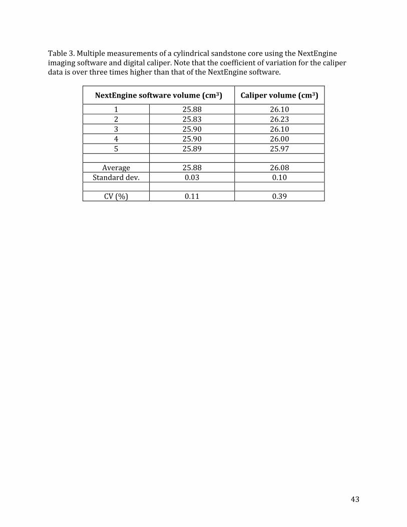
43

Table 3. Multiple measurements of a cylindrical sandstone core using the NextEngine imaging software and digital caliper. Note that the coefficient of variation for the caliper data is over three times higher than that of the NextEngine software.

NextEngine software volume (cm3) Caliper volume (cm3)

1 25.88 26.10 2 25.83 26.23 3 25.90 26.10 4 25.90 26.00 5 25.89 25.97

Average 25.88 26.08 Standard dev. 0.03 0.10

CV (%) 0.11 0.39

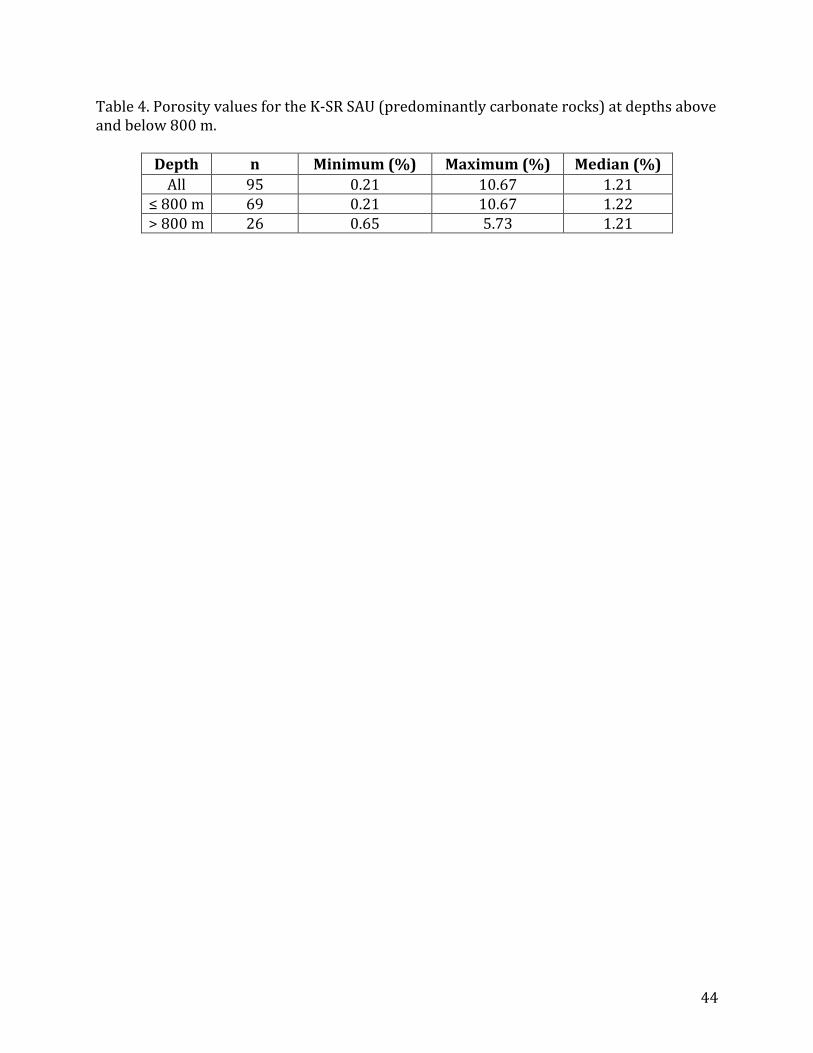
44

Table 4. Porosity values for the K-‐SR SAU (predominantly carbonate rocks) at depths above and below 800 m.

Depth n Minimum (%) Maximum (%) Median (%) All 95 0.21 10.67 1.21

≤ 800 m 69 0.21 10.67 1.22 > 800 m 26 0.65 5.73 1.21

45

Table 5. Porosity values by formation along with totals.

Formation ‡ n Minimum (%) Maximum (%) Median (%) Geometric Mean (%)† O -‐ Carters 7 0.60 4.91 0.99 1.20ABC O -‐ Lebanon 3 0.64 2.30 1.05 1.16ABC O -‐ Ridley 9 0.44 2.91 0.94 0.96BC O -‐ Murfreesboro 15 0.21 3.17 1.00 0.82C O – Wells Creek 6 1.02 6.29 1.47 2.10A O -‐ Mascot 20 0.44 10.67 1.44 1.85AB O -‐ Kingsport 10 0.98 6.50 1.33 1.89AB O -‐ Longview 4 0.63 1.24 1.20 1.03ABC O -‐ Chepultepec 6 0.89 1.61 1.16 1.15ABC Є – Copper Ridge 15 0.65 5.73 1.14 1.25ABC † Note: geomteric mean values with the same superscript letter are not significantly different at the 95% confidence level according to a protected t-‐test in SAS. ‡ Note: O: Ordovician, Є: Cambrian.

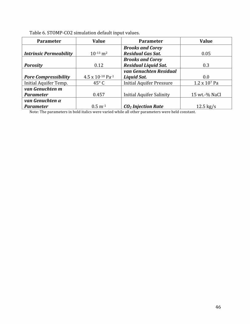
46

Table 6. STOMP-‐CO2 simulation default input values.

Note: The parameters in bold italics were varied while all other parameters were held constant.

Parameter Value Parameter Value

Intrinsic Permeability 10-‐13 m2 Brooks and Corey Residual Gas Sat. 0.05

Porosity 0.12 Brooks and Corey Residual Liquid Sat. 0.3

Pore Compressibility 4.5 x 10-‐10 Pa-‐1 van Genuchten Residual Liquid Sat. 0.0

Initial Aquifer Temp. 45° C Initial Aquifer Pressure 1.2 x 107 Pa van Genuchten m Parameter 0.457 Initial Aquifer Salinity 15 wt.-‐% NaCl van Genuchten α Parameter 0.5 m-‐1 CO2 Injection Rate 12.5 kg/s

47

Table 7. Parameter values, injection rates, volume of CO2 injected per year, and the resulting costs per metric ton of CO2.

Parameter Type

Parameter Value

Injection Rate (kg/s)

Volume of CO2 (metric tons/yr)

$/metric ton (2012 USD)

Intrinsic Permeability

(m2)

1.00 x 10-‐15 0.17 5447 $168.40 5.00 x 10-‐15 1.19 37391 $24.53 1.00 x 10-‐14 1.46 45980 $19.95 5.00 x 10-‐14 6.55 206447 $4.44 1.00 x 10-‐13 12.50 394200 $2.33 5.00 x 10-‐13 59.08 1863077 $0.49 1.00 x 10-‐12 119.20 3759011 $0.24

van Genuchten m paramter

0.426 11.56 364643 $2.52 0.438 11.93 376327 $2.44 0.457 12.50 394200 $2.33 0.516 14.33 452053 $2.03 0.537 14.68 462873 $1.98 0.547 15.07 475212 $1.93 0.556 15.27 481689 $1.90 0.600 16.34 515141 $1.78 0.672 17.79 561164 $1.63 0.696 18.17 572883 $1.60 0.708 18.32 577888 $1.59 0.772 19.21 605714 $1.52

Residual Gas Saturation

0.05 12.50 394200 $2.33 0.10 11.24 354442 $2.59 0.15 10.01 315587 $2.91 0.20 8.58 270627 $3.39 0.25 7.09 223595 $4.10 0.30 5.91 186356 $4.93

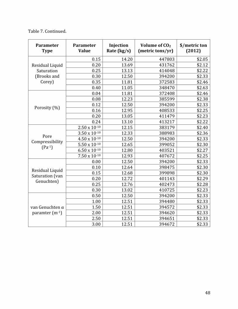
48

Table 7. Continued.

Parameter Type

Parameter Value


Volume of CO2 (metric tons/yr)

$/metric ton (2012)

Residual Liquid Saturation (Brooks and Corey)

0.15 14.20 447803 $2.05 0.20 13.69 431762 $2.12 0.25 13.13 414048 $2.22 0.30 12.50 394200 $2.33 0.35 11.81 372583 $2.46 0.40 11.05 348470 $2.63

Porosity (%)

0.04 11.81 372408 $2.46 0.08 12.23 385599 $2.38 0.12 12.50 394200 $2.33 0.16 12.95 408533 $2.25 0.20 13.05 411479 $2.23 0.24 13.10 413217 $2.22

Pore Compressibility

(Pa-‐1)

2.50 x 10-‐10 12.15 383179 $2.40 3.50 x 10-‐10 12.33 388983 $2.36 4.50 x 10-‐10 12.50 394200 $2.33 5.50 x 10-‐10 12.65 399052 $2.30 6.50 x 10-‐10 12.80 403521 $2.27 7.50 x 10-‐10 12.93 407672 $2.25

Residual Liquid Saturation (van Genuchten)

0.00 12.50 394200 $2.33 0.10 12.64 398475 $2.30 0.15 12.68 399898 $2.30 0.20 12.72 401143 $2.29 0.25 12.76 402473 $2.28 0.30 13.02 410725 $2.23

van Genuchten α paramter (m-‐1)

0.50 12.50 394200 $2.33 1.00 12.51 394480 $2.33 1.50 12.51 394572 $2.33 2.00 12.51 394620 $2.33 2.50 12.51 394651 $2.33 3.00 12.51 394672 $2.33

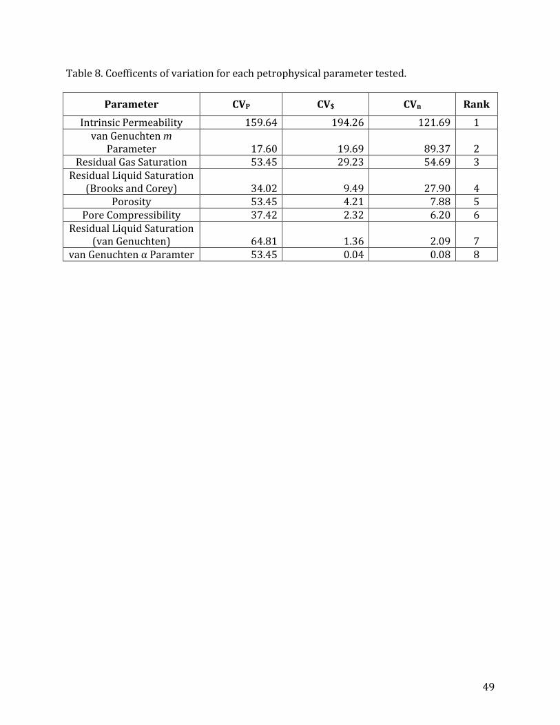
49

Table 8. Coefficents of variation for each petrophysical parameter tested.

Parameter CVP CV$ CVn Rank Intrinsic Permeability 159.64 194.26 121.69 1 van Genuchten m

Parameter 17.60 19.69 89.37 2 Residual Gas Saturation 53.45 29.23 54.69 3 Residual Liquid Saturation

(Brooks and Corey) 34.02 9.49 27.90 4 Porosity 53.45 4.21 7.88 5

Pore Compressibility 37.42 2.32 6.20 6 Residual Liquid Saturation

(van Genuchten) 64.81 1.36 2.09 7 van Genuchten α Paramter 53.45 0.04 0.08 8

50

Appendix 2. Figures

Figure 1. Stratigraphic column of the study area with units of interest highlighted (Gragg

and Perfect, 2011).

51

Figure 2. Four samples taken from the Exxon CU-‐30 core.

52

Figure 3. NextEngine Desktop 3D Scanner and scanned 3D image.

Core sample Scanner

Scanned Image

53

Figure 4. Porosity trend with depth for all cores.

0

200

400

600

800

1000

1200

1400

1600

1800 0.00 2.00 4.00 6.00 8.00 10.00 12.00

Depth (m

)

Porosity (%)

Stones River and Knox Groups SAU

54

Figure 5. Porosity trend with depth for the 4-‐44-‐309 basement test core (Smith County, Tennessee), covering both the Knox and Stones River groups.

0

200

400

600

800

1000

1200

1400

1600

1800 0.00 2.00 4.00 6.00 8.00 10.00 12.00

Depth (m

)

Porosity (%)

4-‐44-‐309

55

Figure 6. Porosity trend with depth for the Dupont geohydrological survey well core (Humphreys County, Tennessee), covering both the Knox and Stones River groups.

0

200

400

600

800

1000

1200

1400

1600

1800 0.00 2.00 4.00 6.00 8.00 10.00 12.00

Depth (m

)

Porosity (%)

Dupont

56

Figure 7. Porosity trends with depth for the 4-‐31-‐1 core (Davidson County, Tennessee), covering a portion of the Knox group, and the Exxon CU-‐30 core (Jackson County, Tennessee), covering most of the Stones River group. Note that these cores do not necessarily correlate to create a continuous stratigraphic sequence.

0

200

400

600

800

1000

1200

1400

1600

1800 0.00 2.00 4.00 6.00 8.00 10.00 12.00

Depth (m

)

Porosity (%)

4-‐31-‐1 and Exxon CU-‐30

4-‐31-‐1

CU-‐30

57

Figure 8. Porosity trends with depth for the 2-‐50-‐1 core (Overton County, Tennessee), covering portions of the Knox and Stones River groups, and the CA-‐5 core (Cannon, County, Tennessee), covering a portion of the Stones River group. Note that these cores do not necessarily correlate to create a continuous stratigraphic sequence.

0

200

400

600

800

1000

1200

1400

1600

1800 0.00 2.00 4.00 6.00 8.00 10.00 12.00

Depth (m

)

Porosity (%)

2-‐50-‐1 and CA-‐5

2-‐50-‐1

CA-‐5

58

Figure 9. Phase diagram for CO2 with red lines showing the default temperature, 45°C, and pressure, 1.2e7 Pa, for the model aquifer (modified from Bachu, 2000). Note that the default temperature and pressure values are adequate to maintain supercritical CO2.

59

Figure 10. A schematic visual representation of the model domain. One hundred grid cells were used with spacing increasing exponentially with distance from the injection well at the west border. Arrows indicate injected CO2. This model domain is based on a model created by Pruess et al. (2002).

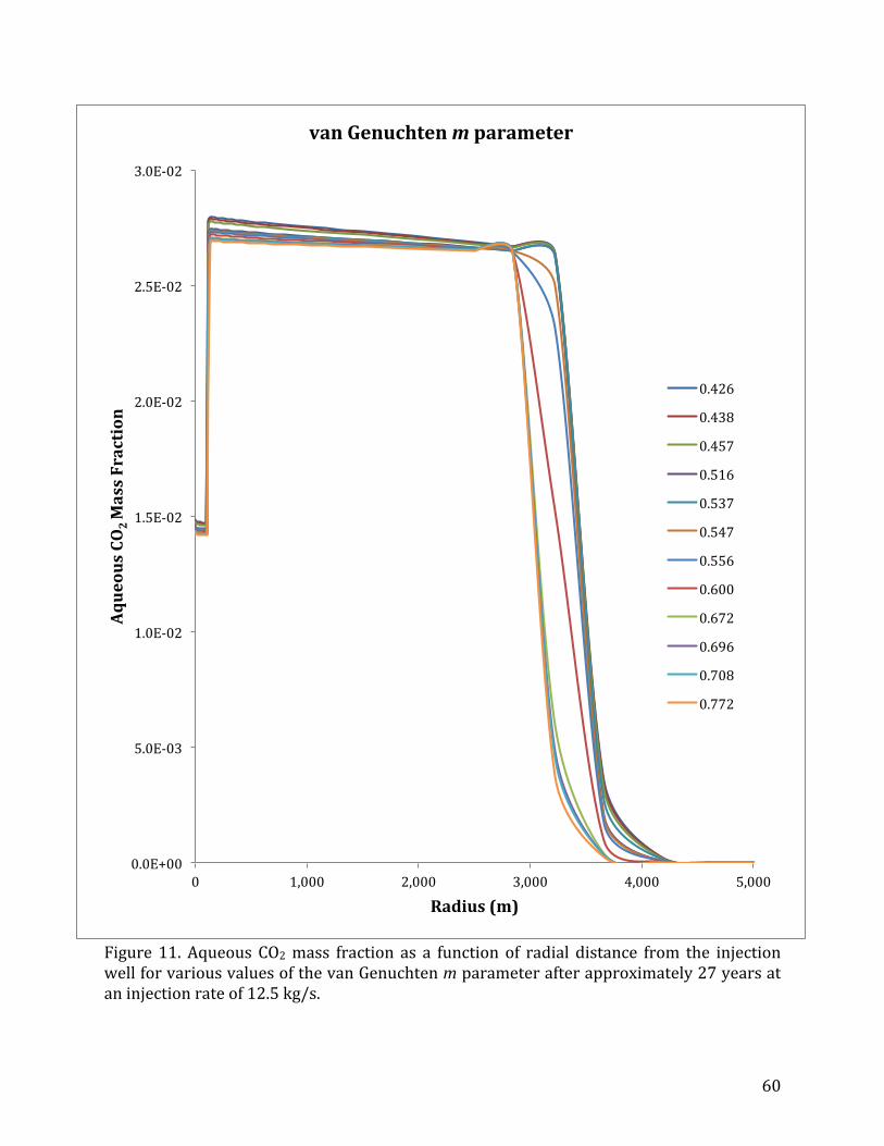
60

Figure 11. Aqueous CO2 mass fraction as a function of radial distance from the injection well for various values of the van Genuchten m parameter after approximately 27 years at an injection rate of 12.5 kg/s.

0.0E+00

5.0E-‐03

1.0E-‐02

1.5E-‐02

2.0E-‐02

2.5E-‐02

3.0E-‐02

0 1,000 2,000 3,000 4,000 5,000

Aqueous CO

2 Mass Fraction

Radius (m)

van Genuchten m parameter

0.426

0.438

0.457

0.516

0.537

0.547

0.556

0.600

0.672

0.696

0.708

0.772

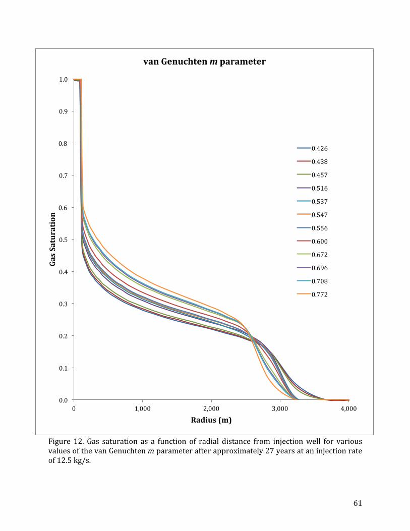
61

Figure 12. Gas saturation as a function of radial distance from injection well for various values of the van Genuchten m parameter after approximately 27 years at an injection rate of 12.5 kg/s.

0.0

0.1

0.2

0.3

0.4

0.5

0.6

0.7

0.8

0.9

1.0

0 1,000 2,000 3,000 4,000

Gas Saturation

Radius (m)


0.426

0.438

0.457

0.516

0.537

0.547

0.556

0.600

0.672

0.696

0.708

0.772

62

Figure 13. Gas pressure as a function of radial distance from injection well for various values of the van Genuchten m parameter after approximately 27 years at an injection rate of 12.5 kg/s.

1.00E+07

1.50E+07

2.00E+07

2.50E+07

3.00E+07

0 1,000 2,000 3,000 4,000 5,000

Gas Pressure (Pa)

Radius (m)


0.426

0.438

0.457

0.516

0.537

0.547

0.556

0.600

0.672

0.696

0.708

0.772

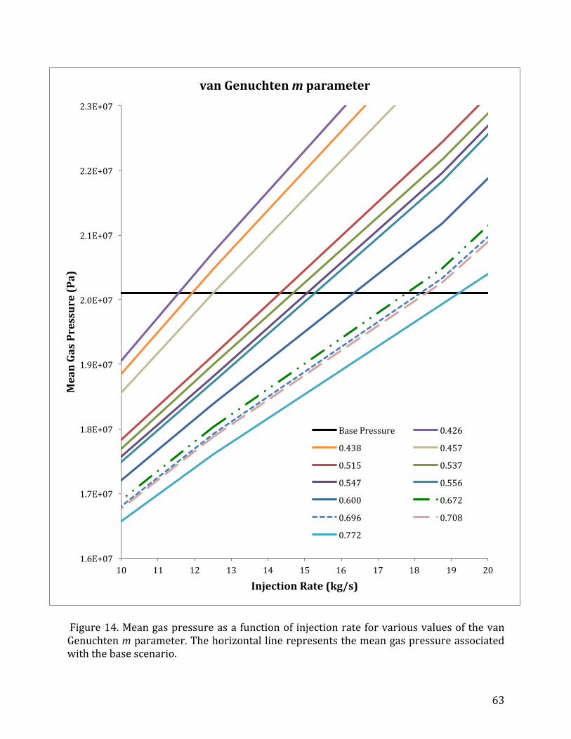
63

Figure 14. Mean gas pressure as a function of injection rate for various values of the van Genuchten m parameter. The horizontal line represents the mean gas pressure associated with the base scenario.

1.6E+07

1.7E+07

1.8E+07

1.9E+07

2.0E+07

2.1E+07

2.2E+07

2.3E+07

10 11 12 13 14 15 16 17 18 19 20

Mean Gas Pressure (Pa)



Base Pressure 0.426

0.438 0.457

0.515 0.537

0.547 0.556

0.600 0.672

0.696 0.708

0.772

64

Appendix 3. Raw Porosity Data

Sample ID Depth (ft) Depth (m) Formation Group Porosity 4-‐31-‐1-‐01 2197.0 669.6 Ok OЄK 0.98 4-‐31-‐1-‐02 2051.0 625.1 Ok OЄK 2.01 4-‐31-‐1-‐03 1898.0 578.5 Ok OЄK 5.32 4-‐31-‐1-‐04 1748.0 532.8 Oma OЄK 1.43 4-‐31-‐1-‐05 1603.3 488.7 Oma OЄK 3.12 4-‐31-‐1-‐06 1450.0 442.0 Oma OЄK 1.43 H 01 286.3 87.3 Oca OSR 4.91 H 02 361.3 110.1 Oca OSR 0.91 H 03 436.7 133.1 Olb OSR 2.30 H 04 513.0 156.4 Ord OSR 0.63 H 05 586.2 178.7 Ord OSR 2.91 H 06 661.4 201.6 Ord OSR 2.65 H 07 736.1 224.4 Ord OSR 1.21 H 08 813.0 247.8 Om OSR 0.39 H 09 886.7 270.3 Om OSR 0.21 H 11 1108.8 337.9 Owc OSR 1.54 H 12 1257.7 383.3 Oma OЄK 1.46 H 13 1408.0 429.2 Oma OЄK 10.67 H 14 1557.9 474.9 Oma OЄK 1.60 H 15 1708.0 520.6 Oma OЄK 2.77 H 16 1859.6 566.8 Oma OЄK 0.44 H 17 2007.7 611.9 Olv OЄK 1.24 H 18 2159.3 658.2 Olv OЄK 0.63 H 19 2308.4 703.6 Oche OЄK 1.15 H 20 2458.3 749.3 Oche OЄK 1.17 H 21 2607.8 794.9 Oche OЄK 1.61 H 22 2757.7 840.5 Єcr OЄK 1.21 H 23 2910.6 887.1 Єcr OЄK 1.29 H 24 3056.2 931.5 Єcr OЄK 1.21 H 25 3206.2 977.2 Єcr OЄK 1.50 H 26 3360.6 1024.3 Єcr OЄK 5.73 H 27 3508.7 1069.4 Єcr OЄK 0.76 H 28 3660.3 1115.6 Єcr OЄK 1.05 D 01 5562.4 1695.4 Єcr OЄK 1.12 D 02 5365.5 1635.4 Єcr OЄK 2.16 D 03 5180.5 1579.0 Єcr OЄK 0.95 D 04 5009.0 1526.7 Єcr OЄK 1.63 D 05 4859.0 1481.0 Єcr OЄK 1.14 D 06 4694.7 1430.9 Єcr OЄK 0.70

65

D 07 4552.0 1387.4 Єcr OЄK 0.65 D 08 4378.0 1334.4 Єcr OЄK 1.09 D 09 4199.3 1279.9 Oche OЄK 1.17 D 10 4052.0 1235.0 Oche OЄK 1.00 D 11 3898.8 1188.3 Oche OЄK 0.89 D 12 3750.3 1143.1 Olv OЄK 1.21 D 13 3598.1 1096.7 Olv OЄK 1.20 D 14 3449.1 1051.3 Ok OЄK 1.34 D 15 3301.0 1006.1 Ok OЄK 1.28 D 16 3149.5 960.0 Oma OЄK 2.20 D 17 3000.0 914.4 Oma OЄK 0.76 D 18 2845.7 867.4 Oma OЄK 1.31 D 19 2702.0 823.6 Oma OЄK 1.30 D 20 2406.6 733.5 Oma OЄK 4.55 D 21 2549.4 777.1 Oma OЄK 1.41 D 22 2250.5 686.0 Oma OЄK 1.01 D 23 2100.0 640.1 Oma OЄK 1.26 D 24 1951.4 594.8 Owc OSR 5.49 D 25 1875.5 571.7 Owc OSR 6.29 D 26 1800.8 548.9 Owc OSR 1.12 D 27 1728.5 526.8 Om OSR 1.02 D 28 1653.6 504.0 Om OSR 0.36 D 29 1571.0 478.8 Om OSR 0.31 D 30 1498.6 456.8 Om OSR 2.19 D 31 1421.2 433.2 Ord OSR 0.57 D 32 1350.0 411.5 Ord OSR 0.44 D 34 1196.2 364.6 Olb OSR 0.64 D 35 1141.8 348.0 Oca OSR 1.12 2-‐50-‐1-‐001 1441.5 439.4 Om OSR 1.31 2-‐50-‐1-‐002 1517.4 462.5 Owc OSR 1.40 2-‐50-‐1-‐003 1614.3 492.0 Oma OЄK 5.60 2-‐50-‐1-‐004 1721.0 524.6 Oma OЄK 5.32 2-‐50-‐1-‐005 1818.5 554.3 Oma OЄK 1.83 2-‐50-‐1-‐006 1918.5 584.8 Oma OЄK 0.92 2-‐50-‐1-‐007 2014.5 614.0 Ok OЄK 3.03 2-‐50-‐1-‐008 2105.6 641.8 Ok OЄK 1.02 2-‐50-‐1-‐009 2209.5 673.5 Ok OЄK 1.22 2-‐50-‐1-‐010 2304.0 702.3 Ok OЄK 1.33 2-‐50-‐1-‐011 2375.0 723.9 Ok OЄK 6.50 CU30-‐001 677.5 206.5 Oca OSR 0.60 CU30-‐002 778.0 237.1 Oca OSR 0.87 CU30-‐003 862.0 262.7 Olb OSR 1.05 CU30-‐004 981.4 299.1 Ord OSR 0.49

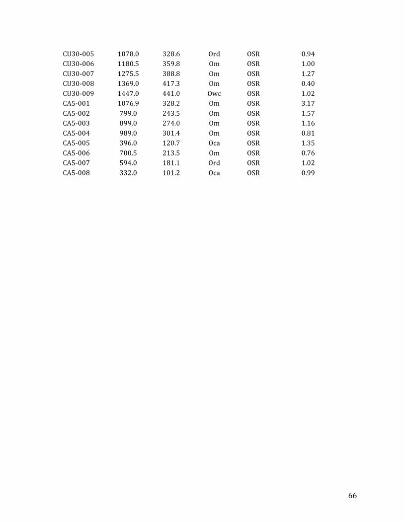
66

CU30-‐005 1078.0 328.6 Ord OSR 0.94 CU30-‐006 1180.5 359.8 Om OSR 1.00 CU30-‐007 1275.5 388.8 Om OSR 1.27 CU30-‐008 1369.0 417.3 Om OSR 0.40 CU30-‐009 1447.0 441.0 Owc OSR 1.02 CA5-‐001 1076.9 328.2 Om OSR 3.17 CA5-‐002 799.0 243.5 Om OSR 1.57 CA5-‐003 899.0 274.0 Om OSR 1.16 CA5-‐004 989.0 301.4 Om OSR 0.81 CA5-‐005 396.0 120.7 Oca OSR 1.35 CA5-‐006 700.5 213.5 Om OSR 0.76 CA5-‐007 594.0 181.1 Ord OSR 1.02 CA5-‐008 332.0 101.2 Oca OSR 0.99

67

Appendix 4. Example STOMP Input File 15 wt.-‐% Salinity Input File ~Simulation Title Card 1, Problem 3, M.D. White, Pacific Northwest Laboratory, 21 May 2002, 09:45 AM PST, 10, Intercomparison of simulation models for CO2 disposal in underground storage reservoirs. Test Problem 3: Radial Flow from a CO2 Injection Well This problem addresses two-‐phase flow of CO2 and water for simplified flow geometry and medium properties. The aquifer into which injection is made is assumed infinite-‐acting, homogeneous, and isotropic. Gravity and inertial effects are neglected, injection is made at a constant mass rate, and flow is assumed 1-‐D radial (line source). Under the conditions stated the problem has a similarity solution where dependence on radial distance R and time t occurs only through the similarity variable x = R2/t (O’Sullivan 1981; Doughty and Pruess 1992). ~Solution Control Card Normal, H2O-‐NaCl-‐CO2, 1, 0,day,1.e+5,day,1.e-‐3,s,1.e+4,day,1.15,16,1.e-‐06, 10000, Variable Aqueous Diffusion, Variable Gas Diffusion, 0, ~Grid Card Cylindrical, 100,1,1, 0.3,m,0.34068267,m,0.386882272,m,0.439346951,m,0.498926308,m,0.566585156,m, 0.643419145,m,0.730672508,m,0.829758203,m,0.9422808,m,1.070062462,m, 1.215172455,m,1.379960655,m,1.567095601,m,1.779607712,m,2.020938356,m, 2.294995583,m,2.606217409,m,2.959643684,m,3.360997708,m,3.81677891,m, 4.334368098,m,4.922146988,m,5.589633925,m,6.347638032,m,7.208434242,m, 8.185962079,m,9.296051391,m,10.55667869,m,11.98825828,m,13.61397279,m, 15.46014866,m,17.55668242,m,19.9375248,m,22.64123061,m,25.71158298,m, 29.19830246,m,33.15785213,m,37.65435198,m,42.76061723,m,48.55933748,m,

68

55.14441582,m,62.62248937,m,71.11465626,m,80.75843656,m,91.70999929,m, 104.1466914,m,118.2699096,m,134.308362,m,152.5217712,m,173.2050808,m, 196.6932312,m,223.3665839,m,253.6570806,m,288.0552382,m,327.1180922,m, 371.4782167,m,421.853969,m,479.0611216,m,544.0260733,m,617.8008506,m, 701.5801442,m,796.7206557,m,904.7630673,m,1027.456991,m,1166.789304,m, 1325.016317,m,1504.700323,m,1708.751078,m,1940.472932,m,2203.618331,m, 2502.448588,m,2841.802888,m,3227.176651,m,3664.810527,m,4161.79145,m, 4726.16741,m,5367.077773,m,6094.901285,m,6921.424143,m,7860.030856,m, 8925.920993,m,10136.35532,m,11510.93531,m,13071.92059,m,14844.58935,m, 16857.64778,m,19143.69485,m,21739.75025,m,24687.85387,m,28035.74657,m, 31837.64332,m,36155.1111,m,41058.06594,m,46625.90509,m,52948.79278,m, 60129.12031,m,68283.16417,m,77542.96894,m,88058.48564,m,100000,m,100000,m, 0.0,deg,45.0,deg, 0.0,m,100.0,m, ~Rock/Soil Zonation Card 1, Aquifer,1,100,1,1,1,1, ~Mechanical Properties Card Aquifer,2650,kg/m^3,0.12,0.12,Compressibility,4.5e-‐10,1/Pa,100.0,bar,Millington and Quirk, ~Hydraulic Properties Card Aquifer,1.0e-‐13,m^2,,,,,0.8,0.8, ~Saturation Function Card Aquifer,van Genuchten,0.5,1/m,1.84162,0.0,0.457,, ~Aqueous Relative Permeability Card Aquifer,Mualem Irreducible,0.457,0.30, ~Gas Relative Permeability Card Aquifer,Corey,0.05,0.30, ~Salt Transport Card Aquifer,0.0,m,0.0,m, ~Initial Conditions Card Gas Pressure,Aqueous Pressure, 4, Gas Pressure,120.0,Bar,,,,,,,1,100,1,1,1,1, Aqueous Pressure,120.0,Bar,,,,,,,1,100,1,1,1,1, Temperature,45.0,C,,,,,,,1,100,1,1,1,1, Salt Mass Fraction,0.15,,,,,,,,1,100,1,1,1,1,

69

~Source Card 1, Gas Mass Rate,Water-‐Vapor Mass Fraction,1,1,1,1,1,1,1, 0,s,120.0,bar,12.5,kg/s,0.0, ~Boundary Conditions Card 1, East,Aqu. Dirichlet,Gas Dirichlet,Aqu. Mass Frac., 100,100,1,1,1,1,1, 0,s,120.0,bar,0.0,120.0,bar,1.0,0.15,, ~Output Options Card 1, 64,1,1, 1,1,s,m,deg,6,6,6, 6, Gas Saturation,, Salt Saturation,, Salt Aqueous Mass Fraction,, CO2 Aqueous Mass Fraction,, Gas Pressure,Pa, Diffusive Porosity,, 4, 30,day, 100,day, 1000,day, 10000,day, 6, Gas Saturation,, Salt Saturation,, Salt Aqueous Mass Fraction,, CO2 Aqueous Mass Fraction,, Gas Pressure,Pa, Diffusive Porosity,,

70

Appendix 5. Supplimentary Figures

Aqueous CO2 mass fraction as a function of radial distance from the injection well for various values of intrinsic permeability after approximately 27 years at an injection rate of 12.5 kg/s.

0.0E+00

1.0E-‐02

2.0E-‐02

3.0E-‐02

4.0E-‐02

5.0E-‐02

6.0E-‐02

0 1,000 2,000 3,000 4,000 5,000 6,000

Aqueous CO

2 Mass Fraction

Radius (m)


1.00E-‐12 m^2

5.00E-‐13 m^2

1.00E-‐13 m^2

5.00E-‐14 m^2

1.00E-‐14 m^2

5.00E-‐15 m^2

1.00E-‐15 m^2

71

Gas saturation as a function of radial distance from injection well for various values of intrinsic permeability after approximately 27 years at an injection rate of 12.5 kg/s.

0.0

0.1

0.2

0.3

0.4

0.5

0.6

0.7

0.8

0.9

1.0

0 1,000 2,000 3,000 4,000 5,000 6,000

Gas Saturation

Radius (m)


1.00E-‐12 m^2

5.00E-‐13 m^2

1.00E-‐13 m^2

5.00E-‐14 m^2

1.00E-‐14 m^2

5.00E-‐15 m^2

1.00E-‐15 m^2

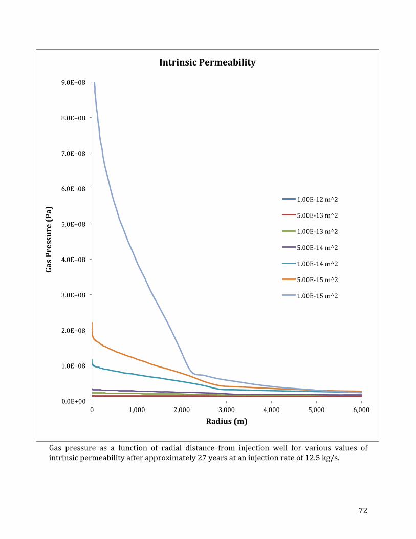
72

Gas pressure as a function of radial distance from injection well for various values of intrinsic permeability after approximately 27 years at an injection rate of 12.5 kg/s.

0.0E+00

1.0E+08

2.0E+08

3.0E+08

4.0E+08

5.0E+08

6.0E+08

7.0E+08

8.0E+08

9.0E+08

0 1,000 2,000 3,000 4,000 5,000 6,000

Gas Pressure (Pa)

Radius (m)


1.00E-‐12 m^2

5.00E-‐13 m^2

1.00E-‐13 m^2

5.00E-‐14 m^2

1.00E-‐14 m^2

5.00E-‐15 m^2

1.00E-‐15 m^2

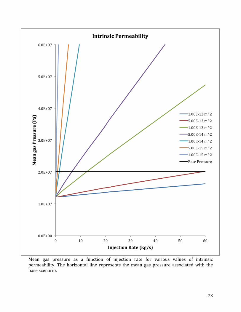
73

Mean gas pressure as a function of injection rate for various values of intrinsic permeability. The horizontal line represents the mean gas pressure associated with the base scenario.

0.0E+00

1.0E+07

2.0E+07

3.0E+07

4.0E+07

5.0E+07

6.0E+07

0 10 20 30 40 50 60

Mean gas Pressure (Pa)



1.00E-‐12 m^2

5.00E-‐13 m^2

1.00E-‐13 m^2

5.00E-‐14 m^2

1.00E-‐14 m^2

5.00E-‐15 m^2

1.00E-‐15 m^2

Base Pressure

74

Aqueous CO2 mass fraction as a function of radial distance from the injection well for various values of the Brooks and Corey residual gas saturation after approximately 27 years at an injection rate of 12.5 kg/s.

0.00E+00

5.00E-‐03

1.00E-‐02

1.50E-‐02

2.00E-‐02

2.50E-‐02

3.00E-‐02

3.50E-‐02

0 1,000 2,000 3,000 4,000 5,000 6,000

Aqueous CO

2 Mass Fraction

Radius (m)

Brooks and Corey Residual Gas Saturation

0.05

0.1

0.15

0.2

0.25

0.3

75

Gas saturation as a function of radial distance from injection well for various values of the Brooks and Corey residual gas saturation after approximately 27 years at an injection rate of 12.5 kg/s.

0.0

0.1

0.2

0.3

0.4

0.5

0.6

0.7

0.8

0.9

1.0

0 1,000 2,000 3,000 4,000 5,000 6,000

Gas Saturation

Radius (m)


0.05

0.1

0.15

0.2

0.25

0.3

76

Gas pressure as a function of radial distance from injection well for various values of the Brooks and Corey residual gas saturation after approximately 27 years at an injection rate of 12.5 kg/s.

1.4E+07

1.9E+07

2.4E+07

2.9E+07

3.4E+07

3.9E+07

0 1,000 2,000 3,000 4,000 5,000 6,000

Gas Pressure (Pa)

Radius (m)


0.05

0.1

0.15

0.2

0.25

0.3

77

Mean gas pressure as a function of injection rate for various values of the Brooks and Corey residual gas saturation. The horizontal line represents the mean gas pressure associated with the base scenario.

1.80E+07

1.85E+07

1.90E+07

1.95E+07

2.00E+07

2.05E+07

2.10E+07

2.15E+07

2.20E+07

2.25E+07

2.30E+07

3 5 7 9 11 13 15




0.05

0.1

0.15

0.2

0.25

0.3

Base Pressure

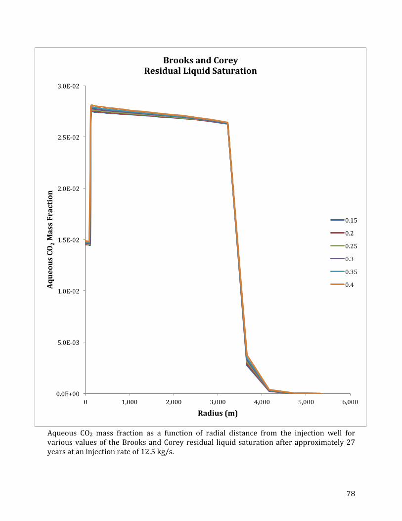
78

Aqueous CO2 mass fraction as a function of radial distance from the injection well for various values of the Brooks and Corey residual liquid saturation after approximately 27 years at an injection rate of 12.5 kg/s.

0.0E+00

5.0E-‐03

1.0E-‐02

1.5E-‐02

2.0E-‐02

2.5E-‐02

3.0E-‐02

0 1,000 2,000 3,000 4,000 5,000 6,000

Aqueous CO

2 Mass Fraction

Radius (m)

Brooks and Corey Residual Liquid Saturation

0.15

0.2

0.25

0.3

0.35

0.4

79

Gas saturation as a function of radial distance from injection well for various values of the Brooks and Corey residual liquid saturation after approximately 27 years at an injection rate of 12.5 kg/s.

0.0

0.1

0.2

0.3

0.4

0.5

0.6

0.7

0.8

0.9

1.0

0 1,000 2,000 3,000 4,000 5,000 6,000

Gas Saturation

Radius (m)


0.15

0.2

0.25

0.3

0.35

0.4

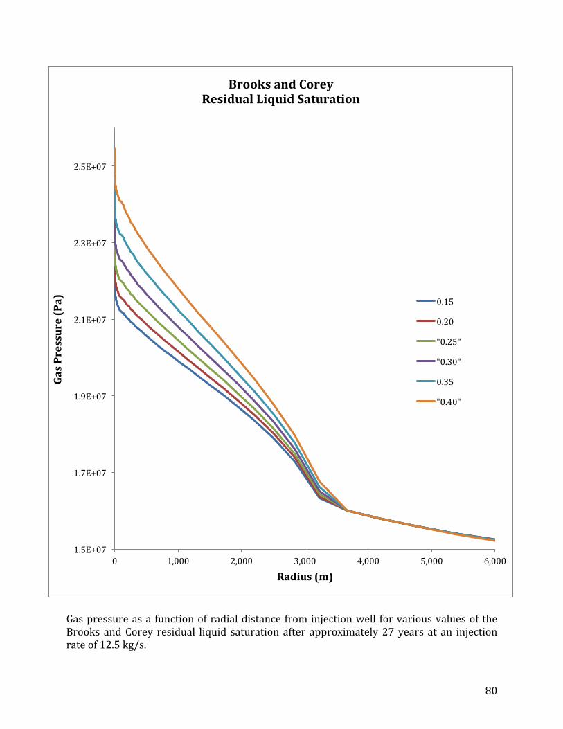
80

Gas pressure as a function of radial distance from injection well for various values of the Brooks and Corey residual liquid saturation after approximately 27 years at an injection rate of 12.5 kg/s.

1.5E+07

1.7E+07

1.9E+07

2.1E+07

2.3E+07

2.5E+07

0 1,000 2,000 3,000 4,000 5,000 6,000

Gas Pressure (Pa)

Radius (m)


0.15

0.20

"0.25"

"0.30"

0.35

"0.40"

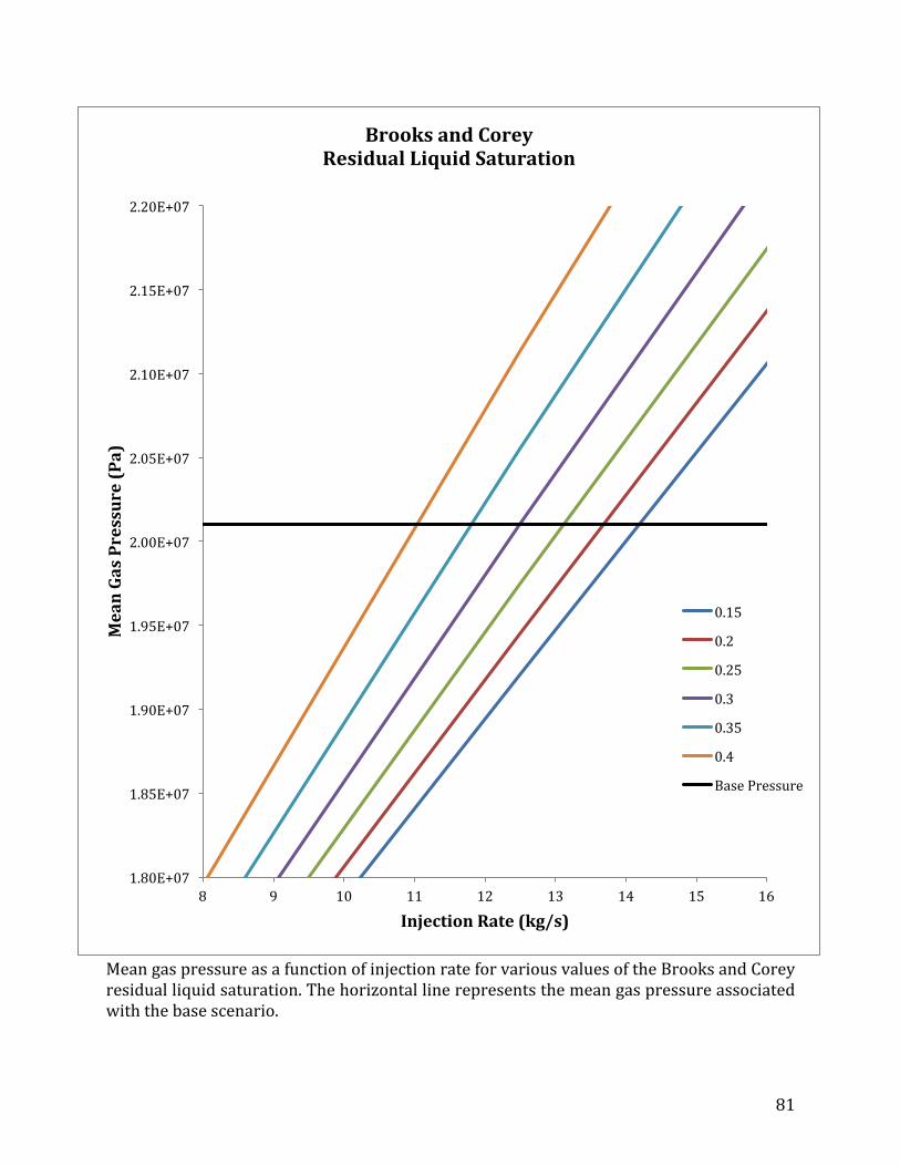
81

Mean gas pressure as a function of injection rate for various values of the Brooks and Corey residual liquid saturation. The horizontal line represents the mean gas pressure associated with the base scenario.

1.80E+07

1.85E+07

1.90E+07

1.95E+07

2.00E+07

2.05E+07

2.10E+07

2.15E+07

2.20E+07

8 9 10 11 12 13 14 15 16




0.15

0.2

0.25

0.3

0.35

0.4

Base Pressure

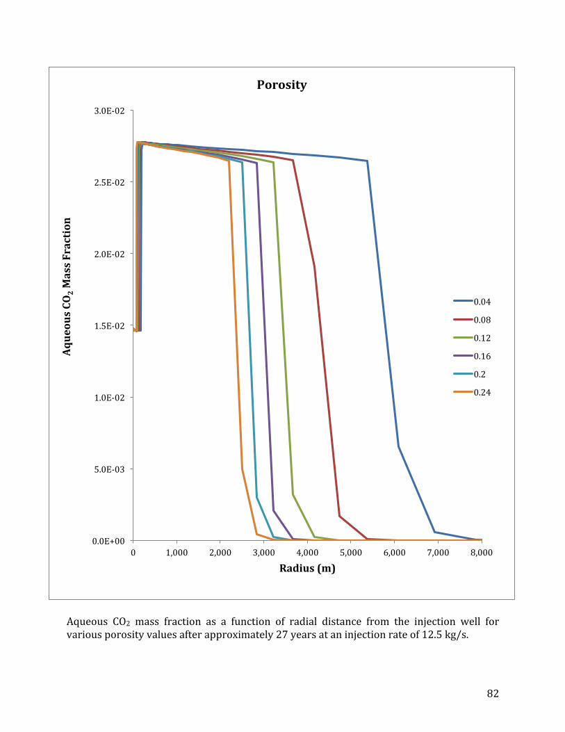
82

Aqueous CO2 mass fraction as a function of radial distance from the injection well for various porosity values after approximately 27 years at an injection rate of 12.5 kg/s.

0.0E+00

5.0E-‐03

1.0E-‐02

1.5E-‐02

2.0E-‐02

2.5E-‐02

3.0E-‐02

0 1,000 2,000 3,000 4,000 5,000 6,000 7,000 8,000

Aqueous CO

2 Mass Fraction

Radius (m)

Porosity

0.04

0.08

0.12

0.16

0.2

0.24

83

Gas saturation as a function of radial distance from injection well for various porosity values after approximately 27 years at an injection rate of 12.5 kg/s.

0.0

0.1

0.2

0.3

0.4

0.5

0.6

0.7

0.8

0.9

1.0

0 1,000 2,000 3,000 4,000 5,000 6,000 7,000 8,000

Gas Saturation

Radius (m)

Porosity

0.04

0.08

0.12

0.16

0.2

0.24

84

Gas pressure as a function of radial distance from injection well for various porosity values after approximately 27 years at an injection rate of 12.5 kg/s.

1.0E+07

1.2E+07

1.4E+07

1.6E+07

1.8E+07

2.0E+07

2.2E+07

2.4E+07

2.6E+07

0 1,000 2,000 3,000 4,000 5,000 6,000 7,000 8,000

Gas Pressure (Pa)

Radius (m)

Porosity

0.04

0.08

0.12

0.16

0.2

0.24

85

Mean gas pressure as a function of injection rate for various porosity values. The horizontal line represents the mean gas pressure associated with the base scenario.

1.90E+07

1.94E+07

1.98E+07

2.02E+07

2.06E+07

2.10E+07

11 11.5 12 12.5 13 13.5 14


Injection Rate (Kg/s)

Porosity

.04

.08

.12

.16

.20

.24

Base Pressure

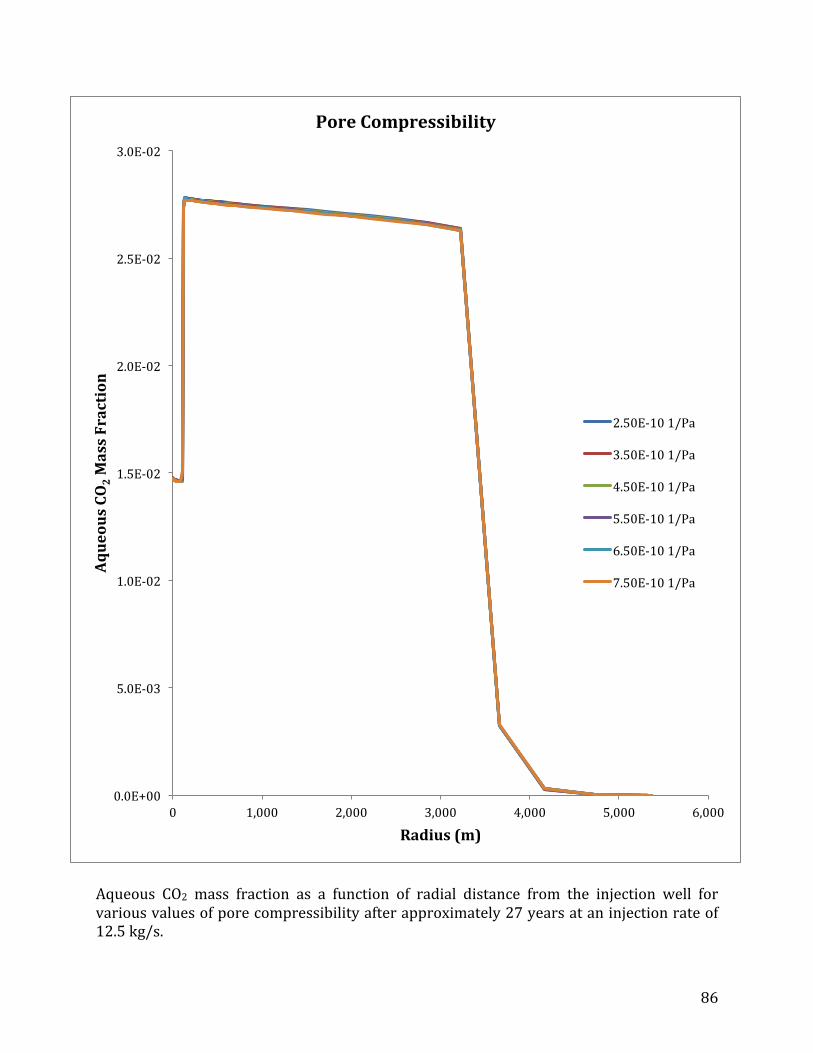
86

Aqueous CO2 mass fraction as a function of radial distance from the injection well for various values of pore compressibility after approximately 27 years at an injection rate of 12.5 kg/s.

0.0E+00

5.0E-‐03

1.0E-‐02

1.5E-‐02

2.0E-‐02

2.5E-‐02

3.0E-‐02

0 1,000 2,000 3,000 4,000 5,000 6,000

Aqueous CO

2 Mass Fraction

Radius (m)


2.50E-‐10 1/Pa

3.50E-‐10 1/Pa

4.50E-‐10 1/Pa

5.50E-‐10 1/Pa

6.50E-‐10 1/Pa

7.50E-‐10 1/Pa

87

Gas saturation as a function of radial distance from injection well for various values of pore compressibility after approximately 27 years at an injection rate of 12.5 kg/s.

0.0

0.1

0.2

0.3

0.4

0.5

0.6

0.7

0.8

0.9

1.0

0 1,000 2,000 3,000 4,000 5,000 6,000

Gas Saturation

Radius (m)


2.50E-‐10 1/Pa

3.50E-‐10 1/Pa

4.50E-‐10 1/Pa

5.50E-‐10 1/Pa

6.50E-‐10 1/Pa

7.50E-‐10 1/Pa

88

Gas pressure as a function of radial distance from injection well for various pore compressibility values after approximately 27 years at an injection rate of 12.5 kg/s.

1.4E+07

1.6E+07

1.8E+07

2.0E+07

2.2E+07

2.4E+07

2.6E+07

0 1,000 2,000 3,000 4,000 5,000 6,000

Gas Pressure (Pa)

Radius (m)


2.50E-‐10

3.50E-‐10

4.50E-‐10

5.50E-‐10

6.50E-‐10

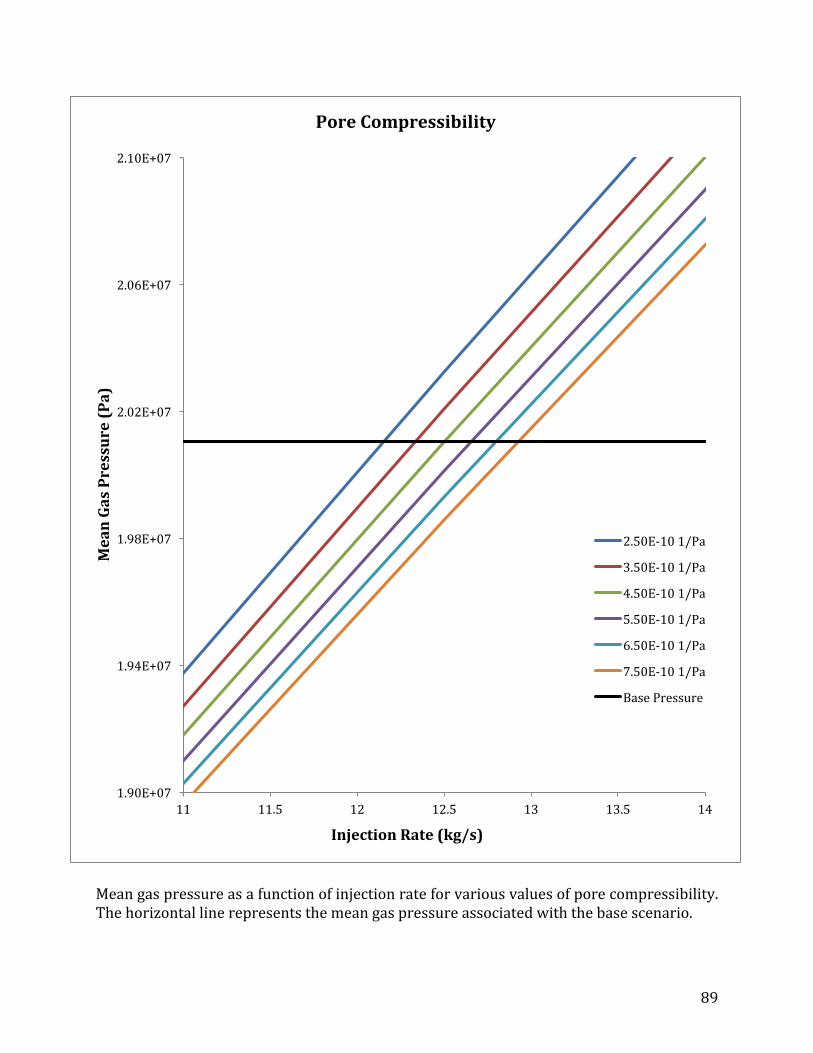
89

Mean gas pressure as a function of injection rate for various values of pore compressibility. The horizontal line represents the mean gas pressure associated with the base scenario.

1.90E+07

1.94E+07

1.98E+07

2.02E+07

2.06E+07

2.10E+07

11 11.5 12 12.5 13 13.5 14




2.50E-‐10 1/Pa

3.50E-‐10 1/Pa

4.50E-‐10 1/Pa

5.50E-‐10 1/Pa

6.50E-‐10 1/Pa

7.50E-‐10 1/Pa

Base Pressure

90

Aqueous CO2 mass fraction as a function of radial distance from the injection well for various values of the van Genuchten residual liquid saturation after approximately 27 years at an injection rate of 12.5 kg/s.

0.0E+00

5.0E-‐03

1.0E-‐02

1.5E-‐02

2.0E-‐02

2.5E-‐02

3.0E-‐02

0 1,000 2,000 3,000 4,000 5,000 6,000

Aque

ous C

O2 M

ass F

rac0on

Radius (m)

van Genuchten Residual Liquid Satura0on

0

0.1

0.15

0.2

0.25

0.3

91

Gas saturation as a function of radial distance from injection well for various values of the van Genuchten residual liquid saturation after approximately 27 years at an injection rate of 12.5 kg/s.

0.0

0.2

0.4

0.6

0.8

1.0

1.2

0 1,000 2,000 3,000 4,000 5,000 6,000

Gas Satura0

on

Radius (m)

van Genuchten Residual Liquid Satura0on

0

0.1

0.15

0.2

0.25

0.3

92

Gas pressure as a function of radial distance from injection well for various values of the van Genuchten residual liquid saturation after approximately 27 years at an injection rate of 12.5 kg/s.

1.5E+07

1.6E+07

1.7E+07

1.8E+07

1.9E+07

2.0E+07

2.1E+07

2.2E+07

2.3E+07

2.4E+07

0 1,000 2,000 3,000 4,000 5,000 6,000

Gas Pressure (Pa)

Radius (m)

van Genuchten Residual Liquid Saturation

0

0.10

0.15

0.20

0.25

0.30

93

Mean gas pressure as a function of injection rate for various values of the van Genuchten residual liquid saturation. The horizontal line represents the mean gas pressure associated with the base scenario.

1.95E+07

1.97E+07

1.99E+07

2.01E+07

2.03E+07

2.05E+07

12.2 12.3 12.4 12.5 12.6 12.7 12.8 12.9 13 13.1 13.2



van Genuchten Residual Liquid Saturation

0

0.1

0.15

0.2

0.25

0.3

Base Pressure

94

Aqueous CO2 mass fraction as a function of radial distance from the injection well for various values of the van Genuchten α parameter after approximately 27 years at an injection rate of 12.5 kg/s.

0.0E+00

5.0E-‐03

1.0E-‐02

1.5E-‐02

2.0E-‐02

2.5E-‐02

3.0E-‐02

0 1,000 2,000 3,000 4,000 5,000 6,000

Aqueous CO

2 Mass Fraction

Radius (m)

van Genuchten Alpha Parameter

0.5 1/m

1 1/m

1.5 1/m

2 1/m

2.5 1/m

3 1/m

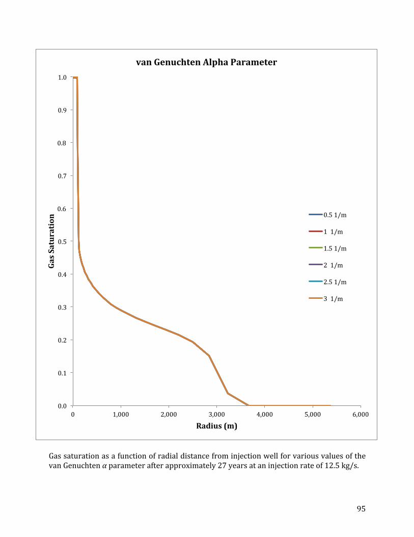
95

Gas saturation as a function of radial distance from injection well for various values of the van Genuchten α parameter after approximately 27 years at an injection rate of 12.5 kg/s.

0.0

0.1

0.2

0.3

0.4

0.5

0.6

0.7

0.8

0.9

1.0

0 1,000 2,000 3,000 4,000 5,000 6,000

Gas Saturation

Radius (m)


0.5 1/m

1 1/m

1.5 1/m

2 1/m

2.5 1/m

3 1/m

96

Gas pressure as a function of radial distance from injection well for various values of the van Genuchten α parameter after approximately 27 years at an injection rate of 12.5 kg/s.

1.4E+07

1.6E+07

1.8E+07

2.0E+07

2.2E+07

2.4E+07

2.6E+07

0 1,000 2,000 3,000 4,000 5,000 6,000

Gas Pressure

Radius (m)


0.5 1/m

1 1/m

1.5 1/m

2 1/m

2.5 1/m

3 1/m

97

Mean gas pressure as a function of injection rate for various values of the van Genuchten α parameter. The horizontal line represents the mean gas pressure associated with the base scenario.

2.354E+07

2.355E+07

2.356E+07

2.357E+07

12.48 12.49 12.50 12.51 12.52 12.53

Mean Gas pressure (Pa)



0.5 1/m

1 1/m

1.5 1/m

2 1/m

2.5 1/m

3 1/m

Base Pressure

98

Vita

Michael Gragg was born in Sandpoint, Idaho, to John and Elizabeth Gragg, and has

two younger brothers, Nickolus and Timothy. He attended several elementary schools but

graduated from East Bakersfield High School in Bakersfield, California. After graduation he

attended Bakersfield Community College, receiving his Associates of Arts degree in Liberal

Arts. He and his wife, Gretchen, and their first born son, Elijah, moved to Nashville,

Tennessee, where Michael attended and graduated Magna Cum Laude from Austin Peay

State University with a Bachelor’s of Science degree in geoscience with an emphasis in

geology. He and his family then moved to Knoxville, Tennessee, for graduate studies at the

University of Tennessee, Knoxville. Michael’s thesis topic was carbon sequestration in deep

saline aquifers and focused on porosity measurements, numerical modeling, and

fluctuations in costs associated with uncertainty of petrophysical parameters. Michael will

be graduating with is Master’s of Science in geology December of 2012 and plans to enter

the environmental consulting field.

CO2 Injection Into a Deep Saline Aquifer: Porosity ...

Documents

Transcript of CO2 Injection Into a Deep Saline Aquifer: Porosity ...