This draft manuscript is distributed solely for purposes of scientific peer review. Its content is deliberative and predecisional, so

it must not be disclosed or released by reviewers. Because the manuscript has not yet been approved for publication by the

U.S. Geological Survey (USGS), it does not represent any official USGS finding or policy.

Co-located contemporaneous mapping of morphological,

hydrological, chemical, and biological conditions in a 5th order

mountain stream network, Oregon, USA Adam S. Ward1, Jay P. Zarnetske2, Viktor Baranov3,4, Phillip J. Blaen5,6,7, Nicolai Brekenfeld5, Rosalie

Chu8, Romain Derelle9, Jennifer Drummond5,10, Jan Fleckenstein11,12, Vanessa Garayburu-Caruso13, 5

Emily Graham13, David Hannah5, Ciaran Harman14, Jase Hixson1, Julia L.A. Knapp15,16, Stefan Krause5,

Marie J. Kurz11,17, Jörg Lewandowski18,19, Angang Li20, Eugènia Martí10, Melinda Miller1, Alexander M.

Milner5, Kerry Neil1, Luisa Orsini9, Aaron I. Packman20, Stephen Plont2,21, Lupita Renteria22, Kevin

Roche23, Todd Royer1, Noah M. Schmadel1,24, Catalina Segura25, James Stegen13, Jason Toyoda8,

Jacqueline Wells22, Nathan I. Wisnoski26, Steven M. Wondzell27 10

1 O’Neill School of Public and Environmental Affairs, Indiana University, Bloomington, Indiana, USA 2 Department of Earth and Environmental Sciences, Michigan State University, East Lansing, Michigan, USA 3 LMU Munich Biocenter, Department of Biology II, Großhaderner Str. 2, 82152 Planegg-Martinsried, Germany 4 Department of River Ecology and Conservation, Senckenberg Research Institute and Natural History Museum, 63571 15 Gelnhausen, Germany 5 School of Geography, Earth & Environmental Sciences, University of Birmingham, Edgbaston. Birmingham. B15 2TT. UK 6 Birmingham Institute of Forest Research (BIFoR), University of Birmingham, Edgbaston. Birmingham. B15 2TT. UK 7 Yorkshire Water, Halifax Road, Bradford, BD6 2SZ 8 Environmental Molecular Sciences Laboratory, Pacific Northwest National Laboratory, Richland, WA, USA 20 9 Environmental Genomics Group, School of Biosciences, the University of Birmingham, Birmingham B15 2TT, UK 10 Integrative Freshwater Ecology Group, Centre for Advanced Studies of Blanes (CEAB-CSIC), Blanes, Spain 11 Dept. of Hydrogeology, Helmholtz Center for Environmental Research - UFZ, Permoserstraße 15, 04318 Leipzig, Germany 12 Bayreuth Center of Ecology and Environmental Research, University of Bayreuth, 95440 Bayreuth, Germany 13 Earth and Biological Sciences Division, Pacific Northwest National Laboratory, Richland, WA, USA 25 14 Department of Environmental Health and Engineering, Johns Hopkins University, Baltimore, Maryland, USA 15 Department of Environmental Systems Science, ETH Zürich, Zurich, Switzerland 16 Center for Applied Geoscience, University of Tübingen, Tübingen, Germany

2

17 The Academy of Natural Sciences of Drexel University, Philadelphia, Pennsylvania, USA 18 Leibniz-Institute of Freshwater Ecology and Inland Fisheries, Department Ecohydrology, Müggelseedamm 310, 12587

Berlin, Germany 19 Humboldt University Berlin, Geography Department, Rudower Chaussee 16, 12489 Berlin, Germany 20 Department of Civil and Environmental Engineering, Northwestern University, Evanston, Illinois, USA 5 21 Department of Biological Sciences, Virginia Polytechnic Institute and State University, Blacksburg, Virginia, USA 22 Pacific Northwest National Laboratory, Richland, WA, USA 23 Department of Civil & Environmental Engineering & Earth Sciences, University of Notre Dame, Notre Dame, IN 24 Earth Surface Processes Division, U.S. Geological Survey, Reston, Virginia, USA 25 Forest Engineering, Resources, and Management, Oregon State University Corvallis, OR, USA 10 26 Department of Biology, Indiana University, Bloomington, Indiana, USA 27USDAForestService,PacificNorthwestResearchStation,Corvallis,Oregon,USA.

Correspondence to: Adam S. Ward (adamward@indiana.edu)

15 Abstract. A comprehensive set of measurements and calculated metrics describing physical, chemical, and biological

conditions in the river corridor is presented. These data were collected in a catchment-wide, synoptic campaign in Lookout

Creek within the H.J. Andrews Experimental Forest (Cascade Mountains, Oregon, USA) in summer 2016 during low

discharge conditions. Extensive characterization of 62 sites including surface water, hyporheic water, and streambed

sediment was conducted spanning 1st through 5th order reaches in the river network. The objective of the sample design and 20 data acquisition was to generate a novel data set to support scaling of river corridor processes across varying flows and

morphologic forms present in a river network. The data are available at

http://www.hydroshare.org/resource/f4484e0703f743c696c2e1f209abb842 (Ward, 2019)

1 Introduction

River corridor science is the study of the exchange of water, solutes, particulate matter, energy, and biota between surface 25 and subsurface domains, collectively called river corridor exchange (e.g., Brunke and Gonser, 1997; Boulton et al., 1998;

Harvey and Gooseff, 2015; Tonina and Buffington, 2009; Krause et al., 2011, 2017). These beneficial functions are

primarily derived from the interactions between physical, chemical, and biological processes in the river corridor (e.g.,

McDonnell et al., 2007; Boano et al., 2014; Ward, 2015; Bernhardt et al., 2017). In a recent review, Ward (2015) identified

two key deficiencies that must be addressed to advance our predictive understanding of the functioning of the river corridor. 30 First, although the physical, chemical and biological processes are known to be tightly coupled and co-evolved, they are

3

seldom co-investigated. More comprehensive characterizations of physical-chemical-biological conditions are required to

enable the study of coupled processes that span these sub-systems. Second, most comprehensive, interdisciplinary studies are

conducted at single locations within an extensive river network and are limited in their range of spatial and temporal scales.

Combined, these limitations have hindered our predictive understanding of ecosystem services and functions at the scale of

river networks (Ward and Packman, 2018). While interactions between physical, chemical, and biological processes is 5 necessary to improve our predictive understanding at the scale of river networks, this knowledge is not sufficient to achieve

that goal.

In addition to local-scale understanding of process interactions and controls, predictive understanding of process dynamics in

river networks requires an understanding of spatial structure of processes and their interactions. Traditional studies of river 10 corridors focus on interpretation of time-series analysis of repeated at fixed points. However, an emerging class of data sets

and approaches emphasize the value of spatially distributed sampling campaigns in understanding the structure and function

of river corridors (e.g., Kaufmann et al. 1991; Wolock et al. 1997; Dent and Grimm, 1999; Temnerud & Bishop 2005; Likens et

al, 2006; Hale and Godsey, 2019). Spatially distributed studies along river corridors may provide increased information

about biogeochemical processes in comparison to equal effort in characterization of local-scale processes at a size (Lee-15 Cullin et al., 2018). Similarly, these data sets are driving innovation in the frameworks used to interpret spatially distributed

data sets, including foci on spatiotemporal variance (Abbott et al., 2018), the application of geostatistical approaches to

characterize scale-dependent relationships linking stream water chemistry and basin characteristics (Zimmer et al., 2013;

McGuire et al., 2014; Dupas et al., 2019); and additional spatial statistics methods (Isaak et al., 2014; Lowe et al., 2006).

20 While each of the studies cited above have made advances, they remain limited in two important dimensions. First, the

studies cited above primarily focus on spatial patterns in stream water chemistry with limited characterization of biological

and physical dimensions of the river corridor. Second, these studies are almost exclusively focused on measurements in the

surface water domain rather than explicitly considering hyporheic waters and the streambed sediments themselves.

Consequently, interpretations of causal mechanisms are limited by incomplete characterization and an emphasis on instream 25 water. we have a limited ability to predict river corridor processes and the associated ecosystem functions at the spatio-

temporal scales of river networks, where water resource managers and policymakers typically operate (Krause et al., 2011).

In response, we endeavored to collect river corridor data that directly address the two limitations by acquiring simultaneous,

multidisciplinary measurements distributed across a river network. The result is a novel river corridor data set documented

herein that presents new opportunities for exploring multi-scale, interacting river corridor patterns and processes. 30 Specifically, this paper presents the collection of a synoptic-in-time, distributed-in-space characterization of physical,

chemical, and biological conditions in the river corridor of the 5th order Lookout Creek stream network within the H.J.

Andrews Experimental Forest and Long Term Ecological Research site (Cascade Mountains, Oregon, USA).

4

2. Study location and campaign design

2.1 Study catchment

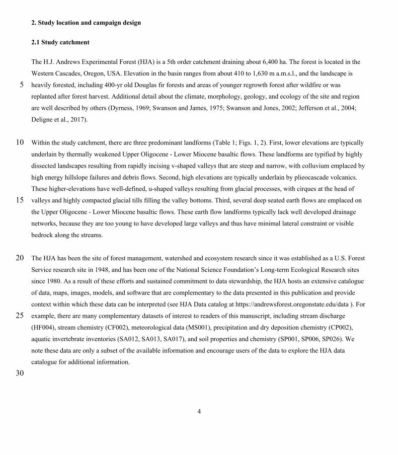
The H.J. Andrews Experimental Forest (HJA) is a 5th order catchment draining about 6,400 ha. The forest is located in the

Western Cascades, Oregon, USA. Elevation in the basin ranges from about 410 to 1,630 m a.m.s.l., and the landscape is

heavily forested, including 400-yr old Douglas fir forests and areas of younger regrowth forest after wildfire or was 5 replanted after forest harvest. Additional detail about the climate, morphology, geology, and ecology of the site and region

are well described by others (Dyrness, 1969; Swanson and James, 1975; Swanson and Jones, 2002; Jefferson et al., 2004;

Deligne et al., 2017).

Within the study catchment, there are three predominant landforms (Table 1; Figs. 1, 2). First, lower elevations are typically 10 underlain by thermally weakened Upper Oligocene - Lower Miocene basaltic flows. These landforms are typified by highly

dissected landscapes resulting from rapidly incising v-shaped valleys that are steep and narrow, with colluvium emplaced by

high energy hillslope failures and debris flows. Second, high elevations are typically underlain by plieocascade volcanics.

These higher-elevations have well-defined, u-shaped valleys resulting from glacial processes, with cirques at the head of

valleys and highly compacted glacial tills filling the valley bottoms. Third, several deep seated earth flows are emplaced on 15 the Upper Oligocene - Lower Miocene basaltic flows. These earth flow landforms typically lack well developed drainage

networks, because they are too young to have developed large valleys and thus have minimal lateral constraint or visible

bedrock along the streams.

The HJA has been the site of forest management, watershed and ecosystem research since it was established as a U.S. Forest 20 Service research site in 1948, and has been one of the National Science Foundation’s Long-term Ecological Research sites

since 1980. As a result of these efforts and sustained commitment to data stewardship, the HJA hosts an extensive catalogue

of data, maps, images, models, and software that are complementary to the data presented in this publication and provide

context within which these data can be interpreted (see HJA Data catalog at https://andrewsforest.oregonstate.edu/data ). For

example, there are many complementary datasets of interest to readers of this manuscript, including stream discharge 25 (HF004), stream chemistry (CF002), meteorological data (MS001), precipitation and dry deposition chemistry (CP002),

aquatic invertebrate inventories (SA012, SA013, SA017), and soil properties and chemistry (SP001, SP006, SP026). We

note these data are only a subset of the available information and encourage users of the data to explore the HJA data

catalogue for additional information.

30

5

2.2 Synoptic campaign design

This study was designed to replicate characterizations of the river corridor at a total of 62 sites spanning 1st through 5th

order reaches in the HJA. Site selection was based on (1) the presence of flowing surface waters; (2) stratification across

stream orders; (3) coverage of the three major landform units in the HJA; and (4) accessibility of sites. All sampling of water

and streambed sediment was conducted within the period 26-July through 3-Aug-2016 with no flow or precipitation events 5 recorded during the sampling campaign. All solute tracer experiments occurred during the period 31-July through 12-Aug-

2016, again with no recorded flow or precipitation events.

In addition to broad spatial coverage of the river network, we selected 4 subcatchments for a more detailed characterization

consisting of replication along the study reach at 4 to 6 locations per subcatchment. These 4 subcatchments were selected to 10 have one subcatchment in the 3 predominant landforms in the study catchment, plus a fourth subcatchment located where a

large debris flow scoured a section of the river corridor to bedrock in 1996 (Johnson, 2004). The objective of including 2

subcatchments in the low-elevation landform, was to provide a space-for-time comparison (i.e., WS01 and WS03 provide

two realizations of the same landform type at different states in response to the large debris flow that typifies a key geologic

disturbance in the system). 15

6

Figure 1. Synoptic sites and LiDAR-derived stream network (see details on network definition in section 3.1.1).

7

Figure 2. Headwater catchments in the major landform units at the H.J. Andrews Experimental Forest, including

multiple synoptic sites along an intensively studied reach. WS01 and WS03 are located in the Upper Oligocene-Lower

Miocene balsaltic flows, Unnamed Creek on a deep-seated earth flow, and Cold Creek in more modern Plieoscascade

volcanics. Characteristics of each landform and catchment are detailed in Table 1.

8

Table 1. Summary of site characteristics for the 4 headwater catchments where more intensive sampling was conducted. The

descriptions of these headwater catchments are considered representative of the major landform types within the HJA [after

Dyrness, 1969; Swanson and James, 1975; Swanson and Jones, 2002]. See catchment topography in Fig. 2 for each site.

5

Site Study Reach Geologic Setting Valley form Colluvium presence

and descriptionNotable river

corridor description Constraint Lateral Inflows Spatially Intermittant?

Lower

Middle

Upper

LowerDeposition of colluvium

from 1996 scouring event

Yes

MiddleIntermittant inceptisol-

based colluvium on bedrock

Isolated gravel wedges formed by large woody debris

Yes, below features

Upper Minimal colluvium present

100% Surface Flow (no colluvium) No

Upper

Lower

Upper Proportional to hillslope area

LowerAquifer extends

beyond catchment

Unknown at this time. Not expected

given apparent contributions from

aqufier.

Unknown at this time. Expected due

to the site of colluvial deposit.

Yes. Diurnal fluctuations in

stream discharge enable rapid shift

from continuous to intermittant over repeated 24-hr

cycles.

No known groundwater nor lateral inflows. Minimal lateral tributary area in

study reach

Cold

Cre

ek

Plieocascase volcanics atop Middle and Upper Miocene

Volcanics (Andesite, Basalt)

U-shaped valley (glacial cirque)

Compacted glacial tills

Large woody debris on till forms pools,

steps with intermediate

graveland cobble riffles

Bedrock visible at 1 location

Proportional to lateral tributary

area of hillslopes. Hillslopes

underlain by intact bedrock.

WS0

3 V-shaped valley w/ Narrow (2-10 m) valley bottom

Unna

med

Cre

ek Deep-seated earth failure on Upper

Oligocene - Lower Miocene Basaltic

Flows

Early downcutting & valley formation

in unstructure colluvial material

Extensive colluvium. Flat and wide valley bottom with lateral

meandering of active channel in incising

valley bottom

Meanders, cut banks more typical of alluvial valleys

compared to other study catchments

proposed

No visible bedrock in

active channel

WS0

1

Upper Oligocene - Lower Miocene Basaltic Flows,

Volcanoclastic Rocks. Thermally altered

(weakened) by subsequent volcanic

activity enabling rapid downcutting of the

valley bottoms.

V-shaped valley w/ Wide (10-20-m) valley bottom

Inceptisols. Abundant deposition from

hillslope debris flows. Highly porous.

Minimally compacted.

Pool-riffle-step and Pool-step-riffle

morphology. Channel splits. Gravel

wedges. Long, continuous sections of deposition from high-energy debris

flow events.

Observed lateral (valley

walls) and vertical

(streambed) constraint of

active channel

9

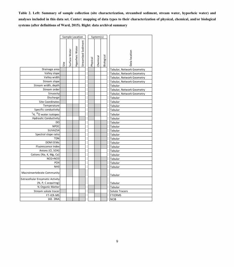
Table 2. Left: Summary of sample collection (site characterization, streambed sediment, stream water, hyporheic water) and

analyses included in this data set. Center: mapping of data types to their characterization of physical, chemical, and/or biological

systems (after definitions of Ward, 2015). Right: data archival summary

Site

Surf

ace

Wat

er

Hypo

rhei

c W

ater

Stre

ambe

d Se

dim

ent

Phys

ical

Chem

ical

Biol

ogic

al

Drainage area Tabular, Network GeometryValley slope Tabular, Network GeometryValley width Tabular, Network Geometry

Stream slope Tabular, Network GeometryStream width, depth Tabular

Stream order Tabular, Network GeometrySinuosity Tabular, Network Geometry

Discharge TabularSite Coordinates Tabular

Temperature TabularSpecific conductivity Tabular

2H, 18O water isotopes TabularHydraulic Conductivity Tabular

DO TabularNPOC Tabular

SUVA254 TabularSpectral slope ratio Tabular

TDN TabularDOM EEMs Tabular

Fluorescence Index TabularAnions (Cl, SO4) Tabular

Cations (Na, K, Mg, Ca) TabularNO2+NO3 Tabular

PO4 TabularNH3 Tabular

Macroinvertebrate CommunityTabular

Extracellular Enzymatic Activity (N, P, C acquiring) Tabular% Organic Matter Tabular

Stream solute tracer Solute TracersFT-ICR-MS FTICRMS

16S DNA NCIB

Sample Location System(s)

Data

loca

tion

10

3. Methods

3.1 Synoptic Site Characterization

3.1.1 Topographic Analysis

The stream network was derived from a 1-m digital terrain model based on airborne LiDAR collected in 2008 (Spies, 2018).

We used the one-directional flow accumulation algorithm (Seibert and McGlynn, 2007) implemented in a modified version 5 of TopoToolbox (Schwanghart and Kuhn, 2010; Schwanghart and Scherler, 2014) to derive the direction of flow and

accumulation of drainage area within the basin. We defined the stream network as any location draining more than 5 ha. The

threshold was established based on iteratively comparing the derived stream network to our experience working in headwater

catchments and their extent (consistent with analyses by Ward et al., 2018). The TopoToolbox algorithm defined study

reaches as the segment between two junctions. In our analysis, we defined 686 river corridor segments including a total 10 length of about 209 km of valley containing about 242 km of stream. For each study reach, we tabulated the sinuosity of the

stream within the valley. Next, we discretized each reach into 10-m segments, extracting valley slope, stream sinuosity, and

stream slope for each segment (after Corson-Rikert et al., 2016; Ward et al., 2018). Each synoptic site was assigned a stream

order and average valley slope, streambed slope, and sinuosity for the reach within which it was located.

15

3.1.2 Hydraulic and valley geometry

At each synoptic site, field observations of valley width were collected using a tape measure, with valley edge being visually

defined in the field based on the hillslope break-point between the relatively flat valley bottom and steeper valley walls.

Total wetted channel width was measured perpendicular to the direction of flow at the synoptic site, and average channel

depth was recorded based on at least five measurements of depth spaced evenly across the channel. 20

3.1.3 Hydraulic conductivity

At the approximate centerline of the synoptic site, a Solinst 615N drive-point piezometer (615N, Solinst Canada, Ltd.,

Georgetown, ON, Canada) was driven to a depth of about 65-cm below the streambed. The piezometer was screened over

the distance of 50-65-cm below the streambed. The piezometer was developed and purged by pumping slowly using a 25 peristaltic pump until the water was visually clear, typically about 5 minutes. Then hyporheic water sampling occurred as

described below (Section 3.2). Then a series of 3-6 replicates of a falling head test were conducted using the piezometer,

with water levels measured using a Van-Essen MicroDiver (DI601, Van Essen Instruments, Mukilteo, WA, USA),

recording at 0.5-s intervals and corrected for any variation in atmospheric pressure collecting data every 10-min. Falling

11

head data were used to estimate hydraulic conductivity after Hvorslev (1951). We report the geometric mean of the replicate

tests for each synoptic site. Finally, we note that at 5 sites there was minimal (~<10cm) to no colluvium present in the valley

bottom. At these sites we did not sample hyporheic water nor measure hydraulic conductivity, but we did collect streambed

sediment from small in-channel deposits at the synoptic site. These sites are necessary for complete representation of the

river corridor of the study catchment as there are many locations in the valley bottom that have minimal or no colluvium.. 5

3.1.4 Macroinvertebrate community

Benthic macroinvertebrate colonization pots were installed at 44 of the 62 synoptic sites using the design of Crossman et al.

(2012) during the synoptic campaign. Colonization pots were constructed of wire mesh with 1.25 cm openings formed into

cylinders approximately 15-cm in height and 8-cm in diameter, including a screened bottom. Hence, at sites where surface 10 sediment grain sizes were larger than 8-cm, they could not be installed. Substrate was excavated by hand and placed in each

pot prior to installing so that the top of each pot was level with the streambed. Colonization pots remained in situ for about 6

weeks following installation. Removal was achieved by pulling a cable to raise a specially constructed tarpaulin bag around

the sides of the pot before extraction, thereby minimizing sample loss. All substrate and macroinvertebrates were placed in a

90% ethanol solution for preservation. Additionally at 10 sites, surface samples of macroinvertebrates were collected with a 15 Surber sampler with a 330 micron mesh net, collected in triplicate at proximal locations and pooled for identification during

the synoptic campaign. Surface samples were processed using identical preservation methods; and identification was

conducted by the same researcher.

After separation of macroinvertebrates, sediment samples were oven dried and sieved to assemble grain size distributions for 20 each colonization pot. Importantly, because the pots were packed by hand in flowing water, we expect these grain size

distributions are biased toward the coarse fraction of streambed sediment, as finer materials would have washed away during

packing. Additionally, large cobbles would not have fit into the pots and excluded from collection.

Identification was performed under the stereomicroscope, except for the Chironomidae (family larvae and early larval instars 25 of the Plecoptera (order) and Ephemeroptera (order), which were mounted in the Euparal and examined under the light

microscope as described by Andersen (2013). Macroinvertebrates were identified to the lowest possible taxonomic level,

including the differentiation of adult and juvenile stages. Identification was performed using established keys (Merritt &

Cummins, 1996; Andersen, 2013; Malicky, 1983; Langton, 1991; Epler, 2001).

30

12

3.2 Water sampling & analyses

3.2.1 Sample collection from stream and hyporheic zone

All water samples were collected using a peristaltic pump to sample water at a flow rate of about 0.5 L/min. The pump

intake was located either in the stream thalweg for surface samples or in the developed piezometer for hyporheic samples.

Tubing was rinsed with water from the stream or hyporheic zone for at least 5 minutes prior to sample collection to minimize 5 cross-contamination between sites. We did not record the pumping rates nor volumes for this rinse, and acknowledge it may

have impact the flow field prior to sample collection. However, we expect this would be minimal because the sediment is

generally highly hydraulically conductive.

First, water temperature and dissolved oxygen were recorded using a YSI ProODO handheld probe (YSI, Inc., Yellow 10 Springs, OH, USA) with an optical dissolved oxygen (DO) sensor and thermistor. For stream samples, the probe was held in

the water column at the synoptic site near the pump intake.. For hyporheic samples, water was pumped into a small flow-

through cell until it overflowed, and then the sensor placed into cell while flow continued. For both stream and hyporheic

observations the sensor remained in place in the flowing water until probe readings for temperature and DO stabilized.

Specific conductivity was also measured with a handheld conductivity probe (YSI EC300; YSI, Inc., Yellow Springs, OH, 15 USA) using the same approaches.

Physical water samples for subsequent laboratory analyses were collected from the stream and hyporheic zone using

identical methods, including: (1) Unfiltered samples for water isotope analysis (Section 3.2.2) were collected in 20 mL glass

scintillation vials with conical inserts and were capped without headspace to minimize fractionation. (2) Samples for 20 dissolved water chemistry and nutrients (Section 3.2.3) were collected by field filtering using handheld 65 mL syringes.

Syringes were triple rinsed with sample water prior to collection of any sample volume. Samples for dissolved organic

carbon (DOC) analyses were field-filtered using a 0.2 μm cellulose acetate filter. Acid-washed amber HDPE bottles were

triple-rinsed with filtered sample water prior to sample collection. DOC samples were placed in a cooler with ice in the field

and remained chilled until analysis. Samples for dissolved nutrients, anions, and cations were field-filtered using a 0.45 μm 25 cellulose acetate filter. Sample bottles were triple-rinsed with filtered sample water prior to sample collection. Dissolved

nutrient samples were placed on dry ice in the field immediately after collection and remained frozen until analysis. (3)

Samples for microbial analysis (Section 3.2.4) were collected following Crevecoeur et al. (2015) by pumping water through

a Sterivex (Millipore) cartridge with a 0.22 μm Durapore (PVDF) filter membrane until either 1 L of water was filtered or 45

minutes elapsed. Cartridges were immediately sparged to remove site water, filled with RNAlater stabilization solution 30 (Ambion), and frozen in the field on dry ice. Samples remained frozen on dry ice until transferred and stored in a -80 °C

freezer until analysis.

13

3.2.2 Water stable isotopes ratios

We analyzed water stable isotopes to facilitate characterization of water ages using a cavity ring down spectroscopy method

(Picarro L2130-I, Picarro Inc.), following laboratory protocols described by Nickolas et al. (2017). Briefly, samples were run

under high-precision analysis mode using a 10 μL syringe for six injections per sample. We discarded the first three 5 injections to eliminate memory effects. We used internal standards to develop calibration equations for stable isotopes of

oxygen and hydrogen. The internal standards were calibrated using primary IAEA standards for Vienna Standard Mean

Ocean Water (VSMOW2: δ18O = 0.0‰, δ2H = 0.0‰), Standard Light Antarctic Precipitation (SLAP2: δ18O = −55.5‰, δ2H

= −427.5‰), and Greenland Ice Sheet Precipitation (GIPS: δ18O = −24.76‰, δ2H = −189.5‰). All stable isotopic values

were reported as delta (δ) values in parts per thousand (‰), which represent the deviation from the adopted VSMOW2 10 standard. Internal laboratory precision of the mean reported δ18O and δ2H values was estimated as 0.03‰ and 0.058‰ for

δ18O and δ2H respectively based on the analysis of >50 duplicate samples. The external accuracy - representing the overall

accuracy of the laboratory - was estimated as 0.058‰ and 0.241‰ for δ18O and δ2H by comparing >60 estimated values for

a known standard. A total of 7 samples collected for water isotope analysis were lost due to breakage of collection vials

during transport. Paired surface- and hyporheic samples were re-collected on 1-3 August 2016 for these locations. 15

3.2.3 Dissolved water chemistry and nutrients

Dissolved nutrients PO43-, NO2-+NO3-, and NH3 were analyzed on a San++ Automated Wet Chemistry Analyzer -

Segmented Flow Analyzer (Skalar Analytical B.V., Netherlands). Anions (Cl-, SO42-) and cations (Na+, K+, Mg2+, Ca2+) were

analyzed on a Dionex ICS5000 ion chromatography system (Thermo Fisher Scientific). Samples were thawed on the 20 laboratory bench prior to analysis (typically 2-4 hours) and were analyzed at room temperature.

DOC concentrations (as non-purgeable organic carbon, NPOC) and total dissolved nitrogen (TDN) were analyzed via acid-

catalyzed high temperature combustion using a Shimadzu TOC-L Analyzer with a TN module (Shimadzu Scientific

Instruments, Kyoto, Japan). Samples were allowed to come to room temperature prior to analysis. 25

Dissolved organic matter (DOM) optical quality was analyzed via absorbance and fluorescence spectroscopy. UV-visible

absorbance spectra ranging from 220 to 800 nm were collected using semi-micro, Brand-Tech cuvettes with a 1-cm path

length on a Shimadzu dual-beam UV 1800 spectrophotometer (Shimadzu Scientific Instruments, Kyoto, Japan). Samples

were allowed to come to room temperature prior to analyses. EPure water (18 MΩ, Barnstead EPure system) as a blank and 30 cuvettes were triplicate rinsed with Epure water and rinsed with sample water between readings.

14

Excitation-Emission Matrices (EEMs) were measured over excitation wavelengths of 250-450 nm and emission wavelengths

of 320-550 nm on a Horiba Aqualog Fluorometer (Horiba Scientific, Kyoto, Japan). Following the methods of Cory et al.

(2010b), EEMs were generated for each sample using a 4 second integration time using a quartz cuvette with a 1-cm path

length and Epure water as a blank. Samples were allowed to come to room temperature prior to analysis. Cuvettes were 5 rinsed with Epure water at least 10 times and triplicate rinsed with sample water between readings. EEMs were corrected for

instrument-specific excitation and emission corrections and the inner-filter effect (Cory et al., 2010b). Epure water blank

EEMs were collected and used to correct for Raman scattering. Fluorescence intensities from corrected-sample EEMs were

converted to Raman units (Stedmon and Bro, 2008). EEMs corrections and processing were performed using Matlab

consistent with Cory et al. (2010b). 10

Using EEMs and UV-visible absorbance spectra, several DOM quality indices were calculated for each sample. Specific UV

absorbance at 254 nm (SUVA254) was calculated using absorbance readings at 254 nm normalized for path length (in m-1)

and DOC concentration (in mg L-1). Higher SUVA254 values are associated with higher aromaticity of DOM (Weishaar et

al., 2003). Spectral slope ratio (SR) was calculated from absorbance spectra following the methods of Helms et al. (2008). 15 SR values correspond inversely to relative DOM molecular weight. Fluorescence Index (FI) was calculated following Cory

and McKnight (2005) as the ratio of emission (em) intensities for 470 nm and 520 nm at the 370 nm excitation (ex)

wavelength. FI values correspond to DOM source with lower FI values corresponding to allochthonous, terrestrially-derived

DOM and higher FI values corresponding to autochthonous, microbially-derived DOM (McKnight et al., 2001).

20 Intensities of specific EEMs peaks and absorbance wavelengths were selected and reported as well-documented proxies for

character and sources of DOM. Following Coble (1996) and Cory and Kaplan (2012), EEMs peak A (ex 250, 420/em 500)

and peak C (ex 250, 365/em 466) were reported as proxies for humic-like, terrestrially-derived fluorescent DOM (FDOM).

EEMs peak T (ex 250, 285/em 344) was reported as a proxy for protein-like FDOM (Cory and Kaplan, 2012). Specific

decadic and Naperian absorption coefficients reported serve as proxies for colored DOM (CDOM), and can be used as 25 indicators for specific sources and reactive fractions of the DOM pool (Spencer et al., 2009b). Decadic absorption

coefficients (in m-1) were calculated from absorbance readings at specific wavelengths normalized for path length (in m).

Naperian absorption coefficients (in m-1) are reported on a natural log scale and are calculated from absorbance readings at

specific wavelengths normalized for path length (in m) and multiplied by a factor of 2.303.

30

15

3.2.4 Microbial ecology

To characterize the bacterial communities collected from the surface water and hyporheic zone, we first isolated the filter

membrane from the Sterivex cartridge. We extracted DNA from the filters using the DNeasy PowerWater kit (Qiagen).

Following DNA extractions, we used PCR to amplify the V4-V5 region of the 16S rRNA gene using barcoded primers

(515F and 806R) designed for the Illumina MiSeq sequencing platform (Caporaso et al. 2012). The sequence libraries were 5 cleaned using the AMPure XP purification kit (Agencourt) and quantified using the PicoGreen dsDNA quantification kit

(Quant-iT, Invitrogen). Libraries were pooled at 10 ng per library. Pooled DNA and Total RNA libraries were sequenced on

the Illumina MiSeq platform at the Center for Genomics and Bioinformatics sequencing facility at Indiana University using

paired-end reads (Illumina Reagent Kit v2, 500-reaction kit).

10

3.3 Sediment sampling & analyses

3.3.1 Sample collection

Streambed sediment samples were collected near the piezometer at each synoptic site. Sample collection involved manually

removing the armor layer from the bed and then using a small specimen cup and putty knife to remove bed sediment without 15 loss of fines. Samples were sieved to remove coarse material using a 2-mm sieve. Sieved material was placed in a sterile 50-

mL centrifuge tube and frozen on dry ice immediately after collection. Samples were retained on dry ice or in a -80 °C

freezer until analysis. Duplicate sediment samples were collected for analysis of extracellular enzymatic activity at 9 sites.

Samples collected in this fashion were used for extracellular enzymatic activity and FT-ICR-MS analyses, detailed in

subsequent sections. 20

3.3.2 Extracellular Enzymatic Activity

Enzyme activities were determined using laboratory assays in which sediment extracts were exposed to model substrates that

are hydrolyzed by the enzymes (Table 3). Protocols were based on those described by Sinsabaugh et al. (1997) and Belanger

et al. (1997). Frozen sediment samples were thawed to room temperature and then 10 mL of 5-mM sodium bicarbonate 25 buffer solution was added to approximately 1 mL subsamples of sediment in 15-mL centrifuge tubes. These tubes were

homogenized with a vortex mixer for 15 s and then centrifuged for 15 min at 400 g. Samples were then stored in a

refrigerator overnight and the following day 200 µL of the supernatant was pipetted in triplicate onto 96-well microplates.

To ensure that any increase in fluorescence was due to enzyme activity, a set of control samples which had been boiled for 5

16

minutes to denature enzymes was also added to the plates. A set of standard solutions with known concentrations of

fluorescent product were also added to each plate to generate a standard curve.

Background fluorescence readings were recorded and substrate solution was added to start the enzyme reaction. Each well in

the microplate received 50 µL of a 200 µM substrate solution. Fluorescence measurements (440-nm emission intensity and 5 365-nm excitation wavelength) were recorded every ~30 min for at least 3 h. Microplates were protected from light and kept

at room temperature between readings. Fluorescence was measured using a BioTek Synergy Mx microplate reader. The

accumulation of fluorescent products (AMC or MUF, see Table 2) from the hydrolysis reactions was measured over time

and enzyme activity was calculated as the slope of a regression of AMC or MUF concentration against time.

10 About 1 mL of each sediment sample was dried, weighed, and then combusted at 550 oC and re-weighed to determine ash-

free dry mass (AFDM) and percent organic content for the sample (Wallace et al. 2006). Extracellular enzymatic activity

rates were then normalized to organic matter content and are reported in units of μmol g AFDM-1 h-1.

15

17

Table 3. Enzymes examined in this study and the reactions they catalyze.

Enzyme Model Substrate Product Reaction

β-D-glucosidase (GLU) 4-MUF-β-D-glucopyranoside

MUF1 Hydrolysis of glucose from cellobiose and cellulose

Alkaline phosphatase (AP) 4-MUF-phosphate MUF1 Hydrolysis of phosphate from phosphosaccarides and phospholipids

Leucine aminopeptidase (LAP)

L-Leucine -AMC AMC2 Hydrolysis of leucine from polypeptides

N-acetylglucosaminidase (NAG)

MUF-N-acetyl-β -D-glucosaminide

MUF1 Degradation of chitin and other β-1,4-linked glucosamine polymers

1 MUF = 4-methylumbelliferyl 2 AMC = 7-amino-4-methylcoumarin

3.3.3 Organic matter characterization 5

FT-ICR-MS solvent extraction and data acquisition

We performed Electrospray ionization (ESI) and Fourier transform ion cyclotron resonance (FT-ICR) mass spectrometry

(MS) using a 12 Tesla Bruker SolariX FT-ICR-MS located at the Environmental Molecular Sciences Laboratory (EMSL) in

Richland, WA, USA. Prior to mass spectrometry, organic matter was extracted from sediments by adding 1 ml of water

(18MΩ ionic purity) to 500 mg of sediments (after Tfaily et al. 2017). Each sediment sample was extracted 3x with the 10 above procedure. Supernatant from all extractions were combined and diluted to 5 mL to generate a final aliquot for analysis.

These aliquots were acidified to pH 2 with 85% phosphoric acid and extracted with PPL cartridges (Bond Elut), following

Dittmar et al. (2008). We performed weekly calibration after Tfaily et al. (2017) and instrument settings were optimized

using Suwannee River Fulvic Acid (IHSS). The instrument was flushed between samples using a mixture of water and

methanol. Blanks were analyzed at the beginning and the end of the day to monitor for background contaminants. 15

Samples were injected directly into the mass spectrometer and the ion accumulation time was set to 0.1s . Data were

collected from 98 – 900 m/z at 4M, yielding 144 scans that were co-added. A standard Bruker ESI source was used to

generate negatively charged molecular ions. Samples were introduced to the ESI source equipped with a fused silica tube (30

μm i.d.) through an Agilent 1200 series pump (Agilent Technologies) at a flow rate of 3.0 μL min-1. Experimental 20 conditions were as follows: needle voltage, +4.4 kV; Q1 set to 50 m/z; and the heated resistively coated glass capillary

operated at 180 °C.

18

FT-ICR-MS data processing

One hundred forty-four individual scans were averaged for each sample and internally calibrated using an organic matter

homologous series separated by 14 Da (–CH2 groups). The mass measurement accuracy was less than 1 ppm for singly

charged ions across a broad m/z range (100-1200 m/z). The mass resolution was ~240K at 341 m/z. The transient was 0.8

seconds. Data Analysis software (BrukerDaltonik version 4.2) was used to convert raw spectra to a list of m/z values 5 applying FTMS peak picker module with a signal-to-noise ratio (S/N) threshold set to 7 and absolute intensity threshold to

the default value of 100. Peaks were treated as presence/absence data because peak intensity differences are reflective of

ionization efficiency as well as relative abundance (Kujawinski and Behn, 2006; Minor et al., 2012; Tfaily et al., 2015;

Tfaily et al., 2017).

10 Putative chemical formulae were then assigned using in-house software following the Compound Identification Algorithm

(CIA), proposed by Kujawinski and Behn (2006), modified by Minor et al. (2012), and previously described in Tfaily et al.

(2017). Chemical formulae were assigned based on the following criteria: S/N >7, and mass measurement error <1 ppm,

taking into consideration the presence of C, H, O, N, S and P and excluding other elements. To ensure consistent formula

assignment, we aligned all sample peak lists for the entire dataset to each other in order to facilitate consistent peak 15 assignments and eliminate possible mass shifts that would impact formula assignment. We implemented the following rules

to further ensure consistent formula assignment: (1) we consistently picked the formula with the lowest error and with the

lowest number of heteroatoms and (2) the assignment of one phosphorus atom requires the presence of at least four oxygen

atoms.

20 The chemical character of thousands of peaks in each sample’s ESI FT-ICR-MS spectrum was evaluated on van Krevelen

diagrams. Compounds were plotted on the van Krevelen diagram on the basis of their molar H:C ratios (y-axis) and molar

O:C ratios (x-axis) (Kim et al., 2003). Van Krevelen diagrams provide a means to visualize and compare the average

properties of organic compounds and assign compounds to the major biochemical classes (e.g., lipid-, protein-, lignin-,

carbohydrate-, and condensed aromatic-like). In this study, biochemical compound classes are reported as relative abundance 25 values based on counts of C, H, and O for the following H:C and O:C ranges; lipids (0 < O:C ≤ 0.3, 1.5 ≤ H:C ≤ 2.5),

unsaturated hydrocarbons (0 ≤ O:C ≤ 0.125, 0.8 ≤ H:C < 2.5), proteins (0.3 < O:C ≤ 0.55, 1.5 ≤ H:C ≤ 2.3), amino sugars

(0.55 < O:C ≤ 0.7, 1.5 ≤ H:C ≤ 2.2), lignin (0.125 < O:C ≤ 0.65, 0.8 ≤ H:C < 1.5), tannins (0.65 < O:C ≤ 1.1, 0.8 ≤ H:C <

1.5), and condensed hydrocarbons (0 ≤ 200 O:C ≤ 0.95, 0.2 ≤ H:C < 0.8) (Tfaily et al., 2015).

30 Finally, we calculated the Gibbs Free Energy of OC oxidation under standard conditions (ΔGoCox) from the Nominal

Oxidation State of Carbon (NOSC) after La Rowe and Van Cappellen (2011). Though the exact calculation of ΔGoCox

necessitates an accurate quantification of all species involved in every chemical reaction in a sample, the use of NOSC as a

19

practical basis for determining ΔGoCox has been validated (Arndt et al., 2013; LaRowe and Van Cappellen, 2011; Graham

et al., 2017; Boye et al., 2017; Stegen et al., 2018).

3.4 Stream solute tracer

Two injections of a conservative solute tracer (NaCl) were conducted at 46 synoptic sites, one each at the upstream and

downstream reach boundaries to quantify discharge and short-term hyporheic flux. First, we fixed the upstream end of the 5 study reach at the same transect as the piezometer and sampling location. Next, we set the downstream station at a distance

of about 20 wetted channel widths downstream from the piezometer and sampling location, a length selected to capture a

representative valley segment (after Anderson et al., 2005). Minor variation in distance was allowed to place two specific

conductivity sensors in well-mixed locations within the stream channel, with the total length reported for each tracer study

reach. For each injection, mixing lengths for the solute tracer were visually estimated (after Payn et al., 2009; Ward et al., 10 2013b, 2013a), and small releases of a visual tracer were used to confirm mixing lengths when visual estimates were

uncertain. A known mass of NaCl was dissolved in stream water and released as an instantaneous injection one mixing

length upstream from the reach boundary. Initially, the downstream slug was released and measured only at the downstream

location to enable dilution gauging estimates of discharge at the downstream end of the study reach. Next, the upstream slug

was released and monitored at both locations to enable dilution gauging at the upstream transect, and evaluation of both 15 recovered and lost tracer along the study reach. The experimental design closely follows Payn et al. (2009) and Ward et al.

(2013b).

Solute tracer data at the reach boundaries were recorded as specific conductance (Onset Computer Corporation, Bourne,

MA, USA). We used a four point calibration curve constructed by dissolving known masses of NaCl in stream water to 20 convert specific conductance to salt concentration (C = 0.5022S; where C is NaCl concentration in mg/L and S is specific

conductance; r2 > 0.99). Notably, this equation does not include a y-intercept as we first subtracted background S from all

observations prior to conversion. In addition to providing the full solute tracer timeseries in the data set, we also provide

estimates of discharge (Q) based on dilution gauging, truncating the recovered tracer timeseries after 99% recovery (after

Mason et al., 2012; Ward et al., 2013b, 2013a). We report in the data set Q for both the upstream and downstream ends of 25 the study reach, and the change in Q along the study reach. Several additional metrics describing solute tracer timeseries are

detailed in Ward et al. (2019).

4. Data Availability

These data are archived in the Consortium of Universities for the Advancement of Hydrologic Science, Inc. (CUAHSI)

HydroShare data repository, accessible as http://www.hydroshare.org/resource/f4484e0703f743c696c2e1f209abb842 . In 30

20

addition to tabular data, timeseries for solute tracer experiments and detailed results from the FT-ICR-MS analyses are

archived. Raw sequence data for 16S DNA analyses are archived at the U.S. National Center for Biotechnology Information

(NCBI) as a BioProject (Accession: PRJNA534507 ).

5. Conclusions

We provide here a detailed characterization of physical, chemical, and biological parameters that are germane to the study of 5 river corridor exchange and associated ecosystem functions and services. These data represent state-of-the-science

characterization conducted at a heretofore unpresented resolution in space, and the only known data set that integrates across

physical, chemical, and biological dimensions of the river corridor, including coverage across 5 stream orders. Taken

together, these data will enable the testing of hypothesized processes and relationships in the river corridor across spatial

scales, and will be useful in the generation of testable hypotheses about river corridor exchanges in future studies. 10

Author Contributions.

All co-authors participated in the field collection, laboratory analysis, and/or curation of the data set. ASW was primarily

responsible for the writing of this manuscript and assembly of the archival database. ASW and JPZ conceived of the study

design with input from all co-authors. All authors contributed to the writing of this manuscript. 15

Competing Interests.

The authors report no conflicts of interest.

Acknowledgements

Funding for this research was provided by the Leverhulme Trust (Where rivers, groundwater and disciplines meet: a

hyporheic research network), the UK Natural Environment Research Council (Large woody debris – A river restoration 20 panacea for streambed nitrate attenuation? NERC NE/L003872/1), and the European Commission supported HiFreq: Smart

high-frequency environmental sensor networks for quantifying nonlinear hydrological process dynamics across spatial scales

(project ID 734317), the US Department of Energy (DOE) Office of Biological and Environmental Research (BER) as part

of Subsurface Biogeochemical Research Program’s Scientific Focus Area (SFA) at the Pacific Northwest National

Laboratory (PNNL). Data and facilities were provided by the HJ Andrews Experimental Forest and Long Term Ecological 25

21

Research program, administered cooperatively by the USDA Forest Service Pacific Northwest Research Station, Oregon

State University, and the Willamette National Forest and funded, in part, by the National Science Foundation under Grant

No. DEB-1440409. Ward’s time in preparation of this manuscript was supported by the University of Birmingham’s Institute

of Advanced Studies. Additional support to individual authors is acknowledged from National Science Foundation (NSF)

awards EAR 1652293, EAR 1417603, and EAR 1446328 and DOE award DE-SC0019377. Finally, the authors acknowledge 5 this would not have been possible without support from their home institutions.

References

Abbott, B. W., Gruau, G., Zarnetske, J. P., Moatar, F., Barbe, L., Thomas, Z., Fovet, O., Kolbe, T., Gu, S., Pierson-

Wickmann, A. C., Davy, P. and Pinay, G.: Unexpected spatial stability of water chemistry in headwater stream networks,

Ecol. Lett., 21(2), 296–308, doi:10.1111/ele.12897, 2018. 10 Anderson, J. K., Wondzell, S. M., Gooseff, M. N. and Haggerty, R.: Patterns in stream longitudinal profiles and implications

for hyporheic exchange flow at the H. J. Andrews Experimental Forest, Oregon, USA, Hydrol. Process., 19(15), 2931–2949,

2005.

Bailey, V. L., Smith, A. P., Tfaily, M., Fansler, S. J. and Bond-Lamberty, B.: Differences in soluble organic carbon

chemistry in pore waters sampled from different pore size domains, Soil Biol. Biochem., 107, 133–143, 15 doi:10.1016/j.soilbio.2016.11.025, 2017.

Belanger, C., Desrosiers, B. and Lee, K.: Microbial extracellular enzyme activity in marine sediments: extreme pH to

terminate reaction and sample storage, Aquat. Microb. Ecol., 13, 187–196 [online] Available from:

papers2://publication/uuid/C7916886-53F2-46B4-BAA5-547A62F8DA88, 1997.

Bernhardt, E. S., Blaszczak, J. R., Ficken, C. D., Fork, M. L., Kaiser, K. E. and Seybold, E. C.: Control Points in 20 Ecosystems: Moving Beyond the Hot Spot Hot Moment Concept, Ecosystems, 20(4), 665–682, doi:10.1007/s10021-016-

0103-y, 2017.

Boano, F., Harvey, J. W., Marion, A., Packman, A. I., Revelli, R., Ridolfi, L. and Worman, A.: Hyporheic flow and transport

processes: Mechanisms, models, and biogeochemical implications, Rev. Geophys., 52, 2012RG000417,

doi:10.1002/2012RG000417.Received, 2014. 25 Bolger, A. M., Lohse, M. and Usadel, B.: Trimmomatic: A flexible trimmer for Illumina sequence data, Bioinformatics,

30(15), 2114–2120, doi:10.1093/bioinformatics/btu170, 2014.

Boulton, A. J., Findlay, S., Marmonier, P., Stanley, E. H. and Valett, H. M.: The functional significance of the hyporheic

zone in streams and rivers, Annu. Rev. Ecol. Syst., 29(1), 59–81, 1998.

Boye, K., Noël, V., Tfaily, M. M., Bone, S. E., Williams, K. H., Bargar, J. R. and Fendorf, S.: Thermodynamically 30 controlled preservation of organic carbon in floodplains, Nat. Geosci., 10(6), 415–419, doi:10.1038/ngeo2940, 2017.

22

Breitling, R., Ritchie, S., Goodenowe, D., Stewart, M. L. and Barrett, M. P.: Ab initio prediction of metabolic networks

using Fourier transform mass spectrometry data, Metabolomics, 2(3), 155–164, doi:10.1007/s11306-006-0029-z, 2006.

Brunke, M. and Gonser, T.: The ecological significance of exchange processes between rivers and groundwater, Freshw.

Biol., 37, 1–33, 1997.

Coble, P. G.: Characterization of marine and terrestrial DOM in seawater using excitation-emission matrix spectroscopy, 5 Mar. Chem., 51(4), 325–346, doi:10.1016/0304-4203(95)00062-3, 1996.

Corson-Rikert, H. A., Wondzell, S. M., Haggerty, R. and Santelmann, M. V: Carbon dynamics in the hyporheic zone of a

headwater mountain streamin the Cascade Mountains, Oregon, Water Resour. Res., 52, 7556–7576,

doi:10.1029/2008WR006912.M, 2016.

Cory, R. M. and Kaplan, L. A.: Biological lability of streamwater fluorescent dissolved organic matter, Limnol. Oceanogr., 10 57(5), 1347–1360, doi:10.4319/lo.2012.57.5.1347, 2012.

Cory, R. M. and McKnight, D. M.: Fluorescence spectroscopy reveals ubiquitous presence of oxidized and reduced quinones

in dissolved organic matter, Environ. Sci. Technol., 39(21), 8142–8149, doi:10.1021/es0506962, 2005.

Cory, R. M., Miller, M. P., McKnight, D. M., Guerard, J. J. and Miller, P. L.: Effect of instrument-specific response on the

analysis of fulvic acid fluorescence spectra, Limnol. Oceanogr. Methods, 8(FEB), 67–78, doi:10.4319/lom.2010.8.67, 2010. 15 Crossman, J., Bradley, C., Milner, A. and Pinay, G.: INFLUENCE OF ENVIRONMENTAL INSTABILITY OF

GROUNDWATER‐FED STREAMS ON HYPORHEIC FAUNA, ON A GLACIAL FLOODPLAIN, DENALI NATIONAL

PARK, ALASKA, River Res. Appl., 29, 548–559, doi:10.1002/rra.1619, 2012.

Davids, M., Hugenholtz, F., Dos Santos, V. M., Smidt, H., Kleerebezem, M. and Schaap, P. J.: Functional profiling of

unfamiliar microbial communities using a validated de novo assembly metatranscriptome pipeline, PLoS One, 11(1), 1–19, 20 doi:10.1371/journal.pone.0146423, 2016.

Deligne, N. I., Mckay, D., Conrey, R. M., Grant, G. E., Johnson, E. R., O’Connor, J. and Sweeney, K.: Field-trip guide to

mafic volcanism of the Cascade Range in Central Oregon—A volcanic, tectonic, hydrologic, and geomorphic journey, Sci.

Investig. Rep., 110, doi:10.3133/sir20175022H, 2017.

Dent, C. L. and Grimm, N. B.: Spatial heterogeneity of stream water nutrient concentrations over successional time, 25 Ecology, 80(7), 2283–2298, doi:10.1890/0012-9658(1999)080[2283:SHOSWN]2.0.CO;2, 1999.

Dittmar, T., Koch, B., Hertkorn, N. and Kattner, G.: A simple and efficient method for the solid-phase extraction of

dissolved organic matter (SPE-DOM) from seawater, Limnol. Oceanogr. Methods, 6(6), 230–235,

doi:10.4319/lom.2008.6.230, 2008.

Dupas, R., Minaudo, C. and Abbott, B. W.: Stability of spatial patterns in water chemistry across temperate ecoregions, 30 Environ. Res. Lett., 14(7), 074015, doi:10.1088/1748-9326/ab24f4, 2019.

Dyrness, C. T.: Hydrologic properties of soils on three small watersheds in the western Cascades of Oregon, USDA For.

SERV RES NOTE PNW-111, SEP 1969. 17 P., 1969.

23

Epler, J. H. Identification manual for the larval Chironomidae (Diptera) of North and South Carolina. A guide to the

taxonomy of the midges of the southeastern United States, including Florida. Special Publication SJ2001-SP13. North

Carolina Department of Environment and Natural Resources, Raleigh, NC, and St. Johns River Water Management District,

Palatka, FL, 526. 2001.

Graham, E. B., Tfaily, M. M., Crump, A. R., Goldman, A. E., Bramer, L. M., Arntzen, E., Romero, E., Resch, C. T., 5 Kennedy, D. W. and Stegen, J. C.: Carbon Inputs From Riparian Vegetation Limit Oxidation of Physically Bound Organic

Carbon Via Biochemical and Thermodynamic Processes, J. Geophys. Res. Biogeosciences, 122(12), 3188–3205,

doi:10.1002/2017JG003967, 2017.

Haas, B. J., Papanicolaou, A., Yassour, M., Grabherr, M., Blood, P. D., Bowden, J., Couger, M. B., Eccles, D., Li, B.,

Lieber, M., Macmanes, M. D., Ott, M., Orvis, J., Pochet, N., Strozzi, F., Weeks, N., Westerman, R., William, T., Dewey, C. 10 N., Henschel, R., Leduc, R. D., Friedman, N. and Regev, A.: De novo transcript sequence reconstruction from RNA-seq

using the Trinity platform for reference generation and analysis, Nat. Protoc., 8(8), 1494–1512, doi:10.1038/nprot.2013.084,

2013.

Hale, R. L. and Godsey, S. E.: Dynamic stream network intermittence explains emergent dissolved organic carbon

chemostasis in headwaters, Hydrol. Process., 33(13), 1926–1936, doi:10.1002/hyp.13455, 2019. 15 Harvey, J. W. and Gooseff, M. N.: River corridor science: Hydrologic exchange and ecological consequences from bedforms

to basins, Water Resour. Res., Special Is, 1–30, doi:10.1002/2015WR017617.Received, 2015.

Helms, J. R., Stubbins, A., Ritchie, J. D., Minor, E. C., Kieher, D. J. and Mopper, K.: Absorption spectral slopes and slope

ratios as indicators of molecular weight, source, and photobleaching of chromophoric dissolved organic matter, Limnol.

Oceanogr., 53(3), 955–969, doi:10.1186/s12913-017-2639-8, 2008. 20 Hvorslev, M.J. Time lag and soil permeability in ground-water observations. Bulletin No. 36, Waterways Exper. Sta., Corps

of Engineers, U.S. Army, Vicksburg, Mississippi. 50 pp. 1951.

Isaak, D. J., Peterson, E. E., Ver Hoef, J. M., Wenger, S. J., Falke, J. A., Torgersen, C. E., Sowder, C., Steel, E. A., Fortin,

M.-J., Jordan, C. E., Ruesch, A. S., Som, N. and Monestiez, P.: Applications of spatial statistical network models to stream

data, Wiley Interdiscip. Rev. Water, 1(3), 277–294, doi:10.1002/wat2.1023, 2014. 25 Jefferson, A., Grant, G. E. and Lewis, S. L.: A River Runs Underneath It: Geological Control of Spring and Channel

Systems and Management Implications, Cascade Range, Oregon, in Advancing the Fundamental Sciences Proceedings of

the Forest Service: Proceedings of the Forest Service National Earth Sciences Conference, vol. 1, pp. 18–22., 2004.

Johnson, S. L.: Factors influencing stream temperatures in small streams: substrate effects and a shading experiment, Can. J.

Fish. Aquat. Sci., 61(6), 913–923, 2004. 30 Kaling, M., Schmidt, A., Moritz, F., Rosenkranz, M., Witting, M., Kasper, K., Janz, D., Schmitt-Kopplin, P., Schnitzler, J.-P.

and Polle, A.: Mycorrhiza-Triggered Transcriptomic and Metabolomic Networks Impinge on Herbivore Fitness, Plant

Physiol., 176(April), pp.01810.2017, doi:10.1104/pp.17.01810, 2018.

24

Kaufmann, P. R., Herlihy, A. T., Mitch, M. E., Messer, J. J. and Overton, W. S.: Stream chemistry in the eastern United

States: 1. Synoptic survey design, acid‐base status, and regional patterns, Water Resour. Res., 27(4), 611–627,

doi:10.1029/90WR02767, 1991.

Kim, S., Kramer, R. W. and Hatcher, P. G.: Graphical Method for Analysis of Ultrahigh-Resolution Broadband Mass

Spectra of Natural Organic Matter, the Van Krevelen Diagram, Anal. Chem., 75(20), 5336–5344, doi:10.1021/ac034415p, 5 2003.

Koch, B. P., Witt, M., Engbrodt, R., Dittmar, T. and Kattner, G.: Molecular formulae of marine and terrigenous dissolved

organic matter detected by electrospray ionization Fourier transform ion cyclotron resonance mass spectrometry, Geochim.

Cosmochim. Acta, 69(13), 3299–3308, doi:10.1016/j.gca.2005.02.027, 2005.

Krause, S., Hannah, D. M., Fleckenstein, J. H., Heppell, C. M., Kaeser, D. H., Pickup, R., Pinay, G., Robertson, A. L. and 10 Wood, P. J.: Inter‐disciplinary perspectives on processes in the hyporheic zone, Ecohydrology, 4(4), 481–499, 2011.

Krause, S., Lewandowski, J., Grimm, N. B., Hannah, D. M., Pinay, G., McDonald, K., Martí, E., Argerich, A., Pfister, L.,

Klaus, J., Battin, T., Larned, S. T., Schelker, J., Fleckenstein, J., Schmidt, C., Rivett, M. O., Watts, G., Sabater, F., Sorolla,

A. and Turk, V.: Ecohydrological interfaces as hot spots of ecosystem processes, Water Resour. Res., 53(8), 6359–6376,

doi:10.1002/2016WR019516, 2017. 15 Kujawinski, E. B. and Behn, M. D.: Automated analysis of electrospray ionization fourier transform ion cyclotron resonance

mass spectra of natural organic matter, Anal. Chem., 78(13), 4363–4373, doi:10.1021/ac0600306, 2006.

Langton, P. H. (1991). A key to pupal exuaviae of West Palaearctic Chironomidae. Langton.

Lee-Cullin, J. A., Zarnetske, J. P., Ruhala, S. S. and Plont, S.: Toward measuring biogeochemistry within the stream-

groundwater interface at the network scale: An initial assessment of two spatial sampling strategies, Limnol. Oceanogr. 20 Methods, 16(11), 722–733, doi:10.1002/lom3.10277, 2018.

Li, D., Liu, C. M., Luo, R., Sadakane, K. and Lam, T. W.: MEGAHIT: An ultra-fast single-node solution for large and

complex metagenomics assembly via succinct de Bruijn graph, Bioinformatics, 31(10), 1674–1676,

doi:10.1093/bioinformatics/btv033, 2015.

Likens, G. E. and Buso, D. C.: Variation in streamwater chemistry throughout the Hubbard Brook Valley, Biogeochemistry, 25 78(1), 1–30, doi:10.1007/s10533-005-2024-2, 2006.

Lowe, W. H., Likens, G. E. and Power, M. E.: Linking Scales in Stream Ecology, Bioscience, 56(7), 591, doi:10.1641/0006-

3568(2006)56[591:lsise]2.0.co;2, 2006.

Malicky, H. (1983). Atlas der europäischen Köcherfliegen (Vol. 24). Dr W Junk Publishing Company.

Mason, S. J. K., McGlynn, B. L. and Poole, G. C.: Hydrologic response to channel reconfiguration on Silver Bow Creek, 30 Montana, J. Hydrol., 438–439, 125–136, 2012.

McDonnell, J. J., Sivapalan, M., Vache, K., Dunn, S., Grant, G. E., Haggerty, R., Hinz, C., Hooper, R. P., Kirchner, J. and

Roderick, M. L.: Moving beyond heterogeneity and process complexity: A new vision for watershed hydrology, Water

Resour. Res., 43, W07301, 2007.

25

McGuire, K. J., Torgersen, C. E., Likens, G. E., Buso, D. C., Lowe, W. H. and Bailey, S. W.: Network analysis reveals

multiscale controls on streamwater chemistry, Proc. Natl. Acad. Sci. U. S. A., 111(19), 7030–7035,

doi:10.1073/pnas.1404820111, 2014.

McKnight, D. M., Boyer, E. W., Westerhoff, P. K., Doran, P. T., Kulbe, T. and Andersen, D. T.: Spectrofluorometric

characterization of dissolved organic matter for indication of precursor organic material and aromaticity, Limnol. Oceanogr., 5 46(1), 38–48, doi:10.4319/lo.2001.46.1.0038, 2001.

Merritt, R. W., & Cummins, K. W. (Eds.). An introduction to the aquatic insects of North America. Kendall Hunt

Publishing. 1996.

Minor, E. C., Steinbring, C. J., Longnecker, K. and Kujawinski, E. B.: Characterization of dissolved organic matter in Lake

Superior and its watershed using ultrahigh resolution mass spectrometry, Org. Geochem., 43, 1–11, 10 doi:10.1016/j.orggeochem.2011.11.007, 2012.

Moritz, F., Kaling, M., Schnitzler, J. P. and Schmitt-Kopplin, P.: Characterization of poplar metabotypes via mass difference

enrichment analysis, Plant Cell Environ., 40(7), 1057–1073, doi:10.1111/pce.12878, 2017.

Namiki, T., Hachiya, T., Tanaka, H. and Sakakibara, Y.: MetaVelvet: An extension of Velvet assembler to de novo

metagenome assembly from short sequence reads, Nucleic Acids Res., 40(20), doi:10.1093/nar/gks678, 2012. 15 Nickolas, L. B., Segura, C. and Brooks, J. R.: The influence of lithology on surface water sources, Hydrol. Process., 31(10),

1913–1925, doi:10.1002/hyp.11156, 2017.

Payn, R. A., Gooseff, M. N., McGlynn, B. L., Bencala, K. E. and Wondzell, S. M.: Channel water balance and exchange

with subsurface flow along a mountain headwater stream in Montana, United States, Water Resour. Res., 45, 2009.

Schwanghart, W. and Kuhn, N. J.: TopoToolbox: A set of Matlab functions for topographic analysis, Environ. Model. 20 Softw., 25(6), 770–781, doi:10.1016/j.envsoft.2009.12.002, 2010.

Schwanghart, W. and Scherler, D.: Short Communication: TopoToolbox 2 - MATLAB-based software for topographic

analysis and modeling in Earth surface sciences, Earth Surf. Dyn., 2(1), 1–7, doi:10.5194/esurf-2-1-2014, 2014.

Seibert, J. and McGlynn, B. L.: A new triangular multiple flow direction algorithm for computing upslope areas from

gridded digital elevation models, Water Resour. Res., 43(4), 1–8, doi:10.1029/2006WR005128, 2007. 25 Sinsabaugh, R. L., Findlay, S., Franchini, P. and Fischer, D.: Enzymatic analysis of riverine bacterioplankton production,

Limnol. Oceanogr., 42(1), 29–38, doi:10.4319/lo.1997.42.1.0029, 1997.

Spencer, R. G. M., Aiken, G. R., Butler, K. D., Dornblaser, M. M., Striegl, R. G. and Hernes, P. J.: Utilizing chromophoric

dissolved organic matter measurements to derive export and reactivity of dissolved organic carbon exported to the Arctic

Ocean: A case study of the Yukon River, Alaska, Geophys. Res. Lett., 36(6), 1–6, doi:10.1029/2008GL036831, 2009. 30 Spies, T. LiDAR Data (August 2008) for the Andrews Experimental Forest and Willamette National Forest Study Areas,

HJA Data Identifier GI010, Long-term Ecol. Res., For. Sci. Data Bank, Corvalliss, Oreg. (Database). (Available at

http://andlter.forestry.oregonstate.edu/data/abstract.aspx?dbcode=GI010 , Accessed 17 Jul. 2018). 2016.

26

Stedmon, C. A. and Bro, R.: Characterizing dissolved organic matter fluorescence with parallel factor analysis: A tutorial,

Limnol. Oceanogr. Methods, 6(11), 572–579, doi:10.4319/lom.2008.6.572, 2008.

Stegen, J. C., Johnson, T., Fredrickson, J. K., Wilkins, M. J., Konopka, A. E., Nelson, W. C., Arntzen, E. V., Chrisler, W. B.,

Chu, R. K., Fansler, S. J., Graham, E. B., Kennedy, D. W., Resch, C. T., Tfaily, M. and Zachara, J.: Influences of organic

carbon speciation on hyporheic corridor biogeochemistry and microbial ecology, Nat. Commun., 9(1), 1–11, 5 doi:10.1038/s41467-018-03572-7, 2018.

Swanson, F. J. and James, M. E.: Geology and geomorphology of the H.J. Andrews Experimental Forest, western Cascades,

Oregon, Portland, OR., 1975.

Swanson, F. J. and Jones, J. A.: Geomorphology and hydrology of the HJ Andrews experimental forest, Blue River, Oregon,

F. Guid. to Geol. Process. Cascadia, 36, 289–314, 2002. 10 Temnerud, J. and Bishop, K.: Spatial variation of streamwater chemistry in two Swedish boreal catchments: Implications for

environmental assessment, Environ. Sci. Technol., 39(6), 1463–1469, doi:10.1021/es040045q, 2005.

Tfaily, M. M., Podgorski, D. C., Corbett, J. E., Chanton, J. P. and Cooper, W. T.: Influence of acidification on the optical

properties and molecular composition of dissolved organic matter, Anal. Chim. Acta, 706(2), 261–267,

doi:10.1016/j.aca.2011.08.037, 2011. 15 Tfaily, M. M., Chu, R. K., Tolić, N., Roscioli, K. M., Anderton, C. R., Paša-Tolić, L., Robinson, E. W. and Hess, N. J.:

Advanced solvent based methods for molecular characterization of soil organic matter by high-resolution mass spectrometry,

Anal. Chem., 87(10), 5206–5215, doi:10.1021/acs.analchem.5b00116, 2015.

Tfaily, M. M., Chu, R. K., Toyoda, J., Tolić, N., Robinson, E. W., Paša-Tolić, L. and Hess, N. J.: Sequential extraction

protocol for organic matter from soils and sediments using high resolution mass spectrometry, Anal. Chim. Acta, 972, 54–20 61, doi:10.1016/j.aca.2017.03.031, 2017.

Tonina, D. and Buffington, J. M.: Hyporheic exchange in mountain rivers I: mechanics and environmental effects, Geogr.

Compass, 3(3), 1063–1086, doi:10.1111/j.1749-8198.2009.00226.x, 2009.

Tremblay, L. B., Dittmar, T., Marshall, A. G., Cooper, W. J. and Cooper, W. T.: Molecular characterization of dissolved

organic matter in a North Brazilian mangrove porewater and mangrove-fringed estuaries by ultrahigh resolution Fourier 25 Transform-Ion Cyclotron Resonance mass spectrometry and excitation/emission spectroscopy, Mar. Chem., 105(1–2), 15–

29, doi:10.1016/j.marchem.2006.12.015, 2007.

Wallace, JB, Hutchens, Jr., JJ, and Grubaugh, JW. Transport and storage of FPOM. Pages 249-271 in (FR Hauer and GA

Lamberti, editors) Methods in Stream Ecolgoy, 2nd Edition, Elsevier, New York. 2006.

Ward, A. S.: The evolution and state of interdisciplinary hyporheic research, Wiley Interdiscip. Rev. Water, 3(1), 83–103, 30 doi:10.1002/wat2.1120, 2015.

Ward, A.S., and A.I. Packman. Advancing our predictive understanding of river corridor exchange. WIREs: Water, 6(1),

e1327, 17pp, doi: 10.1002/wat2.1327 2019.

27

Ward, A. S., Gooseff, M. N., Voltz, T. J., Fitzgerald, M., Singha, K. and Zarnetske, J. P.: How does rapidly changing

discharge during storm events affect transient storage and channel water balance in a headwater mountain stream?, Water

Resour. Res., 49(9), 5473–5486, doi:10.1002/wrcr.20434, 2013a.

Ward, A. S., Payn, R. A., Gooseff, M. N., McGlynn, B. L., Bencala, K. E., Kelleher, C. A., Wondzell, S. M. and Wagener,

T.: Variations in surface water-ground water interactions along a headwater mountain stream: Comparisons between 5 transient storage and water balance analyses, Water Resour. Res., 49(6), 3359–3374, doi:10.1002/wrcr.20148, 2013b.

Ward, A. S., Schmadel, N. M. and Wondzell, S. M.: Simulation of dynamic expansion, contraction, and connectivity in a

mountain stream network, Adv. Water Resour., 114, 64–82, doi:10.1016/j.advwatres.2018.01.018, 2018.

Ward, A.S. ESSD, 2019 - Data Collection, HydroShare,

http://www.hydroshare.org/resource/f4484e0703f743c696c2e1f209abb842. 2019. 10 Ward, A. S., Wondzell, S. M., Schmadel, N. M., Herzog, S., Zarnetske, J. P., Baranov, V., Blaen, P. J., Brekenfeld, N., Chu,

R., Derelle, R., Drummond, J., Fleckenstein, J., Garayburu-Caruso, V., Graham, E., Hannah, D., Harman, C., Hixson, J.,

Knapp, J. L. A., Krause, S., Kurz, M. J., Lewendowski, J., Li, A., Marti, E., Miller, M., Milner, A. M., Neil, K., Orsini, L.,

Packman, A. I., Plont, S., Renteria, L., Roche, K., Royer, T., Segura, C., Stegen, J., Toyoda, J., Wells, J. and Wisnoski, N. I.:

Spatial and temporal variation in river corridor exchange across a 5th order mountain stream network, Hydrol. Earth Syst. 15 Sci. Discuss., (April), 1–39, doi:10.5194/hess-2019-108, 2019.

Wolock, D. M., Fan, J. and Lawrence, G. B.: Effects of basin size on low‐flow stream chemistry and subsurface contact time

in the Neversink River watershed, New York, Hydrol. Process., 11(9), 1273–1286, doi:10.1002/(sici)1099-

1085(199707)11:9<1273::aid-hyp557>3.3.co;2-j, 1997.

Zimmer, M. A., Bailey, S. W., Mcguire, K. J. and Bullen, T. D.: Fine scale variations of surface water chemistry in an 20 ephemeral to perennial drainage network, Hydrol. Process., 27(24), 3438–3451, doi:10.1002/hyp.9449, 2013.