Coevolving Communicative Behavior in a Linear Pursuer-Evader Game

Sevan G. Ficici, Jordan B. Pollack

DEMO Lab

Computer Science Department

Volen National Center for Complex Systems

Brandeis University

Waltham, MA

http://www.demo.cs.brandeis.edu

Abstract

The pursuer-evader (PE) game is recognized as an im-

portant domain in which to study the coevolution ofrobust adaptive behavior and protean behavior (Miller

and Cli�, 1994). Nevertheless, the potential of the

game is largely unrealized due to methodological hur-dles in coevolutionary simulation raised by PE; ver-

sions of the game that have optimal solutions (Isaacs,

1965) are closed-ended, while other formulations areopaque with respect to their solution space, for the

lack of a rigorous metric of agent behavior. This in-

ability to characterize behavior, in turn, obfuscates co-evolutionary dynamics. We present a new formulation

of PE that a�ords a rigorous measure of agent behav-

ior and system dynamics. The game is moved fromthe two-dimensional plane to the one-dimensional bit-

string; at each time step, the evader generates a bit

that the pursuer must simultaneously predict. Becausebehavior is expressed as a time series, we can employ

information theory to provide quantitative analysis of

agent activity. Further, this version of PE opens vis-tas onto the communicative component of pursuit and

evasion behavior, providing an open-ended serial com-

munications channel and an open world (via coevolu-

tion). Results show that subtle changes to our game

determine whether it is open-ended, and profoundly

a�ect the viability of arms-race dynamics.

1. Introduction

The pursuer-evader (PE) game is argued to be an impor-tant domain for coevolutionary simulation (Miller andCli�, 1994) due not only to its ubiquity in nature, butalso because it provides a parsimonious, yet powerful,framework of investigation: robust adaptive behavior,open-ended coevolution, and adaptively unpredictable,or protean, behavior all fall within its purview. In par-ticular, the PE game is believed to be rich enough tosupport the evolution of sophisticated perception, con-trol, and predictive ability; insight gained by evolvingagents for the game may impact disciplines in the biolog-ical and ethological communities. Nevertheless, the PEgame also presents methodological hurdles that highlight

shortcomings in the state of the art of coevolutionarysimulation itself. While some of these hurdles have dimin-ished, most notably the red-queen e�ect (Cli� and Miller,1995), many others remain that demand a more lucidunderstanding of coevolutionary learning. Key issues in-volve the conditions that instigate competitive arms races

or, to the contrary, mediocre stable-states (MSS) (Ange-line and Pollack, 1994; Pollack et al., 1997), neither ofwhich are well understood.

We posit that the spatially-oriented PE game bringsat least three di�culties to coevolutionary research: 1)the lack of a canonical form, which leads to 2) the ques-tion of open-endedness, and 3) the lack of a rigorous met-ric of agent behavior. First, there exist many versions ofthe PE game. The earliest formulations (Isaacs, 1965) aregames of perfect information where optimal pursuit andevasion strategies follow analytically from agent capabil-ities. More recent work casts PE into a purely discrete,non-kinematic reactive game (Koza, 1992; Reynolds,1994), or into a continuous game of, essentially, imperfectinformation that incorporates a two-dimensional physi-cal model (Cli� and Miller, 1996), for example. Second,these di�erences in game formulation impact the natureof the solution space; where PE formulations have opti-mal solutions, the game is closed-ended and, therefore,categorically less interesting than an open-ended domain.Further, these optimal solutions are not compelling ex-amples of evolved complexity; a formulation where op-timal pursuit is de�ned simply by reactively moving di-rectly towards the evader does not even require the pur-suer to hold state. Third, and �nally, agent behavior inPE is currently described exclusively in subjective, qual-itative terms; as (Cli� and Miller, 1996) point out, theredoes not yet exist a quantitative, operational measure bywhich one can characterize and judge agent behavior.

The hypothesized potential of the PE game is thuslargely unrealized due to the opaqueness of the do-main, of coevolutionary dynamics, and their interaction;we present a reformulation of the pursuer-evader gamethat helps clarify all three. Simply, we move the arena

of action from the two-dimensional plane to the one-dimensional bitstring; at each time step, the evader gen-erates a binary symbol that the pursuer must simulta-neously predict. Games last one thousand time steps. Atally of correct guesses is used to derive players' scores.Because behavior is expressed as a binary time series wecan take advantage of information theory to provide pre-cise characterizations of agent behavior and evolutionaryprogress.

As importantly, recasting the PE game in this wayopens vistas onto the communicative component of pur-suit and evasion behavior. Recent work by (Di Paolo,1997) raises a concern that much research on communi-cation con ates functional utility with operational pro-cess: the utility of communicative behavior may very wellbe that it confers adaptiveness, yet communication sode�ned fails utterly to describe the behavior itself. Sim-ilarly, the denotative function of `information' is oftencon ated with the process that generates it. In our PEgame we can characterize pursuit and evasion behavioroutside of the context of selective advantage. Further,we operationalize the behaviors and unify the notion ofinformationwith the structure of behavior. E�ective pur-suit requires behavioral coordination with the evader. Ef-fective coordination requires the induction of the evader'sbehavioral dynamics by the pursuer. This process of in-duction represents our notion of communication.

Nevertheless, \communication" obviously encom-passes a much broader range of phenomena than pursuitand evasion | presently too broad to be captured en-tirely within a single experimental framework. A coarsetaxonomy might divide much research to-date into twoclasses: convergent systems and competitive systems. Ex-amples of the former include work that focuses on es-tablishing common conventions of behavior. In (Wernerand Dyer, 1991), female and male agents converge onto asignaling convention that facilitates reproduction. Eachutterance is fed from female to male via a three-bit par-allel channel; in the most adaptive pairs, the utterance,produced by a \sighted" but stationary female, causesthe \blind" male to move in one of four directions suchthat it draws nearer to the female.

Other work builds a self-organizing system that con-verges onto a convention of word/meaning associations(Steels, 1997). The universe of discourse is the set ofagents themselves, each of which is uniquely de�ned bya �nite set of meanings, or feature/value pairs. Experi-ments described have on the order of twenty agents, �vemeanings, and �ve words. The agents build lexicons thatassociate the �nite set of words to the feature/value pairsand use word groups to signify particular agents. Thisdomain is claimed to be open in the sense that it canassimilate new meanings (features or values) and agentsat any time, even after a convention has emerged. Nev-ertheless, the semantic and denotative material used to

establish a communicative convention is supplied exter-nally from the system, not created by it; any conven-tion that emerges is merely a re ection of a pre-existing,hand-built world.

In the second category of the taxonomy, we have sys-tems that eschew convention; competitive games are de-signed to promote ever increasing \complexity," the pre-cise meaning of which is inevitably domain-dependent.One game of imitation asks agents to observe another'sbehavior for some time and then reproduce that behav-ior (Kaneko and Suzuki, 1994); the observation and re-production phases of the game last 255 and 32 timessteps, respectively. Agents are coevolved to become bet-ter imitators and more di�cult to imitate. Though be-havior does become more complex, the primary causeof complexity likely derives from inductive bias in thesubstrate: agent behavior is synonymous with the lo-gistic map. The evolutionary algorithm performs a one-dimensional search in the space of the logistic map's con-stant, which entirely determines agent behavior. Whilethis system reveals what the adaptive advantages of var-ious behaviors are according to the rules of the game, thesubstrate is so impoverished that complexity of behaviorbears no meaningful relationship to agent complexity orevolutionary search.

A comparable situation is found in a system wheregrammars evolve to climb the Chomsky hierarchythrough a competitive game of string generation andparsing (Hashimoto and Ikegami, 1996). The substratein this case consists of explicit production rules, how-ever, and the mutation operators allow the system totraverse the hierarchy easily. Indeed, the complexity ofthe evolved grammars is not determined by observingagents' behaviors (word length is limited to six symbols),but rather by looking directly \under the hood" at theirproduction rules.

The above examples are emblematic of issues com-mon to a great deal of work on communication, namely:powerful representations, small-scale communicative (be-havioral) acts, �xed channels, and a �xed world. Viewedas an experiment in communication, our modi�ed PEgame provides 1) an open-ended serial communicationschannel (Gregory M. Saunders, 1996), which can leadto 2) substantial communicative acts, and 3) an openworld (via coevolution). Too, information theory pro-vides a rigorous and accepted vocabulary for describingsignal properties. Further, the substrate used in our ex-periments is a recurrent arti�cial neural network; thoughpowerful, the substrate is non-speci�c to our domain,and thus \weak." Finally, as described below, we seekto bridge the gap between convergent and competitivesystems and explore the tension thus created.

Results show our domain to be an e�ective instrumentfor research in coevolution, pursuer-evader dynamics,and communication. Our methodology is built around

the analytical tools made available by information the-ory. We are able to analyze agents that evolve and usehand-built agents of known ability to in uence evolu-tion. By characterizing generator behavior, we are ableto identify variations of the game that lead to mediocrestable-states or de�ne optimal solutions. These resultslead us to a variation of our game that avoids both.

This paper is organized as follows: Section 2 detailsour version of the PE game and contrasts it with themore traditional spatial formulations; Section 3 describesthe recurrent arti�cial neural network substrate used torepresent our agents, and introduces the evolutionary al-gorithm; Section 4 de�nes concepts from information the-ory that provide our metric of agent behavior and coevo-lutionary progress; Section 5 places these concepts withinthe framework of a coevolutionary arms-race; Section 6analyzes our results; Section 7 summarizes our work andpoints to future directions for our research.

2. Game Setup

2.1 Two-Player Pursuer/EvaderIllustrated in Figure 1, our basic PE game consists of twoagents that play in discrete time and space. The gener-

ator (evader) is an agent that ballistically produces abinary time series, that is, its behavior is determinedsolely by its own internal dynamics; at each time step,the generator simply outputs a new bit. The predictor

(pursuer) is an agent that, given its own internal statealong with the generator's output from the previous timestep as input, simultaneously tries to predict the genera-tor's output for the current time step. Each match has aduration of one thousand time steps. Thus, our generatorcorresponds to a \blind" spatial evader, as its behavioris not modulated by that of its opponent. This modi�ca-tion \clamps" one side of the pursuer/evader dynamicalsystem; indeed, a \sighted" evader would simply be anegated pursuer | an agent that predicts its opponentin order to perform the opposite action.

In addition, our game does not de�ne a \capture"predicate; agent performance is measured strictly interms of the number of correct and incorrect predictionsmade, which is analogous to measuring time-in-contactbetween pursuer and evader over the course of a spatialmatch. Too, we discover that, due to its discrete behav-ior, our generator corresponds to a particularly nimblespatial evader, as its current \location" in no way con-strains where it may be in the next time step; we haveat best a very rudimentary kinematic model.

Our variant game may thus appear quite foreign. In-deed, it resembles the penny matching game, a version ofwhich is used in a non-predictive context in parasite/hostgene-matching simulations (Hamilton et al., 1990). Nev-ertheless, we contend that our modi�cations distill thetraditional PE game to its informational essence: givensuch an agile evader, the (equally agile) pursuer must

induce, from observation of behavior, a model of theevader in order to be e�ective. The quality of the modelis demonstrated through the pursuer's prediction abili-ties. This game, therefore, highlights the need to evolveperceptual, computational, and \motor" abilities in thepursuer. The search for e�ective strategies conducted bythe simulated evolution traverses a wide range of suchabilities; thus, while our game is objectively one of per-fect information for the pursuer | it has the opportu-nity to know the evader's actions | pursuers are notnecessarily endowed to make use of this knowledge. Ine�ect, the game easily admits the possibility of informa-tion loss, albeit within the evolutionary substrate. In con-trast, our game is invariably one of imperfect information

for the evader; only through coevolutionary feedback dothe evaders receive any information.

G P

Outputs @ Time

Input from Time t-1

t

Figure 1 Basic Game Setup. At each time step, the predictorreceives the output of the ballistic generator from the previous

time step and outputs a prediction of the generator's behavior

for the current time step.

2.2 Three-Player Pursuer/EvaderTo synthesize convergent and competitive system dy-namics, we introduce a third player into our game |a \friendly" predictor. We imagine the evaders to be in-dividuals literally under constant predation who must,therefore, mate while \on the run." But, the mate mustbe able to keep up with the evader. The three-player

PE game now consists of one ballistic generator that at-tempts to behave in a manner that is both predictableto the partner (friendly predictor), to allow mating, andsimultaneously unpredictable to the pursuer (hostile pre-dictor), to allow evasion.

This modi�cation to the game is far from capricious.Prediction is intrinsically more di�cult than generation;if we believe the Machine Learning aphorism that \youcan only learn what you almost already know," then wemust be mindful that generators might become too com-plex for predictors to learn against, breaking the coevolu-tionary arms race. Worse, generators might become in-herently unpredictable. The friendly partner serves todampen any such tendency by forcing generators to bepredictable to someone. In terms of communication, thisarrangement can be viewed as a competitive game be-tween the two agent populations (generators and part-ners) trying to evolve a proprietary behavioral conven-

tion, and the third agent population (pursuers) trying tocrack the convention.

For each generation of evolution, all generators areplayed against all partner and pursuer predictors. Scoresacross all games are averaged to derive �tness values.Game scores for all agents range between [0, 1]. The ex-act formulas used for scoring predictors are discussed be-low in the experiment descriptions. A generator's score iscomputed by subtracting the average scored by its pur-suers from the average scored by its partners and nor-malizing the result to fall within the range [0, 1]; valuesabove 0.5 thus indicate that a generator is able to makeitself more predictable to partners than pursuers.

3. Substrate and Evolutionary Algorithm

Our agent substrate is an enhanced version of thediscrete-time, deterministic recurrent arti�cial neuralnetwork used in the GNARL system (Angeline et al.,1994); the network enhancement consists of a set ofnine new transfer functions, min, max, sum, product, sig-prod (sigmoid applied to product), unit-time-delay, sign,uni-linear-truncate (truncate outside range [-1, 1]), dec-linear-truncate (truncate outside range [-10, 10]), in ad-dition to the traditional sigmoid function. These supple-mentary transfer functions increase the range of behav-ior signi�cantly, though by no means do they guaranteeagent success. Unfortunately, these new functions alsomake network analysis much more di�cult.

GNARL coevolves the networks' internal architec-tures and weights. Generators may have up to 60 hiddennodes and 400 weights, while predictors are given moregenerous limits of 150 hidden nodes and 700 weights dueto the relative di�culty of their task. These limits arenot known to be optimal and are, in fact, never reached.

The input and output layers of the networks are �xed.All networks have a single, real-valued output that isthresholded to a binary value. Though the game for-mally de�nes friendly and hostile predictors to have asingle input, we currently provide both predictor roleswith a small bu�er to enhance performance: the predic-tors have �ve binary-valued inputs, corresponding to thelast �ve outputs of the generator at times t� 1; :::; t� 5.This enhancement in no way obviates the need for a re-current network architecture: predictors must still inducegenerator behavior by observation over time.

The GNARL algorithm performs its search solelythrough mutation| crossover is not used. Five mutationoperators are implemented: change-weights, add-hidden-nodes, remove-hidden-nodes, add-weights (connections),and remove-weights (connections). When a hidden nodeis removed, all e�erent and a�erent connections fromand to that node are removed as well. New nodes areadded with no connections. Only a single mutation op-erator is applied to a network when it is modi�ed. Net-work weights are modi�ed by adding a Gaussian to each

weight. The overall severity of mutation performed to anetwork is determined by its temperature, which is an in-verse function of its �tness. The higher the temperatureof a network, the more severe the mutation will be.

Three distinct agent populations of size 75 are main-tained, one each for the evaders, friendly partners, andhostile pursuers. In each generation of coevolution, allevaders are matched with all friendly and hostile predic-tors. After evaluation, approximately 75% of the worsehalf of each population is replaced by mutated versionsof agents in the better half.

4. Metric of Behavior

Two key notions from the �eld of information theory pro-vide our game with a rigorous and quantitative metric ofagent and system behavior, namely entropy and order.Rather than give their formal mathematical de�nitions,we emphasize a more intuitive explanation of these con-cepts and their implications as they relate to our domain.Formal detail can be found in (Hamming, 1980).

4.1 EntropyInformation theory is concerned with characterizing sig-nals and their transmission. A signal source producessome symbol, which is passed through a channel to areceiver. We assume, for our purposes, that the channeldoes not distort the signal. The entropy, h, of a sourcere ects the receiver's uncertainty as to what it will re-ceive. The higher the entropy, the less certain the receiveris, and the more it learns once the symbol is actuallyreceived. Thus, entropy is a measure of the amount ofinformation in a signal. More precisely, the entropy of asource is equal to the average number of bits of informa-tion produced (conveyed) per generated symbol.

By indicating the uncertainty of the receiver, entropyinversely indicates the degree to which the source can bepredicted by the receiver, that is, the receiver's certainty.We must be careful to point out that the receiver's opin-ion of what the next symbol will be is based exclusivelyupon the observed behavior of the source | assumptionsabout the source's internal operation are not made.

4.2 OrderIf the receiver's certainty is based upon observation of thesource, we can ask \How much observation is required tomaximize the receiver's certainty?" For example, let usconsider some binary source, S. If the receiver only talliesthe number of occurrences of 0 and 1, this source maybe found to produce each 50% of the time. With thisamount of behavioral context, the receiver's certainty ofthe next symbol is zero and entropy is measured at h =1:0. Nevertheless, it may be that if the receiver keepstrack of the previous symbol received, then the sourcewill be found simply to be alternating between 0 and 1 ;in this case, a behavioral context of one symbol makesthe source completely predictable. Measured entropy is

now h = 0:0. If the receiver keeps track of yet anothersymbol, now the previous two, no additional advantageis gained with respect to the source, S.

The minimal amount of behavioral context needed tomaximize the receiver's certainty of a source is the or-

der of the source. The order is equal to the number ofsymbols that must be tracked, that is, the size of the his-tory window needed to maximize receiver certainty. Theentropy measured when using a window size equal to asource's order is the true entropy of the source; windowsizes larger than a source's order will produce measure-ments equal to the source's true entropy, but not lower.Thus, a receiver cannot increase its certainty of a sourceby using a window size larger than the source's order.

52

0.0

1.0

Mea

sure

d Ent

ropy

1 3

Order Statistic

111094 6 7 8

Order

System

True

System

Entropy

True

Figure 2 Measured vs. True System Entropy and Order.

4.3 Order Statistics and Measured EntropyWith our example source, S, above, we �rst measured en-tropy without keeping track of the previously generatedsymbol; this is equivalent to measuring entropy with awindow size of zero, or measuring with zero-order statis-tics. Our second measurement, then, used a window sizeof one, or �rst-order statistics. Our zero-order measure-ment gave us an entropy of h = 1:0, but the �rst-ordermeasurement fell to the true entropy of h = 0:0. Indeed,measured entropy will always monotonically decrease aswindow size is increased, and eventually reach a source'strue entropy, as illustrated in Figure 2.

A source with true entropy h = 0:0, such as S, iscompletely predictable and regular. In contrast, a bi-nary source with maximal true entropy of h = 1:0 en-tirely lacks structural regularity and cannot be predictedbetter than random, on average, without speci�c knowl-edge of its internal works. For a source with true entropysomewhere in between, 0:0 < h < 1:0, there exists botha regular component and an irregular component to thesource's signal. The regular component is that portionof the signal that can be reliably predicted, while theirregular component is that portion that cannot. By def-inition, the information content of a source must resideexclusively in the irregular component.

4.4 ComplexitySystem order is also equal to the logarithm of the max-imal number of states required for a Markov model toreproduce behavior statistically identical to a source; en-

tropy re ects the degree of certainty in the model's statetransitions. Consider a randomly behaving binary source,with true entropy of h = 1:0. We �nd that the minimalwindow size needed to maximize a receiver's certainty ofthis source is zero. Since the order of such a source iszero, the equivalent Markov model requires 20 = 1 stateto reproduce statistically identical behavior. This resultis understandable since there exists no signal structure tocapture through state. Thus a random source is consid-ered to be simpler than a completely predictable sourceof higher order; the size and structure of the Markovmodel is what counts, not the compressibility of the pro-duced signal. This view is substantially similar to the no-tion of statistical complexity found in (Crutch�eld, 1994).

5. Where's the Arms Race?

When considered together, order and entropy formthe nexus between generator complexity and predictorpower: if a signal has a regular component, then thatcomponent can be predicted assuming that the power ofthe predictor is su�cient; that is, the predictor must usean order statistic, i.e., history window, of size m � n,where n is the order of the signal being predicted. If thepredictor's window size is m, such that m < n, then itwill be able to predict only that portion of the signal'sregular component that is detectable when measuringthe signal's entropy withmth-order statistics. Recall thatas window size decreases, measured entropy increases;thus, predictors using smaller windows will necessarilybe weaker than those using larger windows.

Because irregular signal components are inherentlyunpredictable, and our three-player game requires gen-erators to be predictable to friendly predictors, gener-ators must maintain substantial regular components inorder to succeed. Nevertheless, generators need to be un-predictable to the hostile predictors. The only way bothgoals can be e�ectively met is for the generators andfriendly predictors to evolve system order and predictivepower that are closely matched, yet greater than the pre-dictive power of the hostile predictors.

Regular signals allow for a general solution to theprediction task. A predictor of power n can predict anygenerator of order m � n; to escape prediction, there-fore, a generator has no choice but to increase its orderabove n. The amount by which the generator increases itsorder and the unpredictability it exhibits at lower order-statistics determines how much the predictor's perfor-mance degrades. Of course, a generator may increase itstrue entropy instead; doing so, however, will also defeatany hopes of being predicted by the friendly predictor.

The assumption up to now has been that predictorswill actually evolve such a general prediction algorithm.Of course, this represents an idealized solution; in real-ity, the issue of generalization vs. specialization is inti-mately tied to that of population diversity and domain

\physics." Nevertheless, having some notion of what ide-alized predictors can and cannot do, and what an ideal-ized arms race looks like, provides a useful framework inwhich to examine empirical results.

6. Results

6.1 Adaptive Pursuit BehaviorOur �rst experiments test the nominal capabilities of ourrecurrent arti�cial neural networks with respect to ourproblem domain. Due to the nature of our game, we caneasily hand-build predictors of known power through asimple modi�cation of the algorithm used to computeentropy. We thus craft an environment of two predic-tors of unequal power and evolve generators to becomemaximally unpredictable to the weaker predictor whileremaining maximally predictable to the more powerfulone. The generators that evolve successfully �ll the nichebetween the two predictors. We use a variety of suchhand-built predictors to evolve a set of 70 generatorsthat range mostly over system-orders two through eight.

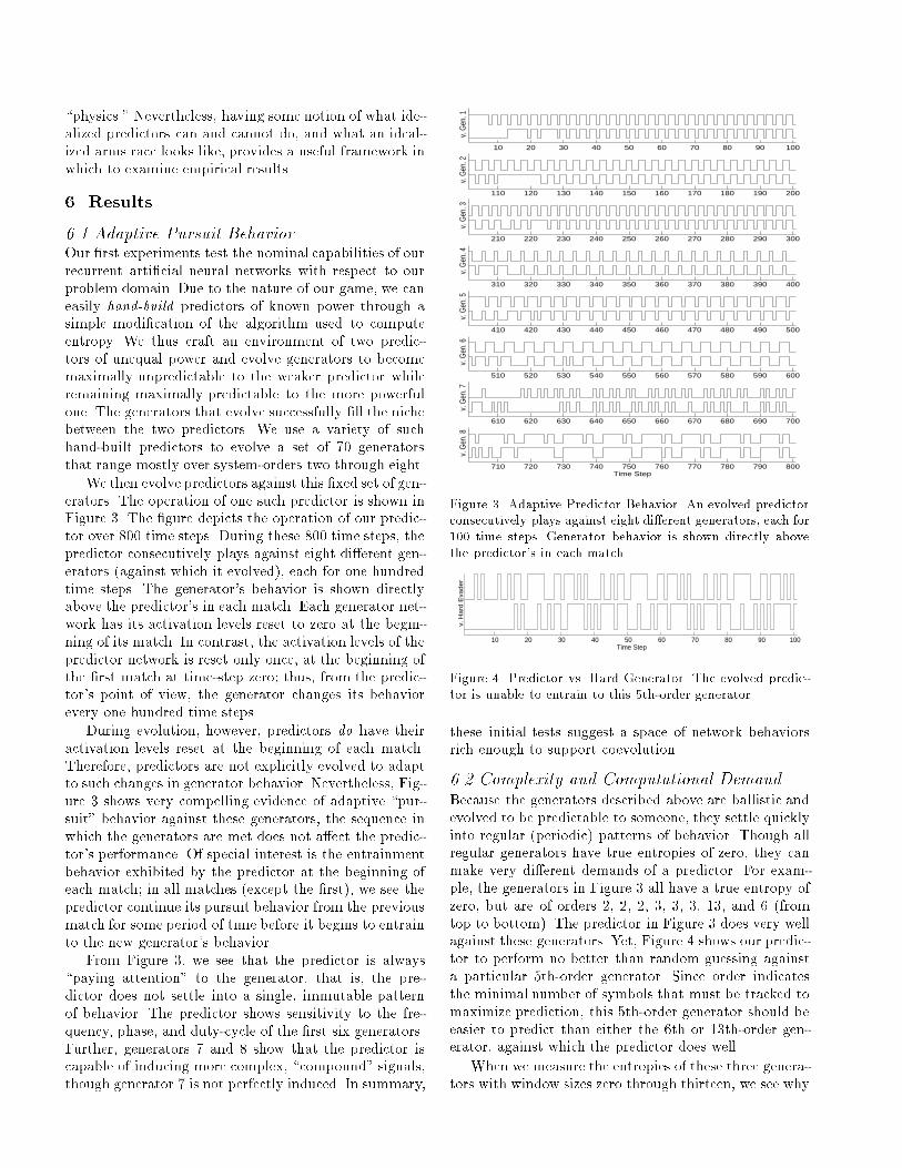
We then evolve predictors against this �xed set of gen-erators. The operation of one such predictor is shown inFigure 3. The �gure depicts the operation of our predic-tor over 800 time steps. During these 800 time steps, thepredictor consecutively plays against eight di�erent gen-erators (against which it evolved), each for one hundredtime steps. The generator's behavior is shown directlyabove the predictor's in each match. Each generator net-work has its activation levels reset to zero at the begin-ning of its match. In contrast, the activation levels of thepredictor network is reset only once, at the beginning ofthe �rst match at time-step zero; thus, from the predic-tor's point of view, the generator changes its behaviorevery one hundred time steps.

During evolution, however, predictors do have theiractivation levels reset at the beginning of each match.Therefore, predictors are not explicitly evolved to adaptto such changes in generator behavior. Nevertheless, Fig-ure 3 shows very compelling evidence of adaptive \pur-suit" behavior against these generators; the sequence inwhich the generators are met does not a�ect the predic-tor's performance. Of special interest is the entrainmentbehavior exhibited by the predictor at the beginning ofeach match; in all matches (except the �rst), we see thepredictor continue its pursuit behavior from the previousmatch for some period of time before it begins to entrainto the new generator's behavior.

From Figure 3, we see that the predictor is always\paying attention" to the generator, that is, the pre-dictor does not settle into a single, immutable patternof behavior. The predictor shows sensitivity to the fre-quency, phase, and duty-cycle of the �rst six generators.Further, generators 7 and 8 show that the predictor iscapable of inducing more complex, \compound" signals,though generator 7 is not perfectly induced. In summary,

10 20 30 40 50 60 70 80 90 100

v. G

en. 1

110 120 130 140 150 160 170 180 190 200

v. G

en. 2

210 220 230 240 250 260 270 280 290 300

v. G

en. 3

310 320 330 340 350 360 370 380 390 400

v. G

en. 4

410 420 430 440 450 460 470 480 490 500

v. G

en. 5

510 520 530 540 550 560 570 580 590 600

v. G

en. 6

610 620 630 640 650 660 670 680 690 700

v. G

en. 7

710 720 730 740 750 760 770 780 790 800v.

Gen

. 8Time Step

Figure 3 Adaptive Predictor Behavior. An evolved predictorconsecutively plays against eight di�erent generators, each for

100 time steps. Generator behavior is shown directly above

the predictor's in each match.

10 20 30 40 50 60 70 80 90 100

v. H

ard

Eva

de

r

Time Step

Figure 4 Predictor vs. Hard Generator. The evolved predic-

tor is unable to entrain to this 5th-order generator.

these initial tests suggest a space of network behaviorsrich enough to support coevolution.

6.2 Complexity and Computational DemandBecause the generators described above are ballistic andevolved to be predictable to someone, they settle quicklyinto regular (periodic) patterns of behavior. Though allregular generators have true entropies of zero, they canmake very di�erent demands of a predictor. For exam-ple, the generators in Figure 3 all have a true entropy ofzero, but are of orders 2, 2, 2, 3, 3, 3, 13, and 6 (fromtop to bottom). The predictor in Figure 3 does very wellagainst these generators. Yet, Figure 4 shows our predic-tor to perform no better than random guessing againsta particular 5th-order generator. Since order indicatesthe minimal number of symbols that must be tracked tomaximize prediction, this 5th-order generator should beeasier to predict than either the 6th or 13th-order gen-erator, against which the predictor does well.

When we measure the entropies of these three genera-tors with window sizes zero through thirteen, we see why

0 2 4 6 8 10 12 140

0.2

0.4

0.6

0.8

1

13th Order

5th Order6th Order

Window Size

Measu

red E

ntr

opy

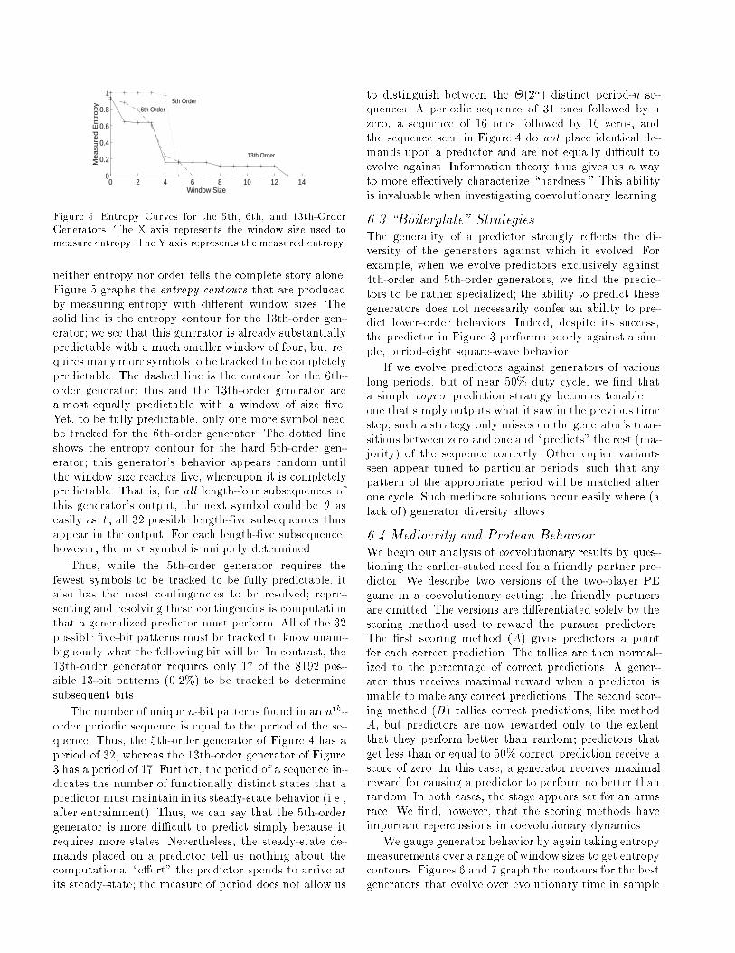
Figure 5 Entropy Curves for the 5th, 6th, and 13th-OrderGenerators. The X axis represents the window size used to

measure entropy. The Y axis represents the measured entropy.

neither entropy nor order tells the complete story alone.Figure 5 graphs the entropy contours that are producedby measuring entropy with di�erent window sizes. Thesolid line is the entropy contour for the 13th-order gen-erator; we see that this generator is already substantiallypredictable with a much smaller window of four, but re-quires manymore symbols to be tracked to be completelypredictable. The dashed line is the contour for the 6th-order generator; this and the 13th-order generator arealmost equally predictable with a window of size �ve.Yet, to be fully predictable, only one more symbol needbe tracked for the 6th-order generator. The dotted lineshows the entropy contour for the hard 5th-order gen-erator; this generator's behavior appears random untilthe window size reaches �ve, whereupon it is completelypredictable. That is, for all length-four subsequences ofthis generator's output, the next symbol could be 0 aseasily as 1 ; all 32 possible length-�ve subsequences thusappear in the output. For each length-�ve subsequence,however, the next symbol is uniquely determined.

Thus, while the 5th-order generator requires thefewest symbols to be tracked to be fully predictable, italso has the most contingencies to be resolved; repre-senting and resolving these contingencies is computationthat a generalized predictor must perform. All of the 32possible �ve-bit patterns must be tracked to know unam-biguously what the following bit will be. In contrast, the13th-order generator requires only 17 of the 8192 pos-sible 13-bit patterns (0.2%) to be tracked to determinesubsequent bits.

The number of unique n-bit patterns found in an nth-order periodic sequence is equal to the period of the se-quence. Thus, the 5th-order generator of Figure 4 has aperiod of 32, whereas the 13th-order generator of Figure3 has a period of 17. Further, the period of a sequence in-dicates the number of functionally distinct states that apredictor mustmaintain in its steady-state behavior (i.e.,after entrainment). Thus, we can say that the 5th-ordergenerator is more di�cult to predict simply because itrequires more states. Nevertheless, the steady-state de-mands placed on a predictor tell us nothing about thecomputational \e�ort" the predictor spends to arrive atits steady-state; the measure of period does not allow us

to distinguish between the �(2n) distinct period-n se-quences. A periodic sequence of 31 ones followed by azero, a sequence of 16 ones followed by 16 zeros, andthe sequence seen in Figure 4 do not place identical de-mands upon a predictor and are not equally di�cult toevolve against. Information theory thus gives us a wayto more e�ectively characterize \hardness." This abilityis invaluable when investigating coevolutionary learning.

6.3 \Boilerplate" StrategiesThe generality of a predictor strongly re ects the di-versity of the generators against which it evolved. Forexample, when we evolve predictors exclusively against4th-order and 5th-order generators, we �nd the predic-tors to be rather specialized; the ability to predict thesegenerators does not necessarily confer an ability to pre-dict lower-order behaviors. Indeed, despite its success,the predictor in Figure 3 performs poorly against a sim-ple, period-eight square-wave behavior.

If we evolve predictors against generators of variouslong periods, but of near 50% duty cycle, we �nd thata simple copier prediction strategy becomes tenable |one that simply outputs what it saw in the previous timestep; such a strategy only misses on the generator's tran-sitions between zero and one and \predicts" the rest (ma-jority) of the sequence correctly. Other copier variantsseen appear tuned to particular periods, such that anypattern of the appropriate period will be matched afterone cycle. Such mediocre solutions occur easily where (alack of) generator diversity allows.

6.4 Mediocrity and Protean BehaviorWe begin our analysis of coevolutionary results by ques-tioning the earlier-stated need for a friendly partner pre-dictor. We describe two versions of the two-player PEgame in a coevolutionary setting; the friendly partnersare omitted. The versions are di�erentiated solely by thescoring method used to reward the pursuer predictors.The �rst scoring method (A) gives predictors a pointfor each correct prediction. The tallies are then normal-ized to the percentage of correct predictions. A gener-ator thus receives maximal reward when a predictor isunable to make any correct predictions. The second scor-ing method (B) tallies correct predictions, like methodA, but predictors are now rewarded only to the extentthat they perform better than random; predictors thatget less than or equal to 50% correct prediction receive ascore of zero. In this case, a generator receives maximalreward for causing a predictor to perform no better thanrandom. In both cases, the stage appears set for an armsrace. We �nd, however, that the scoring methods haveimportant repercussions in coevolutionary dynamics.

We gauge generator behavior by again taking entropymeasurements over a range of window sizes to get entropycontours. Figures 6 and 7 graph the contours for the bestgenerators that evolve over evolutionary time in sample

runs for scoring methods A and B, respectively. Bothgraphs show that generator behavior remains consistentover the course of the run; we have no indication of anarms race. The generators coevolved with method A aresubstantially predictable and regular, as evidenced bythe rapidly dropping contours. The generators coevolvedwith methodB, on the other hand, are considerably moreirregular (unpredictable), as the contours decline gradu-ally and consume a much greater volume of space in thegraph. This contrast in outcome is found even in pairs ofruns that start with identical initial populations.

050

100150

200250

300350

0 2 4 6 8 10 12 14

00.20.40.60.8

1

Generation

Window Size

En

tro

py

Figure 6 Scoring Method A| Reward for Each Correct Pre-

diction. Rapidly declining entropy contours indicate substan-tially predictable behavior.

0

50

100

150

200

0 2 4 6 8 10 12 14

00.20.40.60.8

1

Generation

Window Size

En

tro

py

Figure 7 Scoring Method B | Reward for Predicting Better

than Random. Gradually declining entropy contours indicate

signi�cantly more complex behavior than that seen by scoring

method A.

The di�erence between scoring methods is manifestedquickly, if not immediately. Since the initial conditionsare similar (or, indeed, identical if we wish) we knowthat we have isolated a selection pressure that stems sim-ply from how games are scored: regular behavior is moreadaptive to scoring method A than is irregular behav-ior. That regular generators out-score irregular ones bymethod A indicates that simple prediction strategies canbe elicited from the predictor population | prediction

strategies against which the most adaptive generatorsact as potent anti-signals, sequences that make predic-tors perform worse than random (Zhu and Kinzel, 1997).Indeed, the champion generators shown in Figure 6 re-ceive scores that indicate exactly this. Nevertheless, if theballistic generators are to be viable as anti-signals, thenthere must exist some su�cient amount of homogeneitywithin the predictor population. This homogeneity ap-pears to reverberate through the system; rather than en-ter an arms race, the two populations fall into a circularpattern of mutual specialization, or convention chasing

| a mediocre stable-state.In contrast, scoring method B selects for an irregu-

lar behavior that reasonably captures the notion of pro-teanism in the PE game. Figure 8 provides a sampleof behavior from a typical generator produced by thisrun. This behavior is adaptive because it guarantees aminimal predictor score, regardless of what the predic-tor does, short of specialized memorization. Indeed, whilethe generators in Figure 7 are not actually fully irregu-lar, they are complex enough to cause the best predic-tors from this run to score only an average of 6% betterthan random guessing (53% correct prediction); that is,these generators are near optimal with respect to theirpredictor opponents. By de�ning an optimal strategy,namely random behavior, method B makes the gameclosed-ended.

20 40 60 80 100 120 140 160 180 200

Pro

tea

n E

vad

er

Time Step

Figure 8 Typical Behavior of a Protean Generator.

6.5 Pursuing a Communicative ConventionThe above results suggest that the two-player PE for-mulation may be problematic if we wish to develop anopen-ended arms race. Particularly, the two-player gamemay oversimplify the ecology by inadequately placingconstraints upon generator behavior. In the three-playerPE game, we maintain scoring method B to promotecomplexity and simply add the friendly predictor part-ner. Now, the evader and friendly partner must establisha convention of behavior that allows the partner to en-train to (coordinate with) the evader, but not the hostilepursuer. We �nd that the tension created by the need to\mate" with (be predictable to) the partner profoundlya�ects evasion behavior. Far from extinguishing heatedcompetition, the triangle of relationships gives rise tomuch more lively system dynamics than those found inthe absence of friendly partners.

In contrast with Figures 6 and 7, Figure 9 shows thatgenerator complexity in the three-player game is not atall consistent over evolutionary time; we see an overall

020

4060

80100

0 2 4 6 8 10 12 14

00.20.40.60.8

1

Generation

Window Size

En

tro

py

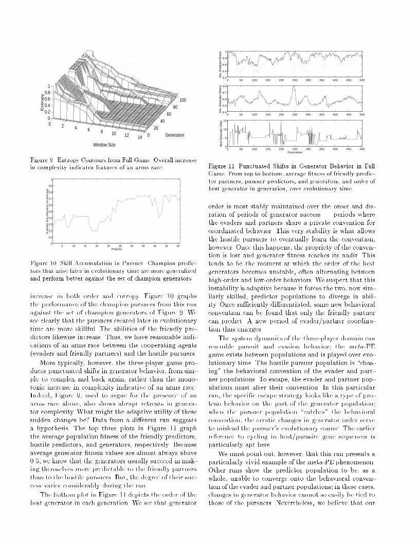
Figure 9 Entropy Contours from Full Game. Overall increasein complexity indicates features of an arms race.

5 10 15 20 25 30 35 40 45 50 550

0.1

0.2

0.3

0.4

0.5

0.6

0.7

0.8

0.9

1

Predictor

% B

ett

er

tha

n R

an

do

m o

n A

ve

rag

e

Figure 10 Skill Accumulation in Pursuer. Champion predic-

tors that arise later in evolutionary time are more generalized

and perform better against the set of champion generators.

increase in both order and entropy. Figure 10 graphsthe performance of the champion pursuers from this runagainst the set of champion generators of Figure 9. Wesee clearly that the pursuers created later in evolutionarytime are more skillful. The abilities of the friendly pre-dictors likewise increase. Thus, we have reasonable indi-cations of an arms race between the cooperating agents(evaders and friendly partners) and the hostile pursuers.

More typically, however, the three-player game pro-duces punctuated shifts in generator behavior, from sim-ple to complex and back again, rather than the mono-tonic increase in complexity indicative of an arms race.Indeed, Figure 9, used to argue for the presence of anarms race above, also shows abrupt retreats in genera-tor complexity. What might the adaptive utility of thesesudden changes be? Data from a di�erent run suggestsa hypothesis. The top three plots in Figure 11 graphthe average population �tness of the friendly predictors,hostile predictors, and generators, respectively. Becauseaverage generator �tness values are almost always above0.5, we know that the generators usually succeed in mak-ing themselves more predictable to the friendly partnersthan to the hostile pursuers. But, the degree of their suc-cess varies considerably during the run.

The bottom plot in Figure 11 depicts the order of thebest generator in each generation. We see that generator

0 50 100 150 200 250 300 350 400 450 5000.2

0.4

0.6

0.8

1

Ave

. Pre

dict

or F

itnes

s

0 50 100 150 200 250 300 350 400 450 5000.4

0.5

0.6

0.7

0.8

Ave

. Gen

erat

or F

itnes

s

0 50 100 150 200 250 300 350 400 450 5000

5

10

15

Generation

Bes

t Gen

erat

or O

rder

Figure 11 Punctuated Shifts in Generator Behavior in Full

Game. From top to bottom, average �tness of friendly predic-

tor partners, pursuer predictors, and generators, and order ofbest generator in generation, over evolutionary time.

order is most stably maintained over the onset and du-ration of periods of generator success | periods wherethe evaders and partners share a private convention forcoordinated behavior. This very stability is what allowsthe hostile pursuers to eventually learn the convention,however. Once this happens, the propriety of the conven-tion is lost and generator �tness reaches its nadir. Thistends to be the moment at which the order of the bestgenerators becomes unstable, often alternating betweenhigh-order and low-order behaviors. We suspect that thisinstability is adaptive because it forces the two, now sim-ilarly skilled, predictor populations to diverge in abil-ity. Once su�ciently di�erentiated, some new behavioralconvention can be found that only the friendly partnercan predict. A new period of evader/partner coordina-tion thus emerges.

The system dynamics of the three-player domain canresemble pursuit and evasion behavior; the meta-PEgame exists between populations and is played over evo-lutionary time. The hostile pursuer population is \chas-ing" the behavioral convention of the evader and part-ner populations. To escape, the evader and partner pop-ulations must alter their convention. In this particularrun, the speci�c escape strategy looks like a type of pro-tean behavior on the part of the generator population;when the pursuer population \catches" the behavioralconvention, the erratic changes in generator order serveto mislead the pursuer's evolutionary course. The earlierreference to cycling in host/parasite gene sequences isparticularly apt here.

We must point out, however, that this run presents aparticularly vivid example of the meta-PE phenomenon.Other runs show the predictor population to be, as awhole, unable to converge onto the behavioral conven-tion of the evader and partner populations; in these cases,changes in generator behavior cannot so easily be tied tothose of the pursuers. Nevertheless, we believe that our

methodology will allow us to clarify our data by contin-uing work with hand-built environments.

7. Conclusions

We show that pursuer-evader can be reformulated as aone-dimensional, time-series prediction game. Informa-tion theoretic tools provide quantitative analyses andhelp operationalize the domain. Because the linear PEgame emphasizes the informational (in the technicalsense) aspects of pursuit and evasion behavior, it cap-tures a fundamental aspect of communication.

Our behavioral metrics also yield informative viewsof coevolutionary dynamics. Though we can create goodevaders and pursuers with simple evolution, we �ndthat successful coevolution does not automatically fol-low. Subtleties in scoring method strongly in uence theoutcome of the two-player game; one method leads tomediocrity while the other de�nes an optimal strategy(protean behavior) and closes the world. The combina-tion of competitive and convergent pressures of the three-player game is needed to avoid simple mediocre stable-states while keeping an open world.

Tools exist to characterize generator behavior andhand-build predictors of known power. This toolset hasrecently been augmented to include new methods thatallow us to construct by hand generators with particularentropy contours and systematically analyze the general-ity and power of evolved predictors. Our future work willfeature these techniques in a continued investigation ofgenerator complexity, the computational demands gen-erators place on predictors, and the ease with which pre-dictors evolve against them. The �nal results we reportare not fully understood and will require these tools toelucidate.

8. Acknowledgments

The authors gratefully acknowledge the many hours ofconversation that have contributed to this work providedby Alan Blair, Marty Cohn, Paul Darwen, Pablo Funes,Greg Hornby, Ofer Melnik, Jason Noble, Elizabeth Sklar,and particularly Richard Watson.

References

Ackley, D. H. and Littman, M. L. (1994). Altruism in the

evolution of communication. In (Brooks and Maes, 1994),

pages 40{48.Akiyama, E. and Kaneko, K. (1997). Evolution of commu-

nication and strategies in an iterated three-person game.

In Langton, C. G. and Shimohara, K., editors, Arti�cialLife V (1996), pages 150{158. MIT Press.

Angeline, P. J. and Pollack, J. B. (1994). Competitive en-

vironments evolve better solutions for complex tasks. InForrest, S., editor, Proceedings of the Fifth International

Conference on Genetic Algorithms. Morgan Kaufmann.

Angeline, P. J., Saunders, G. M., and Pollack, J. B. (1994).An evolutionary algorithm that constructs recurrent neu-

ral networks. IEEE Transactions on Neural Networks,

5:54{65.Brooks, R. A. and Maes, P., editors (1994). Arti�cial Life

IV. MIT Press.

Cli�, D. and Miller, G. F. (1995). Tracking the red queen:Measurments of adaptive progress in co-evolutionary sim-

ulations. In Moran, F. et al., editors, Third European

Conference on Arti�cial Life, pages 200{218. SpringerVerlag.

Cli�, D. and Miller, G. F. (1996). Co-evolution of pursuit

and evasion 2: Simulation methods and results. In (Maeset al., 1996), pages 506{515.

Crutch�eld, J. P. (1994). The calculi of emergence: Compu-

tation, dynamics, and induction. Physica D, 75:11{54.Di Paolo, E. A. (1997). Social coordination and spatial orga-

nization: Steps towards the evolution of communication.

In Husbands, P. and Harvey, I., editors, Fourth EuropeanConference on Arti�cial Life, pages 464{473. MIT Press.

Gregory M. Saunders, J. B. P. (1996). The evolution of com-

munication schemes over continuous channaels. In (Maeset al., 1996), pages 580{589.

Hamilton, W. D., Axelrod, R., and Tanese, R. (1990). Sex-

ual reproduction as an adaptation to resist parasites (areview). Proc. Natl. Acad. Sci. USA, 87:3566{3573.

Hamming, R. W. (1980). Coding and Information Theory.

Prentice-Hall, Inc., Englewood Cli�s, NJ.Hashimoto, T. and Ikegami, T. (1996). Emergence of net-

grammar in communicating agents. BioSystems, 38(1):1{

14.Isaacs, R. (1965). Di�erential Games. John Wiley and Sons,

New York.

Kaneko, K. and Suzuki, J. (1994). Evolution to the edge ofchaos in an imitation game. In Langton, C. G., editor,

Arti�cial Life III (1992), pages 43{54. Addison-Wesley.

Koza, J. (1992). Genetic Programming. MIT Press.Langton, C. G. and Shimohara, K., editors (1997). Arti�cial

Life V (1996). MIT Press.

Maes, P. et al., editors (1996). From Animals to Animats IV.MIT Press.

Miller, G. F. and Cli�, D. (1994). Protean behavior in dy-

namic games: Arguments for the co-evolution of pursuit-evasion tactics. In Cli�, D. et al., editors, From Animals

to Animats III, pages 411{420. MIT Press.

Oliphant, M. and Batali, J. (1996). Learning and the emer-gence of coordinated communication. (Submitted).

Pollack, J. B., Blair, A., and Land, M. (1997). Coevolution

of a backgammon player. In (Langton and Shimohara,1997).

Reynolds, C. (1994). Competition, coevolution and the game

of tag. In (Brooks and Maes, 1994), pages 59{69.

Steels, L. (1997). Self-organising vocabularies. In (Langton

and Shimohara, 1997), pages 136{141.

Werner, G. M. and Dyer, M. G. (1991). Evolution of commu-

nication in arti�cial organisms. In Langton, C., Taylor,

C., Farmer, J., and Rasmussen, S., editors, Arti�cial Life

II (1990), pages 659{687. Addison-Wesley.

Zhu, H. and Kinzel, W. (1997). Anti-predictable sequences:

Harder to predict than a random sequence. (Submitted).