CN Lab Manual_algo

Computer Networks Lab Manual

BIT,BANGALORE-04

Department Of Computer Science and Engineering Page 0

COMPUTER NETWORKS

LAB MANUAL

For

VII SEMESTER

Prepared by:

Jyothi. D.G & Girija. J, Dept. of CSE,

DEPARTMENT OF COMPUTER SCIENCE &

ENGINEERING

BANGALORE INSTITUTE OF TECHNOLOGY K R ROAD, V V PURAM

BANGALORE-560004


BIT,BANGALORE-04


NETWORKS LABORATORY (COMMON TO CSE & ISE)

Sub Code : CSL77 Note : Student is required to solve one problem from PART-A and one problem

from PART-B. Both the parts have equal weightage.

PART A – Simulation Exercises The following experiments shall be conducted using either NS228/OPNET or any other simulators. 1. Simulate a three nodes point-to-point network with duplex links between them. Set

the queue size vary the bandwidth and find the number of packets dropped. 2. Simulate a four node point-to-point network, and connect the links as follows: n0-n2,

n1-n2 and n2-n3. Apply TCP agent between n0-n3 and UDP n1-n3. Apply relevant applications over TCP and UDP agents changing the parameter and determine the number of packets by TCP/UDP.

3. Simulate the different types of Internet traffic such as FTP a TELNET over a network and analyze the throughput.

4. Simulate the transmission of ping messaged over a network topology consisting of 6 nodes and find the number of packets dropped due to congestion.

5. Simulate an Ethernet LAN using N-nodes(6-10), change error rate and data rate and compare the throughput.

6. Simulate an Ethernet LAN using N nodes and set multiple traffic nodes and determine collision across different nodes.

7. Simulate an Ethernet LAN using N nodes and set multiple traffic nodes and plot congestion window for different source/destination.

8. Simulate simple ESS and with transmitting nodes in wire-less LAN by simulation and determine the performance with respect to transmission of packets.

PART B

The following experiments shall be conducted using C/C++. 1. Write a program for error detecting code using CRC-CCITT (16-bits). 2. Write a program for frame sorting technique used in buffers. 3. Write a program for distance vector algorithm to find suitable path for transmission. 4. Using TCP/IP sockets, write a client-server program to make client sending the file

name and the server to send back the contents of the requested file if present. 5. Implement the above program using as message queues or FIFOs as IPC channels. 6. Write a program for simple RSA algorithm to encrypt and decrypt the data. 7. Write a program for Hamming Code generation for error detection and correction. 8. Write a program for congestion control using Leaky bucket algorithm.


BIT,BANGALORE-04


PART A Programs

Start up

1. Open three terminals a) in terminal 1 at command prompt run dispatcher( root@localhost#

dispatcher) b) in terminal 2 at command prompt run coordinator( root@localhost#

coordinator) c) in terminal 3 at command prompt run nctunsclient( root@localhost#

nctunsclient)

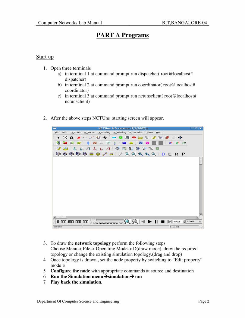
2. After the above steps NCTUns starting screen will appear.

3. To draw the network topology perform the following steps Choose Menu-> File-> Operating Mode-> D(draw mode), draw the required topology or change the existing simulation topology.(drag and drop)

4 Once topology is drawn , set the node property by switching to “Edit property” mode E

5 Configure the node with appropriate commands at source and destination 6 Run the Simulation menu��simulation��run 7 Play back the simulation.


BIT,BANGALORE-04


Experiment No 1

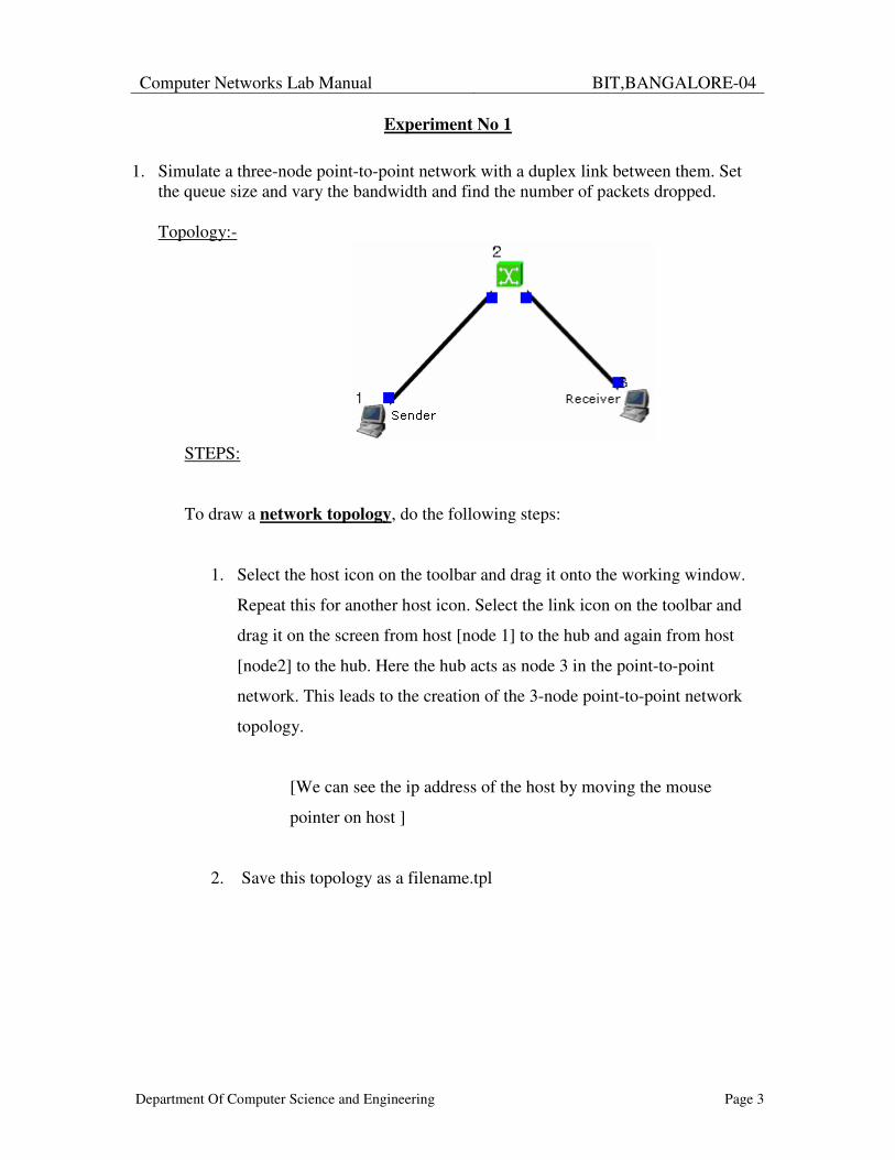
1. Simulate a three-node point-to-point network with a duplex link between them. Set the queue size and vary the bandwidth and find the number of packets dropped. Topology:-

STEPS:

To draw a network topology, do the following steps:

1. Select the host icon on the toolbar and drag it onto the working window.

Repeat this for another host icon. Select the link icon on the toolbar and

drag it on the screen from host [node 1] to the hub and again from host

[node2] to the hub. Here the hub acts as node 3 in the point-to-point

network. This leads to the creation of the 3-node point-to-point network

topology.

[We can see the ip address of the host by moving the mouse

pointer on host ]

2. Save this topology as a filename.tpl


BIT,BANGALORE-04


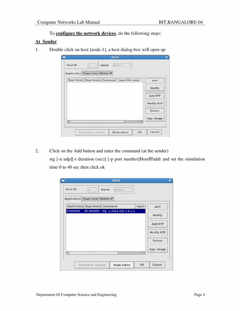
To configure the network devices, do the following steps:

At Sender

1. Double click on host [node-1], a host dialog box will open up

2. Click on the Add button and enter the command (at the sender)

stg [-u udp][-t duration (sec)] [-p port number]HostIPaddr and set the simulation

time 0 to 40 sec then click ok


BIT,BANGALORE-04


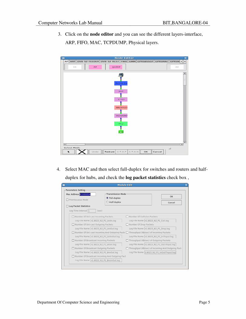
3. Click on the node editor and you can see the different layers-interface,

ARP, FIFO, MAC, TCPDUMP, Physical layers.

4. Select MAC and then select full-duplex for switches and routers and half-

duplex for hubs, and check the log packet statistics check box ,


BIT,BANGALORE-04


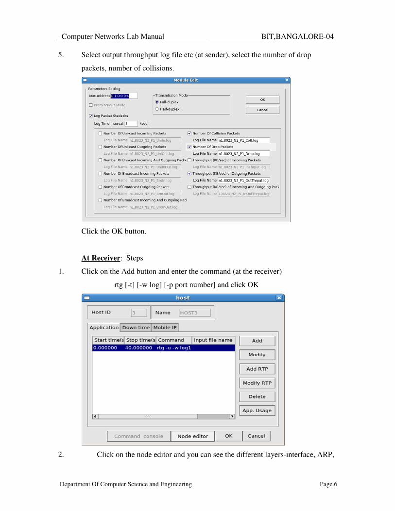
5. Select output throughput log file etc (at sender), select the number of drop

packets, number of collisions.

Click the OK button.

At Receiver: Steps

1. Click on the Add button and enter the command (at the receiver)

rtg [-t] [-w log] [-p port number] and click OK

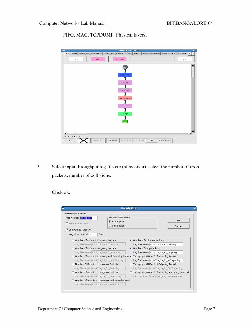
2. Click on the node editor and you can see the different layers-interface, ARP,


BIT,BANGALORE-04


FIFO, MAC, TCPDUMP, Physical layers.

3. Select input throughput log file etc (at receiver), select the number of drop


Click ok.


BIT,BANGALORE-04


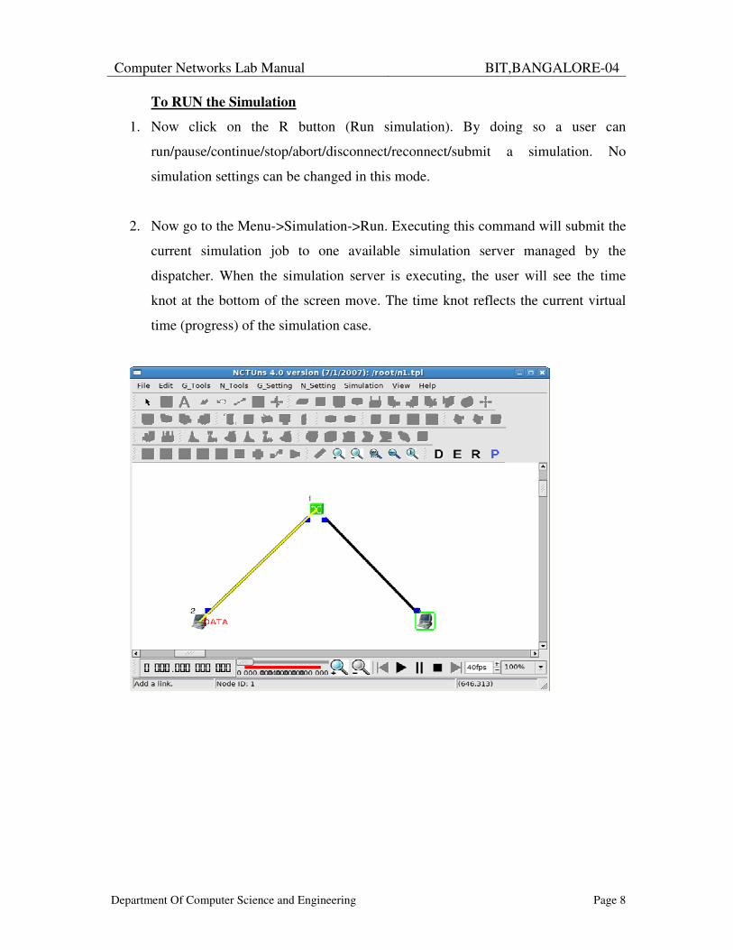
To RUN the Simulation

1. Now click on the R button (Run simulation). By doing so a user can

run/pause/continue/stop/abort/disconnect/reconnect/submit a simulation. No

simulation settings can be changed in this mode.

2. Now go to the Menu->Simulation->Run. Executing this command will submit the

current simulation job to one available simulation server managed by the

dispatcher. When the simulation server is executing, the user will see the time

knot at the bottom of the screen move. The time knot reflects the current virtual

time (progress) of the simulation case.


BIT,BANGALORE-04


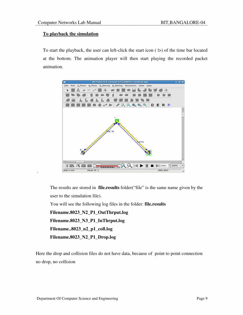
To playback the simulation

To start the playback, the user can left-click the start icon ( |>) of the time bar located

at the bottom. The animation player will then start playing the recorded packet

animation.

.

The results are stored in file.results folder(“file” is the same name given by the

user to the simulation file).

You will see the following log files in the folder: file.results

Filename.8023_N2_P1_OutThrput.log

Filename.8023_N3_P1_InThrput.log

Filename..8023_n2_p1_coll.log

Filename.8023_N2_P1_Drop.log

Here the drop and collision files do not have data, because of point to point connection

no drop, no collision


BIT,BANGALORE-04


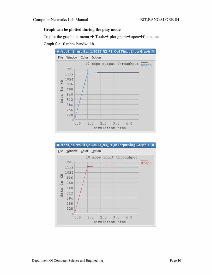
Graph can be plotted during the play mode

To plot the graph on menu � Tools� plot graph�open�file name

Graph for 10 mbps bandwidth


BIT,BANGALORE-04


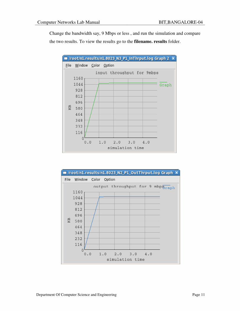
Change the bandwidth say, 9 Mbps or less , and run the simulation and compare

the two results. To view the results go to the filename. results folder.


BIT,BANGALORE-04


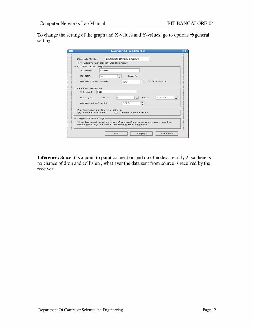
To change the setting of the graph and X-values and Y-values ,go to options �general setting

Inference: Since it is a point to point connection and no of nodes are only 2 ,so there is no chance of drop and collision , what ever the data sent from source is received by the receiver.


BIT,BANGALORE-04


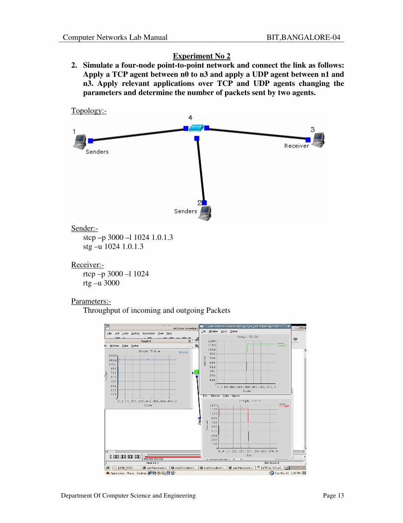
Experiment No 2 2. Simulate a four-node point-to-point network and connect the link as follows:

Apply a TCP agent between n0 to n3 and apply a UDP agent between n1 and n3. Apply relevant applications over TCP and UDP agents changing the parameters and determine the number of packets sent by two agents.

Topology:-

Sender:- stcp –p 3000 –l 1024 1.0.1.3 stg –u 1024 1.0.1.3 Receiver:- rtcp –p 3000 –l 1024 rtg –u 3000 Parameters:- Throughput of incoming and outgoing Packets


BIT,BANGALORE-04


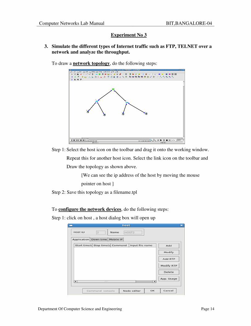
Experiment No 3

3. Simulate the different types of Internet traffic such as FTP, TELNET over a network and analyze the throughput.

To draw a network topology, do the following steps:

Step 1: Select the host icon on the toolbar and drag it onto the working window.

Repeat this for another host icon. Select the link icon on the toolbar and

Draw the topology as shown above.

[We can see the ip address of the host by moving the mouse

pointer on host ]

Step 2: Save this topology as a filename.tpl

To configure the network devices, do the following steps:

Step 1: click on host , a host dialog box will open up


BIT,BANGALORE-04


Step 2: Click on the Add button and enter the command (at the sender)

node 1: For FTP stcp –p 21 –l 1024 1.0.1.4

node 2: For Telnet stcp –p 23 –l1024 1.0.1.4 and set the simulation time 0 to 40 sec then click ok

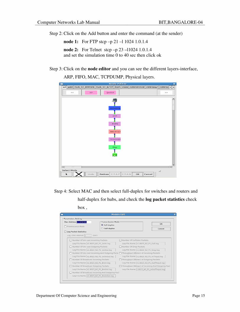
Step 3: Click on the node editor and you can see the different layers-interface,

ARP, FIFO, MAC, TCPDUMP, Physical layers.

Step 4: Select MAC and then select full-duplex for switches and routers and

half-duplex for hubs, and check the log packet statistics check

box ,


BIT,BANGALORE-04


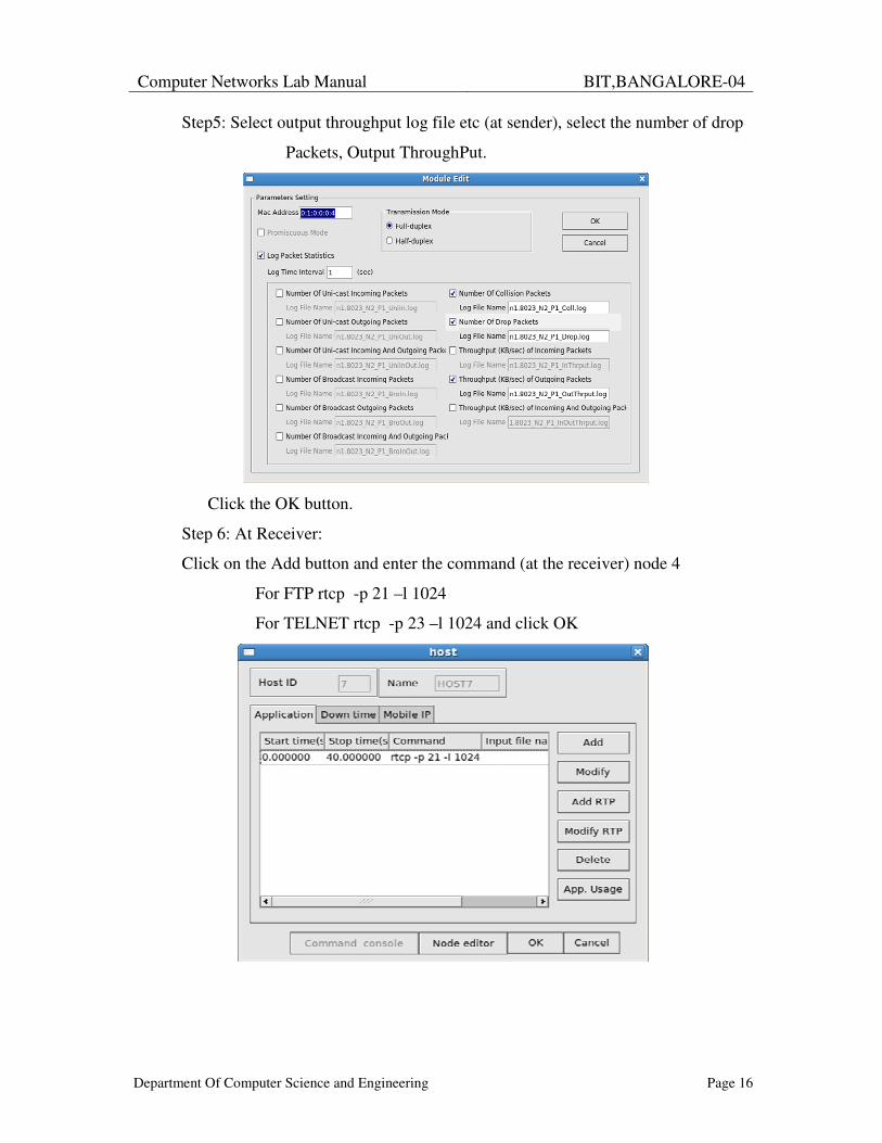
Step5: Select output throughput log file etc (at sender), select the number of drop

Packets, Output ThroughPut.

Click the OK button.

Step 6: At Receiver:

Click on the Add button and enter the command (at the receiver) node 4

For FTP rtcp -p 21 –l 1024

For TELNET rtcp -p 23 –l 1024 and click OK


BIT,BANGALORE-04


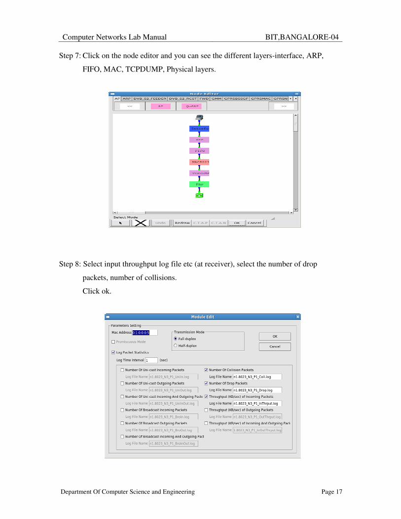
Step 7: Click on the node editor and you can see the different layers-interface, ARP,

FIFO, MAC, TCPDUMP, Physical layers.

Step 8: Select input throughput log file etc (at receiver), select the number of drop


Click ok.


BIT,BANGALORE-04


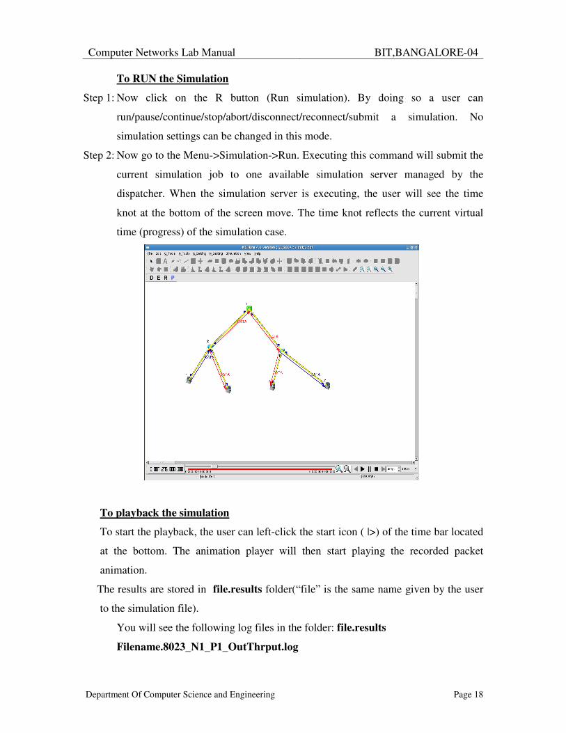
To RUN the Simulation

Step 1: Now click on the R button (Run simulation). By doing so a user can

run/pause/continue/stop/abort/disconnect/reconnect/submit a simulation. No

simulation settings can be changed in this mode.

Step 2: Now go to the Menu->Simulation->Run. Executing this command will submit the

current simulation job to one available simulation server managed by the

dispatcher. When the simulation server is executing, the user will see the time

knot at the bottom of the screen move. The time knot reflects the current virtual

time (progress) of the simulation case.

To playback the simulation

To start the playback, the user can left-click the start icon ( |>) of the time bar located

at the bottom. The animation player will then start playing the recorded packet

animation.

The results are stored in file.results folder(“file” is the same name given by the user

to the simulation file).

You will see the following log files in the folder: file.results

Filename.8023_N1_P1_OutThrput.log


BIT,BANGALORE-04


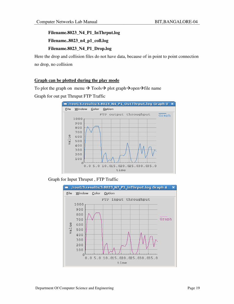
Filename.8023_N4_P1_InThrput.log

Filename..8023_n4_p1_coll.log

Filename.8023_N4_P1_Drop.log

Here the drop and collision files do not have data, because of in point to point connection

no drop, no collision

Graph can be plotted during the play mode

To plot the graph on menu � Tools� plot graph�open�file name

Graph for out put Thruput FTP Traffic

Graph for Input Thruput , FTP Traffic


BIT,BANGALORE-04


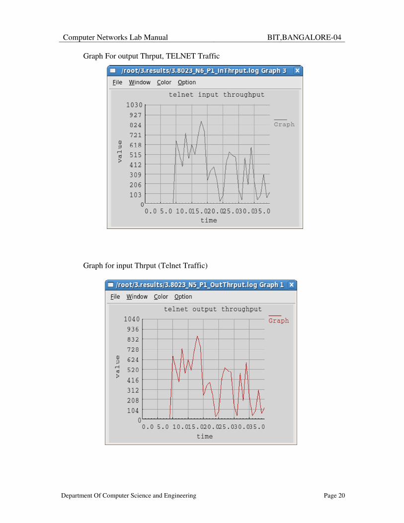
Graph For output Thrput, TELNET Traffic

Graph for input Thrput (Telnet Traffic)


BIT,BANGALORE-04


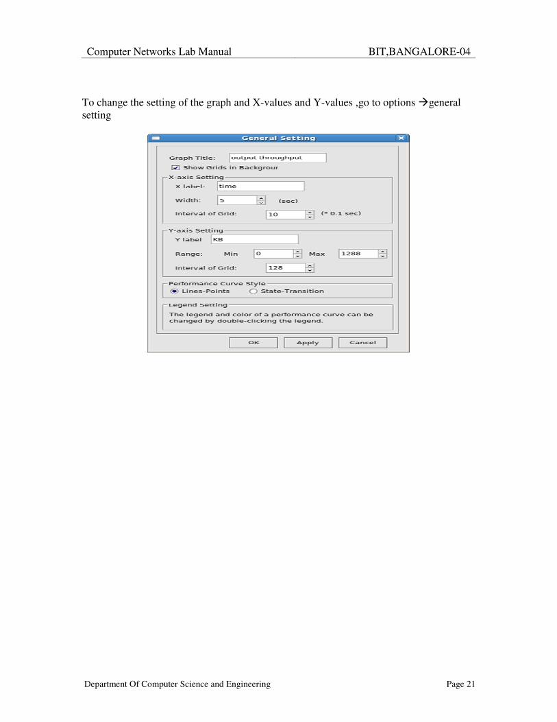
To change the setting of the graph and X-values and Y-values ,go to options �general setting


BIT,BANGALORE-04


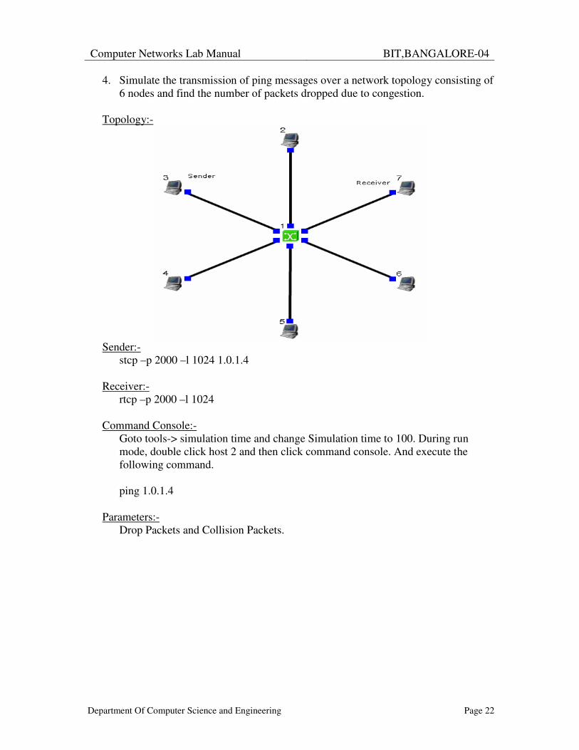
4. Simulate the transmission of ping messages over a network topology consisting of 6 nodes and find the number of packets dropped due to congestion.

Topology:-

Sender:- stcp –p 2000 –l 1024 1.0.1.4 Receiver:- rtcp –p 2000 –l 1024 Command Console:-

Goto tools-> simulation time and change Simulation time to 100. During run mode, double click host 2 and then click command console. And execute the following command. ping 1.0.1.4

Parameters:- Drop Packets and Collision Packets.


BIT,BANGALORE-04


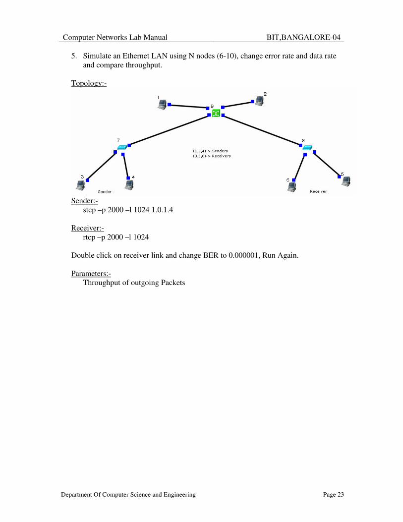
5. Simulate an Ethernet LAN using N nodes (6-10), change error rate and data rate and compare throughput.

Topology:-

Sender:- stcp –p 2000 –l 1024 1.0.1.4 Receiver:- rtcp –p 2000 –l 1024 Double click on receiver link and change BER to 0.000001, Run Again. Parameters:- Throughput of outgoing Packets


BIT,BANGALORE-04


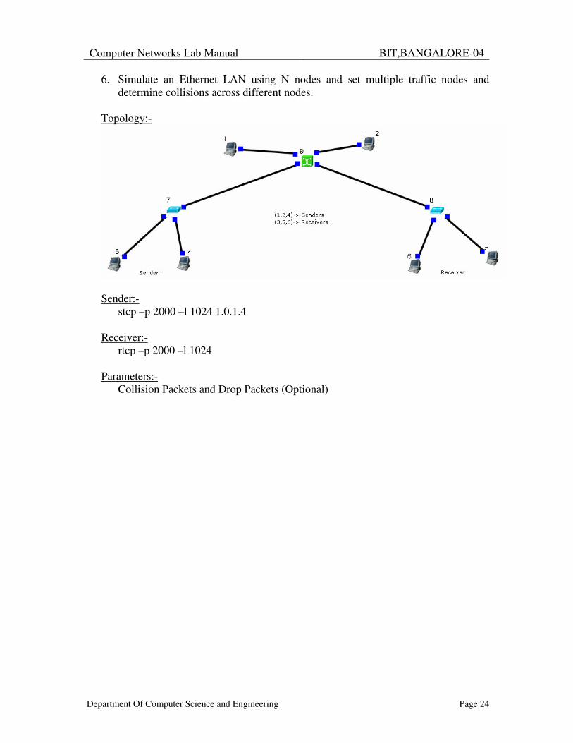
6. Simulate an Ethernet LAN using N nodes and set multiple traffic nodes and determine collisions across different nodes.

Topology:-

Sender:- stcp –p 2000 –l 1024 1.0.1.4 Receiver:- rtcp –p 2000 –l 1024 Parameters:-

Collision Packets and Drop Packets (Optional)


BIT,BANGALORE-04


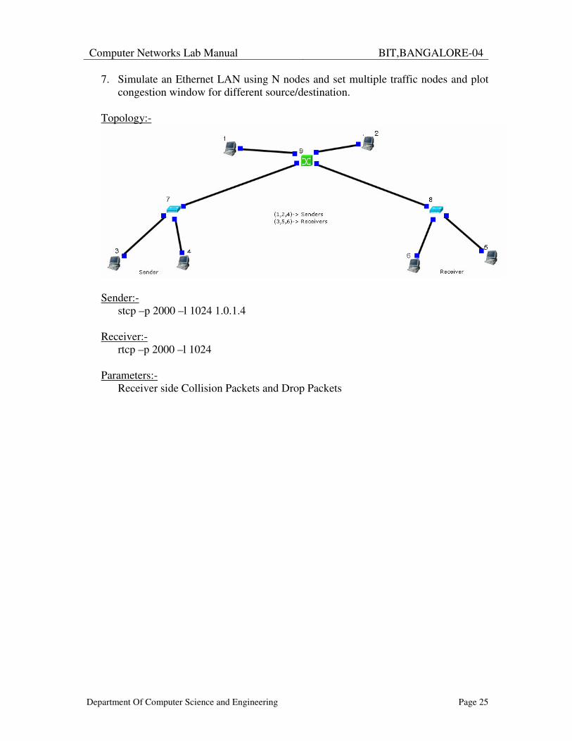
7. Simulate an Ethernet LAN using N nodes and set multiple traffic nodes and plot congestion window for different source/destination.

Topology:-

Sender:- stcp –p 2000 –l 1024 1.0.1.4 Receiver:- rtcp –p 2000 –l 1024 Parameters:-

Receiver side Collision Packets and Drop Packets


BIT,BANGALORE-04


8. Simulate simple BSS and with transmitting nodes in wireless LAN by simulation and determine the performance with respect to transmission of packets.

Topology:-

Click on “access point”. Goto wireless interface and tick on “show transmission range and then click OK. Double click on Router -> Node Editor and then Left stack -> throughput of Incoming packets Right stack -> throughput of Outgoing packets Select mobile hosts and access points then click on. Tools -> WLAN mobile nodes-> WLAN Generate infrastructure.

Subnet ID: Port number of router (2) Gateway ID: IP address of router

Mobile Host 1

ttcp –t –u –s –p 3000 1.0.1.1 Mobile Host 1

ttcp –t –u –s –p 3001 1.0.1.1 Host(Receiver)

ttcp –r –u –s –p 3000 ttcp –r –u –s –p 3001

Run and then play to plot the graph.


BIT,BANGALORE-04


Part B Programs

Experiment No 1 CRC

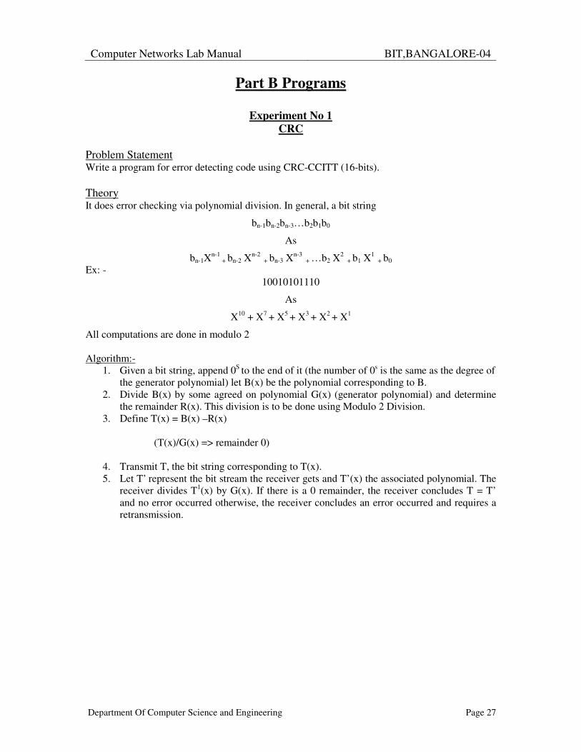
Problem Statement Write a program for error detecting code using CRC-CCITT (16-bits). Theory It does error checking via polynomial division. In general, a bit string

bn-1bn-2bn-3…b2b1b0

As

bn-1Xn-1 + bn-2 Xn-2

+ bn-3 Xn-3 + …b2 X2

+ b1 X1 + b0

Ex: - 10010101110

As

X10 + X7 + X5 + X3 + X2 + X1

All computations are done in modulo 2 Algorithm:-

1. Given a bit string, append 0S to the end of it (the number of 0s is the same as the degree of the generator polynomial) let B(x) be the polynomial corresponding to B.

2. Divide B(x) by some agreed on polynomial G(x) (generator polynomial) and determine the remainder R(x). This division is to be done using Modulo 2 Division.

3. Define T(x) = B(x) –R(x) (T(x)/G(x) => remainder 0)

4. Transmit T, the bit string corresponding to T(x). 5. Let T’ represent the bit stream the receiver gets and T’(x) the associated polynomial. The

receiver divides T1(x) by G(x). If there is a 0 remainder, the receiver concludes T = T’ and no error occurred otherwise, the receiver concludes an error occurred and requires a retransmission.


BIT,BANGALORE-04


Experiment No 2 Frame Sorting

Problem Statement Write a program for frame sorting technique used in buffers. Theory

The data link layer divides the stream of bits received from the network layer into manageable data units called frames.

If frames are to be distributed to different systems on the network, the Data link layer adds a header to the frame to define the sender and/or receiver of the frame.

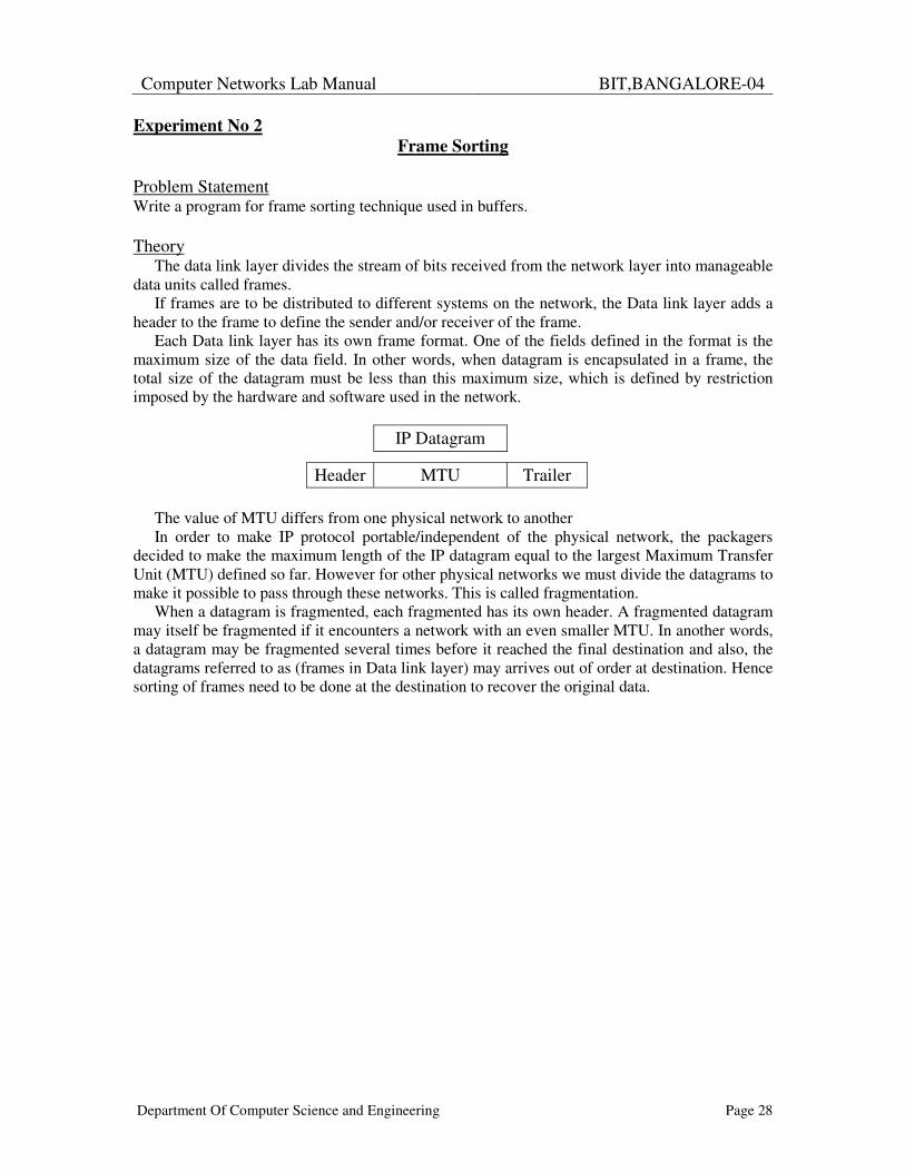
Each Data link layer has its own frame format. One of the fields defined in the format is the maximum size of the data field. In other words, when datagram is encapsulated in a frame, the total size of the datagram must be less than this maximum size, which is defined by restriction imposed by the hardware and software used in the network.

IP Datagram

Header MTU Trailer

The value of MTU differs from one physical network to another In order to make IP protocol portable/independent of the physical network, the packagers

decided to make the maximum length of the IP datagram equal to the largest Maximum Transfer Unit (MTU) defined so far. However for other physical networks we must divide the datagrams to make it possible to pass through these networks. This is called fragmentation.

When a datagram is fragmented, each fragmented has its own header. A fragmented datagram may itself be fragmented if it encounters a network with an even smaller MTU. In another words, a datagram may be fragmented several times before it reached the final destination and also, the datagrams referred to as (frames in Data link layer) may arrives out of order at destination. Hence sorting of frames need to be done at the destination to recover the original data.


BIT,BANGALORE-04


Experiment No 3 Distance Vector Routing

Problem Statement Write a program for distance vector algorithm to find suitable path for transmission. Theory

Routing algorithm is a part of network layer software which is responsible for deciding which output line an incoming packet should be transmitted on. If the subnet uses datagram internally, this decision must be made anew for every arriving data packet since the best route may have changed since last time. If the subnet uses virtual circuits internally, routing decisions are made only when a new established route is being set up. The latter case is sometimes called session routing, because a rout remains in force for an entire user session (e.g., login session at a terminal or a file).

Routing algorithms can be grouped into two major classes: adaptive and nonadaptive. Nonadaptive algorithms do not base their routing decisions on measurement or estimates of current traffic and topology. Instead, the choice of route to use to get from I to J (for all I and J) is compute in advance, offline, and downloaded to the routers when the network ids booted. This procedure is sometime called static routing.

Adaptive algorithms, in contrast, change their routing decisions to reflect changes in the topology, and usually the traffic as well. Adaptive algorithms differ in where they get information (e.g., locally, from adjacent routers, or from all routers), when they change the routes (e.g., every �T sec, when the load changes, or when the topology changes), and what metric is used for optimization (e.g., distance, number of hops, or estimated transit time).

Two algorithms in particular, distance vector routing and link state routing are the most popular. Distance vector routing algorithms operate by having each router maintain a table (i.e., vector) giving the best known distance to each destination and which line to get there. These tables are updated by exchanging information with the neighbors.

The distance vector routing algorithm is sometimes called by other names, including the distributed Bellman-Ford routing algorithm and the Ford-Fulkerson algorithm, after the researchers who developed it (Bellman, 1957; and Ford and Fulkerson, 1962). It was the original ARPANET routing algorithm and was also used in the Internet under the RIP and in early versions of DECnet and Novell’s IPX. AppleTalk and Cisco routers use improved distance vector protocols.

In distance vector routing, each router maintains a routing table indexed by, and containing one entry for, each router in subnet. This entry contains two parts: the preferred out going line to use for that destination, and an estimate of the time or distance to that destination. The metric used might be number of hops, time delay in milliseconds, total number of packets queued along the path, or something similar.

The router is assumed to know the “distance” to each of its neighbor. If the metric is hops, the distance is just one hop. If the metric is queue length, the router simply examines each queue. If the metric is delay, the router can measure it directly with special ECHO packets hat the receiver just time stamps and sends back as fast as possible.


BIT,BANGALORE-04


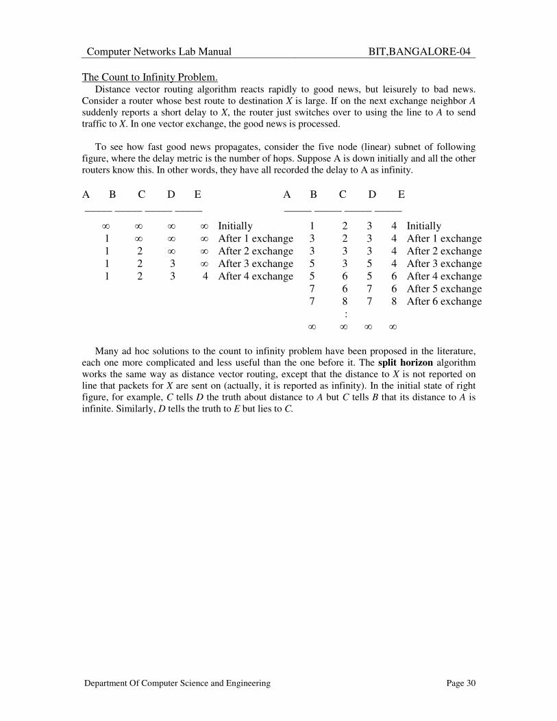
The Count to Infinity Problem. Distance vector routing algorithm reacts rapidly to good news, but leisurely to bad news.

Consider a router whose best route to destination X is large. If on the next exchange neighbor A suddenly reports a short delay to X, the router just switches over to using the line to A to send traffic to X. In one vector exchange, the good news is processed.

To see how fast good news propagates, consider the five node (linear) subnet of following figure, where the delay metric is the number of hops. Suppose A is down initially and all the other routers know this. In other words, they have all recorded the delay to A as infinity. A B C D E A B C D E _____ _____ _____ _____ _____ _____ _____ _____

� � � � Initially 1 2 3 4 Initially 1 � � � After 1 exchange 3 2 3 4 After 1 exchange 1 2 � � After 2 exchange 3 3 3 4 After 2 exchange 1 2 3 � After 3 exchange 5 3 5 4 After 3 exchange 1 2 3 4 After 4 exchange 5 6 5 6 After 4 exchange

7 6 7 6 After 5 exchange 7 8 7 8 After 6 exchange

:

� � � �

Many ad hoc solutions to the count to infinity problem have been proposed in the literature, each one more complicated and less useful than the one before it. The split horizon algorithm works the same way as distance vector routing, except that the distance to X is not reported on line that packets for X are sent on (actually, it is reported as infinity). In the initial state of right figure, for example, C tells D the truth about distance to A but C tells B that its distance to A is infinite. Similarly, D tells the truth to E but lies to C.


BIT,BANGALORE-04


Experiment No 4 TCP Socket

Problem Statement Using TCP/IP sockets, write a client-server program to make client sending the file name and the server to send back the contents of the requested file if present. Algorithm (Client Side)

1. Start. 2. Create a socket using socket() system call. 3. Connect the socket to the address of the server using connect() system call. 4. Send the filename of required file using send() system call. 5. Read the contents of the file sent by server by recv() system call. 6. Stop.

Algorithm (Server Side)

1. Start. 2. Create a socket using socket() system call. 3. Bind the socket to an address using bind() system call. 4. Listen to the connection using listen() system call. 5. accept connection using accept() 6. Receive filename and transfer contents of file with client. 7. Stop.


BIT,BANGALORE-04


Experiment No 5 FIFO IPC

Problem Statement Implement the above program using as message queues or FIFO as IPC channels. Algorithm (Client Side)

1. Start. 2. Open well known server FIFO in write mode. 3. Write the pathname of the file in this FIFO and send the request. 4. Open the client specified FIFO in read mode and wait for reply. 5. When the contents of the file are available in FIFO, display it on the terminal 6. Stop.

Algorithm (Server Side)

1. Start. 2. Create a well known FIFO using mkfifo() 3. Open FIFO in read only mode to accept request from clients. 4. When client opens the other end of FIFO in write only mode, then read the contents and

store it in buffer. 5. Create another FIFO in write mode to send replies. 6. Open the requested file by the client and write the contents into the client specified FIFO

and terminate the connection. 7. Stop.


BIT,BANGALORE-04


Experiment No 6 RSA Algorithm

Problem Statement Write a program for simple RSA algorithm to encrypt and decrypt the data. Theory

Cryptography has a long and colorful history. The message to be encrypted, known as the plaintext, are transformed by a function that is parameterized by a key. The output of the encryption process, known as the ciphertext, is then transmitted, often by messenger or radio. The enemy, or intruder, hears and accurately copies down the complete ciphertext. However, unlike the intended recipient, he does not know the decryption key and so cannot decrypt the ciphertext easily. The art of breaking ciphers is called cryptanalysis the art of devising ciphers (cryptography) and breaking them (cryptanalysis) is collectively known as cryptology.

There are several ways of classifying cryptographic algorithms. They are generally categorized based on the number of keys that are employed for encryption and decryption, and further defined by their application and use. The three types of algorithms are as follows: 1. Secret Key Cryptography (SKC): Uses a single key for both encryption and decryption. It is

also known as symmetric cryptography. 2. Public Key Cryptography (PKC): Uses one key for encryption and another for decryption. It

is also known as asymmetric cryptography. 3. Hash Functions: Uses a mathematical transformation to irreversibly "encrypt" information

Public-key cryptography has been said to be the most significant new development in cryptography. Modern PKC was first described publicly by Stanford University professor Martin Hellman and graduate student Whitfield Diffie in 1976. Their paper described a two-key crypto system in which two parties could engage in a secure communication over a non-secure communications channel without having to share a secret key.

Generic PKC employs two keys that are mathematically related although knowledge of one key does not allow someone to easily determine the other key. One key is used to encrypt the plaintext and the other key is used to decrypt the ciphertext. The important point here is that it does not matter which key is applied first, but that both keys are required for the process to work. Because pair of keys is required, this approach is also called asymmetric cryptography.

In PKC, one of the keys is designated the public key and may be advertised as widely as the owner wants. The other key is designated the private key and is never revealed to another party. It is straight forward to send messages under this scheme.

The RSA algorithm is named after Ron Rivest, Adi Shamir and Len Adleman, who invented it in 1977.�The RSA algorithm can be used for both public key encryption and digital signatures. Its security is based on the difficulty of factoring large integers. Algorithm 1. Generate two large random primes, P and Q, of approximately equal size. 2. Compute N = P x Q 3. Compute Z = (P-1) x (Q-1). 4. Choose an integer E, 1 < E < Z, such that GCD (E, Z) = 1


BIT,BANGALORE-04


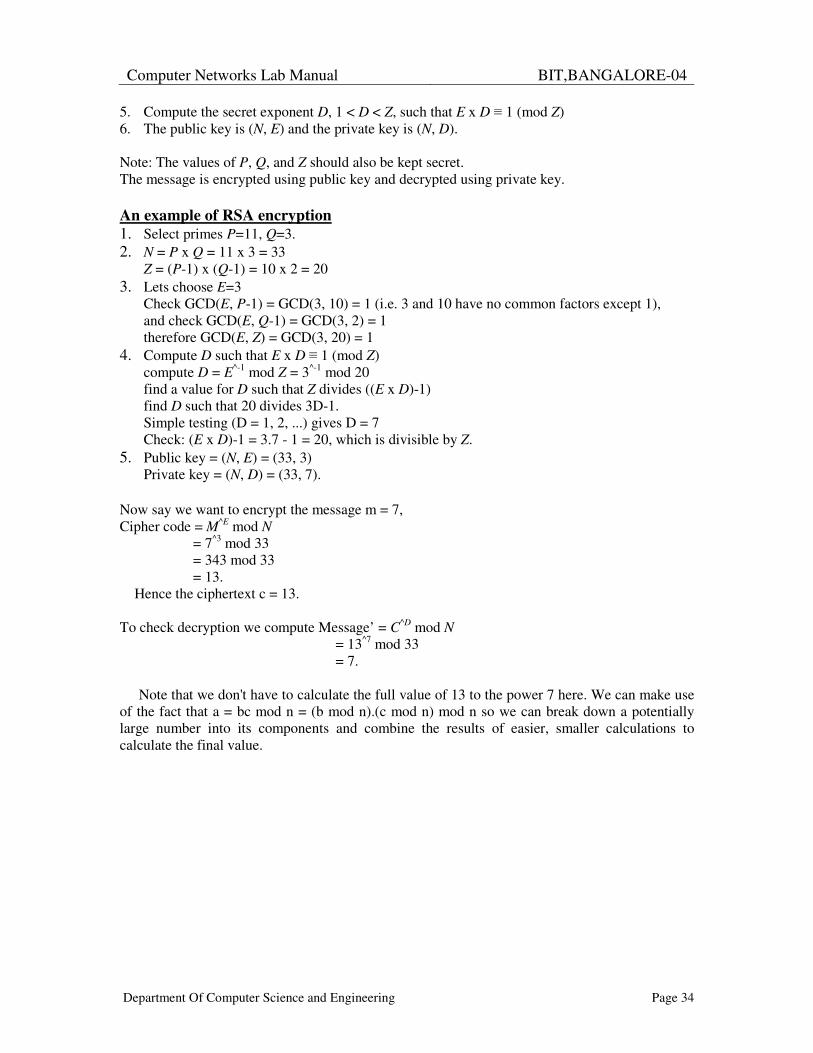
5. Compute the secret exponent D, 1 < D < Z, such that E x D � 1 (mod Z) 6. The public key is (N, E) and the private key is (N, D). Note: The values of P, Q, and Z should also be kept secret. The message is encrypted using public key and decrypted using private key. An example of RSA encryption 1. Select primes P=11, Q=3. 2. N = P x Q = 11 x 3 = 33

Z = (P-1) x (Q-1) = 10 x 2 = 20 3. Lets choose E=3

Check GCD(E, P-1) = GCD(3, 10) = 1 (i.e. 3 and 10 have no common factors except 1), and check GCD(E, Q-1) = GCD(3, 2) = 1 therefore GCD(E, Z) = GCD(3, 20) = 1

4. Compute D such that E x D � 1 (mod Z) compute D = E^-1 mod Z = 3^-1 mod 20 find a value for D such that Z divides ((E x D)-1) find D such that 20 divides 3D-1. Simple testing (D = 1, 2, ...) gives D = 7 Check: (E x D)-1 = 3.7 - 1 = 20, which is divisible by Z.

5. Public key = (N, E) = (33, 3) Private key = (N, D) = (33, 7).

Now say we want to encrypt the message m = 7, Cipher code = M^E mod N = 7^3 mod 33 = 343 mod 33 = 13. Hence the ciphertext c = 13. To check decryption we compute Message’ = C^D mod N = 13^7 mod 33 = 7.

Note that we don't have to calculate the full value of 13 to the power 7 here. We can make use of the fact that a = bc mod n = (b mod n).(c mod n) mod n so we can break down a potentially large number into its components and combine the results of easier, smaller calculations to calculate the final value.


BIT,BANGALORE-04


Experiment No 7 Hamming Codes

Problem Statement Write a program for Hamming Code generation for error detection and correction Theory

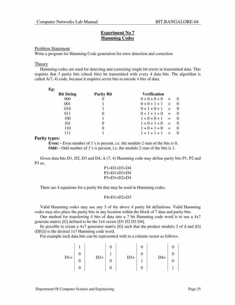
Hamming codes are used for detecting and correcting single bit errors in transmitted data. This requires that 3 parity bits (check bits) be transmitted with every 4 data bits. The algorithm is called A(7, 4) code, because it requires seven bits to encode 4 bits of data.

Eg: Bit String Parity Bit Verification

000 0 0 + 0 + 0 + 0 = 0 001 1 0 + 0 + 1 + 1 = 0 010 1 0 + 1 + 0 + 1 = 0 011 0 0 + 1 + 1 + 0 = 0 100 1 1 + 0 + 0 + 1 = 0 101 0 1 + 0 + 1 + 0 = 0 110 0 1 + 0 + 1 + 0 = 0 111 1 1 + 1 + 1 + 1 = 0

Parity types: Even: - Even number of 1’s is present, i.e. the modulo 2 sum of the bits is 0. Odd: - Odd number of 1’s is present, i.e. the modulo 2 sum of the bits is 1.

Given data bits D1, D2, D3 and D4, A (7, 4) Hamming code may define parity bits P1, P2 and

P3 as, P1=D2+D3+D4 P2=D1+D3+D4 P3=D1+D2+D4

There are 4 equations for a parity bit that may be used in Hamming codes,

P4=D1+D2+D3

Valid Hamming codes may use any 3 of the above 4 parity bit definitions. Valid Hamming

codes may also place the parity bits in any location within the block of 7 data and parity bits. One method for transferring 4 bits of data into a 7 bit Hamming code word is to use a 4x7

generate matrix [G] defined to be the 1x4 vector [D1 D2 D3 D4]. Its possible to create a 4x7 generator matrix [G] such that the product modulo 2 of d and [G]

(D[G]) is the desired 1x7 Hamming code word. For example each data bits can be represented with in a column vector as follows.

1 0 0 0

0 1 0 0

0 0 1 0 D1=

0

D2=

0

D3=

0

D4=

1


BIT,BANGALORE-04


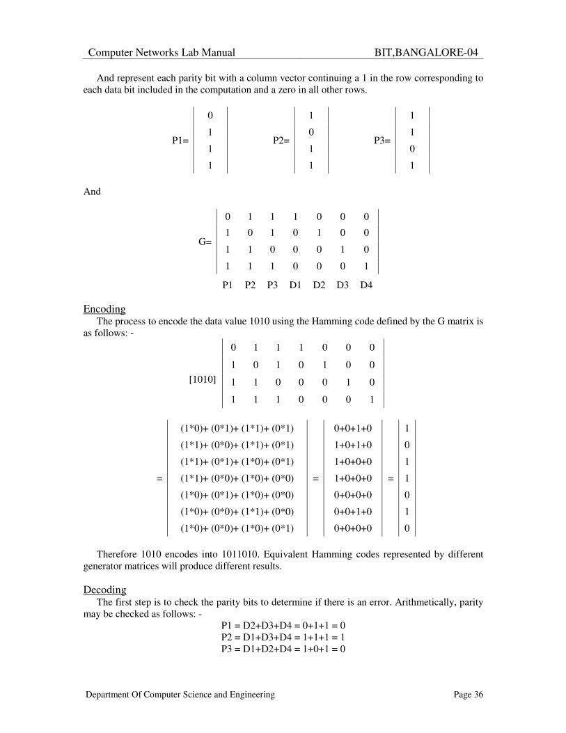
And represent each parity bit with a column vector continuing a 1 in the row corresponding to each data bit included in the computation and a zero in all other rows.

0 1 1

1 0 1

1 1 0 P1=

1

P2=

1

P3=

1 And

0 1 1 1 0 0 0

1 0 1 0 1 0 0

1 1 0 0 0 1 0 G=

1 1 1 0 0 0 1 P1 P2 P3 D1 D2 D3 D4

Encoding

The process to encode the data value 1010 using the Hamming code defined by the G matrix is as follows: -

0 1 1 1 0 0 0

1 0 1 0 1 0 0

1 1 0 0 0 1 0

[1010]

1 1 1 0 0 0 1

(1*0)+ (0*1)+ (1*1)+ (0*1) 0+0+1+0 1

(1*1)+ (0*0)+ (1*1)+ (0*1) 1+0+1+0 0

(1*1)+ (0*1)+ (1*0)+ (0*1) 1+0+0+0 1

(1*1)+ (0*0)+ (1*0)+ (0*0) 1+0+0+0 1

(1*0)+ (0*1)+ (1*0)+ (0*0) 0+0+0+0 0

(1*0)+ (0*0)+ (1*1)+ (0*0) 0+0+1+0 1

=

(1*0)+ (0*0)+ (1*0)+ (0*1)

=

0+0+0+0

=

0

Therefore 1010 encodes into 1011010. Equivalent Hamming codes represented by different generator matrices will produce different results. Decoding

The first step is to check the parity bits to determine if there is an error. Arithmetically, parity may be checked as follows: -

P1 = D2+D3+D4 = 0+1+1 = 0 P2 = D1+D3+D4 = 1+1+1 = 1 P3 = D1+D2+D4 = 1+0+1 = 0


BIT,BANGALORE-04


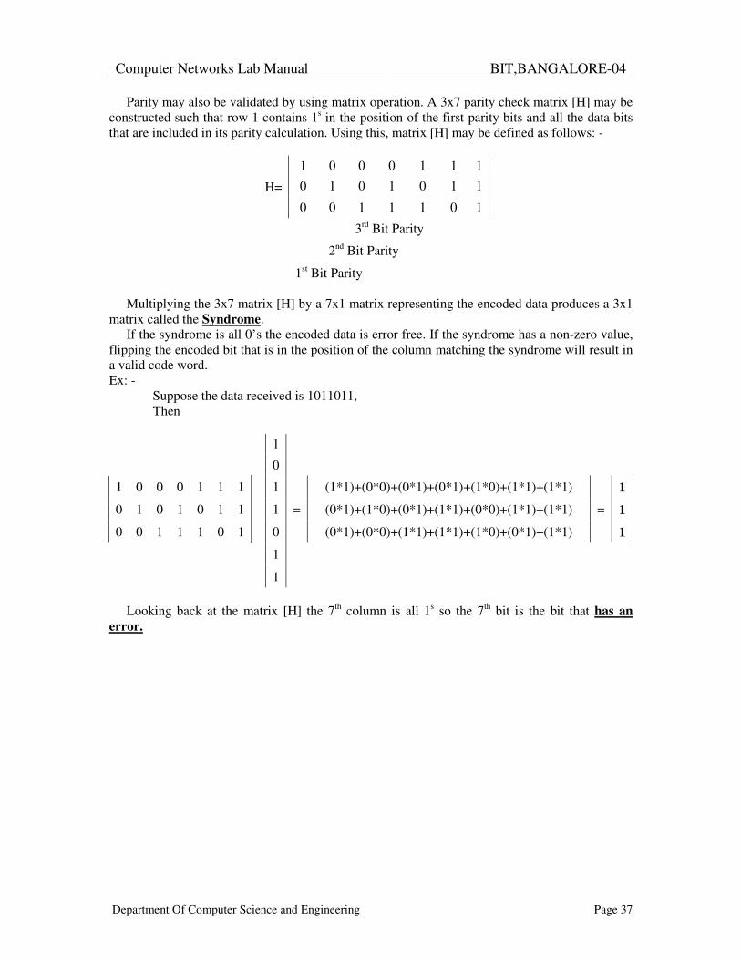
Parity may also be validated by using matrix operation. A 3x7 parity check matrix [H] may be constructed such that row 1 contains 1s in the position of the first parity bits and all the data bits that are included in its parity calculation. Using this, matrix [H] may be defined as follows: -

1 0 0 0 1 1 1

0 1 0 1 0 1 1 H=

0 0 1 1 1 0 1

3rd Bit Parity

2nd Bit Parity

1st Bit Parity

Multiplying the 3x7 matrix [H] by a 7x1 matrix representing the encoded data produces a 3x1 matrix called the Syndrome.

If the syndrome is all 0’s the encoded data is error free. If the syndrome has a non-zero value, flipping the encoded bit that is in the position of the column matching the syndrome will result in a valid code word. Ex: -

Suppose the data received is 1011011, Then

1

0

1 0 0 0 1 1 1 1 (1*1)+(0*0)+(0*1)+(0*1)+(1*0)+(1*1)+(1*1) 1

0 1 0 1 0 1 1 1 = (0*1)+(1*0)+(0*1)+(1*1)+(0*0)+(1*1)+(1*1) = 1

0 0 1 1 1 0 1 0 (0*1)+(0*0)+(1*1)+(1*1)+(1*0)+(0*1)+(1*1) 1

1

1

Looking back at the matrix [H] the 7th column is all 1s so the 7th bit is the bit that has an

error.


BIT,BANGALORE-04


Experiment No 8 Leaky Bucket

Problem Statement Write a program for congestion control using Leaky bucket algorithm. Theory

The congesting control algorithms are basically divided into two groups: open loop and closed loop. Open loop solutions attempt to solve the problem by good design, in essence, to make sure it does not occur in the first place. Once the system is up and running, midcourse corrections are not made. Open loop algorithms are further divided into ones that act at source versus ones that act at the destination.

In contrast, closed loop solutions are based on the concept of a feedback loop if there is any congestion. Closed loop algorithms are also divided into two sub categories: explicit feedback and implicit feedback. In explicit feedback algorithms, packets are sent back from the point of congestion to warn the source. In implicit algorithm, the source deduces the existence of congestion by making local observation, such as the time needed for acknowledgment to come back.

The presence of congestion means that the load is (temporarily) greater than the resources (in part of the system) can handle. For subnets that use virtual circuits internally, these methods can be used at the network layer.

Another open loop method to help manage congestion is forcing the packet to be transmitted at a more predictable rate. This approach to congestion management is widely used in ATM networks and is called traffic shaping.

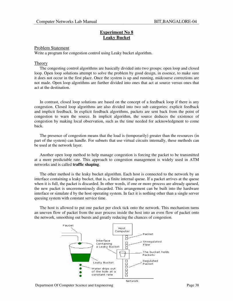
The other method is the leaky bucket algorithm. Each host is connected to the network by an interface containing a leaky bucket, that is, a finite internal queue. If a packet arrives at the queue when it is full, the packet is discarded. In other words, if one or more process are already queued, the new packet is unceremoniously discarded. This arrangement can be built into the hardware interface or simulate d by the host operating system. In fact it is nothing other than a single server queuing system with constant service time.

The host is allowed to put one packet per clock tick onto the network. This mechanism turns an uneven flow of packet from the user process inside the host into an even flow of packet onto the network, smoothing out bursts and greatly reducing the chances of congestion.

CN Lab Manual_algo

Documents

Transcript of CN Lab Manual_algo