Available on CMS information server CMS NOTE -2009/002

The Compact Muon Solenoid Experiment

Mailing address: CMS CERN, CH-1211 GENEVA 23, Switzerland

CMS Note

06 June 2008 (v6, 08 December 2008)

CMS Tracker Alignment at the Integration Facility

W. Adam, T. Bergauer, M. Dragicevic, M. Friedl, R. Fruhwirth, S. Hansel, J. Hrubec, M. Krammer, M.Oberegger,M. Pernicka, S. Schmid, R. Stark, H. Steininger, D. Uhl, W. Waltenberger, E. Widl

Institut fur Hochenergiephysik derOsterreichischen Akademie der Wissenschaften (HEPHY), Vienna, Austria

P. Van Mechelen, M. Cardaci, W. Beaumont, E. de Langhe, E. A. de Wolf, E. Delmeire, M. Hashemi

Universiteit Antwerpen, Belgium

O. Bouhali, O. Charaf, B. Clerbaux, J.-P. Dewulf. S. Elgammal, G. Hammad, G. de Lentdecker, P. Marage,C. Vander Velde, P. Vanlaer, J. Wickens

Universite Libre de Bruxelles, ULB, Bruxelles, Belgium

V. Adler, O. Devroede, S. De Weirdt, J. D’Hondt, R. Goorens, J. Heyninck, J. Maes, M. Mozer, S. Tavernier,L. Van Lancker, P. Van Mulders, I. Villella, C. Wastiels

Vrije Universiteit Brussel, VUB, Brussel, Belgium

J.-L. Bonnet, G. Bruno, B. De Callatay, B. Florins, A. Giammanco, G. Gregoire, Th. Keutgen, D. Kcira,V. Lemaitre, D. Michotte, O. Militaru, K. Piotrzkowski, L. Quertermont, V. Roberfroid, X. Rouby, D. Teyssier

Universite catholique de Louvain, UCL, Louvain-la-Neuve, Belgium

E. Daubie

Universite de Mons-Hainaut, Mons, Belgium

E. Anttila, S. Czellar, P. Engstrom, J. Harkonen, V. Karimaki, J. Kostesmaa, A. Kuronen, T. Lampen, T. Linden,P. -R. Luukka, T. Maenpaa, S. Michal, E. Tuominen, J. Tuominiemi

Helsinki Institute of Physics, Helsinki, Finland

M. Ageron, G. Baulieu, A. Bonnevaux, G. Boudoul, E. Chabanat, E. Chabert, R. Chierici, D. Contardo, R. DellaNegra, T. Dupasquier, G. Gelin, N. Giraud, G. Guillot, N. Estre, R. Haroutunian, N. Lumb, S. Perries, F. Schirra,

B. Trocme, S. Vanzetto

Universite de Lyon, Universite Claude Bernard Lyon 1, CNRS/IN2P3, Institut de Physique Nucleaire de Lyon, France

J.-L. Agram, R. Blaes, F. Drouhina), J.-P. Ernenwein, J.-C. Fontaine

Groupe de Recherches en Physique des Hautes Energies, Universite de Haute Alsace, Mulhouse, France

J.-D. Berst, J.-M. Brom, F. Didierjean, U. Goerlach, P. Graehling, L. Gross, J. Hosselet, P. Juillot, A. Lounis,C. Maazouzi, C. Olivetto, R. Strub, P. Van Hove

Institut Pluridisciplinaire Hubert Curien, Universite Louis Pasteur Strasbourg, IN2P3-CNRS, France

G. Anagnostou, R. Brauer, H. Esser, L. Feld, W. Karpinski, K. Klein, C. Kukulies, J. Olzem, A. Ostapchuk,D. Pandoulas, G. Pierschel, F. Raupach, S. Schael, G. Schwering, D. Sprenger, M. Thomas, M. Weber,

B. Wittmer, M. Wlochal

I. Physikalisches Institut, RWTH Aachen University, Germany

F. Beissel, E. Bock, G. Flugge, C. Gillissen, T. Hermanns, D. Heydhausen, D. Jahn, G. Kaussenb), A. Linn,L. Perchalla, M. Poettgens, O. Pooth, A. Stahl, M. H. Zoeller

III. Physikalisches Institut, RWTH Aachen University, Germany

P. Buhmann, E. Butz, G. Flucke, R. Hamdorf, J. Hauk, R. Klanner, U. Pein, P. Schleper, G. Steinbruck

University of Hamburg, Institute for Experimental Physics, Hamburg, Germany

P. Blum, W. De Boer, A. Dierlamm, G. Dirkes, M. Fahrer, M. Frey, A. Furgeri, F. Hartmanna), S. Heier,K.-H. Hoffmann, J. Kaminski, B. Ledermann, T. Liamsuwan, S. Muller, Th. Muller, F.-P. Schilling,

H.-J. Simonis, P. Steck, V. Zhukov

Karlsruhe-IEKP, Germany

P. Cariola, G. De Robertis, R. Ferorelli, L. Fiore, M. Preda,c), G. Sala, L. Silvestris, P. Tempesta, G. Zito

INFN Bari, Italy

D. Creanza, N. De Filippisd), M. De Palma, D. Giordano, G. Maggi, N. Manna, S. My, G. Selvaggi

INFN and Dipartimento Interateneo di Fisica, Bari, Italy

S. Albergo, M. Chiorboli, S. Costa, M. Galanti, N. Giudice, N. Guardone, F. Noto, R. Potenza, M. A. Saizuc),V. Sparti, C. Sutera, A. Tricomi, C. Tuve

INFN and University of Catania, Italy

M. Brianzi, C. Civinini, F. Maletta, F. Manolescu, M. Meschini, S. Paoletti, G. Sguazzoni

INFN Firenze, Italy

B. Broccolo, V. Ciulli, R. D’Alessandro. E. Focardi, S. Frosali, C. Genta, G. Landi, P. Lenzi, A. Macchiolo,N. Magini, G. Parrini, E. Scarlini

INFN and University of Firenze, Italy

G. Cerati

INFN and Universita degli Studi di Milano-Bicocca, Italy

P. Azzi, N. Bacchettaa), A. Candelori, T. Dorigo, A. Kaminsky, S. Karaevski, V. Khomenkovb), S. Reznikov,M. Tessaro

INFN Padova, Italy

D. Bisello, M. De Mattia, P. Giubilato, M. Loreti, S. Mattiazzo, M. Nigro, A. Paccagnella, D. Pantano,N. Pozzobon, M. Tosi

INFN and University of Padova, Italy

G. M. Bileia), B. Checcucci, L. Fano, L. Servoli

INFN Perugia, Italy

F. Ambroglini, E. Babucci, D. Benedettie), M. Biasini, B. Caponeri, R. Covarelli, M. Giorgi, P. Lariccia,G. Mantovani, M. Marcantonini, V. Postolache, A. Santocchia, D. Spiga

INFN and University of Perugia, Italy

G. Bagliesi , G. Balestri, L. Berretta, S. Bianucci, T. Boccali, F. Bosi, F. Bracci, R. Castaldi, M. Ceccanti,R. Cecchi, C. Cerri, A .S. Cucoanes, R. Dell’Orso, D .Dobur, S .Dutta, A. Giassi, S. Giusti, D. Kartashov,

A. Kraan, T. Lomtadze, G. A. Lungu, G. Magazzu, P. Mammini, F. Mariani, G. Martinelli, A. Moggi, F. Palla,F. Palmonari, G. Petragnani, A. Profeti, F. Raffaelli, D. Rizzi, G. Sanguinetti, S. Sarkar, D. Sentenac, A. T. Serban,

A. Slav, A. Soldani, P. Spagnolo, R. Tenchini, S. Tolaini, A. Venturi, P. G. Verdinia), M. Vosf), L. Zaccarelli

INFN Pisa, Italy

C. Avanzini, A. Basti, L. Benuccig), A. Bocci, U. Cazzola, F. Fiori, S. Linari, M. Massa, A. Messineo, G. Segneri,G. Tonelli

University of Pisa and INFN Pisa, Italy

P. Azzurri, J. Bernardini, L. Borrello, F. Calzolari, L. Foa, S. Gennai, F. Ligabue, G. Petrucciani , A. Rizzih),Z. Yangi)

Scuola Normale Superiore di Pisa and INFN Pisa, Italy

F. Benotto, N. Demaria, F. Dumitrache, R. Farano

INFN Torino, Italy

M.A. Borgia, R. Castello, M. Costa, E. Migliore, A. Romero

INFN and University of Torino, Italy

D. Abbaneo, M. Abbas,I. Ahmed, I. Akhtar, E. Albert, C. Bloch, H. Breuker, S. Butt,O. Buchmullerj), A. Cattai,C. Delaerek), M. Delattre,L. M. Edera, P. Engstrom, M. Eppard, M. Gateau, K. Gill, A.-S. Giolo-Nicollerat,R. Grabit, A. Honma, M. Huhtinen, K. Kloukinas, J. Kortesmaa, L. J. Kottelat, A. Kuronen, N. Leonardo,

C. Ljuslin, M. Mannelli, L. Masetti, A. Marchioro, S. Mersi, S. Michal, L. Mirabito, J. Muffat-Joly, A. Onnela,C. Paillard, I. Pal, J. F. Pernot, P. Petagna, P. Petit, C. Piccut, M. Pioppi, H. Postema, R. Ranieri, D. Ricci,G. Rolandi, F. Rongal), C. Sigaud, A. Syed, P. Siegrist, P. Tropea, J. Troska, A. Tsirou, M. Vander Donckt,

F. Vasey

European Organization for Nuclear Research (CERN), Geneva, Switzerland

E. Alagoz, C. Amsler, V. Chiochia, C. Regenfus, P. Robmann, J. Rochet, T. Rommerskirchen, A. Schmidt,S. Steiner, L. Wilke

University of Zurich, Switzerland

I. Church, J. Colen), J. Coughlan, A. Gay, S. Taghavi, I. Tomalin

STFC, Rutherford Appleton Laboratory, Chilton, Didcot, United Kingdom

R. Bainbridge, N. Cripps, J. Fulcher, G. Hall, M. Noy, M. Pesaresi, V. Radiccin), D. M. Raymond, P. Sharpa),M. Stoye, M. Wingham, O. Zorba

Imperial College, London, United Kingdom

I. Goitom, P. R. Hobson, I. Reid, L. Teodorescu

Brunel University, Uxbridge, United Kingdom

G. Hanson, G.-Y. Jeng, H. Liu, G. Pasztoro), A. Satpathy, R. Stringer

University of California, Riverside, California, USA

B. Mangano

University of California, San Diego, California, USA

K. Affolder, T. Affolderp), A. Allen, D. Barge, S. Burke, D. Callahan, C. Campagnari, A. Crook, M. D’Alfonso,J. Dietch, J. Garberson, D. Hale, H. Incandela, J. Incandela, S. Jaditzq), P. Kalavase, S. Kreyer, S. Kyre, J. Lamb,

C. Mc Guinnessr), C. Millss), H. Nguyen, M. Nikolicm), S. Lowette, F. Rebassoo, J. Ribnik, J. Richman,N. Rubinstein, S. Sanhueza, Y. Shah, L. Simmsr), D. Staszakt), J. Stoner, D. Stuart, S. Swain, J.-R. Vlimant,

D. White

University of California, Santa Barbara, California, USA

K. A. Ulmer, S. R. Wagner

University of Colorado, Boulder, Colorado, USA

L. Bagby, P. C. Bhat, K. Burkett, S. Cihangir, O. Gutsche, H. Jensen, M. Johnson, N. Luzhetskiy, D. Mason,T. Miao, S. Moccia, C. Noeding, A. Ronzhin, E. Skup, W. J. Spalding, L. Spiegel, S. Tkaczyk, F. Yumiceva,

A. Zatserklyaniy, E. Zerev

Fermi National Accelerator Laboratory (FNAL), Batavia, Illinois, USA

I. Anghel, V. E. Bazterra, C. E. Gerber, S. Khalatian, E. Shabalina

University of Illinois, Chicago, Illinois, USA

P. Baringer, A. Bean, J. Chen, C. Hinchey, C. Martin,T. Moulik, R. Robinson

University of Kansas, Lawrence, Kansas, USA

A. V. Gritsan, C. K. Lae, N. V. Tran

Johns Hopkins University, Baltimore, Maryland, USA

P. Everaerts, K. A. Hahn, P. Harris, S. Nahn, M. Rudolph, K. Sung

Massachusetts Institute of Technology, Cambridge, Massachusetts, USA

B. Betchart, R. Demina, Y. Gotra, S. Korjenevski, D. Miner, D. Orbaker

University of Rochester, New York, USA

L. Christofek, R. Hooper, G. Landsberg, D. Nguyen, M. Narain,T. Speer, K. V. Tsang

Brown University, Providence, Rhode Island, USA

a) Also at CERN, European Organization for Nuclear Research, Geneva, Switzerlandb) Now at University of Hamburg, Institute for Experimental Physics, Hamburg, Germanyc) On leave from IFIN-HH, Bucharest, Romaniad) Now at LLR-Ecole Polytechnique, Francee) Now at Northeastern University, Boston, USAf) Now at IFIC, Centro mixto U. Valencia/CSIC, Valencia, Spaing) Now at Universiteit Antwerpen, Antwerpen, Belgiumh) Now at ETH Zurich, Zurich, Switzerlandi) Also Peking University, Chinaj) Now at Imperial College, London, UKk) Now at Universite catholique de Louvain, UCL, Louvain-la-Neuve, Belgiuml) Now at Eidgenossische Technische Hochschule, Zurich, Switzerland

m) Now at University of California, Davis, California, USAn) Now at Kansas University, USAo) Also at Research Institute for Particle and Nuclear Physics, Budapest, Hungaryp) Now at University of Liverpool, UKq) Now at Massachusetts Institute of Technology, Cambridge, Massachusetts, USAr) Now at Stanford University, Stanford, California, USAs) Now at Harvard University, Cambridge, Massachusetts, USAt) Now at University of California, Los Angeles, California, USA

Abstract

The results of the CMS tracker alignment analysis are presented using the data from cosmic tracks, op-tical survey information, and the laser alignment system at the Tracker Integration Facility at CERN.During several months of operation in the spring and summer of 2007, about five million cosmic trackevents were collected with a partially active CMS Tracker. This allowed us to perform first alignmentof the active silicon modules with the cosmic tracks using three different statistical approaches; val-idate the survey and laser alignment system performance; and test the stability of Tracker structuresunder various stresses and temperatures ranging from+15◦C to−15◦C. Comparison with simulationshows that the achieved alignment precision in the barrel part of the tracker leads to residual distribu-tions similar to those obtained with a random misalignment of50 (80) µm in the outer (inner) part ofthe barrel.

Contents

1 Introduction 2

1.1 TIF Tracker and Goal of Alignment . . . . . . . . . . . . . . . . . . . .. . . . . . . . . . . . . 2

1.2 CMS Tracker Geometry . . . . . . . . . . . . . . . . . . . . . . . . . . . . . .. . . . . . . . . . 2

2 Input to Alignment 3

2.1 Data Samples, Tracking, and Event Selection . . . . . . . . . .. . . . . . . . . . . . . . . . . . 3

2.2 Survey of the CMS Tracker . . . . . . . . . . . . . . . . . . . . . . . . . . .. . . . . . . . . . . 5

2.3 Laser Alignment System of the CMS Tracker . . . . . . . . . . . . .. . . . . . . . . . . . . . . 6

3 Statistical Methods and Approaches 7

3.1 Alignment Concepts . . . . . . . . . . . . . . . . . . . . . . . . . . . . . . .. . . . . . . . . . 7

3.1.1 HIP algorithm . . . . . . . . . . . . . . . . . . . . . . . . . . . . . . . . . .. . . . . . 7

3.1.2 Kalman filter algorithm . . . . . . . . . . . . . . . . . . . . . . . . . .. . . . . . . . . . 8

3.1.3 Millepede algorithm . . . . . . . . . . . . . . . . . . . . . . . . . . . .. . . . . . . . . 8

3.1.4 Limitations of alignment algorithms . . . . . . . . . . . . . .. . . . . . . . . . . . . . . 9

3.2 Application of Alignment Algorithms to the TIF Analysis. . . . . . . . . . . . . . . . . . . . . . 9

3.2.1 HIP algorithm . . . . . . . . . . . . . . . . . . . . . . . . . . . . . . . . . .. . . . . . 10

3.2.2 Kalman filter algorithm . . . . . . . . . . . . . . . . . . . . . . . . . .. . . . . . . . . . 11

3.2.3 Millepede algorithm . . . . . . . . . . . . . . . . . . . . . . . . . . . .. . . . . . . . . 11

4 Validation of Alignment of the CMS Tracker at TIF 14

4.1 Validation Methods . . . . . . . . . . . . . . . . . . . . . . . . . . . . . . .. . . . . . . . . . . 14

4.2 Validation of the Assembly and Survey Precision . . . . . . .. . . . . . . . . . . . . . . . . . . 15

4.3 Validation of the Track-Based Alignment . . . . . . . . . . . . .. . . . . . . . . . . . . . . . . 17

4.4 Geometry comparisons . . . . . . . . . . . . . . . . . . . . . . . . . . . . .. . . . . . . . . . . 21

4.5 Track-Based Alignment with Simulated Data and Estimation of Alignment Precision . . . . . . . 21

5 Stability of the Tracker Geometry with Temperature and Time 24

5.1 Stability of the Tracker Barrels . . . . . . . . . . . . . . . . . . . .. . . . . . . . . . . . . . . . 24

5.2 Stability of the Tracker Endcap . . . . . . . . . . . . . . . . . . . . .. . . . . . . . . . . . . . . 28

6 Laser Alignment System Analysis and Discussion 28

6.1 Data Taking . . . . . . . . . . . . . . . . . . . . . . . . . . . . . . . . . . . . . .. . . . . . . . 28

6.2 Results from Alignment Tubes . . . . . . . . . . . . . . . . . . . . . . .. . . . . . . . . . . . . 29

6.3 Comparison of LAS and Track Based Alignment Results . . . .. . . . . . . . . . . . . . . . . . 29

7 Summary and Conclusion 29

8 Acknowledgments 32

1

1 IntroductionThe all-silicon design of the CMS tracker poses new challenges in aligning a system with more than 15,000independent modules. It is necessary to understand the alignment of the silicon modules to close to a few micronprecision. Given the inaccessibility of the interaction region, the most accurate way to determine the silicondetector positions is to use the data generated by the silicon detectors themselves when they are traversed in-situby charged particles. Additional information about the module positions is provided by the optical survey duringconstruction and by the Laser Alignment System during the detector operation.

1.1 TIF Tracker and Goal of Alignment

A unique opportunity to gain experience in alignment of the CMS silicon strip tracker [1, 2] ahead of the installationat the underground cavern comes from tests performed at the Tracker Integration Facility (TIF). During severalmonths of operation in the spring and summer of 2007, about five million cosmic track events were collected totape. The tracker was operated with different coolant temperatures ranging from+15◦C to−15◦C. About 15% ofthe silicon strip tracker was powered and read-out simultaneously. An external trigger system was used to triggeron cosmic track events. The silicon pixel detector was only trial-inserted at TIF and was not involved in datataking.

In this note, we show alignment results primarily with the track-based approach, where three statistical algorithmshave been employed showing consistent results. Assembly precision and structure stability with time are alsostudied. The experience gained in analysis of the TIF data will help evolving alignment strategies with tracks, giveinput into the stability of the detector components with temperature and assembly progress, and test the reliabilityof the optical survey information and the laser alignment system in anticipation of the first LHC beam collisions.

1.2 CMS Tracker Geometry

The CMS tracker is the largest silicon detector ever constructed. Even with about 15% of the silicon strip trackeractivated during the TIF test, more than 2,000 individual modules were read out.

The strip detector of CMS is composed of four sub-detectors,as sketched in Fig. 1: the Tracker Inner and OuterBarrels (TIB and TOB), the Tracker Inner Disks (TID), and theTracker Endcaps (TEC). They are all concentricallyarranged around the nominal LHC beam axis that coincides with thez-axis. The right handed, orthogonal CMScoordinate system is completed by thex- andy-axes where the latter is pointing upwards. The polar and azimuthalanglesφ andθ are measured from the positivex- andz-axis, respectively, whereas the radiusr denotes the distancefrom thez-axis.

Figure 1:A quarter of the CMS silicon tracker in anrz view. Single module positions are indicated as purple linesand dark blue lines indicate pairs ofrφ and stereo modules. The path of the laser rays, the beam splitters (BS) andthe alignment tubes (AT) of the Laser Alignment System are shown.

The TIB and TOB are composed of four and six layers, respectively. Modules are arranged in linear structuresparallel to thez-axis, which are named “strings” for TIB (each containing three modules) and “rods” for TOB(each containing six modules). The TID has six identical disk structures. The modules are arranged on both sidesof ring-shaped concentric structures, numbering three perdisk. Both TECs are built from nine disks, with eight

2

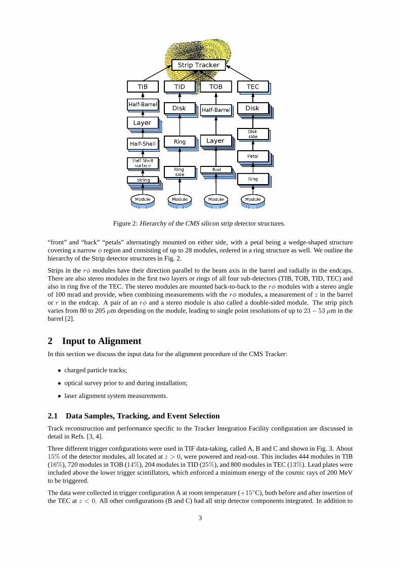
Figure 2:Hierarchy of the CMS silicon strip detector structures.

“front” and “back” “petals” alternatingly mounted on either side, with a petal being a wedge-shaped structurecovering a narrowφ region and consisting of up to 28 modules, ordered in a ring structure as well. We outline thehierarchy of the Strip detector structures in Fig. 2.

Strips in therφ modules have their direction parallel to the beam axis in thebarrel and radially in the endcaps.There are also stereo modules in the first two layers or rings of all four sub-detectors (TIB, TOB, TID, TEC) andalso in ring five of the TEC. The stereo modules are mounted back-to-back to therφ modules with a stereo angleof 100 mrad and provide, when combining measurements with the rφ modules, a measurement ofz in the barrelor r in the endcap. A pair of anrφ and a stereo module is also called a double-sided module. Thestrip pitchvaries from 80 to 205µm depending on the module, leading to single point resolutions of up to23− 53 µm in thebarrel [2].

2 Input to AlignmentIn this section we discuss the input data for the alignment procedure of the CMS Tracker:

• charged particle tracks;

• optical survey prior to and during installation;

• laser alignment system measurements.

2.1 Data Samples, Tracking, and Event Selection

Track reconstruction and performance specific to the Tracker Integration Facility configuration are discussed indetail in Refs. [3, 4].

Three different trigger configurations were used in TIF data-taking, called A, B and C and shown in Fig. 3. About15% of the detector modules, all located atz > 0, were powered and read-out. This includes 444 modules in TIB(16%), 720 modules in TOB (14%), 204 modules in TID (25%), and 800 modules in TEC (13%). Lead plates wereincluded above the lower trigger scintillators, which enforced a minimum energy of the cosmic rays of 200 MeVto be triggered.

The data were collected in trigger configuration A at room temperature (+15◦C), both before and after insertion ofthe TEC atz < 0. All other configurations (B and C) had all strip detector components integrated. In addition to

3

Figure 3:Layout of the CMS Strip Tracker and of the trigger scintillators at TIF. The acceptance region is indicatedby the straight lines connecting the active areas of the scintillators. Configuration A corresponds approximatelyto the acceptance region defined by the forward (right) bottom scintillator; configuration B corresponds to the leftbottom scintillator; and configuration C combines both of the above.

Label TriggerPosition

Temperature Ntrig

A1 A 15◦C 665 409 before TEC- insertionA2 A 15◦C 189 925 after TEC- insertion

B B 15◦C 177 768

C15 C 15◦C 129 378C10 C 10◦C 534 759C0 C -1◦C 886 801

C−10 C -10◦C 902 881C−15 C -15◦C 655 301 less modules read outC14 C 14◦C 112 134

MC C – 3 091 306 simulation

Table 1:Overview of different data sets, ordered in time, and their number of triggered eventsNtrig taking intoaccount only good running conditions.

room temperature, configuration C was operated at +10◦C, -1◦C, -10◦C, and -15◦C. Due to cooling limitations,a large number of modules had to be turned off at -15◦C. The variety of different configurations allows us to studyalignment stability with different stress and temperatureconditions. Table 1 gives an overview of the different datasets.

We also validate tracking and alignment algorithm performances with simulation. A sample of approximatelythree million cosmic track events was simulated using the CMSCGEN simulator [5]. Only cosmic muon trackswithin specific geometrical ranges were selected to simulate the scintillator trigger configuration C. To extendCMSCGEN’s energy range, events at low muon energy have been re-weighted to adjust the energy spectrum to theCAPRICE data [6].

Charged track reconstruction includes three essential steps: seed finding, pattern recognition, and track fitting. Sev-eral pattern recognition algorithms are employed on CMS, such as “Combinatorial Track Finder” (CTF), “RoadSearch”, and “Cosmic Track Finder”, the latter being specific to the cosmic track reconstruction. All three algo-rithms use the Kalman filter algorithm for final track fitting,but the first two steps are different. The track modelused is a straight line parametrised by four parameters where the Kalman filter track fit includes multiple scatteringeffects in each crossed layer. We employ the CTF algorithm for alignment studies in this note.

In order to recover tracking efficiency which is otherwise lost in the pattern recognition phase because hits aremoved outside the standard search window defined by the detector resolution, an “alignment position error” (APE)is introduced. This APE is added quadratically to the hit resolution, and the combined value is subsequently usedas a search window in the pattern recognition step. The APE settings used for the TIF data are modelling theassembly tolerances [2].

4

There are several important aspects of the TIF configurationwhich require special handling with respect to normaldata-taking. First of all, no magnetic field is present. Therefore, the momentum of the tracks cannot be measuredand estimates of the energy loss and multiple scattering canbe done only approximately. A track momentum of1 GeV/c is assumed in the estimates, which is close to the average cosmic track momentum observed in simulatedspectra. Other TIF-specific features are due to the fact thatthe cosmic muons do not originate from the interactionregion. Therefore the standard seeding mechanism is extended to use also hits in the TOB and TEC, and no beamspot constraint is applied. For more details see Ref. [3].

Reconstruction of exactly one cosmic muon track in the eventis required. A number of selection criteria is appliedon the hits, tracks, and detector components subject to alignment, to ensure good quality data. This is done based ontrajectory estimates and the fiducial tracking geometry. Inaddition, hits from noisy clusters or from combinatorialbackground tracks are suppressed by quality cuts on the clusters. The detailed track selection is as follows:

• The direction of the track trajectory satisfies the requirements:−1.5 < ηtrack < 0.6 and−1.8 < φtrack <−1.2 rad, according to the fiducial scintillator positions.

• Theχ2 value of the track fit, normalised to the number of degrees of freedom, fulfilsχ2track/ndof< 4.

• The track has at least 5 hits associated and among those at least 2 matched hits in double-sided modules.

A hit is kept for the track fit:

• If it is associated to a cluster with a total charge of at least50 ADC counts. If the hit is matched, bothcomponents must satisfy this requirement.

• If it is isolated, i.e. if any other reconstructed hit is found on the same module within 8.0 mm, the wholetrack is rejected. This cut helps in rejecting fake clustersgenerated by noisy strips and modules.

• If it is not discarded by the outlier rejection step during the refit (see below).

The remaining tracks and their associated hits are refit in every iteration of the alignment algorithms. An outlierrejection technique is applied during the refit. Its principle is to iterate the final track fit until no outliers are found.An outlier is defined as a hit whose trajectory estimate is larger than a given cut value (ecut = 5). The trajectoryestimate of a hit is the quantity:e = rT · V−1 · r, wherer is the 1- or 2-dimensional local residual vector andV

is the associated covariance matrix. If one or more outliersare found in the first track fit, they are removed fromthe hit collection and the fit is repeated. This procedure is iterated until there are no more outliers or the numberof surviving hits is less than 4.

Unless otherwise specified, these cuts are common to all alignment algorithms used. The combined efficiency forall the cuts above is estimated to be 8.3% on TIF data (theC−10 sample is used in this estimate) and 20.5% in theTIF simulation sample.

2.2 Survey of the CMS Tracker

Information about the relative position of modules within detector components and of the larger-level structureswithin the tracker is available from the optical survey analysis prior to or during the tracker integration. Thisincludes Coordinate Measuring Machine (CMM) data and photogrammetry, the former usually used for the activeelement measurements and the latter for the larger object alignment. For the inner strip detectors (TIB and TID),survey data at all levels was used in analysis. For the outer strip detectors (TOB and TEC), module-level surveywas used only for mounting precision monitoring, while survey of high-level structures was used in analysis.

For TIB, survey measurements are available for the module positions with respect to shells, and of cylinders withrespect to the tracker support tube. Similarly, for TID, survey measurements were done for modules with respectto the rings, rings with respect to the disks and disks with respect to the tracker support tube. For TOB, the wheelwas measured with respect to the tracker support tube. For TEC, measurements are stored at the level of disks withrespect to the endcaps and endcaps with respect to the tracker support tube.

Figure 4 illustrates the relative positions of the CMS tracker modules with respect to design geometry as measuredin optical survey: as can be seen, differences from design geometry as large as several millimetres are expected.Since hierarchical survey measurements were performed andTOB and TEC have only large-structure information,the corresponding modules appear to be coherently displaced in the plot.

5

Figure 4:Displacement of modules in global cylindrical coordinatesas measured in survey with respect to designgeometry. A colour coding is used: black for TIB, green for TID, red for TOB, and blue for TEC.

2.3 Laser Alignment System of the CMS Tracker

The Laser Alignment System (LAS) uses infrared laser beams with a wavelength ofλ = 1075nm to monitor theposition of selected tracker modules. It operates globallyon tracker substructures (TIB, TOB and TEC disks) andcannot determine the position of individual modules. The goal of the system, already sketched in Fig. 1, is to gen-erate alignment information on a continuous basis, providing geometry reconstruction of the tracker substructuresat the level of100µm. In addition, possible tracker structure movements can bemonitored at the level of10 µm,providing additional input for the track based alignment.

In each TEC, laser beams cross all nine TEC disks in ring 6 and ring 4 on the back petals, equally distributed inφ. Here, special silicon sensors with a10 mm hole in the backside metallisation and an anti-reflectivecoating aremounted. The beams are used for the internal alignment of theTEC disks. The other eight beams, distributedin φ, are foreseen to align TIB, TOB, and both TECs with respect toeach other. Finally, there is a link to themuon system, which is established by 12 laser beams (six on each side) with precise position and orientation in thetracker coordinate system.

The signal induced by the laser beams on the silicon sensors decreases in height as the beams penetrate throughsubsequent silicon layers in the TECs and through beam splitters in the alignment tubes that partly deflect thebeams onto TIB and TOB sensors. To obtain optimal signals on all sensors, a sequence of laser pulses withincreasing intensities, optimised for each position, is generated. Several triggers per intensity are taken and thesignals are averaged. In total, a few hundred triggers are needed to get a full picture of the alignment of the trackerstructure. Since the trigger rate for the alignment system is around100Hz, this takes only a few seconds.

6

3 Statistical Methods and ApproachesAll the methods use a common definition of module coordinatesfor alignment. A module is assumed to be a rigidbody, so three absolute positions and three rotations are sufficient to express its degrees of freedom, illustrated inFig. 5. Thus, the final goal of the alignment procedure is to obtain six parameters for each independent module,these being the three spatial and three rotational parameters.

w ( r)

u ( rφ)v ( z)

αγβ

+

++

Figure 5: Schematic illustration of the local coordinates of a module as used for alignment. Global parameters (inparentheses) are shown for modules in the barrel detectors (TIB and TOB).

The local positions are calledu, v andw, whereu is along the sensitive coordinate (i.e. across the strips),vis perpendicular tou in the sensor plane andw is perpendicular to theuv-plane, completing the right-handedcoordinate system. The rotations around theu, v andw axes are calledα, β andγ, respectively. In the case ofalignment of intermediate structures like rods, strings orpetals, we follow the convention thatu andv are paralleland perpendicular to the precisely measured coordinate, while for the large structures like layers and disks, thelocal coordinates coincide with the global ones.

3.1 Alignment Concepts

Alignment analysis with tracks uses the fact that the hit positions and the measured trajectory impact points of atrack are systematically displaced if the module position is not known correctly. The difference in local modulecoordinates between these two quantities are thetrack-hit residuals ri, which are 1- (2-dimensional) vectors in thecase of a single (double) sided module and which one would like to minimise. More precisely, one can minimisetheχ2 function which includes a covariance matrixV of the measurement uncertainties:

χ2 =

hits∑

i

rTi (p,q)V−1

i ri(p,q) (1)

wherep represents the position and orientation of the modules andq represents the track parameters.

There are different alignment methods used to minimise Eq. (1). It can be solved either directly or by minimisingsubsets of the parameters (a local method, e.g. per module) over iterations. In this section, we discuss the threestatistical methods used for track-based alignment in thisanalysis.

• Hits and Impact Points (HIP) local iterative method;

• Kalman filter fit method;

• Millepede global minimisation method.

3.1.1 HIP algorithm

The HIP (Hits and Impact Points) algorithm is described in detail in Ref. [7], where its application to the pixeldetectors with simulated collision data is studied. The solution of theχ2 minimisation in Eq. (1) can be found in thegeneral formalism with the linear approximation for the alignment parameterspm of each module independently:

pm =

[

hits∑

i

JTi V−1

i Ji

]−1 [

hits∑

i

JTi V−1

i ri

]

(2)

where the JacobianJi is defined as the derivative of the residual with respect to the sensor position parameters andcan be found analytically. The Jacobian is a matrixN × 6, whereN is the residual dimension. In the case of 1Dor 2D track-hit residualsri, the JacobianJi can be computed with the small angle approximation. Correlationsbetween different modules and effects on the track parameters are neglected in Eq. (2). They are accounted for byiterating the minimisation process and by refitting the tracks with new alignment constants after each iteration.

7

3.1.2 Kalman filter algorithm

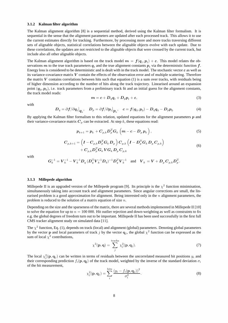
The Kalman alignment algorithm [8] is a sequential method, derived using the Kalman filter formalism. It issequential in the sense that the alignment parameters are updated after each processed track. This allows it to usethe current estimates directly for tracking. Furthermore,by processing more and more tracks traversing differentsets of alignable objects, statistical correlations between the alignable objects evolve with each update. Due tothese correlations, the updates are not restricted to the alignable objects that were crossed by the current track, butinclude also all other alignable objects.

The Kalman alignment algorithm is based on the track modelm = f (qt,pt) + ε. This model relates the ob-servationsm to the true track parametersqt and the true alignment constantspt via the deterministic functionf .Energy loss is considered to be deterministic and is dealt with in the track model. The stochastic vectorε as well asits variance-covariance matrixV contain the effects of the observation error and of multiplescattering. Thereforethe matrixV contains correlations between hits such that equation (1) is a sum over tracks, with residuals beingof higher dimension according to the number of hits along thetrack trajectory. Linearised around an expansionpoint (q0,p0), i.e. track parameters from a preliminary track fit and an initial guess for the alignment constants,the track model reads:

m = c + Dqqt + Dppt + ε, (3)

withDq = ∂f/∂qt

∣

∣

q0

, Dp = ∂f/∂pt

∣

∣

p0

, c = f (q0,p0) − Dqq0 − Dpp0 (4)

By applying the Kalman filter formalism to this relation, updated equations for the alignment parametersp andtheir variance-covariance matrixCp can be extracted. At stepk, these equations read:

pk+1 = pk + Cp,kDTp Gk

(

m − c − Dp pk

)

, (5)

Cp,k+1 =(

I − Cp,kDTp Gk Dp

)

Cp,k

(

I − DTp Gk Dp Cp,k

)

+ Cp,kDTp Gk V Gk Dp Cp,k

(6)

withG−1

k = V −1

k − V −1

k Dq (DTq V −1

k Dq)−1DT

q V −1

k and V k = V + Dp Cp,kDTp .

3.1.3 Millepede algorithm

Millepede II is an upgraded version of the Millepede program[9]. Its principle is theχ2 function minimisation,simultaneously taking into account track and alignment parameters. Since angular corrections are small, the lin-earised problem is a good approximation for alignment. Being interested only in then alignment parameters, theproblem is reduced to the solution of a matrix equation of sizen.

Depending on the size and the sparseness of the matrix, thereare several methods implemented in Millepede II [10]to solve the equation for up ton = 100 000. Hit outlier rejection and down-weighting as well asconstraints to fixe.g. the global degrees of freedom turn out to be important. Millepede II has been used successfully in the first fullCMS tracker alignment study on simulated data [11].

Theχ2 function, Eq. (1), depends on track (local) and alignment (global) parameters. Denoting global parametersby the vectorp and local parameters of trackj by the vectorqj , the globalχ2 function can be expressed as thesum of localχ2 contributions,

χ2(p,q) =

tracks∑

j

χ2j(p,qj). (7)

The localχ2j(p,qj) can be written in terms of residuals between the uncorrelated measured hit positionsyi and

their corresponding predictionfi(p,qj) of the track model, weighted by the inverse of the standard deviationσi

of the hit measurement,

χ2j(p,qj) =

hits∑

i

(yi − fi(p,qj))2

σ2i

. (8)

8

Given reasonable start valuesp0 andqj0 as expected in alignment, the track model predictionfi(p,qj) can belinearised. Equation 8 becomes

χ2j(p,qj) ≈

hits∑

i

(

yi − fi(p0,qj0) + ∂fi

∂pa + ∂fi

∂qj∆qj

)2

σ2i

, (9)

where the alignment parametersa = ∆p denote the small correction to the global parameters and∆qj the correc-tion to the local parameters.

Using this linearision,∑

j χ2j can be minimised using the least squares method. This results in a large linear

system with one equation for each alignment parameter and all the track parameters of each track. But since theparameterisation of a trackk is independent of the parameters of trackj (∂fk

i /∂qj = 0, k 6= j), the particularstructure of the system of equations allows a reduction of its size, leading to a matrix equation

Ca = b, (10)

where the matrixC is built from the derivatives∂fi/∂qj and∂fi/∂p and the vectorb from the derivatives andthe residuals(yi − fi(p0,qj0)), all normalised to the uncertaintiesσi.

3.1.4 Limitations of alignment algorithms

We should note that Eq. (1) may be invariant under certain coherent transformations of assumed module positions,the so-called “weak” modes. The trivial transformation which isχ2-invariant is a global translation and rotation ofthe whole tracker. This transformation has no effect in internal alignment, and is easily resolved by a suitable con-vention for defining the global reference frame. Different algorithms employ different approaches and conventionshere, so we will discuss this in more detail as it applies to each algorithm.

The non-trivialχ2-invariant transformations which preserve Eq. (1) are of larger concern. For the full CMS trackerwith cylindrical symmetry one could define certain “weak” modes, such as elliptical distortion, twist, etc., de-pending on the track sample used. However, since we use only apartial CMS tracker without the full azimuthalcoverage, different “weak” modes may show up. For example, since we have predominantly vertical cosmic tracks(along the globaly axis), a simple shift of all modules in they direction approximately constitutes a “weak” mode,this transformation preserving the size of the track residuals for a vertical track. However, since we still have trackswith some angle to vertical axis, some sensitivity to they coordinate remains.

In general, any particular track sample would have its own “weak” modes and the goal of an unbiased alignmentprocedure is to remove allχ2-invariant transformations with a balanced input of different kinds of tracks. In thisstudy we are limited to only predominantly vertical single cosmic tracks and this limits our ability to constrainχ2-invariant transformations, or the “weak” modes. This is discussed more in the validation section.

3.2 Application of Alignment Algorithms to the TIF Analysis

Accurate studies have been performed with all algorithms inorder to determine the maximal set of detectors thatcan be aligned and the aligned coordinates that are sensitive to the peculiar track pattern and limited statistics ofTIF cosmic track events.

For the tracker barrels (TIB and TOB), the collected statistics is sufficient to align at the level of single modulesif restricting to a geometrical subset corresponding to thepositions of the scintillators used for triggering. Thedetectors aligned are those whose centres lie inside the geometrical ranges,

• z > 0,

• x < 75 cm and

• 0.5< φ < 1.7 rad

where all the coordinates are in the global CMS frame.

The local coordinates aligned for each module are

• u, v, γ for TOB double-sided modules,

9

Figure 6:Visualisation of the modules used in the track-based alignment procedure. Selected modules based onthe common geometrical and track-based selection for the algorithms.

• u, γ for TOB single-sided modules,

• u, v, w, γ for TIB double-sided modules and

• u, w, γ for TIB single-sided modules.

Due to the rapidly decreasing cosmic track rate∼ cos2 ψ (with ψ measured from zenith) only a small fraction oftracks cross the endcap detector modules at an angle suitable for alignment. Therefore, thez+-side Tracker endcap(TEC) could only be aligned at the level of disks. All nine disks are considered in TEC alignment, and the onlyaligned coordinate is the angle∆φ around the CMSz-axis. Because there are only data in two sectors of the TEC,the track-based alignment is not sensitive to thex andy coordinates of the disks.

The Tracker Inner Disks (TID) are not aligned due to lack of statistics. Figure 6 visualises the modules selectedfor the track-based alignment procedure.

3.2.1 HIP algorithm

Preliminary residual studies show that, in real data, the misalignment of the TIB is larger than in TOB, and TECalignment is quite independent from that of other structures. For this reason, the overall alignment result is obtainedin three steps:

1. In the first step, the TIB is excluded from the analysis and the tracks are refit using only reconstructed hitsin the TOB. Alignment parameters are obtained for this subdetector only. No constraints are applied on theglobal coordinates of the TOB as a whole.

2. In the second step, the tracks are refit using all their hits; the TOB is fixed to the positions found after step 1providing the global reference frame; and alignment parameters are obtained for TIB only.

3. The alignment of the TEC is then performed as a final step starting from the aligned barrel geometry foundafter steps 1 and 2.

Selection of aligned objects and coordinates is done according to the common criteria described in Secs. 2.1 and3.2.

10

The Alignment Position Error (APE) for the aligned detectors is set at the first iteration to a value compatible withthe expected positioning uncertainties after assembly, then decreased linearly with the iteration number, reachingzero at iterationn (n varies for different alignment steps). Further iterationsare then run using zero APE.

In order to avoid a bias in track refitting from parts of the TIFtracker that are not aligned in this procedure (e.g.low-φ barrel detectors), an arbitrarily large APE is assigned forall iterations to trajectory measurements whosecorresponding hits lie in these detectors, de-weighting them in theχ2 calculation.

For illustrative purposes, we show here the results of HIP alignment on the C−10 TIF data sample after eventselection. Figures 7 to 9 show the evolution of the aligned positions and the alignment parameters calculatedby the HIP algorithm after every iteration for the three alignment steps described above. We observe reasonableconvergence for the coordinates that are expected to be mostprecisely determined (see Sec. 4.3) and a stable resultin subsequent iterations using zero APE.

3.2.2 Kalman filter algorithm

In the barrel, the alignment is carried out starting from themodule survey geometry. The alignment parametersare calculated for all modules in the TIB and the TOB at once, using the common alignable selection described inSec. 3.2. No additional alignable selection criteria, for instance a minimum number of hits per module, is used.Due to the lack of any external aligned reference system, some global distortions in the final alignment can showup, e.g. shearing or rotation with respect to the true geometry.

The tracking is adapted to the needs of the algorithm, especially to include the current estimate of the alignmentparameters. Since for every module the position error can becalculated from the up-to-date parameter errors, noadditional fixed Alignment Position Error (APE) is used. Thematerial effects are crudely taken into account byassuming a momentum of 1.5 GeV/c, which is larger than the one used in standard track reconstruction.

For TEC alignment a slightly modified Kalman filter algorithmis used. The procedure is split in two parts:The first part, using the CMS software, is in charge of the track reconstruction and the calculation of track andalignment derivatives, residuals and covariance matriceswhich subsequently are stored in ROOT files. This stepcan easily be parallelised. The second part includes the Kalman filter alignment algorithm and calculates thealignment parameters from the previously stored ROOT files.Outlying tracks, which would cause unreasonablylarge changes of the alignment parameters if used by the algorithm, are discarded.

Using this algorithm, an alignment on disk level is determined. Due to the experimental setup, the total number ofhits per disk decreases such that the error on the calculatedparameter increases from disk one to disk nine.

During the alignment process, disk 1 is used as reference. After that, the alignment parameters are transformedinto the coordinate system defined by fixing the mean and slopeof φ(z) to zero. This is done because there is nosensitivity to a linear torsion, which, in a linear approximation corresponds to a slope inφ(z), expected for theTEC. Due to differences in the second order approximation between a track inclination and a torsion of the TEC,the algorithm basically has a small sensitivity to a torsionof the endcap. Here, the linear component is expectedto be superimposed into movements of the disks inx andy, which are converted by the algorithm into rotationsbecause these are the only free parameters.

The alignment parameters do not seem to depend strongly on the temperature (see section 5.2), so all data exceptfor the runs at -15◦C were merged to increase the statistics. The evolution of∆φ for these data is displayed inFig. 10.

3.2.3 Millepede algorithm

Millepede alignment is performed at module level in both TIBand TOB, and at disk level in the TEC, in one steponly. To fix the six degrees of freedom from global translation and rotation, equality constraints are used on theparameters in the TOB: These inhibit overall shifts and rotations of the TOB, while the TIB parameters are free toadjust to the fixed TOB position. In addition, TEC disk one is kept as fixed.

The requirements to select a track useful for alignment are described in Sec. 2.1. All these criteria are applied,except for the hit outlier rejection since outlier down-weighting is applied within the minimisation process. SinceMillepede internally refits the tracks, it is additionally required that a track hits at least five of those modules whichare subject to the alignment procedure. Multiple scattering and energy loss effects are treated, as in the Kalmanfilter alignment algorithm, by increasing and correlating the hit uncertainties, assuming a track momentum of 1.5GeV/c. This limits the accuracy of the assumption of uncorrelatedmeasured hit positions in Eq. (8).

11

Iteration0 1 2 3 4 5 6 7 8 9 10

m]

µx

[∆

-600-400-200

0200400600

Iteration0 1 2 3 4 5 6 7 8 9 10

m]

µ [ xP

-600-400-200

0200400600

Iteration0 1 2 3 4 5 6 7 8 9 10

m]

µz

[∆

-1500

-1000

-500

0

500

1000

1500

Iteration0 1 2 3 4 5 6 7 8 9 10

m]

µ [ zP

-1500

-1000

-500

0

500

1000

1500

Figure 7:Results of the first HIP alignment step (TOB modules only) on the C−10 TIF data sample. From top tobottom the plots show respectively the quantities∆x for all modules and∆z for double-sided modules (which arethe two coordinates most precisely determined, see Sec. 4.3) where∆ stands for the difference between the alignedlocal position of a module at a given iteration of the algorithm and the nominal position of the same module. On theleft column the evolution of the object position is plotted vs. the iteration number (different line styles correspondto the 6 TOB layers), while on the right the parameter increment for each iteration of the corresponding alignmentparameters is shown.

Iteration0 2 4 6 8 10 12 14 16 18 20

m]

µx

[∆

-1000

-500

0

500

1000

Iteration0 2 4 6 8 10 12 14 16 18 20

m]

µ [ xP

-1000

-500

0

500

1000

Iteration0 2 4 6 8 10 12 14 16

m]

µz

[∆

-800-600-400-200

0200400600800

Iteration0 2 4 6 8 10 12 14 16

m]

µ [ zP

-800-600-400-200

0200400600800

Figure 8: Results of the second HIP alignment step (TIB modules after TOB alignment) on the C−10 TIF datasample. From top to bottom the plots show respectively the quantities∆x for all modules and∆z for double-sidedmodules (see caption of Fig. 7) On the left column the evolution of the object position is plotted vs. the iterationnumber (different line styles correspond to the 4 TIB layers), while on the right the parameter increment for eachiteration of the corresponding alignment parameters is shown.

12

Iteration0 1 2 3 4 5 6 7 8 9 10

[mra

d]φ∆

-0.5-0.4-0.3-0.2-0.1

-00.10.20.30.40.5

Iteration0 1 2 3 4 5 6 7 8 9 10

[mra

d]φ

P

-0.5-0.4-0.3-0.2-0.1

-00.10.20.30.40.5

Figure 9:Results of the third HIP alignment step (TEC discs after barrel alignment) on the C−10 TIF data sample.The plots show the quantity∆φ. On the left column the evolution of the object position is plotted vs. the iterationnumber, while on the right the parameter increment for each iteration of the corresponding alignment parametersis shown, to estimate convergence quality.

Figure 10:Evolution of∆φ for the nine TEC disks. Disk 1 is fixed during the alignment process to define thecoordinate system and hence remains at zero.

The alignment parameters are calculated for all modules using the common alignable selection described inSec. 3.2. Due to the fact that barrel and endcap are aligned together in one step, no request on the minimumnumber of hits in the subdetector for a selected track is done.

The required minimum number of hits for a module to be alignedis set to 50. Due to the modest number ofparameters, the matrix equation (10) is solved by inversion, with five Millepede global iterations for the solutionof Eq. (10), updating its right hand side with previously achieved alignment parameters. In each global iteration,the track fits are repeated four times. Except for the first iteration, Eq. (9) is modified assigning down-weightingfactors for each hit depending on its normalised residuum ofthe previous fit (details see [10]). About 0.5% of thetracks with an average hit weight below 0.8 are rejected completely.

Fig. 11 shows, on the left, the number of hits per alignment parameter used for the global minimisation; 58 modules

13

(#hits)10

log0 1 2 3 4 5 6

#par

amet

ers

0

10

20

30

40

50

60

70

/ndf2χ0 1 2 3 4 5 6 7 8

norm

alis

ed #

trac

ks

-710

-610

-510

-410

before first iteration

after final iteration

Figure 11:Number of hits for the parameters aligned with Millepede (left) and improvement of the normalisedχ2

distribution as seen by Millepede (right).

fail the cut of 50 hits. On the right, the normalisedχ2 distributions of the Millepede internal track fits before andafter minimisation are shown. The distributions do not havea peak close to one, indicating that the hit uncertaintiesare overestimated. Nevertheless, the effect of minimisation can clearly be seen.

4 Validation of Alignment of the CMS Tracker at TIFIn this section we present validation of the alignment results. Despite the limited precision of alignment that pre-vents detailed systematic distortion studies, the available results from TIF provide important validation of trackeralignment for the set of modules used in this study.

The evolution of the module positions is shown starting fromthe design geometry, moving to survey measurements,and finally comparing to the results from the track-based algorithms. Both the overall track quality and individualhit residuals improve between the three steps. All three track-based algorithms produce similar results when thesame input and similar approaches are taken. We show that theresidual misalignments are consistent with statisticaluncertainties in the procedure. Therefore, we pick just onealignment geometry from the track-based algorithmsfor illustration of results when comparison between different algorithms is not relevant.

4.1 Validation Methods

We use two methods in validation and illustration of the alignment results. One approach is track-based and theother approach directly compares geometries resulting from different sets of alignment constants.

In the track-based approach, we refit the tracks with all Alignment Position Errors (APE) set to zero. A loosetrack selection is applied, requiring at least six hits where more than one of them must be two-dimensional. Hitresiduals will be shown as the difference between the measured hit position and the track position on the moduleplane. To avoid a bias, the latter is predicted without usingthe information of the considered hit. In the barrelpart of the tracker, the residuals in localx′ andy′ direction, parallel tou andv, will be shown. The sign is chosensuch that positive values always point into the samerφ andz directions, irrespective of the orientation of the localcoordinate system. For the wedge-shaped sensors as in TID and TEC, the residuals have a correlation dependingon the localx- andy-coordinates of the track impact point. The residuals in globalrφ- andr-coordinates thereforeare used for these modules.

In addition to misalignment, hit residual distributions depend on the intrinsic hit resolution and the track predictionuncertainty. For low-momentum tracks (as expected to dominate the TIF data) in the CMS tracker, the latteris large. For a momentum of 1 GeV/c and an extrapolation as between two adjacent TOB layers between twoconsecutive hits, the mean multiple scattering displacement is about 250µm. So even with perfect alignment

14

2χ0 100 200 300 400 500 600 700 800

# tr

acks

10

210

310

410

2χ0 20 40 60 80 100

# tr

acks

0

2000

4000

6000

8000

10000

12000

14000

16000

18000

20000

22000

Design: mean= 78.4

Survey: mean= 63.7

Aligned: mean= 43.0

Figure 12:Distributions of the absoluteχ2-values of the track fits for the design and survey geometriesas well asthe one from HIP track-based alignment.

one expects a width of the residual distribution that is significantly larger than the intrinsic hit resolution of up to23 − 53 µm in the strip tracker barrel [2].

Another way of validating alignment results is provided by direct comparison of the obtained tracker geometries.This is done by showing differences between the same module coordinate in two geometries (e.g. ideal and aligned)vs. their geometrical position (e.g.r, φ or z) or correlating these differences as seen by two different alignmentmethods. Since not all alignment algorithms fix the positionand orientation of the full tracker, comparison betweentwo geometries is done after making the centre of gravity andthe overall orientation of the considered modulescoincide.

4.2 Validation of the Assembly and Survey Precision

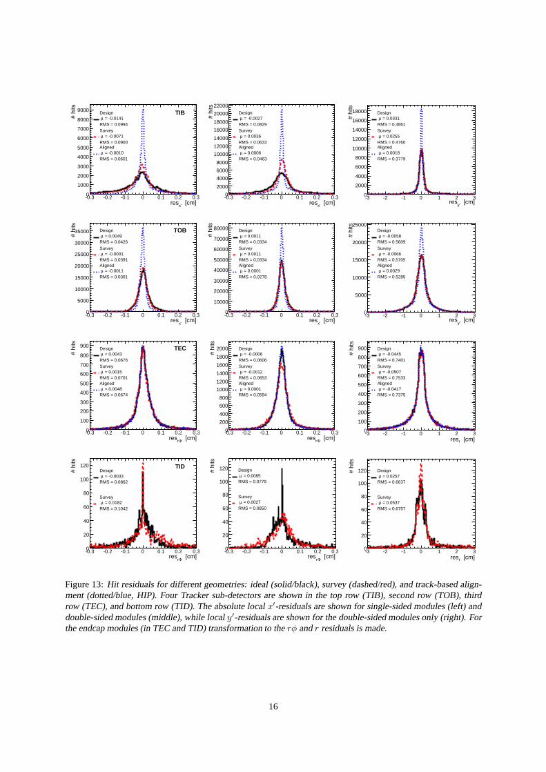
Improvements of the absolute track fitχ2 are observed when design geometry, survey measurements, and track-based alignment results are compared, as shown in Fig. 12. The averageχ2 changes from78 → 64 → 43 betweenthe three geometries, respectively. This is also visible inthe absolute hit residuals shown in Fig. 13. In general,an improvement can be observed by comparing the survey information to the design geometry, and comparing thetrack-based alignment to survey results. The residual meanvalues are closer to zero, and the standard deviationsare smaller.

In Fig. 14, the differences of the module positions between the design geometry and the geometry aligned withthe HIP algorithm are shown for TIB and TOB. There is a clear coherent movement of the four layers of the TIBin both radial (r) and azimuthal (φ) directions. The scale of the effect is rather large,1 − 2 mm. At the sametime, mounting placement uncertainty of modules in TOB is much smaller for both layers within the TOB andfor modules within layers. No obvious systematic deviations are observed apart from statistical scatter due tomounting precision.

Given good assembly precision of the TOB discussed above, the ideal geometry is a sufficiently good startinggeometry for TOB. Therefore, only high-level structure survey is considered for TOB and no detailed comparisoncan be discussed. As a result, TOB residuals in Fig. 13 do not change much between survey and ideal geometries,the two differing only in the overall TOB global position as shown in Fig. 4.

However, the situation is different for TIB and optical survey is necessary to improve the initial understanding ofthe module positions in this detector. From Figs. 4 and 14 it is evident that survey of the layer positions in TIBdoes not reflect the situation in data (displacement appearsto be even in the opposite direction). Therefore, we donot consider layer-level survey of TIB in our further analysis and do not include it in the track-based validation.However, the position of modules within a layer is reflected well in the optical survey. This is evident by significantimprovement of the TIB residuals between the ideal and survey geometries shown in Fig. 13, and in the trackχ2

in Fig. 12.

15

[cm]x’res-0.3 -0.2 -0.1 0 0.1 0.2 0.3

# hi

ts

0

1000

2000

3000

4000

5000

6000

7000

8000

9000

RMS = 0.0994 = -0.0141µ

Design

RMS = 0.0900 = -0.0071µ

Survey

RMS = 0.0601 = -0.0010µ

Aligned

TIB

[cm]x’res-0.3 -0.2 -0.1 0 0.1 0.2 0.3

# hi

ts

0

2000

4000

6000

8000

10000

12000

14000

16000

18000

20000

22000

RMS = 0.0829 = -0.0027µ

Design

RMS = 0.0633 = 0.0036µ

Survey

RMS = 0.0463 = 0.0006µ

Aligned

[cm]y’res-3 -2 -1 0 1 2 3

# hi

ts

0

2000

4000

6000

8000

10000

12000

14000

16000

18000

RMS = 0.4861 = 0.0331µ

Design

RMS = 0.4760 = 0.0255µ

Survey

RMS = 0.3779 = 0.0018µ

Aligned

[cm]x’

res-0.3 -0.2 -0.1 0 0.1 0.2 0.3

# hi

ts

0

5000

10000

15000

20000

25000

30000

35000

RMS = 0.0426 = 0.0049µ

Design

RMS = 0.0391 = -0.0001µ

Survey

RMS = 0.0301 = -0.0011µ

Aligned

TOB

[cm]x’

res-0.3 -0.2 -0.1 0 0.1 0.2 0.3

# hi

ts

0

10000

20000

30000

40000

50000

60000

70000

80000

RMS = 0.0334 = 0.0011µ

Design

RMS = 0.0334 = 0.0011µ

Survey

RMS = 0.0278 = 0.0001µ

Aligned

[cm]y’

res-3 -2 -1 0 1 2 3

# hi

ts

0

5000

10000

15000

20000

25000

RMS = 0.5609 = -0.0058µ

Design

RMS = 0.5705 = -0.0066µ

Survey

RMS = 0.5285 = 0.0029µ

Aligned

[cm]Φrres-0.3 -0.2 -0.1 0 0.1 0.2 0.3

# hi

ts

0

100

200

300

400

500

600

700

800

900

RMS = 0.0676 = 0.0043µ

Design

RMS = 0.0701 = 0.0015µ

Survey

RMS = 0.0674 = 0.0048µ

Aligned

TEC

[cm]Φrres-0.3 -0.2 -0.1 0 0.1 0.2 0.3

# hi

ts

0

200

400

600

800

1000

1200

1400

1600

1800

2000

RMS = 0.0606 = -0.0006µ

Design

RMS = 0.0653 = -0.0012µ

Survey

RMS = 0.0594 = 0.0001µ

Aligned

[cm]rres-3 -2 -1 0 1 2 3

# hi

ts

0

100

200

300

400

500

600

700

800

900

RMS = 0.7401 = -0.0445µ

Design

RMS = 0.7533 = -0.0507µ

Survey

RMS = 0.7375 = -0.0417µ

Aligned

[cm]Φrres-0.3 -0.2 -0.1 0 0.1 0.2 0.3

# hi

ts

0

20

40

60

80

100

120

RMS = 0.0862 = -0.0033µ

Design

RMS = 0.1042 = 0.0182µ

Survey

TID

[cm]Φrres

-0.3 -0.2 -0.1 0 0.1 0.2 0.3

# hi

ts

0

20

40

60

80

100

120

RMS = 0.0779 = 0.0085µ

Design

RMS = 0.0850 = 0.0027µ

Survey

[cm]rres-3 -2 -1 0 1 2 3

# hi

ts

0

20

40

60

80

100

120

RMS = 0.6637 = 0.0257µ

Design

RMS = 0.6757 = 0.0537µ

Survey

Figure 13:Hit residuals for different geometries: ideal (solid/black), survey (dashed/red), and track-based align-ment (dotted/blue, HIP). Four Tracker sub-detectors are shown in the top row (TIB), second row (TOB), thirdrow (TEC), and bottom row (TID). The absolute localx′-residuals are shown for single-sided modules (left) anddouble-sided modules (middle), while localy′-residuals are shown for the double-sided modules only (right). Forthe endcap modules (in TEC and TID) transformation to therφ andr residuals is made.

16

r [cm]20 30 40 50 60 70 80 90 100 110

r [c

m]

∆

-0.3

-0.25

-0.2

-0.15

-0.1

-0.05

-0

0.05

0.1

0.15

0.2

r [cm]20 30 40 50 60 70 80 90 100 110

z [c

m]

∆

-0.2

-0.15

-0.1

-0.05

-0

0.05

0.1

0.15

0.2

r [cm]20 30 40 50 60 70 80 90 100 110

[cm

]φ

∆ r

*

-0.3

-0.2

-0.1

0

0.1

0.2

0.3

Figure 14:Difference of the module positions between the measured (inHIP track-based alignment) and designgeometries for TIB (radiusr < 55 cm) and TOB (r > 55 cm). Projection on ther (left), z (middle), andφ (right)directions are shown. Only double-sided modules are considered in thez comparison.

4.3 Validation of the Track-Based Alignment

The three track-based alignment algorithms used in this study employ somewhat different statistical methods tominimise hit residuals and overall trackχ2. Therefore, comparison of their results is an important validation of thesystematic consistency of the methods.

To exclude the possibility of bad convergence of the track-based alignment, the alignment constants have beencomputed with random starting values. As an example, the starting values for the local shifts were drawn from aGaussian distribution with a variance ofσ = 200 µm. The corresponding results for the Kalman algorithm can beseen in Fig. 15, where in the upper two plots the computed global shifts for the sensitive coordinates are comparedto ones from the standard approach. Also, starting from the survey geometry rather than the ideal geometry wasattempted, as shown in the lower two plots. The results are compatible within their uncertainties as they arecalculated inside the Kalman algorithm.

The three alignment algorithms show similar distributionsof the trackχ2 shown in Fig. 16. HIP constants givethe smallest mean value whereas Kalman and Millepede have more tracks at lowχ2 values than the HIP constants.The three algorithms also have consistent residuals in all Tracker sub-detectors as shown in Fig. 17, though themost relevant comparison is in the barrel region (TIB and TOB) since the endcaps were not aligned at the modulelevel. For both Figs. 16 and 17, only modules selected for alignment have been taken into account in the refit andin the residual distributions.

A more quantitative view of the residual distributions and their improvement with alignment can be gained by look-ing at their widths. To avoid influence of modules not selected for alignment in the following, these are excludedfrom the residual distributions and from the track refits. Furthermore, taking the pure RMS of the distributionsgives a high weight to outliers e.g. from wrong hit assignments in data or artificially large misaligned modules insimulations (see Sec. 4.5). For this reason truncated mean and RMS values are calculated from the central 99.87%interval of each distribution, corresponding to 2.5σ for a Gaussian-distributed variable. The resulting widthsof theresidual distributions inx′ after alignment (HIP constants) are shown in Fig. 18 for the ten barrel layers. They areabout 120µm in TOB layers 2-5, between 200 and 300µm in TIB layers 2-3 and much larger in TIB layer 1 andTOB layer 6. This is due to the much larger track pointing uncertainty if the track prediction is an extrapolation tothe first and last hit of a track compared to interpolations for the hits in between, as can be seen from the secondcurve in Fig. 18. Here residuals from the first and last hits ofthe tracks are not considered. Residual widths in TIBdecrease clearly to about 150µm, making it evident that many tracks end within the TIB. TIB layer 1 and TOBlayer 6 now show especially small values since all remainingresiduals come from sensor overlap and have shorttrack interpolation distances.

The truncated mean and RMS values of these residual distributions are shown in Fig. 19 for the HIP alignmentresult compared to the results before alignment, showing clearly the improvements. The mean values are now closeto zero and the RMS decreases by at least almost a factor of two.

17

[cm]0x∆-0.2 -0.1 0 0.1 0.2

[cm

]r

x∆

-0.2

-0.1

0

0.1

0.2

[cm]0z∆-0.2 0 0.2

[cm

]r

z∆

-0.2

0

0.2

[cm]0x∆-0.2 -0.1 0 0.1 0.2

[cm

]s

x∆

-0.2

-0.1

0

0.1

0.2

[cm]0z∆-0.2 0 0.2

[cm

]s

z∆

-0.2

0

0.2

Figure 15: Comparison of the global shifts computed with different starting values, using the Kalman alignmentalgorithm. For the computation of∆x0 and∆z0 the starting values for parameters were set to 0, for∆xr and∆zr they were drawn from a Gaussian distribution and for∆XS and∆ZS they are taken from the module surveygeometry.

2χ0 100 200 300 400 500 600 700 800

# tr

acks

1

10

210

310

410

2χ0 20 40 60 80 100

# tr

acks

0

2000

4000

6000

8000

10000

12000

HIP: mean= 31.0

Millepede: mean= 46.1

Kalman: mean= 35.3

Figure 16:Distributions of the absoluteχ2-values of the track fits for the geometries resulting from HIP, Kalman,and Millepede alignment. The track fit is restricted to modules aligned by all three algorithms.

18

[cm]x’

res-0.3 -0.2 -0.1 0 0.1 0.2 0.3

# hi

ts

0

1000

2000

3000

4000

5000

6000RMS = 0.0498

= -0.0029µ HIP

RMS = 0.0639 = 0.0029µ

Millepede

RMS = 0.0461 = -0.0033µ

Kalman

TIB

[cm]x’

res-0.3 -0.2 -0.1 0 0.1 0.2 0.3

# hi

ts

0

2000

4000

6000

8000

10000

12000

14000

16000

18000

20000

22000

RMS = 0.0367 = 0.0003µ

HIP

RMS = 0.0408 = -0.0006µ

Millepede

RMS = 0.0314 = 0.0013µ

Kalman

[cm]y’

res-3 -2 -1 0 1 2 3

# hi

ts

0

2000

4000

6000

8000

10000RMS = 0.4655

= 0.0089µ HIP

RMS = 0.4769 = -0.0024µ

Millepede

RMS = 0.4686 = -0.0140µ

Kalman

[cm]x’

res-0.3 -0.2 -0.1 0 0.1 0.2 0.3

# hi

ts

0

5000

10000

15000

20000

25000

RMS = 0.0273 = -0.0009µ

HIP

RMS = 0.0284 = 0.0002µ

Millepede

RMS = 0.0266 = -0.0005µ

Kalman

TOB

[cm]x’

res-0.3 -0.2 -0.1 0 0.1 0.2 0.3

# hi

ts

0

10000

20000

30000

40000

50000RMS = 0.0288

= 0.0002µ HIP

RMS = 0.0279 = 0.0002µ

Millepede

RMS = 0.0278 = -0.0000µ

Kalman

[cm]y’

res-3 -2 -1 0 1 2 3

# hi

ts

0

2000

4000

6000

8000

10000

12000

14000

RMS = 0.4539 = -0.0049µ

HIP

RMS = 0.5118 = -0.0076µ

Millepede

RMS = 0.4581 = -0.0060µ

Kalman

[cm]Φrres-0.3 -0.2 -0.1 0 0.1 0.2 0.3

# hi

ts

0

100

200

300

400

500

600

RMS = 0.0711 = 0.0061µ

HIP

RMS = 0.0719 = 0.0057µ

Millepede

RMS = 0.0723 = 0.0050µ

Kalman

TEC

[cm]Φrres-0.3 -0.2 -0.1 0 0.1 0.2 0.3

# hi

ts

0

200

400

600

800

1000

RMS = 0.0648 = 0.0016µ

HIP

RMS = 0.0661 = 0.0005µ

Millepede

RMS = 0.0676 = 0.0008µ

Kalman

[cm]rres-3 -2 -1 0 1 2 3

# hi

ts

0

100

200

300

400

500

600

700

RMS = 0.6862 = -0.0332µ

HIP

RMS = 0.6963 = -0.0410µ

Millepede

RMS = 0.6937 = -0.0408µ

Kalman

Figure 17:Hit residuals for different geometries from three track-based algorithms: HIP (solid/black), Millepede(dashed/red), and Kalman (dotted/blue) based alignment. Three Tracker sub-detectors are shown in the top row(TIB), second row (TOB), and bottom row (TEC). The absolute local x′-residuals are shown for single-sidedmodules (left) and double-sided modules (middle), while localy′-residuals are shown for the double-sided modulesonly (right). For the endcap modules (TEC) transformation to therφ andr residuals is made. The track fit isrestricted to modules aligned by all three algorithms.

19

Layer 2 4 6 8 10

m)

µR

MS

(

0

100

200

300

400

500

600HIP alignment - all hits

HIP alignment - no first/last

Figure 18:Hit residual RMS in localx′ coordinate in ten layers of the barrel tracker, i.e. four layers of TIB and sixlayers of TOB, after track-based alignment with HIP. In contrast to the red circles, the blue squares are obtainedincluding residuals from the first and last hits of the track.Hits on modules not aligned are not considered in thetrack fit.

Layer 2 4 6 8 10

m)

µM

ean

(

-300

-200

-100

0

100

200

300 Data - no alignment

Data - HIP alignment

MC - design geometry

MC - tuned misalignment

m)µm, TOB = 50 µ(TIB = 80

Layer 2 4 6 8 10

m)

µR

MS

(

0

100

200

300

400

500

600 Data - no alignment

Data - HIP alignment

MC - ideal geometry

MC - tuned misalignment

m)µm, TOB = 50 µ(TIB = 80

Figure 19:Hit residual means in localx′ coordinate (left) and RMS (right) in ten layers of the barreltracker, i.e.four layers of TIB and six layers of TOB, shown in data before track-based alignment (red full circles), after track-based alignment (HIP, red full squares), in simulation withideal geometry (blue open circles) and in simulationafter tuning of misalignment according to data (blue open squares).

20

r [cm]20 30 40 50 60 70 80 90 100 110

r [c

m]

∆

-0.5

-0.4

-0.3

-0.2

-0.1

0

0.1

0.2

r [cm]20 30 40 50 60 70 80 90 100 110

z [c

m]

∆

-0.3

-0.2

-0.1

-0

0.1

0.2

0.3

0.4

r [cm]20 30 40 50 60 70 80 90 100 110

[cm

]φ

∆ r

*

-0.5

-0.4

-0.3

-0.2

-0.1

0

0.1

0.2

0.3

r [cm]20 30 40 50 60 70 80 90 100 110

r [c

m]

∆

-0.5

-0.4

-0.3

-0.2

-0.1

0

0.1

0.2

0.3

0.4

r [cm]20 30 40 50 60 70 80 90 100 110

z [c

m]

∆

-0.2

-0.1

0

0.1

0.2

0.3

0.4

0.5

r [cm]20 30 40 50 60 70 80 90 100 110

[cm

]φ

∆ r

*

-0.4

-0.3

-0.2

-0.1

-0

0.1

0.2

0.3

Figure 20:Difference of the module positions between the measured (intrack-based alignment) and design geome-tries shown for Kalman (top) and Millepede (bottom) algorithms for TIB (radiusr < 55 cm) and TOB (r > 55cm). Projection on ther (left), z (middle), andφ (right) directions are shown. Only double-sided modules areconsidered in thez comparison.

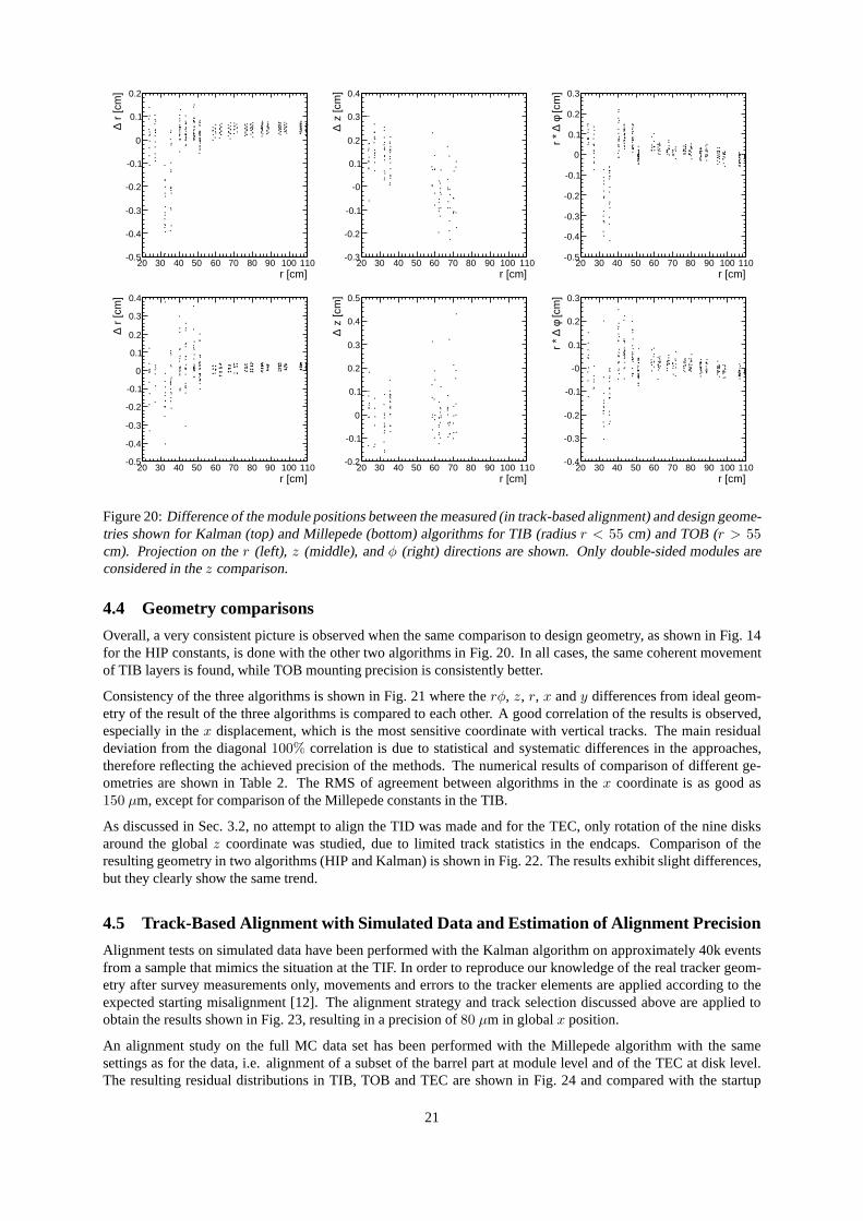
4.4 Geometry comparisons

Overall, a very consistent picture is observed when the samecomparison to design geometry, as shown in Fig. 14for the HIP constants, is done with the other two algorithms in Fig. 20. In all cases, the same coherent movementof TIB layers is found, while TOB mounting precision is consistently better.

Consistency of the three algorithms is shown in Fig. 21 wheretherφ, z, r, x andy differences from ideal geom-etry of the result of the three algorithms is compared to eachother. A good correlation of the results is observed,especially in thex displacement, which is the most sensitive coordinate with vertical tracks. The main residualdeviation from the diagonal100% correlation is due to statistical and systematic differences in the approaches,therefore reflecting the achieved precision of the methods.The numerical results of comparison of different ge-ometries are shown in Table 2. The RMS of agreement between algorithms in thex coordinate is as good as150 µm, except for comparison of the Millepede constants in the TIB.

As discussed in Sec. 3.2, no attempt to align the TID was made and for the TEC, only rotation of the nine disksaround the globalz coordinate was studied, due to limited track statistics in the endcaps. Comparison of theresulting geometry in two algorithms (HIP and Kalman) is shown in Fig. 22. The results exhibit slight differences,but they clearly show the same trend.

4.5 Track-Based Alignment with Simulated Data and Estimation of Alignment Precision

Alignment tests on simulated data have been performed with the Kalman algorithm on approximately 40k eventsfrom a sample that mimics the situation at the TIF. In order toreproduce our knowledge of the real tracker geom-etry after survey measurements only, movements and errors to the tracker elements are applied according to theexpected starting misalignment [12]. The alignment strategy and track selection discussed above are applied toobtain the results shown in Fig. 23, resulting in a precisionof 80 µm in globalx position.

An alignment study on the full MC data set has been performed with the Millepede algorithm with the samesettings as for the data, i.e. alignment of a subset of the barrel part at module level and of the TEC at disk level.The resulting residual distributions in TIB, TOB and TEC areshown in Fig. 24 and compared with the startup

21

[cm] (HIP)φ ∆ r -0.3 -0.2 -0.1 0 0.1 0.2 0.3

[cm

] (M

P)

φ ∆

r

-0.3

-0.2

-0.1

0

0.1

0.2

0.3 = 0.790 ρ

[cm] (HIP)φ ∆ r -0.3 -0.2 -0.1 0 0.1 0.2 0.3

[cm

] (K

AA

)φ

∆ r

-0.3

-0.2

-0.1

0

0.1

0.2

0.3 = 0.910 ρ

[cm] (MP)φ ∆ r -0.3 -0.2 -0.1 0 0.1 0.2 0.3

[cm

] (K

AA

)φ

∆ r

-0.3

-0.2

-0.1

0

0.1

0.2

0.3 = 0.855 ρ

r [cm] (HIP)∆ -0.3 -0.2 -0.1 0 0.1 0.2 0.3

r [c

m] (

MP

)∆

-0.3

-0.2

-0.1

0

0.1

0.2

0.3 = 0.679 ρ

r [cm] (HIP)∆ -0.3 -0.2 -0.1 0 0.1 0.2 0.3

r [c

m] (

KA

A)

∆

-0.3

-0.2

-0.1

0

0.1

0.2

0.3 = 0.669 ρ

r [cm] (MP)∆ -0.3 -0.2 -0.1 0 0.1 0.2 0.3

r [c

m] (

KA

A)

∆

-0.3

-0.2

-0.1

0

0.1

0.2

0.3 = 0.487 ρ

z [cm] (HIP)∆ -0.4 -0.3 -0.2 -0.1 -0 0.1 0.2 0.3 0.4

z [c

m] (

MP

)∆

-0.4

-0.3

-0.2

-0.1

-0

0.1

0.2

0.3

0.4 = 0.715 ρ

z [cm] (HIP)∆ -0.4 -0.3 -0.2 -0.1 -0 0.1 0.2 0.3 0.4

z [c

m] (

KA

A)

∆

-0.4

-0.3

-0.2

-0.1

-0

0.1

0.2

0.3

0.4 = 0.682 ρ

z [cm] (MP)∆ -0.4 -0.3 -0.2 -0.1 -0 0.1 0.2 0.3 0.4

z [c

m] (

KA

A)

∆

-0.4

-0.3

-0.2

-0.1

-0

0.1

0.2

0.3

0.4 = 0.529 ρ

x [cm] (HIP)∆ -0.4 -0.3 -0.2 -0.1 -0 0.1 0.2 0.3 0.4

x [c

m] (

MP

)∆

-0.4

-0.3

-0.2

-0.1

-0

0.1

0.2

0.3

0.4 = 0.821 ρ

x [cm] (HIP)∆ -0.4 -0.3 -0.2 -0.1 -0 0.1 0.2 0.3 0.4

x [c

m] (

KA

A)

∆

-0.4

-0.3

-0.2

-0.1

-0

0.1

0.2

0.3

0.4 = 0.911 ρ

x [cm] (MP)∆ -0.4 -0.3 -0.2 -0.1 -0 0.1 0.2 0.3 0.4

x [c

m] (

KA

A)

∆

-0.4

-0.3

-0.2

-0.1

-0

0.1

0.2

0.3

0.4 = 0.845 ρ

y [cm] (HIP)∆ -0.8 -0.6 -0.4 -0.2 -0 0.2 0.4 0.6 0.8

y [c

m] (

MP

)∆

-0.8

-0.6

-0.4

-0.2

-0

0.2

0.4

0.6

0.8 = 0.658 ρ

y [cm] (HIP)∆ -0.8 -0.6 -0.4 -0.2 -0 0.2 0.4 0.6 0.8

y [c

m] (

KA

A)

∆

-0.8

-0.6

-0.4

-0.2

-0

0.2

0.4

0.6

0.8 = 0.836 ρ

y [cm] (MP)∆ -0.8 -0.6 -0.4 -0.2 -0 0.2 0.4 0.6 0.8

y [c

m] (

KA

A)

∆

-0.8

-0.6

-0.4

-0.2

-0

0.2

0.4

0.6

0.8 = 0.672 ρ

Figure 21: Direct comparison of differences from ideal geometry inrφ (top), z (second row),r (third row),x (fourth row), andy (bottom) between Millepede and HIP (left), Kalman and HIP (middle), and Kalman andMillepede (right). The correlation coefficientρ is stated.

22

z [mm]1400 1600 1800 2000 2200 2400 2600 2800

[mra

d]φ∆

-1

-0.5

0

0.5

1 Algorithm

HIP

Kalman

Figure 22:Rotations of the TEC disks around the globalz in comparison of the measured (in track-based align-ment) and design geometries for TEC. Two track-based results are shown: HIP (triangles) and Kalman filter(circles) algorithms.

Mean -0.002515

RMS 0.008347

x [cm]∆-0.05 0 0.050

5

10

15

20

25

30Mean -0.002515

RMS 0.008347

Mean 0.01003

RMS 0.03205

y [cm]∆-0.15 -0.1 -0.05 0 0.05 0.1 0.150

2

4

6

8

10

12Mean 0.01003

RMS 0.03205

Mean 0.002994

RMS 0.05544

z [cm]∆-0.15 -0.1 -0.05 0 0.05 0.1 0.150

2

4

6

8

10

12

14

16

Mean 0.002994

RMS 0.05544

Figure 23: Alignment resolution in global coordinates achieved with the Kalman alignment algorithm on simulateddata.

23

Table 2: Comparison of the globalx, y andz RMS difference (inµm) of module positions between differentgeometries indicated in the first two columns for TOB and TIB.Single-sided (SS) and double-sided (DS) modulesare shown together and separately.

Geom 1 Geom 2 difference TIB TIB (SS) TIB (DS) TOB TOB (SS) TOB (DS)HIP Design ∆z - - 638 - - 806MP Design ∆z - - 787 - - 1139

KAA Design ∆z - - 706 - - 1053KAA HIP ∆z - - 429 - - 487MP HIP ∆z - - 533 - - 805

KAA MP ∆z - - 698 - - 614HIP Design ∆x 526 438 581 130 108 142MP Design ∆x 623 500 653 236 206 208

KAA Design ∆x 543 500 519 237 215 173KAA HIP ∆x 165 138 193 159 156 74MP HIP ∆x 341 297 383 162 148 151

KAA MP ∆x 304 226 396 123 132 97HIP Design ∆y 1353 914 1639 93 88 103MP Design ∆y 1527 1173 1488 144 125 183

KAA Design ∆y 1751 541 2180 141 132 164KAA HIP ∆y 850 471 1036 94 80 123MP HIP ∆y 1202 1043 1417 101 80 139

KAA MP ∆y 1324 842 1845 59 57 63

misalignment [12] and the ideal geometry. Comparison with the distributions obtained from data using the designgeometry (Fig. 17) reveals that in TIB and TOB the starting misalignment is overestimated while in TEC it isslightly underestimated. The residual widths after alignment are generally much smaller than those obtained fromthe aligned data, especially in the TIB. This could be due to the larger statistics of the simulation data sample, butalso due to effects not properly simulated, e.g. relative misalignment of the two components of a double-sidedmodule or possible differences in the momentum spectrum of Monte Carlo.

The results of the truncated RMS of the layerwise residual distributions in Fig. 19 are used to estimate alignmentprecision in the aligned barrel region via comparison with simulations. Different misalignment scenarios havebeen applied to the ideal (“true”) Tracker geometry used in reconstructing the simulated data until truncated RMSvalues are found to be similar to the ones in data in all layers. The modules in TIB and TOB have been randomlyshifted in three dimensions by Gaussian distributions. Theinfluence of possibly large misalignments from the tailsof these Gaussians is reduced by truncating the distributions as stated above.

Besides the truncated mean and RMS values from data before and after alignment, Fig. 19 shows also the resultsfrom the simulation reconstructed with the ideal geometry and reconstructed with a random misalignment accord-ing to Gaussian distributions with standard deviations of 50µm and 80µm in the TOB and the TIB, respectively. Itcan be clearly seen that the simulation with the ideal, i.e. true, geometry has smaller widths than the data, especiallyin the TIB. On the other hand, the geometry with a simulated misalignment of 50µm and 80µm, respectively,resembles rather well the data after alignment, such that these numbers can well be taken as an estimate of the sizeof the remaining misalignment.

5 Stability of the Tracker Geometry with Temperature and Time5.1 Stability of the Tracker Barrels

In order to investigate stability of the tracker componentswith respect to the cooling temperature and stress due toTEC insertion, full alignment of the Tracker in different periods has been performed and the positions of modulesin space are compared. The advantage of this approach is thatwe can see module movements directly, but thepotential problem is that we may be misled by a systematic effect or a weakly constrained misalignment. Statisticalscatter of up to 100µm limits the resolution of the method. These tests have been done with the HIP algorithm.

1. +15◦C (A1, before TEC- insertion) vs. +10◦C (C10, after TEC- insertion).

24

[cm]x’

res-0.3 -0.2 -0.1 0 0.1 0.2 0.3

# hi

ts

0

5000

10000

15000

20000

25000RMS = 0.0310

= -0.0003µ Ideal MC

RMS = 0.1265 = 0.0151µ

Misaligned MC

RMS = 0.0343 = 0.0011µ

Aligned MC

TIB

[cm]x’

res-0.3 -0.2 -0.1 0 0.1 0.2 0.3

# hi

ts

0

10000

20000

30000

40000

50000

60000

RMS = 0.0238 = 0.0001µ

Ideal MC

RMS = 0.1177 = 0.0131µ

Misaligned MC

RMS = 0.0288 = 0.0003µ

Aligned MC

[cm]y’

res-3 -2 -1 0 1 2 3

# hi

ts

0

5000

10000

15000

20000

25000

30000

RMS = 0.3826 = -0.0048µ

Ideal MC

RMS = 0.4617 = 0.0432µ

Misaligned MC

RMS = 0.3811 = -0.0005µ

Aligned MC

[cm]x’

res-0.3 -0.2 -0.1 0 0.1 0.2 0.3

# hi

ts

0

10000

20000

30000

40000

50000

RMS = 0.0300 = -0.0010µ

Ideal MC

RMS = 0.0597 = -0.0138µ

Misaligned MC

RMS = 0.0311 = -0.0018µ

Aligned MC

TOB

[cm]x’

res-0.3 -0.2 -0.1 0 0.1 0.2 0.3

# hi

ts

0

20

40

60

80

100

310×

RMS = 0.0250 = -0.0003µ

Ideal MC

RMS = 0.0339 = -0.0048µ

Misaligned MC

RMS = 0.0252 = -0.0008µ

Aligned MC

[cm]y’

res-3 -2 -1 0 1 2 3

# hi

ts

0

5000

10000

15000

20000

25000

30000

RMS = 0.4320 = -0.0032µ

Ideal MC

RMS = 0.5305 = -0.0071µ

Misaligned MC

RMS = 0.4445 = -0.0039µ

Aligned MC

[cm]Φrres-0.3 -0.2 -0.1 0 0.1 0.2 0.3

# hi

ts

0

500

1000

1500

2000

2500

3000

3500

4000

4500

RMS = 0.0451 = 0.0011µ

Ideal MC

RMS = 0.0514 = 0.0022µ

Misaligned MC

RMS = 0.0520 = 0.0025µ

Aligned MC

TEC

[cm]Φrres-0.3 -0.2 -0.1 0 0.1 0.2 0.3

# hi

ts

0

1000

2000

3000

4000

5000

6000

7000

8000

RMS = 0.0376 = 0.0003µ

Ideal MC

RMS = 0.0405 = 0.0001µ

Misaligned MC

RMS = 0.0405 = -0.0005µ

Aligned MC

[cm]rres-3 -2 -1 0 1 2 3

# hi

ts

0

500

1000

1500

2000

2500

3000

3500

4000

RMS = 0.5049 = 0.0026µ

Ideal MC

RMS = 0.5285 = 0.0019µ

Misaligned MC

RMS = 0.5270 = 0.0066µ

Aligned MC

Figure 24:Hit residuals for different geometries in different conditions for the simulated data sample: ideal geom-etry (solid/black), misaligned geometry according to expected starting misalignment (dashed/red), and geometryafter alignment (dotted/blue). Three Tracker sub-detectors are shown in the top row (TIB), second row (TOB),and bottom row (TEC). The absolute localx-residuals are shown for single-sided modules (left) and double-sidedmodules (middle), while localy-residuals are shown for the double-sided modules only (right). For the endcapmodules (TEC) transformation to therφ andr residuals is made.

25

r [cm]20 30 40 50 60 70 80 90 100 110

x [c

m]

∆

-0.03

-0.02

-0.01

0

0.01

0.02

0.03

r [cm]20 30 40 50 60 70 80 90 100 110

y [c

m]

∆

-0.15

-0.1

-0.05

0

0.05

0.1

r [cm]20 30 40 50 60 70 80 90 100 110

z [c

m]

∆

-0.14

-0.12

-0.1

-0.08

-0.06

-0.04

-0.02

0

0.02

0.04

0.06

Mean 0.001396

RMS 0.007528

x [cm]∆-0.03 -0.02 -0.01 0 0.01 0.02 0.03

#mod

ules

0

5

10

15

20

25

30Mean 0.001396

RMS 0.007528TIB

Mean -0.005325

RMS 0.04042

y [cm]∆-0.15 -0.1 -0.05 0 0.05 0.1

#mod

ules

0

2

4

6

8

10

12

14

Mean -0.005325

RMS 0.04042

Mean -0.00642

RMS 0.02617

z [cm]∆-0.1 -0.05 0 0.05 0.1

#mod

ules

0

1

2

3

4

5Mean -0.00642

RMS 0.02617

Mean -0.0003391

RMS 0.004431

x [cm]∆-0.03 -0.02 -0.01 0 0.01 0.02 0.03

#mod

ules

0

5

10

15

20

25

30

35

Mean -0.0003391

RMS 0.004431TOB

Mean 0.003641

RMS 0.002826

y [cm]∆-0.15 -0.1 -0.05 0 0.05 0.1

#mod

ules

0

10

20

30

40

50

60

70

80Mean 0.003641

RMS 0.002826

Mean -0.001143

RMS 0.02727

z [cm]∆-0.1 -0.05 0 0.05 0.1

#mod

ules

0

1

2

3

4

5

6

7

8Mean -0.001143

RMS 0.02727

Figure 25: Differences in determinedx- (left), y- (centre) andz-positions (right, only double-sided) of activemodules comparing the configurations before and after TEC- insertion. The differences are stated as a function ofthe module radiusr (top row) and for modules in TIB (middle row) and TOB (bottom row) separately.

This test is intended to show the effect of the insertion of a mechanical object between two data-takingconditions. Fig. 25 shows the shifts between the two sets of aligned positions in globalx, y andz as afunction of the radial coordinate and projected separatelyfor TIB and TOB.

In the TOB, a very small layer-wise shift is visible, especially in layers one and two.

As can be seen from Fig. 26, there is no further structure as a function of thez coordinate. This could bea hint of a small layer-wise rotation around thez axis. In the TIB, coherent movements are larger in theazimuthal direction and are also layer-dependent; but here, they are reflected in the corresponding structuresin the longitudinal direction: the movement is largest closer to z = 0 and is reduced to small values atlargez (see Fig. 26). We interpret it as a layer- and side-dependenttwist where the outer edges inz arebetter constrained due to the mechanical mounting technique. However, it is also possible that there is notenough information to constrain the “weak” degrees of freedom, or this could be an artificial effect dueto different modules being aligned in different configurations and different track samples due to differenttrigger configurations.

2. -10 ◦C (C−10, default sample) vs. +10◦C (C10).

This test is intended to show the effect of a large temperature gap between two data-taking conditions.Figure 27 shows the shifts between the two sets of aligned positions in globalx, y andz as a function of theradial coordinate and projected separately for TIB and TOB.

All deviations are within what appears to be statistical scatter, so this comparison does not show statisticallysignificant movements. In the TOB, though certain layers exhibit larger scatter than the others, there is noevidence of any coherent shift. In the TIB, there are hints ofa small systematic shift vs. the layer numberincreasing towards outer layers, that could be caused by a relative movement between the cylinders or arotation around the globalz axis. No dependence vs. globalz is observed, excluding large effects of a

26

z [cm]0 10 20 30 40 50 60

x [c

m]

∆

-0.03

-0.02

-0.01

0

0.01

0.02

0.03TIB

z [cm]0 10 20 30 40 50 60

z [c

m]

∆

-0.14

-0.12

-0.1

-0.08

-0.06

-0.04

-0.02

0

0.02

0.04

z [cm]10 20 30 40 50 60 70 80 90 100

x [c

m]

∆

-0.025

-0.02

-0.015

-0.01

-0.005

0

0.005

0.01

0.015

0.02 TOB

z [cm]10 20 30 40 50 60 70 80

z [c

m]

∆

-0.08

-0.06

-0.04

-0.02

0

0.02

0.04

0.06

Figure 26:Differences in determinedx- (left) andz-positions (right, only double-sided) of active modules com-paring the configurations before and after TEC- insertion asa function of the moduler-position for modules inTIB (upper row) and TOB (bottom row).

r [cm]20 30 40 50 60 70 80 90 100 110

x [c

m]

∆

-0.04

-0.03

-0.02

-0.01

0

0.01

0.02

0.03

r [cm]20 30 40 50 60 70 80 90 100 110

y [c

m]

∆

-0.1

-0.05

0

0.05

0.1

0.15

0.2

0.25

r [cm]20 30 40 50 60 70 80 90 100 110

z [c

m]

∆

-0.08

-0.06

-0.04

-0.02

0

0.02

0.04

0.06

0.08

0.1

0.12

Mean 2.8e-05

RMS 0.007999

x [cm]∆-0.03 -0.02 -0.01 0 0.01 0.02 0.03

#mod

ules

0

2

4

6

8

10

12

14

16

18

Mean 2.8e-05

RMS 0.007999

TIB

Mean 0.005567

RMS 0.04072

y [cm]∆-0.2 -0.15 -0.1 -0.05 -0 0.05 0.1 0.15 0.2

#mod

ules

0

5

10

15

20

25

30

35Mean 0.005567

RMS 0.04072

Mean 0.001333

RMS 0.03512

z [cm]∆-0.1 -0.05 0 0.05 0.1

#mod

ules

0

1

2

3

4

5

6

7

8Mean 0.001333

RMS 0.03512

Mean 0.0004975

RMS 0.002848

x [cm]∆-0.03 -0.02 -0.01 0 0.01 0.02 0.03

#mod

ules

0

5

10

15

20

25

30

35Mean 0.0004975

RMS 0.002848

TOB

Mean -0.006436

RMS 0.004038

y [cm]∆-0.2 -0.15 -0.1 -0.05 -0 0.05 0.1 0.15 0.2

#mod

ules

0

10

20

30

40

50

60

70

80

90Mean -0.006436

RMS 0.004038

Mean 0.001791

RMS 0.01911

z [cm]∆-0.1 -0.05 0 0.05 0.1

#mod

ules

0

1

2

3

4

5

6

7

8Mean 0.001791

RMS 0.01911

Figure 27: Differences in determinedx- (left), y- (centre) andz-positions (right, only double-sided) of activemodules comparing the +10◦C and -10◦C configurations. The differences are stated as a function ofthe moduleradiusr (top row) and for modules in TIB (middle row) and TOB (bottom row) separately.

27

rotation about they direction or a twist.

5.2 Stability of the Tracker Endcap

For the TEC stability validation, a comparison is made of thedisk alignment with tracks, using the Kalman filteralgorithm, for the temperature levels: room temperature, 10 ◦C, -1◦C, -10◦C, -15◦C, and 14◦C. The alignmentparameters calculated with these data sets are shown on the left of Fig. 28. The determined alignment parametersfor the different tracker temperatures agree with each other within their errors. Disk nine is never hit in the datataken at -15◦C or 14◦C; therefore, there are only eight alignment parameters available at these temperature levels.At -15 ◦C, the experiment setup changed: Only the back petals have been activated because there was not enoughcooling power.

z [mm]1400 1600 1800 2000 2200 2400 2600 2800

[mra

d]φ∆

-0.6

-0.4

-0.2

0

0.2

0.4

0.6Data set

C°T = 15 C°T = 10 C°T = -1 C°T = -10 C°T = -15

C°T = 14

z [mm]1400 1600 1800 2000 2200 2400 2600 2800

[mra

d]φ∆

-0.6

-0.4

-0.2

0

0.2

0.4

0.6 Data set

TIF (merged T)

Aachen

Figure 28:Alignment parameter∆φ for TEC disks at six tracker temperature levels (left). Alignment parameter∆φ for TEC disks, determined with TIF data and Aachen data usingan obsolete, but common geometry (right).

In addition, during the TEC integration in Aachen, tracks from cosmic muons have been recorded. Here, the TEChad been positioned vertically. For each sector, data had been taken separately after its integration. The processingof these data had been done using a now obsolete geometry description. The modules on TEC rings 2 and 5 aredisplaced in this geometry by up to 140µm.

To create equivalent results, an alignment in∆φ is determined with tracks from TIF data and compared with resultsfrom tracks of sector 2 and 3 of the data from Aachen. To avoid major differences in the alignment results due tochanges in the geometry, the tracks of the TIF data are reconstructed using the same geometry as used for Aachendata. The right of Fig. 28 shows the alignment parameters gained from TIF and Aachen data. Except for somechanges in disks 1, 3, and 4 of the order of 0.2 mrad, the TEC seems to have been stable during transportation fromAachen to Geneva, tilting from a vertical to a horizontal position, and integration into the tracker. Two petals havebeen replaced in the active TEC sectors before taking the TIFdata: A back petal of disk 3 and a front petal of disk4. Thus, changes in the corrections∆φ of these disks are expected.

6 Laser Alignment System Analysis and DiscussionIn this section, we discuss results from the Laser AlignmentSystem. Analysis of the measurements from thissystem have not been integrated with the track-based statistical methods. Therefore, we discuss the data analysisand results independently.

6.1 Data Taking

At the TIF, data was taken with the laser alignment system. Onthe z+ side of the tracker, the beams from thealignment tubes of sector 1, 2 and 3 were seen by the barrel modules. The endcap sectors 2 and 3 were operatedwith the TEC internal beams and the alignment tubes of those sectors. Data was taken before cooling the trackerdown, during the cooling cycle, and at the end, when the tracker was back at room temperature.

As we mentioned earlier, the Laser Alignment System was designed to measure deformations and movements ofthe tracker support structures. To do this properly, the whole φ-range of the laser beams needs to be operated.The fact that only a slice of the tracker was operated during the TIF tests means that no complete picture of thetracker alignment parameters could be obtained. Nevertheless, the data taking was very useful to verify the proper

28

functioning of the laser beams and the laser data taking. First of all, the evolution of the measured laser spotpositions with temperature was studied. Movements could beeither due to thermal deformations of the trackerstructure, or caused by small movements of the beamsplitterholders. Then, the data taken in the TEC sectors canbe compared to the data obtained during the TEC integration.Here, observed differences could also have beencaused by the handling, transport and insertion of the endcaps.

6.2 Results from Alignment Tubes

The alignment tubes were first operated at room temperature.Then, as the tracker was gradually cooled down, theywere measured at 10◦C, -1 ◦C, -15◦C and finally again at room temperature, after the tracker hadbeen warmedup again. The measured laser spot positions were all compared to the first measurements at room temperature.The result is shown in Fig. 29. The largest changes of about 600 µm were observed in the TOB. The observedmovements could come either from movements of the tracker structure, or from movements of the laser beams.Nevertheless, two bounds can be given. First, one could assume that all detected movements were due to trackerstructure deformations. In this case, we would have observed movements of 600µm. On the other hand, one couldtry to absorb as much as of the observed laser spot changes into movements of the laser beams. In this case, onecalculates the tilt of the laser beams and rotations of the alignment tubes that fit best to the observed laser spotmovements. After subtracting this contribution, the remaining laser spot movements would be due to the trackersupport deformation. This is shown in Fig. 30. Now the maximal movements of the tracker would be less than100µm.

6.3 Comparison of LAS and Track Based Alignment Results

A comparison is made between the Laser Alignment System residuals and the TEC disk alignment results usingtrack based alignment at different temperatures. Corrections are applied to the residuals because the beam splittersused by the LAS are known to emit two non-perfectly parallel laser beams. Considering the laser beamspotradii, the residuals measured at room temperature are transformed into disk rotations. The disc corrections,∆φ,estimated with the Kalman alignment algorithm from cosmic track data are used for comparison. There are nosignificant changes in the TEC alignment evaluated with track based alignment at different temperatures, so thetrack data merged from all temperature runs exceptT = −15 ◦C were used to obtain a better precision.

Because the exact direction of the laser beams is unknown, a linear dependence ofφ on z cannot be determinedusing the LAS residuals. Therefore, mean and slope (as a function of z) of the corrections to the disc rotations aresubtracted. The same is done with the results from the Kalmanalignment algorithm to use a common coordinatesystem. The remaining corrections are displayed in Fig. 31.For LAS, the mean and RMS of the four measurementsestimated from the four active laser beams in the endcap are shown for each disk. There are differences among theLAS corrections for the same disk of up to 0.7 mrad. These differences are interpreted as misalignment on moduleand petal level. Considering the accuracy of the Kalman alignment parameters and the spread of the LAS results,the estimated corrections show a good agreement.

7 Summary and ConclusionWe have presented results of the CMS tracker alignment analysis at the Integration Facility at CERN by meansof cosmic tracks, optical survey information, and the LaserAlignment System. The first alignment of the activesilicon modules with three different statistical approaches was performed, using cosmic track events collected withthe partially active CMS tracker during spring and summer of2007.

Optical survey measurements of the tracker were validated with the track residuals in the active part of the de-tector. Clear improvement with respect to the design geometry description was seen. Overall, further significantimprovements in trackχ2 and track-hit residuals are achieved after track-based alignment of the tracker at TIF,when compared either to design or survey geometry.

Detailed studies have been performed on the Tracker Inner and Outer Barrel alignment with tracks. The typicalachieved precision on module position measurement in the local x coordinate is estimated to be about 50µmand 80µm in the Tracker Outer and Inner Barrels, respectively. However, since no magnetic field was appliedin the tracker, no momentum estimate of the cosmic tracks waspossible. Therefore, detailed understanding ofalignment precision suffers from uncertainties in multiple scattering of tracks with unknown momentum, thisbeing the dominant contribution to the hit resolution. For this reason, the above alignment precision estimates arebased on prediction from simulations of hit residuals and may overestimate the detector misalignment.

29

z [mm]200 400 600 800 1000 1200 1400 1600 1800

[mm

]φ∆ ×

r

-0.6-0.4-0.2

00.20.40.6

z [mm]200 400 600 800 1000 1200 1400 1600 1800

[mm

]φ∆ ×

r

-0.6-0.4-0.2

00.20.40.6 Sector 1

Sector 2Sector 3

C°10

z [mm]200 400 600 800 1000 1200 1400 1600 1800

[mm

]φ∆ ×

r

-0.6-0.4-0.2

00.20.40.6

z [mm]200 400 600 800 1000 1200 1400 1600 1800

[mm

]φ∆ ×

r

-0.6-0.4-0.2

00.20.40.6

C°-1

z [mm]200 400 600 800 1000 1200 1400 1600 1800

[mm

]φ∆ ×

r

-0.6-0.4-0.2

00.20.40.6

z [mm]200 400 600 800 1000 1200 1400 1600 1800

[mm

]φ∆ ×

r

-0.6-0.4-0.2

00.20.40.6

C°-10

z [mm]200 400 600 800 1000 1200 1400 1600 1800

[mm

]φ∆ ×

r

-0.6-0.4-0.2

00.20.40.6

z [mm]200 400 600 800 1000 1200 1400 1600 1800

[mm

]φ∆ ×

r

-0.6-0.4-0.2

00.20.40.6

C°-15

Figure 29: Changes in laser spot positions while cooling down the tracker.

30

z [mm]200 400 600 800 1000 1200 1400 1600 1800

[mm

]φ∆ ×

r

-0.6-0.4-0.2

00.20.40.6

z [mm]200 400 600 800 1000 1200 1400 1600 1800

[mm

]φ∆ ×

r

-0.6-0.4-0.2

00.20.40.6 Sector 1

Sector 2Sector 3

C°10

z [mm]200 400 600 800 1000 1200 1400 1600 1800

[mm

]φ∆ ×

r

-0.6-0.4-0.2

00.20.40.6

z [mm]200 400 600 800 1000 1200 1400 1600 1800

[mm

]φ∆ ×

r

-0.6-0.4-0.2

00.20.40.6

C°-1

z [mm]200 400 600 800 1000 1200 1400 1600 1800

[mm

]φ∆ ×

r

-0.6-0.4-0.2

00.20.40.6

z [mm]200 400 600 800 1000 1200 1400 1600 1800

[mm

]φ∆ ×

r

-0.6-0.4-0.2

00.20.40.6

C°-10

z [mm]200 400 600 800 1000 1200 1400 1600 1800

[mm

]φ∆ ×

r

-0.6-0.4-0.2

00.20.40.6

z [mm]200 400 600 800 1000 1200 1400 1600 1800

[mm

]φ∆ ×

r

-0.6-0.4-0.2

00.20.40.6 C°-15

Figure 30: Changes in laser spot positions while cooling down the tracker, removing the maximum contributionthat can be due to movements of the alignment tube.

31

z [mm]1400 1600 1800 2000 2200 2400 2600 2800

[mra

d]φ∆

-1

-0.5

0

0.5

1Data set

Cosmic tracks

LAS

Figure 31:Corrections∆φ for TEC disks determined with track based alignment and LAS residuals.

Consistent alignment results have been obtained with threedifferent alignment algorithms Direct comparison ofobtained geometries indicate∼150µm consistency in the precisely measured coordinate, consistent with the indi-rect interpretation of track residuals. However, certainχ2-invariant deformations appear in the alignment procedurewhen using only cosmic tracks. Theseχ2-invariant deformations do not affect track residuals and therefore are notvisible in the alignment minimisation, thus limiting understanding of relative position of all modules in space fromthe pure geometrical point of view.

Alignment of the Tracker Endcap was performed at the disk level, both with tracks and by operating the CMSLaser Alignment System and showed good agreement between the two results.

No significant deformations of the tracker have been observed under stress and with variation of temperature,within the resolution of the alignment methods.

The operation of the Laser Alignment System during the TIF slice test has shown that the laser beams operateproperly. Useful laser signals were detected by all modulesthat were illuminated by the laser beams. In theworst-case scenario, where all observed laser spot shifts are assumed to come from structure deformations, themovements would be up to 600µm. Assuming that most of the observed changes were coming from laser beamand alignment tube movements, shifts go down below 100µm. To disentangle the two contributions and geta complete picture of the tracker deformations, more beams,distributed around all the 2π φ-range, have to beoperated.

Finally, experience gained in alignment analysis of the silicon modules at the Tracker Integration Facility is valu-able in preparation for the full CMS tracker alignment, which is crucial for high precision necessary to achieve thedesign physics goals of the CMS detector.

8 AcknowledgmentsWe thank the administrative staff at CERN and other Tracker Institutes. This work has been supported by: theAustrian Federal Ministry of Science and Research; the Belgium Fonds de la Recherche Scientifique and Fondsvoor Wetenschappelijk Onderzoek; the Academy of Finland and Helsinki Institute of Physics; the Institut Nationalde Physique Nucleaire et de Physique des Particules / CNRS,France; the Bundesministerium fur Bildung undForschung, Germany; the Istituto Nazionale di Fisica Nucleare, Italy; the Swiss Funding Agencies; the Science andTechnology Facilities Council, UK; the US Department of Energy, and National Science Foundation. Individualshave received support from the Marie-Curie IEF program (European Union) and the A. P. Sloan Foundation.

———————————————————————–

32

References[1] The CMS Tracker System Project TDR, CERN/LHCC 98-6, CMS TDR 5 (1998).

The CMS Tracker System Project TDR Addendum, CERN/LHCC 2000-016, CMS TDR 5 Addendum 1(2000).

[2] CMS Collaboration, S. Chatrchyanet al., “The CMS Experiment at the CERN LHC”, 2008 JINST3 S08004.

[3] W. Adam et al., “Track Reconstruction with Cosmic Ray Data at the Tracker Integration Facility”, CMSNOTE in preparation.

[4] W. Adamet al., “Silicon Strip Tracker Detector Performance with Cosmic Ray Data at the Tracker IntegrationFacility”, CMS NOTE 2008/032.

[5] P. Biallass, T. Hebbeker, “Improved Parameterization of the Cosmic Muon Flux for the Generator CMSC-GEN”, CMS NOTE 2007/033.

[6] M. Boezioet al., “Energy spectra of atmospheric muons measured with the CAPRICE98 balloon experiment,”Phys. Rev. D67 (2003) 072003.

[7] V. Karimaki, T. Lampen, F.-P. Schilling, “The HIP Algorithm for Track Based Alignment and its Applicationto the CMS Pixel Detector,” CMS NOTE-2006/018.

[8] E. Widl, R. Fruhwirth, W. Adam, “A Kalman Filter for Track-based Alignment”, CMS NOTE-2006/022.

[9] V. Blobel and C. Kleinwort, “A New Method for High-Precision Alignment of Track Detectors”, contribu-tion to theConference on Advanced Statistical Techniques in Particle Physics, Durham, March 18-22 2002,[hep-ex/0208021] .

[10] V. Blobel, “Software Alignment for Tracking Detectors,” Nucl. Instrum. Meth. A566(2006) 5.A program description for Millepede II and the code is available via:http://www.desy.de/˜blobel

[11] G. Flucke, P. Schleper, G. Steinbruck, M. Stoye, “A Study of Full Scale CMS Tracker Alignment using HighMomentum Muons and Cosmics”, CMS NOTE-2008/008.

[12] T. Lampen, N. de Filippis, F.-P. Schilling, A. Schmidt, M. Weber “Comprehensive Set of MisalignmentScenarios for the CMS Tracker”, CMS NOTE-2008/029.

33