Clustering Via Decision Tree Construction - UCLAweb.cs.ucla.edu/~wwc/course/cs245a/CLTrees.pdf ·...

Clustering Via Decision Tree Construction

Bing Liu1, Yiyuan Xia2, and Philip S. Yu3

1 Department of Computer Science, University of Illinois at Chicago, 851 S.Morgan Street, Chicago, IL 60607-7053. [email protected]

2 School of Computing, National University of Singapore, 3 Science Drive 2,Singapore 117543.

3 IBM T. J. Watson Research Center, Yorktown Heights, NY [email protected]

Clustering is an exploratory data analysis task. It aims to find the intrinsicstructure of data by organizing data objects into similarity groups or clusters.It is often called unsupervised learning because no class labels denoting an apriori partition of the objects are given. This is in contrast with supervisedlearning (e.g., classification) for which the data objects are already labeledwith known classes. Past research in clustering has produced many algorithms.However, these algorithms have some shortcomings. In this paper, we proposea novel clustering technique, which is based on a supervised learning techniquecalled decision tree construction. The new technique is able to overcome manyof these shortcomings. The key idea is to use a decision tree to partition thedata space into cluster (or dense) regions and empty (or sparse) regions (whichproduce outliers and anomalies). We achieve this by introducing virtual datapoints into the space and then applying a modified decision tree algorithm forthe purpose. The technique is able to find clusters in large high dimensionalspaces efficiently. It is suitable for clustering in the full dimensional space aswell as in subspaces. It also provides easily comprehensible descriptions of theresulting clusters. Experiments on both synthetic data and real-life data showthat the technique is effective and also scales well for large high dimensionaldatasets.

1 Introduction

Clustering aims to find the intrinsic structure of data by organizing objects(data records) into similarity groups or clusters. Clustering is often called un-supervised learning because no classes denoting an a priori partition of theobjects are known. This is in contrast with supervised learning, for which thedata records are already labeled with known classes. The objective of super-vised learning is to find a set of characteristic descriptions of these classes.

2 Bing Liu, Yiyuan Xia, and Philip S. Yu

In this paper, we study clustering in a numerical space, where each di-mension (or attribute) has a bounded and totally ordered domain. Each datarecord is basically a point in the space. Clusters in such a space are commonlydefined as connected regions in the space containing a relatively high densityof points, separated from other such regions by a region containing a relativelylow density of points [12].

Clustering has been studied extensively in statistics [5], pattern recog-nition [16], machine learning [15], and database and data mining (e.g.,[25, 32, 7, 14, 1, 2, 3, 8, 10, 11, 20, 21, 22, 23, 29, 30, 31]). Existing al-gorithms in the literature can be broadly classified into two categories [24]:partitional clustering and hierarchical clustering. Partitional clustering deter-mines a partitioning of data records into k groups or clusters such that thedata records in a cluster are more similar or nearer to one another than thedata records in different clusters. Hierarchical clustering is a nested sequenceof partitions. It keeps merging the closest (or splitting the farthest) groups ofdata records to form clusters.

In this paper, we propose a novel clustering technique, which is basedon a supervised learning method called decision tree construction [26]. Thenew technique, called CLTree (CLustering based on decision Trees), is quitedifferent from existing methods, and it has many distinctive advantages. Todistinguish from decision trees for classification, we call the trees produced byCLTree the cluster trees.

Decision tree building is a popular technique for classifying data of variousclasses (at least two classes). Its algorithm uses a purity function to partitionthe data space into different class regions. The technique is not directly appli-cable to clustering because datasets for clustering have no pre-assigned classlabels. We present a method to solve this problem.

The basic idea is that we regard each data record (or point) in the datasetto have a class Y . We then assume that the data space is uniformly distributedwith another type of points, called non-existing points. We give them the class,N . With the N points added to the original data space, our problem of par-titioning the data space into data (dense) regions and empty (sparse) regionsbecomes a classification problem. A decision tree algorithm can be applied tosolve the problem. However, for the technique to work many important issueshave to be addressed (see Section 2). The key issue is that the purity functionused in decision tree building is not sufficient for clustering.

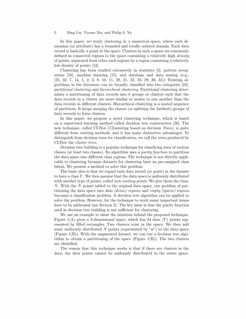
We use an example to show the intuition behind the proposed technique.Figure 1(A) gives a 2-dimensional space, which has 24 data (Y ) points rep-resented by filled rectangles. Two clusters exist in the space. We then addsome uniformly distributed N points (represented by ”o”) to the data space(Figure 1(B)). With the augmented dataset, we can run a decision tree algo-rithm to obtain a partitioning of the space (Figure 1(B)). The two clustersare identified.

The reason that this technique works is that if there are clusters in thedata, the data points cannot be uniformly distributed in the entire space.

Clustering Via Decision Tree Construction 3

Fig. 1. Clustering using decision trees: an intuitive example

By adding some uniformly distributed N points, we can isolate the clustersbecause within each cluster region there are more Y points than N points.The decision tree technique is well known for this task.

We now answer two immediate questions: (1) how many N points shouldwe add, and (2) can the same task be performed without physically adding theN points to the data? The answer to the first question is that it depends. Thenumber changes as the tree grows. It is insufficient to add a fixed number of Npoints to the original dataset at the beginning (see Section 2.2). The answerto the second question is yes. Physically adding N points increases the sizeof the dataset and also the running time. A subtle but important issue isthat it is unlikely that we can have points truly uniformly distributed in avery high dimensional space because we would need an exponential numberof points [23]. We propose a technique to solve the problem, which guaranteesthe uniform distribution of the N points. This is done by not adding anyN point to the space but computing them when needed. Hence, CLTree canproduce the partition in Figure 1(C) with no N point added to the originaldata.

The proposed CLTree technique consists of two steps:

1. Cluster tree construction: This step uses a modified decision tree algorithmwith a new purity function to construct a cluster tree to capture thenatural distribution of the data without making any prior assumptions.

2. Cluster tree pruning: After the tree is built, an interactive pruning stepis performed to simplify the tree to find meaningful/useful clusters. Thefinal clusters are expressed as a list of hyper-rectangular regions.

The rest of the paper develops the idea further. Experiment results on bothsynthetic data and real-life application data show that the proposed techniqueis very effective and scales well for large high dimensional datasets.

1.1 Our contributions

The main contribution of this paper is that it proposes a novel clusteringtechnique, which is based on a supervised learning method [26]. It is fun-damentally different from existing clustering techniques. Existing techniques


form clusters explicitly by grouping data points using some distance or den-sity measures. The proposed technique, however, finds clusters implicitly byseparating data and empty (sparse) regions using a purity function based onthe information theory (the detailed comparison with related work appears inSection 5). The new method has many distinctive advantages over the existingmethods (although some existing methods also have some of the advantages,there is no system that has all the advantages):

• CLTree is able to find clusters without making any prior assumptions orusing any input parameters. Most existing methods require the user tospecify the number of clusters to be found and/or density thresholds (e.g.,[25, 32, 21, 7, 14, 1, 2, 3, 10, 23]). Such values are normally difficult toprovide, and can be quite arbitrary. As a result, the clusters found maynot reflect the ”true” grouping structure of the data.

• CLTree is able to find clusters in the full dimension space as well as inany subspaces. It is noted in [3] that many algorithms that work in thefull space do not work well in subspaces of a high dimensional space. Theopposite is also true, i.e., existing subspace clustering algorithms only findclusters in low dimension subspaces [1, 2, 3]. Our technique is suitablefor both types of clustering because it aims to find simple descriptions ofthe data (using as fewer dimensions as possible), which may use all thedimensions or any subset.

• It provides descriptions of the resulting clusters in terms of hyper-rectangleregions. Most existing clustering methods only group data points togetherand give a centroid for each cluster with no detailed description. Sincedata mining applications typically require descriptions that can be easilyassimilated by the user as insight and explanations, interpretability ofclustering results is of critical importance.

• It comes with an important by-product, the empty (sparse) regions. Al-though clusters are important, empty regions can also be useful. For exam-ple, in a marketing application, clusters may represent different segmentsof existing customers of a company, while the empty regions are the profilesof non-customers. Knowing the profiles of non-customers allows the com-pany to probe into the possibilities of modifying the services or productsand/or of doing targeted marketing in order to attract these potentialcustomers. Sparse regions also reveal outliers and anomalies, which areimportant for many applications.

• It deals with outliers effectively. Outliers are data points in a relativelyempty region. CLTree is able to separate outliers from real clusters be-cause it naturally identifies sparse and dense regions. When outliers areconcentrated in certain areas, it is possible that they will be identified assmall clusters. If such outlier clusters are undesirable, we can use a simplethreshold on the size of clusters to remove them. However, sometimes suchsmall clusters can be very useful as they may represent exceptions (or un-


expected cases) in the data. The interpretation of these small clusters isdependent on applications.

2 Building Cluster Trees

This section presents our cluster tree algorithm. Since a cluster tree is basicallya decision tree for clustering, we first review the decision tree algorithm in [26].We then modify the algorithm and its purity function for clustering.

2.1 Decision tree construction

Decision tree construction is a well-known technique for classification [26].A database for decision tree classification consists of a set of data records,which are pre-classified into q(≥ 2) known classes. The objective of decisiontree construction is to partition the data to separate the q classes. A decisiontree has two types of nodes, decision nodes and leaf nodes. A decision nodespecifies some test on a single attribute. A leaf node indicates the class.

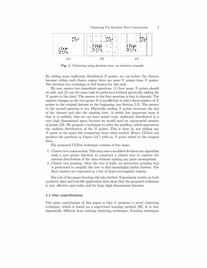
From a geometric point of view, a decision tree represents a partitioningof the data space. A serial of tests (or cuts) from the root node to a leaf noderepresents a hyper-rectangle. For example, the four hyper-rectangular regionsin Figure 2(A) are produced by the tree in Figure 2(B). A region representedby a leaf can also be expressed as a rule, e.g., the upper right region in Figure2(A) can be represented by X > 3.5, Y > 3.5 → O, which is also the rightmost leaf in Figure 2(B). Note that for a numeric attribute, the decision treealgorithm in [26] performs binary split, i.e., each cut splits the current spaceinto two parts (see Figure 2(B)).

Fig. 2. An example partition of the data space and its corresponding decision tree

The algorithm for building a decision tree typically uses the divide andconquer strategy to recursively partition the data to produce the tree. Eachsuccessive step greedily chooses the best cut to partition the space into two


parts in order to obtain purer regions. A commonly used criterion (or purityfunction) for choosing the best cut is the information gain [26]4.

The information gain criterion is derived from information theory. Theessential idea of information theory is that the information conveyed by amessage depends on its probability and can be measured in bits as minus thelogarithm to base 2 of that probability.

Suppose we have a dataset D with q classes, C1, ..., Cq. Suppose furtherthat we have a possible test x with m outcomes that partitions D into msubsets D1, ..., Dm. For a numeric attribute, m = 2, since we only performbinary split. The probability that we select one record from the set D of datarecords and announce that it belongs to some class Cj is given by:

freq(Cj , D)|D|

where freq(Cj , D) represents the number of data records (points) of the classCj in D, while |D| is the total number of data records in D. So the informationthat it conveys is:

− log2

(freq (Cj , D)

|D|)

bits

To find the expected information needed to identify the class of a data recordin D before partitioning occurs, we sum over the classes in proportion to theirfrequencies in D, giving:

info(D) = −q∑

j=1

freq(Cj , D)|D| × log2

(freq(Cj , D)

|D|)

Now, suppose that the dataset D has been partitioned in accordance with them outcomes of the test X. The expected amount of information needed toidentify the class of a data record in D after the partitioning had occurredcan be found as the weighted sum over the subsets, as:

infoX(D) = −m∑

i=1

|Di||D| × info(Di)

where |Di| represents the number of data records in the subset Di after thepartitioning had occurred. The information gained due to the partition is:

gain(X) = info(D)− infoX(D)

Clearly, we should maximize the gain. The gain criterion is to select the testor cut that maximizes the gain to partition the current data (or space).

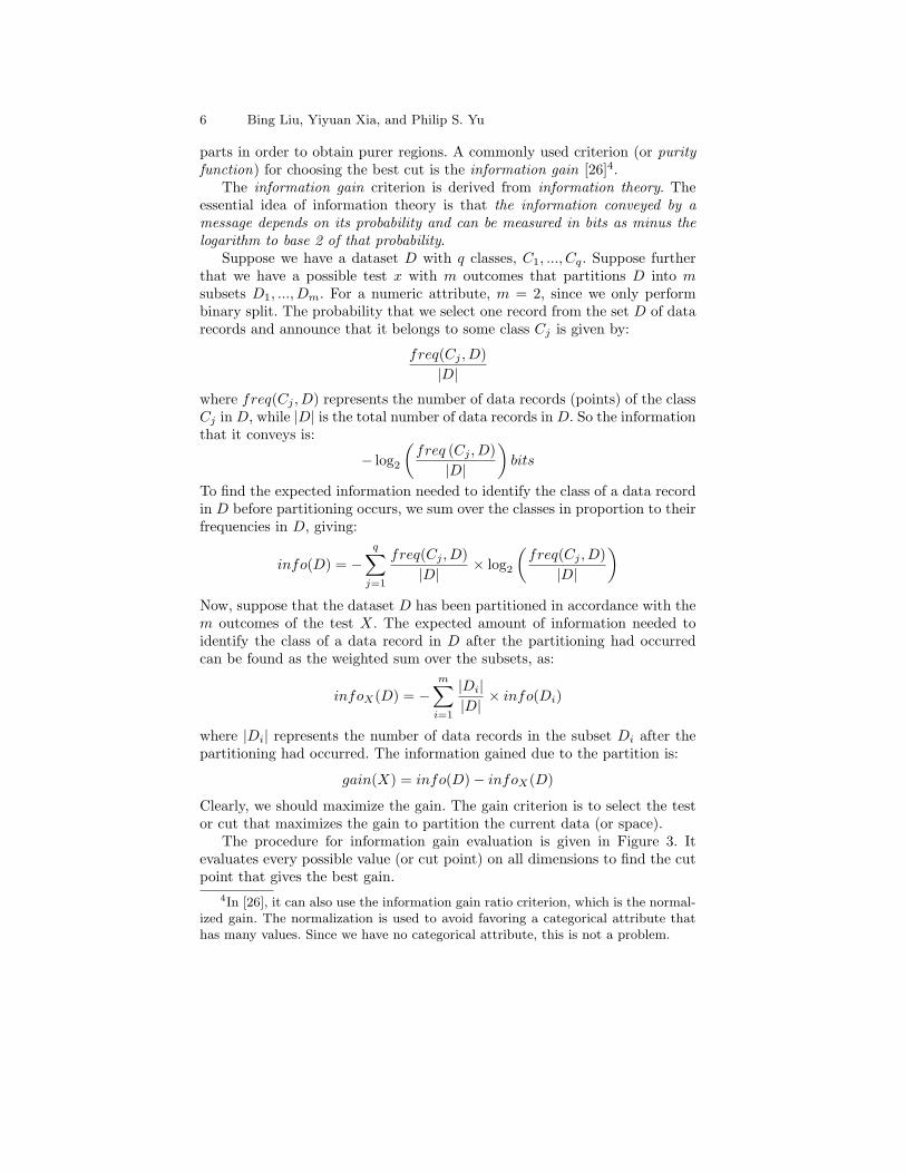
The procedure for information gain evaluation is given in Figure 3. Itevaluates every possible value (or cut point) on all dimensions to find the cutpoint that gives the best gain.

4In [26], it can also use the information gain ratio criterion, which is the normal-ized gain. The normalization is used to avoid favoring a categorical attribute thathas many values. Since we have no categorical attribute, this is not a problem.


1 for each attribute Ai ∈ {A1, A2, , Ad} do/* A1, A2, ,and Ad are the attributes of D */

2 for each value x of Ai in D do/* each value is considered as a possible cut */

3 compute the information gain at x4 end5 end6 Select the test or cut that gives the best information gain to partition the

space

Fig. 3. The information gain evaluation

Scale-up decision tree algorithms: Traditionally, a decision tree al-gorithm requires the whole data to reside in memory. When the dataset istoo large, techniques from the database community can be used to scale upthe algorithm so that the entire dataset is not required in memory. [4] intro-duces an interval classifier that uses data indices to efficiently retrieve portionsof data. SPRINT [27] and RainForest [18] propose two scalable techniquesfor decision tree building. For example, RainForest only keeps an AVC-set(attribute-value, classLabel and count) for each attribute in memory. This issufficient for tree building and gain evaluation. It eliminates the need to havethe entire dataset in memory. BOAT [19] uses statistical techniques to con-struct the tree based on a small subset of the data, and correct inconsistencydue to sampling via a scan over the database.

2.2 Building cluster trees: Introducing N points

We now present the modifications made to the decision tree algorithm in [26]for our clustering purpose. This sub-section focuses on introducing N points.The next sub-section discusses two changes that need to be made to thedecision tree algorithm. The final sub-section describes the new cut selectioncriterion or purity function.

As mentioned before, we give each data point in the original dataset theclass Y , and introduce some uniformly distributed ”non-existing” N points.We do not physically add these N points to the original data, but only assumetheir existence.

We now determine how many N points to add. We add a different numberof N points at each node in tree building. The number of N points for thecurrent node E is determined by the following rule (note that at the rootnode, the number of inherited N points is 0):

1 If the number of N points inherited from the parent node of E is lessthan the number of Y points in E then

2 the number of N points for E is increased to the number of Ypoints in E

3 else the number of inherited N points from its parent is used for E


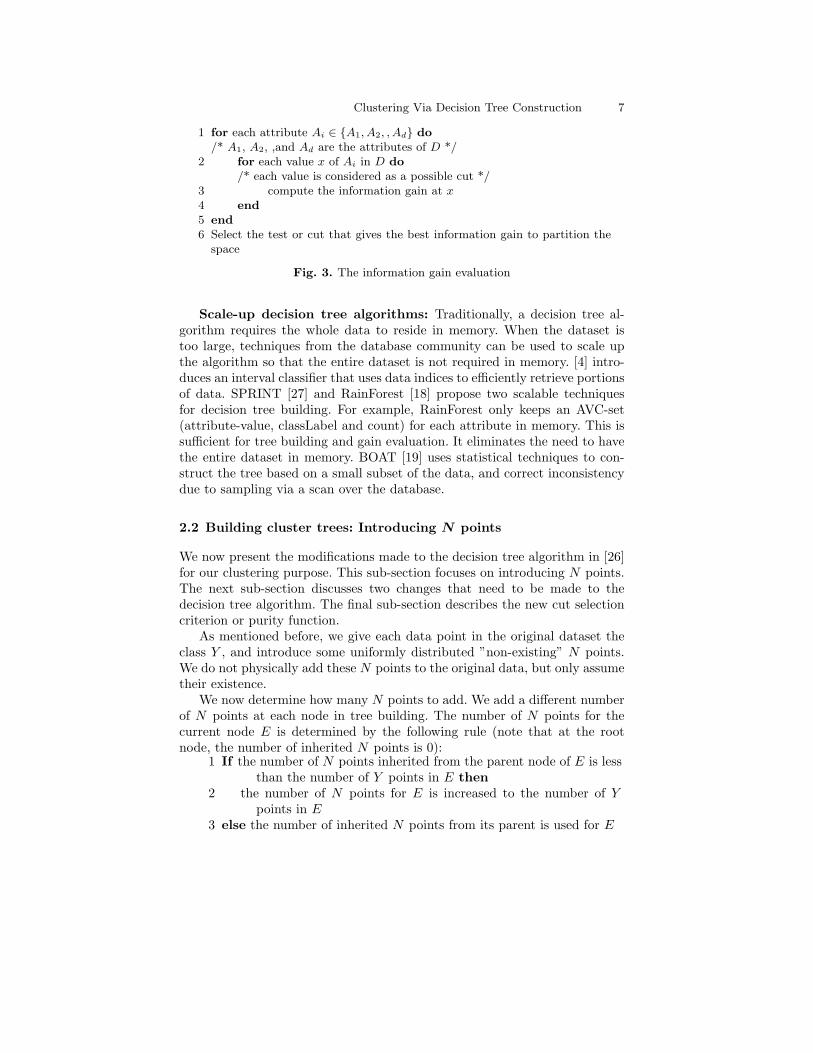
Figure 4 gives an example. The (parent) node P has two children nodes Land R. Assume P has 1000 Y points and thus 1000 N points, stored in P.Yand P.N respectively. Assume after splitting, L has 20 Y points and 500 Npoints, and R has 980 Y points and 500 N points. According to the aboverule, for subsequent partitioning, we increase the number of N points at R to980. The number of N points at L is unchanged.

Fig. 4. Distributing N pointsFig. 5. The effect of using a fixed numberof N points

The basic idea is that we use an equal number of N points to the numberof Y (data) points (in fact, 1:1 ratio is not necessary, see Section 4.2.2). This isnatural because it allows us to isolate those regions that are densely populatedwith data points. The reason that we increase the number of N points of anode (line 2) if it has more inherited Y points than N points is to avoid thesituation where there may be too few N points left after some cuts or splits.If we fix the number of N points in the entire space to be the number of Ypoints in the original data, the number of N points at a later node can easilydrop to a very small number for a high dimensional space. If there are too fewN points, further splits become difficult, but such splits may still be necessary.Figure 5 gives an example.

In Figure 5, the original space contains 32 data (Y ) points. Accordingto the above rule, it also has 32 N points. After two cuts, we are left witha smaller region (region 1). All the Y points are in this region. If we donot increase the number of N points for the region, we are left with only32/22 = 8 N points in region 1. This is not so bad because the space has onlytwo dimensions. If we have a very high dimensional space, the number of Npoints will drop drastically (close to 0) after some splits (as the number of Npoints drops exponentially).

The number of N points is not reduced if the current node is an N node(an N node has more N points than Y points) (line 3). A reduction may causeoutlier Y points to form Y nodes or regions (a Y node has an equal number ofY points as N points or more). Then cluster regions and non-cluster regionsmay not be separated.


2.3 Building cluster trees: Two modifications to the decision treealgorithm

Since the N points are not physically added to the data, we need to make twomodifications to the decision tree algorithm in [26] in order to build clustertrees:

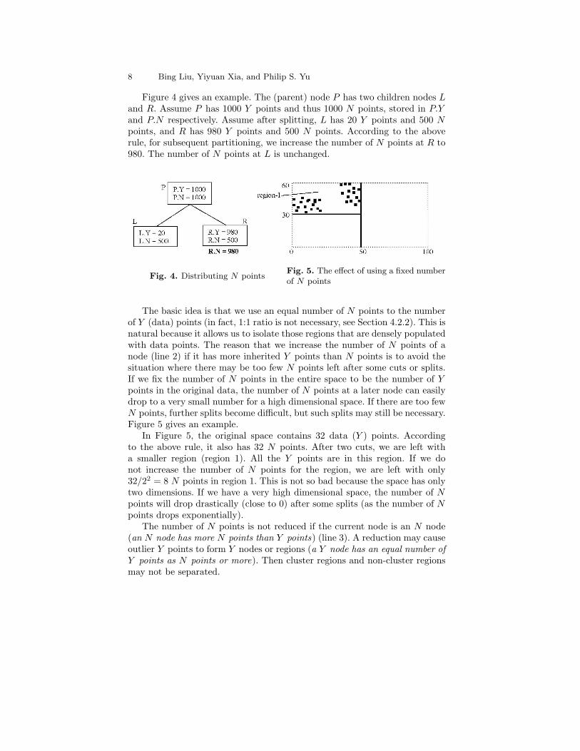
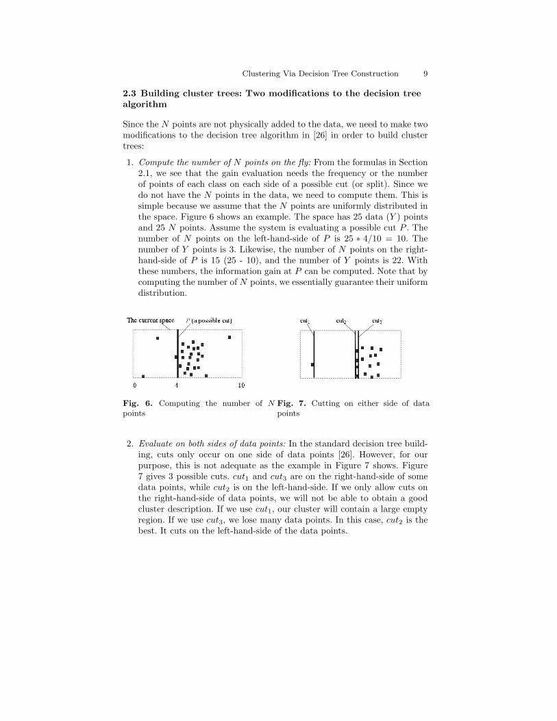
1. Compute the number of N points on the fly: From the formulas in Section2.1, we see that the gain evaluation needs the frequency or the numberof points of each class on each side of a possible cut (or split). Since wedo not have the N points in the data, we need to compute them. This issimple because we assume that the N points are uniformly distributed inthe space. Figure 6 shows an example. The space has 25 data (Y ) pointsand 25 N points. Assume the system is evaluating a possible cut P . Thenumber of N points on the left-hand-side of P is 25 ∗ 4/10 = 10. Thenumber of Y points is 3. Likewise, the number of N points on the right-hand-side of P is 15 (25 - 10), and the number of Y points is 22. Withthese numbers, the information gain at P can be computed. Note that bycomputing the number of N points, we essentially guarantee their uniformdistribution.

Fig. 6. Computing the number of Npoints

Fig. 7. Cutting on either side of datapoints

2. Evaluate on both sides of data points: In the standard decision tree build-ing, cuts only occur on one side of data points [26]. However, for ourpurpose, this is not adequate as the example in Figure 7 shows. Figure7 gives 3 possible cuts. cut1 and cut3 are on the right-hand-side of somedata points, while cut2 is on the left-hand-side. If we only allow cuts onthe right-hand-side of data points, we will not be able to obtain a goodcluster description. If we use cut1, our cluster will contain a large emptyregion. If we use cut3, we lose many data points. In this case, cut2 is thebest. It cuts on the left-hand-side of the data points.


2.4 Building cluster trees: The new criterion for selecting the bestcut

Decision tree building for classification uses the gain criterion to select thebest cut. For clustering, this is insufficient. The cut that gives the best gainmay not be the best cut for clustering. There are two main problems with thegain criterion:

1. The cut with the best information gain tends to cut into clusters.2. The gain criterion does not look ahead in deciding the best cut.

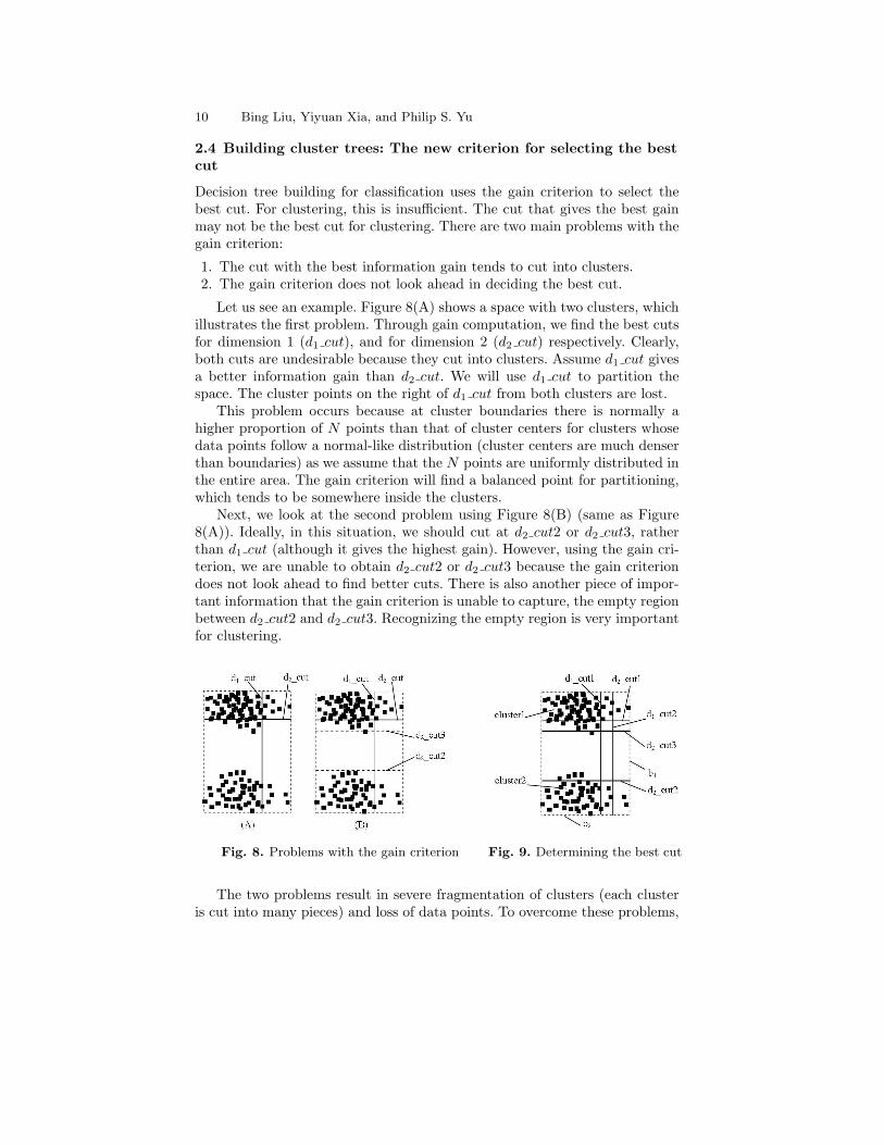
Let us see an example. Figure 8(A) shows a space with two clusters, whichillustrates the first problem. Through gain computation, we find the best cutsfor dimension 1 (d1 cut), and for dimension 2 (d2 cut) respectively. Clearly,both cuts are undesirable because they cut into clusters. Assume d1 cut givesa better information gain than d2 cut. We will use d1 cut to partition thespace. The cluster points on the right of d1 cut from both clusters are lost.

This problem occurs because at cluster boundaries there is normally ahigher proportion of N points than that of cluster centers for clusters whosedata points follow a normal-like distribution (cluster centers are much denserthan boundaries) as we assume that the N points are uniformly distributed inthe entire area. The gain criterion will find a balanced point for partitioning,which tends to be somewhere inside the clusters.

Next, we look at the second problem using Figure 8(B) (same as Figure8(A)). Ideally, in this situation, we should cut at d2 cut2 or d2 cut3, ratherthan d1 cut (although it gives the highest gain). However, using the gain cri-terion, we are unable to obtain d2 cut2 or d2 cut3 because the gain criteriondoes not look ahead to find better cuts. There is also another piece of impor-tant information that the gain criterion is unable to capture, the empty regionbetween d2 cut2 and d2 cut3. Recognizing the empty region is very importantfor clustering.

Fig. 8. Problems with the gain criterion Fig. 9. Determining the best cut

The two problems result in severe fragmentation of clusters (each clusteris cut into many pieces) and loss of data points. To overcome these problems,


we designed a new criterion, which still uses information gain as the basis, butadds to it the ability to look ahead. We call the new criterion the lookaheadgain criterion. For the example in Figure 8(B), we aim to find a cut that isvery close to d2 cut2 or d2 cut3.

The basic idea is as follows: For each dimension i, based on the first cutfound using the gain criterion, we look ahead (at most 2 steps) along eachdimension to find a better cut ci that cuts less into cluster regions, and to findan associated region ri that is relatively empty (measured by relative density,see below). ci of the dimension i whose ri has the lowest relative density isselected as the best cut. The intuition behind this modified criterion is clear.It tries to find the emptiest region along each dimension to separate clusters.

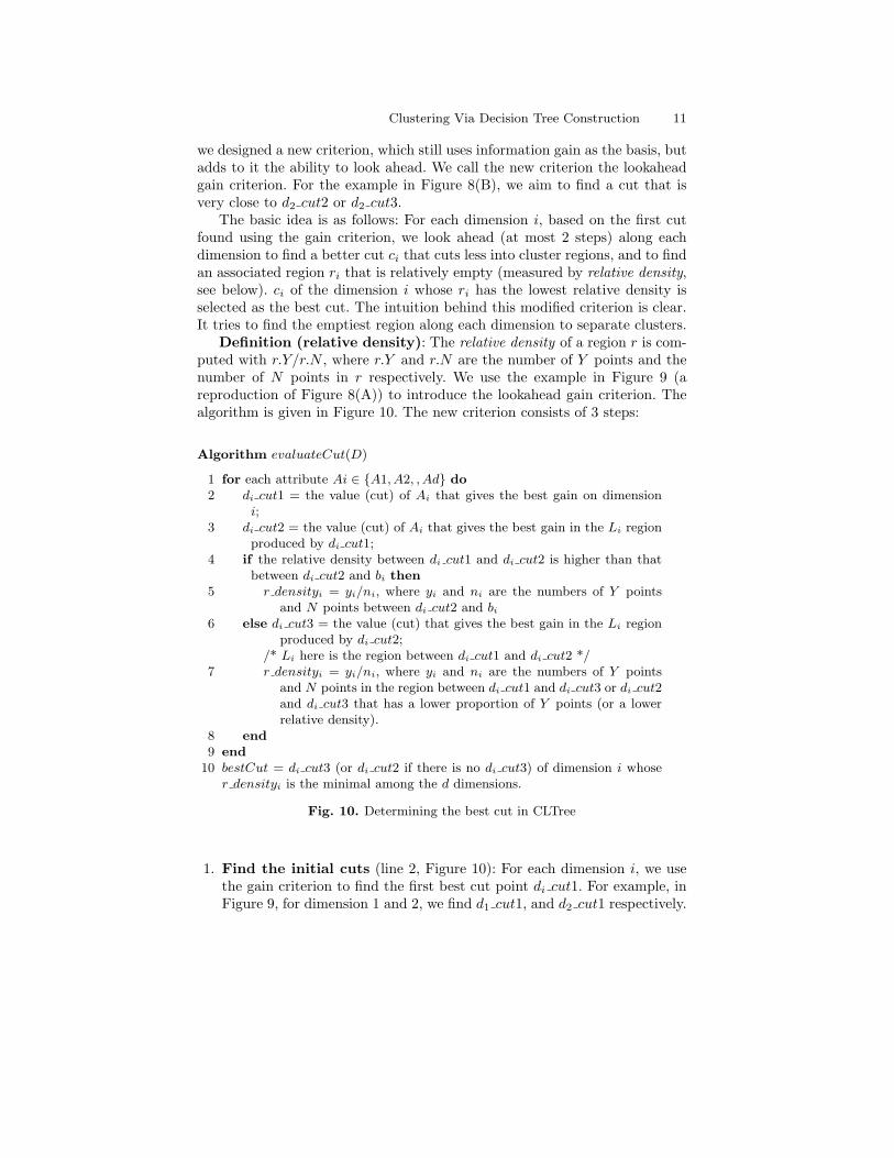
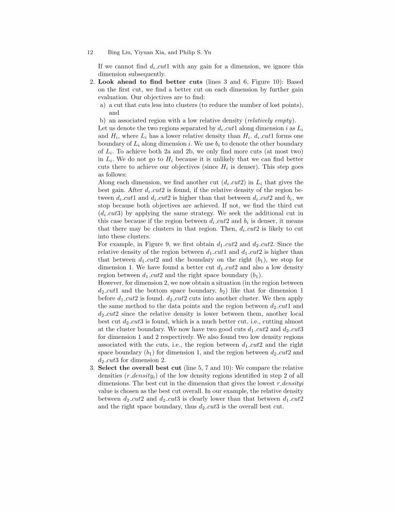
Definition (relative density): The relative density of a region r is com-puted with r.Y/r.N , where r.Y and r.N are the number of Y points and thenumber of N points in r respectively. We use the example in Figure 9 (areproduction of Figure 8(A)) to introduce the lookahead gain criterion. Thealgorithm is given in Figure 10. The new criterion consists of 3 steps:

Algorithm evaluateCut(D)

1 for each attribute Ai ∈ {A1, A2, , Ad} do2 di cut1 = the value (cut) of Ai that gives the best gain on dimension

i;3 di cut2 = the value (cut) of Ai that gives the best gain in the Li region

produced by di cut1;4 if the relative density between di cut1 and di cut2 is higher than that

between di cut2 and bi then5 r densityi = yi/ni, where yi and ni are the numbers of Y points

and N points between di cut2 and bi

6 else di cut3 = the value (cut) that gives the best gain in the Li regionproduced by di cut2;

/* Li here is the region between di cut1 and di cut2 */7 r densityi = yi/ni, where yi and ni are the numbers of Y points

and N points in the region between di cut1 and di cut3 or di cut2and di cut3 that has a lower proportion of Y points (or a lowerrelative density).

8 end9 end

10 bestCut = di cut3 (or di cut2 if there is no di cut3) of dimension i whoser densityi is the minimal among the d dimensions.

Fig. 10. Determining the best cut in CLTree

1. Find the initial cuts (line 2, Figure 10): For each dimension i, we usethe gain criterion to find the first best cut point di cut1. For example, inFigure 9, for dimension 1 and 2, we find d1 cut1, and d2 cut1 respectively.


If we cannot find di cut1 with any gain for a dimension, we ignore thisdimension subsequently.

2. Look ahead to find better cuts (lines 3 and 6, Figure 10): Basedon the first cut, we find a better cut on each dimension by further gainevaluation. Our objectives are to find:a) a cut that cuts less into clusters (to reduce the number of lost points),

andb) an associated region with a low relative density (relatively empty).Let us denote the two regions separated by di cut1 along dimension i as Li

and Hi, where Li has a lower relative density than Hi. di cut1 forms oneboundary of Li along dimension i. We use bi to denote the other boundaryof Li. To achieve both 2a and 2b, we only find more cuts (at most two)in Li. We do not go to Hi because it is unlikely that we can find bettercuts there to achieve our objectives (since Hi is denser). This step goesas follows:Along each dimension, we find another cut (di cut2) in Li that gives thebest gain. After di cut2 is found, if the relative density of the region be-tween di cut1 and di cut2 is higher than that between di cut2 and bi, westop because both objectives are achieved. If not, we find the third cut(di cut3) by applying the same strategy. We seek the additional cut inthis case because if the region between di cut2 and bi is denser, it meansthat there may be clusters in that region. Then, di cut2 is likely to cutinto these clusters.For example, in Figure 9, we first obtain d1 cut2 and d2 cut2. Since therelative density of the region between d1 cut1 and d1 cut2 is higher thanthat between d1 cut2 and the boundary on the right (b1), we stop fordimension 1. We have found a better cut d1 cut2 and also a low densityregion between d1 cut2 and the right space boundary (b1).However, for dimension 2, we now obtain a situation (in the region betweend2 cut1 and the bottom space boundary, b2) like that for dimension 1before d1 cut2 is found. d2 cut2 cuts into another cluster. We then applythe same method to the data points and the region between d2 cut1 andd2 cut2 since the relative density is lower between them, another localbest cut d2 cut3 is found, which is a much better cut, i.e., cutting almostat the cluster boundary. We now have two good cuts d1 cut2 and d2 cut3for dimension 1 and 2 respectively. We also found two low density regionsassociated with the cuts, i.e., the region between d1 cut2 and the rightspace boundary (b1) for dimension 1, and the region between d2 cut2 andd2 cut3 for dimension 2.

3. Select the overall best cut (line 5, 7 and 10): We compare the relativedensities (r densityi) of the low density regions identified in step 2 of alldimensions. The best cut in the dimension that gives the lowest r densityivalue is chosen as the best cut overall. In our example, the relative densitybetween d2 cut2 and d2 cut3 is clearly lower than that between d1 cut2and the right space boundary, thus d2 cut3 is the overall best cut.


The reason that we use relative density to select the overall best cut isbecause it is desirable to split at the cut point that may result in a bigempty (N) region (e.g., between d2 cut2 and d2 cut3), which is more likelyto separate clusters.This algorithm can also be scaled up using the existing decision tree scale-up techniques in [18, 27] since the essential computation here is the sameas that in decision tree building, i.e., the gain evaluation. Our new criterionsimply performs the gain evaluation more than once.

3 User-Oriented Pruning of Cluster Trees

The recursive partitioning method of building cluster trees will divide thedata space until each partition contains only points of a single class, or untilno test (or cut) offers any improvement5 . The result is often a very complextree that partitions the space more than necessary. This problem is the sameas that in classification [26]. There are basically two ways to produce simplertrees:

1. Stopping: deciding not to divide a region any further, or2. Pruning: removing some of the tree parts after the tree has been built.

The first approach has the attraction that time is not wasted in building thecomplex tree. However, it is known in classification research that stoppingis often unreliable because it is very hard to get the stopping criterion right[26]. This has also been our experience. Thus, we adopted the pruning strategy.Pruning is more reliable because after tree building we have seen the completestructure of data. It is much easier to decide which parts are unnecessary.

The pruning method used for classification, however, cannot be appliedhere because clustering, to certain extent, is a subjective task. Whether aclustering is good or bad depends on the application and the user’s subjec-tive judgment of its usefulness [9, 24]. Thus, we use a subjective measure forpruning. We use the example in Figure 11 to explain.

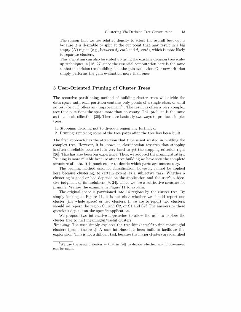
The original space is partitioned into 14 regions by the cluster tree. Bysimply looking at Figure 11, it is not clear whether we should report onecluster (the whole space) or two clusters. If we are to report two clusters,should we report the region C1 and C2, or S1 and S2? The answers to thesequestions depend on the specific application.

We propose two interactive approaches to allow the user to explore thecluster tree to find meaningful/useful clusters.Browsing : The user simply explores the tree him/herself to find meaningfulclusters (prune the rest). A user interface has been built to facilitate thisexploration. This is not a difficult task because the major clusters are identified

5We use the same criterion as that in [26] to decide whether any improvementcan be made.


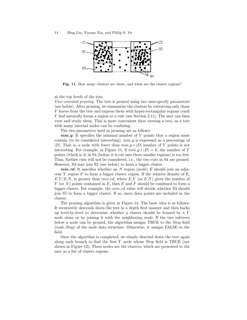
Fig. 11. How many clusters are there, and what are the cluster regions?

at the top levels of the tree.User-oriented pruning : The tree is pruned using two user-specify parameters(see below). After pruning, we summarize the clusters by extracting only thoseY leaves from the tree and express them with hyper-rectangular regions (eachY leaf naturally forms a region or a rule (see Section 2.1)). The user can thenview and study them. This is more convenient then viewing a tree, as a treewith many internal nodes can be confusing.

The two parameters used in pruning are as follows:min y : It specifies the minimal number of Y points that a region must

contain (to be considered interesting). min y is expressed as a percentage of|D|. That is, a node with fewer than min y ∗ |D| number of Y points is notinteresting. For example, in Figure 11, if min y ∗ |D| = 6, the number of Ypoints (which is 4) in S4 (before it is cut into three smaller regions) is too few.Thus, further cuts will not be considered, i.e., the two cuts in S4 are pruned.However, S4 may join S2 (see below) to form a bigger cluster.

min rd : It specifies whether an N region (node) E should join an adja-cent Y region F to form a bigger cluster region. If the relative density of E,E.Y/E.N , is greater than min rd, where E.Y (or E.N) gives the number ofY (or N) points contained in E, then E and F should be combined to form abigger cluster. For example, the min rd value will decide whether S3 shouldjoin S1 to form a bigger cluster. If so, more data points are included in thecluster.

The pruning algorithm is given in Figure 12. The basic idea is as follows:It recursively descends down the tree in a depth first manner and then backsup level-by-level to determine whether a cluster should be formed by a Ynode alone or by joining it with the neighboring node. If the two subtreesbelow a node can be pruned, the algorithm assigns TRUE to the Stop field(node.Stop) of the node data structure. Otherwise, it assigns FALSE to thefield.

Once the algorithm is completed, we simply descend down the tree againalong each branch to find the first Y node whose Stop field is TRUE (notshown in Figure 12). These nodes are the clusters, which are presented to theuser as a list of cluster regions.


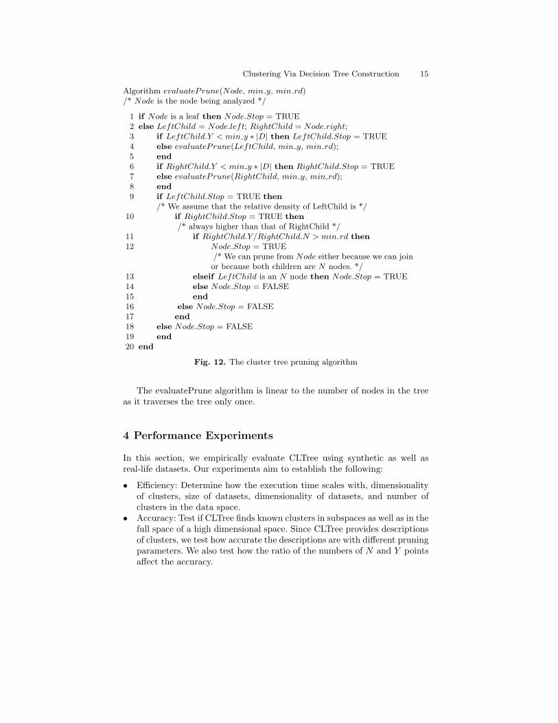
Algorithm evaluatePrune(Node, min y, min rd)/* Node is the node being analyzed */

1 if Node is a leaf then Node.Stop = TRUE2 else LeftChild = Node.left; RightChild = Node.right;3 if LeftChild.Y < min y ∗ |D| then LeftChild.Stop = TRUE4 else evaluatePrune(LeftChild, min y, min rd);5 end6 if RightChild.Y < min y ∗ |D| then RightChild.Stop = TRUE7 else evaluatePrune(RightChild, min y, min rd);8 end9 if LeftChild.Stop = TRUE then

/* We assume that the relative density of LeftChild is */10 if RightChild.Stop = TRUE then

/* always higher than that of RightChild */11 if RightChild.Y/RightChild.N > min rd then12 Node.Stop = TRUE

/* We can prune from Node either because we can joinor because both children are N nodes. */

13 elseif LeftChild is an N node then Node.Stop = TRUE14 else Node.Stop = FALSE15 end16 else Node.Stop = FALSE17 end18 else Node.Stop = FALSE19 end20 end

Fig. 12. The cluster tree pruning algorithm

The evaluatePrune algorithm is linear to the number of nodes in the treeas it traverses the tree only once.

4 Performance Experiments

In this section, we empirically evaluate CLTree using synthetic as well asreal-life datasets. Our experiments aim to establish the following:

• Efficiency: Determine how the execution time scales with, dimensionalityof clusters, size of datasets, dimensionality of datasets, and number ofclusters in the data space.

• Accuracy: Test if CLTree finds known clusters in subspaces as well as in thefull space of a high dimensional space. Since CLTree provides descriptionsof clusters, we test how accurate the descriptions are with different pruningparameters. We also test how the ratio of the numbers of N and Y pointsaffect the accuracy.


All the experiments were run on SUN E450 with one 250MHZ cpu and 512MBmemory.

4.1 Synthetic data generation

We implemented two data generators for our experiments. One generatesdatasets following a normal distribution, and the other generates datasetsfollowing a uniform distribution. For both generators, all data points havecoordinates in the range [0, 100] on each dimension. The percentage of noiseor outliers (noise level) is a parameter. Outliers are distributed uniformly atrandom throughout the entire space.

Normal distribution: The first data generator generates data points ineach cluster following a normal distribution. Each cluster is described by thesubset of dimensions, the number of data points, and the value range alongeach cluster dimension. The data points for a given cluster are generated asfollows: The coordinates of the data points on the non-cluster dimensions aregenerated uniformly at random. For a cluster dimension, the coordinates ofthe data points projected onto the dimension follow a normal distribution.The data generator is able to generate clusters of elliptical shape and also hasthe flexibility to generate clusters of different sizes.

Uniform distribution: The second data generator generates data pointsin each cluster following a uniform distribution. The clusters are hyper-rectangles in a subset (including the full set) of the dimensions. The surfacesof such a cluster are parallel to axes. The data points for a given cluster aregenerated as follows: The coordinates of the data points on non-cluster di-mensions are generated uniformly at random over the entire value ranges ofthe dimensions. For a cluster dimension in the subspace in which the cluster isembedded, the value is drawn at random from a uniform distribution withinthe specified value range.

4.2 Synthetic data results

Scalability results

For our experiments reported below, the noise level is set at 10%. The execu-tion times (in sec.) do not include the time for pruning, but only tree building.Pruning is very efficient because we only need to traverse the tree once. Thedatasets reside in memory.

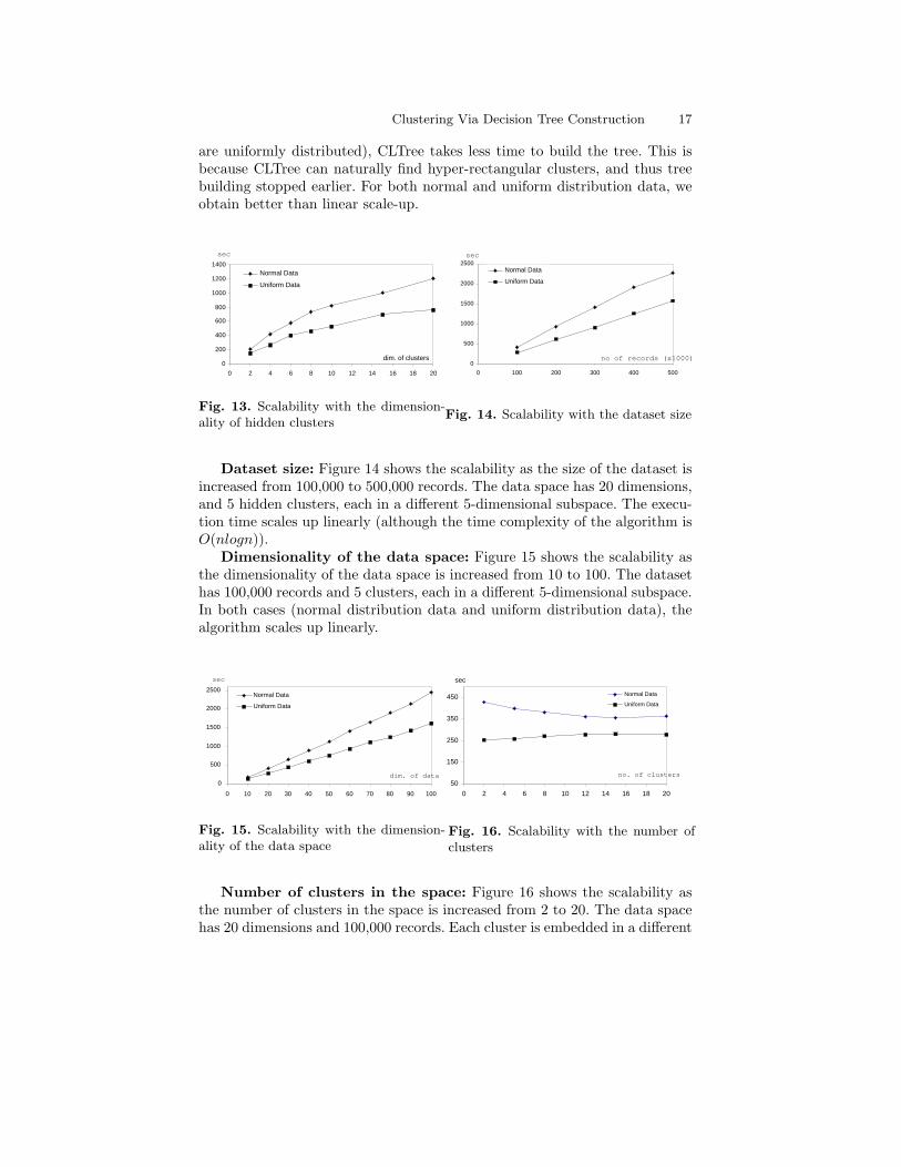
Dimensionality of hidden clusters: CLTree can be used for findingclusters in the full dimensional space as well as in any subspaces. Figure 13shows the scalability as the dimensionality of the clusters is increased from2 to 20 in a 20-dimensional space. In each case, 5 clusters are embedded indifferent subspaces of the 20-dimensional space. In the last case, the clustersare in the full space. Each dataset has 100,000 records. From the figure, wesee that when the clusters are hyper-rectangles (in which the data points


are uniformly distributed), CLTree takes less time to build the tree. This isbecause CLTree can naturally find hyper-rectangular clusters, and thus treebuilding stopped earlier. For both normal and uniform distribution data, weobtain better than linear scale-up.

0

500

1000

1500

2000

2500

0 100 200 300 400 500

Normal Data

Uniform Data

sec

no of records (x1000) 0

200

400

600

800

1000

1200

1400

0 2 4 6 8 10 12 14 16 18 20

Normal Data

Uniform Data

dim. of clusters

sec

Fig. 13. Scalability with the dimension-ality of hidden clusters

Fig. 14. Scalability with the dataset size

Dataset size: Figure 14 shows the scalability as the size of the dataset isincreased from 100,000 to 500,000 records. The data space has 20 dimensions,and 5 hidden clusters, each in a different 5-dimensional subspace. The execu-tion time scales up linearly (although the time complexity of the algorithm isO(nlogn)).

Dimensionality of the data space: Figure 15 shows the scalability asthe dimensionality of the data space is increased from 10 to 100. The datasethas 100,000 records and 5 clusters, each in a different 5-dimensional subspace.In both cases (normal distribution data and uniform distribution data), thealgorithm scales up linearly.

0

500

1000

1500

2000

2500

0 10 20 30 40 50 60 70 80 90 100

Normal Data

Uniform Data

dim. of data

sec

50

150

250

350

450

0 2 4 6 8 10 12 14 16 18 20

Normal Data

Uniform Data

sec

no. of clusters

Fig. 15. Scalability with the dimension-ality of the data space

Fig. 16. Scalability with the number ofclusters

Number of clusters in the space: Figure 16 shows the scalability asthe number of clusters in the space is increased from 2 to 20. The data spacehas 20 dimensions and 100,000 records. Each cluster is embedded in a different


5-dimensional subspace. For both uniform and normal datasets, the executiontimes do not vary a great deal as the number of clusters increases.

Accuracy and sensitivity results

In all the above experiments, CLTree recovers all the original clusters em-bedded in the full dimensional space and subspaces. All cluster dimensionsand their boundaries are found without including any extra dimension. Forpruning, we use CLTree’s default settings of min y = 1% and min rd = 10%(see below).

Since CLTree provides precise cluster descriptions, which are representedby hyper-rectangles and the number of data (Y ) points contained in each ofthem, below we show the percentage of data points recovered in the clus-ters using various min y and min rd values, and noise levels. Two sets ofexperiments are conducted. In both sets, each data space has 20 dimensions,and 100,000 data points. In the first set, the number of clusters is 5, andin the other set, the number of clusters is 10. Each cluster is in a different5-dimensional subspace. We will also show how the ratio of N and Y pointsaffects the accuracy.

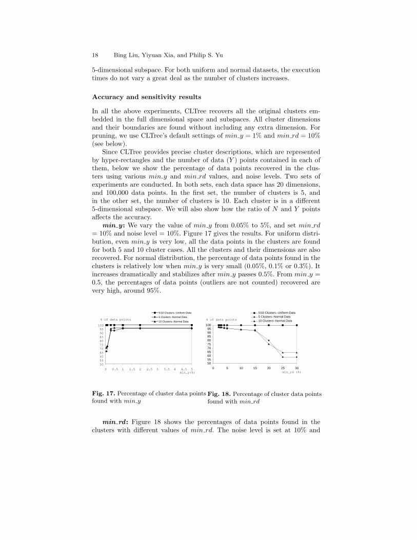
min y : We vary the value of min y from 0.05% to 5%, and set min rd= 10% and noise level = 10%. Figure 17 gives the results. For uniform distri-bution, even min y is very low, all the data points in the clusters are foundfor both 5 and 10 cluster cases. All the clusters and their dimensions are alsorecovered. For normal distribution, the percentage of data points found in theclusters is relatively low when min y is very small (0.05%, 0.1% or 0.3%). Itincreases dramatically and stabilizes after min y passes 0.5%. From min y =0.5, the percentages of data points (outliers are not counted) recovered arevery high, around 95%.

50556065707580859095100

0 0.5 1 1.5 2 2.5 3 3.5 4 4.5 5

5/10 Clusters--Uniform Data

5 Clusters--Normal Data

10 Clusters--Normal Data % of data points

min_y(%)

50 55 60 65 70 75 80 85 90 95

100

0 5 10 15 20 25 30

5/10 Clusters--Uniform Data 5 Clusters--Normal Data 10 Clusters--Normal Data

min_rd (%)

% of data points

Fig. 17. Percentage of cluster data pointsfound with min y

Fig. 18. Percentage of cluster data pointsfound with min rd

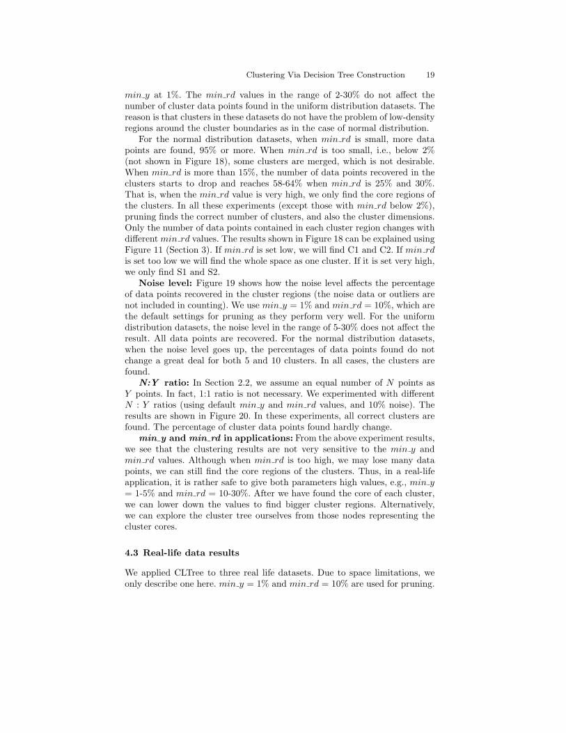
min rd : Figure 18 shows the percentages of data points found in theclusters with different values of min rd. The noise level is set at 10% and


min y at 1%. The min rd values in the range of 2-30% do not affect thenumber of cluster data points found in the uniform distribution datasets. Thereason is that clusters in these datasets do not have the problem of low-densityregions around the cluster boundaries as in the case of normal distribution.

For the normal distribution datasets, when min rd is small, more datapoints are found, 95% or more. When min rd is too small, i.e., below 2%(not shown in Figure 18), some clusters are merged, which is not desirable.When min rd is more than 15%, the number of data points recovered in theclusters starts to drop and reaches 58-64% when min rd is 25% and 30%.That is, when the min rd value is very high, we only find the core regions ofthe clusters. In all these experiments (except those with min rd below 2%),pruning finds the correct number of clusters, and also the cluster dimensions.Only the number of data points contained in each cluster region changes withdifferent min rd values. The results shown in Figure 18 can be explained usingFigure 11 (Section 3). If min rd is set low, we will find C1 and C2. If min rdis set too low we will find the whole space as one cluster. If it is set very high,we only find S1 and S2.

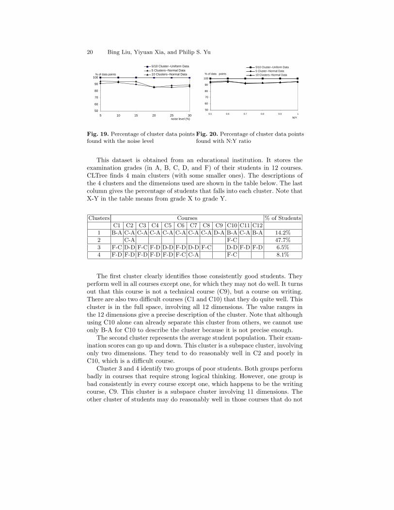
Noise level: Figure 19 shows how the noise level affects the percentageof data points recovered in the cluster regions (the noise data or outliers arenot included in counting). We use min y = 1% and min rd = 10%, which arethe default settings for pruning as they perform very well. For the uniformdistribution datasets, the noise level in the range of 5-30% does not affect theresult. All data points are recovered. For the normal distribution datasets,when the noise level goes up, the percentages of data points found do notchange a great deal for both 5 and 10 clusters. In all cases, the clusters arefound.

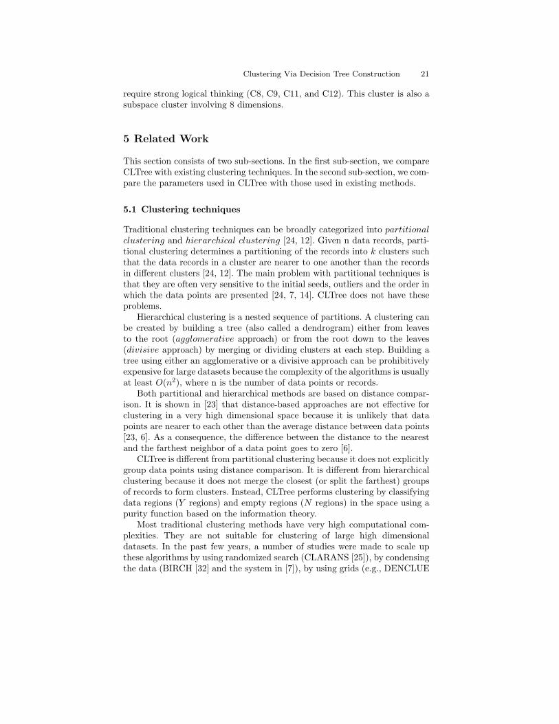
N:Y ratio: In Section 2.2, we assume an equal number of N points asY points. In fact, 1:1 ratio is not necessary. We experimented with differentN : Y ratios (using default min y and min rd values, and 10% noise). Theresults are shown in Figure 20. In these experiments, all correct clusters arefound. The percentage of cluster data points found hardly change.

min y and min rd in applications: From the above experiment results,we see that the clustering results are not very sensitive to the min y andmin rd values. Although when min rd is too high, we may lose many datapoints, we can still find the core regions of the clusters. Thus, in a real-lifeapplication, it is rather safe to give both parameters high values, e.g., min y= 1-5% and min rd = 10-30%. After we have found the core of each cluster,we can lower down the values to find bigger cluster regions. Alternatively,we can explore the cluster tree ourselves from those nodes representing thecluster cores.

4.3 Real-life data results

We applied CLTree to three real life datasets. Due to space limitations, weonly describe one here. min y = 1% and min rd = 10% are used for pruning.


50

60

70

80

90

100

5 10 15 20 25 30

5/10 Cluster--Uniform Data 5 Clusters--Normal Data 10 Clusters--Normal Data

noise level (%)

% of data points

Fig. 19. Percentage of cluster data pointsfound with the noise level

50

60

70

80

90

100

0.5 0.6 0.7 0.8 0.9 1

5/10 Cluster--Uniform Data 5 Cluster--Normal Data 10 Clusters--Normal Data % of data points

N/Y

Fig. 20. Percentage of cluster data pointsfound with N:Y ratio

This dataset is obtained from an educational institution. It stores theexamination grades (in A, B, C, D, and F) of their students in 12 courses.CLTree finds 4 main clusters (with some smaller ones). The descriptions ofthe 4 clusters and the dimensions used are shown in the table below. The lastcolumn gives the percentage of students that falls into each cluster. Note thatX-Y in the table means from grade X to grade Y.

Clusters Courses % of Students

C1 C2 C3 C4 C5 C6 C7 C8 C9 C10 C11 C12

1 B-A C-A C-A C-A C-A C-A C-A C-A D-A B-A C-A B-A 14.2%

2 C-A F-C 47.7%

3 F-C D-D F-C F-D D-D F-D D-D F-C D-D F-D F-D 6.5%

4 F-D F-D F-D F-D F-D F-C C-A F-C 8.1%

The first cluster clearly identifies those consistently good students. Theyperform well in all courses except one, for which they may not do well. It turnsout that this course is not a technical course (C9), but a course on writing.There are also two difficult courses (C1 and C10) that they do quite well. Thiscluster is in the full space, involving all 12 dimensions. The value ranges inthe 12 dimensions give a precise description of the cluster. Note that althoughusing C10 alone can already separate this cluster from others, we cannot useonly B-A for C10 to describe the cluster because it is not precise enough.

The second cluster represents the average student population. Their exam-ination scores can go up and down. This cluster is a subspace cluster, involvingonly two dimensions. They tend to do reasonably well in C2 and poorly inC10, which is a difficult course.

Cluster 3 and 4 identify two groups of poor students. Both groups performbadly in courses that require strong logical thinking. However, one group isbad consistently in every course except one, which happens to be the writingcourse, C9. This cluster is a subspace cluster involving 11 dimensions. Theother cluster of students may do reasonably well in those courses that do not


require strong logical thinking (C8, C9, C11, and C12). This cluster is also asubspace cluster involving 8 dimensions.

5 Related Work

This section consists of two sub-sections. In the first sub-section, we compareCLTree with existing clustering techniques. In the second sub-section, we com-pare the parameters used in CLTree with those used in existing methods.

5.1 Clustering techniques

Traditional clustering techniques can be broadly categorized into partitionalclustering and hierarchical clustering [24, 12]. Given n data records, parti-tional clustering determines a partitioning of the records into k clusters suchthat the data records in a cluster are nearer to one another than the recordsin different clusters [24, 12]. The main problem with partitional techniques isthat they are often very sensitive to the initial seeds, outliers and the order inwhich the data points are presented [24, 7, 14]. CLTree does not have theseproblems.

Hierarchical clustering is a nested sequence of partitions. A clustering canbe created by building a tree (also called a dendrogram) either from leavesto the root (agglomerative approach) or from the root down to the leaves(divisive approach) by merging or dividing clusters at each step. Building atree using either an agglomerative or a divisive approach can be prohibitivelyexpensive for large datasets because the complexity of the algorithms is usuallyat least O(n2), where n is the number of data points or records.

Both partitional and hierarchical methods are based on distance compar-ison. It is shown in [23] that distance-based approaches are not effective forclustering in a very high dimensional space because it is unlikely that datapoints are nearer to each other than the average distance between data points[23, 6]. As a consequence, the difference between the distance to the nearestand the farthest neighbor of a data point goes to zero [6].

CLTree is different from partitional clustering because it does not explicitlygroup data points using distance comparison. It is different from hierarchicalclustering because it does not merge the closest (or split the farthest) groupsof records to form clusters. Instead, CLTree performs clustering by classifyingdata regions (Y regions) and empty regions (N regions) in the space using apurity function based on the information theory.

Most traditional clustering methods have very high computational com-plexities. They are not suitable for clustering of large high dimensionaldatasets. In the past few years, a number of studies were made to scale upthese algorithms by using randomized search (CLARANS [25]), by condensingthe data (BIRCH [32] and the system in [7]), by using grids (e.g., DENCLUE


[22]), and by sampling (CURE [21]). These works are different from ours be-cause our objective is not to scale up an existing algorithm, but to propose anew clustering technique that can overcome many problems with the existingmethods.

Recently, some clustering algorithms based on local density comparisonsand/or grids were reported, e.g., DBSCAN [10], DBCLASD [31], STING [30],WaveCluster [28] and DENCLUE [22]. Density-based approaches, however,are not effective in a high dimensional space because the space is too sparselyfilled (see [23] for more discussions). It is noted in [3] that DBSCAN only runswith datasets having fewer than 10 dimensions. Furthermore, these methodscannot be used to find subspace clusters.

OptiGrid [23] finds clusters in high dimension spaces by projecting thedata onto each axis and then partitioning the data using cutting planes atlow-density points. The approach will not work effectively in situations wheresome well-separated clusters in the full space may overlap when they areprojected onto each axis. OptiGrid also cannot find subspace clusters.

CLIQUE [3] is a subspace clustering algorithm. It finds dense regions ineach subspace of a high dimensional space. The algorithm uses equal-size cellsand cell densities to determine clustering. The user needs to provide the cellsize and the density threshold. This approach does not work effectively forclusters that involve many dimensions. According to the results reported in[3], the highest dimensionality of subspace clusters is only 10. Furthermore,CLIQUE does not produce disjoint clusters as normal clustering algorithmsdo. Dense regions at different subspaces typically overlap. This is due to thefact that for a given dense region all its projections on lower dimensionalitysubspaces are also dense, and get reported. [8] presents a system that uses thesame approach as CLIQUE, but has a different measurement of good cluster-ing. CLTree is different from this grid and density based approach because itscluster tree building does not depend on any input parameter. It is also ableto find disjoint clusters of any dimensionality.

[1, 2] studies projected clustering, which is related to subspace clusteringin [3], but find disjoint clusters as traditional clustering algorithms do. Un-like traditional algorithms, it is able to find clusters that use only a subset ofthe dimensions. The algorithm ORCLUS [2] is based on hierarchical mergingclustering. In each clustering iteration, it reduces the number of clusters (bymerging) and also reduces the number of dimensions. The algorithm assumesthat the number of clusters and the number of projected dimensions are givenbeforehand. CLTree does not need such parameters. CLTree also does notrequire all projected clusters to have the same number of dimensions, i.e., dif-ferent clusters may involve different numbers of dimensions (see the clusteringresults in Section 4.3).

Another body of existing work is on clustering of categorical data [29, 20,15]. Since this paper focuses on clustering in a numerical space, we will notdiscuss these works further.


5.2 Input parameters

Most existing cluster methods critically depend on input parameters, e.g., thenumber of clusters (e.g., [25, 32, 1, 2, 7]), the size and density of grid cells(e.g., [22, 3, 8]), and density thresholds (e.g., [10, 23]). Different parametersettings often result in completely different clustering. CLTree does not needany input parameter in its main clustering process, i.e., cluster tree building.It uses two parameters only in pruning. However, these parameters are quitedifferent in nature from the parameters used in the existing algorithms. Theyonly facilitate the user to explore the space of clusters in the cluster tree tofind useful clusters.

In traditional hierarchical clustering, one can also save which clusters aremerged and how far apart they are at each clustering step in a tree form.This information can be used by the user in deciding which level of clusteringto make use of. However, as we discussed above, distance in a high dimen-sional space can be misleading. Furthermore, traditional hierarchical cluster-ing methods do not give a precise description of each cluster. It is thus hardfor the user to interpret the saved information. CLTree, on the other hand,gives precise cluster regions in terms of hyper-rectangles, which are easy tounderstand.

6 Conclusion

In this paper, we proposed a novel clustering technique, called CLTree, whichis based on decision trees in classification research. CLTree performs cluster-ing by partitioning the data space into data and empty regions at variouslevels of details. To make the decision tree algorithm work for clustering, weproposed a technique to introduce non-existing points to the data space, andalso designed a new purity function that looks ahead in determining the bestpartition. Additionally, we devised a user-oriented pruning method in order tofind subjectively interesting/useful clusters. The CLTree technique has manyadvantages over existing clustering methods. It is suitable for subspace as wellas full space clustering. It also provides descriptions of the resulting clusters.Finally, it comes with an important by-product, the empty (sparse) regions,which can be used to find outliers and anomalies. Extensive experiments havebeen conducted with the proposed technique. The results demonstrated itseffectiveness.

References

1. C. Aggarwal, C. Propiuc, J. L. Wolf, P. S. Yu, and J. S. Park (1999) A frame-work for finding projected clusters in high dimensional spaces, SIGMOD-99

2. C. Aggarwal, and P. S. Yu (2000) Finding generalized projected clusters in highdimensional spaces, SIGMOD-00


3. R. Agrawal, J. Gehrke, D. Gunopulos and P. Raghavan (1998) Automaticsubspace clustering for high dimensional data for data mining applications,SIGMOD-98

4. R. Agrawal, S. Ghosh, T. Imielinski, B. Lyer, and A. Swami (1992) In intervalclassifier for database mining applications, VLDB-92.

5. P. Arabie and L. J. Hubert (1996) An overview of combinatorial data analysis,In P. Arabie, L. Hubert, and G.D. Soets, editors, Clustering and Classification,pages 5-63

6. K. Beyer, J. Goldstein, R. Ramakrishnan and U. Shaft (1999) When is nearestneighbor meaningful?” Proc.7th Int. Conf. on Database Theory (ICDT)

7. P. Bradley, U. Fayyad and C. Reina (1998) Scaling clustering algorithms tolarge databases, KDD-98

8. C. H. Cheng, A. W. Fu and Y Zhang. ”Entropy-based subspace clustering formining numerical data.” KDD-99

9. R. Dubes and A. K. Jain (1976) Clustering techniques: the user’s dilemma,Pattern Recognition, 8:247-260

10. M. Ester, H.-P. Kriegal, J. Sander and X. Xu (1996) A density-based algorithmfor discovering clusters in large spatial databases with noise, KDD-96

11. M. Ester, H.-P. Kriegel and X. Xu (1995). A database interface for clusteringin large spatial data bases, KDD-95

12. B. S. Everitt (1974) Cluster analysis, Heinemann, London13. C. Faloutsos and K. D. Lin (1995) FastMap: A fast algorithm for indexing, data-

mining and visualisation of traditional and multimedia datasets, SIGMOD-9514. U. Fayyad, C. Reina, and P. S. Bradley (1998), Initialization of iterative refine-

ment clustering algorithms, KDD-98.15. D. Fisher (1987) Knowledge acquisition via incremental conceptual clustering,

Machine Learning, 2:139-17216. K. Fukunaga (1990) Introduction to statistical pattern recognition, Academic

Press17. V. Ganti, J. Gehrke, and R. Ramakrishnan (1999) CACTUS-Clustering cate-

gorical data using summaries, KDD-9918. J. Gehrke, R. Ramakrishnan, V. Ganti (1998) RainForest - A framework for

fast decision tree construction of large datasets, VLDB-9819. J. Gehrke, V. Ganti, R. Ramakrishnan and W-Y. Loh (1999) BOAT - Opti-

mistic decision tree construction, SIGMOD-99.20. S. Guha, R. Rastogi, and K. Shim (1999) ROCK: a robust clustering algorithm

for categorical attributes, ICDE-99,21. S. Guha, R. Rastogi, and K. Shim (1998) CURE: an efficient clustering algo-

rithm for large databases, SIGMOD-9822. A. Hinneburg and D. A. Keim (1998) An efficient approach to clustering in

large multimedia databases with noise, KDD-9823. A. Hinneburg and D. A. Keim (1999) An optimal grid-clustering: towards break-

ing the curse of dimensionality in high-dimensional clustering, VLDB-9924. A. K. Jain and R. C. Dubes (1988) Algorithms for clustering data, Prentice

Hall25. R. Ng and J. Han (1994) Efficient and effective clustering methods for spatial

data mining, VLDB-94.26. J. R. Quinlan (1992) C4.5: program for machine learning, Morgan Kaufmann27. J.C. Shafer, R. Agrawal and M. Mehta (1996) SPRINT: A scalable parallel

classifier for data mining, VLDB-96.


28. G. Sheikholeslami, S. Chatterjee and A. Zhang (1998) WaveCluster: a multi-resolution clustering Approach for Very Large Spatial Databases, VLDB-98

29. K. Wang, C. Xu, and B Liu (1999) Clustering transactions using large items,CIKM-99.

30. W. Wang, J. Yang and R. Muntz (1997) STING: A statistical information gridapproach to spatial data mining, VLDB-97

31. X. Xu, M. Ester, H-P. Kriegel and J. Sander (1998) A non-parametric clusteringalgorithm for knowledge discovery in large spatial databases, ICDE-98

32. T. Zhang, R. Ramakrishnan and M. Linvy (1996) BIRCH: an efficient dataclustering method for very large databases, SIGMOD-96, 103-114

Clustering Via Decision Tree Construction - UCLAweb.cs.ucla.edu/~wwc/course/cs245a/CLTrees.pdf ·...

Documents

Transcript of Clustering Via Decision Tree Construction - UCLAweb.cs.ucla.edu/~wwc/course/cs245a/CLTrees.pdf ·...