Clustering of ETF Data for Portfolio Selection during ...

99

『学習院大学　経済論集』第58巻　第１号（2021年４月）

Clustering of ETF Data for Portfolio Selection during

Early Period of Corona Virus Outbreak

Hidetoshi Ito*, Akane Murakami**, Nixon Dutta*, Yukari Shirota**, and Basabi Chakraborty*

* Iwate Prefectural University, Graduate School of Software and Information Science

**Gakushuin University, Faculty of Economics, Department of Management

1 [email protected]

2 [email protected]

Abstract

Market prediction is important for well-organized portfolio management with wise selection of

investments. As share market prices change dynamically depending on various factors, manual tracking

is difficult. Machine learning tools are now becoming popular for automatic prediction and

recommendation for stock trading. In this work, the objective is to apply popular machine learning

techniques for time series clustering on real ETF (Exchange Traded Funds) data and conduct a

performance comparison of the results. Here four clustering methods are used which are: 1) Hierarchical

clustering with Euclidean distance, 2) k-means clustering with a) Euclid distance (ED) and b) Dynamic

Time Warping (DTW) as the distance measures, 3) k-means with shape based distance measure

(k-Shape) and 4) k-means with a newly developed shape based transformation along with DTW as a

similarity measure LTAA (Log Time Axis Area). The clustering results on 20 ETF data from Tokyo

Stock Exchange have been analyzed. It is found that the trends of the stock market of different funds

during the early period after the outbreak of coronavirus can be categorized into roughly three clusters.

The big cluster is representing ETFs suffering loss and two smaller clusters, one of them showing no

damage and the other comprised of ETFs suffering loss but showing varying degrees of recovery with

time.

Keywords: Portfolio selection, Time series clustering, ETF data

1. Introduction:

Portfolio management by optimal allocation of a limited capital among a finite number of assets, such

as stocks, bonds etc. based on trade-off between risk and return is a well- known topic in financial

market. Modern portfolio theory based on Markowitz’s mean- variance portfolio model [1, 2] attempts to

100

minimize portfolio risk for a given level of return or maximizes the return for a given level of risk.

However, given many stocks/assets, the instability of the expected frontiers are likely to become high [3].

Clarke et al. insisted that it was required to incorporate additional constraints in order to achieve its

robustness [4]. Prado incorporated the hierarchical structure to the set of stocks/assets in his proposed

method called Hierarchical Risk Parity (hereafter HRP)[3, 5, 6]. The HRP methods use the inverse

variance allocation method which splits a weight in inverse proportion to the subset’s variance, because

such allocation is optimal when the covariance matrix is diagonal. As a result, the HRP outperformed the

original Markowitz’s model [7, 8].

Towards the final objective of constructing a well-organized portfolio, our approach is as follows: (1)

defining a set of clusters having similar fluctuations in the time series, (2) drawing the risk and return

graph of the representatives/averages of the individual clusters, and (3) drawing the expected frontier. In

this work, we shall focus on the first step which is a time-series clustering process for grouping the

similar trending time series to fulfill the aim.

Time-series clustering consists of (1) whole time-series clustering, (2) subsequence time-series

clustering, and (3) time point clustering [9]. Among them, our approach is to follow whole time-series

clustering, which is clustering of a set of individual time-series with respect to their similarity. Whole

time series clustering has two significant attributes which are 1) type of distance measurement or

similarity metric such as Dynamic Time Warping (DTW), Pearson’s correlation coefficient and related

distances or Euclidean distance and (2) type of clustering algorithm such as hierarchical clustering or

partitioning clustering.

Regarding the distance measurement, DTW [10], being an elastic distance measure, clusters time-

series with similar patterns of changes regardless of time points. For example, DTW clusters share price

related to different companies which have a common pattern in their stock movement independent of

their occurrence in time-series [11]. The advantage of DTW is its capability to align one point in a time

series to multiple points in another one [12, 13]. WDTW (Weighted Dynamic Time Warping) is a

weighted version of DTW[14, 15] which produced more efficient result. There are many researches on

financial time series clustering which used DTW as the distance measurement [16-18]. Regarding the

clustering algorithms, there are two types; they are hierarchical clustering and a representative

partitioning clustering. For example, Hierarchical clustering[19] constructs a hierarchy of clusters using

1) agglomerative or bottom-up, 2) divisive or top-down algorithms. On the other hand, k-Means [20]

which is a representative partitioning method minimizes the total distance between all objects in a cluster

from their cluster center.

Clustering based portfolio optimization have been reported in several works. Massahi et al. compared

the original Markowitz’s method and cluster-based portfolio optimization methods using weighted

dynamic time warping (WDTW), autocorrelation coefficient (ACC) and Pearson’s correlation

coefficient (PCC) as the similarity measures [21]. They used 500 stocks in New York Stock Exchange as

time series data. The results revealed that the cluster-based portfolio optimization model often (in most

of the cases) outperformed Markowitz’s minimum variance portfolio model. Especially in high-volatility

periods, the ACC and WDTW based models lead to superior results compared to the PCC model as

cross-correlation seems to be an unstable measure of similarity. Another cluster based model using

Clustering of ETF Data for Portfolio Selection during Early Period of Corona Virus Outbreak（Ito, Murakami, Dutta, Shirota,Chakraborty）

101

Euclidean distance and DTW has been reported in Puspita et al. [22]. They used stock data in Indonesia

Sharia Stock Index and Jakarta Islamic Index and Silhouette index to estimate the cluster quality. They

found no significant difference in the clustering results regarding the similarity measures. In [23],

hierarchical clustering has been used for portfolio optimization. A hybrid model of portfolio optimization

based on clustering stock prices is reported in [24].

In this work, we have used four clustering methods 1) Hierarchical clustering with Euclidean distance,

2) k-means clustering with Euclid distance (ED) and Dynamic Time Warping (DTW) as the distance

measures, 3) k-means with shape based distance measure (k-Shape) and 4) k-means with a newly

developed shape based similarity measure LTAA (Log Time Axis Area) for clustering ETF data to find

out the change of trend of funds during the early period of corona virus outbreak and comparative study

of the results. The next section describes the data and the methods used in our experiment followed by

the section representing the results and analysis. The final section contains summary and conclusion.

2. Materials and Methods:In this section, we will describe the time series data and the methods adopted in our work for

clustering the time series data.

2.1 Data:Here we used real Exchange Traded Funds (ETF) data during the early period of the outbreak of

Corona virus from 2020/01/06 to 2020/05/01 (4 month-data). We selected various kinds of ETFs,

because we wanted to grasp the whole trend of global market movement. The ETF data was retrieved

from the data base Nikkei Financial QUEST by Nikkei. For the missing data, we conducted a linear

interpolation. The data shown in Table 1 has been standardized. T1482 and T1656 are both US treasuries.

The difference between them is that T1482 has a foreign currency exchange hedge to avoid losses due to

the fall in the exchange rate. The foreign exchange hedges are recommended for those who want to take

profits such as foreign stocks and foreign bonds without the influence of foreign currency exchange

rates.

102

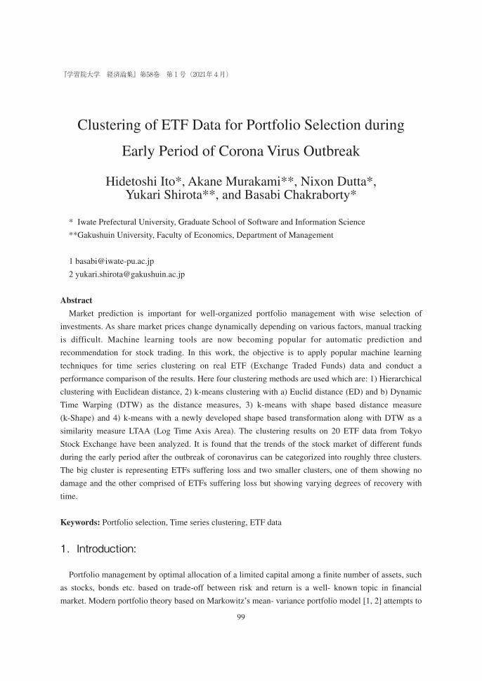
Table 1. ETF data from Tokyo Stock Exchange (Japan).

SerialNumber Name of the ETF Code

Number

1 TOPIX-linked listed investment trusts T1306

2 TOPIX Core 30 Linked Listings T1311

3 Listed Index Fund China A Shares (Panda) T1322

4 UBS ETF Eurozone Large Stock 50 T1385

5 UBS ETF Swiss Shares (MSCI Switzerland) T1391

6 UBS ETF UK Shares (MSCI UK) T1392

7 iShares Core U.S. Treasuries 7-10 E T1482

8 NEXT FUNDS Dow Jones Listed Index T1546

9 Listed Index Fund U.S. Equities (S&P) T1547

10 China H-share bull double-listed investment trust T1572

11 China H-Share Bear Listed Investment Trust T1573

12 TSE Banking Stock Index listed ETF T1615

13 NEXT FUNDS Energy Resources (TOPIX) T1618

14 NEXT FUNDS Construction and Materials(TOPIX) T1619

15 NEXT FUNDS Pharmaceuticals (TOPIX) T1621

16 NEXT FUNDS Iron and Steel, and Non-Ferrous (TOPIX) T1623

17 NEXT FUNDS Electric and Precision Machine (TOPIX) T1625

18 NEXT FUNDS Power and Gas (TOPIX) T1627

19 iShares Core U.S. Treasuries 7-10 E T1656

20 NEXT NOTES Hong Kong Hansen Bear T2032

2.2 Clustering Methods:In this work we have used hierarchical clustering and three similarity measure based partitioning

clustering methods for clustering of ETF data to assess the trend of the stock price movement of different

ETF and to extract the representative pattern of the group of ETF data.

2.2.1 Hierarchical Clustering (HC):Hierarchical clustering is a popular datamining technique in which similar data points are grouped

into a hierarchy of classes in either of the two ways: agglomerative (bottom-up) or divisive (top-down).

Depending on the way of distance measurement between data points within a group and outside of it,

there are several variations of the algorithm. In this work we used single linkage agglomerative HC

algorithm. In the field of portfolio construction, Prado’s proposed HRP (Hierarchical Risk Parity)


103

method has been widely used [3]. One of the main advantage of HRP is an ability in computing a

portfolio on an ill-degenerated or even a singular covariance matrix [4]. After HRP, many researches by

a hierarchical clustering had been conducted [4-7]. We shall conduct the same hierarchical clustering

approach as HRP. Let us explain the method we used.

The input data is the raw data of ETF.

, , (1)

where Si,j represents the i-th ETF’s price on j-th day. The number of ETFs is N and the number of

sales days is T. The size of the matrix , is N times T. From the matrix , , we shall make the

correlation coefficient matrix , , ,…, . In HRP, the distance d is defined as follows:

, , (2)

Then the distance matrix , , ,…, is obtained. Next, selecting any two distance columns,

we shall calculate the Euclid distance as follows:

, ∑ , , (3)

Input the matrix { }, , we shall conduct the hierarchical clustering with single linkage as explained

in the textbook [8]. Then, using the distances between nodes, we shall conduct “quasi-diagonalization”

on the distance matrix { }, .

2.2.2 k-means clustering with Euclid distance (ED) and Dynamic Time Warping(DTW):k- means clustering is the most popular algorithm for partitioning clustering in which data is

partitioned into k groups based on similarity among data points with k prototypes. Euclid distance is the

most common and computationally fastest distance metric and DTW is the most popular metric for

measuring similarity between two different time series. DTW is an elastic measure and work well for

unequal length and shifted time series unlike Euclid distance. The k-means algorithm is dependent on

the value of k (number of clusters) and initial data values of k prototypes. Here we have checked with

different values of k and used the best value according to sum of squared distances from cluster center

(SSD) of the resultant cluster for final clustering of the data set.

2.2.3 k-Shape (k-means with shape based distance measure):k- Shape is a comparatively new time series clustering algorithm developed in [25] for time series

clustering. k-Shape uses a normalized version of cross correlation measure as a distance metric for

comparing similarity of time series based on shape. In [26], authors used k-Shape for analysis of changes

in stock price. We have used here k-Shape for clustering the ETF data.

2.2.4 k-means with Log Time Axis Area(LTAA):Time Axis Area (TAA) is a newly developed shape based transformation technique which can be used

as a similarity measure for time series classification by Ito and Chakraborty in [27]. It is 10 times faster

than DTW in calculating similarity between different time series and is suitable for clustering of time

series. LTAA represents Log Time Axis Area which is the logarithm of TAA. This algorithm actually

104

selects characteristics points from the original time series and use DTW for similarity calculation

between two different time series but as the length of the time series becomes shorter, this technique

takes much shorter time compared to similarity calculation by DTW with the original time series. Here

we used k-means algorithm to cluster the time series with LTAA as the similarity measure.

3. Experimental Results and Analysis:

We will present the results of clustering and their analysis in this section.

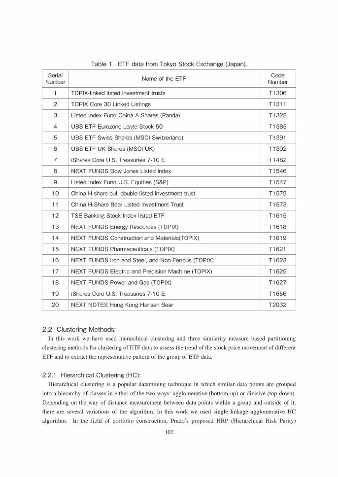
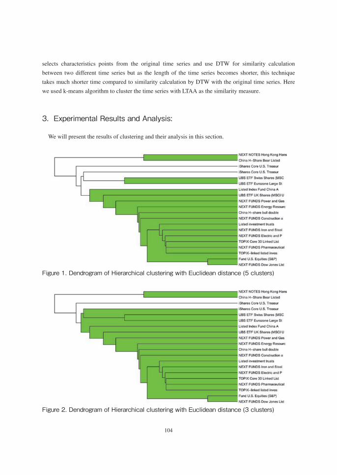
Figure 1. Dendrogram of Hierarchical clustering with Euclidean distance (5 clusters)

of changes in stock price. We have used here k-Shape for clustering the ETF data. 2.2.4 k-means with Log Time Axis Area(LTAA): Time Axis Area (TAA) is a newly developed shape based transformation technique which can be used as a similarity measure for time series classification by Ito and Chakraborty in [27]. It is 10 times faster than DTW in calculating similarity between different time series and is suitable for clustering of time series. LTAA represents Log Time Axis Area which is the logarithm of TAA. This algorithm actually selects characteristics points from the original time series and use DTW for similarity calculation between two different time series but as the length of the time series becomes shorter, this technique takes much shorter time compared to similarity calculation by DTW with the original time series. Here we used k-means algorithm to cluster the time series with LTAA as the similarity measure. 3. Experimental Results and Analysis: We will present the results of clustering and their analysis in this section.

Fig.1 Dendrogram of Hierarchical clustering with Euclidean distance (5 clusters)

Figure 2. Dendrogram of Hierarchical clustering with Euclidean distance (3 clusters)

Fig. 2 Dendrogram of Hierarchical clustering with Euclidean distance (3 clusters) 3.1 Results of Hierarchical Clustering (HC) Fig.1 and Fig. 2 represents the results of clustering by using hierarchical clustering method if we consider 5 clusters and 3 clusters respectively. Fig. 3 shows the correlation co-efficient matrix after quasi diagonalization in which the order of ETF was changed and the greater correlation coefficients are collected diagonally. The Table 2 presents the result of HC. The table represents the clusters of funds (the serial numbers of funds in Table 1 are noted here) considering the different cuts of dendrogram resulting in 2 ,3 and 5 clusters. If we consider 3 clusters, No. 20. Code T2032, No. 11, Code T 1573 are in one cluster, cluster 3 contains only No. 7, Code T1482 which is the US bond ETF with currency exchange hedge, while cluster 2 contains other funds. The third cluster contains only “iShares Core U.S. Treasuries 7-10 E with the hedge” while the other ETF funds falls into the second cluster.


105

3.1 Results of Hierarchical Clustering (HC)Fig.1 and Fig. 2 represents the results of clustering by using hierarchical clustering method if we

consider 5 clusters and 3 clusters respectively. Fig. 3 shows the correlation co-efficient matrix after

quasi diagonalization in which the order of ETF was changed and the greater correlation coefficients are

collected diagonally. The Table 2 presents the result of HC. The table represents the clusters of funds (the

serial numbers of funds in Table 1 are noted here) considering the different cuts of dendrogram resulting

in 2 ,3 and 5 clusters.

If we consider 3 clusters, No. 20. Code T2032, No. 11, Code T 1573 are in one cluster, cluster 3

contains only No. 7, Code T1482 which is the US bond ETF with currency exchange hedge, while

cluster 2 contains other funds. The third cluster contains only “iShares Core U.S. Treasuries 7-10 E with

the hedge” while the other ETF funds falls into the second cluster.

Figure 3. Correlation coefficient matrix after quasi diagonalization

Fig. 3 Correlation coefficient matrix after quasi diagonalization Table 2. Results of Hierarchical Clustering for different cuts of Dendrogram

Number of Clusters

Cluster1 Cluster 2 Cluster 3 Cluster 4 Cluster5

5 11, 20 19 7 4, 5 Other funds 3 11, 20 19, and Other

funds 7 7

2 11, 20 7, 19, 4, 5 and Other funds

3.2 Results of Clustering of k-means with ED and DTW We have experimented with k- means clustering to find the best value of k for both the similarity measures. Fig. 4 represents the MSE (mean square error) of the clusters for different values of k. From the figure it is found that for Euclid distance, k=4 is the best value and for DTW, k=3 represents the correct number of clusters.

Table 2. Results of Hierarchical Clustering for different cuts of DendrogramNumber of Clusters Cluster1 Cluster 2 Cluster 3 Cluster 4 Cluster55 11, 20 19 7 4, 5 Other funds

3 11, 20 19, and Otherfunds 7 7

2 11, 20 7, 19, 4, 5 andOther funds

106

3.2 Results of Clustering of k-means with ED and DTWWe have experimented with k- means clustering to find the best value of k for both the similarity

measures. Fig. 4 represents the MSE (mean square error) of the clusters for different values of k.

From the figure it is found that for Euclid distance, k=4 is the best value and for DTW, k=3 represents

the correct number of clusters.

Figure 4. Sum of squared distance with number of clusters for k-means clustering

Fig 4. Sum of squared distance with number of clusters for k-means clustering Table 3. Clustering results for k-means with ED and DTW

Method Cluster 1 Cluster2 Cluster 3 Cluster 4

k-means(ED) with k=3 (Fig.5)

7,11,19,20 (blue)

1,2,3,4,6,8,9,10,12,13, 14,16,17 (green)

5,15,18 (red)

k-means(ED) with k=4 (Fig. 6)

7,19 (blue)

1,2,3,4,5,6,8,9,10,12, 13,14,16,17 (red)

15,18 (yellow) 11,20 (green)

k-means(DTW) with k=3 (Fig. 7)

7,11,19,20 (green)

1,4,6,12,13.14,16,18 (blue)

2,3,5,8,9,10,15, 17 (red)

k-means(DTW) with k=4 (Fig. 8)

7,11,19,20 (green)

1,12,13,14,16 (blue) 5,8,9,15,18 (red)

2,3,4,6,10, 17 (yellow)

Table 3 presents the clustering results of k-means with ED and DTW for k=3 and k= 4. Fig. 5 and Fig. 6 represent the results of clustering of k-means with ED for k=3 and k=4 in which normalized data is used. It seems from the Table 3 and Fig. 5 that the trend of cluster 1 (blue) shows growth, these group of stocks did not suffer any damage by corona virus outbreak. Cluster 2 (green), the biggest group of stocks suffered the most and could not recover to the original level.

Table 3. Clustering results for k-means with ED and DTW

Method Cluster 1 Cluster2 Cluster 3 Cluster 4

k-means(ED) withk=3 (Fig.5)

7,11,19,20(blue)

1,2,3,4,6,8,9,10,12,13,14,16,17 (green)

5,15,18(red)

k-means(ED) withk=4 (Fig. 6)

7,19(blue)

1,2,3,4,5,6,8,9,10,12,13,14,16,17 (red)

15,18(yellow)

11,20(green)

k-means(DTW)with k=3 (Fig. 7)

7,11,19,20(green)

1,4,6,12,13.14,16,18(blue)

2,3,5,8,9,10,15,17(red)

k-means(DTW)with k=4 (Fig. 8)

7,11,19,20(green)

1,12,13,14,16(blue)

5,8,9,15,18(red)

2,3,4,6,10,17(yellow)

Table 3 presents the clustering results of k-means with ED and DTW for k=3 and k= 4.

Fig. 5 and Fig. 6 represent the results of clustering of k-means with ED for k=3 and k=4 in which

normalized data is used. It seems from the Table 3 and Fig. 5 that the trend of cluster 1 (blue) shows

growth, these group of stocks did not suffer any damage by corona virus outbreak. Cluster 2 (green), the

biggest group of stocks suffered the most and could not recover to the original level.


107

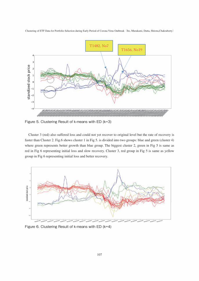
Figure 5. Clustering Result of k-means with ED (k=3)

Fig 5. Clustering Result of k-means with ED (k=3) Cluster 3 (red) also suffered loss and could not yet recover to original level but the rate of recovery is faster than Cluster 2. Fig.6 shows cluster 1 in Fig 5. is divided into two groups: blue and green (cluster 4) where green represents better growth than blue group. The biggest cluster 2, green in Fig 5 is same as red in Fig 6 representing initial loss and slow recovery. Cluster 3, red group in Fig 5 is same as yellow group in Fig 6 representing initial loss and better recovery.

Fig 6. Clustering Result of k-means with ED (k=4)

T1482, No7 T1656, No19

Cluster 3 (red) also suffered loss and could not yet recover to original level but the rate of recovery is

faster than Cluster 2. Fig.6 shows cluster 1 in Fig 5. is divided into two groups: blue and green (cluster 4)

where green represents better growth than blue group. The biggest cluster 2, green in Fig 5 is same as

red in Fig 6 representing initial loss and slow recovery. Cluster 3, red group in Fig 5 is same as yellow

group in Fig 6 representing initial loss and better recovery.

Figure 6. Clustering Result of k-means with ED (k=4)

Fig 5. Clustering Result of k-means with ED (k=3) Cluster 3 (red) also suffered loss and could not yet recover to original level but the rate of recovery is faster than Cluster 2. Fig.6 shows cluster 1 in Fig 5. is divided into two groups: blue and green (cluster 4) where green represents better growth than blue group. The biggest cluster 2, green in Fig 5 is same as red in Fig 6 representing initial loss and slow recovery. Cluster 3, red group in Fig 5 is same as yellow group in Fig 6 representing initial loss and better recovery.

Fig 6. Clustering Result of k-means with ED (k=4)

T1482, No7 T1656, No19

108

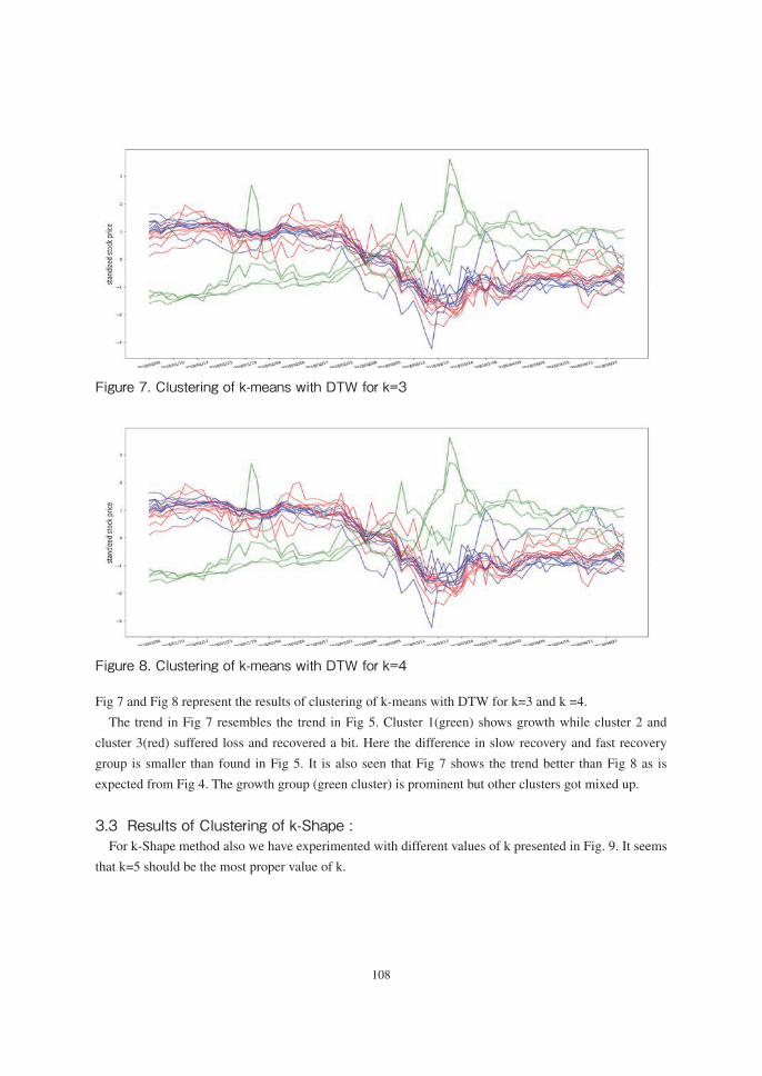
Figure 7. Clustering of k-means with DTW for k=3

Fig. 7 Clustering of k-means with DTW for k=3

Fig. 8 Clustering of k-means with DTW for k=4 Fig 7 and Fig 8 represent the results of clustering of k-means with DTW for k=3 and k =4. The trend in Fig 7 resembles the trend in Fig 5. Cluster 1(green) shows growth while cluster 2 and cluster 3(red) suffered loss and recovered a bit. Here the difference in slow recovery and fast recovery group is smaller than found in Fig 5. It is also seen that Fig 7 shows the trend better than Fig 8 as is expected from Fig 4. The growth group (green cluster) is prominent but other clusters got mixed up.

Figure 8. Clustering of k-means with DTW for k=4

Fig. 7 Clustering of k-means with DTW for k=3

Fig. 8 Clustering of k-means with DTW for k=4 Fig 7 and Fig 8 represent the results of clustering of k-means with DTW for k=3 and k =4. The trend in Fig 7 resembles the trend in Fig 5. Cluster 1(green) shows growth while cluster 2 and cluster 3(red) suffered loss and recovered a bit. Here the difference in slow recovery and fast recovery group is smaller than found in Fig 5. It is also seen that Fig 7 shows the trend better than Fig 8 as is expected from Fig 4. The growth group (green cluster) is prominent but other clusters got mixed up.

Fig 7 and Fig 8 represent the results of clustering of k-means with DTW for k=3 and k =4.

The trend in Fig 7 resembles the trend in Fig 5. Cluster 1(green) shows growth while cluster 2 and

cluster 3(red) suffered loss and recovered a bit. Here the difference in slow recovery and fast recovery

group is smaller than found in Fig 5. It is also seen that Fig 7 shows the trend better than Fig 8 as is

expected from Fig 4. The growth group (green cluster) is prominent but other clusters got mixed up.

3.3 Results of Clustering of k-Shape :For k-Shape method also we have experimented with different values of k presented in Fig. 9. It seems

that k=5 should be the most proper value of k.


109

Figure 9. SSD values for clustering with k-Shape for different values of k

3.3 Results of Clustering of k-Shape : For k-Shape method also we have experimented with different values of k presented in Fig. 9. It seems that k=5 should be the most proper value of k.

Fig 9. SSD values for clustering with k-Shape for different values of k Table 4. Clustering results of k-Shape

Method Cluster1 Cluster2 Cluster3 Cluster4 Cluster5 k-Shape, k=3 (Fig. 10)

3,7,10,13 (red)

2,4,6,11,12,14,16, 19, 20 (green)

1,5,8,9,15,17,18 (blue)

k-Shape, k=5 (Fig. 11)

7,19 (yellow)

1,2,4,8,9,12,14,17 (red)

3,6,10,13,16 (green)

5,15,18 (sky blue)

11,20 (blue)

Fig 10 and Fig 11 represents the results of clustering by k-Shape using shape based distance measure for k=3 and k=5 respectively. The clustering results are shown in Table 4.

Table 4. Clustering results of k-Shape

Method Cluster1 Cluster2 Cluster3 Cluster4 Cluster5


3,7,10,13(red)

2,4,6,11,12,14,16,19, 20 (green)

1,5,8,9,15,17,18(blue)


7,19(yellow)

1,2,4,8,9,12,14,17(red)

3,6,10,13,16(green)

5,15,18(sky blue)

11,20(blue)

Fig 10 and Fig 11 represents the results of clustering by k-Shape using shape based distance measure for

k=3 and k=5 respectively. The clustering results are shown in Table 4.

Figure 10. Clustering Result of k-Shape (k=3)

Fig 10. Clustering Result of k-Shape (k=3)

Fig 11. Clustering Result of k-Shape (k=5) Examining Fig 10 and Fig 11, it is seen that Fig 11 captures the trend of the ETFs grouping better than Fig 10 as is expected from the fact that k=5 is the proper number of k. Now in Fig 11, cluster 1 (yellow) and cluster 5 (blue) represent the group of funds having growth as is found in other methods also. Cluster 2 (red), the largest group, represents the group suffering initial loss and then slow recovery. This also matches with other methods. Cluster 4 (sky blue) represents the group of funds with initial loss and better recovery. Cluster 3 (green) actually resembles cluster 2 with very little difference of larger group variance. They are considered one cluster by other methods.

110

Figure 11. Clustering Result of k-Shape (k=5)

Fig 10. Clustering Result of k-Shape (k=3)

Fig 11. Clustering Result of k-Shape (k=5) Examining Fig 10 and Fig 11, it is seen that Fig 11 captures the trend of the ETFs grouping better than Fig 10 as is expected from the fact that k=5 is the proper number of k. Now in Fig 11, cluster 1 (yellow) and cluster 5 (blue) represent the group of funds having growth as is found in other methods also. Cluster 2 (red), the largest group, represents the group suffering initial loss and then slow recovery. This also matches with other methods. Cluster 4 (sky blue) represents the group of funds with initial loss and better recovery. Cluster 3 (green) actually resembles cluster 2 with very little difference of larger group variance. They are considered one cluster by other methods.

Examining Fig 10 and Fig 11, it is seen that Fig 11 captures the trend of the ETFs grouping better than

Fig 10 as is expected from the fact that k=5 is the proper number of k. Now in Fig 11, cluster 1 (yellow)

and cluster 5 (blue) represent the group of funds having growth as is found in other methods also. Cluster

2 (red), the largest group, represents the group suffering initial loss and then slow recovery. This also

matches with other methods. Cluster 4 (sky blue) represents the group of funds with initial loss and

better recovery. Cluster 3 (green) actually resembles cluster 2 with very little difference of larger group

variance. They are considered one cluster by other methods.

3.4 Results of Clustering of LTAA:Fig. 12 represents the result of LTAA with number of clusters k =3 which seems to be the most

appropriate value for k from experiments with clustering by k-means with LTAA and from other

clustering algorithms used in this study.

Figure 12. Clustering Result of LTAA (k=3)

3.4 Results of Clustering of LTAA: Fig. 12 represents the result of LTAA with number of clusters k =3 which seems to be the most appropriate value for k from experiments with clustering by k-means with LTAA and from other clustering algorithms used in this study.

Fig 12. Clustering Result of LTAA (k=3) Here the three clusters found are as follows: (1) Cluster 1 (red): 7, 19

iShares Core U.S. Treasuries 7-10 E (T 1482) iShares Core U.S. Treasuries 7-10 E (T1656)

This group did not suffer loss due to COVID-19. (2) Cluster 2 (blue): The biggest group (1,2,3,4,5, 6,8,9,10,12,13,14,15,16,17,18)

This group of funds suffer loss and could not recover well. (3) Cluster 3 (green):11, 20 China H-Share Bear Listed Investment Trust (T1573) NEXT NOTES Hong Kong Hansen Bear (T 2032)

This group also relatively low in loss or recovered early. 3.5 Comparative Performance Analysis:

The findings from the different clustering results are summarized in Table 5. It is found from the results of different clustering algorithms that the 20 ETF data can be clustered into three groups for all the clustering algorithms except k-Shape and k-means (ED) for which it is 5 and 4 respectively. This table summarizes the best clusters found from different


111

Here the three clusters found are as follows:

(1)　Cluster 1 (red): 7, 19

　　　・　iShares Core U.S. Treasuries 7-10 E (T 1482)　　　・　iShares Core U.S. Treasuries 7-10 E (T1656)　　This group did not suffer loss due to COVID-19.

(2)　Cluster 2 (blue): The biggest group (1,2,3,4,5, 6,8,9,10,12,13,14,15,16,17,18)

　　This group of funds suffer loss and could not recover well.

(3)　Cluster 3 (green):11, 20

　　　・　China H-Share Bear Listed Investment Trust (T1573)　　　・　NEXT NOTES Hong Kong Hansen Bear (T 2032)　　This group also relatively low in loss or recovered early.

3.5 Comparative Performance Analysis:The findings from the different clustering results are summarized in Table 5. It is found from the

results of different clustering algorithms that the 20 ETF data can be clustered into three groups for all

the clustering algorithms except k-Shape and k-means (ED) for which it is 5 and 4 respectively. This

table summarizes the best clusters found from different algorithms and their respective analysis regarding

the nature of the trend of ETF groups.

Table 5. Summarization of Clustering results of ETF

Method Clusters Comments

HierarchicalClustering (HC)

C1: 11,20C2: 19, othersC3 7

Hong Kong Bear 11 and 20 belong to the same C1

k-means (ED) C1: 7,19, 11,20C2: OthersC3: 5,15,18

US treasuries 7 and 19, and Hong Kong Bear 11 and 20 belong to the same C1

k-means (DTW) C1: 7,11,19,20C2: OthersC3: 2,3,5,8,9,10,15

US treasuries 7 and 19, and Hong Kong Bear 11 and 20 belong to the same C1

k-Shape C1: 7,19C2: othersC3: 3,6,10,13,16C4: 5,15,18C5: 11,20

US treasuries 7 and 19, and Hong Kong Bear 11 and 20 are separated

LTAA C1: 7,19C2: othersC3: 11,20

US treasuries 7 and 19, and Hong Kong Bear 11 and 20 are separated

When we compare the results by k-means (DTW) and by LTAA, we think that LTAA is superior to the

k-means (DTW), because the US treasuries ETFs are separated from the Hong Kong related bear ETFs.

112

The clustering by human beings must be the LTAA result, because the Hong Kong related bear ETFs

have two large peaks.

At least as it concerns the given ETF data, LTAA and k-Shape are superior to the DTW and ED from

the viewpoint that the results by LTAA and k-Shape are more in accordance with human interpretation.

4. Conclusion:

In this work, different machine learning algorithms are used for clustering ETF data obtained during the

early period after corona virus outbreak to analyze the market condition and their performances are

evaluated according to their resemblance with human interpretation. Successful development of effective

machine learning tools for market analysis is supposed to be very much needed in order to develop

automatic techniques for prediction of investment choices. The well-known k-means algorithm for data

clustering with several similarity measures is used here for clustering ETF time series.

We have explored the simplest and low cost Euclid distance and the most effective and computationally

heavy Dynamic Time Warping as the similarity measures. We have also examined two shape based

similarity measures to assess their effectiveness in clustering by k-means algorithm. One of them

k-Shape has been already used in other similar time series clustering problems in financial area. The last

one is LTAA, a newly developed shape based similarity measure used in time series classification.

The experimental results confirm that k-Shape and LTAA have greater potential in clustering ETF data

compared to Euclid distance and DTW as similarity measures for clustering by k-means algorithm. It

can be inferred that as k-Shape and LTAA are based on extracting the shape characteristics of the time

series, they have superior effect in clustering time series of same shape.

References[1] H. Markowitz, "Portfolio Selection," Journal of Finance, pp. 77-91, 1952.

[2] H. Markowitz, "Portfolio selection," Investment under Uncertainty, 1959.

[3] M. L. De Prado, Advances in financial machine learning. John Wiley & Sons, 2018.

[4] R. Clarke, H. De Silva, and S. Thorley, "Portfolio consraints and the fundamental law of active

management," Financial Analysts Journal, vol. 58, no. 5, pp. 48-66, 2002.

[5] M. L. de Prado, "Building diversified portfolios that outperform out of sample," The Journal of

Portfolio Management, vol. 42, no. 4, pp. 59-69, 2016.

[6] M. L. de Prado, Machine Learning for Asset Managers. Cambridge University Press, 2020.

[7] M. Kolanovic and R. T. Krishnamachari, Big Data and AI Strategies. J.P. Morgan, 2017.

[8] T. Raffinot, "Hierarchical clustering-based asset allocation," The Journal of Portfolio anagement,

vol. 44, no. 2, pp. 89-99, 2017.

[9] S. Aghabozorgi, A. S. Shirkhorshidi, and T. Y. Wah, "Time-series clustering–a decade review,"

Information Systems, vol. 53, pp. 16-38, 2015.

[10] S. Chu, E. Keogh, D. Hart, and M. Pazzani, "Iterative deepening dynamic time warping for time


113

series," in Proceedings of the 2002 SIAM International Conference on Data Mining, SIAM, pp.

195-212, 2002.

[11] A. Bagnall and G. Janacek, "Clustering time series with clipped data," Machine Learning, vol. 58,

no. 2-3, pp. 151-178, 2005.

[12] D. J. Berndt and J. Clifford, "Using dynamic time warping to find patterns in time series," in KDD

workshop, vol. 10, no. 16: Seattle, WA, USA:, pp. 359-370, 1994.

[13] X. Xi, E. Keogh, C. Shelton, L. Wei, and C. A. Ratanamahatana, "Fast time series classification

using numerosity reduction," in Proceedings of the 23rd international conference on Machine

learning, pp. 1033-1040, 2006.

[14] Y.-S. Jeong, M. K. Jeong, and O. A. Omitaomu, "Weighted dynamic time warping for time series

classification," Pattern recognition, vol. 44, no. 9, pp. 2231-2240, 2011.

[15] Y.-S. Jeong and R. Jayaraman, "Support vector-based algorithms with weighted dynamic time

warping kernel function for time series classification," Knowledge-based systems, vol. 75, pp. 184-

191, 2015.

[16] H. Y. Sigaki, M. Perc, and H. V. Ribeiro, "Clustering patterns in efficiency and the coming-of-age of

the cryptocurrency market," Scientific reports, vol. 9, no. 1, pp. 1-9, 2019.

[17] P. D’Urso, L. De Giovanni, and R. Massari, "Trimmed fuzzy clustering of financial time series

based on dynamic time warping," Annals of Operations Research, pp. 1-17, 2019.

[18] S. Majumdar and A. K. Laha, "Clustering and classification of time series using topological data

analysis with applications to finance," Expert Systems with Applications, vol. 162, p. 113868, 2020.

[19] P. J. Rousseeuw and L. Kaufman, "Finding groups in data," Hoboken: Wiley Online Library, vol. 1,

1990.

[20] J. MacQueen, "Some methods for classification and analysis of multivariate observations," in

Proceedings of the fifth Berkeley symposium on mathematical statistics and probability, vol. 1, no.

14: Oakland, CA, USA, pp. 281-297, 1967.

[21] M. Massahi, M. Mahootchi, and A. A. Khamseh, "Development of an efficient cluster-based

portfolio optimization model under realistic market conditions," Empirical Economics, pp. 1-20,

2020.

[22] P. E. Puspita, "A Practical Evaluation of Dynamic Time Warping in Financial Time Series

Clustering," in 2020 International Conference on Advanced Computer Science and Information

Systems (ICACSIS), 2020: IEEE, pp. 61-68., 2020

[23] N. Bnouachi r & Abdal lah Mkhadr i (2019) : Effic ien t c lus te r-based por t fo l io

optimization, Communications in Statistics - Simulation and Computation, DOI:

10.1080/03610918.2019.1621341, 2019.

[24] S. Goudarzi, M.J. Jafari and A. Afsar, " A hybrid model for portfolio optimization based on stock

clustering and different investment strategies", International Journal of Economics and Financial Issues, Vol. 7(3), pp. 602-608, 2017.

[25] J. Paparrizos and L. Gravano, "k-Shape: Efficient and Accurate Clustering of Time Series", ACM

SIGMOD Record 45(1):69-76, 2016.

[26] Y. Kishi, T. Hayashi and Y. Ohsawa, “ Analysis of structural changes in domestic stock market”,

114

IEICE Technical Report, Artificial Intelligence and Knowledge-Based Processing, Vol. 118(453),

pp. 57-59, 2019.

[27] H. Ito and B. Chakraborty, “Fast and interpretable transformation for time series classification: A

comparative study”, International Journal of Applied Science and Engineering, Vol 17(3), pp. 269-

280, 2020.

Clustering of ETF Data for Portfolio Selection during ...

Documents

Transcript of Clustering of ETF Data for Portfolio Selection during ...