Clustering, Classification and Explanatory Rules from Harmonic...

4

Clustering, Classification and Explanatory Rules from Harmonic Monitoring Data

Ali Asheibi, David Stirling, Danny Sutanto and Duane Robinson The University of Wollongong

Australia

1. Introduction

With the increased use of power electronics in residential, commercial and industrial distribution systems, combined with the proliferation of highly sensitive micro-processor controlled equipment, a greater number of distribution customers are becoming sensitive to excessive harmonics in the supply system. In industrial systems for example, harmonic losses can increase the operational cost and decrease the useful life of the system equipment (Lamedica, et al., 2001). For these reasons, large industrial and commercial customers are becoming proactive with regards to harmonic monitoring. The deregulation in the utility industry makes it necessary for some utilities to carry out extensive harmonic monitoring programs to retain current customers and targeted new customers by ensuring disturbance levels remain within predetermined limits (Dugan, et al. 2002). This will lead to a rapid escalation of harmonic data that needs to be stored and analysed. Utility engineers are now seeking new tools in order to extract information that may otherwise remain hidden within this large volume of data. Data mining tools are an obvious candidate for assisting in such analysis of large scale data. Data mining can be understood as a process that uses a variety of analysis tools to identify hidden patterns and relationships within data. Classification based on clustering is an important unsupervised learning technique within data mining, in particular for finding a variety of patterns and anomalies in multivariate data through machine learning techniques and statistical methods. Clustering is often used to gain an initial insight into complex data and particularly in this case, to identify underlying classes within harmonic data. Many different types of clustering have been reported in the literature, such as: hierarchical (nested), partitioned (un-nested), exclusive (each object assigned to a cluster), non-exclusive (an object can be assigned to more than one cluster), complete (every object should belong to a cluster), partial (one or more objects belong to none), and fuzzy (an object has a membership weight for all clusters) (Pang, et al., 2006). A method based on the successful AutoClass (Cheeseman & Stutz, 1996) and the Snob research programs (Wallace & Dowe, 1994); (Baxter & Wallace, 1996) has been chosen for our research work on harmonic classification. The method utilizes mixture models (McLachlan, 1992) as a representation of the formulated clusters. This research is principally based on the formation of such mixture models (typically based on Gaussian distributions) through a Minimum Message Length (MML) encoding scheme (Wallace & Boulton, 1968). During the formation of such mixture models the various derivative tools (algorithms) allow O

pen

Acc

ess

Dat

abas

e w

ww

.inte

chw

eb.o

rg

Source: Theory and Novel Applications of Machine Learning, Book edited by: Meng Joo Er and Yi Zhou, ISBN 978-3-902613-55-4, pp. 376, February 2009, I-Tech, Vienna, Austria

www.intechopen.com

Theory and Novel Applications of Machine Learning

46

for the automated selection of the number of clusters and for the calculation of means, variances and relative abundance of the member clusters. In this work a novel technique has been developed using the MML method to determine the optimum number of clusters (or mixture model size) during the clustering process. Once the optimum model size is determined, a supervised learning algorithm is employed to identify the essential features of each member cluster, and to further utilize these in predicting which ideal clusters any new observed data may best described by. This chapter first describes the design and implementation of the harmonic monitoring program and the data obtained. Results from the harmonic monitoring program using both unsupervised and supervised learning techniques are then analyzed and discussed.

2. Harmonic monitoring program

A harmonic monitoring program (Gosbell et al., 2001); (Robinson, 2003) was installed in a typical 33/11kV MV zone substation in Australia that supplies ten 11kV radial feeders. The zone substation is supplied at 33kV from the bulk supply point of a transmission network. Fig. 1 illustrates the layout of the zone substation and feeder system addressed with this harmonic monitoring program. Seven monitors were installed; a monitor at each of the residential, commercial and industrial sites (sites 5-7), a monitor at the sending end of the three individual feeders (sites 2-4) and a monitor at the zone substation incoming supply (Site ID 1). Sites 1-4 in Fig. 1 are all within the substation at the sending end of the feeders identified as being of a predominant load type. Site 5 was along the feeder route approximately 2km from the zone substation, feeds residential area. Site 6 supplies a shopping centre with a number of large supermarkets and many small shops. Site 7 supplies factory manufacturing paper products such as paper towels, toilet paper and tissues. Based on the distribution customer details, it was found that Site 2 comprises 85% residential and 15% commercial, Site 3 comprises 90% commercial and 10% residential and Site 4 comprises 75% industrial, 20% commercial and 5% residential. The monitoring equipment used is the EDMI Mk3 Energy Meter from Electronic Design and Manufacturing Pty. Ltd. (EDMI, 2000). Three phase voltages and currents at sites 1-4 were recorded at the 11kV zone substation and at the 430V sides of the 11kV/430V distribution transformers at sites 5-7, as shown in Fig. 1. The memory capabilities of the above meters, at the time of purchase limited recordings to the fundamental current and voltage in each phase, the current and voltage Total Harmonic Distortion (THD) in each phase, and three other individual harmonics in each phase. For the harmonic monitoring program, the harmonics selected for recording were the 3rd, 5th and 7th harmonic currents and voltages at each monitoring site, since these are typically the most significant harmonics. The memory restrictions of the monitoring equipment dictated that the sampling interval would be constrained to 10 minutes. This follows the suggested measurement time interval by the International Electrotechnical Commission (IEC) standard as given in IEC61000-4-30 for harmonic measurements, inter-harmonic and unbalances waveforms. The standard is regarded as best practice for harmonic measurement and it recommends 10 minute aggregation intervals for routine harmonic survey. Each 10 minute data sample represents the aggregate of the 10-cycle rms (root mean squared) magnitudes over the 10 minutes period. A recent study (Elphick, et al., 2007) suggested that statistically, sampling at faster rate will not provide additional significant extra insight.

www.intechopen.com


47

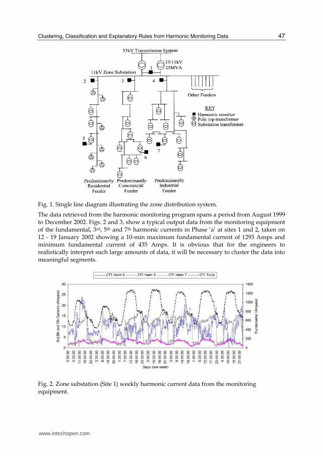
Fig. 1. Single line diagram illustrating the zone distribution system.

The data retrieved from the harmonic monitoring program spans a period from August 1999 to December 2002. Figs. 2 and 3, show a typical output data from the monitoring equipment of the fundamental, 3rd, 5th and 7th harmonic currents in Phase ‘a’ at sites 1 and 2, taken on 12 - 19 January 2002 showing a 10-min maximum fundamental current of 1293 Amps and minimum fundamental current of 435 Amps. It is obvious that for the engineers to realistically interpret such large amounts of data, it will be necessary to cluster the data into meaningful segments.

Fig. 2. Zone substation (Site 1) weekly harmonic current data from the monitoring equipment.

www.intechopen.com


48

3. Minimum Message Length (MML) technique in mixture modelling method

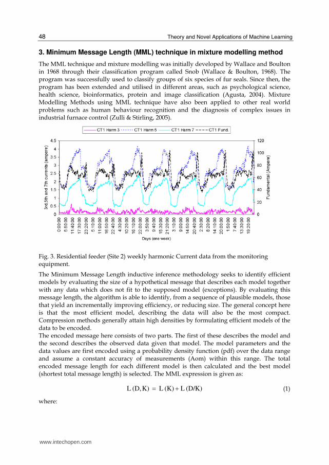
The MML technique and mixture modelling was initially developed by Wallace and Boulton in 1968 through their classification program called Snob (Wallace & Boulton, 1968). The program was successfully used to classify groups of six species of fur seals. Since then, the program has been extended and utilised in different areas, such as psychological science, health science, bioinformatics, protein and image classification (Agusta, 2004). Mixture Modelling Methods using MML technique have also been applied to other real world problems such as human behaviour recognition and the diagnosis of complex issues in industrial furnace control (Zulli & Stirling, 2005).

Fig. 3. Residential feeder (Site 2) weekly harmonic Current data from the monitoring equipment.

The Minimum Message Length inductive inference methodology seeks to identify efficient models by evaluating the size of a hypothetical message that describes each model together with any data which does not fit to the supposed model (exceptions). By evaluating this message length, the algorithm is able to identify, from a sequence of plausible models, those that yield an incrementally improving efficiency, or reducing size. The general concept here is that the most efficient model, describing the data will also be the most compact. Compression methods generally attain high densities by formulating efficient models of the data to be encoded. The encoded message here consists of two parts. The first of these describes the model and the second describes the observed data given that model. The model parameters and the data values are first encoded using a probability density function (pdf) over the data range and assume a constant accuracy of measurements (Aom) within this range. The total encoded message length for each different model is then calculated and the best model (shortest total message length) is selected. The MML expression is given as:

(D/K) L (K) L K)(D, L += (1)

where:

www.intechopen.com


49

K : mixture of clusters in model L (K) : the message length of model K L(D/K) : the message length of the data given the model K L (D, K) : the total message length

Initially given a data set D, the range of measurement and the accuracy of measurement for the data set are assumed to be available. The message length of a mixture of clusters each assuming to have Gaussian distributions with their own mean (µ) and variance (σ) can be calculated as follows: (Oliver & Hand, 1994).

σσ+

μμ=

AOPV

range

AOPV

range

22 loglog (K) L (2)

where:

μrange : range of possible µ values

σrange : range of possible σ values

μAOPV : accuracy of the parameter value of µ

(D/K) L (K) L K)(D, L12

+==μ NsAOPV (3)

s : unbiased sample standard deviation

2

1

)()1(

1xx

Ns

n

ii −∑−= = (4)

N : number of data samples

x : the sample mean

xi : data points AOPVσ: accuracy of the parameter value of σ

1

6

−=σ NsAOPV (5)

The message length of the data using Gaussian distribution model can be calculated from the following equation (Oliver & Hand, 1994):

)(log 2

2log L(D/K) 22

22

2 es

N

ss

NAom

sN

++π= (6)

where: Aom: accuracy of measurement s : sample standard deviation

www.intechopen.com


50

2

1

)(1

xxN

sn

ii −∑= = (7)

An example of how the Mixture Modelling Method using MML technique works, can be illustrated by applying the method to a small data set that contained five distinct distributions of data points (D’s) each of which were randomly generated (D1, D2, …, D5), with its own mean and standard deviation. The generated clusters that were subsequently correctly identified through the MML algorithm are shown in Table 1 and the normal distributions of these clusters are superimposed on the data as shown in Fig. 4.

Table 1. The parameters (μ and σ) of the five generated clusters.

Fig. 4. Five randomly generated clusters each with its own mean and standard deviation.

This mixture modelling approach using the MML technique was used for harmonics classification to discover similar groups of records in the harmonic database; this included clustering the harmonic data from the test system described in section 2. ACPro, a specialised data mining software tool for the automatic segmentation of databases, was primarily used in this work. The preparation of the harmonic data and clustering process are explained in the next section.

3.1 Data preparation and clustering The dominant harmonic currents and voltages attributes identified in Section 2 (3rd, 5th, 7th and THD) were selected from the four different sites; Substation (Site 1), residential (Site 5),

commercial (Site 6) and industrial (Site 7) ⎯ as per Fig. 1. The resulting data set used in this

www.intechopen.com


51

application is one file of 8064 instances which consists of four combined files (4×2016) from the selected sites taken from 12-25 January 2002 inclusive. This data was normalised by dividing each data point by the typical values of each corresponding attribute. The suggested typical value for the harmonic currents is the maximum value whereas for the harmonic voltage is the average value. The maximum value of the harmonic current attributes and the average value of harmonic voltage after normalisation is one. The normalised attributes were selected as input features to the MML algorithm with a given accuracy of measurement (Aom) for each attribute. The number of clusters obtained was automatically determined based on the significance and confidence placed in the measurements, which can be estimated using the entire set of measured data. Each cluster contains a collection of data instances that have been so assembled according to an inferred (learnt) pattern, and the abundance of each group is calculated over the full data range. The abundance value for each cluster represents the proportion of data that is contained in the cluster in relation to the total data set. If for example, only one cluster was formed then the single cluster abundance value will be 100%. Each generated cluster can therefore be considered as a profile of the twelve variables (being the 3rd, 5th, 7th and THD for each of 3 phases) within an acceptable variance. If new data lies beyond the clusters associated variance, another cluster is created. Using a basic spreadsheet tool the clusters are subsequently ordered inversely proportional to the actual abundance, i.e. the most abundant cluster is seen as, s0, and those that are progressively rarer have a high value type numbers.

4. Results and outcomes

The following section provides an array of results and outcomes relating to the mixture modelling afforded by the MML clustering algorithm, as well as other associated techniques. These include the detection of anomalous patterns within the harmonic data and, the simplification or transforming of the mixture model through an abstraction process. Without knowing in advance the appropriate size for a mixture model, i.e. its ideal number of clusters, abstraction to a fewer number of super groups, often assists in perceiving the associated contexts each super group. A range of detail applications illustrates this approach. Subsequent insights arising from these operations have lead to a novel outcome allowing for the prior identification of the correct model size for the harmonic data. Further inspection of interesting clusters or super groups is also facilitated through the use of supervised learning, wherein an essential (or minimal) set of influencing factors behind each is derived in a symbolic form.

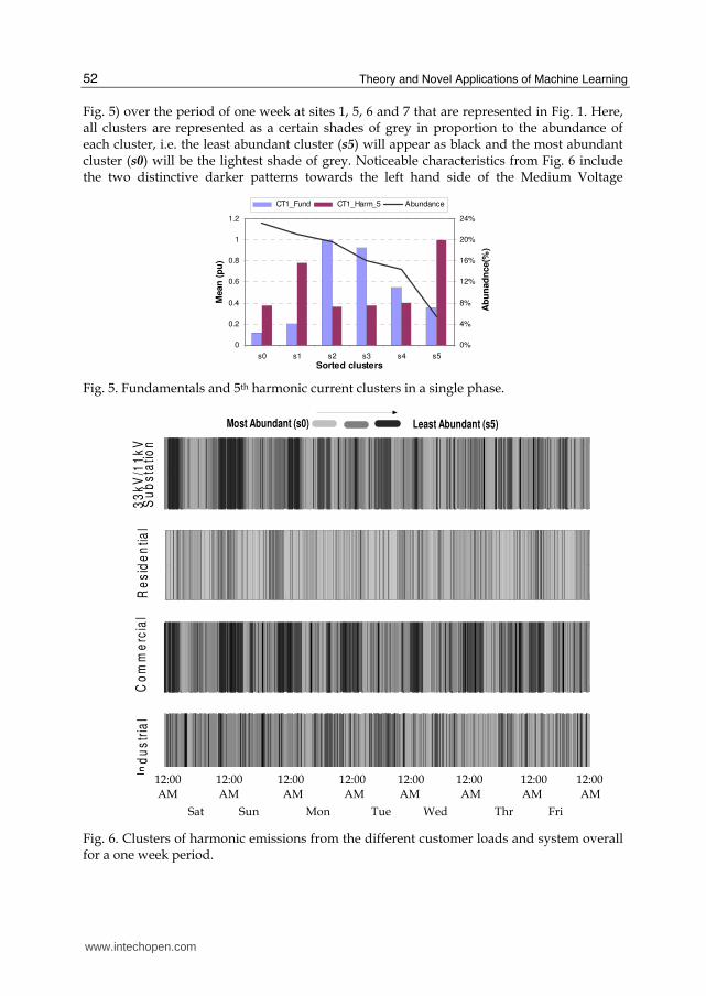
4.1 Anomaly detection and pattern recognition Initially six clusters were specified as input parameters to the MML data mining program, with cluster s5 having the least abundance at 6%. However, the value (mean) of the fifth harmonic in this cluster is at its maximum for all of the data. This cluster (s5) acquires its importance from both the high value of the fifth harmonic current (CT1_Harm_5) and its least number of occurrences. The second highest value of the fifth harmonic current is associated with cluster s1 at 0.78 of the maximum value an abundance of 22%. This cluster might be as important as s5 because it has high fifth harmonic current with a high frequent rate nevertheless the fundamental current (CT1_Fund) is very low. The concept of rare clusters may also be used to identify the most significant distorting loads at different customer sites. Fig. 6 illustrates a mosaic of patterns of the six clusters (see

www.intechopen.com


52

Fig. 5) over the period of one week at sites 1, 5, 6 and 7 that are represented in Fig. 1. Here, all clusters are represented as a certain shades of grey in proportion to the abundance of each cluster, i.e. the least abundant cluster (s5) will appear as black and the most abundant cluster (s0) will be the lightest shade of grey. Noticeable characteristics from Fig. 6 include the two distinctive darker patterns towards the left hand side of the Medium Voltage

0

0.2

0.4

0.6

0.8

1

1.2

s0 s1 s2 s3 s4 s5

Sorted clusters

Mean

(p

u)

0%

4%

8%

12%

16%

20%

24%

Ab

un

ad

nce(%

)

CT1_Fund CT1_Harm_5 Abundance

Fig. 5. Fundamentals and 5th harmonic current clusters in a single phase.

Fig. 6. Clusters of harmonic emissions from the different customer loads and system overall for a one week period.

Su

bs

tatio

nR

es

ide

ntia

lC

om

me

rcia

l

09/04 09/05 09/06 09/07 09/08 09/09 09/10 09/11

Ind

us

tria

l

Most Abundant (s0) Least Abundant (s5)

33

kV

/11

kV

Sat Sun Mon Tue Wed Thr Fri

12:00 12:00 12:00 12:00 12:00 12:00 12:00 12:00 AM AM AM AM AM AM AM AM

www.intechopen.com


53

(MV) 33/11 kV substation data (Site 1). This indicates that the least abundant occurrences

appear during the mornings of the weekend days. Also the commercial site, Site 6, exhibits a

recurring pattern of harmonics over each day, noting that the shopping centre is in

operation seven days a week. The industrial site (site 7) shows that there is a distinctly

different pattern on weekend than during weekdays. The residential customer clusters (site

5) are somewhat more random than the other sites, suggesting that harmonic emission

levels in this site follow no well defined characteristics.

4.2 Abstraction of super groups From the results from the previous section it can be observed that data mining can become a

useful tool for identifying additional information from the harmonic monitoring data,

beyond that which is obtained from standard reporting techniques.

Further additional information can be retrieved by using the Kullback-Lieber (KL) distance

(Duda et al., 2001)which is a measure of similarities and dissimilarities between any two

distributions (clusters). A multidimensional scaling algorithm (MDS) is utilised to process

the resultant KL distances. This enables the generation a 2D geometric visualization

(interpretation) in conjunction with an interactive link analysis, which can ultimately

suggest what combinations of clusters, and neighbourhoods of clusters, could be merged to

form various (fewer) super–groups.

To explain the concept of super−groups, a subset of the harmonic data described in Section 2

being (3rd, 5th, and 7th) from different sites (1, 5, 6, 7) was used as selected attributes for the

MML segmentation. This time ACPro was allowed to determine the number of clusters itself

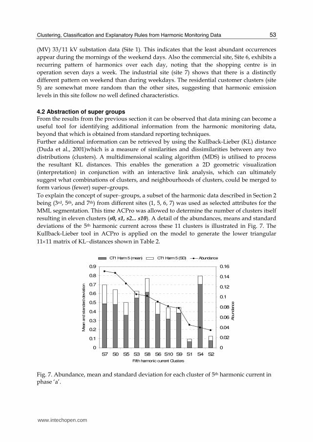
resulting in eleven clusters (s0, s1, s2... s10). A detail of the abundances, means and standard

deviations of the 5th harmonic current across these 11 clusters is illustrated in Fig. 7. The

Kullback-Lieber tool in ACPro is applied on the model to generate the lower triangular

11×11 matrix of KL−distances shown in Table 2.

0

0.1

0.2

0.3

0.4

0.5

0.6

0.7

0.8

0.9

S7 S0 S5 S3 S8 S6 S10 S9 S1 S4 S2

Fifth harmonic current Clusters

Mean a

nd s

tandard

devia

tion

0

0.02

0.04

0.06

0.08

0.1

0.12

0.14

0.16

Abundance

CT1 Harm 5 (mean) CT1 Harm 5 (SD) Abundance

Fig. 7. Abundance, mean and standard deviation for each cluster of 5th harmonic current in phase ‘a’.

www.intechopen.com


54

Table 2. Kullback-Lieber distances between components of the 11 cluster mixture model.

The highlighted distance values represent the three largest and the three smallest distance values. For example, the distance between s3 and s1 is given as 3186, which is the largest distance, which suggests that there is a considerable difference between these two clusters, while on the other hand the distance between s10 and s5 is only 34, which suggests that there is a lot of similarity between these two clusters.

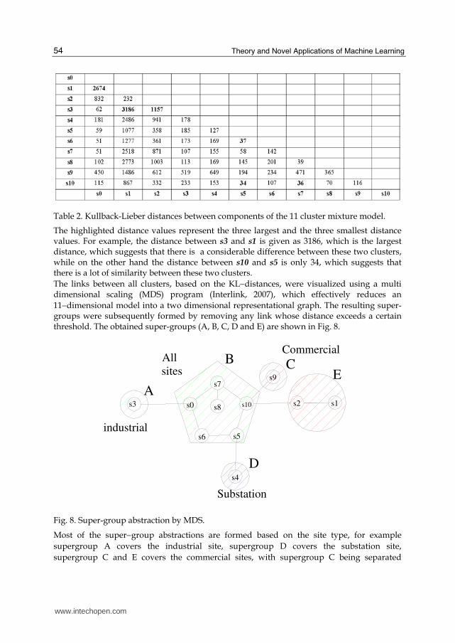
The links between all clusters, based on the KL−distances, were visualized using a multi dimensional scaling (MDS) program (Interlink, 2007), which effectively reduces an

11−dimensional model into a two dimensional representational graph. The resulting super-groups were subsequently formed by removing any link whose distance exceeds a certain threshold. The obtained super-groups (A, B, C, D and E) are shown in Fig. 8.

s3

s7

s8s0 s10

s6 s5

s4

s2 s1

s9

A

B CE

D

industrial

Commercial

Substation

All

sites

Fig. 8. Super-group abstraction by MDS.

Most of the super−group abstractions are formed based on the site type, for example

supergroup A covers the industrial site, supergroup D covers the substation site,

supergroup C and E covers the commercial sites, with supergroup C being separated

www.intechopen.com


55

because the distances between s9 with s2 and s9 with s1 are larger than the distance

between s1 with s2. Super-group B is formed from clusters containing data from all sites.

The residential site does not seem to have a particular supergroup which means that the

influence of harmonic emission (or participation) from this site is very low. The

concurrences of two or more of these super-groups at different sites indicate that there is a

mutual harmonic effect between those sites at that particular time. For example, a temporal

correspondence of super-group A at the industrial site can be observed with both

super−group D at the substation site and super−group E at the commercial site early in the

morning of each day as shown in Fig. 9. The associated pattern of harmonic factors that

might exist in the formation of these super−groups can, in future, be extracted using the

classification techniques of supervised learning.

4.3 Detection of harmonic events The number of the clusters in the previous sections was either specified as input parameters to the MML data mining program or automatically generated by the program itself given a data set D and its accuracy of measurement, Aom. In this section, however, the message length criterion of the MML is utilized to choose the model (number of clusters) that best represent the data. The smaller the encoded message length the better the model fits the data. Therefore the program was controlled to produce a series of models each with an increasing number of clusters for the same fixed values of Aom, and the message lengths of these models have been plotted against the number of clusters as shown in Fig. 10.

12

:00

:00

AM

12

:00

:00

AM

12

:00

:00

AM

12

:00

:00

AM

12

:00

:00

AM

12

:00

:00

AM

12

:00

:00

AM

Time (days)

Commercial SubstationIndustrial Residential

Sat Sun Mon Tue Wed Thu Fri

E

D

C

B

A

Fig. 9. Super-groups in all sites over one week.

In this case, the best model to represent the data was identified as that with six clusters. The

reasoning behind selecting this number of clusters is that the decline in the message length

www.intechopen.com


56

significantly decreases when the model size reaches 6 clusters, and the message length is

comparatively constant afterward as shown in Fig. 10. In other words, this can be

considered to represent the first point of minimum sufficiency for the model.

71000

72000

73000

74000

75000

76000

77000

78000

79000

80000

81000

82000

1 2 3 4 5 6 7 8 9 10 11 12 13 14

Number of clusters

Message length

(B

it)

6 Cluster

Fig. 10. Message length vs. number of generated clusters.

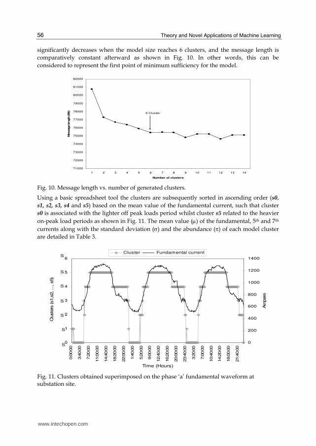
Using a basic spreadsheet tool the clusters are subsequently sorted in ascending order (s0,

s1, s2, s3, s4 and s5) based on the mean value of the fundamental current, such that cluster

s0 is associated with the lighter off peak loads period whilst cluster s5 related to the heavier

on-peak load periods as shown in Fig. 11. The mean value (μ) of the fundamental, 5th and 7th

currents along with the standard deviation (σ) and the abundance (π) of each model cluster

are detailed in Table 3.

0

1

2

3

4

5

6

0:0

0:0

0

3:4

0:0

0

7:2

0:0

0

11:0

0:0

0

14:4

0:0

0

18:2

0:0

0

22:0

0:0

0

1:4

0:0

0

5:2

0:0

0

9:0

0:0

0

12:4

0:0

0

16:2

0:0

0

20:0

0:0

0

23:4

0:0

0

3:2

0:0

0

7:0

0:0

0

10:4

0:0

0

14:2

0:0

0

18:0

0:0

0

21:4

0:0

0

Time (Hours)

Clu

ste

rs (s1,s

2, ..., s

5)

0

200

400

600

800

1000

1200

1400

Am

pere

Cluster Fundamental current

S

S

S

S

S

S

S

Fig. 11. Clusters obtained superimposed on the phase ‘a’ fundamental waveform at substation site.

www.intechopen.com


57

Fundamental current

5th Harmonic current

7th Harmonic current Cluster

Abundance

(π) Mean (μ) SD (σ) Mean (μ) SD (σ) Mean (μ) SD (σ)

s0 0.068386 0.096571 0.041943 0.165865 0.130987 0.062933 0.022882

s1 0.155613 0.106102 0.061533 0.445056 0.123352 0.250804 0.127779

s2 0.056779 0.1694 0.093434 0.300385 0.14996 0.115216 0.028599

s3 0.090994 0.35053 0.132805 0.308374 0.120799 0.330834 0.142327

s4 0.342654 0.38735 0.123757 0.524376 0.193181 0.604311 0.18195

s5 0.285559 0.728608 0.095226 0.5218 0.191722 0.516901 0.149544

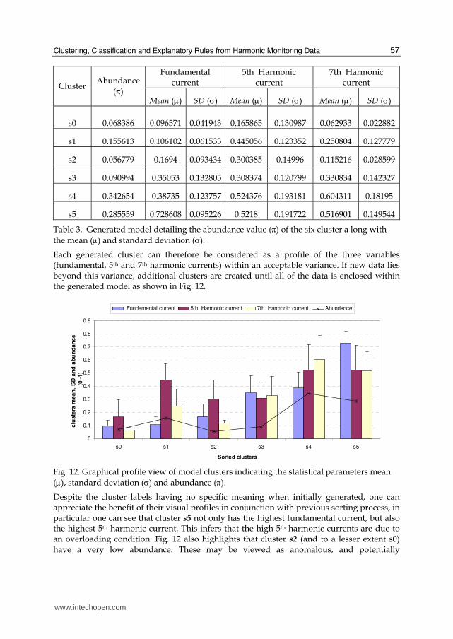
Table 3. Generated model detailing the abundance value (π) of the six cluster a long with

the mean (μ) and standard deviation (σ).

Each generated cluster can therefore be considered as a profile of the three variables (fundamental, 5th and 7th harmonic currents) within an acceptable variance. If new data lies beyond this variance, additional clusters are created until all of the data is enclosed within the generated model as shown in Fig. 12.

0

0.1

0.2

0.3

0.4

0.5

0.6

0.7

0.8

0.9

s0 s1 s2 s3 s4 s5

Sorted clusters

clu

ste

rs m

ea

n,

SD

an

d a

bu

nd

an

ce

(0

-1

)

Fundamental current 5th Harmonic current 7th Harmonic current Abundance

Fig. 12. Graphical profile view of model clusters indicating the statistical parameters mean

(μ), standard deviation (σ) and abundance (π).

Despite the cluster labels having no specific meaning when initially generated, one can appreciate the benefit of their visual profiles in conjunction with previous sorting process, in particular one can see that cluster s5 not only has the highest fundamental current, but also the highest 5th harmonic current. This infers that the high 5th harmonic currents are due to an overloading condition. Fig. 12 also highlights that cluster s2 (and to a lesser extent s0) have a very low abundance. These may be viewed as anomalous, and potentially

www.intechopen.com


58

problematic clusters as described later. Two of these clusters (s5, s2) are further examined to identify different operating conditions based on the various attributes used in the data (fundamental, 5th and 7th harmonic currents) as follows:

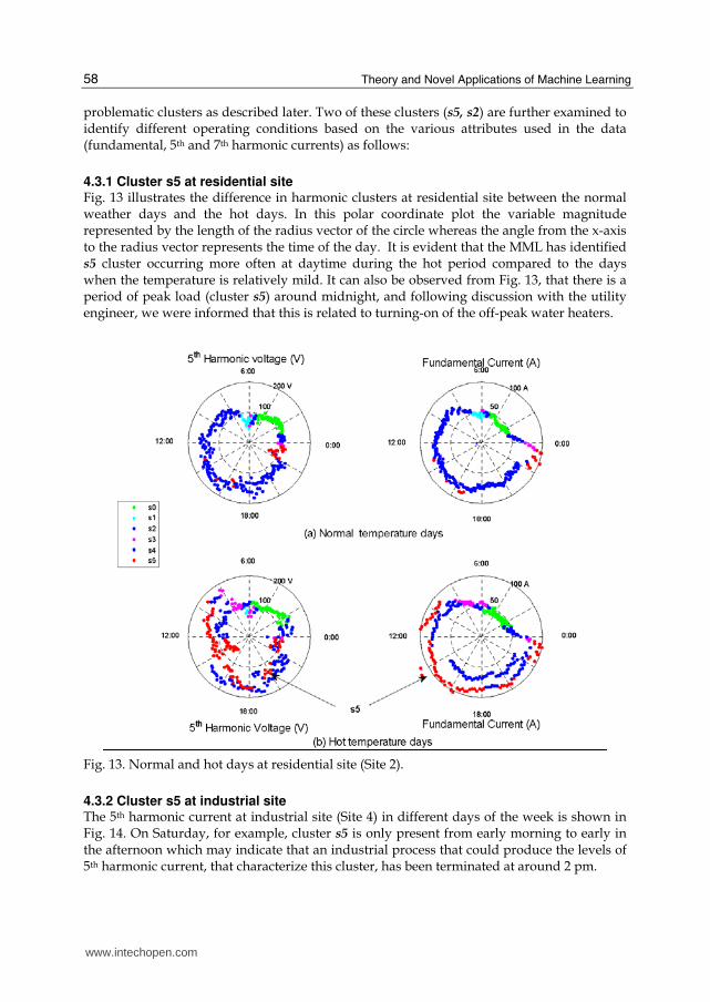
4.3.1 Cluster s5 at residential site Fig. 13 illustrates the difference in harmonic clusters at residential site between the normal weather days and the hot days. In this polar coordinate plot the variable magnitude represented by the length of the radius vector of the circle whereas the angle from the x-axis to the radius vector represents the time of the day. It is evident that the MML has identified s5 cluster occurring more often at daytime during the hot period compared to the days when the temperature is relatively mild. It can also be observed from Fig. 13, that there is a period of peak load (cluster s5) around midnight, and following discussion with the utility engineer, we were informed that this is related to turning-on of the off-peak water heaters.

Fig. 13. Normal and hot days at residential site (Site 2).

4.3.2 Cluster s5 at industrial site The 5th harmonic current at industrial site (Site 4) in different days of the week is shown in Fig. 14. On Saturday, for example, cluster s5 is only present from early morning to early in the afternoon which may indicate that an industrial process that could produce the levels of 5th harmonic current, that characterize this cluster, has been terminated at around 2 pm.

www.intechopen.com


59

Fig. 14. 5th harmonic current clusters at industrial site for different week days.

On Sunday however, the cluster s5 has disappeared inferring that these loads were off. These loads were on again during the weekday at day and night time showing the long working hours in this small factory at the weekdays. Similar results of the 5th harmonic current can be seen at the commercial site, see Fig. 15.

Fig. 15. 5th harmonic current clusters at commercial site for two different week days.

4.3.3 Cluster s2 at substation site. Generally by examining the behaviour of MML model classifications (based on the recorded data) one is able to attribute further meaning to each of its cluster components(Asheibi, 2006). For example, it is noted that there are several sudden changes to cluster s2 at particular time instances during the day. It appears from Fig. 16(b) that this is due to sudden changes in the 7th harmonic current. After further investigation of the reactive power (MVAr) measurement at the 33kV side of the power system shown in Fig. 16(c), it can be deduced that the second cluster (s2) is related to a capacitor switching event. Early in the morning, when the system MVAr demand is high as shown in Fig. 16(c), the capacitor is switched on in the 33kV side to reduce bus voltage and late at night when the system MVAr demand is low, the capacitor is switched off to avoid excessive voltage rise. By just observing the fundamental current, it is

www.intechopen.com


60

difficult to understand why the second cluster has been generated. The 7th harmonic current and voltage plots as shown in Fig. 16(b) provides a clue that something is happening during cluster s2, in that the 7th harmonic current increases rapidly and 7th harmonic voltage decreases, although the reason is still unknown. In this case, the clustering process correctly identified this period as a separate cluster compared to other events, and this can be used to alert the power system operator of the need to understand the reasoning for the generation of such a cluster, particularly when considering the fact that the abundance value for s2 is quite low (5%). When contacted, the operator identified this period as a capacitor switching event which can be verified from the MVAr plot of the system (which was not used in the clustering algorithm). The capacitor switching operation in the 33kV side can also be detected at the other sites (sites 2, 3 and 4) at the 11kV side.

0:00 6:00 12:00 18:00 0:00 6:00 12:00 18:00 0:00-10

0

10

20

Time (Hours)

Reactive p

ow

er

(MV

A r

)

0

500

1000

1500

Fundam

enta

l curr

ent

(A)

0

1

2

3

4

5

6

0

1

2

3

4

5

6

(a)

(c)

Clu

ste

r

0

5

10

15

20

7 t h

Harm

onic

curr

ent

(A)

0

20

40

60

80

0

20

40

60

80

(b)7 t h

Harm

onic

voltage (

V)

I 1

Cap On

Cap Off

V 7

I 7

Fig. 16. Clusters at substation site in two working days (a) Clusters superimposed on the fundamental current waveform, (b) 7th harmonic current and voltage data. (c) MVAr load at the 33kV.

4.4 Determination of the optimum number of clusters in harmonic data Determining the optimum number of clusters becomes important since overestimating the

number of clusters will produce a large number of clusters each of which may not

necessarily represent truly unique operating conditions, whereas underestimation leads to

only small number of clusters each of which may represent a combination of specific events.

A method is developed to determine the optimum number of clusters, each of which

represents a unique operating condition. The method is based on the trend of the

exponential difference in message length when using the MML algorithm. The MML states

www.intechopen.com


61

that the best theory or model K is the one that produces the shortest message length of that

model and data D given that model. From information theory, minimizing the message

length in an MML technique is equivalent to maximizing the posterior probability in

Bayesian theory (Oliver, et al. , 1996). This posterior probability of Bayes’ theorem is given

by:

Prob(D)

(D/K) L * (K) Prob K)|(D Prob = (8)

Since the minimum message length in (1), is equivalent to the maximum posterior

probability in (8), this yields:

)|(Pr)|( KDobKDL = (9)

This suggests that the message length declines as more clusters are generated and hence the difference between the message lengths of two consecutive mixture models is close to zero as it approaches its optimum value and stays close to zero. A series of very small values of the difference of the message length of two consecutive mixture models can then be used as an indicator that an optimum number of clusters has been found. Further, this difference can be emphasised by calculating the exponential of the change in message length for consecutive mixture models, which in essence represents the probability of the model correctness prob(D|K). If this value remains constant at around 1 for a series of consecutive mixture models then the first time it reaches this value can be considered to be the optimum number of clusters. To illustrate the use of the exponential message length difference curve on determining the optimal number of clusters for the harmonic monitoring system described in Section 2, the measured fundamental, 5th and 7th harmonic currents from sites 1, 2, 3 and 4 in Fig.1 (taken on 12 -19 January 2002) were used as the input attributes to the MML algorithm (here ACPro). The trend in the exponential message length difference for consecutive pairs of mixture models is shown in Fig. 17. Here, the exponential of the message length difference does not remain at 1 after it initially approaches it, but rather oscillates close to 1. This is because the algorithm applies various heuristics in order to avoid any local minima that may prevent it from further improving the message length. Once the algorithm appears to be trapped at the local minima, ACPro tries to split, merge, reclassify and swap the data in the clusters found so far to determine if by doing so it may result in a better (lower) message length. This leads to sudden changes to the message length and more often than not, the software can generate large number of clusters which are generally not optimum. This results in the exponential, message length difference deviating away from 1 to a lower

value, after which it gradually returns back to 1. To cater for this, the optimum number of

clusters is chosen when the exponential difference in message length first reaches its highest

value. Using this method, it can be concluded that the optimum number of cluster is 16,

because this is the first time it reaches its highest value close to 1 at 0.9779. With the help of

the operation engineers, the sixteen clusters detected by this exponential method were

interpreted as given in Table 4. It is virtually impossible to obtain these 16 unique events by

visual observation of the waveforms shown in Fig. 18.

www.intechopen.com


62

0 5 10 15 20 25

10-4

10-2

100

0 5 10 15 20 25

10-0.3

100

100.3

Model of consecutive clusters

Ex

po

ne

nti

al

of

me

ss

ag

e d

iffe

ren

ce

16 clusters

Fig. 17. Exponential curve detect sixteen clusters of harmonic data.

Cluster Event

s0 5th harmonic loads at Substation due to Industrial site

s1 Off peak load at Substation site

s2 Off peak load at Commercial site

s3 Off peak at load Commercial due to Industrial

s4 Off peak at Industrial site

s5 Off peak at Substation site

s6 and s7 Switching on and off of capacitor at Substation site

s8 Ramping load at industrial site

s9 Switch on harmonic load at Industrial

s10 Ramping load at Residential site

s11 Ramping load at Commercial site

s12 Switching on TV’s at Residential site

s13 Switching on harmonic loads at Industrial and Residential

s14 Ramping load at Substation due to Commercial

s15 On peak load at Substation due to Commercial

Table 4. The 16 clusters by the method of exponential difference in message length.

www.intechopen.com


63

4.5 Classification of the optimal number of clusters in harmonic data The C5.0 algorithm classification tool was applied to the measured data set and the sixteen

generated clusters, obtained from the previous section, as class labels to this data. The C5.0

algorithm is an advanced supervised learning tool with many features that can efficiently

induce plausible decision trees and also facilitate the pruning process. The resulting models

can either be represented as tree-like structures, or as rule sets, both of which are symbolic

and can be easily interpreted. The usefulness of decision trees, unlike neural networks, is

that it performs classification without requiring significant training, and its ability to

generate a visualized tree, or subsequently expressible and understandable rules.

Fig. 18. Sixteen clusters superimposed on four sites (a) Substation, (b) Residential, (c) Commercial and (d) Industrial.

Two main problems may arise when applying the C5.0 algorithm on continuous attributes

with discrete symbolic output classes. Firstly, the resulting decision tree may often be very

large for humans to easily comprehend as a whole. The solution to this problem is to

transform the class attribute, of several possible alternative values, into a binary set

including the class to be characterised as first class and all other classes combined as the

second class. Secondly, too many rules might be generated as a result of classifying each

data point in the training data set to belong to which recognized cluster. To overcome this

problem, the data is split into ranges instead of continuous data. These ranges can be built

from the average parameters (mean (μ), standard deviation (σ)) of data distributions as

listed in Table 5 and visualised in Fig. 19.

www.intechopen.com


64

Range Range Name

[ 0 , μ–2*σ ] Very Low (VL)

[ μ–2*σ , μ–σ ] Low (L)

[ μ–σ , μ+σ ] Medium (M)

[ μ+σ , μ+2*σ ] High (H)

[ μ+2*σ , 1 ] Very High (VH)

Table 5. The continuous data is grouped into five ranges.

.2 .3 .4 .5 .6 .7 .8 .9

Fig. 19. The five regions of Gaussian distribution used to convert the numeric values.

4.6 Rules discovered from the optimum clusters using decision tree Using the symbolic values (VL, L, M, H and VH) of input attributes (fundamental, 5th and

7th harmonic current) and the binary sets of classes {(s0, other), (s1, other)…. (s15, other)}

the C5.0 algorithm has been applied to as much times as the number of clusters (16 times)

to uncover and define the minimal expressible and understandable rules behind each of

the harmonic-level contexts associated with each of the sixteen cluster described in

Section 4.4. Samples of these rules is shown in Table 6 for both s12 which has been

identified as the cluster associated with switching on TV’s at the residential site and s13

which is a cluster encompassing the engagement of other harmonic loads at both

industrial and residential sites. The quality measure of each rule is described by two

numbers (m, n) shown in Table 6, in brackets, preceding the description of each rules,

where:

m: the number of instances assigned to the rule and

n: the proportion of correctly classified instances.

Very Low

Low

Medium

High

Very High

Normal (0.56951, 0.12993)

www.intechopen.com


65

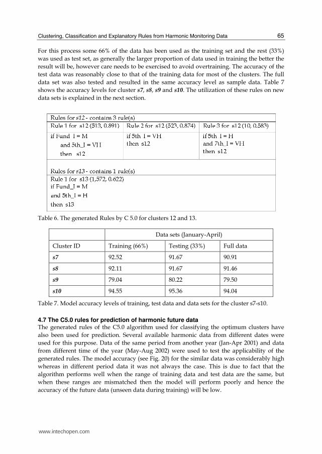
For this process some 66% of the data has been used as the training set and the rest (33%)

was used as test set, as generally the larger proportion of data used in training the better the

result will be, however care needs to be exercised to avoid overtraining. The accuracy of the

test data was reasonably close to that of the training data for most of the clusters. The full

data set was also tested and resulted in the same accuracy level as sample data. Table 7

shows the accuracy levels for cluster s7, s8, s9 and s10. The utilization of these rules on new

data sets is explained in the next section.

Table 6. The generated Rules by C 5.0 for clusters 12 and 13.

Data sets (January-April)

Cluster ID Training (66%) Testing (33%) Full data

s7 92.52 91.67 90.91

s8 92.11 91.67 91.46

s9 79.04 80.22 79.50

s10 94.55 95.36 94.04

Table 7. Model accuracy levels of training, test data and data sets for the cluster s7-s10.

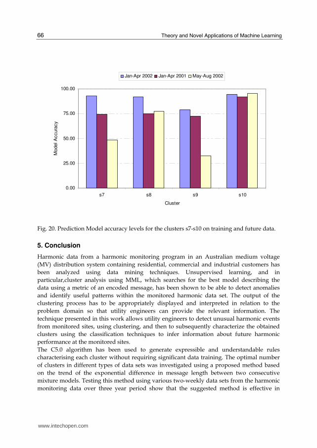
4.7 The C5.0 rules for prediction of harmonic future data The generated rules of the C5.0 algorithm used for classifying the optimum clusters have

also been used for prediction. Several available harmonic data from different dates were

used for this purpose. Data of the same period from another year (Jan-Apr 2001) and data

from different time of the year (May-Aug 2002) were used to test the applicability of the

generated rules. The model accuracy (see Fig. 20) for the similar data was considerably high

whereas in different period data it was not always the case. This is due to fact that the

algorithm performs well when the range of training data and test data are the same, but

when these ranges are mismatched then the model will perform poorly and hence the

accuracy of the future data (unseen data during training) will be low.

www.intechopen.com


66

0.00

25.00

50.00

75.00

100.00

s7 s8 s9 s10

Cluster

Model A

ccura

cy

Jan-Apr 2002 Jan-Apr 2001 May-Aug 2002

Fig. 20. Prediction Model accuracy levels for the clusters s7-s10 on training and future data.

5. Conclusion

Harmonic data from a harmonic monitoring program in an Australian medium voltage

(MV) distribution system containing residential, commercial and industrial customers has

been analyzed using data mining techniques. Unsupervised learning, and in

particular,cluster analysis using MML, which searches for the best model describing the

data using a metric of an encoded message, has been shown to be able to detect anomalies

and identify useful patterns within the monitored harmonic data set. The output of the

clustering process has to be appropriately displayed and interpreted in relation to the

problem domain so that utility engineers can provide the relevant information. The

technique presented in this work allows utility engineers to detect unusual harmonic events

from monitored sites, using clustering, and then to subsequently characterize the obtained

clusters using the classification techniques to infer information about future harmonic

performance at the monitored sites.

The C5.0 algorithm has been used to generate expressible and understandable rules

characterising each cluster without requiring significant data training. The optimal number

of clusters in different types of data sets was investigated using a proposed method based

on the trend of the exponential difference in message length between two consecutive

mixture models. Testing this method using various two-weekly data sets from the harmonic

monitoring data over three year period show that the suggested method is effective in

www.intechopen.com


67

determining the optimum number of clusters in harmonic monitoring data. The continuous

data has been split into ranges to avoid too many rules that might be generated. The C5.0

algorithms were then used to generate considerable number of rules for classification and

prediction of the optimum clusters.

6. References

Agusta, Y. (2004). Minimum Message Length Mixture Modelling for Uncorrelated and Correlated Continuous Data Applied to Mutual Funds Classification, PhD Thesis, Monash University, Clayton, Victoria, Australia.

Asheibi, A., Stirling, D. and Soetanto, D. (2006). Analyzing Harmonic Monitoring Data Using Data Mining. In Proc. Fifth Australasian Data Mining Conference (AusDM2006), Sydney, Australia. CRPIT, 61. Peter, C., Kennedy, P.J., Li, J., Simoff, S.J. and Williams, G.J., Eds., ACS. 63-68.

Cheeseman, P.; Stutz, J. (1996). Bayesian Classification (AUTOCLASS): Theory and Results, In Advances in Knowledge Discovery and Data Mining, Fayyad, U.; Piatetsky-Shapiro, G.; Smyth, P.; Uthurusanny, R., eds, pp. 153-180, AAAI press, Menlo Park, California.

Elphick, S.; Gosbell, V. & Perera, S. (2007). The Effect of Data Aggregation Interval on Voltage Results, Proceedings of Australasian Universities Power Engineering Conference AUPEC07, Dec. 2007, Perth, Australia, Paper 15-02

Gosbell, V.; Mannix, D.; Robinson, D. ; Perera, S. (2001) Harmonic Survey of an MV distribution system, Proceedings of Australasian Universities Power Engineering Conference, pp. 338-342, 23-26 September 2001, Perth, Australia.

Interlink, Knowledge Network Organising Tool (2007), KNOT, 24 August, 2007. http://www.interlinkinc.net/KNOT.html,

Lamedica, R.; Esposito, G.; Tironi, E.; Zaninelli, D. & Prudenzi, A. (2001) A survey on power quality cost in industrial customers. Proceedings of IEEE PES Winter Meeting, Vol 2, pp. 938 – 943.

McLachlan, G. (1992). Discriminant Analysis and Statistical Pattern Recognition, Wiley, New York.

Oliver, J.; Baxter, R. & Wallace, C. (1996). Unsupervised Learning using MML, Proceedings of the 13th Int. Conf in Machine Learning:( ICML-96), pp. 364-372.

Oliver, J. J. & Hand, D. J. (1994) Introduction to Minimum Encoding Inference, [TR 4-94] Dept. Statistics. Open University. Walton Hall, Milton Keynes,UK.

Pang, T.; Steinbach, M. & Kumar V. (2006). Introduction to Data Mining, Pearson Education, Boston.

Robinson, D., “Harmonic Management in MV Distribution System” PhD Thesis, University of Wollongong, 2003.

Wallace, C.; Boulton D.M. (1968). An information measure for classification The Computer Journal, Vol 11, No 2, August 1968, pp185-194.

Wallace, C.; Dowe D. (1994). Intrinsic classification by MML – the Snob program, proceeding of 7th Australian Joint Conf. on Artificial Intelligence, World Scientific Publishing Co., Armidale, Australia,1994.

Wallace, C. (1998). Intrinsic Classification of Spatially Correlated Data, The Computer Journal, Vol. 41, No. 8.

www.intechopen.com


68

Zulli, P.; Stirling, D. (2005) "Data Mining Applied to Identifying Factors Affecting Blast Furnace Stave Heat Loads," Proceedings of the 5th European Coke and Ironmaking Congress.

www.intechopen.com

Theory and Novel Applications of Machine LearningEdited by Meng Joo Er and Yi Zhou

ISBN 978-953-7619-55-4Hard cover, 376 pagesPublisher InTechPublished online 01, January, 2009Published in print edition January, 2009

InTech EuropeUniversity Campus STeP Ri Slavka Krautzeka 83/A 51000 Rijeka, Croatia Phone: +385 (51) 770 447 Fax: +385 (51) 686 166www.intechopen.com

InTech ChinaUnit 405, Office Block, Hotel Equatorial Shanghai No.65, Yan An Road (West), Shanghai, 200040, China

Phone: +86-21-62489820 Fax: +86-21-62489821

Even since computers were invented, many researchers have been trying to understand how human beingslearn and many interesting paradigms and approaches towards emulating human learning abilities have beenproposed. The ability of learning is one of the central features of human intelligence, which makes it animportant ingredient in both traditional Artificial Intelligence (AI) and emerging Cognitive Science. MachineLearning (ML) draws upon ideas from a diverse set of disciplines, including AI, Probability and Statistics,Computational Complexity, Information Theory, Psychology and Neurobiology, Control Theory and Philosophy.ML involves broad topics including Fuzzy Logic, Neural Networks (NNs), Evolutionary Algorithms (EAs),Probability and Statistics, Decision Trees, etc. Real-world applications of ML are widespread such as PatternRecognition, Data Mining, Gaming, Bio-science, Telecommunications, Control and Robotics applications. Thisbooks reports the latest developments and futuristic trends in ML.

How to referenceIn order to correctly reference this scholarly work, feel free to copy and paste the following:

Ali Asheibi, David Stirling, Danny Sutanto and Duane Robinson (2009). Clustering, Classification andExplanatory Rules from Harmonic Monitoring Data, Theory and Novel Applications of Machine Learning, MengJoo Er and Yi Zhou (Ed.), ISBN: 978-953-7619-55-4, InTech, Available from:http://www.intechopen.com/books/theory_and_novel_applications_of_machine_learning/clustering__classification_and_explanatory_rules__from_harmonic_monitoring_data

© 2009 The Author(s). Licensee IntechOpen. This chapter is distributedunder the terms of the Creative Commons Attribution-NonCommercial-ShareAlike-3.0 License, which permits use, distribution and reproduction fornon-commercial purposes, provided the original is properly cited andderivative works building on this content are distributed under the samelicense.

https://creativecommons.org/licenses/by-nc-sa/3.0/

Clustering, Classification and Explanatory Rules from Harmonic...

Documents

Transcript of Clustering, Classification and Explanatory Rules from Harmonic...