Cluster analysis

Jens C. FrisvadBioCentrum-DTU

Biological data analysis and chemometrics

Based on H.C. Romesburg: Cluster analysis for researchers,Lifetime Learning Publications, Belmont, CA, 1984P.H.A. Sneath and R.R. Sokal: Numericxal Taxonomy, Freeman, San Fransisco, CA, 1973

Two primary methods

• Cluster analysis (no projection)– Hierarchical clustering– Divisive clustering– Fuzzy clustering

• Ordination (projection)– Principal component analysis– Correspondence analysis– Multidimensional scaling

Advantages of cluster analysis

• Good for a quick overview of data• Good if there are many groups in data• Good if unusual similarity measures are

needed• Can be added on ordination plots (often as a

minimum spanning tree, however)• Good for the nearest neighbours, ordination

better for the deeper relationships

Different clustering methods• NCLAS: Agglomerative clustering by distance

optimization• HMCL: Agglomerative clustering by homogeneity

optimization• INFCL: Agglomerative clustering by information theory

criteria• MINGFC: Agglomerative clustering by global

optimization• ASSIN: Divisive monothetic clustering• PARREL: Partitioning by global optimization• FCM: Fuzzy c-means clustering• MINSPAN: Minimum spanning tree• REBLOCK: Block clustering (k-means clustering)

SAHN clustering

• Sequential agglomerative hierarchicnonoverlapping clustering

Single linkage

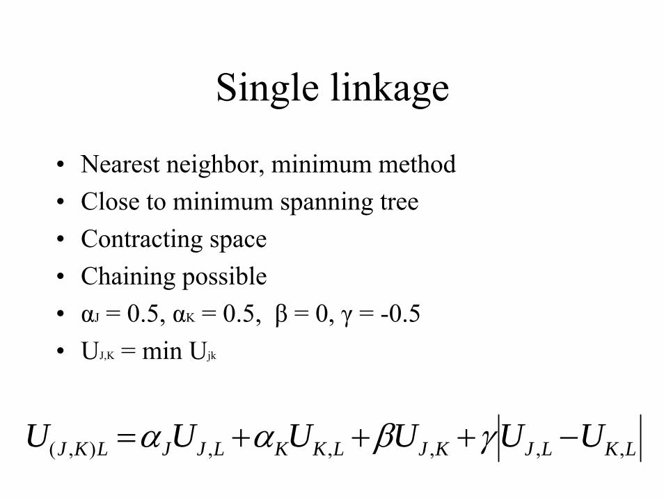
• Nearest neighbor, minimum method• Close to minimum spanning tree• Contracting space• Chaining possible• αJ = 0.5, αK = 0.5, β = 0, γ = -0.5• UJ,K = min Ujk

LKLJKJLKKLJJLKJ UUUUUU ,,,,,),( −+++= γβαα

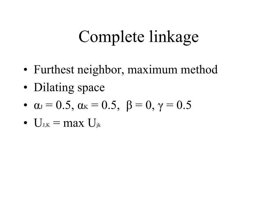
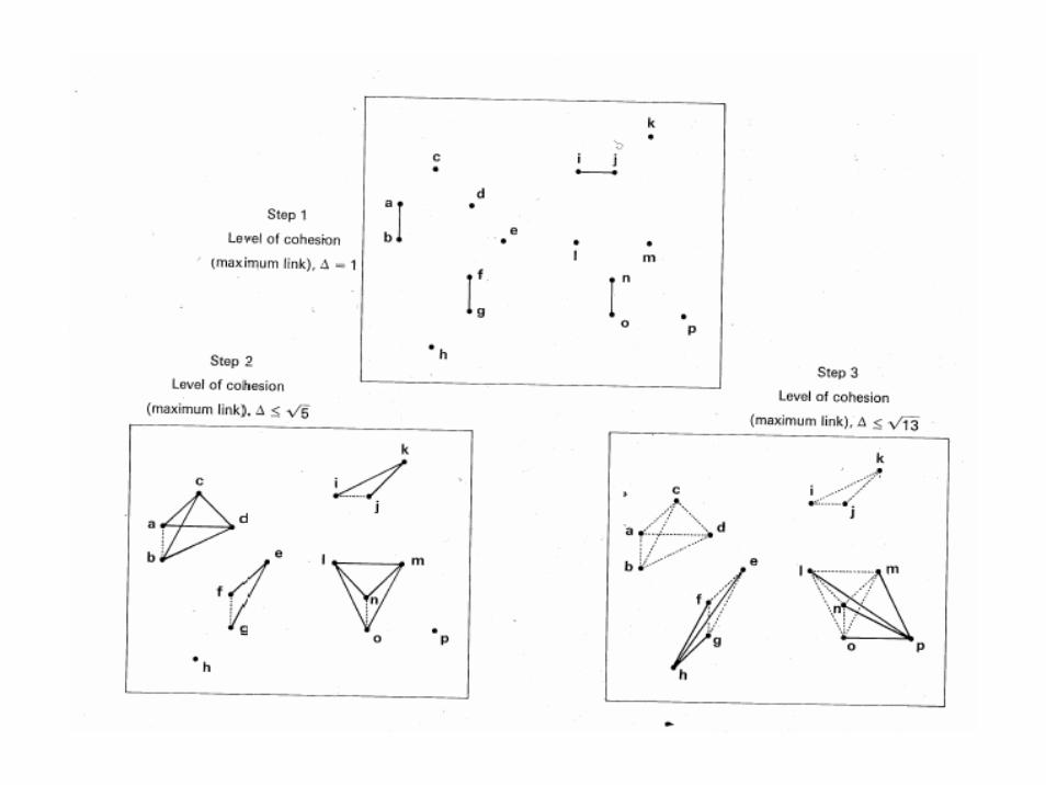
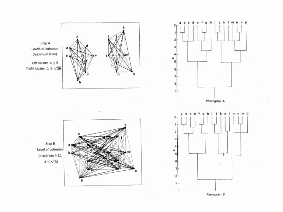
Complete linkage

• Furthest neighbor, maximum method• Dilating space• αJ = 0.5, αK = 0.5, β = 0, γ = 0.5• UJ,K = max Ujk

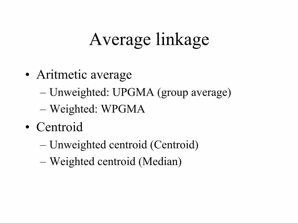
Average linkage

• Aritmetic average– Unweighted: UPGMA (group average)– Weighted: WPGMA

• Centroid– Unweighted centroid (Centroid)– Weighted centroid (Median)

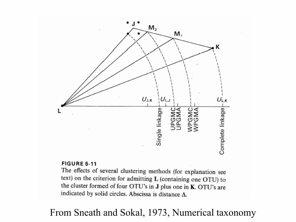
From Sneath and Sokal, 1973, Numerical taxonomy

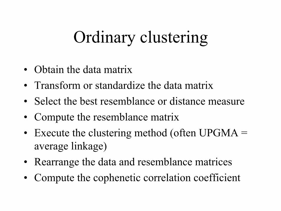
Ordinary clustering

• Obtain the data matrix• Transform or standardize the data matrix• Select the best resemblance or distance measure• Compute the resemblance matrix• Execute the clustering method (often UPGMA =

average linkage)• Rearrange the data and resemblance matrices• Compute the cophenetic correlation coefficient

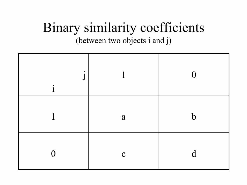
Binary similarity coefficients(between two objects i and j)

ji

1 0

1 a b

0 c d

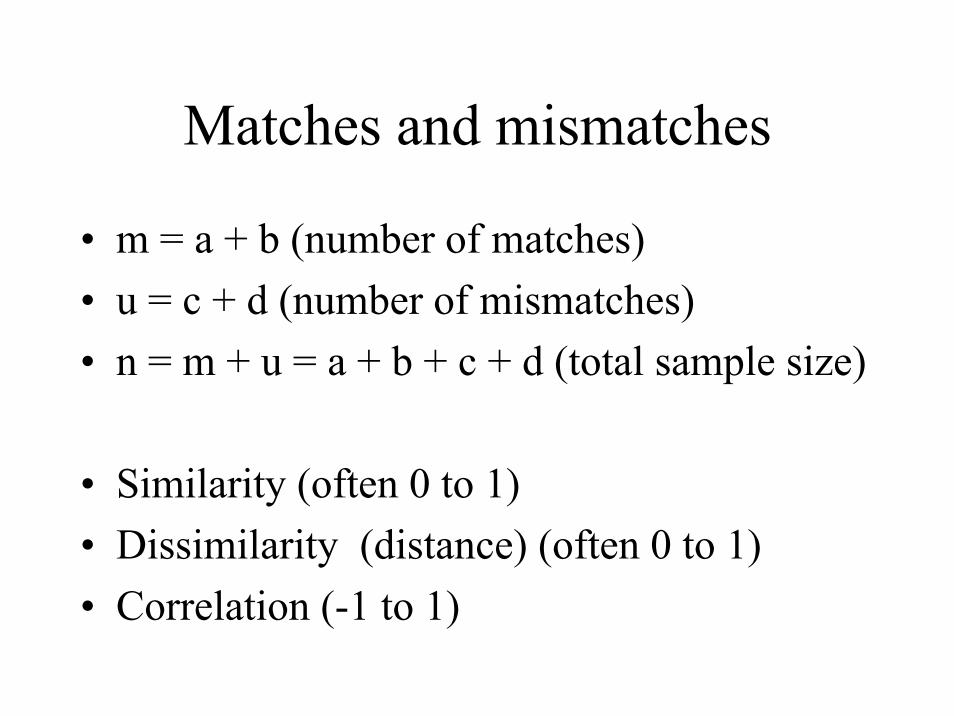
Matches and mismatches

• m = a + b (number of matches)• u = c + d (number of mismatches)• n = m + u = a + b + c + d (total sample size)

• Similarity (often 0 to 1)• Dissimilarity (distance) (often 0 to 1)• Correlation (-1 to 1)

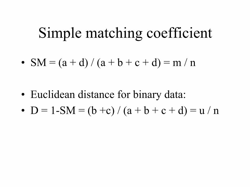
Simple matching coefficient

• SM = (a + d) / (a + b + c + d) = m / n

• Euclidean distance for binary data:• D = 1-SM = (b +c) / (a + b + c + d) = u / n

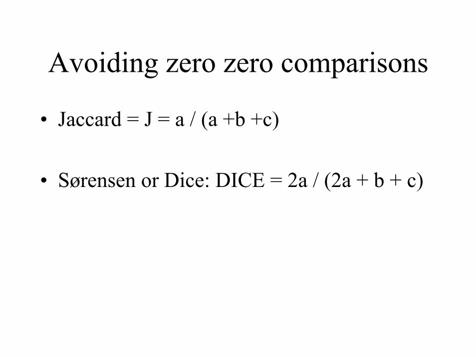
Avoiding zero zero comparisons

• Jaccard = J = a / (a +b +c)

• Sørensen or Dice: DICE = 2a / (2a + b + c)

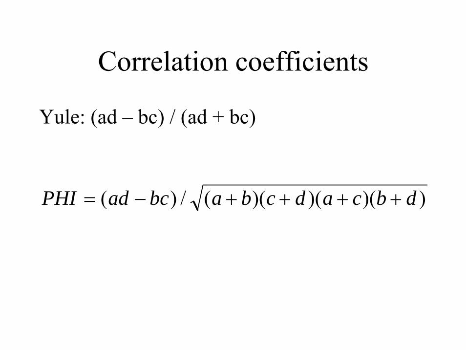
Correlation coefficients

Yule: (ad – bc) / (ad + bc)

))()()((/)( dbcadcbabcadPHI ++++−=

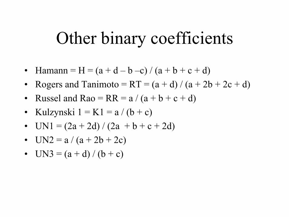
Other binary coefficients

• Hamann = H = (a + d – b –c) / (a + b + c + d)• Rogers and Tanimoto = RT = (a + d) / (a + 2b + 2c + d)• Russel and Rao = RR = a / (a + b + c + d) • Kulzynski 1 = K1 = a / (b + c)• UN1 = (2a + 2d) / (2a + b + c + 2d)• UN2 = a / (a + 2b + 2c)• UN3 = (a + d) / (b + c)

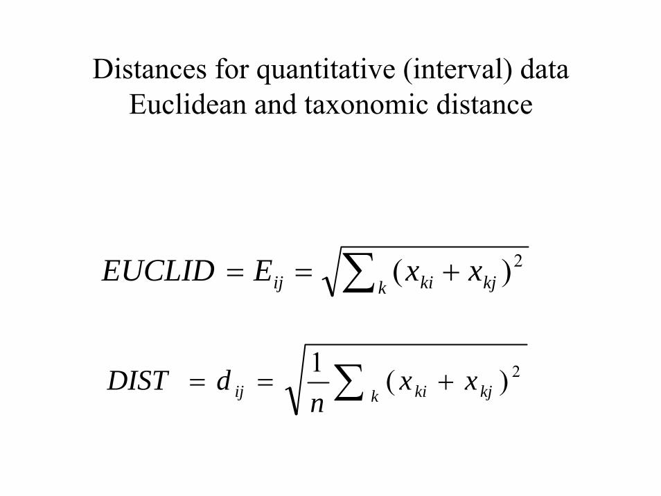
Distances for quantitative (interval) dataEuclidean and taxonomic distance

∑ +==k kjkiij xxEEUCLID 2)(

∑ +==k kjkiij xx

ndDIST 2)(1

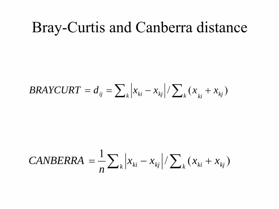
Bray-Curtis and Canberra distance

)(/ kjkikk kjkiij xxxxdBRAYCURT +−== ∑∑

)(/1 ∑∑ +−=k kjkik kjki xxxx

nCANBERRA

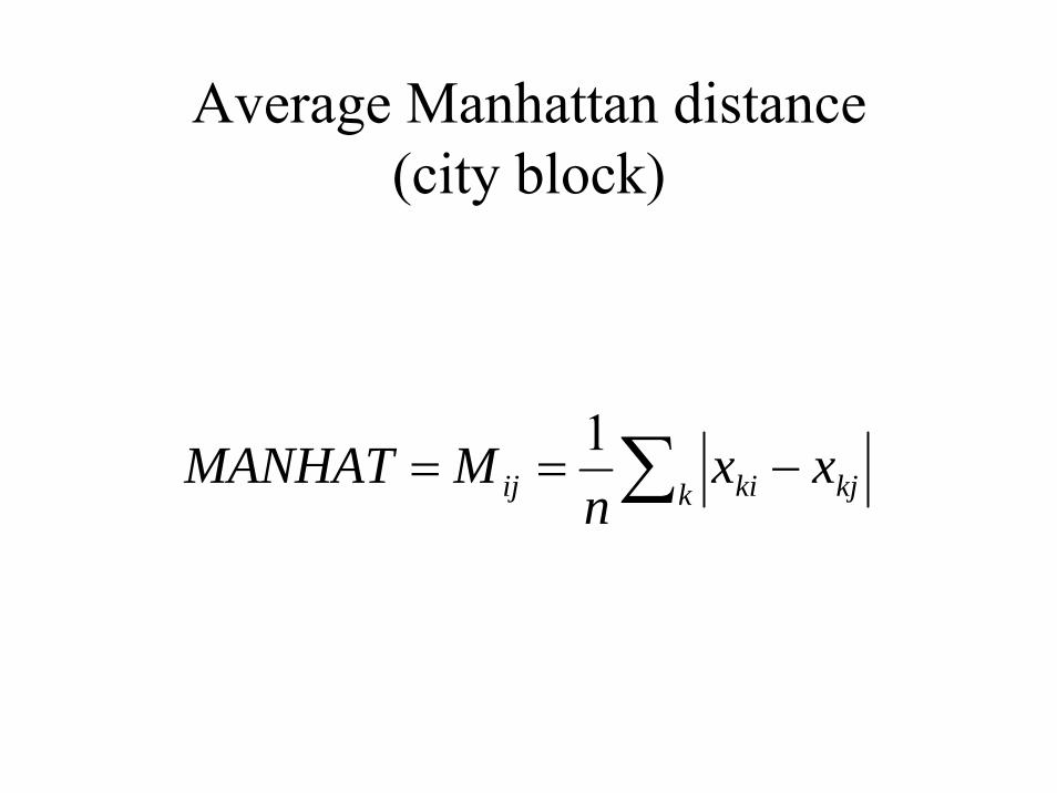
Average Manhattan distance(city block)

∑ −==k kjkiij xx

nMMANHAT 1

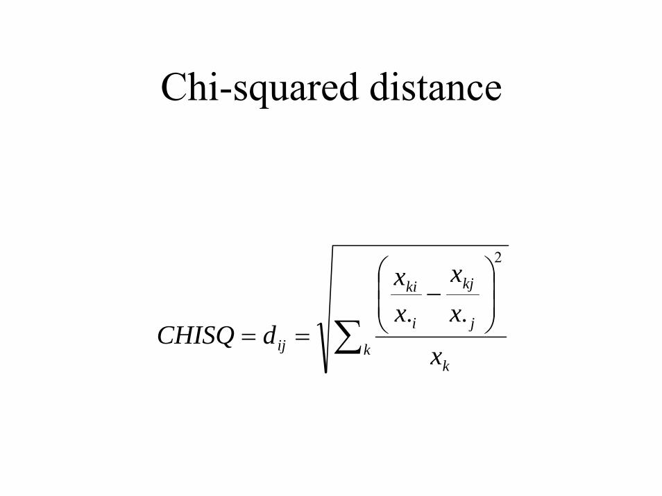
Chi-squared distance

∑⎟⎟⎠

⎞⎜⎜⎝

⎛−

==k

k

j

kj

i

ki

ij xxx

xx

dCHISQ

2

..

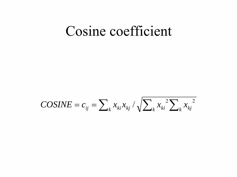
Cosine coefficient

∑ ∑∑==k k kjkikjk kiij xxxxcCOSINE 22/

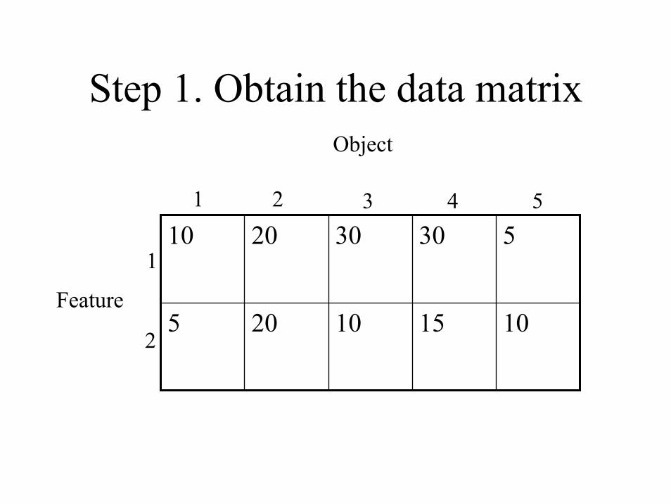
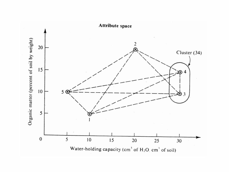
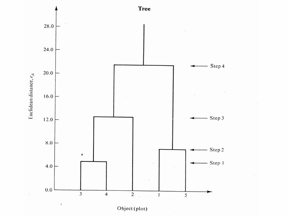
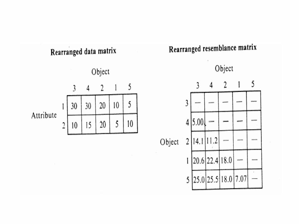
Step 1. Obtain the data matrix

10 20 30 30 5

5 20 10 15 10

Object

Feature

1

2

1 2 3 4 5

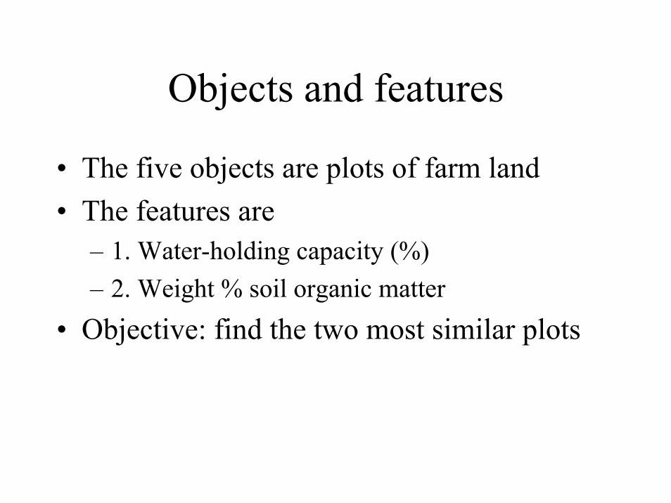
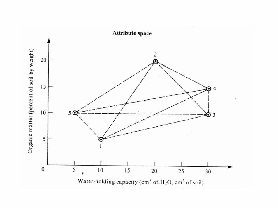
Objects and features

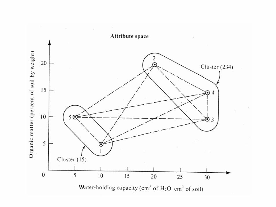
• The five objects are plots of farm land• The features are

– 1. Water-holding capacity (%)– 2. Weight % soil organic matter

• Objective: find the two most similar plots

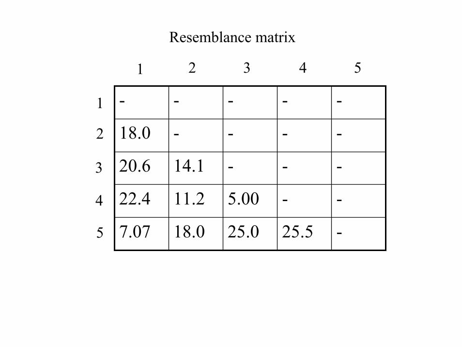
Resemblance matrix

- - - - -

18.0 - - - -

20.6 14.1 - - -

22.4 11.2 5.00 - -

7.07 18.0 25.0 25.5 -

1

2

3

4

5

1 2 3 4 5

- - - -

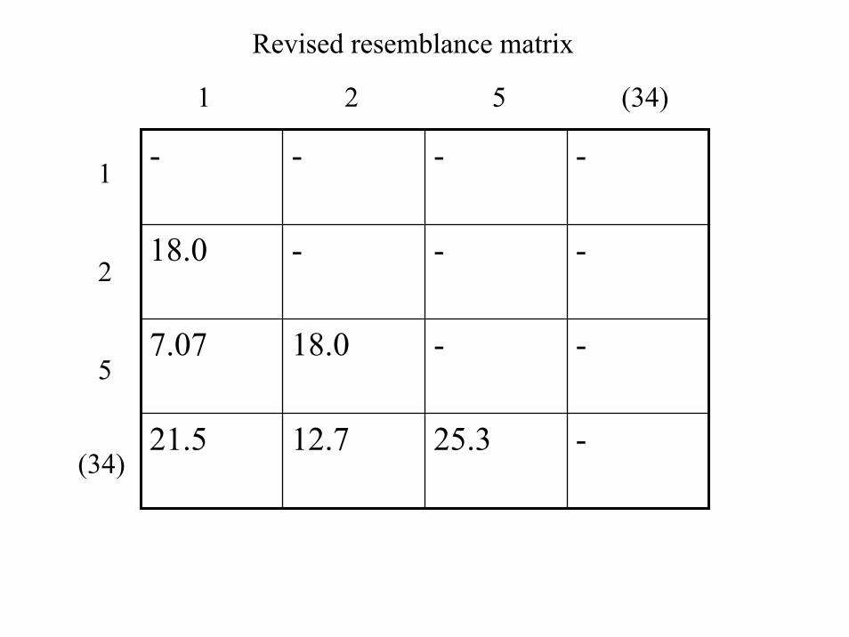
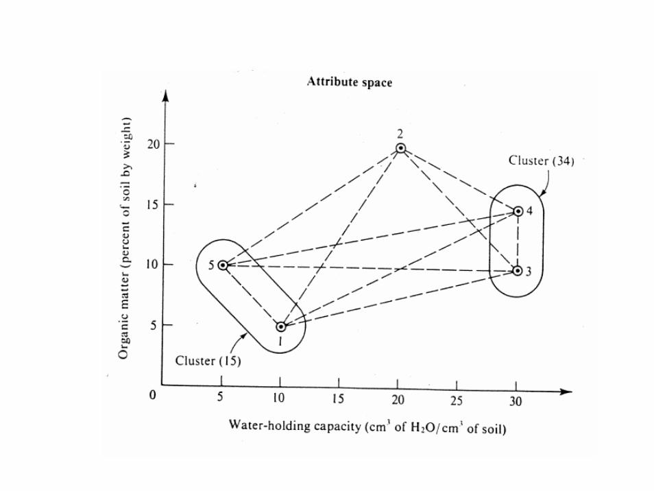
18.0 - - -

7.07 18.0 - -

21.5 12.7 25.3 -

1

2

5

(34)

1 2 5 (34)

Revised resemblance matrix

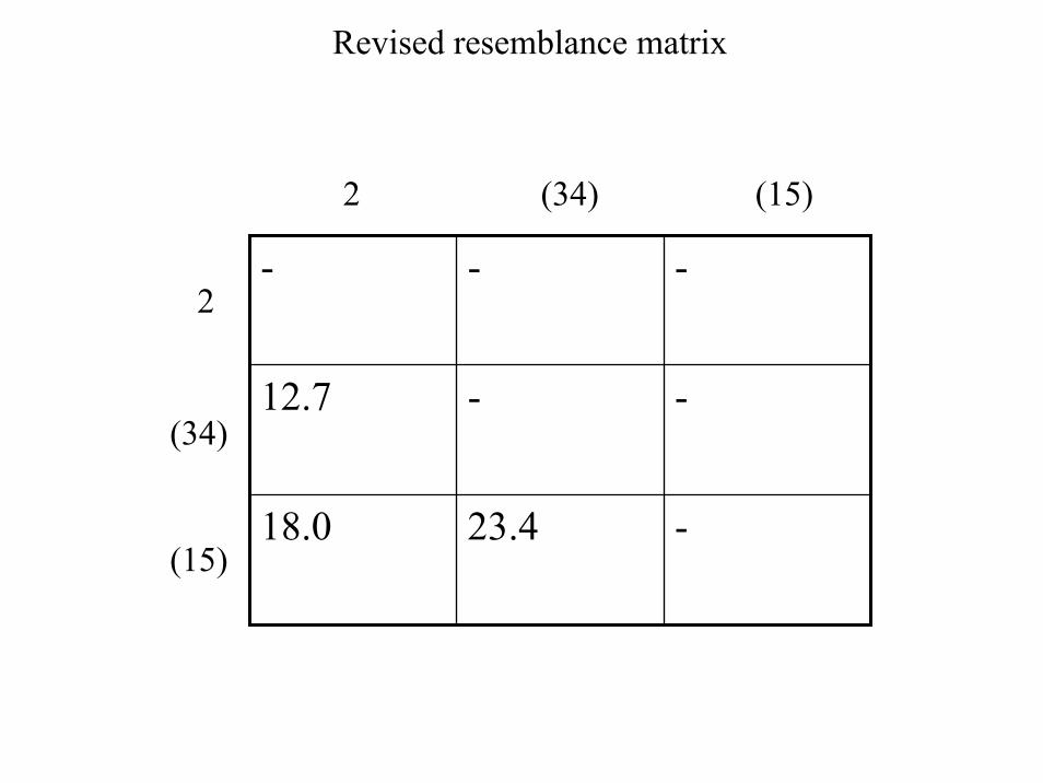
Revised resemblance matrix

- - -

12.7 - -

18.0 23.4 -

2

(34)

(15)

2 (34) (15)

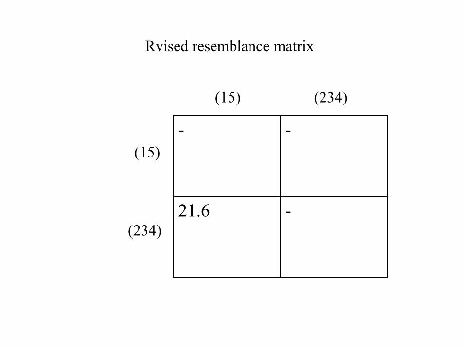
Rvised resemblance matrix

- -

21.6 -

(15)

(234)

(15) (234)

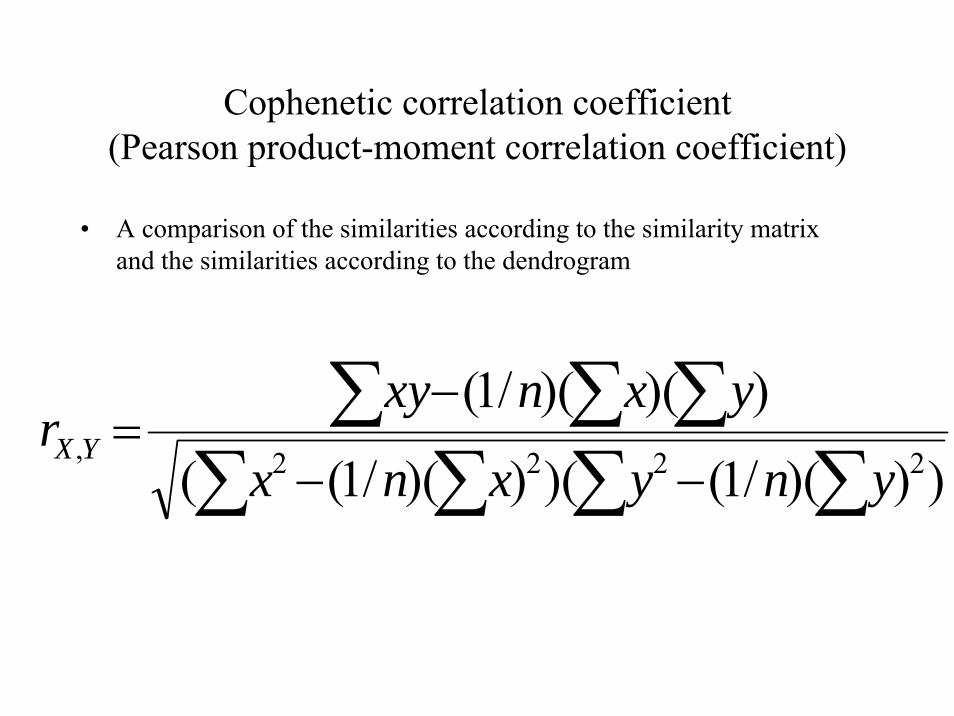
Cophenetic correlation coefficient(Pearson product-moment correlation coefficient)

• A comparison of the similarities according to the similarity matrix and the similarities according to the dendrogram

∑ ∑ ∑ ∑∑ ∑ ∑

−−

−=

)))(/1()())(/1((

))()(/1(2222,

ynyxnx

yxnxyr YX

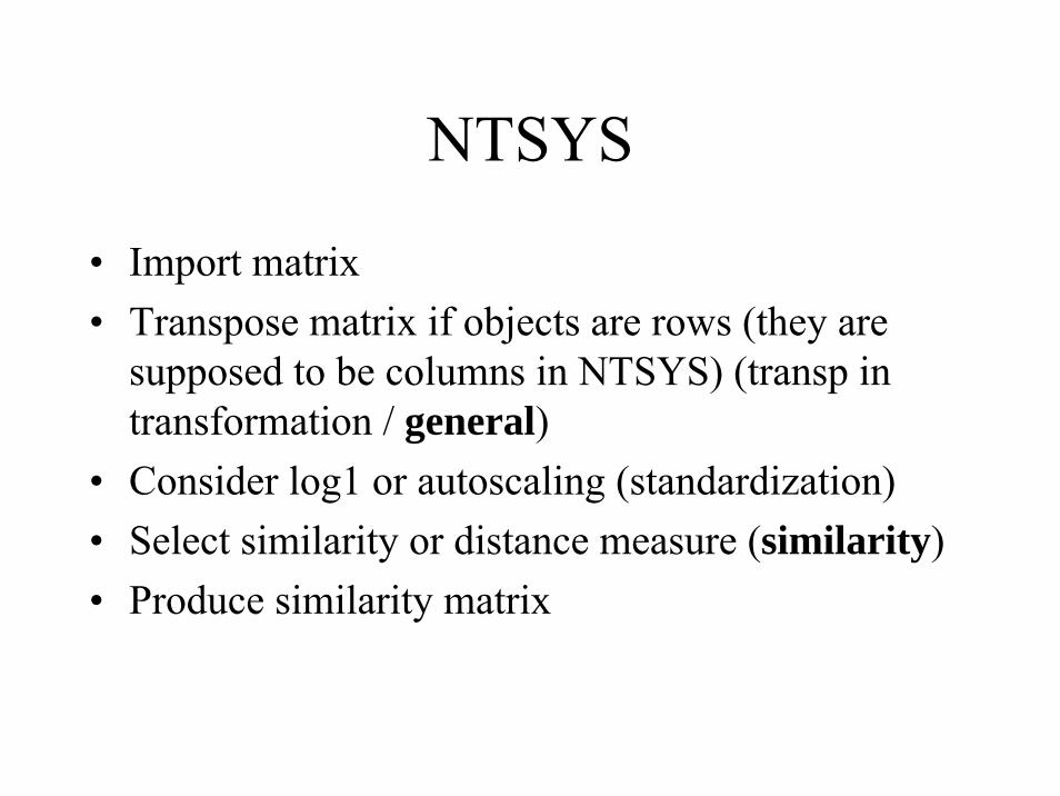
NTSYS

• Import matrix• Transpose matrix if objects are rows (they are

supposed to be columns in NTSYS) (transp in transformation / general)

• Consider log1 or autoscaling (standardization)• Select similarity or distance measure (similarity)• Produce similarity matrix

NTSYS (continued)

• Select clustering procedure (often UPGMA) (clustering)

• Calculate cophenetic matrix (clustering)• Compare similarity matrix with cophenetic

matix (made from the dendrogram) and write down the cophenetic correlation(graphics, matrix comparison)

• Write dendrogram (graphics, treeplot)