CLP-based protein fragment assembly

A. Dal Palu1, A. Dovier2, F. Fogolari3, and E. Pontelli4

1 Univ. Parma, Dip. di Matematica2 Univ. Udine, Dip. di Matematica e Informatica

3 Univ. Udine, Dip. di Scienze e Tecnologie Biomediche4 New Mexico State Univ., Dept. Maths and Computer Science

Abstract. The paper investigates a novel approach, based on Con-straint Logic Programming (CLP), to predict the 3D conformation ofa protein via fragments assembly. The fragments are extracted by apreprocessor—also developed for this work— from a database of knownprotein structures that clusters and classifies the fragments according tosimilarity and frequency. The problem of assembling fragments into acomplete conformation is mapped to a constraint solving problem andsolved using CLP. The constraint-based model uses a medium discretiza-tion degree Cα-side chain centroid protein model that offers efficiencyand a good approximation for space filling. The approach adapts ex-isting energy models to the protein representation used and applies alarge neighboring search strategy. The results show the feasibility andefficiency of the method. The declarative nature of the solution allowsto include future extensions, e.g. different size fragments for better ac-curacy.

1 Introduction

Proteins are central components in the way they control and execute the vitalfunctions in living organisms. The functions of a protein are directly related toits peculiar three-dimensional conformation. Knowledge of the three-dimensionalconformation of a protein (also known as the native conformation or tertiarystructure) is essential to biomedical investigation. The native conformation rep-resents the functional protein and determines how it can interact with otherproteins and affect the functions of the hosting organism. It is impossible toclearly understand the behavior and phenotype of an organism without knowl-edge of the native conformation of the proteins coded in its genome. As a resultof advancements in DNA sequencing techniques, there is a large and growingnumber of protein sequences—i.e., lists of amino acids, also known as primarystructures of proteins—available in public databases (e.g., the database Swiss-prot contains about 500, 000 protein sequences). On the other hand, knowledgeof structural information (e.g., information concerning the tertiary structures)is lagging behind, with a much smaller number of structures deposited in publicdatabases, notwithstanding structural genomics initiatives started worldwide.

For these reasons, one of the most traditional and central problems addressedby research in bioinformatics deals with the protein structure prediction problem,

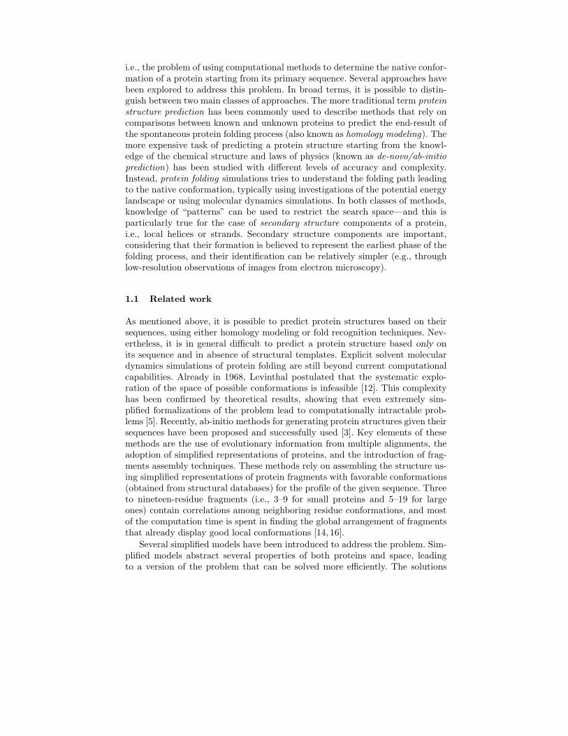
i.e., the problem of using computational methods to determine the native confor-mation of a protein starting from its primary sequence. Several approaches havebeen explored to address this problem. In broad terms, it is possible to distin-guish between two main classes of approaches. The more traditional term proteinstructure prediction has been commonly used to describe methods that rely oncomparisons between known and unknown proteins to predict the end-result ofthe spontaneous protein folding process (also known as homology modeling). Themore expensive task of predicting a protein structure starting from the knowl-edge of the chemical structure and laws of physics (known as de-novo/ab-initioprediction) has been studied with different levels of accuracy and complexity.Instead, protein folding simulations tries to understand the folding path leadingto the native conformation, typically using investigations of the potential energylandscape or using molecular dynamics simulations. In both classes of methods,knowledge of “patterns” can be used to restrict the search space—and this isparticularly true for the case of secondary structure components of a protein,i.e., local helices or strands. Secondary structure components are important,considering that their formation is believed to represent the earliest phase of thefolding process, and their identification can be relatively simpler (e.g., throughlow-resolution observations of images from electron microscopy).

1.1 Related work

As mentioned above, it is possible to predict protein structures based on theirsequences, using either homology modeling or fold recognition techniques. Nev-ertheless, it is in general difficult to predict a protein structure based only onits sequence and in absence of structural templates. Explicit solvent moleculardynamics simulations of protein folding are still beyond current computationalcapabilities. Already in 1968, Levinthal postulated that the systematic explo-ration of the space of possible conformations is infeasible [12]. This complexityhas been confirmed by theoretical results, showing that even extremely sim-plified formalizations of the problem lead to computationally intractable prob-lems [5]. Recently, ab-initio methods for generating protein structures given theirsequences have been proposed and successfully used [3]. Key elements of thesemethods are the use of evolutionary information from multiple alignments, theadoption of simplified representations of proteins, and the introduction of frag-ments assembly techniques. These methods rely on assembling the structure us-ing simplified representations of protein fragments with favorable conformations(obtained from structural databases) for the profile of the given sequence. Threeto nineteen-residue fragments (i.e., 3–9 for small proteins and 5–19 for largeones) contain correlations among neighboring residue conformations, and mostof the computation time is spent in finding the global arrangement of fragmentsthat already display good local conformations [14, 16].

Several simplified models have been introduced to address the problem. Sim-plified models abstract several properties of both proteins and space, leadingto a version of the problem that can be solved more efficiently. The solutions

of the simplified problem constitute candidate configurations that can be re-fined with more computationally intensive methods, e.g., molecular dynamicssimulations. Possible simplifications include the introduction of fixed sizes ofmonomers and bond lengths, the representation of monomers as simple points,and viewing the three-dimensional space as a discretized collection of points.In these simplified models, it is possible to view the protein folding problem asan optimization problem, aimed at determining conformations that minimize anenergy function. The energy function must be defined according to the simplifiedmodel adopted [4, 11]. Simplified energy models have been devised specifically tosolve large instances of the structure prediction problem using constraint solvingapproaches [1, 9].

In our own previous efforts, we have applied declarative programming ap-proaches, based on constraint solving, to address the problem. We built ourefforts on a discrete crystal lattice organization of the allowable points in thethree-dimensional space. This representation exploits the property that the dis-tance between the Cα atoms5 of two consecutive amino acids is relatively con-stant (3.8A). The problem is viewed as placing amino acids in the allowablepoints, in such a way that constraints encoding the mutual distances of aminoacids in the primary sequence are satisfied [6, 7]. The original framework has alsobeen expanded to support several types of global constraints, i.e., constraints de-scribing complex relationships among groups of amino acids. One of these con-straints is the rigid structure constraint—this constraint enables the represen-tation of known substructures (e.g., secondary structure components), reducingthe problem to the determination of an appropriate placement and rotation ofsuch substructures in the lattice space. The ability to use rigid structure con-straints has been shown to lead to dramatic reductions in the search space [8, 2].However, exploiting knowledge of real rigid substructures in a discrete lattice isinfeasible, due to the errors introduced by the approximations imposed by thediscretized representation of the search space. On the other hand, the use of aless constrained space model leads to search spaces that are intractable. Thesetwo considerations lead to the new approach presented in this work.

1.2 The contribution of this work

Some of the most successful approaches to protein folding build on the princi-ples of using substructures. The intuition is that, while the complete folding ofa protein may be unknown, it is likely that all possible substructures, if prop-erly chosen, can be found among proteins whose conformations are known. Thefolding can be constructed by exploiting relationships among substructures. Anotable example of this approach is represented by Rosetta [14]—an ab ini-tio protein structure prediction method that uses simulated annealing search tocompose a conformation, by assembling substructures extracted from a fragmentlibrary; the library is obtained from observed structures stored in the ProteinData Bank (PDB, www.pdb.org).

5 A carbon atom that is a convenient representative of the whole amino acid

In this work, we follow a similar idea, by developing a database of aminoacid chains of length 4; these are clustered according to similarity, and theirfrequencies are drawn from the investigation of a relevant section of the ProteinData Bank. The database contains the data needed to solve the protein foldingproblem via fragments assembly. Declarative programming techniques are usedto generate clean and compact code, and to enable rapid prototyping. Moreover,the problem of assembling substructures is efficiently tackled using the constraintsolving techniques provided by CLP (FD) systems.

This paper has the goal of showing that our approach is feasible. The mainadvantage, w.r.t. a highly engineered and imperative tool, is the modularity ofthe constraint system, which offers a convenient framework to test and integratestatistical data from various predictors and databases. Moreover, the constrainedsearch technique itself represents a novel method, compared to popular predic-tors, and we show its effectiveness in combination with the development of newenergy functions and heuristics. The proposed solution includes a general im-plementation of large neighboring search in CLP (FD), that turned out to behighly effective for the problem at hand. Another contribution is the develop-ment of a new energy function based on two components: a contact potentialfor backbone and side chain centroids interaction, and an energy component forbackbone conformational preferences. Backbone and side chain steric hindrancesare imposed as constraints.

2 Protein Abstraction

2.1 Preliminary notions

We focus on proteins described as sequences of amino acids selected from a setA of 20 elements (those coded by the human genome). In turn, each amino acidis composed of a set of atoms that constitute the amino acid’s backbone (seeFig. 1) and a set of atoms that differentiate pairs of amino acids, known as sidechain. One of the most important structural properties is that two consecutiveCα atoms have an average distance of 3.8A. Side chains may contain from 1 to18 atoms, depending on the amino acid. For computational purposes, insteadof considering all atoms composing the protein, we consider a simplified modelin which we are interested in the position of the Cα atoms (representing thebackbone of the protein) and of particular points, known as the centroids of theside chains (Fig. 3). A natural choice for the centroid is the center of mass ofthe side chain.

It is important to mention that, once the positions of all the Cα atoms andof all the centroids are known, the structure of the protein is already sufficientlydetermined, i.e., the position of the remaining atoms can be identified almostdeterministically with a reasonable accuracy.

Focusing on the backbone and on the Cα atoms, three consecutive aminoacids define one bend angle (see Fig. 2—left). Consider now four consecutiveamino acids a1, a2, a3, a4. The angle of the vector connecting a3 to a4 w.r.t. the

'

&

$

%

|sidechain

Cα

H

��NX

XXz

H

XX C′

O

��

��:

sidechain

'

&

$

%NXX

H

Cα|H

��C′

O

XXXz

ALA 7→ 0 LEU 7→ 1MET 7→ 1 ARG 7→ 2GLU 7→ 2 GLN 7→ 2LYS 7→ 2 ASN 7→ 3ASP 7→ 3 SER 7→ 3THR 7→ 4 PHE 7→ 4HIS 7→ 4 TYR 7→ 4ILE 7→ 5 VAL 7→ 5TRP 7→ 5 CYS 7→ 6GLY 7→ 7 PRO 7→ 8

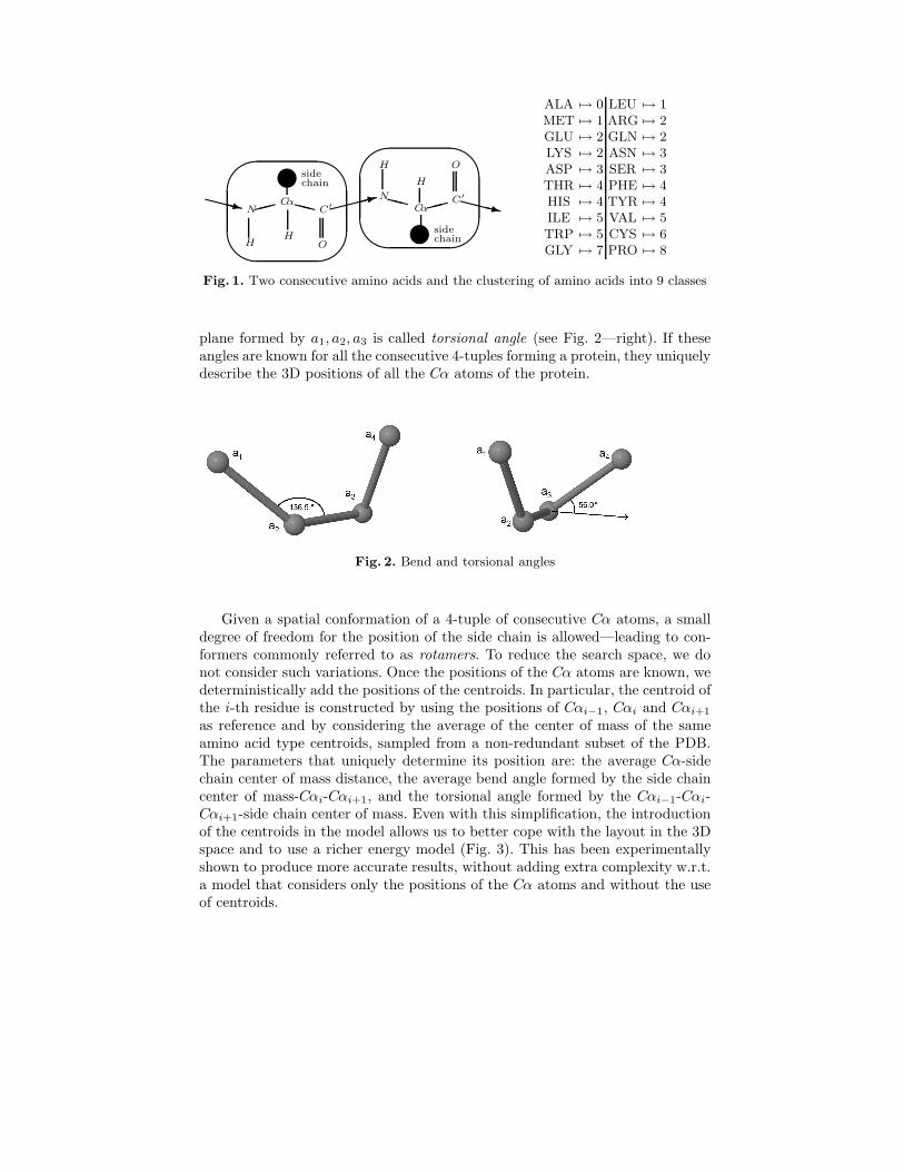
Fig. 1. Two consecutive amino acids and the clustering of amino acids into 9 classes

plane formed by a1, a2, a3 is called torsional angle (see Fig. 2—right). If theseangles are known for all the consecutive 4-tuples forming a protein, they uniquelydescribe the 3D positions of all the Cα atoms of the protein.

Fig. 2. Bend and torsional angles

Given a spatial conformation of a 4-tuple of consecutive Cα atoms, a smalldegree of freedom for the position of the side chain is allowed—leading to con-formers commonly referred to as rotamers. To reduce the search space, we donot consider such variations. Once the positions of the Cα atoms are known, wedeterministically add the positions of the centroids. In particular, the centroid ofthe i-th residue is constructed by using the positions of Cαi−1, Cαi and Cαi+1

as reference and by considering the average of the center of mass of the sameamino acid type centroids, sampled from a non-redundant subset of the PDB.The parameters that uniquely determine its position are: the average Cα-sidechain center of mass distance, the average bend angle formed by the side chaincenter of mass-Cαi-Cαi+1, and the torsional angle formed by the Cαi−1-Cαi-Cαi+1-side chain center of mass. Even with this simplification, the introductionof the centroids in the model allows us to better cope with the layout in the 3Dspace and to use a richer energy model (Fig. 3). This has been experimentallyshown to produce more accurate results, without adding extra complexity w.r.t.a model that considers only the positions of the Cα atoms and without the useof centroids.

Fig. 3. A fragment of 10 ALA amino acids in all-atom and Cα-centroid representation

2.2 Clustering

Although more than 60,000 protein structures are present in the PDB, the com-plete set of known proteins contains too much redundancy (i.e., very similarproteins deposited in several variants) to be useful for statistical purposes.

To reduce the impact of redundancy, in our approach, we focused on a subsetof the PDB with limited redundancies—in particular, we used the so-called top-

500 set [13].6 This set contains 500 proteins, with 107, 138 occurrences of aminoacids. The number of different 4-tuples occurring in the set is precisely 62, 831.Since the number of possible 4-tuples of amino acids is |A4| = 204 = 160, 000,this means that most 4-tuples do not appear in the selected set; even thosethat appear, occur too rarely to provide significant statistical information. Forthis reason, we decided to cluster amino acids into 9 classes, according to thesimilarity of the torsional angles of the pseudo bond between two consecutiveCα atoms [11]. Let γ : A −→ {0, . . . , 8} be the function assigning a class toeach amino acid, as defined in Fig. 1; for i ∈ {0, . . . , 8}, let us denote withγ−1(i) = {a ∈ A : γ(a) = i}. In this way, the majority of the 94 = 6, 5614-tuples have a representative in the set (precisely, there are templates for 5, 830of them).

A second level of approximation is introduced in deciding when two occur-rences of the same 4-tuple have the “same” form. The two tuples are placed inthe same class when their Root Mean Square Deviation (RMSD) is less than orequal to a given threshold (rmsd thr); this threshold is currently set to 1.0A.We developed a C program, called tuple generator, that creates a set of factsof the form:

tuple( [g1, g2, g3, g4],[Xα

1 , Y α1 , Zα

1 , Xα2 , Y α

2 , Zα2 , Xα

3 , Y α3 , Zα

3 , Xα4 , Y α

4 , Zα4 ],

g2-centroid-list, g3-centroid-list,

FREQ, ID, PID)

where [g1, g2, g3, g4] ∈ {0, . . . , 8}4 identifies the class of each amino acid, Xα1 , . . . , Zα

4

are the coordinates of the 4 Cα atoms of the 4-tuple,7 FREQ ∈ {0, . . . , 1000} is afrequency factor of the template w.r.t. all occurrences of the 4-tuple g1, . . . , g4 in

6 Note that our program tuple generator, developed to extract the desired informa-tion, can work on any given set of known proteins.

7 Without loss of generality, we set (Xα1 , Y

α1 , Z

α1 ) = (0, 0, 0).

the set top-500, ID is a unique identifier for this fact, and PID is the first proteinfound containing this template; this last piece of information will be printed inthe file we produce as output of the computation, in order to allow one to recoverthe source of a fragment used for the prediction.

As discussed in Sect. 2.1, we model the position of the centroid of the sidechain of every amino acid. gi ∈ {0, . . . , 8} is a representative of the class of aminoacids γ−1(gi) (e.g., γ−1(2) = {ARG, GLU, GLN, LYS}—see Fig. 1). For eachamino acid a ∈ γ−1(gi), we compute the position of the centroid corresponding tothe positions Xα

1 , . . . , Zα4 of the Cα atoms, and add it to the gi-centroid-list.

Let us observe that we do not add the position of the first and last centroid inthe 4-tuples. As a result, at the end of the computation, only the centroid of thefirst and the last amino acids of the entire protein will be not set; these can beassigned using a straightforward post-processing step.

It is unlikely that a 4-tuple a1, . . . , a4 that does not appear in the consideredtraining set will occur in a real protein. Nevertheless, in order to handle thesecases, if [γ(a1), . . . , γ(a4)] has no statistics associated to it, we map it to thespecial 4-tuple [−1,−1,−1,−1]. By default, we assign to this unknown tuple aset of templates (currently 6, but the number can be easily increased) chosenamong the most common ones in the set of all known templates. Other special 4-tuples are [−2,−2,−2,−2] and [−3,−3,−3,−3]; these are assigned to α-helicesand β-sheets every time a secondary structure constraint is enforced locally ona region of the conformation.

We also introduce an additional collection of facts, based on the predicatenext, which are used to relate pairs of tuple facts. The relation next(ID1, ID2, Mat)holds if the last three amino acids of the sequence in the tuple fact identifiedby ID1 are identical to the first three amino acids of the sequence in the tuple

fact ID2, and the corresponding Cα sequences are almost identical—in the sensethat the RMSD between them is at most rmsd thr. Mat is the rotation matrixto align the 1–3 Cα atoms of the 4-tuple of ID2 with the 2–4 Cα atoms of the4-tuple of ID1.

2.3 Statistical energy

The energy function used in this work builds on two components: (1) a contactpotential for side chain and backbone contacts and (2) an energy componentfor each backbone conformation based on backbone conformational preferencesobserved in the database. The first component uses the table of contact energiesdescribed in [4]. This set of energies has been shown to be accurate, and it isthe result of filtering the dataset to allow accurate statistical analysis, and aconsequent fine tuning of the contact definition. Since not all side chain atomsare represented, it is not possible to directly use the definition of [4]; therefore,we retain the table of contact energies of [4], but we adapt the contact definitionto the side chain centroid. In particular, we use the value 3.2A as the shortestdistance between two centroids, and we set the contact distance between twocentroids to be less than or equal to the sum of their radii. Larger distancesprovide a contribution that decays quadratically with the distance.

The radius of each centroid is computed as the centroid’s average distancefrom the Cα atom. No contact potential is assigned to the side chain’s Cα, asthe side chain definition already includes the Cα carbon. The energy assignedto the contact between backbone atoms represented by Cα (not included in theside chain definition) is the same energy assigned to ASN-ASN contacts, whichinvolve mainly similar chemical groups contacts. The torsional angle defined byfour consecutive Cα atoms is assigned an energy value defined by the potential ofthe mean force derived by the distribution of the corresponding torsional anglein the PDB. The procedure has been thoroughly described in [11].

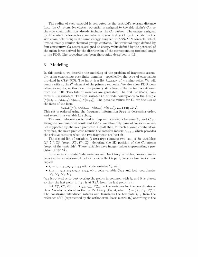
3 Modeling

In this section, we describe the modeling of the problem of fragments assem-bly using constraints over finite domains—specifically, the type of constraintsprovided in CLP (FD). The input is a list Primary of n amino acids. We willdenote with ai the ith element of the primary sequence. We also allow PDB iden-tifiers as inputs; in this case, the primary structure of the protein is retrievedfrom the PDB. Two lists of variables are generated. The first list (Code) con-tains n − 3 variables. The i-th variable Ci of Code corresponds to the 4-tuple(γ(ai), . . . , γ(ai+1), γ(ai+2), γ(ai+3)). The possible values for Ci are the IDs ofthe facts of the form

tuple([γ(ai), γ(ai+1), γ(ai+2), γ(ai+3)], , , Freq, ID, ).This set is ordered using the frequency information Freq in decreasing order,and stored in a variable ListDomi.

The next information is used to impose constraints between Ci and Ci+1.Using the combinatorial constraint table, we allow only pairs of consecutive val-ues supported by the next predicate. Recall that, for each allowed combinationof values, the next predicate returns the rotation matrix Mi,i+1, which providesthe relative rotation when the two fragments are best fit.

The second list of variables (Tertiary) contains two lists of 3n variables:Xα

i , Y αi , Zα

i (resp., XCi , Y C

i , ZCi ) denoting the 3D position of the Cα atoms

(resp., of the centroids). These variables have integer values (representing a pre-cision of 10−2A).

In order to correlate Code variables and Tertiary variables, consecutive 4-tuples must be constrained. Let us focus on the Cα part; consider two consecutivetuples:

• ti = ai, ai+1, ai+2, ai+3 with code variable Ci, and

• ti+1 = ai+1, ai+2, ai+3, ai+4, with code variable Ci+1 and local coordinatesV 1, V 2, V 3, V 4.

ti+1 is rotated as to best overlap the points in common with ti, and it is placedso that the last point in ti+1 is at 3.8A from the last point in ti.

Let Xαi , Y α

i , Zαi , . . . , Xα

i+4, Yαi+4, Z

αi+4 be the variables for the coordinates of

these Cα atoms, stored in the list Tertiary (Fig. 4, where Pi = (Xαi , Y α

i , Zαi )).

The constraint introduced rotates and translates the template ti+1 from thereference of Ci (represented by the orthonormal basis matrix Ri) according to the

rotation matrix Mi,i+1 to the new reference Ri+1 = Ri × Mi,i+1. Moreover, whenplacing the template ti+1, the constraint affects only the coordinates of ai+4,since the other variables are assigned by the application of the same constraintfor templates tj , j < i + 1. The constraint shifts the rotated version of ti+1

so that it overlaps the third point V 3 with (Xαi+3, Y

αi+3, Z

αi+3). Formally, let

Vrk = Ri+1 × V k, with k ∈ {1 . . . 4}, be the rotated 4-tuple corresponding to

Ci+1. The shift vector s = (Xαi+3, Y

αi+3, Z

αi+3) − V

r3 is used to constrain the

position of ai+4 as follows:(Xα

i+4, Yαi+4, Z

αi+4) = s + Ri+1 × V 4.

Note that the 3.8A distance between consecutive amino acids (i.e., ai+3 andai+4) is preserved, and this constraint allows us to place templates withoutrequiring an expensive RMSD fit among overlapping fragments during the search.Moreover, during a leftmost search, as soon as the variable Ci is assigned, alsothe coordinates (Xα

i+3, Yαi+3, Z

αi+3) are uniquely determined.

Matrix and vector products are handled by FD variables and constraints,using a factor of 1000 for storing and handling rotation matrices.

Fig. 4. Consecutive fragments combination

For the sake of simplicity, we omit the formal description of the constraintsassociated to the centroids. The centroids’ positions are determined similarly,e.g., as soon as the positions of the Cα atoms are determined, the centroidpositions are rotated and shifted accordingly.

The Xα1 , Y α

1 , Zα1 , . . . , Xα

n , Y αn , Zα

n part of the Tertiary list relative to theposition of the Cα atoms, is also required to satisfy a constraint which guaran-tees the all distant property [8]: the Cα atoms of each pair of non-consecutiveamino acids must be distant at least D = 3.2A. This is expressed by the con-straint:

(Xαi − Xα

j )2 + (Y αi − Y α

j )2 + (Zαi − Zα

j )2 ≥ D2

for all i ∈ {1, . . . , n− 2} and j ∈ {i + 2, . . . , n}. Similar constraints are imposedbetween pairs of Cα and centroids as well as pairs of centroids. In the latter case,in order to account for the differences in volume of each possible side chain, we

determine minimal distances that depend on the specific type of amino acidconsidered.

Other constraints are added to guide the search. We allow the user to seta diameter parameter that is used to bound the maximum distance betweendifferent Cα atoms (i.e., the diameter of the protein). As we argued in earlierwork [6], a good diameter value is 5.68 n0.38 A. We impose this constraint to alldifferent pairs of Cα atoms.

3.1 Secondary information

The native structure of a protein is largely composed of some recurrent localstructures. These structures, α-helices and β-sheets, can be predicted with goodaccuracy using efficient techniques, such as neural networks, or recognized usingother techniques (e.g., analysis of density maps from electron microscopy). Beingbased on frequency analysis, our tool is able to discover the majority of secondarystructures. On the other hand, a-priori knowledge of these structures allows usto remove several non-deterministic choices during computation. Therefore, weallow knowledge of secondary structures to be provided as part of the input—e.g.,information indicating that the amino acids i–j form an α-helix. In the processingstage, for k ∈ {i, . . . , j−3}, a particular tuple [−2,−2,−2,−2] is assigned insteadof the tuple [γ(ak), . . . , γ(ak+3)]. This tuple has a unique template which isassociated to an α-helix, built in a standard way using a bend angle of 93.8degrees and a torsional angle of 52.3 degrees. Moreover, a list of the possiblepositions for the centroids of the 20 amino acids is retrieved. Since the domainsfor these Ck’s are singletons, as soon as Ci is considered for value assignment,all the points of the helix are deterministically computed. The situation in thecase of β-strands is analogous.

A variation of this technique can be used if larger and more complex substruc-tures are known. Basically, even keeping just 4-tuples as internal data structures,we can easily deal with tuples of arbitrary lengths. Automated manipulation ofarbitrary complex structures is subject of future work.

4 Searching

The search is guided by the instantiation of the Ci variables. These variablesare instantiated in leftmost-first order; in turn, the values in their domains areattempted starting with the most probable value first. We observed that a first-fail strategy does not speed up the search, probably due to the weak propagationof the matrix product constraints. As described in Section 2.3, we associate anenergy to each computed structure. The energy value is an FD constraint thatlinks coordinates variables and amino acids. Given the model of the problem,this kind of constraint is not able to provide effective bounds for pruning thesearch space when searching for optimal solutions. As future work, we plan toinvestigate specific propagators, since the torsional energy contribution could beexploited for exact bounds estimations.

Each computed structure is saved in pdb format. This is a standard formatfor proteins (detailed in the PDB repository) that can be processed by mostprotein viewers (e.g., Rasmol, ViewerLite, JMol).

4.1 Large Neighboring Search

In order to further reduce the time to search for solutions, we have developeda logic programming implementation of Large Neighboring Search (LNS) [15].LNS is a form of local search, where the search for the successive solutions isperformed by exploring a “large” neighborhood. The traditional basic move usedin local search, where the values of a small number of variables are changed, isreplaced by a more general move, where a large number of variables is allowedto change, and these variables are subject to constraints. The basic LNS routineis the following:

1. Generate an initial solution (e.g., using the standard CLP labeling proce-dure).

2. Randomly select a subset of the variables of the problem that are admissiblefor changes, and assign the previous values to the other variables.

3. Using again standard labeling, look for an assignment of the selected vari-ables that improve the energy/cost function (or look for an assignment thatensures the best improvement possible of the energy/cost function). In anycase, go back to step 2.

A timeout mechanism is typically adopted to terminate the cycle between steps2 and 3. For example, the procedure is terminated if either a general time-outoccurs or k iterations are performed without any improvement in the quality ofthe solution. In these cases, the best solution found is returned.

This simple procedure can be improved by occasionally allowing a worseningmove—this is important to enable the procedure to abandon a local minimum.The process can be implemented by introducing a random variable; wheneversuch variable is assigned a certain value (with a low probability), then an alter-native move which worsens the quality of the solution is performed; otherwisewe continue using the scheme described earlier.

The scheme has been implemented in CLP (FD). Even though the imple-mentation has been developed to meet the needs of the protein folding problem,the scheme can be adapted with minimal changes to address the needs of otherconstraint optimization problems coded in CLP (FD). The logical variables ofCLP (FD), being single-assignment, are not suitable to the process of modifyinga solution as requested by LNS. Therefore, a specific combination of backtrack-ing, assertions and reassignment procedures are enforced, in order to reset onlythe assignments to the CSP (while the constraints are maintained) and to re-assign previous values to the variables that are not going to be changed. Theremaining variables can assume any assignment compatible with the constraints.

The implementation we developed avoids these repetitions, by using extra-logical features of Prolog to record intermediate solutions in the Prolog database(using the assert/retract predicates). The loss of declarativity is balanced byenhanced performance in the implementation of LNS.

Fig. 5 summarizes the CLP (FD) implementation of LNS. The predicate bestis used to memorize the best solution encountered, while the predicate last sol

represents the last solution found. The first clause of lns represents the core ofthe procedure—by setting up the constraints (constraint) and searching forsolutions (local); the fail at the end of the clause will cause backtracking intothe clauses of lns that determine the final result (lines 7-12). If at least onesolution has been found, then the final result is extracted from the fact of typebest in the database.

Starting from one solution (stored in the Prolog database in the fact last sol),the predicate another sol determines the next solution in the LNS process. If asolution has never been found, then a first solution is computed, by performinga labeling of the variables (lines 18-19). Otherwise, the values of some of thevariables are modified as dictated by LNS (line 24) and a new solution is com-puted. Note that an additional constraint on the resulting value of the objectivefunction (represented by the variable Energy) is added; with probability 1

10(as

determined by a random variable Type in line 21) a worsening of the energy isrequested (line 22), while in all other cases an improvement is requested (line23). If a new solution is found, this is recorded in the Prolog database (line 32);if this solution is better than any previous solution, then also the best fact isupdated (line 36). Observe that an internal time-out mechanism (set to 120s—line 25) is applied also on the search of a new solution. The “cut” in line 30 isintroduced to avoid the computation of another solution with the same randomchoices.

The iterations of another sol are performed by the predicate local (lines13-15). The negated call to another sol is necessary to enable removal of allvariable assignments (but saving constraints between variables) each time a newcycle is completed. The local procedure cycles indefinitely.

A final note on the procedure large move. We implemented two types ofLNS moves. The first (large pivot) makes a set of consecutive Code variablesunbound, allowing the procedure to change a (large) bend. The other Code vari-ables and the first segment of Tertiary variables remain assigned. The secondinstead leaves unbound two independent sets of consecutive variables, thus al-lowing a rotation of a central part of the protein (a sort of large crankshaft

move). We use both types of moves during the search (alternated using a randomselection process).

5 Experimental results

The prototype can search the first admissible solution (pf id(ID,Tertiary)),where ID is a protein name included in the database (prot list.pl); the Primarysequence is also admitted directly as input. It is possible to generate the first Nsolutions and output them as distinct models in a single pdb file, or to createdifferent files for all the solutions found within a Timeout. Finally, LNS can beactivated by pf id lns(ID,Timeout). A version of the current CLP (FD) im-

1: lns(ID, Time) :-

2: constraint(ID,Code,Energy,Primary,Tertiary),

3: retractall(best(_,_,_)), assert(best(0,Primary,_)),

4: retractall(last_sol(_,_,_)), assert(last_sol(0,null,_)),

5: time_out(local(Code,Energy,Primary,Tertiary), Time,_),

6: fail.

7: lns(_,_) :-

8: best(0,_,_,_),!,

9: write(’Insufficient time for the first solution’),nl.

10: lns(_,_) :-

11: best(Energy,Primary,Tertiary),

12: print_results(Primary,Tertiary,Energy).

13: local(Code,Energy, Primary,Tertiary):-

14: \+ another_sol(Code,Energy, Primary,Tertiary),

15: local(Code,Energy, Primary,Tertiary).

16: another_sol(Code, Energy, Primary, Tertiary) :-

17: last_sol(Lim, LastSol,LastTer),

18: ( LastSol = null ->

19: labeling(Code,Tertiary);

20: LastSol \= null ->

21: random(1,11,Type),

22: (Type =< 1 -> Lim1 is 5*Lim//6, Energy #> Lim1 ;

23: Type > 1 -> Energy #< Lim ),

24: large_move(Code,LastSol,Tertiary,LastTer),

25: time_out( labeling(Code,Tertiary), 120000, Flag)),

26: (Flag == success -> true ;

27: Flag == time_out ->

28: write(’Warning: Time out in the labeling stage’),nl,

29: fail)),

30: !,

31: retract(last_sol(_,_,_)),

32: assert(last_sol(Energy,Code,Tertiary)),

33: best(Val,_,_),

34: (Val > Energy ->

35: retract(best(_,_,_)),

36: assert(best(Energy,Primary,Tertiary));

37: true),

38: fail.

Fig. 5. An implementation of LNS in Prolog

plementation, along with a set of experimental tests, is available at www.dimi.

uniud.it/dovier/PF.

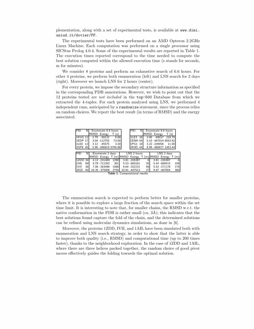
The experimental tests have been performed on an AMD Opteron 2.2GHzLinux Machine. Each computation was performed on a single processor usingSICStus Prolog 4.0.4. Some of the experimental results are reported in Table 1.The execution times reported correspond to the time needed to compute thebest solution computed within the allowed execution time (s stands for seconds,m for minutes).

We consider 8 proteins and perform an exhaustive search of 6.6 hours. Forother 4 proteins, we perform both enumeration (left) and LNS search for 2 days(right). Moreover we launch LNS for 2 hours (center).

For every protein, we impose the secondary structure information as specifiedin the corresponding PDB annotations. However, we wish to point out that the12 proteins tested are not included in the top-500 Database from which weextracted the 4-tuples. For each protein analyzed using LNS, we performed 4independent runs, anticipated by a randomize statement, since the process relieson random choices. We report the best result (in terms of RMSD) and the energyassociated.

PID N Enumerate 6.6 hoursRMSD Energy T (s)

1KVG 12 2.79 -59122 9.881EDP 17 3.04 -112755 73.001LE0 12 3.12 -45575 3.202GP8 40 5.96 -266819 5794.88

PID N Enumerate 6.6 hoursRMSD Energy T (s)

1LE3 16 3.90 -69017 218.791ENH 54 5.10 -467014 8553.921PG1 18 3.22 -109456 11.002K9D 44 6.99 -460877 1453.44

PID N Enumerate 2 days LNS 2 hours LNS 2 daysRMSD Energy T (m) RMSD Energy T (m) RMSD Energy T (m)

1ZDD 34 4.12 -231469 1290 3.81 -226387 6 3.81 -226387 61AIL 69 9.78 -711302 301 5.53 -665161 20 5.44 -668415 1091VII 36 7.06 -263496 1086 6.64 -252231 48 5.52 -271178 1702IGD 60 16.35 -375906 2750 10.91 -447513 27 8.67 -467004 380

Table 1. Computational results

The enumeration search is expected to perform better for smaller proteins,where it is possible to explore a large fraction of the search space within the settime limit. It is interesting to note that, for smaller chains, the RMSD w.r.t. thenative conformation in the PDB is rather small (ca. 3A); this indicates that thebest solutions found capture the fold of the chain, and the determined solutionscan be refined using molecular dynamics simulations, as done in [6].

Moreover, the proteins 1ZDD, IVII, and 1AIL have been simulated both withenumeration and LNS search strategy, in order to show that the latter is ableto improve both quality (i.e., RMSD) and computational time (up to 200 timesfaster), thanks to the neighborhood exploration. In the case of 1ZDD and 1AIL,where there are three helices packed together, the random choice of good pivotmoves effectively guides the folding towards the optimal solution.

Finally, the protein 2IGD shows that the allowed time was not sufficient todetermine a sensible prediction, even though the LNS shows enhancements inquality of the prediction, given the same amount of time. In this case, additionalwork is needed to improve the choice of moves performed by LNS, in order toexplore the neighborhood in a more effective way. For example, moves that shiftand translate some rigid parts of the protein may improve the performance andquality.

We also note that the size of the set of fragments in use is sufficient to allowreasonable solutions, while allowing tractable search spaces. Clearly, the use ofa more refined partitioning of the fragments (by reducing the rmsd thr) wouldproduce conformations that are structurally closer to the native state, at theprice of an increase in the size of the search space.

Fig. 6. Protein 1ENH: native state (left), prediction—green/light gray — compared tooriginal — red/dark grey— (center), prediction (right)

In Figure 6, we depict the native state (on the left) and our best prediction(on the right) for the protein 1ENH with the backbone and centroids. In themiddle, we show the RMSD overlap of the Cα atoms between the native confor-mation (red/dark gray) and the prediction (green/light gray). The main featuresare preserved and only the right loop that connects the two helices appears tohave moved significantly. This could be avoided by introducing a richer set ofalternative fragments in that area and thus allow a more relaxed placement ofthe fragments.

An important issue is that it is not obvious that the reduced representationand the energy function used here are able to distinguish the native structurefrom decoys constructed to minimize that energy function. The straightforwardcomparison between RMSD and energy is not completely meaningful because thenative structure should be energy-minimized before energy comparison. This canbe noted by comparing the conformations obtained by enumeration and LNS.The model in use improves w.r.t. the Cα model as presented in [6]. However,some fine tuning of the energy coefficients is still necessary in order to improvethe correlation, while preserving the overall constraint model. This will be afurther area of investigation. Our results show that the method can scale welland that further speed-up may be obtained by considering larger fragments asdone by tools like Rosetta. Rosetta is in fact the state-of-the-art predictor tool

(e.g., the small protein 1ENH is predicted by Rosetta in less than one minutewith a RMSD of 4.2 A).

6 Conclusions and future work

In this paper we presented the design and implementation of a constraint logicprogramming tool to predict the native conformation of a protein, given its pri-mary structure. The methodology is based on a process of fragments assembly,using templates retrieved from a protein database, that is clustered accordingto shape similarity. We used templates based on sequences of 4 amino acids,but longer sequences could be easily incorporated—and these could bring statis-tically significant constraints describing conserved shapes. The constraint solv-ing process takes advantage of a large neighboring search strategy, which hasbeen shown to be particularly effective when dealing with longer proteins. Thepreliminary experimental results confirm the strong potential for this fragmentassembly scheme.

The proposed method has a significant advantage over schemes like Rosetta—the use of CLP (FD) enables the simple addition of ad-hoc constraints and ex-perimentation with different local search moves and energy functions. As futurework, we plan to investigate, in particular, energy functions that better correlatewith RMSD w.r.t. the (known) native structures and the computed structures.Other (possibly redundant) constraints and constraint propagation techniquesshould be analyzed, possibly moving to the C++ solver Gecode.

Acknowledgments. The work is supported by GNCS-INdAM grant “Tecnicheinnovative per la programmazione con vincoli in applicazioni strategiche”, PRIN2007 “Computer simulations of Glutathione Peroxidases: insights into the cat-alytic mechanism” and PRIN 2008 “Innovative multi-disciplinary approaches forconstraint and preference reasoning” grants.

References

1. R. Backofen and S. Will. A Constraint-Based Approach to Fast and Exact Struc-ture Prediction in 3-Dimensional Protein Models. Constraints 11(1):5–30, 2006.

2. P. Barahona and L. Krippahl. Constraint Programming in Structural Bioinformat-ics. Constraints 13(1–2):3–20, 2008.

3. M. Ben-David, et al. Assessment of CASP8 structure predictions for template freetargets. Proteins 77(S9):50–65, 2009.

4. M. Berrera et al. Amino acid empirical contact energy definitions for fold recogni-tion in the space of contact maps. BMC Bioinformatics, 4(8), 2003.

5. P. Crescenzi et al. On the complexity of protein folding. STOC :61–62, 1998.6. A. Dal Palu, A. Dovier, and F. Fogolari. Constraint logic programming approach

to protein structure prediction. BMC Bioinformatics, 5(186), 2004.7. A. Dal Palu, A.Dovier, and E. Pontelli. A constraint solver for discrete lattices, its

parallelization, and application to protein structure prediction. Software: Practice

and Experience 37(13):1405–1449, 2007.

8. A. Dal Palu, A. Dovier, E. Pontelli. Computing Approximate Solutions of theProtein Structure Determination Problem using Global Constraints on DiscreteCrystal Lattices. International Journal of Data Mining and Bioinformatics 4(1):1–20, January 2010.

9. I. Dotu et al. Protein Structure Prediction with Large Neighborhood ConstraintProgramming Search. CP, LNCS 5202, pp. 82–96, 2008.

10. F. Fogolari et al. Modeling of polypeptide chains as C-α chains, C-α chains withC-β, and C-α chains with ellipsoidal lateral chains. Biophysical Journal, 70:1183–1197, 1996.

11. F. Fogolari et al. Scoring predictive models using a reduced representation ofproteins: model and energy definition. BMC Structural Biology, 7(15), 2007.

12. C. Levinthal. Are there pathways in protein folding? J. Chim. Phys. 65:44–45,1968.

13. S. Lovell, et al. Structure validation by Cα geometry: φ, ψ and Cβ deviation.Proteins 50:437–450, 2003.

14. S. Raman, et al. Structure prediction for CASP8 with all-atom refinement usingRosetta. Proteins 77(S9):89–99, 2009.

15. P. Shaw. Using Constraint Programming and Local Search Methods to SolveVehicle Routing Problems. Proc. of CP’98, LNCS 1520, pp. 417–431, 1998.

16. S. Wu, J. Skolnick, and Y. Zhang Ab initio modeling of small proteins by iterativeTASSER simulations. BMC Biology, 5(17), 2007.