CloudSat’s Cloud Profiling Radar (CPR): status, performance and new products

S. Tanelli, S.L. Durden and G. Dobrowalski Jet Propulsion Laboratory

CloudSat/CALIPSO STM, Madison, WI, July 28 2009

2

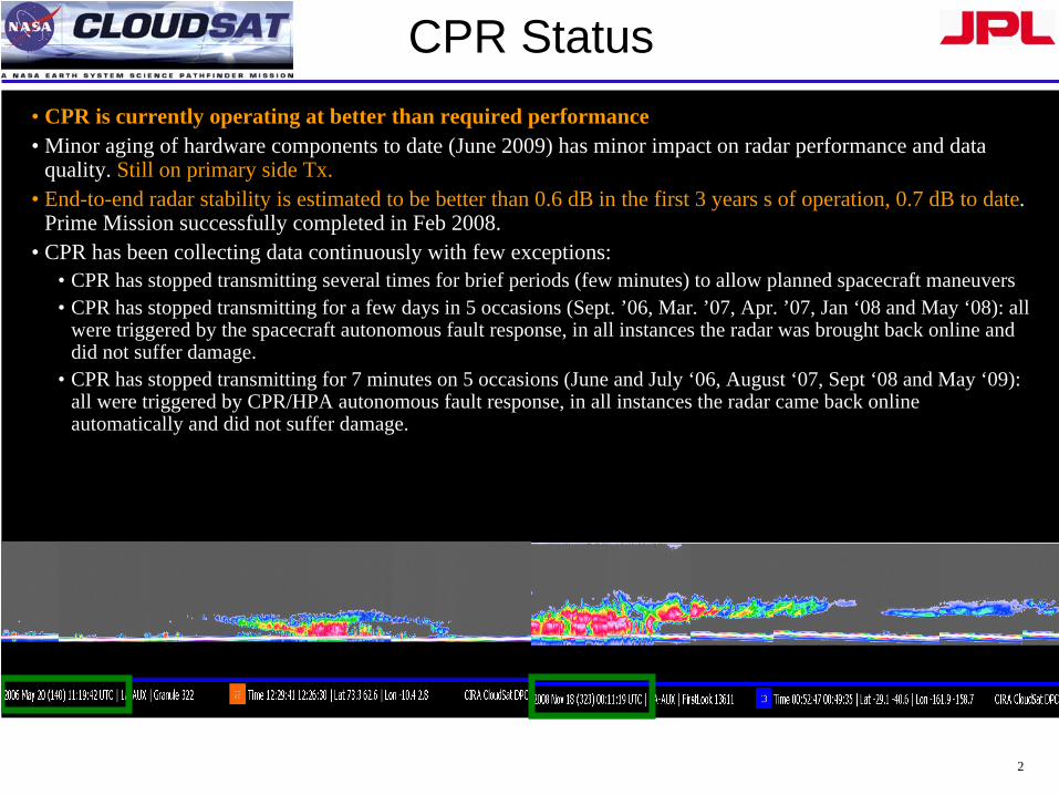
• CPR is currently operating at better than required performance• Minor aging of hardware components to date (June 2009) has minor impact on radar performance and data

quality. Still on primary side Tx.• End-to-end radar stability is estimated to be better than 0.6 dB in the first 3 years s of operation, 0.7 dB to date.

Prime Mission successfully completed in Feb 2008.• CPR has been collecting data continuously with few exceptions:

• CPR has stopped transmitting several times for brief periods (few minutes) to allow planned spacecraft maneuvers • CPR has stopped transmitting for a few days in 5 occasions (Sept. ’06, Mar. ’07, Apr. ’07, Jan ‘08 and May ‘08): all

were triggered by the spacecraft autonomous fault response, in all instances the radar was brought back online and did not suffer damage.

• CPR has stopped transmitting for 7 minutes on 5 occasions (June and July ‘06, August ‘07, Sept ‘08 and May ‘09): all were triggered by CPR/HPA autonomous fault response, in all instances the radar came back online automatically and did not suffer damage.

CPR Status

3

• Avg Orbital Transmit power as measured by calibrator has fluctuated ~ 0.7 dB (as of May 2009)

• During the first two years, apparent drop in Pt corresponds to an apparent increase in surface back scatter ( >0.95 correlation) - Best estimate is that actual transmit power, and receiver gain have been stable to better than 0.4 dB during Prime Mission. See IEEE TGRS Tanelli et al. 2008.

σ 0 =Pr

Pt

Cr2Δ

=σ ref0 /σ 0 = Pt /Pt,ref

Wind Speed (AMSR-E est) [m/s]

Wind Speed (AMSR-E est) [m/s]

<σ0 / σ0

,ref>

Std(σ0

)

CPR End-to-End Stability

Prime Mission

CPR Calibration/Validation

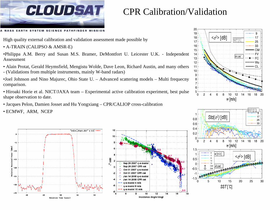
High quality external calibration and validation assessment made possible by• A-TRAIN (CALIPSO & AMSR-E)•Philippa A.M. Berry and Susan M.S. Bramer, DeMontfort U. Leicester U.K. - Independent Assessment• Alain Protat, Gerald Heymsfield, Mengistu Wolde, Dave Leon, Richard Austin, and many others - (Validations from multiple instruments, mainly W-band radars)•Joel Johnson and Nino Majurec, Ohio State U. – Advanced scattering models – Multi frequecny comparison.• Hiroaki Horie et al. NICT/JAXA team – Experimental active calibration experiment, best pulse shape observation to date.• Jacques Pelon, Damien Josset and Hu Yongxiang – CPR/CALIOP cross-calibration • ECMWF, ARM, NCEP

5

Surface Backscattering modeling advancement

• Cloud Sat data are being used to analyze and improve modeling of surface backscatter. Should coordinate with CALIPSO team. Two posters in this worshop:• Durden et al.• Majurec et al.

6

Transmitter Switchover Plan

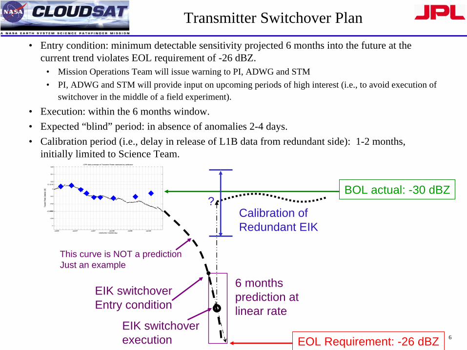
• Entry condition: minimum detectable sensitivity projected 6 months into the future at the current trend violates EOL requirement of -26 dBZ.

• Mission Operations Team will issue warning to PI, ADWG and STM• PI, ADWG and STM will provide input on upcoming periods of high interest (i.e., to avoid execution of

switchover in the middle of a field experiment).

• Execution: within the 6 months window.• Expected “blind” period: in absence of anomalies 2-4 days.• Calibration period (i.e., delay in release of L1B data from redundant side): 1-2 months,

initially limited to Science Team.

BOL actual: -30 dBZ

EOL Requirement: -26 dBZ

6 months prediction at linear rate

EIK switchoverEntry condition

This curve is NOT a predictionJust an example

EIK switchoverexecution

?Calibration ofRedundant EIK

7

CPR as Radiometer

• CPR noise power converted into brightness temperature using relationship obtained by comparing with AMSR-E 89-GHz TB

• Preliminary estimation of NEΔT ≅

5K

• Cold background (ocean) appears warmer in the presence of water cloud

Ocean, clear sky (Jan 1-17, 2007)

Ocean, cloudy sky (Jan 1-17, 2007) Land, cloudy sky (Jan 1-17, 2007)

Land, clear sky (Jan 1-17, 2007)

8

CPR as Radiometer

9

Tb product: step 1• Calculate CPR noise from L1B-CPR ReceivedEchoPowers

• Use L2B Cloud Mask and sem_noise_floor to flag ‘cloudy bins’ in the ‘noise region’.

• Iter #1: 4-sigma above mean• Iter #2: 3-sigma away from mean

• Option (Flag all bins beyond #85 in GEOPROF (i.e., lowest 5 km))

• Option (Flag all bins with Lidar echo)• Use all unflagged bins to calculate mean noise of each

ray• Filter CPR 1-ray noise along track

• Apply moving average filter with 6 window sizes, (1, 5, 11, 31, 61, 101)

• Adopt largest window in which noise population is distributed according to expectation.

• Convert noise to Brightness Temperature:• TB94 = filtered_noise * C1 + C2• C1 = 189 1015

• C2 = -670• Coefficients calculated from AMSR-E 89H Tb, Ws,

SST, and WVmm using lookup table• Tb 89H 55˚

--> Tb 94 0.16˚

with 1-D Radiative Transfer over ocean and clear air (Eddington Approximation)

10

Step 1: zoom in

11

Tb product: step 2• Calculate CPR noise from L1B-CPR ReceivedEchoPowers

• Use L2B Cloud Mask and sem_noise_floor to flag ‘cloudy bins’ in the ‘noise region’.

• Iter #1: 4-sigma above mean• Iter #2: 3-sigma away from mean

• Option (Flag all bins beyond #85 in GEOPROF (i.e., lowest 5 km))

• Option (Flag all bins with Lidar echo)• Use all unflagged bins to calculate mean noise of each

ray• Filter CPR 1-ray noise along track

• Apply moving average filter with 6 window sizes, (1, 5, 11, 31, 61, 101)

• Adopt largest window in which noise population is distributed according to expectation.

• Convert noise to Brightness Temperature:• TB94 = filtered_noise * C1 + C2• C1 = 189 1015

• C2 = -670• Coefficients calculated from AMSR-E 89H Tb, Ws,

SST, and WVmm using lookup table• Tb 89H 55˚

--> Tb 94 0.16˚

with 1-D Radiative Transfer over ocean and clear air (Eddington Approximation)

12

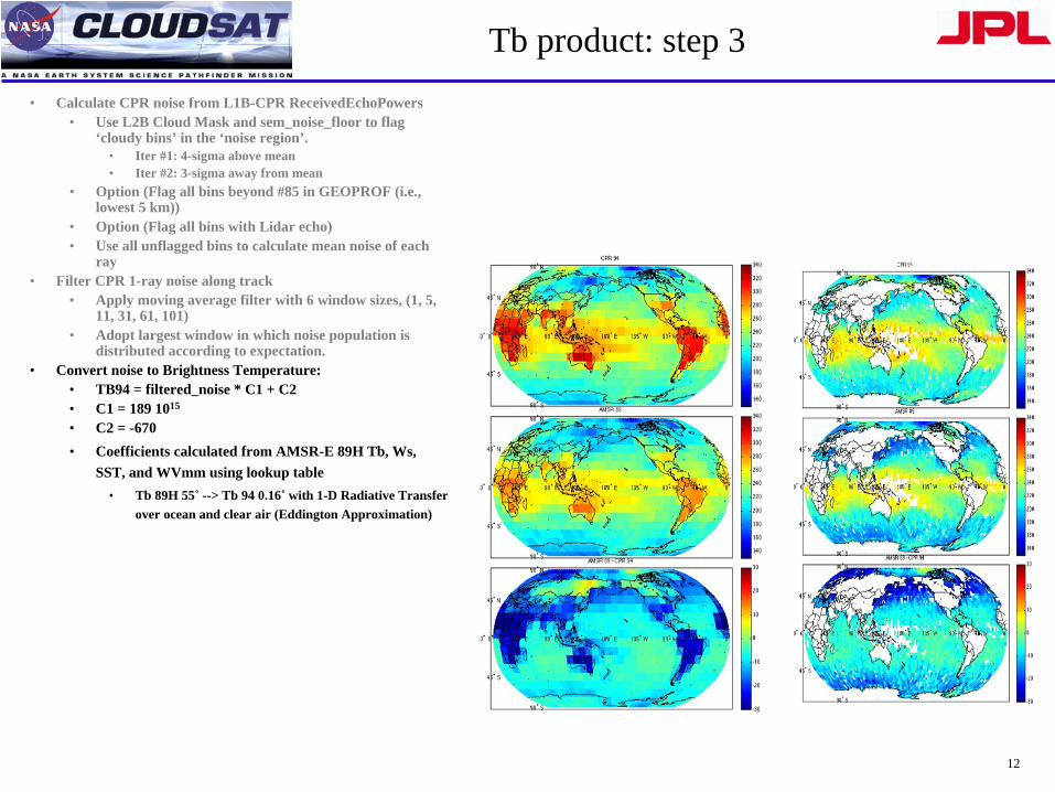
Tb product: step 3• Calculate CPR noise from L1B-CPR ReceivedEchoPowers

• Use L2B Cloud Mask and sem_noise_floor to flag ‘cloudy bins’ in the ‘noise region’.

• Iter #1: 4-sigma above mean• Iter #2: 3-sigma away from mean

• Option (Flag all bins beyond #85 in GEOPROF (i.e., lowest 5 km))

• Option (Flag all bins with Lidar echo)• Use all unflagged bins to calculate mean noise of each

ray• Filter CPR 1-ray noise along track

• Apply moving average filter with 6 window sizes, (1, 5, 11, 31, 61, 101)

• Adopt largest window in which noise population is distributed according to expectation.

• Convert noise to Brightness Temperature:• TB94 = filtered_noise * C1 + C2• C1 = 189 1015

• C2 = -670• Coefficients calculated from AMSR-E 89H Tb, Ws,

SST, and WVmm using lookup table• Tb 89H 55˚

--> Tb 94 0.16˚

with 1-D Radiative Transfer over ocean and clear air (Eddington Approximation)

13

Parameters used to find constants via lookup table

From AMSR-E• TB89H• Water vapor• Wind Speed• Sea Surface Temperature

14

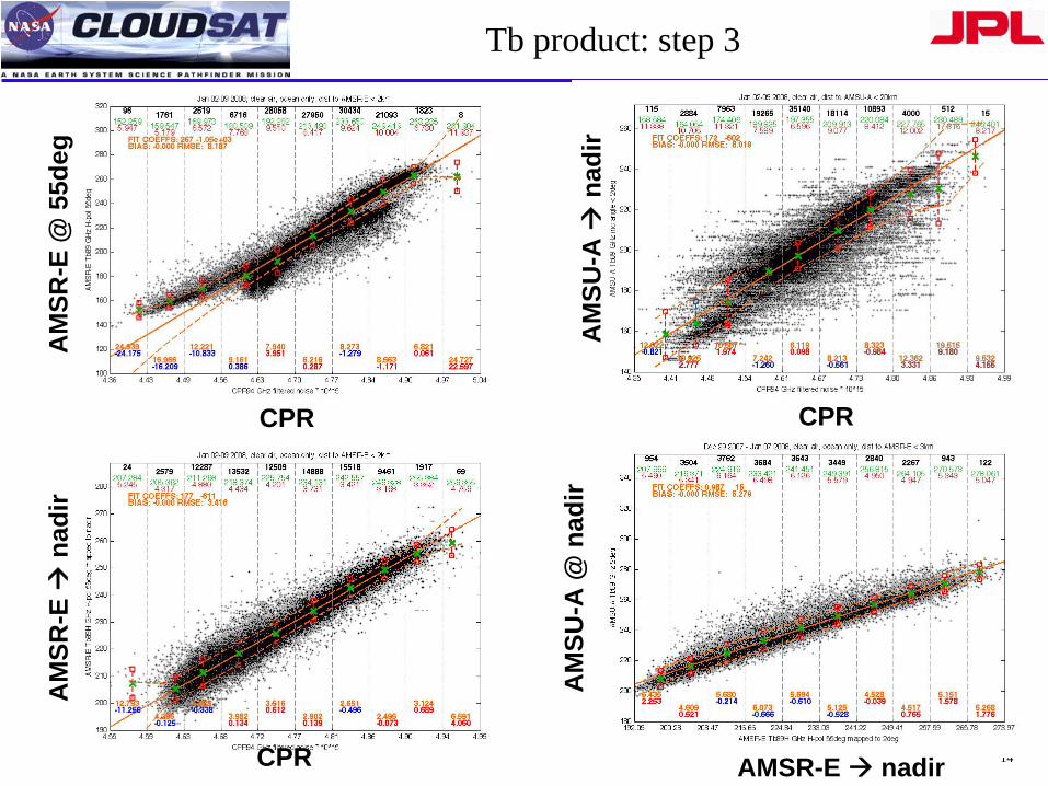
Tb product: step 3

CPR CPR

CPR AMSR-E nadir

AM

SU-A

@ n

adir

AM

SU-A

na

dir

AM

SR-E

@ 5

5deg

AM

SR-E

na

dir

15

Tb Product Status

• Code has been test run over several periods by the DPC• Will be distributed for more testing• Data will be added to 2B-GEOPROF output and stored in separate product

file (name TBD) with R05• Single ray noise avg• Single ray number of noise bins• Single ray noise std dev• Filter window size

16

Jan 2008 <Tb> = 242.741

Jan 2009 <Tb> = 239.401

Temporal drift due to Receiver Gain drift

17

Jan & Jul TKW -CLR ocean avg =5.6477

18

Jan & Jul TNW -CLR

19

20

21

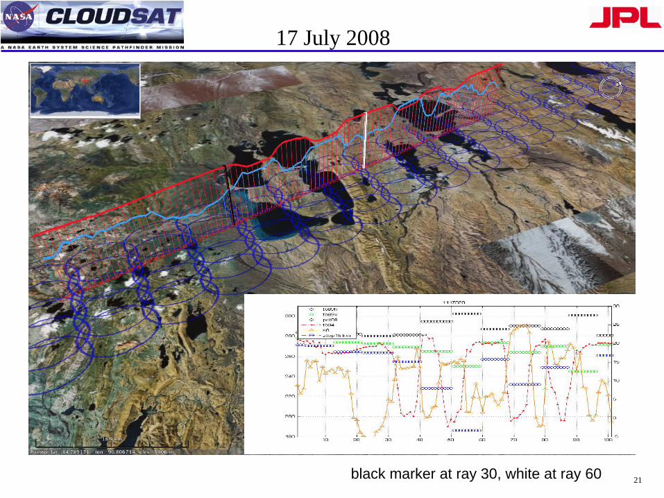
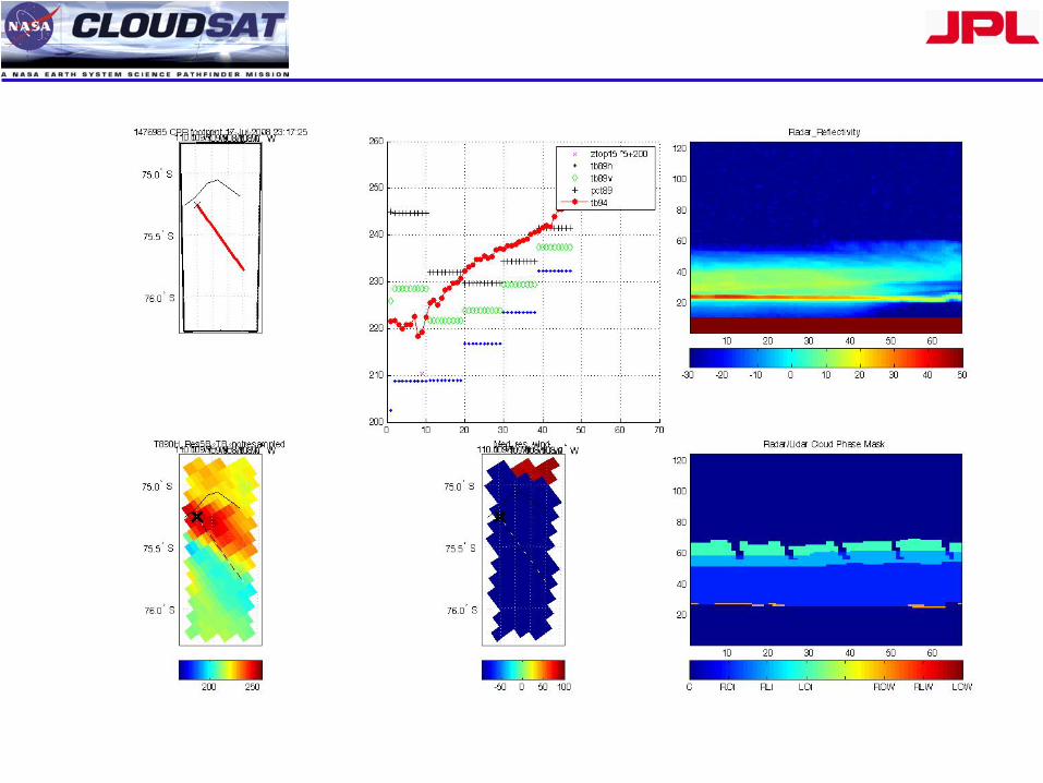
17 July 2008

black marker at ray 30, white at ray 60

22

23

24

25

26

Summary

• CPR is not a youngster anymore but still running strong• Tb will be added to R05. This is an experimental product, feedback from

STM is NECESSARY.