Cloud Filtering Methodology for the Use of Optical Satellite Images in Sustainable 

Management of Tea Plantations

Dr. Ranjith Premalal De SilvaHead, Department of Agricultural Engineering University of PeradeniyaSRI LANKA.

Introduction

9% of World production share & 19% of global export demand are fulfilled by Ceylon Tea

Remote sensing can be used for estimating area of cultivationpredicting yieldidentifying areas affected by pests & diseases and drought

Introduction contd.

There is no effective non destructive method to determine biomass of tea Field measurements are time and labourconsuming and costlyDetection of temporal variation is almost impossible and not very accurate. Remote sensing is an effective method to overcome above constraints and it’s the ideal tool to manage large extents of Tea lands.

Introduction contd.

Clouds is one of the significant obstacles in extracting information from tea lands using remote sensing imagery

Hidden  information.

Cloud contaminated pixels give wrong information.

Optical depth & size of  cloud limit the Geo‐statistical 

interpolation.

Spatial complexity of the land cover also limit the Geo‐

statistical interpolation.

Different approaches have been attempted to solve this problem with varying levels of success.

1. Image fusion 2. Maximum value composites (NDVI)3. Cloud removal based on Histogram Matching4. Wavelet regression.

Introduction contd.

Data: Landsat 7(ETM+) raw images (2003 and 2001) Aster

Software: ERDAS Imagine® v. 8.5 (Leica Geosystems, 2003)GS+ Gama Geo-statistical softwareMicrosoft Excel, ArcGIS

Internet resources.

Resources

Methodology1) Pre-processing

Data Acquisition Importing imagesImage to image registrationSubset images

2) ProcessingCloud filteringFilling out missing information

3) Validation

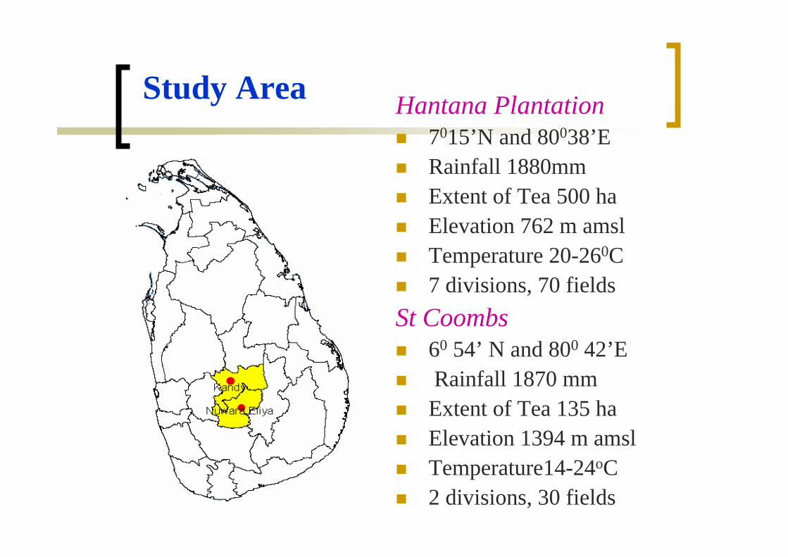
Study Area Hantana Plantation7015’N and 80038’E Rainfall 1880mm Extent of Tea 500 haElevation 762 m amslTemperature 20-260C 7 divisions, 70 fields

St Coombs60 54’ N and 800 42’ERainfall 1870 mmExtent of Tea 135 haElevation 1394 m amslTemperature14-24oC 2 divisions, 30 fields

30m 14.03.2001 HantanaSt Coombs

Landsat

15m 15.01.2003 Hantana Aster

Spatial resolution

Acquisition Date

SiteImage

Satellite images

Step 1 - Cloud Filtering

Pre-processing Processing Validation

Data Acquisition Importing imagesImage to image registrationSubset images

3 Subset Images3 Subset Images

Masked ImagesMasked Images

Thermal ImageThermal Image

Temperature Mapped ImageTemperature

Mapped Image

Subset ImagesSubset Images

Subject ImageSubject Image

Recoded ImageRecoded Image

Pixel to ASCII

SemivariogramSemivariogram KrigingKriging

Multi-spectral ImagesMulti-spectral Images

Image Image

Processing

1) Cloud filtering1.Image calibration2.Threshold3. Masking

2) Filling out missing information1. Method 1‐Geostatistical interpolation2. Method 2‐Regression model

Temperature calculation algorithmInput raster

Output temperature image

Processing (Cloud filtering)

Threshold‐ Identify the pixel range appear as clouds 

and shadow in histogram‐ Recode that pixel range into zero

Masking‐ Select the recoded thermal image as 

input mask‐ Filter out the clouds and shadow area in multispectral images

Processing (Filling out missing information)

‐ Select single cloud patch- Export surrounding pixel value as ASCII file

‐ Semi-variogramsPlot the semivariograminterpolation interval =30fitted with spherical model

Method 1- Filling out gaps using kriging

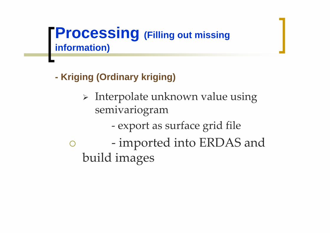
Interpolate unknown value using semivariogram‐ export as surface grid file‐ imported into ERDAS and 

build images

- Kriging (Ordinary kriging)

Processing (Filling out missing information)

Building the regression modelBuild model with co‐located pixels in reference imageSeparated model for each band

Applying  regression modelNew DNs were predicted for each pixel

( )∫= refisubji XY

Method 2 - Filling out gaps using regression model

Processing (Filling out missing information)

ValidationEvaluate those proceduresSelect cloud free part as cloud areapredict the pixel values using kriging and regression model

Compare predicted image part with original imageKriging‐ cross‐validation analysis‐ layer statistic

Regression model ‐absolute differences between pixel values‐ layer statistic

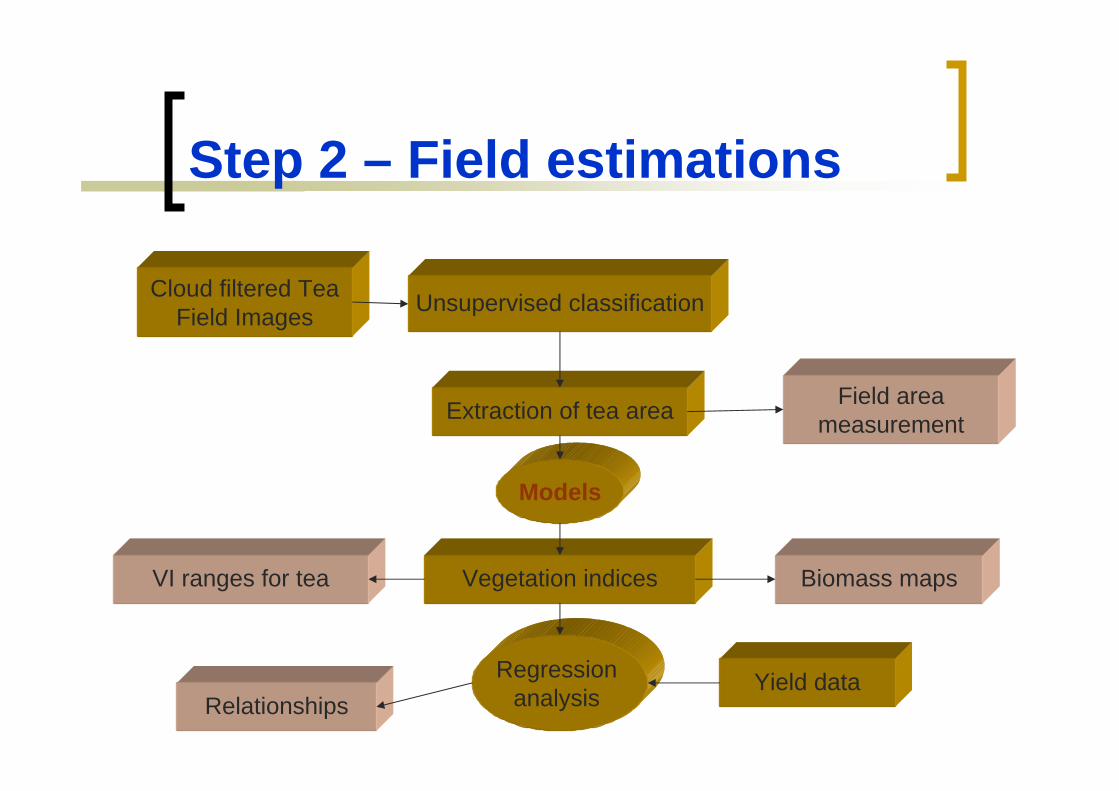
Step 2 – Field estimations

Cloud filtered Tea Field Images

Extraction of tea area

Unsupervised classification

Field area measurement

Vegetation indices Biomass mapsVI ranges for tea

Models

Regression analysis

Yield dataRelationships

Modeler Modelmaker

NDVIDVIRVI

NIR - RedNIR + Red

NDVI =

DVI = NIR - Red

=RVI NIRRed

Results

high sensitivity to cloud areas and it can clearly identify dense cloud as well as thin cloudsNo confusion with other ground objectsshadow detection performs better 

Cloud filtering by thermal band

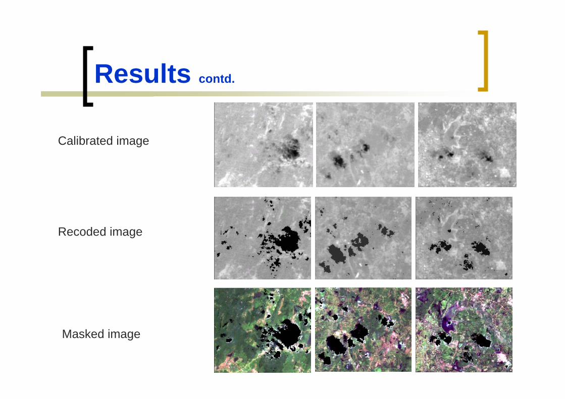
Calibrated image

Recoded image

Masked image

Results contd.

Band 2Band 1 Band 3

Results contd.

Filling out gaps using Kriging

Results contd.

Filling out gaps using KrigingWhite ring surround the cloud patch confuse the kriging process 

Before After

Filling out gaps using regression modelRegression models for each bands (LandSat)

Results contd.

0.452Ysubi = 35.38 + 0.1234 XrefiBand 3

0.234Ysubi = 53.68 + 0.0531 XrefiBand 2

0.768Ysubi = 270.8 ‐ 2.367 XrefiBand 1

Regression coefficient

ModelBand

Filling out gaps using regression model

Results contd.

Band 1 Band 2 Band 3

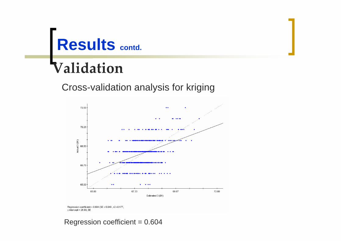
ValidationCross-validation analysis for kriging

Results contd.

Regression coefficient = 0.604

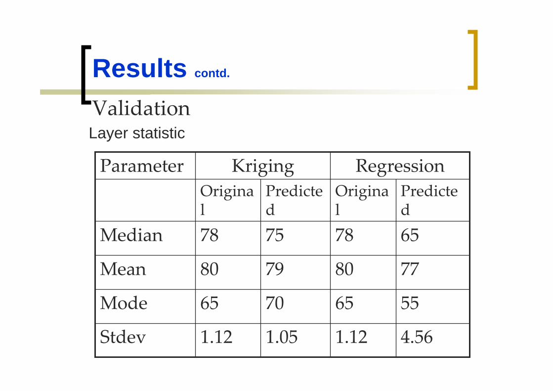
ValidationLayer statistic

55657065Mode

4.561.121.051.12Stdev

80

78

Original

80

78

Original

7779Mean

6575Median

Predicted

Predicted

RegressionKrigingParameter

Results contd.

Results contd.

Area Extraction

Hantana plantations FCC are important to identify areasUseful for change detection

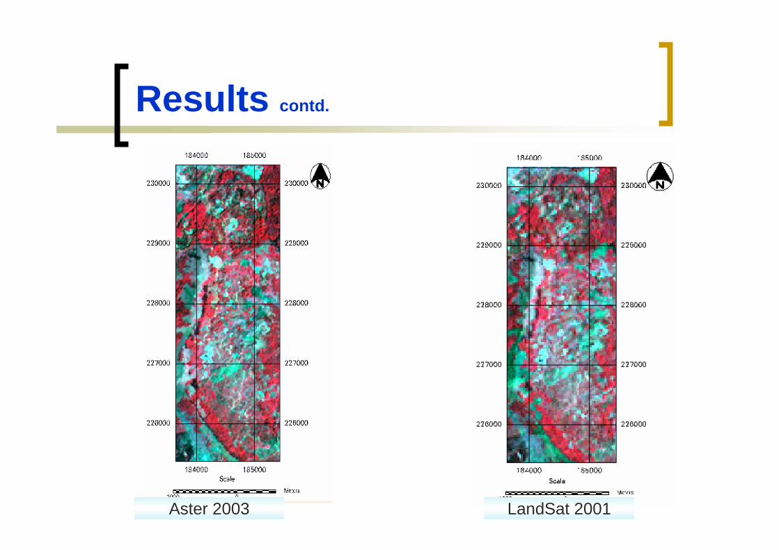
Aster 2003 LandSat 2001

Results contd.

NDVI

Aster 2003 LandSat 2001

DVI

Aster 2003 LandSat 2001

RVI

Aster 2003 LandSat 2001

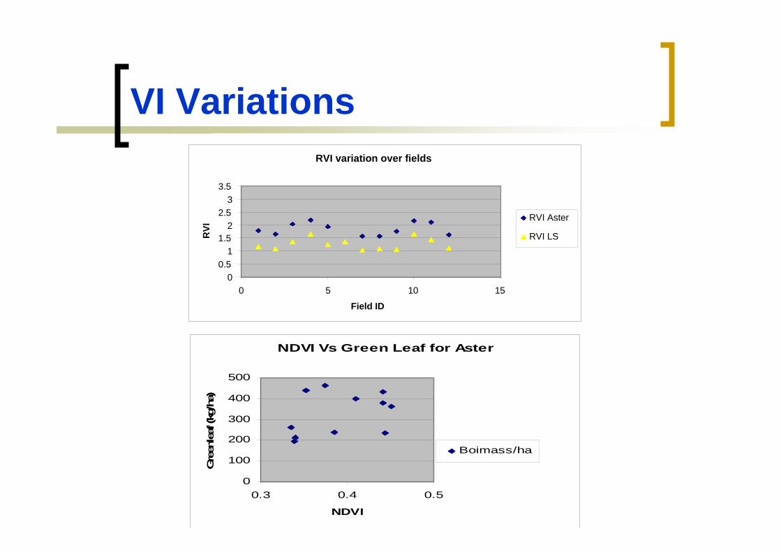
VI Variations

NDVI Vs Green Leaf for Aster

0

100

200

300

400

500

0.3 0.4 0.5

NDVI

Gre

enle

af (k

g/ha

)

Boimass/ha

RVI variation over fields

00.5

11.5

22.5

33.5

0 5 10 15

Field ID

RVI

RVI Aster

RVI LS

0.19530.1968

0.0873 0.0111

RVI

0.18330.1826

0.0687 0.0033

DVI

0.19010.1903

0.1224 0.0179

NDVI

LANDSATASTERR2

NDVI – DVI

St Coombs estate Thalawakele

Landsat 2001

NDVI

Landsat 2001

DVI

Landsat 2001

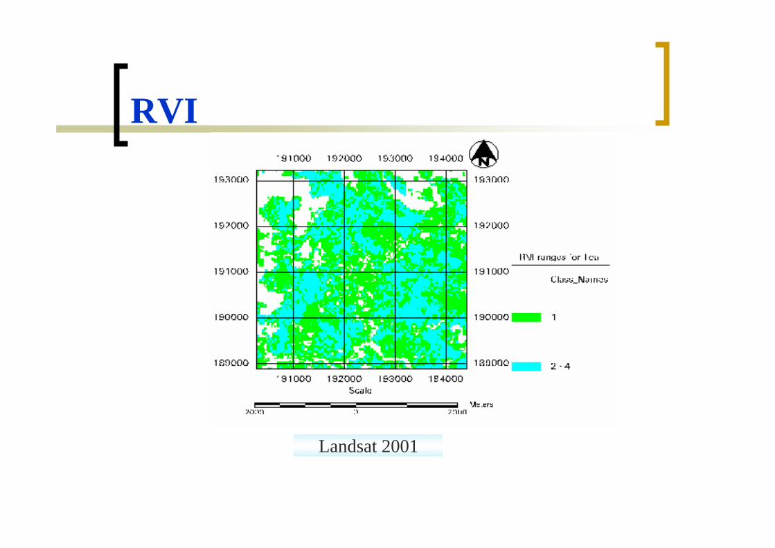
RVI

Landsat 2001

Conclusions

Thermal band detected the clouds and shadow precisely. It does not confuse with other ground objects as cloud. Thermal band can detect large clouds as well as thin cloudsKriging for filling out cloud area perform better and low spatial complexity under cloud area.Regression model does not perform better than kriging method for filling out missing information caused by cloud and shadow 

ConclusionsNDVI and DVI show similar representations of tea biomass. Variation of biomass of tea is reflected in different categories in NDVI, DVI and RVI maps.There’s no significant correlation between vegetation indices and tea yields / plucked green leaf.It was not possible to identify any effect of spatial resolution on determining these relationships.Higher the spatial resolution narrower the range for vegetation indices.

In Thalawakale the biomass cover is not changed very much in 1992,1998, 2001. Up country tea gives higher VI values than mid country representing dense cover of vegetation.

Conclusions

Thank You