Closed-Loop Control of Ankle Plantarflexors and ... · ii Closed-loop control of ankle...
190
Closed-Loop Control of Ankle Plantarflexors and Dorsiflexors using an Inverted Pendulum Apparatus by Michael Same A thesis submitted in conformity with the requirements for the degree of Master of Applied Science Institute of Biomaterials and Biomedical Engineering University of Toronto © Copyright by Michael Same 2014
Transcript of Closed-Loop Control of Ankle Plantarflexors and ... · ii Closed-loop control of ankle...
Closed-Loop Control of Ankle Plantarflexors and
Dorsiflexors using an Inverted Pendulum Apparatus
by
Michael Same
A thesis submitted in conformity with the requirements for the degree of Master of Applied Science
Institute of Biomaterials and Biomedical Engineering University of Toronto
© Copyright by Michael Same 2014

ii
Closed-loop control of ankle plantarflexors and dorsiflexors using
an inverted pendulum apparatus
Michael Same
Master of Applied Science
Institute of Biomaterials and Biomedical Engineering
University of Toronto
2014
Abstract
In the past, it has been shown that functional electrical stimulation (FES), when applied to lower
limbs, can facilitate quiet stance in patients with various neurological disorders. Furthermore, the
literature suggests that able-bodied individuals regulate balance during quiet stance using a
control strategy that is similar to proportional-integral-derivative (PID) control. The purpose of
this study was to test if a PID control strategy is capable of effectively regulating an FES system
at the ankle joints during quiet stance. Specifically, we tested whether able-bodied individuals
with compromised visual, vestibular and proprioceptive senses, would exhibit improved ankle
joint control if FES was applied to contract the ankle muscles using a closed-loop, PID control
strategy. In what follows we show that the proposed PID control strategy was able to outperform
voluntary control of the ankle joint, indicating that the controller could be considered for use in
neurological patients, including spinal cord injured individuals.

iii
Acknowledgments
First and foremost, I would like to sincerely thank Dr. Milos Popovic for his supervision,
inspiration and guidance throughout my masters. From the outset, his enthusiasm and passion for
the project was truly contagious. He always gave me the freedom to learn and grow
independently, encouraging me to reach my potential, but was also always available to provide
first-rate advice and feedback.
I would also like to thank various members of the Rehabilitation Engineering Laboratory (REL)
for always being so happy and willing to provide their expertise and offer their assistance. Dr.
Hossein Rouhani, in particular, was an incredible mentor, who always made himself available,
even on weekends and evenings, to offer useful, friendly guidance and feedback (and to provide
some ankle muscles for testing). Similarly, in addition to the input and guidance that he gave me
in his role as a member of my thesis committee, Dr. Kei Masani was always available to review
documents, address queries, and provide expert guidance. The advice and assistance of Dr. Paul
Yoo, the other member of my thesis committee, was also greatly appreciated. The tireless efforts
of Mr. Adolazim Rashidi to assist with the development of multiple mechanical and electrical
devices were also indispensible. I’d also like to thank all of my subjects for selflessly giving of
their time and their leg muscles. Finally, I want to acknowledge the REL team as a whole, and
the B4 folks in particular, for their support and their help in creating an enjoyable, productive
environment for performing meaningful research.
Finally, the support and encouragement provided by family and friends over the duration of my
masters has been exemplary and was fundamental in me achieving my goals. In particular, to my
family, even though the distances between us are rather large these days, your continued support
means everything to me.

iv
Table of Contents
Chapter 1 Introduction ................................................................................................................ 1
1 Introduction ........................................................................................................................... 1
1.1 Motivation ...................................................................................................................... 1
1.2 Organization of Thesis .................................................................................................... 2
Chapter 2 Literature Review ....................................................................................................... 3
2 Literature Review .................................................................................................................. 3
2.1 Physiology of Able-Bodied Stance .................................................................................. 3
2.2 Functional Electrical Stimulation (FES) .......................................................................... 5
2.3 FES for Standing............................................................................................................. 6
2.3.1 Open-loop Control............................................................................................... 8
2.3.2 PID / PD Control Strategies ................................................................................. 9
2.3.3 Other Control Strategies .................................................................................... 10
Chapter 3 Research Questions and Hypotheses ......................................................................... 13
3 Research Questions and Hypotheses .................................................................................... 13
3.1 Research Questions ....................................................................................................... 13
3.2 Thesis Objectives .......................................................................................................... 14
3.3 Hypotheses ................................................................................................................... 14
Chapter 4 Methods ................................................................................................................... 16
4 Methods ............................................................................................................................... 16
4.1 Overview ...................................................................................................................... 16
4.2 Equipment .................................................................................................................... 16
4.2.1 The Inverted Pendulum Standing Apparatus ...................................................... 16
4.2.2 Other components ............................................................................................. 23
4.3 PID plus Gravity Control Strategies .............................................................................. 25
4.3.1 Overview........................................................................................................... 25

v
4.3.2 PID plus Gravity Controllers Outputting Required Torque (Controller A) ......... 25
4.3.3 PID plus Gravity Controllers Outputting Required FES Current (Controller B) . 31
4.4 Simulations ................................................................................................................... 37
4.4.1 Simulations using Controller A.......................................................................... 37
4.4.2 Simulations using Controller B .......................................................................... 40
4.5 Experimentation in Able-Bodied Subjects ..................................................................... 47
4.5.1 Initial setup ....................................................................................................... 47
4.5.2 Experiment 1: Preliminary experiments in 3 subjects (Controller A) .................. 49
4.5.3 Experiment 2: Experiments in 11 subjects (Controller B) .................................. 53
4.5.4 Experiment 3: Experiments in 3 subjects (Variant of Controller B) .................... 57
4.5.5 Data Analysis .................................................................................................... 57
Chapter 5 Results ..................................................................................................................... 60
5 Results ................................................................................................................................. 60
5.1 Overview ...................................................................................................................... 60
5.2 Subjects ........................................................................................................................ 60
5.3 Experiment 1 ................................................................................................................ 62
5.3.1 Calibration ........................................................................................................ 62
5.3.2 Experimental Trials ........................................................................................... 62
5.3.3 Simulations ....................................................................................................... 67
5.4 Experiment 2 ................................................................................................................ 70
5.4.1 Calibration ........................................................................................................ 70
5.4.2 Establishing Controller Parameters .................................................................... 77
5.4.3 Quiet Standing................................................................................................... 83
5.4.4 Step Responses .................................................................................................. 91
5.4.5 External Perturbations ......................................................................................103
5.4.6 Body Weight Matching ....................................................................................106

vi
5.4.7 Correlations ......................................................................................................114
5.4.8 Tests of Stability ..............................................................................................114
5.5 Experiment 3 and Comparisons between Experiments .................................................117
5.5.1 Experiment 3 Calibration, Simulations and Fine-Tuning ...................................117
5.5.2 Quiet Standing Trials ........................................................................................119
5.5.3 Step Response Trials ........................................................................................123
5.5.4 Perturbation Trials ............................................................................................127
5.5.5 Body Weight Matching ....................................................................................129
5.5.6 Fatigue Tests ....................................................................................................133
5.5.7 Stability Tests ...................................................................................................134
Chapter 6 Discussion ...............................................................................................................137
6 Discussion ..........................................................................................................................137
6.1 Overview .....................................................................................................................137
6.2 Experimental Results ...................................................................................................137
6.2.1 Voluntary Conditions with Eyes Open/Closed ..................................................137
6.2.2 Trials with the FES Controller ..........................................................................139
6.3 Simulation Results .......................................................................................................147
6.4 Limitations and Future Directions ................................................................................149
6.4.1 Performing experiments in more able-bodied subjects ......................................149
6.4.2 Investigating alternative calibration procedures ................................................150
6.4.3 Performing similar experiments in patient populations......................................151
6.4.4 Examining methods of better modelling stance in paraplegic or other patient
populations using the IPSA ..............................................................................151
6.4.5 Testing controller performance in the presence of substantial measurement
noise.................................................................................................................152
6.4.6 Expanding the Simulink models to incorporate patient populations ..................152
6.4.7 Altering the controller design to minimize “integrator windup” ........................153

vii
6.4.8 Expanding the control system to include other degrees of freedom ...................153
6.4.9 Examining other, more complex controller types ..............................................154
Chapter 7 Conclusion ..............................................................................................................155
7 Conclusion ..........................................................................................................................155

viii
List of Tables
Table 5.1: Anthropometric data for each subject. ...................................................................... 61
Table 5.2: Controller gains employed in Experiment 1. ............................................................ 63
Table 5.3: Experiment 1 performance measures. ....................................................................... 64
Table 5.4: Controller gains that minimized root mean square error (RMSE) in Experiment 1
simulations. .............................................................................................................................. 69
Table 5.5: First order muscle recruitment dynamics model parameters for Experiment 2. ......... 76
Table 5.6: Controller gains suggested from simulations and employed in Experiment 2. ........... 80
Table 5.7: Performance measures for Experiment 2 quiet standing trials. .................................. 85
Table 5.8: Performance measures for Experiment 2 step response trials. ................................... 97
Table 5.9: Step response performance meausres for Experiment 2 step response trials. ........... 100
Table 5.10: Performance measures for Experiment 2 external perturbation trials. ................... 105
Table 5.11: Summary of body weight matching parameters .................................................... 107
Table 5.12: Performance measures for Experiment 2 body weight matched step response trials.
............................................................................................................................................... 111
Table 5.13: Step response performance measures for Experiment 2 body weight matched step
response trials. ........................................................................................................................ 112
Table 5.14: First order muscle recruitment dynamics model parameters for Experiment 3. ..... 117
Table 5.15: Controller gains suggested from simulations and employed in Experiment 3. ....... 118
Table 5.16: Comparison of performance measures obtained in quiet standing trials in
Experiments 1-3. .................................................................................................................... 122
Table 5.17: Comparison of performance measures obtained in step response trials in Experiments

ix
2 and 3. .................................................................................................................................. 125
Table 5.18: Comparison of performance measures obtained during steps in step response trials in
Experiments 2 and 3. .............................................................................................................. 126
Table 5.19: Comparison of performance measures obtained in external perturbation trials in
Experiments 2 and 3. .............................................................................................................. 129

x
List of Figures
Figure 2.1: A typical FES waveform ........................................................................................... 5
Figure 2.2: A model of the 12 physiologically realizable degrees of freedom in the lower limbs . 7
Figure 4.1: Inverted Pendulum Standing Apparatus (IPSA) ...................................................... 18
Figure 4.2: Subject standing in the Inverted Pendulum Standing Apparatus (IPSA) .................. 19
Figure 4.3: Diagram depicting a subject’s feet attached to the foot plates .................................. 21
Figure 4.4: The perturbation bar used to apply external perturbations to the inverted pendulum 25
Figure 4.5: Block diagram depicting the first PID plus gravity control strategy (Controller A) .. 26
Figure 4.6: PID controller configuration employed in Experiments 1-3 ..................................... 27
Figure 4.7: Muscle recruitment curves for (a) plantarflexors and (b) dorsiflexors, for use with
Controller A ............................................................................................................................. 30
Figure 4.8: Block diagram depicting the second PID plus gravity control strategy (Controller B)
................................................................................................................................................. 31
Figure 4.9: Calibration curves used for defining the muscle dynamics of the plantarflexors in
Controller B ............................................................................................................................. 35
Figure 4.10: Calibration curves used for defining the muscle dynamics of the dorsiflexors in
Controller B ............................................................................................................................. 36
Figure 4.11: Bode plots of phase and amplitude response data .................................................. 37
Figure 4.12: Simulink model used for simulating system behaviour with Controller A ............. 39
Figure 4.13: Simulink model used for simulating system behaviour for Experiment 2 using
Controller B ............................................................................................................................. 42
Figure 4.14: Simulink model for Controller B including adjustments made post-experimentation

xi
................................................................................................................................................. 46
Figure 4.15: Approximate FES electrode placements ................................................................ 48
Figure 4.16: An example of the visual feedback available during a Voluntary Condition with
Eyes Open trial ......................................................................................................................... 57
Figure 5.1: Muscle recruitment curves of Subjects B and C in Experiment 1............................. 62
Figure 5.2: 10-minute quiet standing trials in Experiment 1 ...................................................... 63
Figure 5.3: Enlarged view of the inverted pendulum angles during the initial 12 seconds of the
10-minute quiet standing trials in Figure 5.2 ............................................................................. 64
Figure 5.4: 1-minute trials in which 4 posterior perturbations were applied in Experiment 1 ..... 65
Figure 5.5: Top: 15 seconds of the 10-minute quiet standing trial in Figure 5.2 for Subject 1 (FES
Condition). Bottom: The corresponding plantarflexor and dorsiflexor currents, and requested
plantarflexor and dorsiflexor torques. ....................................................................................... 66
Figure 5.6: 12-second FES Condition trial in Subject A with the same controller parameters used
in Subjects B and C in Experiment 1 ........................................................................................ 67
Figure 5.7: Enlarged view of the initial 8 seconds of the 10-minute quiet standing trials shown in
Figure 5.2, comparing the results of experiments simulations using the same controller
parameters ................................................................................................................................ 68
Figure 5.8: Simulation of inverted pendulum angle (in blue) for Subject 1 at the controller
parameters that minimized RMSE ............................................................................................ 68
Figure 5.9: Bode plots based on simulations at the controller parameters employed in Experiment
1 ............................................................................................................................................... 69
Figure 5.10: Bode plots depicting phase and amplitude response data in Experiment 2. ............ 75
Figure 5.11: Step response curves obtained experimentally (black) and based on first order
muscle dynamics models (blue) for Subject 1 in Experiment 2 ................................................. 77

xii
Figure 5.12: The beginning of an Experiment 2 FES Condition trial in Subject 8. ..................... 82
Figure 5.13: The beginning of an Experiment 2 FES Condition trial in Subject 9 ...................... 83
Figure 5.14: 5-minute quiet standing trials in Experiment 2 ...................................................... 84
Figure 5.15: Enlarged views of a 30-second period beginning after 150 seconds of the 5-minute
quiet standing trials in Experiment 2 ......................................................................................... 87
Figure 5.16: Enlarged views of periods during the 5-minute quiet standing trials in 5 subjects in
which the required FES current applied to the plantarflexors to maintain the inverted pendulum
against gravity decreased over time. ......................................................................................... 89
Figure 5.17: The initial 14 seconds of the 5-minute quiet standing trials in Experiment 2. ........ 90
Figure 5.18: Step response trials for Subject 1 in Experiment 2................................................. 91
Figure 5.19: Step response trials for Subject 2 in Experiment 2................................................. 92
Figure 5.20: Step response trials for Subject 3 in Experiment 2................................................. 92
Figure 5.21: Step response trials for Subject 4 in Experiment 2................................................. 93
Figure 5.22: Step response trials for Subject 5 in Experiment 2................................................. 93
Figure 5.23: Step response trials for Subject 6 in Experiment 2................................................. 93
Figure 5.24: Step response trials for Subject 7 in Experiment 2................................................. 94
Figure 5.25: Step response trials for Subject 8 in Experiment 2................................................. 94
Figure 5.26: Step response trial in Subject 8 under the FES Condition. The real-time inverted
pendulum angle (blue) is shown, as well as the plantarflexor (grey) and dorsiflexor (green)
currents. ................................................................................................................................... 95
Figure 5.27: 90-second step response trials (FES Condition) testing the effect of increasing or
decreasing the proportional, derivative and/or integral gains by 30% in Subject 1 in Experiment
2. ............................................................................................................................................ 102

xiii
Figure 5.28: External perturbation trials in Experiment 2 ........................................................ 104
Figure 5.29: Step response trials in the body weight matching paradigm for Subject 1 and 5 in
Experiment 2 .......................................................................................................................... 108
Figure 5.30: Step response trials in the body weight matching paradigm for Subject 3 and 4 in
Experiment 2. ......................................................................................................................... 109
Figure 5.31: Inverted pendulum angle and plantarflexor current amplitude during a 10-minute
quiet standing trial in Subject 1 with body weight matching (FES Condition) ......................... 113
Figure 5.32: Bode plots depicting gain and phase margins for Subjects 1-7............................. 115
Figure 5.33: Bode plots depicting gain and phase margins in the body weight matching
paradigm. ............................................................................................................................... 116
Figure 5.34: Comparison of 5-minute quiet standing trials (FES Condition) across the 3
experiments in Subjects A1i and C2ii.. ................................................................................... 119
Figure 5.35: 5-minute quiet standing trials for Subject iii in Experiment 3 .............................. 120
Figure 5.36: Enlarged view of the beginnings of the trials depicted in Figure 5.34. ................. 121
Figure 5.37: Enlarged views of the trials depicted in Figure 5.35 for Subject iii in Experiment 3
............................................................................................................................................... 121
Figure 5.38: Comparison of step response trials for Subject A1i in Experiments 2 and 3......... 123
Figure 5.39: Comparison of step response trials for Subject C2ii in Experiments 2 and 3 ........ 124
Figure 5.40: Step response trials for Subject iii in Experiment 3. ............................................ 124
Figure 5.41: Comparison of external perturbation trials (FES Condition) for Subjects A1i and
C2ii in Experiments 2 and 3.................................................................................................... 128
Figure 5.42: External perturbation trial for Subject iii in Experiment 3 ................................... 128
Figure 5.43: Comparison of step response trials in the body weight matching paradigm for

xiv
Subject A1i in Experiments 2 and 3 ........................................................................................ 130
Figure 5.44: Step response trials in the body weight matching paradigm for Subject C2ii in
Experiment 3. ......................................................................................................................... 131
Figure 5.45: Tests of fatigue ................................................................................................... 133
Figure 5.46: Bode plots depicting gain and phase margins in Subjects i, ii and iii in Experiment
3. ............................................................................................................................................ 134
Figure 5.47: Bode plots depicting gain and phase margins in the body weight matching paradigm
for Subjects i and ii in Experiment 3. ...................................................................................... 135
Figure 5.48: Colour maps depicting gain margins and phase margins for varying proportional and
derivative gains ...................................................................................................................... 136

xv
List of Appendices
A APPENDIX A: Simulink submodules 167
B APPENDIX B: Experiment 2 calibration curves
168

1
Chapter 1
Introduction
1 Introduction
1.1 Motivation
In Canada alone, an estimated 86,000 individuals are currently living with a spinal cord injury
(SCI), and approximately 4,000 new cases are reported each year1. All SCI patients suffer from a
diminished ability or complete inability to maintain balance during quiet stance due to deficits in
neuromuscular function2. Other conditions such as stroke
3 and traumatic brain injury (TBI)
4 can
also lead to impaired standing ability. Significant demand exists for techniques aimed at enabling
stable stance in these populations as a means of improving quality of life and independence, as
well as encouraging exercise of paralyzed or paretic muscles so as to minimise the likelihood of
secondary complications arising from confinement to a wheelchair, such as osteoporosis5,
urinary tract infections6, spasticity
7, pressure ulcers
8 and cardiovascular disease
9. Facilitating
stance without the requirement for upper limb support would be particularly advantageous as
patients would then be free to use their hands to perform activities of daily living while standing.
The application of functional electrical stimulation (FES) for the attainment of this goal has
attracted considerable interest over the past 30 years. FES refers to patterned electrical
stimulation of paralyzed or paretic muscles to induce contractions and generate limb or body
movements. In clinical conditions such as SCI where there exists an impaired ability to generate
or transmit motor commands to certain muscles, FES systems termed neuroprostheses can be
used to replace to some extent the functionality of the central nervous system in controlling the
muscles10,11
.
A standing neuroprosthesis could potentially overcome multiple limitations of mechanical
solutions for facilitating stance, such as mechanical orthoses or standing frames. First,
mechanical systems are bulky and heavy, difficult to don and doff and not cosmetically
appealing, thus limiting usability, particularly in home settings12-14
. Second, orthoses and
standing frames typically require upper limb support, unnatural stance postures and/or control of
the upper body to maintain stability, thus limiting the potential for performing activities of daily
living while standing12,15
. Third, active standing, achieved via FES-induced muscle contractions,

2
offers more physiological benefits than the passive standing which is facilitated by mechanical
devices. In particular, FES-assisted stance has been found to increase blood flow, improve
muscle tissue health, and increase bone density; thus minimising the likelihood of developing
cardiovascular disease, spasticity or pressure ulcers, or osteoporosis, respectively16-21
. Finally,
active standing using FES could potentially be employed therapeutically to retrain muscle
control and improve standing ability in incomplete SCI patients and other neurologic patients22
.
Despite the potential benefits of FES-assisted stance, the clinical applicability of current and
previously developed standing neuroprostheses remains limited. In particular, the goal of hands-
free paraplegic stance, without the requirement for bracing of multiple joints, remains unfulfilled.
Although there are multiple technological challenges that stand in the way of developing a
hands-free neuroprosthesis for standing, probably the most difficult of them all is the
development of a closed-loop control strategy that will allow one to adequately and reliably
control FES during stance in response to internal perturbations (such as muscle fatigue, spasms,
etc.) and external perturbations. This thesis presents and validates a closed-loop control strategy
for modulating FES levels applied to the ankle muscles during quiet stance. It is hoped that this
research could potentially act as a first step towards the development of a clinically relevant
standing neuroprosthesis to improve or restore standing ability in neurologic patient populations.
1.2 Organization of Thesis
This thesis is comprised of seven chapters. Chapter 2 presents a literature review, focusing on
both the physiological control strategy employed in able-bodied stance, and artificial control
strategies that have been investigated for modulating FES levels applied to the lower limbs to
improve standing ability. In Chapter 3, thesis objectives and hypotheses are presented. In
Chapter 4, the methodology is discussed, including descriptions of the experimental setup, the
control strategy, and the procedures for evaluating the performance of the control strategy
through simulations and experiments in able-bodied subjects. The results of these simulations
and experiments are presented in Chapter 5, and analyzed in the Discussion in Chapter 6.
Chapter 6 also examines the significance of the findings, discusses limitations of the protocol,
and highlights recommended future work to expand upon this research and ultimately move
towards clinical applicability. Finally, Conclusions are presented in Chapter 7.

3
Chapter 2
Literature Review
2 Literature Review
This chapter reviews the research that has been conducted towards the development of a
neuroprosthesis for standing. In particular, different approaches to controlling movement in the
ankle joint during stance are presented. In Section 2.1, control strategies employed by the central
nervous system in able-bodied stance, particularly at the ankle joint, are discussed. Section 2.2
provides some brief background into FES. Finally, Section 2.3 discusses various control
strategies that have been employed to modulate FES levels applied to muscles of the lower limbs
and particularly the ankle muscles, for the ultimate purpose of developing a clinically applicable
standing neuroprosthesis.
2.1 Physiology of Able-Bodied Stance
The control mechanisms employed to maintain balance during able-bodied stance have been
extensively studied. In particular, control of movement in the anterior/posterior (A/P) direction
(i.e., in the sagittal plane) about the ankle joint has been widely investigated. This is because the
ankle joints have been found to be the dominant joints for maintaining balance during quiet
stance, as evidenced by the fact that able-bodied stance has been effectively modelled in multiple
studies as an inverted pendulum rotating about the ankle joints23-25
. This inverted pendulum
model has been found to fit well with experimental data obtained during quiet standing trials23-25
.
Based on this model, control of the ankle joints in able-bodied stance can be considered to
consist of mechanisms for regulating ankle torque to maintain the centre of mass about an
equilibrium position, and to compensate for the effects of gravity. This regulation of ankle torque
is achieved both passively, due to the intrinsic mechanical properties of the lower limbs
(modeled as a mass-spring-damper system acting around the ankle joint), and actively, through
muscle contractions regulated by the central nervous system (CNS) based on feedback
information received from the sensory systems. Whilst the relative contributions of these two
components is disputed, it is known that passive contributions alone are insufficient for
maintaining stability and that some active control of stance is required26
.

4
The nature of the control strategy employed by the CNS is also the subject of some conjecture,
with some groups hypothesizing the presence of a predictive, feed-forward mechanism25,27
and
others suggesting that a feedback mechanism is responsible28-31
. Previous studies have shown
that muscle activity in the plantarflexors correlates with and temporally precedes A/P
displacements of the centre of mass (COM)25,28
, thus implying the existence of some mechanism
for modulating muscle activity in anticipation of fluctuations in COM, which is a key tenet in the
argument for the presence of a feed-forward mechanism. However, studies performed by our
group and others have suggested that a feedback mechanism based largely on changes in the
COM velocity could be responsible for this modulation28-31
. In other words, it has been
established by our laboratory and others that a feed-forward mechanism is not necessary to
maintain stability, and that a feedback mechanism based largely on displacement and velocity
information can predict experimental results and theoretically stabilize the body in spite of large
neural and torque generation delays.
For example, in a study performed by our group, cross-correlation analyses performed on
experimental able-bodied quiet standing data established that changes in COM velocity reliably
precede (by approximately 120 ms) variations in plantarflexor activation28
. Moreover, the
presence of a feedback system based on fluctuations in COM displacement, velocity and
acceleration for other muscle groups actuating the ankles, knees, hips and trunk, has also been
suggested, with the model accounting for over 67% of EMG variability31
.
Multiple studies have also compared physiological control strategies to proportional-derivative
(PD) or proportional-integral-derivative (PID) controllers29,30,32-35
. These control structures
include a proportional component which varies proportionally with displacement, and a
derivative component which varies proportionally with velocity (see Section 3.3.2 for more
details). Thus, by employing COM as the process variable (i.e., the variable to be controlled), PD
and PID controllers factor in the apparent importance of COM displacement and velocity
information. In multiple studies, PD and PID controllers have been used to model the neural
control component of able-bodied stance and have been shown to fit very well with physiological
control strategies29,30,32,33,36
. Using these models of neural control, in combination with passive
standing components, experimental results have been successfully and reliably predicted30,32,33,36
.
Similarly, simulations have suggested that a PD or PID-type control strategy could successfully
stabilize the body during quiet and perturbed stance29,34-36
, despite modelled neurological and

5
torque generation delays of up to 200 - 380 ms36
. Although the actual magnitudes of these delays
are the subjects of some conjecture, values of 200 – 380 ms are at the higher end of total delay
values typically quoted in the literature29,32,36-38
.
In this study, a similar control strategy was implemented to attempt to mimic the physiological
control strategy for standing by regulating levels of functional electrical stimulation (FES)
applied to the ankle muscles. Section 2.3.2 discusses some results of preliminary studies utilizing
PD and PID control strategies in combination with FES.
2.2 Functional Electrical Stimulation (FES)
Applying electrical pulses through stimulating electrodes to the nerves innervating muscles can
induce localized electric fields, resulting in cell membrane depolarization. At appropriate
stimulation parameters, action potentials are induced which can propagate across the
neuromuscular junction, resulting in the contraction of muscle fibres11
. The patterned electrical
stimulation of muscles to induce contractions and generate movements is termed functional
electrical stimulation (FES). Figure 2.1, below, depicts a typical FES waveform. Note that three
distinct parameters (current amplitude, frequency, and pulse duration) can be adjusted to vary the
effects on the muscle tissue.
Figure 2.1: A typical FES waveform
In the past 50 years, considerable research has been conducted into potential applications of FES
for restoring function in patients with neuromuscular disorders such as SCI, stroke and traumatic
brain injury. In these and other conditions, where the injury is limited to the upper motor neuron,
and where lower motor neurons are intact, one can generate action potentials in the lower motor
neurons which then can cause muscles that are connected to these neurons to contract. In such
cases, FES systems, termed neuroprostheses, are being developed to replace to some extent the
amplitude
frequency -1
pulse duration

6
functionality of the CNS in controlling the muscles10,11
in order to assist with tasks such as
walking39
, grasping40
, bladder voiding41
or standing42
.
FES can be applied: (1) transcutaneously through surface electrodes that are placed on the skin
above the muscles of interest, (2) percutaneously where electrodes penetrate the skin and are
anchored near or on the nerve that innervates the muscle of interest, or (3) using implanted
electrodes that are surgically placed either on the muscle near the motor junction or on the nerve
that innervates the muscle of interest. Implanted and percutaneous electrodes can offer benefits
over surface technology including enhanced ability to isolate individual muscles and improved
accessibility to deep muscles. However, the invasiveness of the electrode implantation procedure
is a major disadvantage. In contrast, surface electrodes are non-invasive, easy to apply and
remove, inexpensive, and more easily applicable in clinical settings.
2.3 FES for Standing
Considerable research has been carried out towards the development of a neuroprosthesis for
standing. By applying FES to muscles of the trunk and lower limbs, various groups over the past
30 years have attempted to facilitate or improve stance in paraplegics and other relevant
neurological patient populations. Nonetheless, limitations exist with all neuroprostheses
investigated thus far, and as such clinical applicability remains limited.
Ideally, a clinically viable standing neuroprosthesis would combine an overarching control
strategy with a set of either implanted or transcutaneous electrodes applied to various lower limb
muscles to actuate multiple degrees of freedom (DOFs) at the ankle, knee and hip joints. As
shown in Figure 2.2, 12 physiologically feasible DOFs have been established in the lower limbs
(ankle plantarflexion/dorsiflexion; ankle inversion/eversion; knee flexion/extension; hip
flexion/extension; hip abduction/adduction; and hip rotation, all of which act on both left and
right sides)43
. However, simulations performed by our group have suggested that paraplegic
stance could theoretically be maintained by controlling only 6 DOFs34,35
. As shown in Figure 2.2,
these include left and right ankle plantarflexion/dorsiflexion, left and right knee
flexion/extension, hip flexion/extension on one side; and hip abduction/adduction on one side.
Moreover, all of these DOFs have been found to be controllable through muscles that are
accessible with transcutaneous FES. Based on previous FES studies44-47
, the selection of muscles
to be stimulated for effective actuation of these DOFs would likely comprise medial

7
gastrocnemius (ankle plantarflexion, knee flexion), tibialis anterior (ankle dorsiflexion),
quadriceps (knee extension), gluteus maximus and/or semimembranosus (hip extension), and
rectus femoris (hip flexion). However, despite these promising results in simulations, much
research is required before the practical feasibility of such a device can be ascertained.
Figure 2.2: A model of the 12 physiologically realizable degrees of freedom in the lower limbs43
. Simulations
have suggested that control of the 6 degrees of freedom indicated by the red circles would be sufficient for
stabilizing stance34,35
. (Adapted from a figure in Kim et al.’s article34
)
As a first step towards the development of a neuroprosthesis for standing, this thesis focuses on
the development and testing of a technique for controlling plantarflexion and dorsiflexion at the
ankle joint. As discussed in Section 2.1, the ankle joints have been found to be the dominant
joints for control of quiet and mildly perturbed stance in able-bodied individuals. The ankle
joints are also expected to be the most challenging to control since the ankle muscles regulate the
entire body weight at the furthest distance from the COM. Moreover, movement must be
controlled in 2 directions (anterior and posterior), as opposed to some other DOFs which would
predominantly involve controlling movement in only one direction. For example, the knee joints
could likely be controlled effectively by maintaining them in extension. We have also opted to
focus on control of movement in the sagittal (A/P) plane since maintaining stability in this plane
is more challenging than maintaining stability in the medial/lateral (M/L) plane. This is
exemplified by much larger postural sway in the A/P plane than in the M/L plane during able-
bodied stance48
. We propose the implementation of a relatively simple control strategy that
HAT = Head-arms-trunk
HFE = Hip Flexion/Extension
HAA = Hip Abduction/Adduction
KFE = Knee Flexion/Extension
(left & right)
ADP = Ankle dorsiflexion/
plantarflexion (left & right)

8
would more readily facilitate expansion to other DOFs, as well as movement in the M/L plane, in
the near future.
2.3.1 Open-loop Control
Initial (and some ongoing) attempts at developing a standing neuroprosthesis utilized open-loop
control strategies, in which various muscles were stimulated continuously at constant stimulation
levels (i.e., constant stimulation parameters). Beginning in the late 1970s through the pioneering
work of Alojz Kralj and his group49,50
, these methods have proven capable of facilitating stance
in paraplegic patients. In particular, by transcutaneously stimulating different sets of muscles
actuating the knee and hip joints, Kralj et al.50
were able to automatically switch between
multiple distinct standing postures in paraplegic subjects. As a result, the rate of fatigue of any
one muscle was diminished and, with the incorporation of upper limb support, standing durations
of up to 5 hours were obtained. The development of FES paradigms for restrengthening
atrophied muscles in the weeks prior to experimentation also assisted in facilitating these results
by delaying the onset of fatigue51
. More recently, research undertaken by Ronald Triolo’s group
has focused on the development and testing of 8-channel52
and 16-channel53
implanted FES
systems for stimulating various lower limb muscles and nerves in open-loop and facilitating
stance. These neuroprostheses have been implanted in approximately 20 paraplegic patients thus
far and have facilitated stance for up to 2 hours with up to 95% of body weight supported by the
lower limbs, although a marked drop in performance has been observed with taller and heavier
subjects.
Despite these promising results, all previously developed open-loop controlled neuroprostheses
suffer a key limitation. Since open-loop FES systems contract muscles continuously and are not
designed to provide stabilization, users are required to stabilize themselves by holding a walker
or a frame during standing. In addition, these continuous muscle contractions result in rapid
muscle fatigue. The user must then compensate for this muscle fatigue in the lower limbs by
providing increased upper limb and trunk strength. Following many tests with patients it has
become evident that in order for a neuroprosthesis for standing to have any clinical value it must
enable stable standing, where the user will have both of their arms free (hands-free standing) to
perform bimanual tasks while standing. To achieve this, a neuroprosthesis for standing must be
able to regulate balance autonomously (i.e., in a closed-loop configuration). Therefore, a closed-

9
loop feedback controller, which is able to vary the intensity of stimulation applied to different
muscles of the lower limbs in order to compensate for disturbances and fluctuations in balance, is
required. Such a control system would also offer the advantage of not providing stimulation
when muscles do not need to be contracted, which would in turn minimize fatigue.
2.3.2 PID / PD Control Strategies
As was discussed in Section 2.1, PID or PD control strategies can be successfully employed to
model neural control of able-bodied stance. However, the ability of such a control strategy to
effectively modulate FES levels and therefore improve standing stability has not been thoroughly
tested experimentally. Despite this, a number of pilot studies and simulations have suggested that
PID or PD control strategies have the potential to enable balance control during FES-assisted
quiet stance.
In a case study performed by our group, a PD controller was tested in a patient with impaired
standing ability29,42
due to Von Hippel-Lindau disease, a rare condition resulting in SCI. By
using COM position in the anterior/posterior plane as the control variable, the proportional
component of the controller modulated FES intensity applied to the plantarflexors in response to
COM displacement fluctuations, whilst the derivative term controlled stimulus intensity based on
COM velocity changes29,54
. The controller was able to dramatically improve balance, as
indicated by a significant reduction in the standard deviation of the patient’s COM, compared to
when no stimulation or continuous stimulation was applied. Promising results were also obtained
in subsequent research by our group using a PD controller modulating FES levels applied to the
plantarflexors in able-bodied subjects and a paraplegic subject using an inverted pendulum
standing apparatus (IPSA) to simulate quiet stance55-57
. These studies and the IPSA are discussed
in more detail in Section 3.2.1.
Other groups have also performed preliminary analyses of PD or PID control of FES systems for
standing. Abbas et al47
utilized a PD controller to control coronal plane hip angle during stance
and established significant reductions in root mean square error (RMSE) over open-loop control
strategies. Similarly, other studies have produced promising results with PD or PID control
structures when controlling the ankle58,59
or knee60,61
joints. However, these studies typically
only focused on simulations or case studies, and did not involve large-scale analyses with
multiple subjects. Moreover, the studies are all more than 15 years old, and may have been
10
discontinued partly due to limitations in the technology at the time. In this regard, in 2003,
Matjačić et al62
argued that PD control was inappropriate for controlling stance due to the
derivative action amplifying high frequency noise introduced as a result of postural measurement
inaccuracies. Whilst this is a concern, current and ongoing improvements to inertial sensor
technology have resulted in measurement noise becoming more manageable63,64
. Furthermore,
derivative filters can be applied in order to minimize the amplification of high frequency noise.
Finally, it is noteworthy that simulations performed by our group have suggested that PD control
strategies applied to FES systems at each of 6 DOFs actuating the ankles, knees and hips (Figure
2.2) could successfully stabilize a paraplegic subject in the presence of perturbations34,35
.
Similarly, Soetanto et al65
successfully employed PD control to stabilize a 3 DOFs inverted
pendulum model of upright stance in the sagittal (A/P) plane. Although this current study focuses
on control of the ankle joint, these results suggest that it may be possible to ultimately apply
similar systems to the other lower limb joints. The relative simplicity of PD and PID controllers
over other control strategies would theoretically improve the ease of clinical implementation of
such a controller with relatively simple software and hardware components.
2.3.3 Other Control Strategies
Despite the initial promise exhibited by PD and PID control strategies, the majority of research
into the closed-loop control of standing over the past 10-20 years has focused on more complex
control strategies. A variety of different FES control strategies have been investigated by various
groups, predominantly focusing on plantarflexion/dorsiflexion control of the ankle joint of
paraplegic patients during stance.
Kenneth Hunt’s group has examined control of ankle plantarflexion/dorsiflexion using a number
of different nested control strategies that incorporate linear quadratic Gaussian66,67
, pole
placement design68,69
and H-infinity (H∞)70
techniques. In these studies, a full body frame was
utilized so as to limit movement solely to the ankle joints in the A/P direction (i.e., sagittal
plane). Despite this, quiet paraplegic stance was only achieved for a maximum of 7 minutes in a
single subject, and this stance was destabilized by external perturbations69
.
Another line of research has focused on controlling plantarflexion/dorsiflexion at the ankle joint
using relatively simple linear control strategies, whilst bracing the knee and hip joints and also
11
utilizing voluntary and reflex activity of the upper body to assist with stabilization during
stance71-74
. The most promising results obtained in these studies consisted of 3 minutes of
unsupported paraplegic stance, but required unnatural, posterior inclinations of the trunk74
. The
need for voluntary trunk control would limit the functional capabilities of patients to perform
activities of daily living while standing74
. Moreover, depending on the level of the SCI, trunk
control may be limited in many paraplegic subjects.
In a recent study by Kobravi and Erfanian63
, in which joints above the ankles were braced and
surface FES was applied in closed-loop to control dorsiflexion and plantarflexion at the ankles,
three complete (AIS A75
) paraplegic subjects were able to maintain unsupported stance for
approximately 10 minutes and were able to successfully maintain stance in the presence of
perturbations induced by the subject holding a 2.5kg weight and raising it through 90°. Their
technique involved the use of an adaptive, sliding mode control strategy modulated based on the
outputs of an inertial sensor attached to the subjects’ back. These outcomes arguably represent
the most promising results obtained thus far for control of the ankle joints, particularly given the
use of portable sensors. However, some limitations exist including difficulty and delays in
overcoming offset initial positions, a lack of testing of responses to externally generated
perturbations, and an observation that, due to the need for precise electrode placement and
muscle training during experiments, results were considerably worse during the first 2 days of
experiments. The potential of a sliding mode control strategy has also been suggested for ankle
plantarflexion/dorsiflexion based on simulation studies76
; and for knee flexion/extension based
on simulations and experiments in SCI patients77
.
Also of note are studies which involved closed-loop control of implanted FES systems78-82
. In a
recent study, Nataraj et al78
used COM acceleration information to control stimulation applied to
a 16-channel implanted neuroprosthesis based on an artificial neural network control strategy,
resulting in improved stability in comparison to continuous stimulation paradigms. Davis et al79
used a simple linear control strategy to modulate FES applied to the quadriceps, in combination
with a foot orthosis for providing mechanical support at the ankle joint. Mechanical bracing of
the knee and hip joints was not required in these studies, but importantly upper limb support with
at least one hand was required in order to maintain stability.
12
In summary, multiple groups, employing various strategies, have attempted to create closed-loop
control systems to facilitate paraplegic stance. Whilst many of these groups have had some
success in facilitating short-term paraplegic stance in a laboratory setting, clinical applicability
generally appears limited. That is because all of the techniques proposed thus far suffer from at
least one of the following drawbacks:
(i) some residual need for stabilization using upper limbs47,78,80,81,83
;
(ii) the requirement for bracing of multiple joints63,69,74,83
;
(iii) the necessity for voluntary trunk control71-74
;
(iv) the need for invasive surgery for implantation of electrodes47,80,81,83
; and/or
(v) the requirement for a clinically infeasible number of sensors to act as controller inputs81
.
Despite the promising results obtained by Kobravi and Erfanian63
amongst others, there is
certainly room for improvement. The computational requirements of some of the complex
controllers discussed could represent a limiting factor to the controller’s operating frequency. In
contrast, a simpler control strategy could theoretically be run at a higher operating frequency,
thus minimizing system delays and potentially improving performance. Moreover, multiple
studies have shown that, after controlling for force, total contraction time, number of stimulation
pulses and force-time integral, shorter duration contractions induce more rapid fatigue than
longer duration contractions84-87
. The patterns of stimulation observed from more complex
controllers63,69,70
are typically characterized by rapid fluctuations in stimulus intensity, which
could therefore induce fatigue more rapidly than control strategies such as PID control, which are
typically characterized by more gradual oscillations. Moreover, given that an adaptive control
strategy was employed by Kobravi and Erfanian63
, the rapid fluctuations in FES intensity
observed were likely necessary to facilitate persistent excitation of the plant such that the
controller could gain sufficient information to modulate itself appropriately in real time69
.

13
Chapter 3
Research Questions and Hypotheses
3 Research Questions and Hypotheses
Based on simulations34,35
, studies examining the mechanisms of balance control in able-bodied
individuals28-31
, and preliminary results obtained54,57
, we believe that relatively simple PID
controllers may be capable of facilitating stable hands-free stance by mimicking the behaviour of
the CNS during able-bodied stance. Although this study focuses on control of the ankle joints,
we believe that expansion to other degrees of freedom may ultimately be possible according to
the findings from Kim et al.34,35
, thus avoiding the need for bracing of joints. As well as
minimizing complexity and being less computationally intensive than more complex solutions,
the use of PID controllers could also help to limit muscle fatigue by minimizing rapid
fluctuations in FES intensity over time. Therefore, in this thesis we will develop and test a
clinically viable closed-loop control strategy for FES-assisted standing that is based on a PID
control structure. In this document, it will be shown that the proposed control approach was able
to regulate ankle joint angle and maintain stability during upright balance tasks in 10 able-bodied
individuals, despite internal and external perturbations.
3.1 Research Questions
The project described in this document has involved the development and testing of FES control
strategies aimed at addressing the following research questions:
1. Can a closed-loop PID control strategy regulate a transcutaneous FES system which is
applied to the plantarflexors and dorsiflexors of able-bodied individuals with the
objective of modulating balance, about a reference angle? In experiments, an inverted
pendulum standing apparatus (IPSA)56,88
that mechanically simulates quiet stance in
humans will be used to test the closed-loop controlled FES system.
2. Can the proposed PID controller overcome external perturbations while maintaining
stability of the IPSA?
14
3.2 Thesis Objectives
In addition to the aforementioned research question, this thesis aims to achieve a number of core
objectives:
1. To use an Inverted Pendulum Standing Apparatus (IPSA)55-57
to mechanically simulate
stance whilst disrupting sensory inputs, and to test the ability of able-bodied subjects to
balance an inverted pendulum using their residual voluntary control.
2. To test the ability of a closed-loop controlled FES system (using PID control) to regulate
balance of the IPSA’s55-57
inverted pendulum by actuating the plantarflexor and dorsiflexor
muscles of able-bodied individuals; and to systematically evaluate differences in the
systems’ responses comparing the PID controlled FES system with voluntary control.
Specifically, to evaluate performance in balancing the inverted pendulum based on steady
state characteristics of inverted pendulum angle (e.g., mean error, root mean square error,
root mean square deviation) as well as transient response characteristics following external
perturbations, step responses and offset initial positions (e.g., rise time, settling time, percent
overshoot).
3. To develop a theoretical model using Simulink (Mathworks, USA) that can be used to select
appropriate and subject-specific PID controller gains for use in experiments with the IPSA,
and to predict performance of the FES system applied to able-bodied individuals in these
experiments.
4. To assess the stability and robustness of the FES + PID control system by performing
theoretical analyses of gain and phase margins based on the model in (3).
3.3 Hypotheses
The hypotheses in this project are:
(i) That following the selection of appropriate PID controller gains, the proposed FES-assisted
ankle joint control strategy will facilitate reliable stabilization of the IPSA’s inverted
pendulum across all able-bodied subjects and experimental trials, including those involving
a body-weight matched inverted pendulum.

15
(ii) That the proposed ankle joint control strategy will yield noticeable and statistically
significant improvements over voluntary control strategies in measures of ability to balance
the inverted pendulum about a reference angle. Performance will be quantified based on
steady state (e.g., root mean square error, root mean square deviation) and transient response
(rise time, settling time, percent overshoot) characteristics.
(iii) That the proposed ankle joint control strategy will facilitate stable control of a body-weight
matched inverted pendulum for up to 10 minutes in at least one able-bodied individual. This
time period was selected to match the maximum standing time achieved in Kobravi and
Erfanian’s study63
of hands-free paraplegic stance.

16
Chapter 4
Methods
4 Methods
4.1 Overview
This project focused on the development and testing of a PID plus gravity control strategy for
modulating FES current levels applied to the ankle plantarflexors and dorsiflexors. The ability of
this control strategy to improve stability was examined both through simulations and in
experiments on able-bodied subjects using a novel Inverted Pendulum Standing Apparatus
(IPSA)56,88
.
In Section 4.2, the IPSA is described and the rationale behind its use is discussed. The other
major components of the experimental setup are also presented. In Section 4.3, the PID plus
gravity control strategy is described, including two distinct implementations of the controller
design. In Section 4.4, the procedure for simulating the behavior of the IPSA (and by extension
able-bodied stance) and testing the performance of the controller is discussed. Finally, Section
4.5 describes the protocols for experiments performed in able-bodied subjects using the IPSA.
4.2 Equipment
4.2.1 The Inverted Pendulum Standing Apparatus
4.2.1.1 Overview
In many previous studies23-25
, human bipedal stance has been modelled as an inverted pendulum
rotating about the ankle joints, and the validity of this model has been verified, particularly when
the knee and hip joints are fixed. Based on this assumption, a novel device, the Inverted
Pendulum Standing Apparatus (IPSA) was designed in-house to investigate FES control of ankle
plantarflexion and dorsiflexion whilst disrupting voluntary control (Figures 4.1 and 4.2). During
experiments with the IPSA, a human subject’s feet were attached via foot straps to an inverted
pendulum which rotated in the subject’s sagittal plane in response to torque applied by the ankle
plantarflexors and dorsiflexors. In this way, movements of the inverted pendulum, induced by
the ankle muscles, mechanically simulated movements of the human body about the ankle joints

17
during quiet stance. The subject was supported in an upright, stationary standing position by a
mechanical frame which locked the knees and hips in “quiet standing like” extension. Figures 4.1
and 4.2 depict the IPSA alone and with a subject locked in a standing position, respectively. A
more detailed description of the IPSA and its sub-components is presented in Section 4.2.1.3.
4.2.1.2 Benefits of the IPSA
As discussed in the following paragraphs, the IPSA provides a number of important benefits that
facilitate meaningful, clinically-relevant analyses of control strategies for the ankle joints in both
able-bodied subjects and patients with diverse neuromuscular disorders.
The IPSA comprises a standing frame which locks the knees and hips in fixed, extended quiet
standing like positions, thus avoiding multi-link behaviours of human bipedal posture. This
allows investigations to be limited solely to the ankle joints, greatly simplifying the system to be
controlled. This fixation also ensures that the gravitational force acting on the subject’s body
does not induce a torque about the subject’s ankle joints. Therefore, the residual plantarflexor
activation observed during normal able-bodied stance is attenuated and does not influence the
performance of the controller28,36,89
.
Another important benefit of the standing frame is that the subject’s body is maintained in an
upright, stationary position, whilst only movement about the ankle joints is associated with the
movement of the inverted pendulum. As a result, meaningful sensory contributions from the
vestibular system are effectively removed, whilst all proprioceptive inputs are disrupted
excepting those at the ankles and feet, and visual inputs can be removed through implementation
of an eyes closed condition. Therefore, the ability of subjects to voluntarily control the inverted
pendulum should theoretically be diminished - a hypothesis that was tested in the experimental
protocol (Section 4.5.2.2). This is important because it simulates to some extent the reduced
voluntary control observed in neurologic patient populations. Moreover, it allows for the
performance of a controller to be more readily distinguished from the effects of voluntary
control. As a result, different control strategies can be effectively tested in able-bodied subjects,
thus avoiding challenges related to testing in patient populations. These challenges can include
recruitment difficulties (particularly as a result of heterogeneity in terms of type, location and
severity of injury), patient safety concerns, and the likely need for lengthy muscle strengthening
programs to partially overcome muscle atrophy and facilitate sufficient torque generation63,69,74
.

18
Figure 4.1: In the Inverted Pendulum Standing Apparatus (IPSA), a subject’s feet are attached to Foot Plates
which are connected via a Horizontal Bar to an Inverted Pendulum (Upright Bar), which rotates in the
subject’s sagittal plane in response to torque applied by the ankle muscles. Thus, movement of the Inverted
Pendulum simulates movement in the sagittal plane during quiet stance. During trials, a Laptop can be used to
run control strategies which dictate the real-time current amplitudes to apply through the Compex Stimulator
to the subject’s ankle muscles. This stimulation induces torque which can be measured using the Torque
Transducer for calibration with the Locking Mechanism applied (as shown) to stop the Inverted Pendulum
from rotating. When the Locking Mechanism is not in place, the real-time angle of the Inverted Pendulum can
be calculated based on the output of the Laser Displacement Sensor. Safety Stoppers ensure that the Inverted
Pendulum does not sway beyond approximately 15° in either direction. Added Weight can also be applied to
the Inverted Pendulum. The subject’s knees and hips are locked in extended positions using the Standing
Frame, which includes a Knee Support and hip support.
Laptop
Seat
Standing Frame
Knee
Support
Added
Weight
Compex
Stimulator
Inverted
Pendulum
(Upright Bar)
Base Plate
Safety Stoppers
Laser Displacement
Sensor
Torque
Transducer
Foot Plates
Locking
Mechanism
Hip Support
Bars
Horizontal
Bar

19
Figure 4.2: Subject standing in the Inverted Pendulum Standing Apparatus (IPSA). The subject’s feet are
attached to Foot Plates which are connected to an Inverted Pendulum (Upright Bar), which rotates in the
subject’s sagittal plane in response to torque applied by the ankle muscles. Thus, movement of the Inverted
Pendulum simulates movement in the sagittal plane during quiet stance. During trials, stimulating current is
applied from the Compex Stimulator to the subject’s ankle muscles via Plantarflexor Electrodes and
dorsiflexor electrodes. This stimulation induces torque which can be measured using the Torque Transducer.
The real-time angle of the Inverted Pendulum can be calculated based on the output of the Laser Displacement
Sensor. Added Weight can be applied to vary the total weight of the Inverted Pendulum. The subject’s knees
and hips are locked in extended positions using the Knee Support and Hip Support.
Use of the IPSA also offers benefits in terms of subject safety. Since the subject is locked in a
stationary position, there is no potential for falling and experiments involving perturbations of
the inverted pendulum or step responses of the pendulum angle can be safely performed.
Moreover, additional safety harnesses or other devices, which can potentially impact results in
Inverted
Pendulum
(Upright Bar)
Added
Weight
Torque
Transducer
Knee
Support
Hip Support
Able-Bodied
Subject
Plantarflexor
Electrodes
Foot
Plates
Compex
Stimulator

20
quiet standing experiments, are not required.
Finally, it is noteworthy that preliminary studies performed in our laboratory have verified the
potential of the IPSA as a useful tool for the development of control strategies for the ankle
joint55-57
. Through this research, as well as studies performed by other groups using a similar
device, it has been established that the kinematics and dynamics of the inverted pendulum are
highly correlated with those of able-bodied individuals during quiet standing, thus verifying the
applicability of the device and its potential use in investigating the biomechanics of quiet and
perturbed standing55,90-92
.
Furthermore, in a case study performed on a subject with complete paraplegia55,57
and in a
preliminary study in 3 able-bodied subjects56
, the IPSA was employed to test the ability of PD
controllers to regulate the balance of the inverted pendulum. However, selection of appropriate
controller parameters was not thoroughly investigated and only control of the plantarflexors was
examined. Moreover, the paraplegic subject was actuating the pendulum from a sitting position,
which results in significantly altered muscle recruitment dynamics and diminishes the important
contributions of passive ankle stiffness and damping to stability93
. In the case study, as a result of
the controller parameters selected, restrictive constraints placed on the control signal, the
insufficient weight of the inverted pendulum, and a potentially insufficient muscle training
regimen prior to the onset of the experiment, the controller operated generally in a binary mode,
resulting in either maximal activation or no activation of the plantarflexors55,57
. Nonetheless, the
subject was able to balance the inverted pendulum about a reference angle for up to 87 seconds.
Similarly, in the study with able-bodied subjects the PD control strategy showed some promise,
facilitating successful stabilization of the inverted pendulum about a reference angle56
. The
research presented here expands upon and increases the physiological relevance of this previous
preliminary research by incorporating dorsiflexor control, increasing the weight of the inverted
pendulum, testing in more subjects, employing a standing position, utilizing a wider variety of
experimental paradigms, and developing a systematic method of selecting controller parameters
and verifying system stability.
4.2.1.3 Components of the IPSA
The IPSA is depicted in Figures 4.1 and 4.2. As shown in the figures, the two foot plates are
attached to a horizontal bar, into which an upright bar is inserted. As such, torque applied to the
21
foot plates leads to rotation of this upright bar about the location of its connection with the
horizontal bar. Thus, the moving components of the IPSA behave like an inverted pendulum. The
IPSA was designed such that when the foot plates are positioned horizontally, the angle of the
upright bar is approximately 5° behind vertical (in the subject’s sagittal plane) to simulate the
behaviour observed during able-bodied quiet stance in which the COM is positioned
approximately 5° in front of vertical28
. Note that due to the design of the IPSA, positioning the
upright bar behind vertical provides an effective model of able-bodied stance, because residual
activation of the plantarflexors is required in able-bodied stance to maintain the inverted
pendulum (or the body) against gravity.
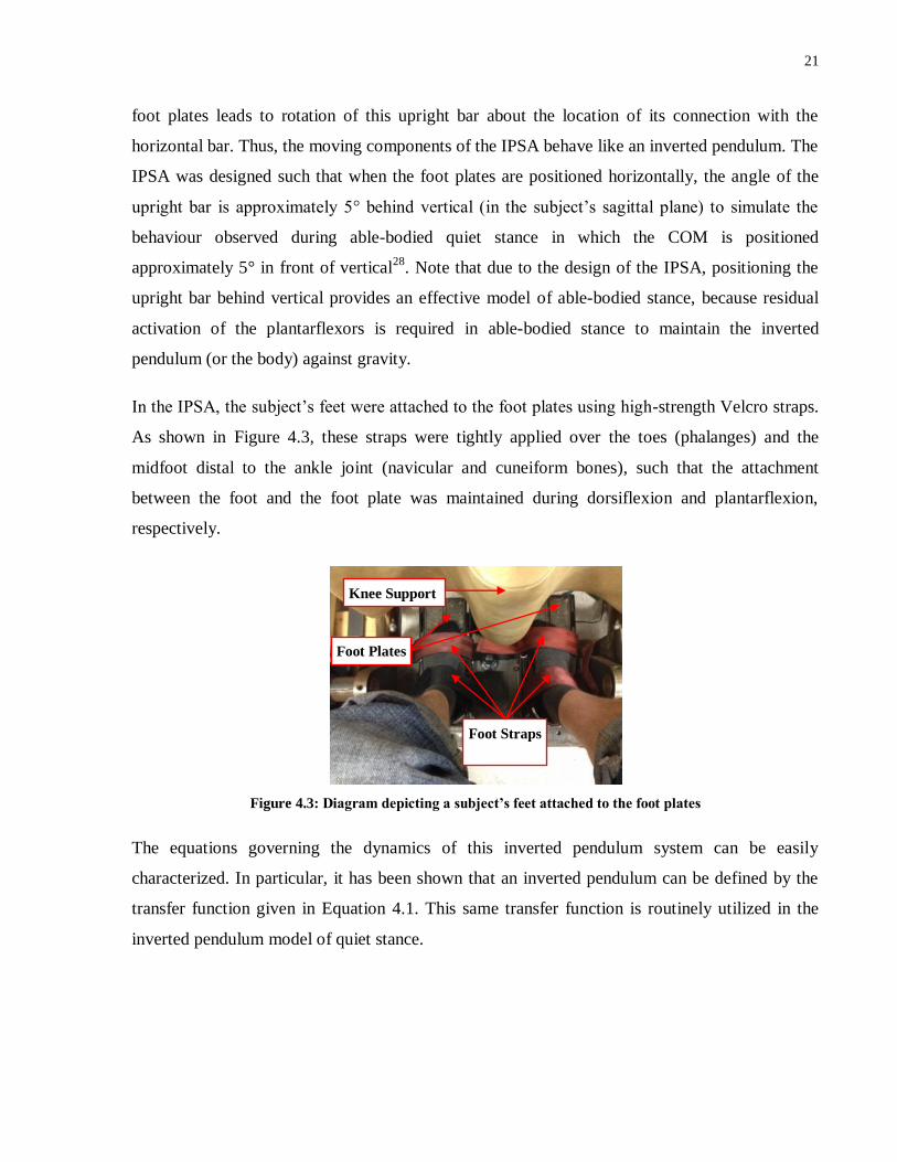
In the IPSA, the subject’s feet were attached to the foot plates using high-strength Velcro straps.
As shown in Figure 4.3, these straps were tightly applied over the toes (phalanges) and the
midfoot distal to the ankle joint (navicular and cuneiform bones), such that the attachment
between the foot and the foot plate was maintained during dorsiflexion and plantarflexion,
respectively.
Figure 4.3: Diagram depicting a subject’s feet attached to the foot plates
The equations governing the dynamics of this inverted pendulum system can be easily
characterized. In particular, it has been shown that an inverted pendulum can be defined by the
transfer function given in Equation 4.1. This same transfer function is routinely utilized in the
inverted pendulum model of quiet stance.
Foot Straps
Knee Support
Foot Plates

22
Equation 4.1: Transfer function defining the inverted pendulum
P(s) = transfer function of the plant (the inverted pendulum);
θ s = angle of the inverted pendulum;
(s) = torque acting on the inverted pendulum;
I = moment of inertia of the inverted pendulum;
m = mass of the inverted pendulum;
g = acceleration due to gravity; and
h = centre of mass height of the inverted pendulum
The total mass of the rotating parts has been calculated to be approximately 47.3 kg, with COM
height equal to 0.104 m and moment of inertia of 5.69 kg m2. These calculations were performed
by separating the IPSA into geometrically simple constituent parts and measuring the
dimensions, mass and COM height of each of these parts separately. Calculations could then be
performed to establish overall mass, COM height and moment of inertia.
The mass of the upright bar alone is 17.23 kg, with COM height equal to 0.34 m, and moment of
inertia of 5.52 kg m2. Extra weights were added to the inverted pendulum to increase the total
mass, COM height, and moment of inertia of the device, thus increasing the challenge of
controlling the device, and producing more physiologically relevant parameters. The calculated
parameters were used for defining the plant in the simulations discussed in Section 4.4.
The IPSA also contains a number of static components, including a base plate, locking
mechanism, safety stoppers and a standing frame. The locking mechanism allowed the inverted
pendulum to be locked in the neutral position with the foot plates horizontal, for use during
calibration and setup (see Section 4.3). The safety stoppers ensured that the inverted pendulum
did not rotate beyond approximately 14° behind vertical or 5° in front of vertical, so as to
guarantee that excessive strain was not applied to the ankles and that all potential movements
were within acceptable physiological ranges.
The standing frame (Ottobock, Germany) was positioned just in front of the foot plates as shown
in Figures 4.1 and 4.2, and comprised knee support and hip support components. Both of these
supports were cushioned in order to minimize discomfort. The knee support was positioned just
below and anterior to the knees over Tibia bones such that the knee joints were locked in an

23
extended position and were unable to bend. The knee support was positioned relative to the foot
plates such that the ankle joints were maintained at approximately 90° in the locked state. The
hip support was applied posterior to the subject once they were in a standing position. The bar
was positioned such that the hip support surfaces were located just below the buttocks bilaterally.
The hip supports included cushioned surfaces posterior to and lateral to the subject (see Figure
4.2), thus limiting A/P and medial/lateral (M/L) movement about the hips. The hip support was
locked in a position that was sufficiently tight to prohibit significant movement, but not so tight
as to induce excessive discomfort. The heights of both the knee and hip supports were variable,
as was the width of the hip support, so as to accommodate subjects of different sizes.
4.2.2 Other components
As shown in Figures 4.1 and 4.2, the setup also comprised a number of other components,
including:
1. A laser displacement sensor (LK2500, Keyence, Japan). This sensor, which was directed
towards the inverted pendulum in the A/P plane, recorded the displacement of the inverted
pendulum at a rate of 1,000 Hz. Following calibration and zeroing of the laser, simple
trigonometric calculations converted this displacement value into a measure of the inverted
pendulum’s angle which could be employed as input to the controller in real-time.
2. A torque transducer (TS11-200, Durham Instruments, Germany) was mounted to the
horizontal bar of the IPSA and it recorded the torque applied by the ankle muscles through
the footplates in real-time.
3. A programmable, 4-channel functional electrical stimulator (Compex Motion, Compex SA,
Switzerland) provided stimulation bilaterally to the plantarflexor and dorsiflexor muscles
through surface electrodes. For the purposes of these experiments, the stimulus waveform
was rectangular, charge balanced, biphasic and asymmetric. The frequency of stimulation
was fixed at 20 Hz, the pulse duration was fixed at 300 µs and the amplitude of stimulation
(in mA) was modulated depending on the controller output. These parameters were selected
based on experiments performed in our laboratory94
, as well as other studies95,96
which have
examined the effects of varying FES parameters on torque generation and rate of fatigue.
These parameters also allow for a sufficiently gradual rate of change of torque generation at
the minimum FES step size of 1 mA. In Experiments 1 and 2, the Compex Motion settings

24
resulted in a delay in changes in FES amplitude being applied of approximately 50 ms,
whilst in Experiment 3 this delay was decreased to approximately 10 ms.
4. A laptop running LabVIEW 2011 (National Instruments, USA).
5. A data acquisition device (NI USB-6211, National Instruments, USA), which facilitated
communication between the various devices.
6. A perturbation bar (Figure 4.4). The centre of this perturbation bar was attached to the
upright bar of the IPSA at a height of 0.93 cm during experiments in which anterior and
posterior external perturbations were applied (see Section 4.5.3.2). The bar, which weighed
2.00 kg, was fixed in the same plane as the inverted pendulum. Electromagnets were
attached to the perturbation bar at distances of 0.52 m anterior and posterior to the point of
attachment with the upright bar. During perturbation trials, each electromagnet supported a
weight of 2.33kg which could be released by switching off the electromagnets. The release
of each weight then induced anterior or posterior perturbations to the inverted pendulum.
Based on the assumption that the inverted pendulum was at the 5° reference angle when each
weight was dropped, the torque induced at the pivot point of the inverted pendulum could be
calculated using Equation 4.2. Thus, the anterior torque induced by dropping the posterior
weight was found to be 13.6 N.m, whilst the posterior torque induced by dropping the
anterior weight was 9.96 N.m. These parameters were selected in order to model
perturbations that can occur during the performance of activities of daily living while
standing. Specifically, they were designed to approximately match the torque induced about
the ankle joints when a typical person97
raises and lowers an arm rapidly through 90°.
Obviously the fact that the perturbations were instantaneous in our protocol added an
additional challenge.
Equation 4.2: Calculation of torque induced by dropping perturbation weights
= perturbing torque;
m = mass of the weight (2.33 kg);
g = acceleration due to gravity;
r = distance of the weight to the pivot point of the inverted pendulum;
θ = the angle of the weight position from vertical

25
Figure 4.4: The perturbation bar was used to apply external perturbations to the inverted pendulum by
removing power supplied to electromagnets and causing 2.33 kg weights to drop.
4.3 PID plus Gravity Control Strategies
4.3.1 Overview
Two distinct PID plus gravity control strategies were investigated, and the outcomes of
experiments and simulations using each control strategy were examined.
4.3.2 PID plus Gravity Controllers Outputting Required Torque
(Controller A)
The block diagram depicting Controller A, the initial control strategy examined, is shown in
Figure 4.5. In this system, an error signal was obtained by comparing the angle of the inverted
pendulum in real-time to a reference angle of 5°. This error signal (in radians) was then inputted
into separate PID controllers for the plantarflexors and dorsiflexors. Note that the sign of the
error signal was switched for one muscle group in order to account for the muscles producing
torque in opposite directions.
Inverted Pendulum
Added Weight
Perturbation Bar
Power Supply Electromagnets
Holding 2.33 kg
Weights

26
Figure 4.5: Block diagram depicting the first PID plus gravity control strategy (Controller A)
The composition of each PID controller block from Figure 4.5 is depicted in Figure 4.6 and
summarized in Equation 4.3. Each PID controller comprised 3 components which operated in
parallel:
i. A proportional component, which varied in proportion to changes in the angle of the
inverted pendulum relative to the reference angle. The relative contribution of this
component was dictated by the value of the gain KP.
ii. A derivative component, which varied in proportion to changes in the angular velocity of the
inverted pendulum, and whose relative contribution was dictated by the value of the gain KD.
This component also included a derivative filter term (N) which ensured that the derivative
term did not result in unwanted amplification of high frequency noise. Note that in practice,
given the high level of accuracy of the laser displacement sensor employed in experiments,
high frequency noise was not a major concern in this protocol. However, the derivative filter
was included for completeness and to avoid practical difficulties when attempting to run
simulations with an inherently unstable derivative component. In all experiments, the
derivative filter term N was fixed at 150 for both muscle groups, resulting in minimal impact
on the operation of the control system.
It is also noteworthy that the PID controllers were formatted such that the derivative gain KD
was expressed as a proportion of the proportional gain KP. This configuration, which is often
utilized in the ‘standard’ or ‘ideal’ form of a PID controller98
, was employed to improve the
ease of tuning the gains. Since the ratio of the derivative gain to the proportional gain is
FES
Current
)θsin( out hgm
Requested
Torque
θref+-
Requested
Torque
YES
NOFES
Current
θout
Gravity Compensator
+-
-1 ++PID
Controller
PID
Controller
> 0
Muscle
Recruitment Curve
Muscle
Recruitment Curve
Plantarflexors
DorsiflexorsInverted
Pendulum
Plantarflexors
Dorsiflexors
Torq
ue
Current
Torq
ue
Current

27
often a more relevant indicator of the relative contribution of the derivative component, it
was useful to have this ratio encompassed in a single gain value.
iii. An integral component which varied in proportion to the sum of all previous error signals,
and whose relative contribution was dictated by the value of the gain KI. If the sign of the
error signal remained the same for a prolonged period, the contribution of this component
would grow in order to bring the inverted pendulum angle back to the reference angle.
Therefore, this component was employed in order to minimize steady state error.
Figure 4.6: PID controller configuration employed.
Equation 4.3: Transfer function defining the PID controllers
C(s) = transfer function of the PID controller;
KP = proportional gain;
KI = integral gain;
KD = derivative gain; and
N = derivative filter gain.
The structure of the PID controllers for the plantarflexors and dorsiflexors was identical, but the
values of the gains could differ. In this first configuration, the outputs of the plantarflexor and
dorsiflexor PID controllers gave measures of requested torque in the direction of increasing
plantarflexor and dorsiflexor activation, respectively.
In order to account for the varying effects of gravity with inverted pendulum angle, a gravity
compensation term was incorporated at the outputs of the PID controllers. The gravity
compensation term, defined in Equation 4.4, gave a real-time measure of the torque due to
KP
KD +- N
s
1
++
KIs
1
++
Derivative
Gain
Integral Gain
Proportional
Gain
Derivative
Filter Term
Input Output

28
gravity acting on the inverted pendulum. Since the reference angle was positioned posteriorly,
the plantarflexors needed to produce torque so as to compensate for the effect of gravity, whilst
gravity operated in the same direction as the dorsiflexors. Thus, in order to counteract the effect
of gravity, this gravity compensation term was added to the output of the plantarflexor PID
controller, and subtracted from the output of the dorsiflexor PID controller.
Equation 4.4: Gravity compensation term
s
g = torque due to gravity (Nm)
θ = angle of the inverted pendulum (relative to vertical);
m = mass of the inverted pendulum;
g = acceleration due to gravity; and
h = centre of mass height of the inverted pendulum
In order to minimize fatigue caused by unnecessary muscle stimulation, a condition was
incorporated to ensure that only one muscle group was active at any given time. Since the
plantarflexors are larger and more important than the dorsiflexors in the control of standing
stability28
, this condition was based on the real-time required plantarflexor torque calculated. If
this torque was positive, indicating that the plantarflexors should be activated, the dorsiflexors
would not be stimulated. Thus, for the dorsiflexors to be stimulated, the plantarflexor requested
torque had to be zero or negative, and the dorsiflexor requested torque had to be greater than
zero.
In order to determine the amplitude of FES to apply in real-time, the requested torques had to be
converted into corresponding FES levels. This was achieved using muscle recruitment curves,
which were obtained for each subject with the inverted pendulum locked in the neutral position
(i.e., positioned at a 5° angle posterior to vertical) and the subject in a standing position in the
IPSA. The paradigm involved running LabVIEW code that applied varying FES intensities and
recorded the resultant isometric torques generated through the footplates in real time using the
torque transducer mentioned in Section 4.2.2. Isometric torque recruitment curves were
appropriate for this experiment since the ankle angle did not typically fluctuate by more than +/-
5° during the experiments from the nominal angle of 5°, indicating that length and velocity
components of the muscle contraction dynamic did not play any significant role.

29
Initially, a baseline torque, produced by the subject’s passive standing posture, was recorded.
The FES was then applied to the plantarflexors starting at 15 mA up to 60 mA in divisions of 5
mA, followed by the dorsiflexors from 15 mA up to 45 mA in divisions of 5 mA. Note that the
lower maximum intensity applied to the dorsiflexors was a consequence of these muscles being
smaller and therefore saturating at lower current amplitudes. As a result, it was observed that
stimulation above 45 mA typically resulted in minimal increases in generated torque, but did
cause increased discomfort and fatigue. The stimulation followed a 5-second on, 5-second off
paradigm for both muscles so as to avoid excessive fatigue, whilst still allowing the generated
torque to typically reach a steady state.
Figures 4.7 (a) and (b) depict typical muscle recruitment curves for an able-bodied individual’s
plantarflexors and dorsiflexors, respectively. From these curves, the set of FES amplitudes
applied can be mapped to the corresponding torques created. At each FES amplitude, the mean
torque achieved was defined as the average torque over the final 3 seconds of the 5-second
stimulation period. This is because, as seen in Figure 4.6, there was a ramp-up period prior to
near-maximal torque being reached. The baseline torque was then subtracted from each
measured torque value in order to establish the torque generated at each current level applied.
Based on these muscle recruitment curves, look-up tables were created for each subject on each
experimentation day. Thus, the required torque levels outputted by the PID plus gravity
controllers were converted to required FES current levels for each muscle. Within each 5 mA
step, linear interpolation was performed in order to establish the requisite current to the nearest
mA. However, based on observation, current levels below 20 mA typically produced little to no
torque, and as such requisite current levels below 20 mA resulted in stimulation to that muscle
being switched off. Similarly, at requested torques corresponding to current amplitudes in excess
of the maximum allowable intensity (60 mA for plantarflexors, 45 mA for dorsiflexors), these
maximum currents were selected.

30
Figure 4.7: Muscle recruitment curves for (a) plantarflexors and (b) dorsiflexors, for use with Controller A.
The blue lines represent the continuous torque recordings during intermittent 5-second periods of increasing
stimulation current amplitude. The maroon markers represent the established torque values at each FES
amplitude, and the maroon lines represent the linear interpolations that were utilized in between FES
amplitude levels.
Ultimately, the current levels were applied to at most one muscle group at any given time,
inducing torque and causing the inverted pendulum to move. This movement was recorded by
the laser displacement sensor and the inverted pendulum angle was fed back to create a new error
signal input. Simulations and experiments in 3 able-bodied subjects were performed with this
control strategy.
In this experiment, the sampling frequency of the controller software was set to 100 Hz. Thus,
10 15 20 25 30 35 40 45 50 55 60
0
50
100
150
200
0 20 40 60 80 100
Current Amplitude (mA)
Torq
ue
(N
m)
Time (seconds)
(a) Plantarflexor Recruitment Curve
10 15 20 25 30 35 40 45
-10
-5
0
5
10
15
20
25
0 20 40 60 80
Current Amplitude (mA)
Torq
ue
(N
m)
Time (seconds)
(b) Dorsiflexor Recruitment Curve
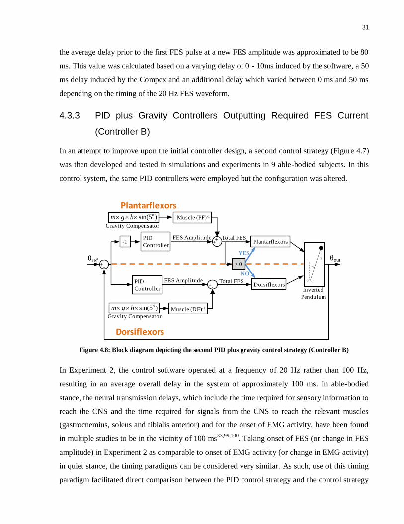
31
the average delay prior to the first FES pulse at a new FES amplitude was approximated to be 80
ms. This value was calculated based on a varying delay of 0 - 10ms induced by the software, a 50
ms delay induced by the Compex and an additional delay which varied between 0 ms and 50 ms
depending on the timing of the 20 Hz FES waveform.
4.3.3 PID plus Gravity Controllers Outputting Required FES Current
(Controller B)
In an attempt to improve upon the initial controller design, a second control strategy (Figure 4.7)
was then developed and tested in simulations and experiments in 9 able-bodied subjects. In this
control system, the same PID controllers were employed but the configuration was altered.
Figure 4.8: Block diagram depicting the second PID plus gravity control strategy (Controller B)
In Experiment 2, the control software operated at a frequency of 20 Hz rather than 100 Hz,
resulting in an average overall delay in the system of approximately 100 ms. In able-bodied
stance, the neural transmission delays, which include the time required for sensory information to
reach the CNS and the time required for signals from the CNS to reach the relevant muscles
(gastrocnemius, soleus and tibialis anterior) and for the onset of EMG activity, have been found
in multiple studies to be in the vicinity of 100 ms33,99,100
. Taking onset of FES (or change in FES
amplitude) in Experiment 2 as comparable to onset of EMG activity (or change in EMG activity)
in quiet stance, the timing paradigms can be considered very similar. As such, use of this timing
paradigm facilitated direct comparison between the PID control strategy and the control strategy
)5sin( o hgm
FES Amplitude
θref+-
FES Amplitude
YES
NO
θout
Gravity Compensator
++PID
Controller
PID
Controller
> 0
Plantarflexors
DorsiflexorsInverted
Pendulum
Plantarflexors
Dorsiflexors
Muscle (PF)-1
)5sin( o hgm
Gravity Compensator
Muscle (DF)-1
+-
Total FES
Total FES
-1
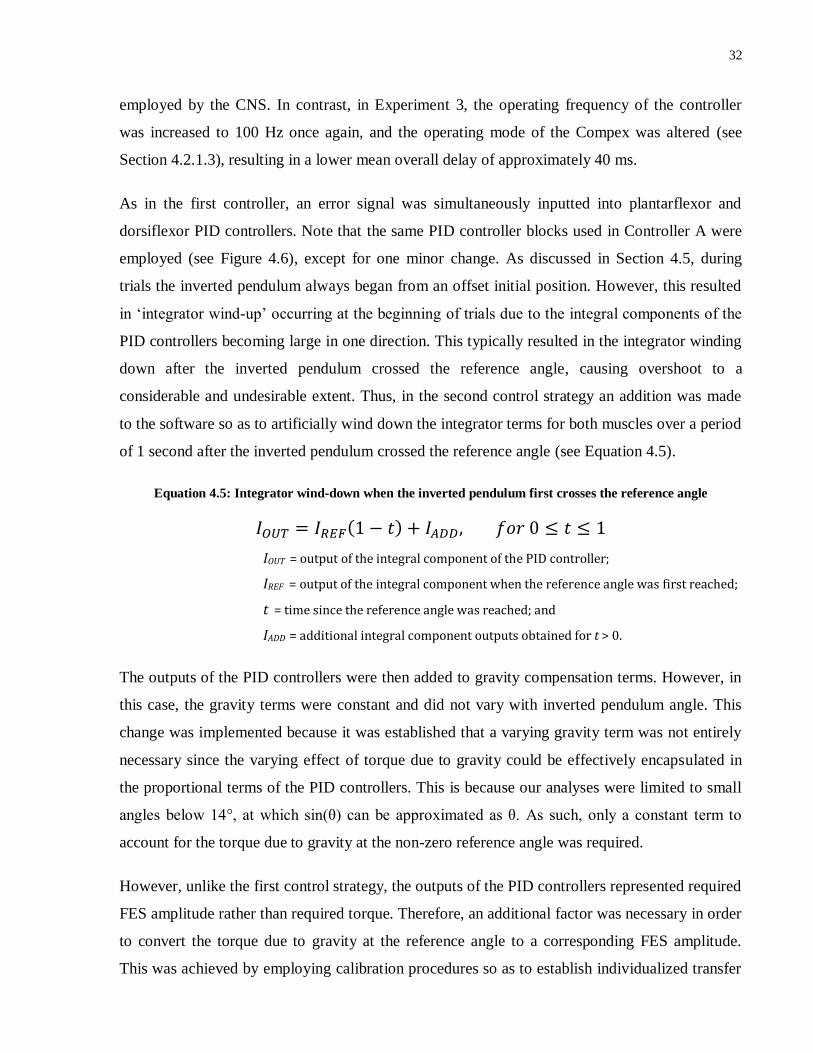
32
employed by the CNS. In contrast, in Experiment 3, the operating frequency of the controller
was increased to 100 Hz once again, and the operating mode of the Compex was altered (see
Section 4.2.1.3), resulting in a lower mean overall delay of approximately 40 ms.
As in the first controller, an error signal was simultaneously inputted into plantarflexor and
dorsiflexor PID controllers. Note that the same PID controller blocks used in Controller A were
employed (see Figure 4.6), except for one minor change. As discussed in Section 4.5, during
trials the inverted pendulum always began from an offset initial position. However, this resulted
in ‘integrator wind-up’ occurring at the beginning of trials due to the integral components of the
PID controllers becoming large in one direction. This typically resulted in the integrator winding
down after the inverted pendulum crossed the reference angle, causing overshoot to a
considerable and undesirable extent. Thus, in the second control strategy an addition was made
to the software so as to artificially wind down the integrator terms for both muscles over a period
of 1 second after the inverted pendulum crossed the reference angle (see Equation 4.5).
Equation 4.5: Integrator wind-down when the inverted pendulum first crosses the reference angle
IOUT = output of the integral component of the PID controller;
IREF = output of the integral component when the reference angle was first reached;
t = time since the reference angle was reached; and
IADD = additional integral component outputs obtained for t > 0.
The outputs of the PID controllers were then added to gravity compensation terms. However, in
this case, the gravity terms were constant and did not vary with inverted pendulum angle. This
change was implemented because it was established that a varying gravity term was not entirely
necessary since the varying effect of torque due to gravity could be effectively encapsulated in
the proportional terms of the PID controllers. This is because our analyses were limited to small
angles below 14°, at which sin(θ) can be approximated as θ. As such, only a constant term to
account for the torque due to gravity at the non-zero reference angle was required.
However, unlike the first control strategy, the outputs of the PID controllers represented required
FES amplitude rather than required torque. Therefore, an additional factor was necessary in order
to convert the torque due to gravity at the reference angle to a corresponding FES amplitude.
This was achieved by employing calibration procedures so as to establish individualized transfer

33
functions to represent the muscle dynamics of each muscle in each subject.
This calibration was performed with the subject in a standing position, and the IPSA locked in
the neutral position. Sinusoidal varying FES amplitudes between 20 mA and 60 mA were then
applied to the plantarflexors, and the resulting isometric torque patterns were recorded. The
sinusoidal variations were applied at frequencies of 0.07 Hz, 0.15 Hz, 0.3 Hz, 0.75 Hz, and 1.2
Hz. Higher frequencies were not tested due to limitations on the Compex stimulator’s operating
frequency. The durations of these trials varied depending on the frequency, but lasted at least 10
seconds and at least long enough to record 2 complete periods. The same trials were then
completed for the dorsiflexors.
Figures 4.9 and 4.10 depict typical results of these calibration trials in a single subject for the
plantarflexors and dorsiflexors, respectively. In these figures, the green dashed curves
correspond to the current amplitudes, whilst the blue waveforms represent the torque outputs.
The red curves represent sinusoidal curves of best fit to the torque output curves, at the same
frequencies as the sinusoidally varying current amplitudes. In order to avoid transient effects, the
beginning of each trial was disregarded when fitting the torque output curves to sinusoids. In the
calibrations performed in able-bodied subjects in Experiment 2 (see Section 4.5.3), only the first
second of each trial was disregarded, but in subsequent simulations and Experiment 3 (and in the
figures shown) the first 5 seconds of each trial was disregarded. In addition, constant delays of
120 ms initially for Experiment 2 and 40 ms for Experiment 3 were separated out when applying
the sinusoidal fitting so that the torque generation delays of the muscles could be examined
independent of the hardware delays. The values of these delays were selected based on the
approximate delays prior to the onset of any torque generation in response to step FES inputs
(like those used in the calibration procedure for Controller A - see Section 4.3.2). These values
corresponded approximately with the estimated hardware delays in each experiment.
The amplitude and phase difference between the input signal and the fitted output signal were
calculated at each frequency. From these data, first-order models of the muscle dynamics of the
form shown in Equation 4.6 were created using the Matlab (Mathworks, USA) function invfreqs,
which identifies transfer functions of predefined order based on frequency response data. Bode
plots were then created for the amplitude and phase difference data and for the suggested first
order transfer functions. Figure 4.11 depicts scatterplots (black crosses) of the bode plots

34
corresponding to the input/output plots in Figures 4.9 and 4.10. The bode plots of the transfer
functions calculated for these data for each muscle are depicted by the solid lines on the same set
of axes. From these graphs, it is evident that there is generally good agreement between the
experimental and predicted data. Root mean square error (RMSE) values and correlation
coefficients between the observed and predicted data were also calculated so as to quantify the
degree of fit of the first-order model. A first-order model was selected based on observations that
the quality of fit was typically comparable or better than that observed with higher order models.
Further analysis of the appropriateness of this model is presented in the Results.
Equation 4.6: First-order model of muscle dynamics
M(s) = transfer function of the muscle;
K = factor dictating the gain of the muscle;
α = factor dictating the transient muscle behaviour;
These first-order models were then utilized in simulations (see Sections 4.4.2 and 4.4.3) as well
as for calculating the controller’s gravity compensation components. The inverses of the muscle
transfer functions were approximated as 1/K (see Equation 4.6) for each muscle. Then, with the
addition of the gravity terms, the outputs of the PID plus gravity controllers (as FES amplitudes)
could be applied directly to either the plantarflexors or dorsiflexors. As in Controller A, the
switching condition was controlled based on the output of the plantarflexor’s PID plus gravity
controller.
Note that this control strategy (Controller B) offered the benefit over the first control strategy
(Controller A) of providing information on the dynamics of the muscles of each subject,
including torque generation delays. However, unlike the first control strategy, this technique did
not account for the complex relationship between FES amplitude and torque saturation level (i.e.,
the steady state torques achieved following the torque generation delay period). Rather, a linear
relationship was assumed between torque saturation level and FES current levels between 20 mA
and 60 mA for plantarflexors, and between 20 mA and 45 mA for dorsiflexors. An in-depth
comparison of the two control strategies is presented in the Discussion.

35
Figure 4.9: Calibration curves used for defining the muscle dynamics of the plantarflexors in Controller B. In
each plot, the green dashed curves represent inputted sinusoidally-varying current amplitudes, whilst the
blue curves represent the subsequent torque outputs. The red curves depict sinusoidal waveforms of best fit
to the torque output curves (after subtracting the initial 5 seconds). The frequency of the green and red
sinusoidal waveforms is listed for each plot.

36
Figure 4.10: Calibration curves used for defining the muscle dynamics of the dorsiflexors in Controller B. In
each plot, the green dashed curves represent inputted sinusoidally-varying current amplitudes, whilst the
blue curves represent the subsequent torque outputs. The red curves depict sinusoidal waveforms of best fit
to the torque output curves (after subtracting the initial 5 seconds). The frequency of the green and red
sinusoidal waveforms is listed for each plot.

37
Figure 4.11: Bode plots of phase and amplitude response data obtained experimentally (black crosses), and
corresponding bode plots from the first-order muscle dynamics transfer function calculated (solid blue lines).
4.4 Simulations
Simulations were performed using Simulink (Mathworks, USA) for a number of reasons:
i. To establish initial controller parameters for use in experiments (Controller B);
ii. To investigate the mechanisms behind experimental results obtained (both controllers);
iii. To gauge the limitations of the theoretical models of system behaviour (both controllers);
and
iv. To investigate the stability of the controllers at the parameters employed (both
controllers).
4.4.1 Simulations using Controller A
Simulations were performed with Controller A after completing experiments in 3 able-bodied
subjects. The design of the Simulink model is depicted in Figure 4.12. In this model, 40-second
simulations were performed during which an offset initial inverted pendulum position, step
responses in each direction, and external perturbations in each direction, were incorporated. At
the input to the simulation, the initial offset position was modelled using a negative step function,
whilst the step response was modelled using a pulse of 8-second duration that shifted the
reference angle from 5° to 9°. External anterior and posterior perturbations were modelled as
short duration torques added to the plant (i.e., the inverted pendulum). In Figure 4.12, the two

38
PID controllers and the gravity compensation component, discussed in Section 4.3.2, are
highlighted. However, additional components were also added to the controller depicted in
Figure 4.5 in order to model the experimental behaviour of the system.
At the outputs of the PID plus gravity controllers, saturation blocks were included in order to
account for the maximum producible torque of each individual and for the fact that FES cannot
induce negative torque (i.e., torque in the direction opposite the direction of normal torque
production in that muscle). Thus, the minimum limits of the saturation blocks were set to 0,
whilst the maximum limits were defined based on the subject-specific torques produced at the
maximum current amplitudes tested during calibration (60 mA for plantarflexors, 45 mA for
dorsiflexors).
After the saturation blocks, a constant time delay was also incorporated in order to account for
both the delays in the setup (e.g., the 10 Hz refresh rate of the Compex) and the torque
generation delays of the muscles. A constant delay of 120 ms was selected for each muscle in
each subject based on analysis of typical calibration curves obtained, and by attempting to obtain
optimal matching characteristics between the outputs of simulations and the results of the
experimental trials. Note that muscle recruitment nonlinearities were not modelled with
Controller A, thus allowing for testing of the ability of constant delays to model system
behaviour. In later simulations, models of nonlinear muscle dynamics were incorporated (see
Section 4.4.2).
The total torque was then applied to a state space representation of the inverted pendulum with
the same amount of weight added as in experiments. This state space representation was obtained
by applying the tf2ss Matlab function on the transfer function defined in Equation 4.1. A state
space representation was employed so as to allow for analysis from a non-zero initial position in
Simulink. This also required the addition of an ‘Initialize Subsystem’ in order to model the initial
situation in which the inverted pendulum was resting on supports at an angle of approximately
14°. This subsystem is depicted in Appendix A.

39
Figure 4.12: Simulink model used for simulating system behaviour with Controller A.
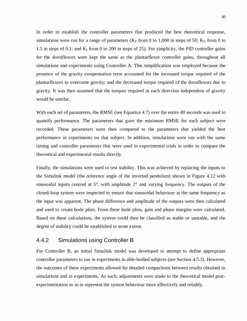
40
In order to establish the controller parameters that produced the best theoretical response,
simulations were run for a range of parameters (KP from 0 to 1,000 in steps of 50; KD from 0 to
1.5 in steps of 0.1; and KI from 0 to 200 in steps of 25). For simplicity, the PID controller gains
for the dorsiflexors were kept the same as the plantarflexor controller gains, throughout all
simulations and experiments using Controller A. This simplification was employed because the
presence of the gravity compensation term accounted for the increased torque required of the
plantarflexors to overcome gravity; and the decreased torque required of the dorsiflexors due to
gravity. It was then assumed that the torques required in each direction independent of gravity
would be similar.
With each set of parameters, the RMSE (see Equation 4.7) over the entire 40 seconds was used to
quantify performance. The parameters that gave the minimum RMSE for each subject were
recorded. These parameters were then compared to the parameters that yielded the best
performance in experiments on that subject. In addition, simulations were run with the same
timing and controller parameters that were used in experimental trials in order to compare the
theoretical and experimental results directly.
Finally, the simulations were used to test stability. This was achieved by replacing the inputs to
the Simulink model (the reference angle of the inverted pendulum) shown in Figure 4.12 with
sinusoidal inputs centred at 5°, with amplitude 2° and varying frequency. The outputs of the
closed-loop system were inspected to ensure that sinusoidal behaviour at the same frequency as
the input was apparent. The phase difference and amplitude of the outputs were then calculated
and used to create bode plots. From these bode plots, gain and phase margins were calculated.
Based on these calculations, the system could then be classified as stable or unstable, and the
degree of stability could be established to some extent.
4.4.2 Simulations using Controller B
For Controller B, an initial Simulink model was developed to attempt to define appropriate
controller parameters to use in experiments in able-bodied subjects (see Section 4.5.3). However,
the outcomes of these experiments allowed for detailed comparisons between results obtained in
simulations and in experiments. As such, adjustments were made to the theoretical model post-
experimentation so as to represent the system behaviour more effectively and reliably.

41
4.4.2.1 Initial Simulations
The Simulink model employed for selecting initial parameters to use for each subject in
experiments is depicted in Figure 4.13. This model utilized the same 40-second simulation
period, during which offset initial position, step responses and anterior and posterior
perturbations were applied, using the same method discussed in the previous section. This model
also employed the same PID control structure, although integral reset subsystems were also
added to wind down the integral terms once the model compensated for the offset initial position.
This integral reset subsystem is presented in Appendix A. The same state space model of the
inverted pendulum was also implemented.
As in the Controller B model depicted in Figure 4.7, gravity terms were included based on each
subject’s first-order muscle dynamics models obtained during calibrations. Note that the 1/K1
and 1/K2 blocks correspond to ratios of the gains of the muscle dynamics blocks for each muscle
(shown in light blue). These blocks were included in the model such that the PID plus gravity
controller outputs, which are measures of required current amplitudes, could be converted to
required torque levels to be inputted into the inverted pendulum model. Also note that the 120 ms
constant delay that was removed from calculations of the muscle dynamics has also been added
to the model. Saturation blocks were also present, limiting the controller outputs to 0 to 40 (or
maximum current level requested by the subject in experiments) for the plantarflexors and 0 to
25 (or maximum current level requested) for the dorsiflexors. With the addition of the 20 mA
minimum level below which the current amplitude drops to 0 mA, these values correspond to the
minimum and maximum current levels used (i.e. 20 mA to 60 mA for plantarflexors; and 20 mA
to 45 mA for dorsiflexors). In this model, the criterion for switching between muscles was tested
after the constant delay but before the muscle dynamics blocks. However, this criterion was
implemented after the muscle dynamics blocks.
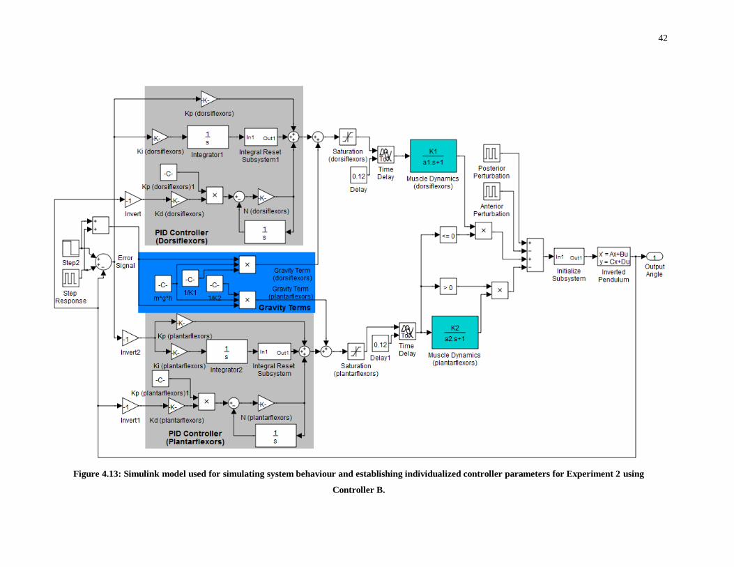
42
Figure 4.13: Simulink model used for simulating system behaviour and establishing individualized controller parameters for Experiment 2 using
Controller B.

43
In order to select initial parameters for use in experiments (see Section 4.5.3), simulations with
each subject’s individual muscle models (and saturation limits) were performed over a range of
PID controller parameters (KP from 80 to 300 in steps of 10; KD from 0.2 to 1.1 in steps of 0.05;
and KI from 0 to 100 in steps of 25). The dorsiflexor derivative and integral gains were set equal
to the plantarflexor gains, whilst the dorsiflexor proportional gain was fixed at 500. These
dorsiflexor gain parameters were chosen based on the results of preliminary experiments and
simulations in 2 subjects. As in the previous section, the parameters that gave the lowest total
RMSE (see Equation 4.7) were recorded. If any of the parameters that minimized RMSE were
within 10% of the limits examined, then these limits were expanded and the simulations were
repeated. From the parameters obtained, each gain (KP, KD and KI) was decreased by 25%, and
these final gain values were then used as the initial parameters employed in experiments. This
25% reduction was performed based on the assumption that the parameters that minimized
RMSE would not necessarily maximise stability; and that small, proportional decreases in gain
values would likely improve stability (whilst decreasing speed of response). These assumptions
were verified in preliminary experiments.
4.4.2.2 Improvements to Simulations Post-Experimentation
Following the completion of experiments in able-bodied subjects, the Simulink model and
calibration procedure were adjusted so as to better match and therefore explain experimental
results, and to provide a more realistic, physiologically relevant model of the system’s behaviour.
The revised Simulink model is presented in Figure 4.14. A number of changes were
implemented:
i. The structure of the criterion for switching between muscles was reconfigured. First, the
switching criterion was positioned prior to the constant time delay terms so as to better
represent the experimental situation in which the programmatic switching between muscles
could be performed with minimal delay and independent of the delays caused by the
Compex stimulator. Second, the switching criterion was enacted prior to the muscle
dynamics blocks. This avoided the physiologically unrealistic situation in which torque
produced by each muscle would rapidly drop to zero at the onset of a switch. Rather the rate
of decrease in torque after the stimulation was removed was dictated by the muscle
dynamics transfer functions. Although these transfer functions typically underestimated the

44
rate of torque decrease, this still represented a more physiologically accurate representation.
ii. The effect of the intrinsic mechanical properties of the lower limbs was incorporated into the
design through the inclusion of a ‘passive contribution’ component, highlighted in green. In
models of quiet standing, this passive contribution has been routinely incorporated, in
combination with an active component30,32,33,36
. As in these previous studies, a rotational
stiffness gain was included which varied in response to changes in the error signal, as well as
a rotational viscosity gain which varied in relation to the rotational velocity of the inverted
pendulum. The values of these gains were selected based on the literature30,32,33,36,101,102
, and
by comparing the simulation outputs to experimental results (see the Results section).
iii. A ‘voluntary contribution’ component was also incorporated. Whilst the inverted pendulum
helps to disrupt voluntary control, it is unreasonable to suggest that voluntary control would
be absent. In particular, a voluntary damping factor was utilized in order to account for the
contribution of voluntary control in opposition to rotational velocity. The addition of this
component makes some intuitive sense given that the CNS is likely to automatically activate
muscles to some extent in response to rapid movements of the inverted pendulum in order to
avoid destabilization. Automatic postural adjustments, characterized by muscle activation in
response to external perturbations so as to counteract the perturbation and avoid instability,
are well documented99,100
. Thus, by considering fluctuations in FES intensity as external
perturbations, it is logical to consider that automatic postural adjustments, regulated by the
CNS, will act to oppose these perturbations. Whilst the exact mechanisms and magnitudes of
these postural adjustments may not be equivalent to those observed during actual stance,
some postural adjustments are considered inevitable. Note that unlike the passive control
component, a delay was incorporated to account for the neural-mechanical delay involved in
active voluntary control. The value of this delay was set based on previous studies that
recorded onset of EMG activity in the tibialis anterior, gastrocnemius and soleus muscles
during perturbed stance99,100
. A small additional delay was also incorporated to account for
the torque generation delay, giving a total delay of 120 ms. The voluntary damping gain was
varied to obtain best agreement with experimental outcomes (see Results).
iv. The structure of the constant time delay was altered. Instead of a constant delay of 120 ms, a
time delay of 50 ms was incorporated on either side of 50 ms Hold blocks. These Hold

45
blocks discretized the signal every 50 ms. The first Hold blocks encountered by each muscle
account for the discretizing of the signal based on the 20 Hz operating frequency of the
controller software. Then, the 50 ms constant delay corresponds to the delay induced by the
Compex. Finally, an additional 50 ms Hold block was incorporated to account for a potential
additional delay of up to 50 ms depending on the timing of the next Compex pulse. The
inclusion of these discretizing signals was considered a more accurate representation of the
system behaviour, given that the actual delay prior to FES amplitude changes would not be
constant but would depend on the timing of the software and the Compex. In Experiment 3,
the first Hold block was altered so as to discretize the signal every 10 ms in accordance with
the 100 Hz operating frequency of the controller. Similarly, the 50 ms constant time delay
was changed to 10 ms to account for the shorter delay induced by the Compex.
These adjustments induced average time delays of 100 ms for Experiment 2 and 40 ms for
Experiment 3, which were also factored into the calculation of each muscle’s transfer
function.

46
Figure 4.14: Simulink model for Controller B including adjustments made post-experimentation

47
4.5 Experimentation in Able-Bodied Subjects
Preliminary experiments were performed in 3 able-bodied subjects using Controller A (see
Section 4.3.2), and subsequent experiments were performed in 11 able-bodied subjects using
Controller B (see Section 4.3.3).
4.5.1 Initial setup
Prior to beginning experiments, each subject gave written informed consent to participate in the
experimental protocol, which was approved by the local ethics committee in accordance with the
Declaration of Helsinki. All subjects were able-bodied individuals with no known neurological
or musculoskeletal disorders. Basic anthropometric data (age, height and weight) was also
obtained.
Electrodes were then applied. For plantarflexion, 5 cm x 9 cm electrodes were applied bilaterally
along the midline of the posterior calf. The anode was placed approximately 2 - 3 cm below the
knee joint over the gastrocnemius and soleus muscle motor points so as to activate both
gastrocnemius heads as well as the soleus muscle. The cathode was placed just above the ankle
joint. For dorsiflexion, 5 cm 5 cm electrodes were applied bilaterally to the anterior calf. Note
that the smaller electrodes are a consequence of the dorsiflexing muscles (mainly tibialis
anterior) being much smaller than their plantarflexing counterparts. The anode was placed over
the motor point of the tibialis anterior, just lateral to the fibula, and the cathode was placed
approximately 8 – 10 cm below the anode. Thus, a total of 8 electrodes were applied. The
approximate positions of the electrodes are highlighted in Figure 4.15. During application, gel
was applied to increase skin conductivity.
Following the application of electrodes, the subject was positioned in a standing posture in the
IPSA, which was locked in the neutral position. The foot straps and knee and hip supports were
applied (see Section 4.2.1.3 for more details), and the electrodes were attached to the Compex
stimulator.
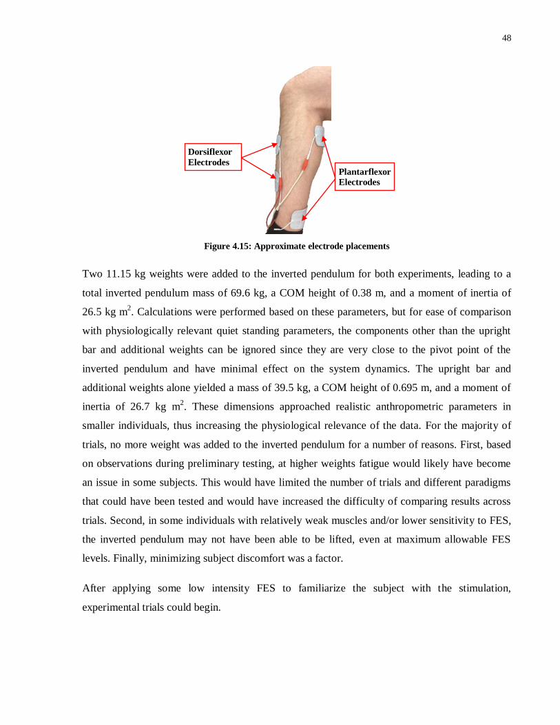
48
Figure 4.15: Approximate electrode placements
Two 11.15 kg weights were added to the inverted pendulum for both experiments, leading to a
total inverted pendulum mass of 69.6 kg, a COM height of 0.38 m, and a moment of inertia of
26.5 kg m2. Calculations were performed based on these parameters, but for ease of comparison
with physiologically relevant quiet standing parameters, the components other than the upright
bar and additional weights can be ignored since they are very close to the pivot point of the
inverted pendulum and have minimal effect on the system dynamics. The upright bar and
additional weights alone yielded a mass of 39.5 kg, a COM height of 0.695 m, and a moment of
inertia of 26.7 kg m2. These dimensions approached realistic anthropometric parameters in
smaller individuals, thus increasing the physiological relevance of the data. For the majority of
trials, no more weight was added to the inverted pendulum for a number of reasons. First, based
on observations during preliminary testing, at higher weights fatigue would likely have become
an issue in some subjects. This would have limited the number of trials and different paradigms
that could have been tested and would have increased the difficulty of comparing results across
trials. Second, in some individuals with relatively weak muscles and/or lower sensitivity to FES,
the inverted pendulum may not have been able to be lifted, even at maximum allowable FES
levels. Finally, minimizing subject discomfort was a factor.
After applying some low intensity FES to familiarize the subject with the stimulation,
experimental trials could begin.
Plantarflexor
Electrodes
Dorsiflexor
Electrodes
49
4.5.2 Experiment 1: Preliminary experiments in 3 subjects (Controller A)
4.5.2.1 Preparation
First, calibration was performed using the procedure outlined in Section 4.3.2, in order to obtain
muscle recruitment curves for each muscle. Following the calibration trials, the subject was
allowed to rest for at least 3 minutes in order to minimize the likelihood of fatigue. This
timeframe was selected because the majority of recovery has been reported to occur within the
first few minutes of rest103,104
. Breaks of similar duration were implemented throughout both
experimental protocols.
The IPSA was unlocked such that the inverted pendulum was free to rotate, and the laser
displacement sensor was zeroed using a digital level. The inverted pendulum was then brought to
rest on a support surface approximately 14° behind vertical. Controller parameters were then
designated in the LabVIEW program. In Subject 1, these parameters were initially selected based
on the results of previous studies performed by our lab and others29,30,54
. However, the
parameters were then tuned based on performance during preliminary trials. In Subjects 2 and 3,
the initial parameters were selected based on the parameters ultimately used in Subject 1, but
were also tuned based on performance as necessary.
4.5.2.2 Trials - FES Condition:
In the FES Condition, FES was applied to the plantarflexors and dorsiflexors based on the
outputs of the control structures outlined in Section 4.3. In this condition, the subject was
instructed to have eyes closed so as to minimize any voluntary control of balance. This resulted
in a disruption to visual sensory information on top of the disruption to vestibular inputs caused
by use of the IPSA. The subject was instructed to stand with arms crossed on his/her chest, and
to attempt to relax and suppress voluntary control of muscle contractions as much as possible.
Brief, 10-20 second trials were then initiated in order to test the performance of the controller
and to elucidate whether changes to controller gains were required. During each trial, the real-
time inverted pendulum angle, and plantarflexor and dorsiflexor current levels were recorded.
Since the inverted pendulum began at an angle of 14° behind vertical, activation of the
plantarflexors was initially required to bring the inverted pendulum to the reference angle of 5°.
Thus, the ability of the controller to overcome this offset initial position rapidly and to avoid
50
instability, excessive overshoot or prolonged oscillations could be examined.
Manual PID tuning procedures were implemented in order to fine-tune the parameters to yield
successful control of the inverted pendulum. These tuning procedures were based on previous
studies105,106
and preliminary research. During tuning, controller gains were only altered by 10%
or more on each occasion, so as to limit the number of iterations required to tune the controller.
Moreover, the robustness of the controller is an important consideration, and the performance
should not be unduly sensitive to small variations in gains. As mentioned previously, the
plantarflexor and dorsiflexor gains were also matched. The first and most important criterion for
successful operation was that the inverted pendulum maintained stability reliably during all trials.
This was considered to have occurred as long as the inverted pendulum did not reach either
endpoint of the allowable range and thus hit the safety stoppers. If stability was reliably
maintained, then performance was evaluated both through visual inspection and based on a
number of metrics. The performance criteria can be grouped into transient response
characteristics, and steady state characteristics:
i. Transient response characteristics. These criteria focused predominantly on the transient
response to an offset initial position because this was typically the most challenging
component of any trials. However, responses to external perturbations or step responses
could also be examined. Metrics used included rise time (to 10 % of the reference angle),
settling time (time until the inverted pendulum is maintained within approximately 1.5° of
the reference angle) and percent overshoot (relative to the initial inverted pendulum angle).
The controller parameters that yielded lowest rise and settling times whilst ensuring that
overshoot did not exceed 3-4° (such that the inverted pendulum angle remained at least 1-2°
from vertical) were considered appropriate, as long as these parameters did not adversely
affect stability or steady state performance.
ii. Steady state characteristics. These characteristics examined the performance of the controller
during quiet stance, using metrics such as RMSE (with reference to the reference angle – see
Equation 4.7), root mean square deviation (RMSD – with reference to the mean angle – see
Equation 4.8) and mean angle. This steady state performance was typically considered
acceptable if the mean angle was within approximately 0.5° of the reference angle without
considerable drift over time, and if high or low frequency oscillations of the inverted

51
pendulum were limited to a range of 2-3°. Note that oscillations about the reference angle
were expected to occur at times using this control scheme, and were not considered
detrimental to performance as long as they were not large and potentially destabilizing. In
fact, Kiemel et al107
established that the able-bodied control strategy during quiet stance is
based on minimizing muscle activation rather than limiting small fluctuations of the COM.
During tuning, if stability was not reliably maintained or if large oscillations were prevalent, then
the controller gains were decreased incrementally. First, the integral gain was reduced to 50 or
less since large integral gains can be destabilizing. Moreover, these small integral gains were
found to typically be sufficient for attaining mean angle values within 0.5° of the reference angle.
Next, derivative gains were progressively decreased. If performance did not improve, then the
proportional gains were decreased both in line with, and independent of, decreases in derivative
gains.
Equation 4.7: Definition of root mean square error (RMSE)
RMSE = root mean square error;
ti = initial time (in this study, RMSE is calculated from t = 10 s to avoid the transient
effects of an offset initial position);
n = number of samples;
θt = real-time inverted pendulum angle
θr = reference angle of the inverted pendulum
Equation 4.8: Definition of root mean square deviation (RMSD)
RMSD = root mean square deviation;
ti = initial time (in this study, RMSD is calculated from t = 10 s to avoid the transient
effects of an offset initial position);
n = number of samples;
θt = real-time inverted pendulum angle
θ = mean angle of the inverted pendulum over the examined timeframe

52
If stability and oscillations were not a problem, then the derivative and proportional gains could
be increased to attempt to minimize rise time and settling time whilst ensuring that the overshoot
was limited to allowable levels (< 3-4°) and stability was maintained. The proportional gain was
increased first, followed by the derivative term for the purpose of increasing stability, decreasing
the overshoot and/or improving the settling time. Finally, if necessary, the integral term was
increased in order to minimize steady state error.
Since considerable variability was typically observed between trials, particularly during transient
conditions, the set of selected parameters was then tested in multiple trials to ensure acceptable
performance throughout.
Once the controller gains were finalized, each of the subjects then completed:
(i) A 10-minute quiet standing trial; and
(ii) A 1-minute perturbation trial in which 4 moderate posterior perturbations (i.e., in the
direction of increasing plantarflexor activation) were manually applied to the inverted
pendulum at random times during the 1-minute trial.
In both cases, the trials were initiated from the offset initial position.
4.5.2.3 Trials – Voluntary Condition with Eyes Closed
As a control, the 10-minute quiet standing and 1-minute perturbation trials were also performed
without FES and with the subject instructed to attempt to balance the inverted pendulum at the
reference angle using voluntary control. In this Voluntary Condition with Eyes Closed paradigm,
the eyes closed criterion from the FES Condition was retained and the subject was given verbal
cues at the beginning of a trial. These trials therefore quantified the ability of the subject to
balance the inverted pendulum using his remaining intact sensory inputs, the most relevant of
which were proprioceptive and somatosensory inputs from the feet and ankles. Thus, any
improvements in performance observed with the FES controller activated, in comparison to this
control case, could be attributed to the controller. To allow the subject to gain familiarity with
the proprioceptive and somatosensory inputs received at the 5° reference angle prior to beginning
a voluntary trial, the subject was given approximately 30 seconds to attempt to balance the
inverted pendulum whilst receiving visual input on the real-time angle from a digital level.

53
In order to account for the potential effects of fatigue, the order of completion of the FES
Condition and Voluntary Condition with Eyes Closed trials was randomized for each trial type
(quiet standing and perturbation trials), and breaks of at least 2 minutes were implemented in
between trials. If requested by the subject, longer periods of rest were also allowed.
4.5.3 Experiment 2: Experiments in 11 subjects (Controller B)
4.5.3.1 Preparation
First, calibration was performed using the procedure outlined in Section 4.3.3, to obtain first-
order models of muscle dynamics for the plantarflexors and dorsiflexors. Following the
calibration trials, the subject was removed from the IPSA and allowed to rest for approximately
20 minutes while the simulations to establish initial controller parameters were performed (see
Section 4.4.2.1).
Once the simulations were completed, the controller parameters and transfer functions for each
muscle were entered into the LabVIEW code. The subject was then returned to the IPSA, and the
inverted pendulum was unlocked and zeroed.
4.5.3.2 Trials – FES Condition
As in Experiment 1, 10-20 second trials were implemented to test the performance of the
controller. If, across at least 3 trials, stability was maintained, overshoot from the offset initial
position was less than 4°, and by the end of the trials amplitude of oscillations was less than 2°
and the inverted pendulum settled to a mean angle within approximately 0.5° of the reference
angle, then the controller gains suggested by the simulations were used. Otherwise, the gains
were tuned using the same procedure outlined in Section 4.5.2 for Experiment 1 until the
conditions were met. If these conditions were never met, then the longer trials discussed below
were not tested.
The only major difference from Experiment 1 was that the proportional gain for the dorsiflexors
was fixed at 500 in this experiment. Since the outputs of the PID controllers in Controller B gave
measures of required FES amplitude rather than required torque, it was no longer logical to keep
plantarflexor and dorsiflexor proportional gains identical. However, in order to minimize
complexity during simulations and fine-tuning experiments, and since the dorsiflexors are
54
smaller and less important for stability, it was decided that the dorsiflexor proportional gain
could be kept constant. In addition, since the dorsiflexors typically produce much lower torques
at each FES amplitude, it was necessary to employ larger proportional gains for the dorsiflexors
in order to yield comparable torque levels (independent of gravity). The value of 500 was
selected based on the outcomes of preliminary experiments and simulations (results not shown).
The plantarflexor proportional gains ultimately employed (see Table 5.5) were much lower than
500 for all subjects.
Once appropriate controller gains were selected, longer trials were performed. In these trials, the
subject was instructed to wear headphones to limit auditory information, thus further disrupting
sensory input. Whale sounds were played through the headphones because they helped to mask
any surrounding noise but lacked rhythmicity (i.e., did not cause rhythmical movements of the
subject’s COM). The trials included:
i. 5-minute quiet standing trials. The duration was shorter than the 10-minute quiet standing
trials of Experiment 1 because more paradigms were considered in this experiment, thus
increasing the likelihood that fatigue would become an issue. Moreover, it was decided that
5 minutes was sufficient time to test the controller’s prolonged effectiveness.
ii. 90-second step response trials. In these trials, the reference angle changed instantaneously
from 5° to 9° on 2 occasions each for a period of 8-12 seconds, after which the reference
angle was returned instantaneously to 5°. The timing and duration of these steps was
randomized but each step occurred at least 15 seconds after the trial onset, with at least 10
seconds in between steps, and at least 10 seconds following the end of the second step before
the end of the trial. For these trials, inputs to the derivative components of the PID
controllers were changed from the error signal to the process variable (i.e. the real-time
angle of the inverted pendulum) in order to avoid large, instantaneous changes in the
derivative outputs.
iii. 60-second perturbation trials. Prior to beginning the perturbation trials, the perturbation bar
was added to the IPSA (see Section 4.2.2). The electromagnets were turned on such that
each held a 2.33 kg weight. These weights, along with the weight of the bar itself,
contributed 6.66 kg of extra weight to the inverted pendulum. In order to approximate the
inverted pendulum dynamics of previous trials such that the controller parameters were

55
unlikely to require changing, the mass of the other added weights was decreased. The two
11.15 kg weights were replaced with a single 15.55 kg weight, yielding a total added mass of
22.2 kg, very similar to the 22.3 kg added mass used in other trials. Note that the plant
model would not be identical due to changes in the moment of inertia, as well as changes in
behaviour after one and then both weights were dropped during trials. However, these
changes were not factored in to the controller design. Rather, they were considered
disturbances and the ability of the controller to overcome these disturbances gave an
indication of its robustness.
The power supplied to the posterior and anterior electromagnets was removed at randomized
times during the 60-second trial, resulting in anterior and posterior perturbations,
respectively. Perturbations were not performed within 10 seconds of the beginning or end of
a trial or within 10 seconds of each other, and the order of perturbations was randomized.
iv. 90-second body weight matching step response trials. Finally, the perturbation bar was
removed, and in those subjects that were willing to complete an additional experiment, 90-
second step response trials were performed with extra weights added to the inverted
pendulum such that the total mass and COM height of the inverted pendulum approximated
the subject’s mass and COM height, respectively. For the purposes of matching, only the
mass and COM height of the upright bar and additional weights were considered. Since the
other components were very close to the pivot point of the inverted pendulum, they had
minimal effect on the product of mass and COM height, or on the moment of inertia, and
could therefore be ignored for approximate matching. Subject-specific details of body
weight matching parameters are presented in Table 5.11.
In some subjects, the maximum torque generated by the plantarflexors during calibration
trials with 60 mA of FES current applied was calculated to be insufficient to lift the inverted
pendulum with body weight matching from a starting angle of 14°. In these subjects, the
starting angle was decreased to approximately 10° and/or the total mass of the inverted
pendulum was decreased slightly.
Prior to beginning the body weight matching trials, the subject was given a break while
simulations were run with the new inverted pendulum parameters. Based on the outcomes of
these simulations, controller parameters were selected. One or two 10-second trials were

56
then performed to test performance. If stability was maintained, then these parameters were
used in the step response trials. However, if instability occurred, then the controller gains
were varied as in previous trials. The maximum number of short trials was limited to 5,
though, because repeated trials were expected to induce fatigue. Finally, 90-second step
response trials were performed using the same paradigm discussed in (ii), above.
4.5.3.3 Trials – Voluntary Condition with Eyes Closed
As in Experiment 1, each of the 4 trial types was also performed with voluntary control and no
FES (Voluntary Condition with Eyes Closed), and the order of these was randomised (see Section
4.5.2.3). In Experiment 2, an auditory cue (a single beep) was also played through the
headphones to signify the beginning of a voluntary trial.
For the 90-second step response trials (ii) and the 90-second body weight matching step response
trials (iv), in the Voluntary Condition with Eyes Closed, the subject was given time to become
familiar with the somatosensory and proprioceptive inputs at 9°, as well as at 5° once more.
During trials, a single beep through the headphones signified the beginning of a step whilst a
double beep signified the end of a step.
4.5.3.4 Trials – Voluntary Condition with Eyes Open
For the 90-second step response trials (ii) and the 90-second body weight matching step response
trials (iv), a Voluntary Condition with Eyes Open was also performed. This condition was the
same as the Voluntary Condition with Eyes Closed, except that the subject was instructed to keep
his/her eyes open and could view the trajectory of the inverted pendulum and the reference angle
in real-time on a laptop screen directly in front of them, and use this information to attempt to
maintain the inverted pendulum at the reference angle. Figure 4.16 depicts an example of this
plot.

57
Figure 4.16: An example of the visual feedback available during a Voluntary Condition with Eyes Open trial.
The white curve depicts the real-time inverted pendulum angle and the blue curve represents the reference
angle. In the figure, the reference angle has changed from 5° to 9°, as part of a step response test.
4.5.3.5 Trials – Standardized FES Condition
Finally, for the 90-second step response trials (ii), a Standardized FES Condition was also
examined, in which the controller gains for each subject were identical. This condition tested the
robustness of the controller by examining its ability to overcome inter-subject variability. The
gains (plantarflexors: KP = 140, KD = 0.5, KI = 50, dorsiflexors: KP = 500, KD = 0.5, KI = 50)
were selected based on the results of preliminary experiments.
4.5.4 Experiment 3: Experiments in 3 subjects (Variant of Controller B)
As discussed in Section 4.3.3, a final experiment was performed with the hardware delays in the
system reduced as much as possible. The exact same experimental protocol employed in
Experiment 2 was repeated in 3 subjects with this new timing paradigm.
4.5.5 Data Analysis
Following completion of each experiment, various performance metrics were examined. From
the quiet standing trials and perturbation trials, mean inverted pendulum angle was calculated.
The inverted pendulum sway was also quantified by calculating RMSD (in relation to the mean –
see Equation 4.8), as well as RMSE (in relation to the reference angle – see Equation 4.7). For all
of these measures, the first 10 seconds of the trials were disregarded because of the offset initial
position of the inverted pendulum. RMSE was also calculated in the step response trials, both
over the entire trial, and limited to the first 8 seconds of each step response.
58
In contrast, by examining the beginnings of all trials, rise time (to within 10% of the reference
angle), settling time (to within 1.5° of the reference angle) and percentage overshoot could be
calculated in order to quantify performance in compensating for an offset initial position. These
measures were also calculated in step response trials at both the beginning and end of each step.
A more restrictive definition of settling time was not employed due to the presence of small
fluctuations of the inverted pendulum angle at times during quiet stance (in both the FES and
voluntary control conditions – see Results). Also note that in quiet standing trials, settling time
following offset initial position was only assumed to have occurred if the inverted pendulum was
maintained within 1.5° of the reference angle for at least 30 seconds. However, due to the
presence of additional disturbances in other trials, the condition for settling time in all other trials
was relaxed and only 5 seconds with the inverted pendulum within 1.5° of the reference angle
was required. Finally, from the perturbation trials, peak deviation of the inverted pendulum,
overshoot (in degrees) and settling time (to within 1.5° of the pre-perturbation angle) following
each perturbation were calculated.
In Experiments 1 and 3, the small sample size precluded the use of statistical analyses. However,
in Experiment 2, statistical analyses were performed so as to test for significant differences
across all subjects between response in any of the 2-4 conditions tested (FES Condition,
Voluntary Condition with Eyes Closed, Voluntary Condition with Eyes Open, and Standardized
FES Condition) for any of the paradigms examined (quiet standing, step response, perturbation,
body weight matching). First, the Shapiro-Wilk Test was applied to all measures in order to test
for normality in the distributions. Since many measures were found to not be normally
distributed, the non-parametric Wilcoxon signed rank test was employed throughout the analysis.
This test was applied to each of the measures recorded and used to compare outcomes between
each set of 2 groups corresponding to the different conditions examined. Note that in some trials,
the conditions for certain criteria such as rise time and settling time were never met. However, to
facilitate the application of statistical analyses, in these cases, the time-based measures were
assigned values of 3,000 seconds and the measures of angle were assigned values of 100°. In this
way, the Wilcoxon signed rank test, which operates by ranking values, could be employed and
those trials in which the condition was not met would always be assigned the highest rank.

59
Finally, Spearman’s rank correlation coefficient was employed in order to test for the presence of
any significant correlations between any of the performance measures and the subjects’
anthropometric data (age, height and weight).
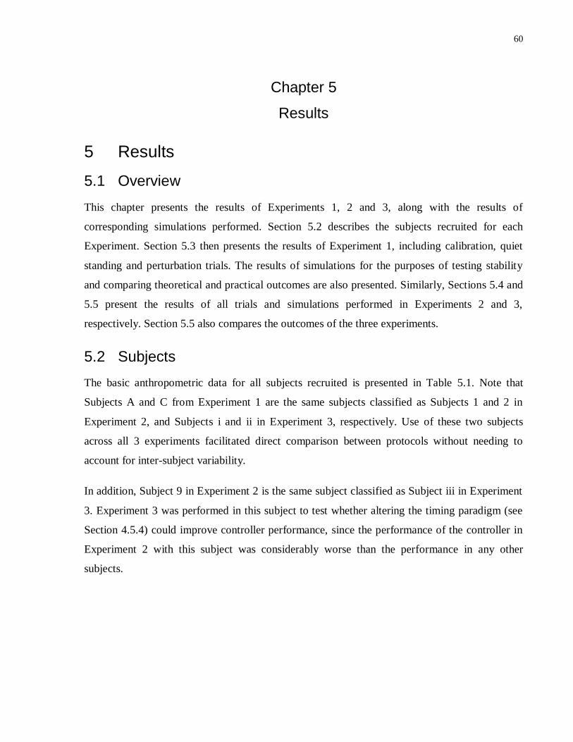
60
Chapter 5
Results
5 Results
5.1 Overview
This chapter presents the results of Experiments 1, 2 and 3, along with the results of
corresponding simulations performed. Section 5.2 describes the subjects recruited for each
Experiment. Section 5.3 then presents the results of Experiment 1, including calibration, quiet
standing and perturbation trials. The results of simulations for the purposes of testing stability
and comparing theoretical and practical outcomes are also presented. Similarly, Sections 5.4 and
5.5 present the results of all trials and simulations performed in Experiments 2 and 3,
respectively. Section 5.5 also compares the outcomes of the three experiments.
5.2 Subjects
The basic anthropometric data for all subjects recruited is presented in Table 5.1. Note that
Subjects A and C from Experiment 1 are the same subjects classified as Subjects 1 and 2 in
Experiment 2, and Subjects i and ii in Experiment 3, respectively. Use of these two subjects
across all 3 experiments facilitated direct comparison between protocols without needing to
account for inter-subject variability.
In addition, Subject 9 in Experiment 2 is the same subject classified as Subject iii in Experiment
3. Experiment 3 was performed in this subject to test whether altering the timing paradigm (see
Section 4.5.4) could improve controller performance, since the performance of the controller in
Experiment 2 with this subject was considerably worse than the performance in any other
subjects.

61
Participants Gender
(M/F)
Age
(years)
Height
(m)
Weight
(kg)
Experiment 1
Subject A M 30 1.70 63
Subject B M 22 1.78 75
Subject C M 32 1.69 75
Experiment 2
Subject 1 M 30 1.70 63
Subject 2 M 32 1.69 75
Subject 3 M 21 1.80 73
Subject 4 M 29 1.80 77
Subject 5 M 23 1.86 83
Subject 6 M 26 1.83 75
Subject 7 F 20 1.57 54
Subject 8 F 25 1.65 63
Subject 9 F 21 1.69 56
Subject 10 F 20 1.70 61
Subject 11 F 24 1.60 67
Experiment 3
Subject i M 30 1.70 65
Subject ii M 32 1.69 75
Subject iii F 21 1.69 56
Table 5.1: Anthropometric data for each subject. The coloured entries connote subjects that were reused
across experiments (i.e., Subjects A, 1 and i represent a single individual who took part in all three
experiments; Subjects C, 2 and ii represent a single individual who took part in all three experiments; and
Subjects 9 and iii represent a single individual who took part in Experiments 2 and 3).
In Experiment 2, a total of 11 subjects were recruited. However, at the conclusion of the
calibration procedure, Subject 10 fainted and was subsequently removed from the study. Subject
11 also complained of dizziness during the calibration procedure and was removed from the
study. These events are believed to have been the result of pre-existing conditions in these
subjects coupled with a prolonged period of stance (15-20 minutes). A third subject (Subject 6)
fainted towards the end of a 5-minute trial, and therefore did not complete the remainder of the
trials. In this case, the fainting spell was believed to have been caused by the disorientating
effects of the proprioceptive and somatosensory information from the ankles, coupled with the
disruption to all other sensory systems. In both fainting situations, there was no risk of falling or
injury to the subjects since the IPSA was supporting the lower limbs. No other adverse events
were observed in any of the experiments.

62
5.3 Experiment 1
5.3.1 Calibration
Muscle recruitment curves were successfully obtained for all 3 subjects. The curves of Subjects
B and C are shown in Figure 5.1, below, whilst Subject A’s recruitment curves are depicted in
Figure 4.7. The maximum torques produced by the plantarflexors (after subtracting the baseline
torque) of Subjects A, B and C were 123 N.m, 108 N.m and 156 N.m, respectively. The
maximum torques produced by the dorsiflexors of Subjects A, B and C were 20.3 N.m, 3.61 N.m
and 27.8 N.m, respectively. These maximum torques were used in saturation blocks during
simulations performed after the experiments.
Figure 5.1: Muscle recruitment curves for the plantarflexors and dorsiflexors of Subjects B and C in
Experiment 1. The blue lines represent the continuous torque recordings during intermittent 5-second
periods of increasing stimulation current amplitude. The maroon markers represent the established torque
values at each FES amplitude, and the maroon lines represent the linear interpolations that were utilized in
between FES amplitudes.
5.3.2 Experimental Trials
Following calibration, an average of 7 short trials was performed in order to tune the controller
gains. In all 3 subjects, establishing appropriate parameters proved to be a relatively straight-
5 10 15 20 25 30 35 40 45 50 55 60
0
50
100
150
0 20 40 60 80 100 120
Current Amplitude (mA)
Torq
ue
(N
m)
Time (seconds)
Subject B - Plantarflexor Recruitment Curve
10 15 20 25 30 35 40 45
2
3
4
5
6
7
0 20 40 60
Current Amplitude (mA)
Torq
ue
(N
m)
Time (seconds)
Subject B - Dorsiflexor Recruitment Curve
10 15 20 25 30 35 40 45 50 55 60
0
50
100
150
200
0 20 40 60 80 100
Current Amplitude (mA)
Torq
ue
(N
m)
Time (seconds)
Subject C - Plantarflexor Recruitment Curve
10 15 20 25 30 35 40 45
-10
-5
0
5
10
15
20
25
0 20 40 60
Current Amplitude (mA)
Torq
ue
(N
m)
Time (seconds)
Subject C - Dorsiflexor Recruitment Curve

63
forward procedure and the performance of the controller was not unduly sensitive to small
variations in parameters. The appropriateness of selecting the same controller parameters for
both plantarflexors and dorsiflexors was also verified. The parameters selected are summarized
in Table 5.2.
KP (Nm / rad) KI (Nm / rad s) KD (Nm s / rad) N (1/s)
Subject A 800 0 0.3125 150
Subject B 350 50 0.714 150
Subject C 350 50 0.714 150
Table 5.2: Controller gains employed in Experiment 1 for both the plantarflexors and dorsiflexors.
In Figure 5.2, inverted pendulum angles during 10-minute quiet standing trials with and without
the closed-loop controlled FES system applied are depicted for each of the 3 subjects. In these
trials, the performance of the PID plus gravity controller during quiet stance compared
favourably with voluntary control as evidenced by mean inverted pendulum angles which were
closer to the reference angle and by lower RMSD values for all subjects (see Table 5.3).
Figure 5.2: Inverted pendulum angles during 10-minute quiet standing trials with the closed-loop controlled
FES system activated shown in blue (FES Condition) and with voluntary control shown in black (Voluntary
Condition with Eyes Closed). (a) Subject A; (b) Subject B; (c) Subject C.
1
3
5
7
9
11
0 200 400 600
An
gle
(d
eg
ree
s)
Time (seconds)
FESVoluntary
(a)
1
3
5
7
9
11
0 200 400 600
An
gle
(d
eg
ree
s)
Time (seconds)
FESVoluntary
(b)
1
3
5
7
9
11
0 200 400 600
An
gle
(d
eg
ree
s)
Time (seconds)
FESVoluntary
(c)
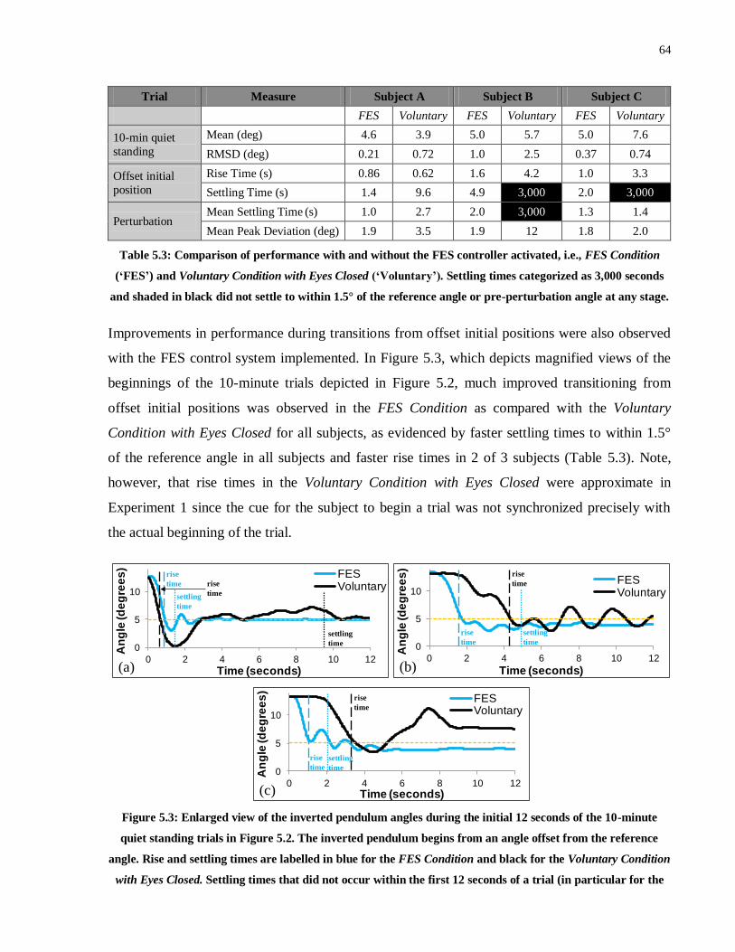
64
Trial Measure Subject A Subject B Subject C
FES Voluntary FES Voluntary FES Voluntary
10-min quiet
standing
Mean (deg) 4.6 3.9 5.0 5.7 5.0 7.6
RMSD (deg) 0.21 0.72 1.0 2.5 0.37 0.74
Offset initial
position
Rise Time (s) 0.86 0.62 1.6 4.2 1.0 3.3
Settling Time (s) 1.4 9.6 4.9 3,000 2.0 3,000
Perturbation Mean Settling Time (s) 1.0 2.7 2.0 3,000 1.3 1.4
Mean Peak Deviation (deg) 1.9 3.5 1.9 12 1.8 2.0
Table 5.3: Comparison of performance with and without the FES controller activated, i.e., FES Condition
(‘FES’) and Voluntary Condition with Eyes Closed (‘Voluntary’). Settling times categorized as 3,000 seconds
and shaded in black did not settle to within 1.5° of the reference angle or pre-perturbation angle at any stage.
Improvements in performance during transitions from offset initial positions were also observed
with the FES control system implemented. In Figure 5.3, which depicts magnified views of the
beginnings of the 10-minute trials depicted in Figure 5.2, much improved transitioning from
offset initial positions was observed in the FES Condition as compared with the Voluntary
Condition with Eyes Closed for all subjects, as evidenced by faster settling times to within 1.5°
of the reference angle in all subjects and faster rise times in 2 of 3 subjects (Table 5.3). Note,
however, that rise times in the Voluntary Condition with Eyes Closed were approximate in
Experiment 1 since the cue for the subject to begin a trial was not synchronized precisely with
the actual beginning of the trial.
Figure 5.3: Enlarged view of the inverted pendulum angles during the initial 12 seconds of the 10-minute
quiet standing trials in Figure 5.2. The inverted pendulum begins from an angle offset from the reference
angle. Rise and settling times are labelled in blue for the FES Condition and black for the Voluntary Condition
with Eyes Closed. Settling times that did not occur within the first 12 seconds of a trial (in particular for the
0
5
10
0 2 4 6 8 10 12
An
gle
(d
eg
ree
s)
Time (seconds)
FESVoluntary
(a)
settling
time
settling
time
rise
time rise
time
0
5
10
0 2 4 6 8 10 12
An
gle
(de
gre
es
)
Time (seconds)
FESVoluntary
(b)
rise
time
settling
time
rise
time
0
5
10
0 2 4 6 8 10 12
An
gle
(d
eg
ree
s)
Time (seconds)
FESVoluntary
(c)
rise
time
settling
time
rise
time

65
Voluntary Condition with Eyes Closed) are not shown. (a) Subject A; (b) Subject B; (c) Subject C.
In Figure 5.4, inverted pendulum angles are depicted for 1-minute trials in the presence of
external, manually applied posterior perturbations of the inverted pendulum in the FES Condition
and Voluntary Condition with Eyes Closed. From these plots, it is evident that the closed-loop
controlled FES system allowed for more rapid and more reliable transitioning towards the
reference angle following perturbations. Decreased mean peak posterior deviations and mean
settling times following perturbations were observed in the FES Condition in all subjects (see
Table 5.3).
Figure 5.4: Inverted pendulum angles during 1-minute trials in which 4 posterior perturbations were applied
at random times. The FES Condition in blue is compared with the Voluntary Condition with Eyes Closed in
black. The arrows represent the perturbation times. (a) Subject A; (b) Subject B; (c) Subject C.
In Figure 5.5, a magnified view of a typical section of the 10-minute quiet standing trial in the
FES Condition for Subject 1 (see Figure 5.2(a)) is depicted in the top plot, whilst the bottom plot
depicts the corresponding plantarflexor and dorsiflexor torques requested and the current
amplitudes applied. Note that the absolute values of the requested torques were used such that all
plots were visible on the positive vertical axis. The exhibited behaviour (small oscillations in the
inverted pendulum angle, low but mostly non-zero and gradually fluctuating levels of current
applied to the plantarflexors, and only brief, intermittent activation of the dorsiflexors) was
commonly observed across multiple trials and across all 3 subjects.
-2
0
2
4
6
8
10
12
0 20 40 60
An
gle
(d
eg
ree
s)
Time (seconds)
FES
Voluntary
= Perturbation(Voluntary)
= Perturbation
(FES)(a)
-2
0
2
4
6
8
10
12
0 20 40 60A
ng
le (d
eg
ree
s)
Time (seconds)
FES
Voluntary
= Perturbation(Voluntary)
= Perturbation(FES)
(b)
-2
0
2
4
6
8
10
12
0 20 40 60
An
gle
(d
eg
ree
s)
Time (seconds)
FESVoluntary
= Perturbation(Voluntary)
= Perturbation
(FES)(c)

66
Figure 5.5: Top: Inverted pendulum angle during 15 seconds of the 10-minute quiet standing trial with the
FES controller activated (FES Condition) for Subject 1. Bottom: The corresponding plantarflexor and
dorsiflexor currents, and requested plantarflexor and dorsiflexor torques (PF = plantarflexor; DF =
dorsiflexor).
Due to the fact that the same controller parameters were found to be appropriate for Subjects B
and C, some subsequent short trials were performed in Subject A at these same parameters to test
the potential of the controller at standardized parameters. The controller also performed well at
these parameters in Subject A. A 12-second trial testing ability to overcome an offset initial
position is shown in Figure 5.6. Given that a much lower proportional gain was used as
compared with the trial depicted in Figure 5.3(a), it is not surprising that a longer rise time was
observed. However, importantly, the inverted pendulum was reliably maintained about the
reference angle. This result adds weight to the notion that Controller A could potentially be
sufficiently robust in this paradigm to allow standardized parameters to be employed
0
5
10
15
20
25
30
0
5
10
15
20
25
30
35
40
415 420 425 430
Req
ueste
d T
orq
ue (
Nm
)
Cu
rren
t (m
A)
Time (seconds)
PF Current DF Current
Requested PF Torque Requested DF Torque
4
4.5
5A
ng
le (
deg
rees)
Pendulum Angle
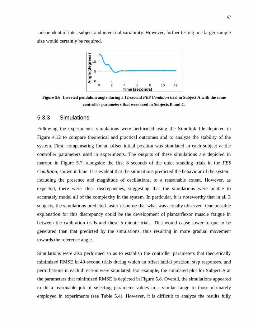
67
independent of inter-subject and inter-trial variability. However, further testing in a larger sample
size would certainly be required.
Figure 5.6: Inverted pendulum angle during a 12-second FES Condition trial in Subject A with the same
controller parameters that were used in Subjects B and C.
5.3.3 Simulations
Following the experiments, simulations were performed using the Simulink file depicted in
Figure 4.12 to compare theoretical and practical outcomes and to analyze the stability of the
system. First, compensating for an offset initial position was simulated in each subject at the
controller parameters used in experiments. The outputs of these simulations are depicted in
maroon in Figure 5.7, alongside the first 8 seconds of the quiet standing trials in the FES
Condition, shown in blue. It is evident that the simulations predicted the behaviour of the system,
including the presence and magnitude of oscillations, to a reasonable extent. However, as
expected, there were clear discrepancies, suggesting that the simulations were unable to
accurately model all of the complexity in the system. In particular, it is noteworthy that in all 3
subjects, the simulations predicted faster response that what was actually observed. One possible
explanation for this discrepancy could be the development of plantarflexor muscle fatigue in
between the calibration trials and these 5-minute trials. This would cause lower torque to be
generated than that predicted by the simulations, thus resulting in more gradual movement
towards the reference angle.
Simulations were also performed so as to establish the controller parameters that theoretically
minimized RMSE in 40-second trials during which an offset initial position, step responses, and
perturbations in each direction were simulated. For example, the simulated plot for Subject A at
the parameters that minimized RMSE is depicted in Figure 5.8. Overall, the simulations appeared
to do a reasonable job of selecting parameter values in a similar range to those ultimately
employed in experiments (see Table 5.4). However, it is difficult to analyze the results fully
0
5
10
0 2 4 6 8 10 12
An
gle
(d
eg
ree
s)
Time (seconds)

68
since the simulations were only performed post-experimentation and, as a result, experiments
were not performed at the precise parameters suggested from the simulations.
Figure 5.7: Enlarged view of the inverted pendulum angles during the initial 8 seconds of the 10-minute quiet
standing trials shown in Figure 5.2. The results of experiments in blue (FES Condition) are compared with the
results of simulations using the same controller parameters in maroon (a) Subject A; (b) Subject B; (c)
Subject C.
Figure 5.8: Simulation of inverted pendulum angle (in blue) for Subject 1 at the controller parameters that
minimized RMSE. The orange plot represents the reference angle. The simulation includes an offset initial
position, a step response from 5° to 9° (t = 10 s to 18 s), and anterior (t = 25 s) and posterior (t = 32 s)
perturbations.
The large difference between the results for Subject B compared with Subjects A and C (see
Table 5.4) suggests that the simulation output was highly sensitive to changes in maximum
0
5
10
0 2 4 6 8
An
gle
(d
eg
ree
s)
Time (seconds)
Experiment
Simulation
(a)
0
5
10
0 2 4 6 8
An
gle
(de
gre
es
)
Time (seconds)
Experiment
Simulation
(b)
0
5
10
0 2 4 6 8
An
gle
(d
eg
ree
s)
Time (seconds)
Experiment
Simulation
(c)
0 10 20 30 402
4
6
8
10
12
14
Angle
(degre
es)
Time (seconds)
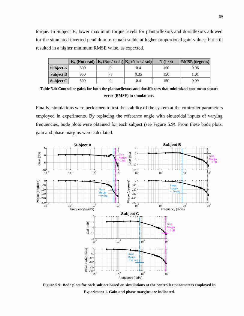
69
torque. In Subject B, lower maximum torque levels for plantarflexors and dorsiflexors allowed
for the simulated inverted pendulum to remain stable at higher proportional gain values, but still
resulted in a higher minimum RMSE value, as expected.
KP (Nm / rad) KI (Nm / rad s) KD (Nm s / rad) N (1 / s) RMSE (degrees)
Subject A 500 0 0.4 150 0.96
Subject B 950 75 0.35 150 1.01
Subject C 500 0 0.4 150 0.99
Table 5.4: Controller gains for both the plantarflexors and dorsiflexors that minimized root mean square
error (RMSE) in simulations.
Finally, simulations were performed to test the stability of the system at the controller parameters
employed in experiments. By replacing the reference angle with sinusoidal inputs of varying
frequencies, bode plots were obtained for each subject (see Figure 5.9). From these bode plots,
gain and phase margins were calculated.
Figure 5.9: Bode plots for each subject based on simulations at the controller parameters employed in
Experiment 1. Gain and phase margins are indicated.
10-2
10-1
100
101
-10
-5
0
5
Ga
in (
dB
)
Subject A
10-2
10-1
100
101
-300
-240
-180
-120
-60
0
Frequency (rad/s)
Ph
ase
(d
eg
ree
s)
Gain Margin~3 dB
Phase Margin~40 deg
10-2
10-1
100
101
-15
-10
-5
0
5
Ga
in (
dB
)
Subject B
10-2
10-1
100
101
-300
-240
-180
-120
-60
0
Frequency (rad/s)
Ph
ase
(d
eg
ree
s)
Gain Margin~10 dB
Phase Margin~150 deg
10-2
10-1
100
101
-15
-10
-5
0
5
Ga
in (
dB
)
Subject C
10-2
10-1
100
101
-300
-240
-180
-120
-60
0
Frequency (rad/s)
Ph
ase
(d
eg
ree
s)
Phase Margin~150 deg
Gain Margin~10 dB

70
If either the gain or phase margin falls below zero, this is indicative of instability. In addition,
larger positive gain and phase margins are typically suggestive of enhanced robustness in terms
of stability, and a common rule of thumb is that acceptable gain and phase margins should have
values of at least 3 dB and 60°, respectively. These criteria have been employed in multiple
studies examining PID controller tuning procedures108,109
. Thus, in this dissertation, if either of
these criteria were not met (but gain and phase margins were both above zero), the system was
defined as marginally stable, but if both criteria were met then the system was defined as stable.
From the bode plots above, it is evident that all gain and phase margins were positive and met the
criteria, suggesting that the system was stable for all 3 subjects at the parameters employed
(although Subject A is on the cusp). It is not surprising that the gain and phase margins were
lowest for Subject 1 given the much larger proportional gains employed for this subject.
5.4 Experiment 2
5.4.1 Calibration
Calibration was successfully performed in all 9 subjects. Note that Subject 10 also successfully
completed the calibration procedure but since no trials were performed, the results have not been
included. Subjects 1-6 were all stimulated over the full range of FES amplitudes (up to 60 mA
for plantarflexors and 45 mA for dorsiflexors). Subjects 7-9 complained of discomfort at higher
FES amplitudes. Therefore, Subjects 7, 8 and 9 received maximum amplitudes (during
calibration and experimental trials) of 45 mA, 45 mA, and 55 mA, respectively, for the
plantarflexors; and 35 mA, 30 mA and 40 mA for the dorsiflexors, respectively.
In all subjects and for both the plantarflexors and dorsiflexors, the sinusoidally varying FES
amplitudes yielded torque values that varied approximately sinusoidally at the same frequencies
as the inputs. Thus, sinusoidal curves of best fit could be reliably applied to calculate phase delay
and gain (as shown in Figures 4.9 and 4.10 for Subject 1). The plots for all other subjects are
depicted in Appendix B.
From the calculated phase and gain information, first order models were established for each
subject and muscle group, as depicted by the solid blue lines in the bode plots shown in Figure
5.10. The actual calculated gain and phase values are marked by black crosses. From these plots,
it is evident that the first order models were able to match the measured data quite reliably.

71
Nonetheless, there were some discrepancies between the measured data and the first order
models. Whilst the models were generally very accurate at predicting gain values, there was
typically less agreement in terms of phase values. In particular, for most subjects, at the lower
frequencies tested, the measured phase lag exceeded the phase lag suggested by the first order
models. By definition, the phase lag in a first order model will tend to 0° as the frequency tends
to zero, but the measured data appears to indicate the presence of a constant delay that remained
even at very low frequencies. This result was somewhat surprising given the magnitude of this
delay in some subjects and the fact that a 100 ms delay had already been removed from the phase
lag calculations. This 100 ms delay was factored in so as to match the constant delay between the
onset of FES and torque beginning to be generated during step response trials (as in the
calibration for Experiment 1). Since this constant delay prior to the onset of torque generation
was found experimentally to be in the vicinity of 100 ms, no additional constant delays were
added despite the differences observed between phase values obtained experimentally and those
predicted by the first order model.
It is likely that non-linearities in muscle behaviour could have resulted in varying muscle
dynamics in response to step and sinusoidal inputs. In fact, Ferrarin and Pedotti110
created first-
order models of knee extensor muscle dynamics in response to FES, but found that the models
exhibited significantly larger delays when created based on a ramp input as opposed to a step
input. This would explain why larger delays appeared to be present in response to low frequency
sinusoidally varying inputs as opposed to step inputs. If this is the case, then a single first order
model may struggle to encapsulate muscle behaviour in response to FES waveforms fluctuating
at different frequencies.
The additional delays observed could also have partly been a product of the experimental design.
In particular, the calibration procedure assumed a linear relationship between FES amplitude and
torque. However, as evidenced by the calibration curves in Experiment 1, the relationship is not
actually linear, particularly at lower FES amplitudes. As a result, the torque curves obtained were
not exactly sinusoidal. For example, since the FES amplitude sinusoidally increased from 20
mA, there was often a delay prior to torque increasing appreciably, which could have presented
itself as a constant delay at low frequencies.
It should also be noted that frequency domain analyses of quiet stance in able-bodied subjects
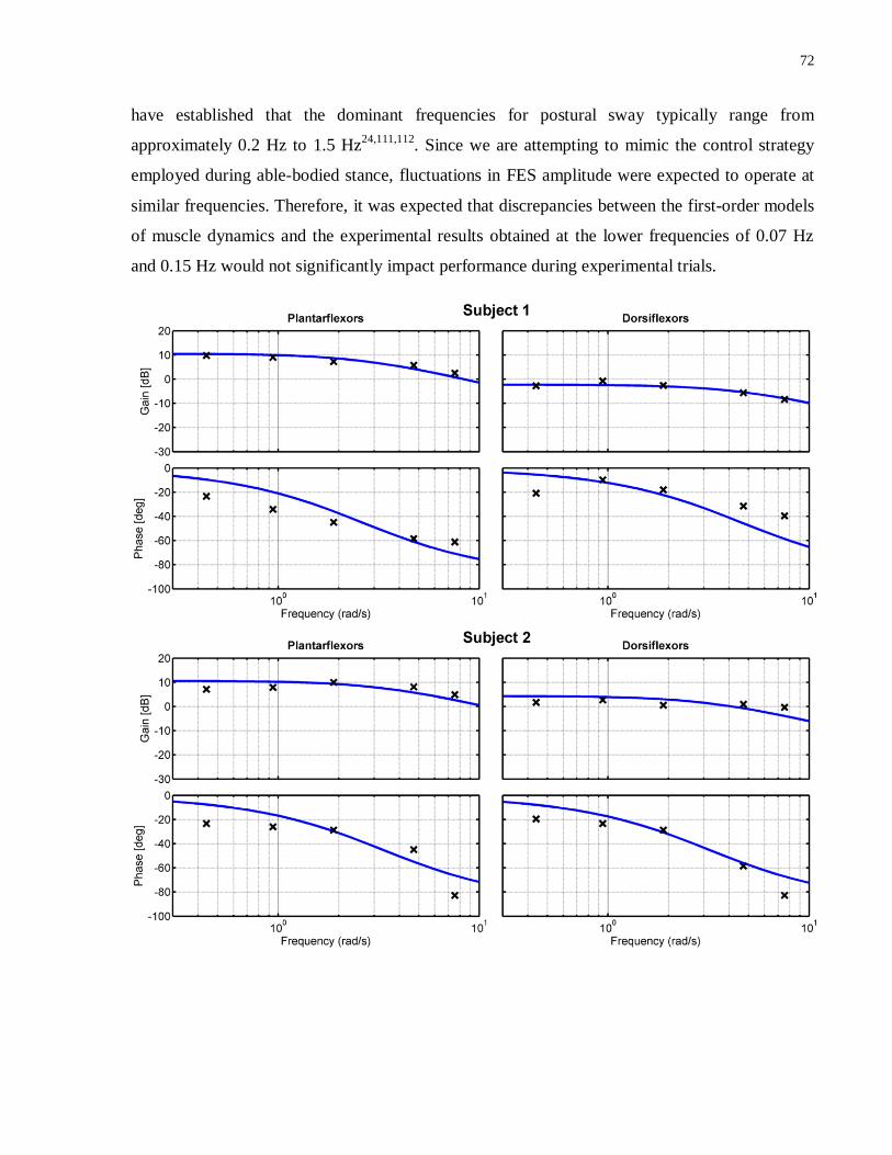
72
have established that the dominant frequencies for postural sway typically range from
approximately 0.2 Hz to 1.5 Hz24,111,112
. Since we are attempting to mimic the control strategy
employed during able-bodied stance, fluctuations in FES amplitude were expected to operate at
similar frequencies. Therefore, it was expected that discrepancies between the first-order models
of muscle dynamics and the experimental results obtained at the lower frequencies of 0.07 Hz
and 0.15 Hz would not significantly impact performance during experimental trials.
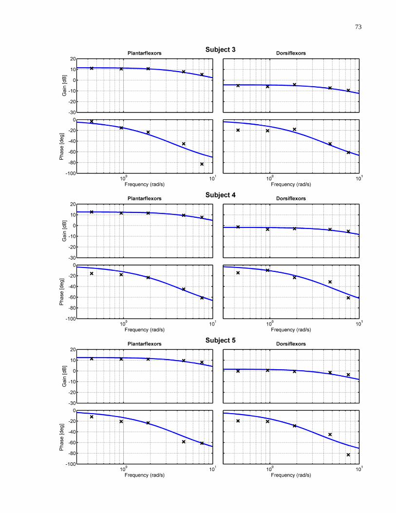
73
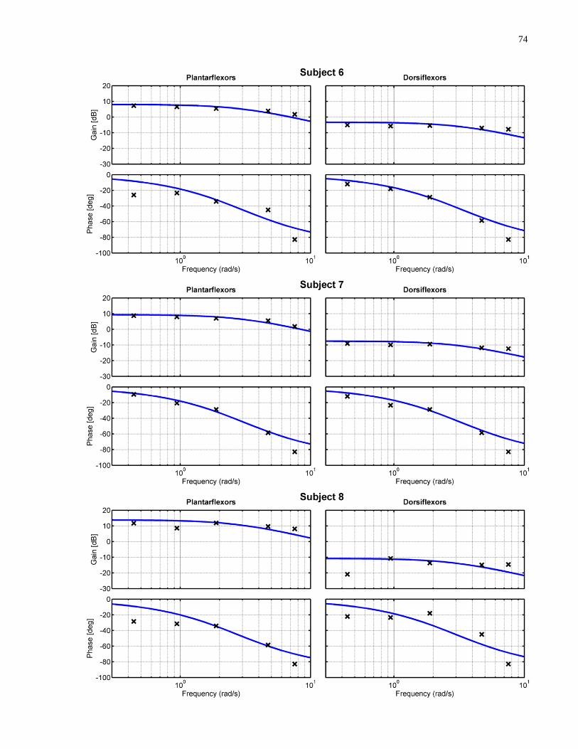
74

75
Figure 5.10: Bode plots depicting phase and amplitude response data obtained experimentally (black crosses),
and corresponding bode plots from the first order muscle dynamics transfer functions calculated (solid blue
lines) for Subjects 1-9.
The K and α-values (see Equation 4.6) obtained for each subject and muscle group are presented
in Table 5.5. The K-values, which are representative of the gains between FES amplitude and
torque, varied between 2.53 and 4.90 for the plantarflexors, and between 0.29 and 1.65 for the
dorsiflexors. These results verify that there exists large variability in sensitivity to FES and
torque generation ability. Similarly, there was considerable variation in terms of α (0.23 – 0.38
for plantarflexors; 0.19 – 0.32 for dorsiflexors). Since α is representative of the dynamics of
muscle response to FES, this apparent variability is an important consideration, and provides
justification for the use of these first order models (as opposed to Experiment 1, in which
transient behaviour was not considered).
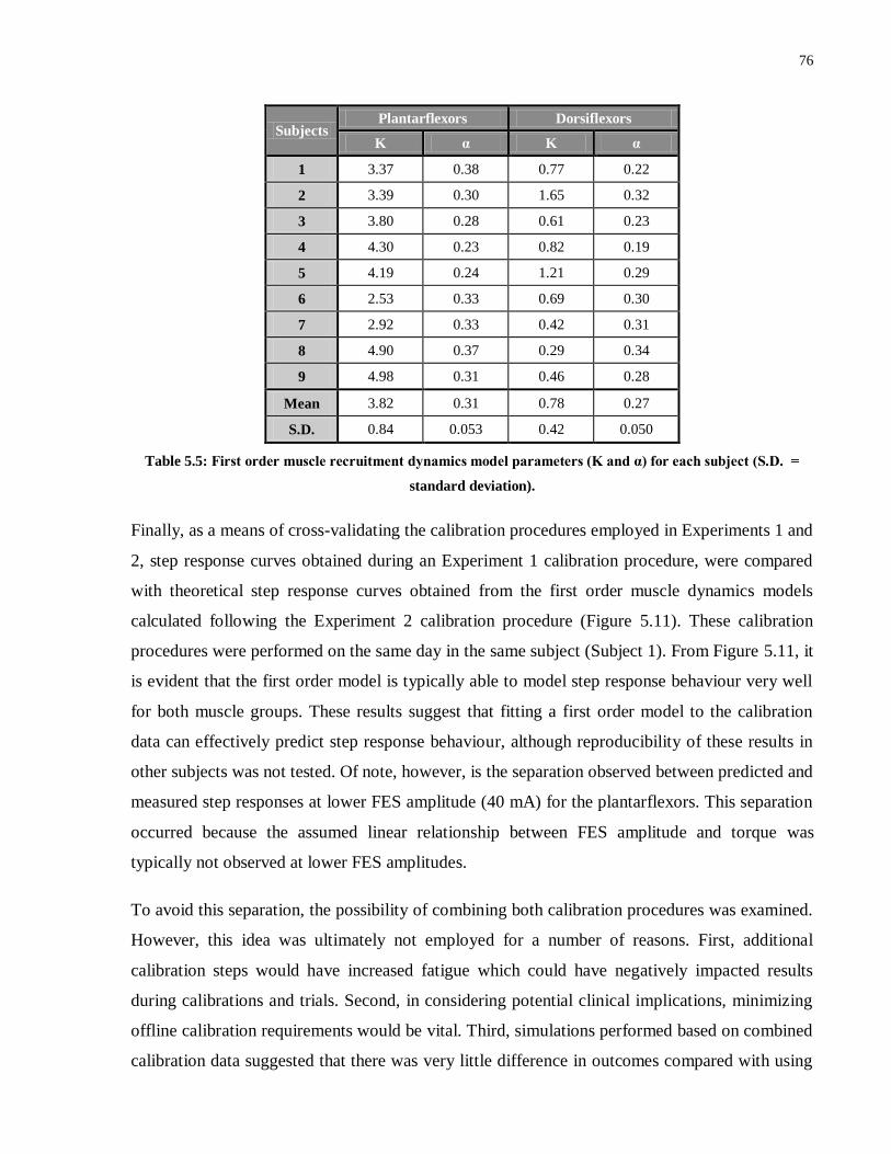
76
Subjects Plantarflexors Dorsiflexors
K α K α
1 3.37 0.38 0.77 0.22
2 3.39 0.30 1.65 0.32
3 3.80 0.28 0.61 0.23
4 4.30 0.23 0.82 0.19
5 4.19 0.24 1.21 0.29
6 2.53 0.33 0.69 0.30
7 2.92 0.33 0.42 0.31
8 4.90 0.37 0.29 0.34
9 4.98 0.31 0.46 0.28
Mean 3.82 0.31 0.78 0.27
S.D. 0.84 0.053 0.42 0.050
Table 5.5: First order muscle recruitment dynamics model parameters (K and α) for each subject (S.D. =
standard deviation).
Finally, as a means of cross-validating the calibration procedures employed in Experiments 1 and
2, step response curves obtained during an Experiment 1 calibration procedure, were compared
with theoretical step response curves obtained from the first order muscle dynamics models
calculated following the Experiment 2 calibration procedure (Figure 5.11). These calibration
procedures were performed on the same day in the same subject (Subject 1). From Figure 5.11, it
is evident that the first order model is typically able to model step response behaviour very well
for both muscle groups. These results suggest that fitting a first order model to the calibration
data can effectively predict step response behaviour, although reproducibility of these results in
other subjects was not tested. Of note, however, is the separation observed between predicted and
measured step responses at lower FES amplitude (40 mA) for the plantarflexors. This separation
occurred because the assumed linear relationship between FES amplitude and torque was
typically not observed at lower FES amplitudes.
To avoid this separation, the possibility of combining both calibration procedures was examined.
However, this idea was ultimately not employed for a number of reasons. First, additional
calibration steps would have increased fatigue which could have negatively impacted results
during calibrations and trials. Second, in considering potential clinical implications, minimizing
offline calibration requirements would be vital. Third, simulations performed based on combined
calibration data suggested that there was very little difference in outcomes compared with using
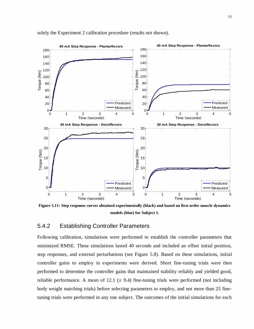
77
solely the Experiment 2 calibration procedure (results not shown).
Figure 5.11: Step response curves obtained experimentally (black) and based on first order muscle dynamics
models (blue) for Subject 1.
5.4.2 Establishing Controller Parameters
Following calibration, simulations were performed to establish the controller parameters that
minimized RMSE. These simulations lasted 40 seconds and included an offset initial position,
step responses, and external perturbations (see Figure 5.8). Based on these simulations, initial
controller gains to employ in experiments were derived. Short fine-tuning trials were then
performed to determine the controller gains that maintained stability reliably and yielded good,
reliable performance. A mean of 12.1 (± 9.4) fine-tuning trials were performed (not including
body weight matching trials) before selecting parameters to employ, and not more than 25 fine-
tuning trials were performed in any one subject. The outcomes of the initial simulations for each
0 1 2 3 4 50
20
40
60
80
100
120
140
160
180
Time (seconds)
Torq
ue (
Nm
)
60 mA Step Response - Plantarflexors
Predicted
Measured
0 1 2 3 4 50
20
40
60
80
100
120
140
160
180
Time (seconds)
Torq
ue (
Nm
)
40 mA Step Response - Plantarflexors
Predicted
Measured
0 1 2 3 4 5
0
5
10
15
20
25
30
Time (seconds)
Torq
ue (
Nm
)
45 mA Step Response - Dorsiflexors
Predicted
Measured
0 1 2 3 4 5
0
5
10
15
20
25
30
Time (seconds)
Torq
ue (
Nm
)
30 mA Step Response - Dorsiflexors
Predicted
Measured
78
subject are depicted in Table 5.6 alongside the gains ultimately employed following experimental
fine-tuning. The controller parameters that minimized RMSE in simulations performed post-
experimentation using an updated Simulink file (see Figure 4.14) are also shown.
Despite some deficiencies in the initial simulation protocol, the simulations performed
reasonably and were typically able to suggest gains that were ultimately in close proximity to the
gains employed in experiments. Note that the controller gains that minimized RMSE in the initial
simulations were reduced by 25% in order to enhance stability, as discussed in Section 4.4.2.1.
The reduced gains are listed on the left hand side of Table 5.6, although the stated RMSE values
correspond to the minimized RMSEs calculated with the larger gains.
In 3 subjects, the parameters suggested in simulations were identical to those ultimately
employed during the 5-minute quiet standing trial. However, in Subject 3, the controller
parameters were altered again following the 5-minute trials (to KP = 160, KD = 0.56, KI = 5) so
as to improve stability in the step response trials. In 2 other subjects, one of the three controller
gain values had to be adjusted; in 1 subject, two gain values had to be changed; and in 1 subject,
all 3 values had to be changed. In Subjects 8 and 9, additional challenges were encountered
(discussed below).
As shown in Table 5.6, the initial simulations appeared to perform particularly well for body
weight matching trials, with each of the 4 subjects that completed the body weight matching
experiments retaining the controller gains suggested by the simulations. However, this result may
have been a consequence of a shorter fine-tuning protocol. Since a maximum of 5 fine-tuning
trials were performed, so as to minimize fatigue, it was not possible to ascertain fully the most
appropriate parameters.
Whilst the initial simulations performed reasonably overall, there were some limitations. First
and foremost, at almost all gain values and for both the regular and body weight matching
simulations, sizeable oscillations were observed throughout trials. The presence of these
oscillations is verified by much larger RMSE values when compared with post-experimentation
simulations. These oscillations were believed to be a result of the method employed to model the
switching between muscles, and were likely exacerbated (in comparison with the simulations
performed post-experimentation) by larger constant delay values, and the lack of passive and
voluntary components in the simulations. As a consequence of these oscillations, performance

79
and stability was heavily contingent on position within an oscillatory period at the time of step
responses and perturbations. As a result, small changes in controller gains could impact heavily
on the RMSE values obtained, as well as the ability to maintain stability, thus adversely affecting
ability to reliably yield appropriate gain values. A further limitation was that larger derivative
gains were suggested from the simulations compared with those that provided the best
experimental results. Since the derivative gain term was already expressed as a fraction of the
proportional gain, reducing both the derivative and proportional gains by 25% actually reduced
the derivative contribution by 50%. Since the updated model used post-experimentation
overcame these issues, further discussion of the initial simulation technique is not provided.
In the post-experimentation simulations, the voluntary gain (V) was set to 65 Nm/rad, whilst the
stiffness gain (K) was set to 90 Nm/rad for the regular trials and 300 Nm/rad for the body weight
matching trials. These values were assigned based on comparisons between simulations and
experimental results (see Section 5.4.4). Importantly, these stiffness gain values were also in
agreement with those suggested in previous studies. In particular, Fitzpatrick et al113
utilized an
inverted pendulum device very similar to the IPSA, with weight added to the inverted pendulum
to approximately match the subject’s body weight. They calculated ankle stiffness in 5 subjects
using this device by analyzing the relationship between torque and inverted pendulum angle, and
obtained values that varied from approximately 200 Nm/rad to 400 Nm/rad with an average in
the vicinity of 300 Nm/rad. It is logical that stiffness would be lower when less weight was
added to the inverted pendulum.
It is difficult to ascertain the effectiveness of the post-experimentation simulations for selecting
gains given that the suggested parameters were not tested directly. Since the fine-tuning trials
were not exhaustive, it is possible that these suggested parameters could in fact have yielded
improved performance. Nonetheless, some interesting observations can be extracted. First, these
simulations suggested controller gains that were typically in the vicinity of those ultimately
employed. For the most part, the proportional gains suggested were higher than those employed
in experiments, although this is to be expected given that the goal of the simulations was to
minimize RMSE and not to maximize stability. Furthermore, these proportional gains were not
reduced by any factor as they were for the initial simulations. The derivative gains, on the other
hand, appeared more reasonable than in the initial simulations. In fact, they were generally
slightly lower than those obtained in the initial simulations even after those gains were reduced.

80
Interestingly, in the body weight matching paradigm, slightly higher derivative and integral gains
were suggested. Another important observation was that examination of variations in RMSE
values during each individual simulation protocol yielded more subtle, less erratic changes in
RMSE values in response to minor controller gain variations.
Subject Initial Simulations Experiments Simulations Post-
Experimentation
Kp
(mA /
rad)
Kd
(mA /
rad s)
Ki
(mA s
/ rad)
RMSE
(degs)
Kp
(mA /
rad)
Kd
(mA /
rad s)
Ki
(mA s
/ rad)
Kp
(mA /
rad)
Kd
(mA /
rad s)
Ki
(mA s
/ rad)
RMSE
(degs)
1 203 0.49 25 1.60 203 0.49 25 200 0.45 0 1.46
2 113 0.49 75 1.98 113 0.6 75 160 0.4 50 1.46
3a 120 0.56 75 1.79 120 0.56 75 190 0.45 0 1.37
4 100 0.49 25 1.90 170 0.2 38 150 0.4 25 1.28
5 97.5 0.49 25 1.96 97.5 0.49 25 160 0.4 25 1.31
6 195 0.45 38 1.86 165 0.45 25 230 0.45 25 1.49
7 82.5 0.60 25 2.05 130 0.7 5 290 0.5 25 1.69
8b -- -- -- -- 80 0.8 25 -- -- -- --
9c 120 0.56 38 1.74 -- -- -- 150 0.6 25 1.46
Mean 129 0.52 41 1.86 143 0.50 38 191 0.46 22 1.44
Body Weight Matching Simulations and Experiments:
1 218 0.53 38 2.51 218 0.53 38 270 0.75 50 1.62
3 143 0.5 13 2.31 143 0.5 13 260 0.6 50 1.57
4 158 0.38 25 1.31d 158 0.38 25 280 0.5 50 0.99d
5 173 0.45 25 1.37d 173 0.45 25 310 0.5 50 1.03d
a Parameters were changed to KP = 160, KD = 0.56, KI = 5 following the 5-minute trial. b Control design was altered in Subject 8, so simulations were not performed.
c In experiments in Subject 9, the inverted pendulum could not be stabilized effectively at any controller gains tested. d RMSE values were lower due to the inverted pendulum beginning from 10° rather than 14°.
Table 5.6: Controller gains suggested from simulations performed prior to experiments (left), the gains
ultimately employed in experiments (centre) and the gains suggested based on simulations post-
experimentation using an updated model (right). The gains suggested and employed in regular trials and
body weight matched trials are shown.
5.4.2.1 Challenging Subjects
In Subject 8, the minimum allowable current amplitude had to be reduced in order to achieve
stability. Subject 8’s plantarflexors were unusually sensitive to FES, even at very low
amplitudes, which resulted in considerable torque being generated at the minimum allowable
FES amplitude of 20 mA. This resulted in a propensity for the inverted pendulum to overshoot to
a large extent, crossing the vertical and often becoming unstable, as shown in Figure 5.12. There

81
are a number of reasons why the normal controller design was ill-equipped to provide stability
with this subject:
i. In the trial shown in Figure 5.12, even though the current amplitude only reached a
maximum value marginally above 30 mA, this current level was sufficient to overcome
gravity and rapidly bring the inverted pendulum from 14° towards the reference angle. In
other subjects, the current amplitude required to lift the inverted pendulum was typically
above 40 mA. Given that the amount of torque required to compensate for gravity about the
reference angle is much lower than that at 14°, current amplitudes considerably less than 30
mA would likely have been required during ‘steady state’ operation. However, since the
minimum allowable current level (before the current applied to the plantarflexors drops to 0
mA) was 20 mA this allowed only a very small range for the controller to operate in, which
is particularly problematic given the 1 mA minimum step size of the Compex stimulator.
Moreover, it appears likely that the torque produced at 20 mA would have exceeded the
torque due to gravity at 5°, which would mean that the inverted pendulum would never have
been able to stabilize at a constant 5°.
ii. Since a linear relationship between FES amplitude and torque generated was assumed, the
higher sensitivity to lower FES amplitudes in Subject 8 was not fully accounted for in the
first-order muscle dynamics models. This resulted in the initial simulations suggesting a
proportional gain for the plantarflexors well in excess of the gains that ultimately yielded the
most promising results. (In Figure 5.12, a proportional gain of only 30 was applied.)
Furthermore, since the inverse of the muscle dynamics transfer function was used to convert
the torque due to gravity at the reference angle to a required FES amplitude, a constant
current amplitude in excess of that required was added to the controller throughout.
iii. Subject 8 had the lowest dorsiflexor torque production of all subjects due largely to a
maximum amplitude permitted by the subject of 30 mA. This meant that when the inverted
pendulum overshot the reference angle, the ability of the dorsiflexors to stabilize the system
was limited.
Whilst all of these issues appeared to be minor when subjects’ muscles exhibited small
deviations from the norm, when behaviour was unusual, problems arose, particularly due to the
large hardware and software-induced delays in the system. To overcome the issue in Subject 8,
the controller was adjusted such that 10 mA was added to the real-time required current

82
amplitude instead of 20 mA. This allowed for currents between 10 mA and 20 mA to be
included, and also meant that the constant gravity term became less dominant; both of which
assisted in facilitating stability. Due to this controller adjustment, the parameters used in
simulations and experiments in Subject 8 could not be directly compared with those used in other
subjects. As a result, the simulation results are not shown for Subject 8.
Figure 5.12: The beginning of an FES Condition trial in Subject 8 with the inverted pendulum beginning from
an offset initial position. The real-time inverted pendulum angle (blue) is shown, as well as the plantarflexor
(grey) and dorsiflexor (green) currents.
Finally, in Subject 9, ability to compensate for an offset initial position could not be reliably
obtained, even after fine-tuning. Unlike Subject 8, Subject 9 did not produce considerable torque
at low current amplitudes, but was very sensitive to small fluctuations in current amplitude above
approximately 35 mA. Figure 5.13 depicts an example of a typical trial. Of note, a maximum
current amplitude of approximately 45 mA was initially sufficient to lift the inverted pendulum.
However, then when the current dropped only slightly to 39 mA, the torque generated was
insufficient to maintain the inverted pendulum’s momentum in the anterior direction and the
inverted pendulum began to move posteriorly, even though the torque required to maintain the
inverted pendulum at the new angle of approximately 8° would have been much less. This degree
of sensitivity to small changes in FES amplitudes was not observed in any other subjects. Due to
an inability to maintain stability reliably when overcoming an offset initial position, none of the
longer trials could be performed in Subject 9. However, in Experiment 3 this subject was retested
with the superior timing protocol (see Section 5.5).
0
0.2
0.4
0.6
0.8
1
0 1 2 3 4
2
4
6
8
10
12
14Subject 8 - Fine-Tuning Trial
Angle
(degre
es)
Time (seconds)
0 1 2 3 40
10
20
30
40
50
60
Curr
ent A
mplit
ude (
mA
)
Angle
PF Current
DF Current

83
Figure 5.13: The beginning of an FES Condition trial in Subject 9 with the inverted pendulum beginning from
an offset initial position. The real-time inverted pendulum angle (blue) is shown, as well as the plantarflexor
(grey) and dorsiflexor (green) currents.
5.4.3 Quiet Standing
Following successful completion of fine-tuning trials, 5-minute quiet standing trials were
performed in Subjects 1-8 (Figure 5.14). In Figure 5.14, each set of axes compares the inverted
pendulum angle over time for each subject with the FES controller activated (FES Condition) in
blue and with voluntary control and no FES applied (Voluntary Condition with Eyes Closed) in
black. The 5° reference angle is represented by orange dashed lines.
Importantly, in all 8 subjects the FES controller was able to maintain the inverted pendulum
within the allowable range, thus signifying that stability was reliably achieved. There was also no
evidence of voluntary control being initiated at any stage during trials to stabilize the system or
to avoid the inverted pendulum reaching the endpoints of the allowable range. Note that Subject
6 complained of dizziness with approximately 20 seconds remaining in the 5-minute trial and
therefore the FES was switched off prematurely. When the FES was switched off, the inverted
pendulum returned to its initial position, as shown in Figure 5.14. When calculating performance
metrics such as RMSE for Subject 6, this final 20-second period was included so as to model the
worst-case scenario and to allow easier comparison between subjects and conditions.
0
0.2
0.4
0.6
0.8
1
0 1 2 3 4 5
2
4
6
8
10
12
14Subject 9
Angle
(degre
es)
Time (seconds)
0 1 2 3 4 50
10
20
30
40
50
60
Curr
ent A
mplit
ude (
mA
)
Angle
PF Current
DF Current
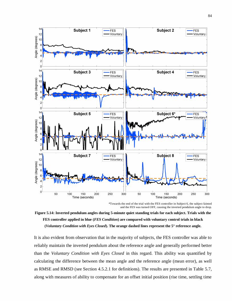
84
*Towards the end of the trial with the FES controller in Subject 6, the subject fainted
and the FES was turned OFF, causing the inverted pendulum angle to drop.
Figure 5.14: Inverted pendulum angles during 5-minute quiet standing trials for each subject. Trials with the
FES controller applied in blue (FES Condition) are compared with voluntary control trials in black
(Voluntary Condition with Eyes Closed). The orange dashed lines represent the 5° reference angle.
It is also evident from observation that in the majority of subjects, the FES controller was able to
reliably maintain the inverted pendulum about the reference angle and generally performed better
than the Voluntary Condition with Eyes Closed in this regard. This ability was quantified by
calculating the difference between the mean angle and the reference angle (mean error), as well
as RMSE and RMSD (see Section 4.5.2.1 for definitions). The results are presented in Table 5.7,
along with measures of ability to compensate for an offset initial position (rise time, settling time
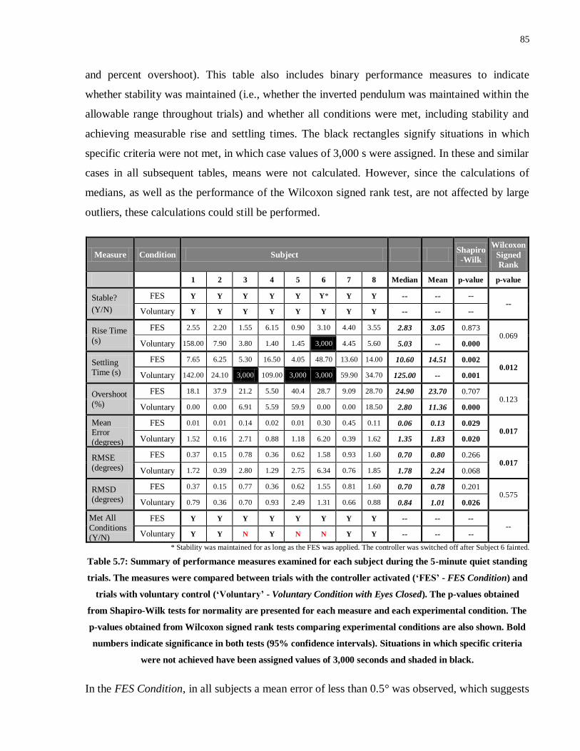
85
and percent overshoot). This table also includes binary performance measures to indicate
whether stability was maintained (i.e., whether the inverted pendulum was maintained within the
allowable range throughout trials) and whether all conditions were met, including stability and
achieving measurable rise and settling times. The black rectangles signify situations in which
specific criteria were not met, in which case values of 3,000 s were assigned. In these and similar
cases in all subsequent tables, means were not calculated. However, since the calculations of
medians, as well as the performance of the Wilcoxon signed rank test, are not affected by large
outliers, these calculations could still be performed.
Measure Condition Subject Shapiro
-Wilk
Wilcoxon
Signed
Rank
1 2 3 4 5 6 7 8 Median Mean p-value p-value
Stable?
(Y/N)
FES Y Y Y Y Y Y* Y Y -- -- -- --
Voluntary Y Y Y Y Y Y Y Y -- -- --
Rise Time
(s)
FES 2.55 2.20 1.55 6.15 0.90 3.10 4.40 3.55 2.83 3.05 0.873 0.069
Voluntary 158.00 7.90 3.80 1.40 1.45 3,000 4.45 5.60 5.03 -- 0.000
Settling Time (s)
FES 7.65 6.25 5.30 16.50 4.05 48.70 13.60 14.00 10.60 14.51 0.002 0.012
Voluntary 142.00 24.10 3,000 109.00 3,000 3,000 59.90 34.70 125.00 -- 0.001
Overshoot
(%)
FES 18.1 37.9 21.2 5.50 40.4 28.7 9.09 28.70 24.90 23.70 0.707 0.123
Voluntary 0.00 0.00 6.91 5.59 59.9 0.00 0.00 18.50 2.80 11.36 0.000
Mean Error (degrees)
FES 0.01 0.01 0.14 0.02 0.01 0.30 0.45 0.11 0.06 0.13 0.029 0.017
Voluntary 1.52 0.16 2.71 0.88 1.18 6.20 0.39 1.62 1.35 1.83 0.020
RMSE
(degrees)
FES 0.37 0.15 0.78 0.36 0.62 1.58 0.93 1.60 0.70 0.80 0.266 0.017
Voluntary 1.72 0.39 2.80 1.29 2.75 6.34 0.76 1.85 1.78 2.24 0.068
RMSD (degrees)
FES 0.37 0.15 0.77 0.36 0.62 1.55 0.81 1.60 0.70 0.78 0.201 0.575
Voluntary 0.79 0.36 0.70 0.93 2.49 1.31 0.66 0.88 0.84 1.01 0.026
Met All
Conditions (Y/N)
FES Y Y Y Y Y Y Y Y -- -- -- --
Voluntary Y Y N Y N N Y Y -- -- --
* Stability was maintained for as long as the FES was applied. The controller was switched off after Subject 6 fainted.
Table 5.7: Summary of performance measures examined for each subject during the 5-minute quiet standing
trials. The measures were compared between trials with the controller activated (‘FES’ - FES Condition) and
trials with voluntary control (‘Voluntary’ - Voluntary Condition with Eyes Closed). The p-values obtained
from Shapiro-Wilk tests for normality are presented for each measure and each experimental condition. The
p-values obtained from Wilcoxon signed rank tests comparing experimental conditions are also shown. Bold
numbers indicate significance in both tests (95% confidence intervals). Situations in which specific criteria
were not achieved have been assigned values of 3,000 seconds and shaded in black.
In the FES Condition, in all subjects a mean error of less than 0.5° was observed, which suggests

86
that steady state error was effectively minimized. As expected, the largest mean error (0.45°) was
observed in Subject 7 who also had considerably smaller integral gains than all other subjects
(see Table 5.7). Other than Subject 7 and Subject 6, for which the premature end to the trial
negatively skewed the results, all other subjects had mean errors of less than 0.15°, verifying the
importance of the integral term for minimizing steady state error. Similarly, in all subjects other
than Subject 6 and Subject 8 (for whom the controller design was adjusted) the RMSE and
RMSD values obtained with the FES controller were less than 1°, verifying that large
fluctuations about the reference angle were not common.
The FES controller also performed generally better than the Voluntary Condition with Eyes
Closed, as evidenced by lower median values in all 3 measures of steady state performance. In
addition, in the FES Condition, all criteria were met in all 8 subjects, as opposed to only 5
subjects in the Voluntary Condition with Eyes Closed. Moreover, Wilcoxon signed rank tests
yielded significantly lower mean error (p < 0.017) and RMSE (p < 0.017) values for the FES
Condition.
The non-parametric Wilcoxon signed rank test was applied to these variables and for all
comparisons between experimental conditions going forward, based on the results of the
Shapiro-Wilk test for normality. In 7 of 12 groups tested for normality of distribution, p-values
of less than 0.05 were calculated, thus verifying that the data in these groups were not normally
distributed. Since normal distributions could not be assumed in a large proportion of the groups,
it made sense not to assume normality within groups.
In order to facilitate more thorough investigation of quiet stance behaviour, Figure 5.15 depicts
30-second periods in the middle of the 5-minute trials (150-180 seconds) in the FES Condition.
Alongside inverted pendulum angle, plantarflexor and dorsiflexor current amplitudes are also
shown. As was observed in Experiment 1, the inverted pendulum was typically maintained about
the reference angle very effectively with only small oscillations about the reference angle. These
oscillations were typically coupled with small variations in the non-zero plantarflexor current
amplitude, whilst the dorsiflexors were only intermittently active. It is also noteworthy that the
steady state plantarflexor current amplitude varied considerably between subjects, typically in
line with the gains of the established muscle dynamics models.
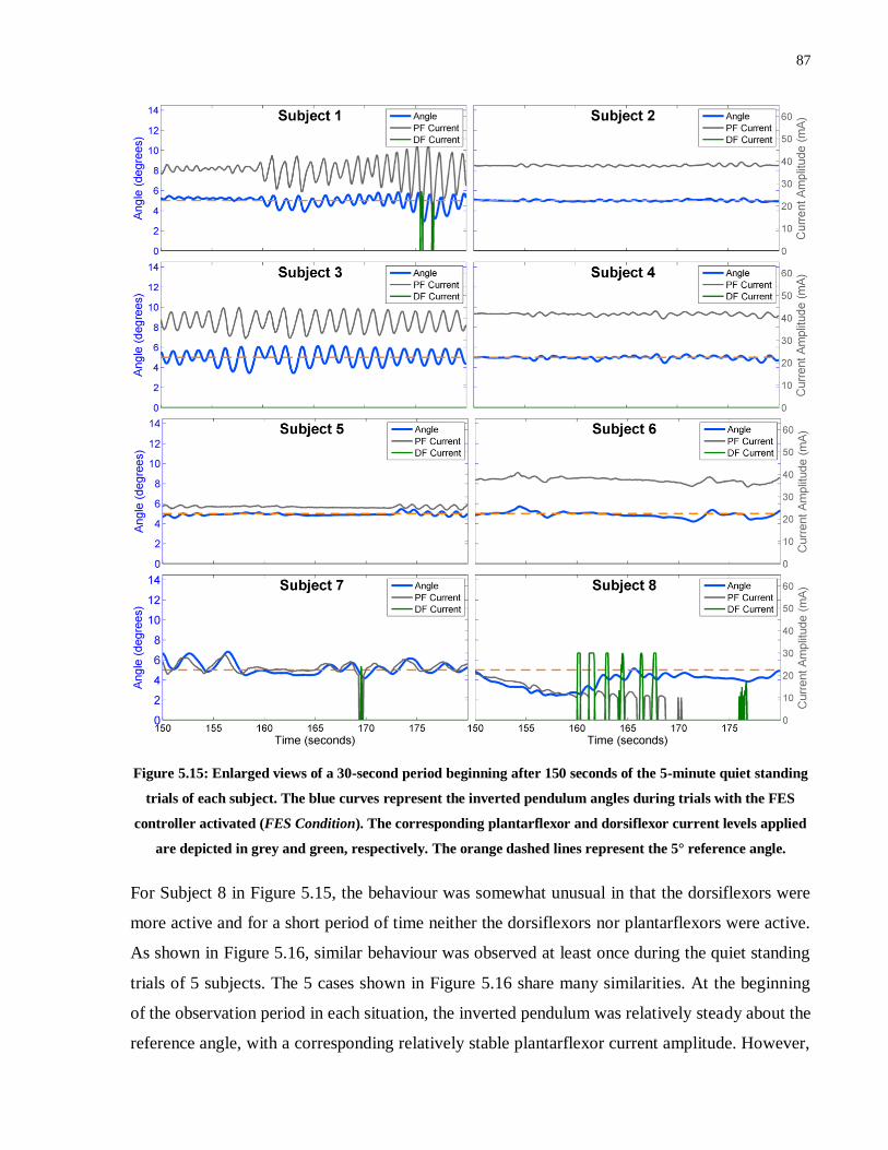
87
Figure 5.15: Enlarged views of a 30-second period beginning after 150 seconds of the 5-minute quiet standing
trials of each subject. The blue curves represent the inverted pendulum angles during trials with the FES
controller activated (FES Condition). The corresponding plantarflexor and dorsiflexor current levels applied
are depicted in grey and green, respectively. The orange dashed lines represent the 5° reference angle.
For Subject 8 in Figure 5.15, the behaviour was somewhat unusual in that the dorsiflexors were
more active and for a short period of time neither the dorsiflexors nor plantarflexors were active.
As shown in Figure 5.16, similar behaviour was observed at least once during the quiet standing
trials of 5 subjects. The 5 cases shown in Figure 5.16 share many similarities. At the beginning
of the observation period in each situation, the inverted pendulum was relatively steady about the
reference angle, with a corresponding relatively stable plantarflexor current amplitude. However,

88
in each case the angle of the inverted pendulum gradually decreased, moving away from the
reference angle and towards the vertical. As such, the plantarflexor current also dropped. In 4 of
the 5 cases, the plantarflexor current actually dropped to 0 mA and in some cases the dorsiflexors
were even activated. However, in all cases the inverted pendulum angle remained relatively
stationary at an angle below the reference angle but still far from the vertical. In the absence of
plantarflexor activation during these periods, the torque due to gravity should theoretically have
caused the inverted pendulum angle to increase rapidly. However, the fact that this did not occur
suggests that voluntary contraction of the muscles was occurring. Given that at the completion of
these trials, all subjects professed that they were not consciously contracting their plantarflexors,
it appears that this behaviour was a product of subconscious stiffening of the muscles, potentially
a by-product of prolonged, continuous FES-induced activation. The extent of this voluntary
contraction would only need to be minor since the inverted pendulum was balancing at angles
quite close to the vertical (~3°-4° in most cases) and the amount of torque required to maintain
the inverted pendulum would have been relatively low. Following a period of varying duration
lasting at least a few seconds, the inverted pendulum would typically drop rapidly until the
plantarflexors were activated once again, which appears to suggest that the relaxation of the
plantarflexors typically occurred suddenly and rapidly. However, due to a prolonged period with
the inverted pendulum above the reference angle, the integral term required time to ‘unwind’ (i.e.
to overcome the large one-sided integral contribution to the required current amplitude), resulting
in the inverted pendulum dropping to an appreciable extent before the plantarflexors became
sufficiently active again. The entire 5-minute trial in Subject 8 provides a good example of this
behaviour, which will henceforth be defined as the ‘integral wind-up’ issue.

89
Figure 5.16: Enlarged views of periods during the 5-minute quiet standing trials in 5 subjects in which the
required FES current applied to the plantarflexors to maintain the inverted pendulum against gravity
decreased over time. The blue curves represent the inverted pendulum angles during trials with the FES
controller activated (FES Condition). The corresponding real-time plantarflexor and dorsiflexor current
levels applied are depicted in grey and green, respectively. The orange dashed lines represent the 5° reference
angle.
Although transient behaviour was analyzed in more detail in subsequent trials (step response,
external perturbations, body weight matching), ability to overcome an offset initial position in
these quiet standing trials was examined. Figure 5.17 highlights the initial 14 seconds of the 5-
minute trials for each subject. From this figure, it is evident that the controller was able to
compensate for initial offset position in all subjects, settling to within close proximity of the
reference angle, without becoming unstable. Moreover, overshoot was limited to a maximum of
3-3.5° in all subjects, and therefore the inverted pendulum did not get too close to the vertical in
any subject, an important consideration for ensuring stability.

90
Figure 5.17: The initial 14 seconds of the 5-minute quiet standing trials for each subject. Inverted pendulum
angles during trials with the FES controller applied (FES Condition in blue) are compared with voluntary
control trials (Voluntary Condition with Eyes Closed in black). The orange dashed lines represent the 5°
reference angle. Rise times and settling times following the offset initial positions are shown in blue for the
FES Condition and black for the Voluntary Condition with Eyes Closed. Rise and settling times that did not
occur within the first 14 seconds of a trial are not shown.
The figure also depicts rise and settling times in the FES Condition and Voluntary Condition with
Eyes Closed for those that occurred within the first 14 seconds. Importantly, in all subjects, a
shorter settling time was observed with the FES Condition, and in 7 of 8 subjects the rise time
was shorter in the FES Condition. As a result, a significantly shorter settling time was calculated

91
in the FES Condition (p < 0.012), whilst there was a trend to significance for rise time (p <
0.069). The median percentage overshoot was larger in the FES Condition, although this is a
natural consequence of faster rise and settling times, and is not considered problematic at the
magnitudes observed. These data are summarized in Table 5.7.
Despite these promising results, sizeable oscillations were present at the beginning of trials in
many subjects, often resulting in larger than desired settling times. However, these oscillations
were not greater than those observed during the Voluntary Condition with Eyes Closed. It was
hypothesized that reducing the delays in the system would help to minimize these oscillations – a
notion that was tested in Experiment 3 (see Section 5.5).
5.4.4 Step Responses
Following the quiet standing trials, step response trials were performed under the FES Condition,
Voluntary Condition Eyes Closed, Standardized FES Condition, and Voluntary Condition Eyes
Open. Figures 5.18 – 5.25 depict the results of these trials in Subjects 1-8, respectively. In each
figure, the black curves represent the inverted pendulum angle during trials, whilst the orange
lines represent the reference angle which switched from 5° to 9° twice during each trial. In
addition, blue plots representing the outputs of simulations performed at the controller gains used
in the FES and Standardized FES Conditions are also shown.
Figure 5.18: Inverted pendulum angles (in black) for Subject 1 during 90-second step response trials in which
the reference angle (in orange) stepped from 5° to 9° and back on 2 occasions. Four experimental paradigms
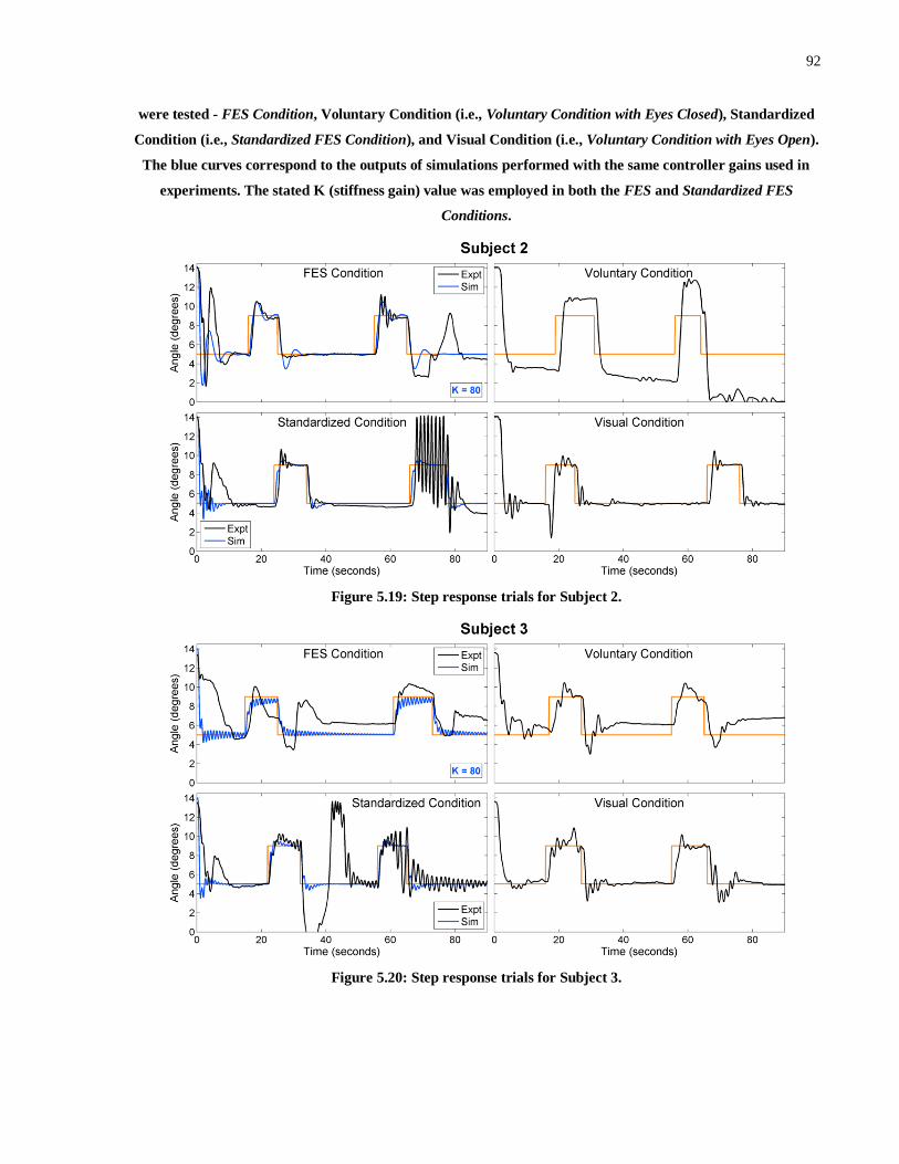
92
were tested - FES Condition, Voluntary Condition (i.e., Voluntary Condition with Eyes Closed), Standardized
Condition (i.e., Standardized FES Condition), and Visual Condition (i.e., Voluntary Condition with Eyes Open).
The blue curves correspond to the outputs of simulations performed with the same controller gains used in
experiments. The stated K (stiffness gain) value was employed in both the FES and Standardized FES
Conditions.
Figure 5.19: Step response trials for Subject 2.
Figure 5.20: Step response trials for Subject 3.

93
Figure 5.21: Step response trials for Subject 4.
Figure 5.22: Step response trials for Subject 5.
Figure 5.23: Step response trials for Subject 6. In this subject, the Standardized FES Condition and Voluntary

94
Condition with Eyes Open were not performed because the subject fainted and was removed from the IPSA
prior to performing these trials.
Figure 5.24: Step response trials for Subject 7.
Figure 5.25: Step response trials for Subject 8. In this subject, the Standardized FES Condition was not
performed and simulations were not tested because the controller had been altered (see Section 5.4.2.1) and
therefore the standardized parameters and simulation parameters were not applicable.
In the FES Condition, the inverted pendulum remained stable throughout the 90-second trials for
Subjects 1-7. Moreover, visual observation suggests that the controller was able to compensate
for step changes to the reference angle reliably, rapidly settling near the new reference angles

95
within a matter of seconds. However, in Subject 8 the ‘integral wind-up’ issue that occurred in
the quiet standing trial caused the inverted pendulum to lose stability, hitting the support surface
at approximately 14° each time the reference angle changed to 9°. As shown in Figure 5.26,
which depicts Subject 8’s step response trial including plantarflexor and dorsiflexor current
levels, this problem occurred as a result of the inverted pendulum angle routinely remaining at
angles less than the reference angle despite very low or no plantarflexor activation, as well as
intermittent dorsiflexor activation. As a result, when the inverted pendulum did drop at the onset
of each step the plantarflexors only became active after the integral term had wound down again.
In the quiet standing trial, the plantarflexors became sufficiently active to prevent the inverted
pendulum reaching the endpoint, but this did not occur here predominantly because the 9°
reference angle meant that the proportional gain contribution was lower.
Figure 5.26: Step response trial in Subject 8 under the FES Condition. The real-time inverted pendulum angle
(blue) is shown, as well as the plantarflexor (grey) and dorsiflexor (green) currents.
In contrast to the results in the FES Condition, stability was only maintained throughout the
Standardized FES Condition trials in 2 of 6 subjects, despite the fact that the standardized
parameters chosen (KP = 140, KD = 0.5, KI = 50) were very close to the mean controller gains
employed across subjects. Note that Subject 6 did not perform the Standardized FES Condition
trial since he fainted and was removed from the experiment prior to this trial. Subject 8 also did
not complete the Standardized FES Condition trial, since the controller had been modified in this
subject, thus changing the definitions of the controller gains. These results in the Standardized
FES Condition suggest that this controller (Controller B) would likely not operate effectively if
designed independent of inter-subject variability, at least not in the configuration employed in
Experiment 2.
0
0.2
0.4
0.6
0.8
1
0 10 20 30 40 50 60 70 80 90
2
4
6
8
10
12
14Subject 8
Angle
(degre
es)
Time (seconds)0 10 20 30 40 50 60 70 80 90
0
10
20
30
40
50
60
Curr
ent A
mplitu
de (
mA
)0
0.2
0.4
0.6
0.8
1
0 10 20 30 40 50 60 70 80 90
2
4
6
8
10
12
14Subject 8
Angle
(degre
es)
Time (seconds)
0 10 20 30 40 50 60 70 80 900
10
20
30
40
50
60
Curr
ent A
mplit
ude (
mA
)
Angle
PF Current
DF Current
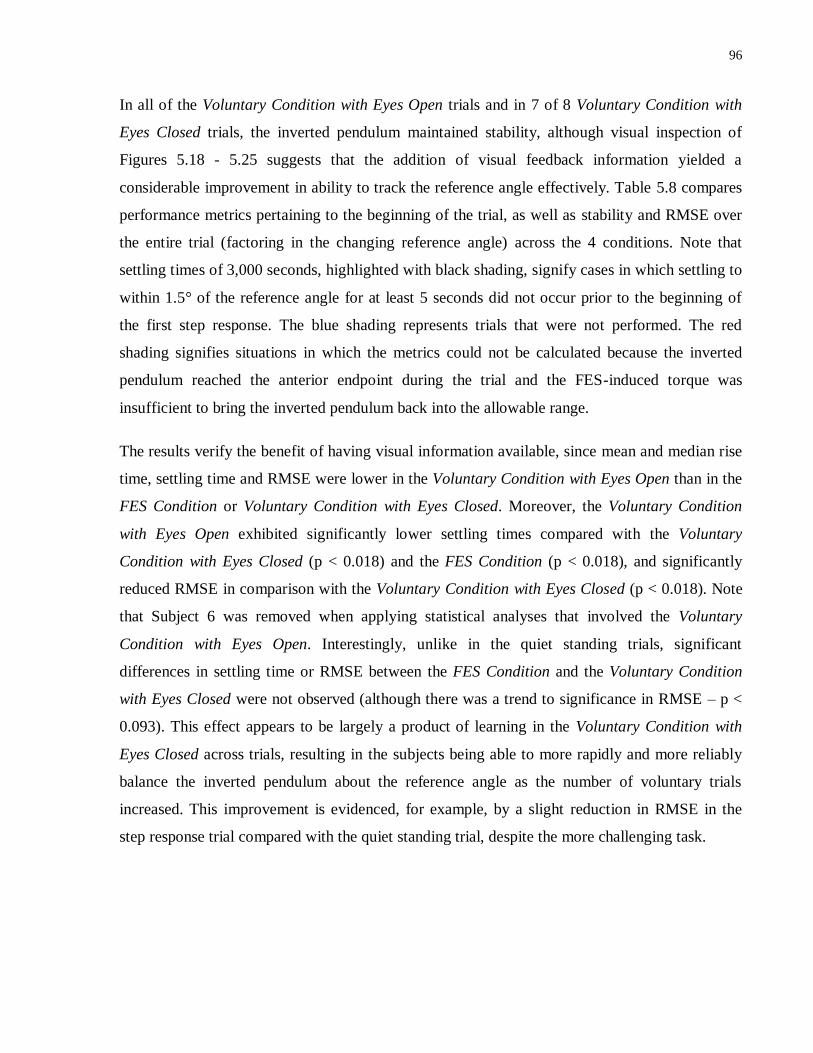
96
In all of the Voluntary Condition with Eyes Open trials and in 7 of 8 Voluntary Condition with
Eyes Closed trials, the inverted pendulum maintained stability, although visual inspection of
Figures 5.18 - 5.25 suggests that the addition of visual feedback information yielded a
considerable improvement in ability to track the reference angle effectively. Table 5.8 compares
performance metrics pertaining to the beginning of the trial, as well as stability and RMSE over
the entire trial (factoring in the changing reference angle) across the 4 conditions. Note that
settling times of 3,000 seconds, highlighted with black shading, signify cases in which settling to
within 1.5° of the reference angle for at least 5 seconds did not occur prior to the beginning of
the first step response. The blue shading represents trials that were not performed. The red
shading signifies situations in which the metrics could not be calculated because the inverted
pendulum reached the anterior endpoint during the trial and the FES-induced torque was
insufficient to bring the inverted pendulum back into the allowable range.
The results verify the benefit of having visual information available, since mean and median rise
time, settling time and RMSE were lower in the Voluntary Condition with Eyes Open than in the
FES Condition or Voluntary Condition with Eyes Closed. Moreover, the Voluntary Condition
with Eyes Open exhibited significantly lower settling times compared with the Voluntary
Condition with Eyes Closed (p < 0.018) and the FES Condition (p < 0.018), and significantly
reduced RMSE in comparison with the Voluntary Condition with Eyes Closed (p < 0.018). Note
that Subject 6 was removed when applying statistical analyses that involved the Voluntary
Condition with Eyes Open. Interestingly, unlike in the quiet standing trials, significant
differences in settling time or RMSE between the FES Condition and the Voluntary Condition
with Eyes Closed were not observed (although there was a trend to significance in RMSE – p <
0.093). This effect appears to be largely a product of learning in the Voluntary Condition with
Eyes Closed across trials, resulting in the subjects being able to more rapidly and more reliably
balance the inverted pendulum about the reference angle as the number of voluntary trials
increased. This improvement is evidenced, for example, by a slight reduction in RMSE in the
step response trial compared with the quiet standing trial, despite the more challenging task.
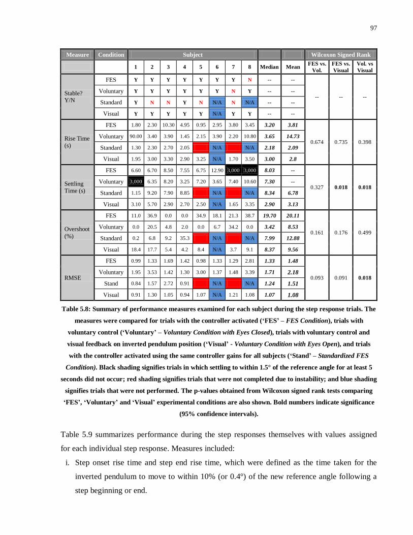
97
Measure Condition Subject Wilcoxon Signed Rank
1 2 3 4 5 6 7 8 Median Mean FES vs.
Vol.
FES vs.
Visual
Vol. vs
Visual
Stable? Y/N
FES Y Y Y Y Y Y Y N -- --
-- -- -- Voluntary Y Y Y Y Y Y N Y -- --
Standard Y N N Y N N/A N N/A -- --
Visual Y Y Y Y Y N/A Y Y -- --
Rise Time (s)
FES 1.80 2.30 10.30 4.95 0.95 2.95 3.80 3.45 3.20 3.81
0.674 0.735 0.398 Voluntary 90.00 3.40 3.90 1.45 2.15 3.90 2.20 10.80 3.65 14.73
Standard 1.30 2.30 2.70 2.05 N/A N/A 2.18 2.09
Visual 1.95 3.00 3.30 2.90 3.25 N/A 1.70 3.50 3.00 2.8
Settling Time (s)
FES 6.60 6.70 8.50 7.55 6.75 12.90 3,000 3,000 8.03 --
0.327 0.018 0.018 Voluntary 3,000 6.35 8.20 3.25 7.20 3.65 7.40 10.60 7.30 --
Standard 1.15 9.20 7.90 8.85 N/A N/A 8.34 6.78
Visual 3.10 5.70 2.90 2.70 2.50 N/A 1.65 3.35 2.90 3.13
Overshoot
(%)
FES 11.0 36.9 0.0 0.0 34.9 18.1 21.3 38.7 19.70 20.11
0.161 0.176 0.499 Voluntary 0.0 20.5 4.8 2.0 0.0 6.7 34.2 0.0 3.42 8.53
Standard 0.2 6.8 9.2 35.3 N/A N/A 7.99 12.88
Visual 18.4 17.7 5.4 4.2 8.4 N/A 3.7 9.1 8.37 9.56
RMSE
FES 0.99 1.33 1.69 1.42 0.98 1.33 1.29 2.81 1.33 1.48
0.093 0.091 0.018 Voluntary 1.95 3.53 1.42 1.30 3.00 1.37 1.48 3.39 1.71 2.18
Stand 0.84 1.57 2.72 0.91 N/A N/A 1.24 1.51
Visual 0.91 1.30 1.05 0.94 1.07 N/A 1.21 1.08 1.07 1.08
Table 5.8: Summary of performance measures examined for each subject during the step response trials. The
measures were compared for trials with the controller activated (‘FES’ – FES Condition), trials with
voluntary control (‘Voluntary’ – Voluntary Condition with Eyes Closed), trials with voluntary control and
visual feedback on inverted pendulum position (‘Visual’ - Voluntary Condition with Eyes Open), and trials
with the controller activated using the same controller gains for all subjects (‘Stand’ – Standardized FES
Condition). Black shading signifies trials in which settling to within 1.5° of the reference angle for at least 5
seconds did not occur; red shading signifies trials that were not completed due to instability; and blue shading
signifies trials that were not performed. The p-values obtained from Wilcoxon signed rank tests comparing
‘FES’, ‘Voluntary’ and ‘Visual’ experimental conditions are also shown. Bold numbers indicate significance
(95% confidence intervals).
Table 5.9 summarizes performance during the step responses themselves with values assigned
for each individual step response. Measures included:
i. Step onset rise time and step end rise time, which were defined as the time taken for the
inverted pendulum to move to within 10% (or 0.4°) of the new reference angle following a
step beginning or end.

98
ii. Step onset settling time and step end settling time, which were defined to have occurred if
the inverted pendulum settled to within 1.5° of the reference angle. For step onset settling
time, settling must have occurred for the remainder of the step and the settling time must
have been at least 2 seconds prior to the end of a step. For step end settling time, settling
must have occurred for at least 5 seconds. Otherwise, values of 3,000 seconds were
assigned.
iii. Step onset overshoot and step end overshoot percentages which were based on the first 8
seconds following the beginning and end of a step, respectively.
iv. RMSE during each step which was defined over the first 8 seconds of each step.
For each of these conditions, black shading signifies that the condition was not met for both
steps, whilst grey shading signifies that the condition was not met in one of the two steps. Table
5.9 also summarizes which subjects and trial conditions resulted in all criteria being met,
including those presented in Table 5.8.
In comparison with the Voluntary Condition with Eyes Closed, the FES Condition performed
more favorably in terms of step onset rise time (p < 0.039) and settling time (p < 0.022), as well
as RMSE during steps (p < 0.010) and the number of subjects meeting all criteria (5/8 vs. 1/8),
verifying the ability of the FES controller to provide benefits over voluntary control in step
response paradigms. The FES Condition also performed admirably in comparison with the
Voluntary Condition with Eyes Open, given that only step end settling time was significantly
higher in the FES Condition (p < 0.011). Moreover, median step onset rise time and RMSE
during steps were comparable in the FES Condition and the Voluntary Condition with Eyes
Open. Step onset (p < 0.019) and step end (p < 0.004) settling times, as well as step end
overshoot were significantly reduced in the Voluntary Condition with Eyes Open compared with
the Voluntary Condition with Eyes Closed. In summary, the FES Condition appeared to perform
better than the Voluntary Condition with Eyes Closed overall, but not quite as well as the
Voluntary Condition with Eyes Open. Detailed comparisons with the Standardized FES
Condition were not performed due to the lower number of successful trials and the fact that
instability was common. Whilst median and mean values are presented in Tables 5.8 and 5.9 for
the Standardized FES Condition, these were calculated for the 4 successful trials, and therefore
the values cannot be directly compared with those obtained in the other trial conditions.
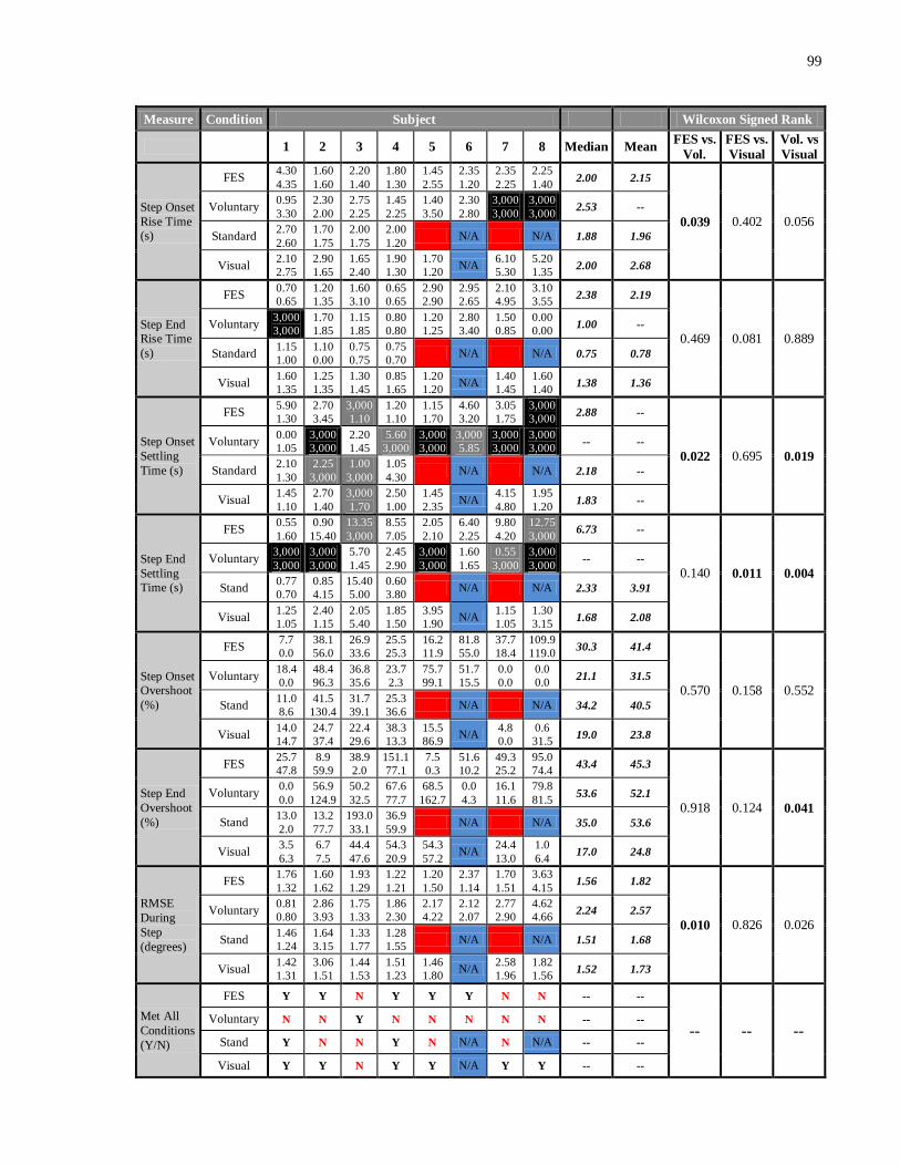
99
Measure Condition Subject Wilcoxon Signed Rank
1 2 3 4 5 6 7 8 Median Mean FES vs.
Vol.
FES vs.
Visual
Vol. vs
Visual
Step Onset
Rise Time
(s)
FES 4.30
4.35
1.60
1.60
2.20
1.40
1.80
1.30
1.45
2.55
2.35
1.20
2.35
2.25
2.25
1.40 2.00 2.15
0.039 0.402 0.056 Voluntary
0.95
3.30
2.30
2.00
2.75
2.25
1.45
2.25
1.40
3.50
2.30
2.80
3,000
3,000
3,000
3,000 2.53 --
Standard 2.70
2.60
1.70
1.75
2.00
1.75
2.00
1.20 N/A N/A 1.88 1.96
Visual 2.10
2.75
2.90
1.65
1.65
2.40
1.90
1.30
1.70
1.20 N/A
6.10
5.30
5.20
1.35 2.00 2.68
Step End
Rise Time
(s)
FES 0.70
0.65
1.20
1.35
1.60
3.10
0.65
0.65
2.90
2.90
2.95
2.65
2.10
4.95
3.10
3.55 2.38 2.19
0.469 0.081 0.889 Voluntary
3,000
3,000
1.70
1.85
1.15
1.85
0.80
0.80
1.20
1.25
2.80
3.40
1.50
0.85
0.00
0.00 1.00 --
Standard 1.15
1.00
1.10
0.00
0.75
0.75
0.75
0.70 N/A N/A 0.75 0.78
Visual 1.60
1.35
1.25
1.35
1.30
1.45
0.85
1.65
1.20
1.20 N/A
1.40
1.45
1.60
1.40 1.38 1.36
Step Onset
Settling
Time (s)
FES 5.90
1.30
2.70
3.45
3,000
1.10
1.20
1.10
1.15
1.70
4.60
3.20
3.05
1.75
3,000
3,000 2.88 --
0.022 0.695 0.019
Voluntary 0.00
1.05
3,000
3,000
2.20
1.45
5.60
3,000
3,000
3,000
3,000
5.85
3,000
3,000
3,000
3,000 -- --
Standard 2.10
1.30
2.25
3,000
1.00
3,000
1.05
4.30 N/A N/A 2.18 --
Visual 1.45
1.10
2.70
1.40
3,000
1.70
2.50
1.00
1.45
2.35 N/A
4.15
4.80
1.95
1.20 1.83 --
Step End
Settling
Time (s)
FES 0.55
1.60
0.90
15.40
13.35
3,000
8.55
7.05
2.05
2.10
6.40
2.25
9.80
4.20
12.75
3,000 6.73 --
0.140 0.011 0.004
Voluntary 3,000
3,000
3,000
3,000
5.70
1.45
2.45
2.90
3,000
3,000
1.60
1.65
0.55
3,000
3,000
3,000 -- --
Stand 0.77
0.70
0.85
4.15
15.40
5.00
0.60
3.80 N/A N/A 2.33 3.91
Visual 1.25
1.05
2.40
1.15
2.05
5.40
1.85
1.50
3.95
1.90 N/A
1.15
1.05
1.30
3.15 1.68 2.08
Step Onset
Overshoot
(%)
FES 7.7
0.0
38.1
56.0
26.9
33.6
25.5
25.3
16.2
11.9
81.8
55.0
37.7
18.4
109.9
119.0 30.3 41.4
0.570 0.158 0.552 Voluntary
18.4
0.0
48.4
96.3
36.8
35.6
23.7
2.3
75.7
99.1
51.7
15.5
0.0
0.0
0.0
0.0 21.1 31.5
Stand 11.0
8.6
41.5
130.4
31.7
39.1
25.3
36.6 N/A N/A 34.2 40.5
Visual 14.0
14.7
24.7
37.4
22.4
29.6
38.3
13.3
15.5
86.9 N/A
4.8
0.0
0.6
31.5 19.0 23.8
Step End
Overshoot
(%)
FES 25.7
47.8
8.9
59.9
38.9
2.0
151.1
77.1
7.5
0.3
51.6
10.2
49.3
25.2
95.0
74.4 43.4 45.3
0.918 0.124 0.041
Voluntary 0.0
0.0
56.9
124.9
50.2
32.5
67.6
77.7
68.5
162.7
0.0
4.3
16.1
11.6
79.8
81.5 53.6 52.1
Stand 13.0
2.0
13.2
77.7
193.0
33.1
36.9
59.9 N/A N/A 35.0 53.6
Visual 3.5
6.3
6.7
7.5
44.4
47.6
54.3
20.9
54.3
57.2 N/A
24.4
13.0
1.0
6.4 17.0 24.8
RMSE
During
Step
(degrees)
FES 1.76
1.32
1.60
1.62
1.93
1.29
1.22
1.21
1.20
1.50
2.37
1.14
1.70
1.51
3.63
4.15 1.56 1.82
0.010 0.826 0.026 Voluntary
0.81
0.80
2.86
3.93
1.75
1.33
1.86
2.30
2.17
4.22
2.12
2.07
2.77
2.90
4.62
4.66 2.24 2.57
Stand 1.46
1.24
1.64
3.15
1.33
1.77
1.28
1.55 N/A N/A 1.51 1.68
Visual 1.42
1.31
3.06
1.51
1.44
1.53
1.51
1.23
1.46
1.80 N/A
2.58
1.96
1.82
1.56 1.52 1.73
Met All
Conditions
(Y/N)
FES Y Y N Y Y Y N N -- --
-- -- -- Voluntary N N Y N N N N N -- --
Stand Y N N Y N N/A N N/A -- --
Visual Y Y N Y Y N/A Y Y -- --
100
Table 5.9: Summary of performance measures over the 2 steps for each subject during the step response
trials. The measures were compared for trials with the controller activated (‘FES’ – FES Condition), trials
with voluntary control (‘Voluntary’ – Voluntary Condition with Eyes Closed), trials with voluntary control and
visual feedback on inverted pendulum position (‘Visual’ - Voluntary Condition with Eyes Open), and trials
with the controller activated using the same controller gains for all subjects (‘Stand’ – Standardized FES
Condition). Black shading signifies trials in which the condition was not met for both step responses within a
trial; grey shading signifies trials in which the condition was not met for one of the two step responses within
a trial; red shading signifies trials that were not completed due to instability; and blue shading signifies trials
that were not performed. The p-values obtained from Wilcoxon signed rank tests comparing FES, Voluntary
and Visual experimental conditions are also shown. Bold numbers indicate significance (95% confidence
intervals).
The step response trials also provided an opportunity to examine the ability of the updated post-
experimentation Simulink model to match experimental behaviour under a number of
circumstances including offset initial positions, quiet standing, and step responses (see Figures
5.18 – 5.25). In these simulations, the voluntary gain (V) was set to 65 Nm/rad for all subjects,
whilst the stiffness gain was varied between subjects to provide maximized matching. The K-
values employed are shown in Figures 5.18 – 5.25. The simulations were able to match the
experimental data to a reasonable extent, particularly in those subjects exhibiting less erratic
behaviour. For example, in Subjects 1, 2 and 5, there was a high level of agreement between
simulated and experimental data in the FES Condition especially, but also in the Standardized
FES Condition. However, it should be noted that the large degree of variability observed
experimentally even within the same subject and trial suggests that accurate modelling of system
behaviour across all subjects and trials is not possible. This variability is exemplified by the fact
that, in many subjects, performance during the first step response varied considerably from
performance in the second step response. For example, in the Standardized FES Condition for
Subjects 2 and 3, the simulations matched the first steps very closely, but in the second steps
very prominent oscillations occurred in the experimental trial. It appears that, particularly in the
presence of large system delays, initially minor deviations from ideal muscle behaviour can
rapidly lead to the development of large oscillations. In Subject 2’s Standardized FES Condition
trial, this minor deviation was likely caused by a small amount of ‘integrator wind-up’ resulting
in the inverted pendulum being maintained slightly below the reference angle prior to the second
step. In Subject 3’s Standardized FES Condition trial, small oscillations prior to the second step
are exacerbated by the step and lead to larger oscillations. The development of large oscillations
101
could then potentially cause instability (as in Subject 5’s Standardized FES Condition).
Despite a lower degree of matching in some of the subjects exhibiting more complex and erratic
experimental behaviour, certain aspects of the simulations’ performance were promising across
almost all subjects. For example, whilst the magnitude of oscillations proved difficult to predict,
the simulations were typically effective at predicting the presence of oscillations. Thus, the
development of paradigms designed to minimize or eradicate prominent oscillations could
potentially be developed. It is also noteworthy that the oscillations observed in simulations were
typically of a higher frequency than those observed experimentally. A likely explanation for this
discrepancy is that simulations were performed using a differential equation solver with a fixed
step size of 0.01 seconds. In other words, the solver operated at a frequency of 100 Hz whilst the
controller in Experiment 2 only operated at 20 Hz. As a result, the potential existed for higher
frequency fluctuations in simulations, compared to actual experiments. A discrete-time rather
than continuous-time model may have overcome this discrepancy, although the issue was
effectively eradicated in Experiment 3 since the operating frequency of the controller was
increased to 100 Hz.
The timing of changes in inverted pendulum angle following step response tasks was also very
similar between simulations and experiments, even though the magnitude of angle changes
varied somewhat. In particular, there was typically a (sometimes brief) period at the onset and
end of each step, during which the inverted pendulum angle and rotational velocity behaviour
coincided closely. In contrast, behaviour whilst overcoming the offset initial position proved
more difficult to predict. In particular, as in Experiment 1, in most subjects, the simulations
predicted a more rapid rise time than what was actually observed. One likely contributory factor
is fatigue. Since the offset initial position requires higher current amplitudes, the effects of
fatigue were more likely to be observed here than at any other period in a trial. In situations in
which immediate separation occurred between the simulated and actual responses, such as in
Subjects 4 and 7, fatigue is a likely explanation. However, another more prominent effect also
contributed to the discrepancy. Due to the higher current amplitudes compared with the other
periods of a trial, the inverted pendulum moved at a higher velocity and over a larger distance.
This likely lead to the instigation of a more pronounced voluntary contribution than what the
model predicted. As a result, dramatic slowing of the inverted pendulum and oscillations in the
angle were observed prior to the inverted pendulum reaching the reference angle in almost all
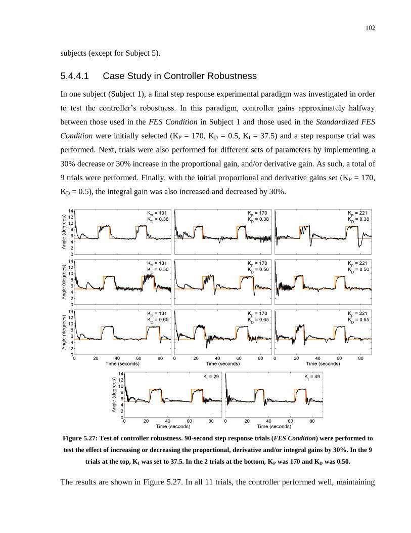
102
subjects (except for Subject 5).
5.4.4.1 Case Study in Controller Robustness
In one subject (Subject 1), a final step response experimental paradigm was investigated in order
to test the controller’s robustness. In this paradigm, controller gains approximately halfway
between those used in the FES Condition in Subject 1 and those used in the Standardized FES
Condition were initially selected (KP = 170, KD = 0.5, KI = 37.5) and a step response trial was
performed. Next, trials were also performed for different sets of parameters by implementing a
30% decrease or 30% increase in the proportional gain, and/or derivative gain. As such, a total of
9 trials were performed. Finally, with the initial proportional and derivative gains set (KP = 170,
KD = 0.5), the integral gain was also increased and decreased by 30%.
Figure 5.27: Test of controller robustness. 90-second step response trials (FES Condition) were performed to
test the effect of increasing or decreasing the proportional, derivative and/or integral gains by 30%. In the 9
trials at the top, KI was set to 37.5. In the 2 trials at the bottom, KP was 170 and KD was 0.50.
The results are shown in Figure 5.27. In all 11 trials, the controller performed well, maintaining

103
the inverted pendulum about the reference angle effectively. Furthermore, there was remarkably
little change in behaviour across trials, and no noticeable drop-off in performance as
proportional, derivative or integral gains changed. As expected, for higher proportional gains the
responses to an offset initial position and to steps was slightly more rapid and more prone to
overshoot, particularly in the trial with the lowest derivative gain. This makes intuitive sense
given that smaller derivative gains would result in less opposition to rapid movement in either
direction. However, the most important point is that the overshoot never became problematic.
These results suggest that the controller is in fact very robust, and that a large range of controller
gains yield similar and acceptable results, at least in this one subject. Nonetheless, it should be
noted that experiments in this subject typically produced better results than the average, and
therefore it cannot be assumed that similar robustness would be achieved in other subjects.
5.4.5 External Perturbations
Following the completion of step response trials, the perturbation bar was applied to the IPSA
and 60-second external perturbation trials were performed under both the FES Condition and the
Voluntary Condition with Eyes Closed (see Figure 5.28). In the figure, arrows (blue for FES
Condition, dark grey for Voluntary Condition with Eyes Closed) represent the timing of posterior
(upwards arrows) and anterior (downwards arrows) perturbations. Note that Subject 6 had been
removed from the experiment prior to these trials after fainting, and Subject 7 did not complete
these trials due to time constraints.
As shown in Figure 5.28, posterior perturbations were overcome without instability occurring in
all subjects with the FES controller activated. Following the posterior perturbation in the
Voluntary Condition with Eyes Closed, instability only occurred (i.e., the inverted pendulum
reached the posterior endpoint) in one subject (Subject 8). In contrast, following anterior
perturbations, instability occurred in 4 subjects in the FES Condition (Subjects 2, 3, 4 and 8) and
4 subjects in the Voluntary Condition with Eyes Closed (Subjects 2, 4, 5 and 8). There are two
likely explanations for the discrepancy between posterior and anterior perturbation response.
First, as discussed in Section 4.2.2, assuming that the pre-perturbation inverted pendulum was at
5° (which is generally a reasonable assumption based on Figure 5.28), the posterior perturbation
would have produced 9.96 Nm of torque, whilst the anterior perturbation would have produced
13.6 Nm of torque. Second, since the dorsiflexors had much lower torque generating ability than
the plantarflexors, it would have become much more difficult to overcome a perturbation in the
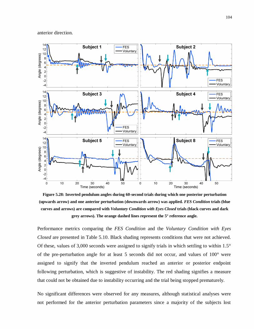
104
anterior direction.
Figure 5.28: Inverted pendulum angles during 60-second trials during which one posterior perturbation
(upwards arrow) and one anterior perturbation (downwards arrow) was applied. FES Condition trials (blue
curves and arrows) are compared with Voluntary Condition with Eyes Closed trials (black curves and dark
grey arrows). The orange dashed lines represent the 5° reference angle.
Performance metrics comparing the FES Condition and the Voluntary Condition with Eyes
Closed are presented in Table 5.10. Black shading represents conditions that were not achieved.
Of these, values of 3,000 seconds were assigned to signify trials in which settling to within 1.5°
of the pre-perturbation angle for at least 5 seconds did not occur, and values of 100° were
assigned to signify that the inverted pendulum reached an anterior or posterior endpoint
following perturbation, which is suggestive of instability. The red shading signifies a measure
that could not be obtained due to instability occurring and the trial being stopped prematurely.
No significant differences were observed for any measures, although statistical analyses were
not performed for the anterior perturbation parameters since a majority of the subjects lost

105
stability. However, as in previous trials, there were notable differences in favour of the FES
Condition for median rise time, settling time and RMSE, as well as stability, peak deviation and
amount of overshoot following posterior perturbations. The fact that fewer subjects completed
these trials likely contributed to the lack of significance.
Measure Condition Subject Wilcoxon
Signed Rank
1 2 3 4 5 8 Median Mean p-value
Stable? (Y/N)
FES Y N N N Y N -- -- --
Voluntary Y N Y N N N -- --
Rise Time (s) FES 2.60 1.90 2.35 1.75 1.10 4.25 2.13 2.33
0.075 Voluntary 30.20 1.95 3.70 1.35 1.80 5.00 2.83 7.33
Settling Time (s)
FES 2.50 7.30 6.65 11.70 2.30 7.10 6.88 6.26 0.345
Voluntary 27.70 19.10 12.40 3.20 0.00 7.35 9.88 11.63
Overshoot (%) FES 0.0 25.9 25.7 35.3 28.2 3.3 25.8 19.7
0.686 Voluntary 0.0 38.4 5.5 9.0 31.6 19.7 14.4 17.4
RMSE (degrees)
FES 0.77 2.40 3.26 1.72 1.52 100 2.06 -- 0.753
Voluntary 1.27 1.78 2.24 2.39 4.58 3.48 2.31 2.62
RMSD (degrees)
FES 0.76 2.39 3.25 1.71 1.38 100 2.05 -- 0.345
Voluntary 1.04 1.30 1.71 1.79 2.08 2.61 1.75 1.76
Peak Posterior Deviation (degrees)
FES 1.87 7.24 3.14 3.34 3.16 9.24 3.25 4.67 0.345
Voluntary 3.50 6.17 2.68 3.59 5.01 100 4.30 --
Settling Time -
Posterior Perturbation (s)
FES 4.40 3.30 6.50 2.30 2.40 10.50 3.85 4.90 0.917
Voluntary 1.20 3,000 2.35 2.05 1.70 3,000 2.20 --
Overshoot - Posterior Pert. (degrees)
FES 2.46 0.00 2.17 1.25 0.00 0.00 0.63 0.98 0.463
Voluntary 0.2 1.59 1.31 2.86 1.37 1.73 1.48 1.51
Peak Anterior Deviation (degrees)
FES 3.72 100 8.14 100 7.18 3,000 8.14 -- --
Voluntary 2.92 100 7.76 100 100 100 -- --
Settling Time –Anterior Perturbation (s)
FES 1.60 16.60 3,000 7.70 13.00 3,000 10.4 -- --
Voluntary 1.45 8.15 3,000 3,000 8.70 5.55 6.85 --
Overshoot – Anterior Pert. (degrees)
FES 0.08 6.87 8.63 3.51 0.58 3.51 3.93 --
Voluntary 1.3 3.51 2.76 0.00 2.72 6.59 2.74 2.81
Table 5.10: Summary of performance measures examined for each subject during the 60-second external
perturbation trials. The measures were compared for trials with the controller activated (‘FES’ – FES
Condition) and trials with voluntary control (‘Voluntary’ - Voluntary Condition with Eyes Closed). Black
shading with values of 3,000 s assigned signify trials in which settling to within 1.5° of the pre-perturbation
angle for at least 5 seconds did not occur; black shading with values of 100° assigned signify the inverted
pendulum reaching an anterior or posterior endpoint following perturbation, which is suggestive of
instability; and red shading signifies a trial that was not completed due to instability. The p-values obtained
106
from Wilcoxon signed rank tests comparing conditions are also shown.
5.4.6 Body Weight Matching
Finally, body weight matching trials were performed in those subjects that were willing to take
part in the experiment (Subjects 1, 3, 4 and 5). Subjects that did not receive up to the maximum
60 mA of current to the plantarflexors were not included in these trials due to potential
difficulties producing sufficient torque to lift the inverted pendulum from the starting point. In
fact, in Subjects 4 and 5, calculations based on the maximum torques produced during
calibration suggested that the FES-induced contraction of the plantarflexor muscles may not
have yielded sufficient torque to lift the inverted pendulum from an angle of 14.5°. As a result,
in these 2 subjects an additional support surface was added such that the inverted pendulum
started from an angle of approximately 9.8°. This support surface was removed after the trials
began, though, to allow the inverted pendulum to sway posteriorly out to 14.5°, if necessary.
The total mass and COM height of the upright bar and additional weights of the inverted
pendulum for each subject are presented in Table 5.11, along with each subject’s actual mass
and approximate COM height, as well as the starting angles of the inverted pendulum. Each
subject’s COM height was approximated as 55% of the subject’s total height114
, with an
additional 0.08 m subtracted to account for the distance from the sole of the foot to the ankle
joint. Ultimately, for each subject the inverted pendulum mass and COM height were always
within 7% of the subject’s actual mass and COM height.
In addition, the moments of inertia of the inverted pendulum also appeared to be in the vicinity
of those that have been estimated for typical human subjects. For example, Maurer and
Peterka115
suggest that an average male subject of weight 76 kg would have a moment of inertia
of 66 kg m2 about the ankle joint. By comparison, in the body weight matching paradigm for
Subject 4, who weighed slightly more than 76 kg, the moment of inertia of the inverted
pendulum was only slightly higher, calculated to be 69.7 kg m2.

107
Participant Subject’s
Mass (kg)
Subject’s
COM (m)
Inverted
Pendulum
Mass (kg)
Inverted
Pendulum
COM (m)
Starting
Angle
(degrees)
Subject 1 63 0.85 61.8 0.82 14.5
Subject 3 73 0.91 70.8 0.85 14.5
Subject 4 77 0.91 77.7 0.88 9.8
Subject 5 83 0.94 81.4 0.89 9.8
Table 5.11: Summary of body weight matching parameters
In Subjects 1 and 5, Voluntary Conditions with Eyes Closed and Eyes Open were tested, as well
as the FES Condition (Figure 5.29), whereas in Subjects 3 and 4 only the Voluntary Condition
with Eyes Open and FES Condition were tested (Figure 5.30). Importantly, in all 4 subjects,
stability was maintained throughout the FES trials, despite the added weight on the inverted
pendulum. In contrast, even with visual feedback about the real-time position of the inverted
pendulum, instability occurred in Subjects 3 and 4 as a result of the inverted pendulum reaching
the posterior endpoint during steps to a 9° reference angle. Moreover, in Subject 5 instability
occurred during transition from an offset initial position in the Voluntary Condition with Eyes
Closed, and stability was almost compromised in the Voluntary Condition with Eyes Open.
By visual inspection, the FES controller was capable of maintaining the inverted pendulum about
the reference angles well in Subjects 1, 4 and 5, despite small oscillations. However, in Subject 3
especially, but also in Subject 4, the ‘integral wind-up’ issue discussed in Section 5.4.3 occurred.

108
Figure 5.29: Inverted pendulum angles (in black) for Subjects 1 and 5 during 90-second step response trials in
the body weight matching paradigm. The FES Condition and Voluntary Conditions with Eyes Closed
(‘Voluntary Condition’) and Eyes Open (‘Visual Condition) were tested. The blue curves correspond to the
results of simulations performed with the same controller gains used in experiments. The K (stiffness gain)
values employed in simulations are listed.

109
Figure 5.30: Inverted pendulum angles (in black) for Subjects 3 and 4 during 90-second step response trials
in the body weight matching paradigm. The FES Condition and Voluntary Condition with Eyes Open (‘Visual
Condition’) were tested. The blue curves correspond to the results of simulations performed with the same
controller gains used in experiments. The K (stiffness gain) values employed in simulations are listed.
Performance measures for the different conditions are summarized in Tables 5.12 and 5.13,
although given the smaller sample size for this set of experiments, no statistical analyses were
performed. Impressively, for all measures across the 2 tables, other than step onset and step end
rise times, performance was better in the FES Condition than the Voluntary Condition with Eyes
Open for at least 2 of the 4 subjects, with mean and median values being at least comparable, and
in some cases much better in the FES Condition. In particular, in all subjects, for step onset and
step end overshoot measures, averaged across the 2 steps for each subject, the FES Condition
produced less overshoot. This is important because overshoot can lead to instability, and it
suggests that the controller was able to account for changes to the reference angle in a controlled
manner. The fact that median step onset and step end settling times were comparable to the
Voluntary Condition with Eyes Open despite less overshoot is also very promising. A lower
mean and median RMSE during steps in the FES Condition is also noteworthy.
Rise times during steps could potentially be considered as less vital than settling times during
steps. Regardless, the reason for the slower rise times with the FES controller can be easily
explained. In the controller design, when the reference angle changes from 5° to 9°, the constant

110
gravity term increases, resulting in an increase in FES amplitude applied to the plantarflexors. At
the lower inverted pendulum total mass used in previous trials, this increase was much smaller
than the decrease in required FES amplitude to the plantarflexors caused by a negative
proportional gain component, resulting in an overall decrease in plantarflexor current and the
inverted pendulum dropping towards the new reference angle. However, at the higher inverted
pendulum mass, the relative contribution of the constant gravity terms increased. As a result, in
some cases (depending on the proportional gain value, total inverted pendulum mass and muscle
dynamics model) there was very little change in FES amplitude applied at the time of the steps.
In fact, in Subject 3, the plantarflexor current increased slightly when the reference angle
changed to 9°, as evidenced by a small anterior movement of the inverted pendulum immediately
following these steps in the simulations for Subject 3 (see Figure 5.30). However, in Subject 3
and other subjects, the integral term increased following the step and caused the current applied
to the plantarflexors to decrease gradually. As a result, the inverted pendulum gradually moved
towards the new reference angle, but the rise time was relatively long. This effect also partially
explains why overshoot was minimized. In the future, slight variations to the control strategy
could overcome this issue. For example, converting the gravity term to the new level could be
performed gradually over a period of a few seconds rather than instantaneously.
Comparisons of performance measures in the previous step response trials to those in the body
weight matching paradigm provide some interesting insights. For most measures, in the FES
Condition, the median values were slightly higher for body weight matching, suggesting a slight
drop in performance, which is to be expected. In fact, there were even slight improvements in
median step onset and step end settling times, as well as step onset and step end overshoot. In
contrast, in the Voluntary Condition with Eyes Open, there were larger drops in performance for
almost all measures. These results suggest that the control strategy may actually be more robust
at the more physiologically relevant body weight matching parameters. However, these results
should be interpreted with some caution given that the subjects in the body weight matching
paradigm were only a subset of the subjects that completed the previous step response trials.

111
Measure Condition Subject
1 3 4 5 Median Mean
Stable? (Y/N)
FES Y Y Y Y -- --
Visual Y N N Y -- --
Voluntary Y N/A N/A N -- --
Rise Time (s)
FES 2.45 4.6 7.65 1.6 3.53 4.08
Visual 2.1 4.75 1.55 12.3 3.43 5.18
Voluntary 3.85 N/A N/A -- --
Settling Time (s)
FES 4.15 3,000 3,000 2.55 -- --
Visual 8.7 10.8 11.25 6.5 9.75 9.31
Voluntary 14.25 N/A N/A -- --
Overshoot (%)
FES 21.0 23.0 0 37.9 22.0 20.5
Visual 25.2 1.13 104 0 13.2 32.6
Voluntary 19.6 N/A N/A -- --
RMSE (degrees)
FES 0.921 2.39 1.81 1.26 1.53 1.60
Visual 1.07 1.44 1.46 1.47 1.45 1.36
Voluntary 1.53 N/A N/A -- --
Table 5.12: Summary of performance measures during the body weight matching step response trials. The
measures were compared for trials with the controller activated (‘FES’ - FES Condition), trials with
voluntary control (‘Voluntary’ - Voluntary Condition with Eyes Closed), and trials with voluntary control and
visual feedback on inverted pendulum position (‘Visual’ - Voluntary Condition with Eyes Open). Black shading
signifies trials in which the condition was not met; red shading signifies trials that were not completed due to
instability; and blue shading signifies trials that were not performed.

112
Measure Condition Subject
1 3 4 5 Median Mean
Step Onset Rise Time (s)
FES 6.65
5.80
1.70
3.20
3.05
7.80
4.60
3.55 4.08 4.54
Visual 1.55
1.25
1.30
2.45
1.15
1.25
1.60
2.05 1.43 1.58
Voluntary 2.00
3,000 N/A N/A -- --
Step End
Rise Time (s)
FES 1.15
3.05
2.85
15.00
2.35
2.35
6.05
6.20 2.95 4.88
Visual 3.00
1.60
6.05
2.00
1.10
1.20
1.95
2.65 1.98 2.44
Voluntary 0.65
0.90 N/A N/A -- --
Step Onset Settling Time (s)
FES 2.00
1.10
3,000
3,000
2.35
3.60
2.25
2.60 2.48 --
Visual 1.30
1.05
3.90
1.65
3,000
1.10
4.35
2.90 2.28 --
Voluntary 3,000
3,000 N/A N/A -- --
Step End Settling Time (s)
FES 4.65
2.10
3,000
3,000
10.90
8.40
1.85
2.45 6.53 --
Visual 1.70
1.35
4.05
1.65
6.50
3,000
14.85
8.85 5.28 --
Voluntary 3.05
2.10 N/A N/A -- --
Step Onset Overshoot (%)
FES 0.0
0.0
68.2
0.0
15.7
0.00
15.0
0.0 0.0 12.4
Visual 17.5
27.1
129.1
36.7
126.9
30.5
104.9
39.1 37.9 64.0
Voluntary 9.3
0.0 N/A N/A -- --
Step End Overshoot
(%)
FES 15.6
0.0
31.8
0.0
75.0
40.2
0.00
0.00 7.8 20.3
Visual 15.9
8.3
2.9
4.7
75.0
61.2
38.3
40.1 27.1 30.8
Voluntary 108.0
38.4 N/A N/A -- --
RMSE during Step (degrees)
FES 1.49
1.21
3.37
1.64
1.01
1.95
1.75
1.97 1.70 1.80
Visual 1.35
1.29
2.00
1.67
2.61
1.41
2.43
2.00 1.84 1.85
Voluntary 2.10
2.38 N/A N/A -- --
Met All Conditions
(Y/N)
FES Y N N Y -- -- Visual Y N N Y -- --
Voluntary N N/A N/A N -- --
Table 5.13: Summary of performance measures over the 2 steps during body weight matching step response
trials. The measures were compared for trials with the controller activated (‘FES’ - FES Condition), trials
with voluntary control (‘Voluntary’ - Voluntary Condition with Eyes Closed), and trials with voluntary control
and visual feedback on inverted pendulum position (‘Visual’ - Voluntary Condition with Eyes Open). Black
shading signifies trials in which the condition was not met for both step responses within a trial; grey shading
signifies trials in which the condition was not met for one of the two step responses within a trial; red shading
signifies trials that were not completed due to instability; and blue shading signifies trials that were not
performed.

113
As in the previous step response trials, the simulations matched the experimental data very well
in some subjects (Subject 1 and 5 especially) and less well in subjects in which more complex,
erratic behaviour was observed. In Subjects 1 and 5, although the magnitude of oscillation was
slightly underestimated by the simulations, the general shape and timing of responses were very
well represented. Even performance during the beginnings of the trials in Subjects 1, 3 and 5
matched well and to a larger extent than in the non-body weight matched trials. This
improvement could be partially explained by the voluntary component becoming proportionally
less influential. In Subject 4, there was a large delay prior to the inverted pendulum beginning to
move, which is likely indicative of fatigue.
In a final, additional trial in Subject 1, a 10-minute body weight matched quiet standing trial was
performed in order to investigate the ability of the controller to operate effectively over
prolonged periods of time and to compensate for FES-induced muscle fatigue. As shown in
Figure 5.31, the inverted pendulum was successfully maintained about the reference angle for the
full 10 minutes. Significantly, there did not appear to be any deterioration in performance over
time, suggesting that the controller was capable of compensating for presumed fatigue
effectively, although the amount of fatigue induced during the trial is difficult to quantify.
Figure 5.31: Inverted pendulum angle (blue) and plantarflexor current amplitude (grey) during a 10-minute
quiet standing trial in Subject 1 with body weight matching (FES Condition). Note that the dorsiflexor
current amplitude was 0 mA throughout the 10-minute trial.
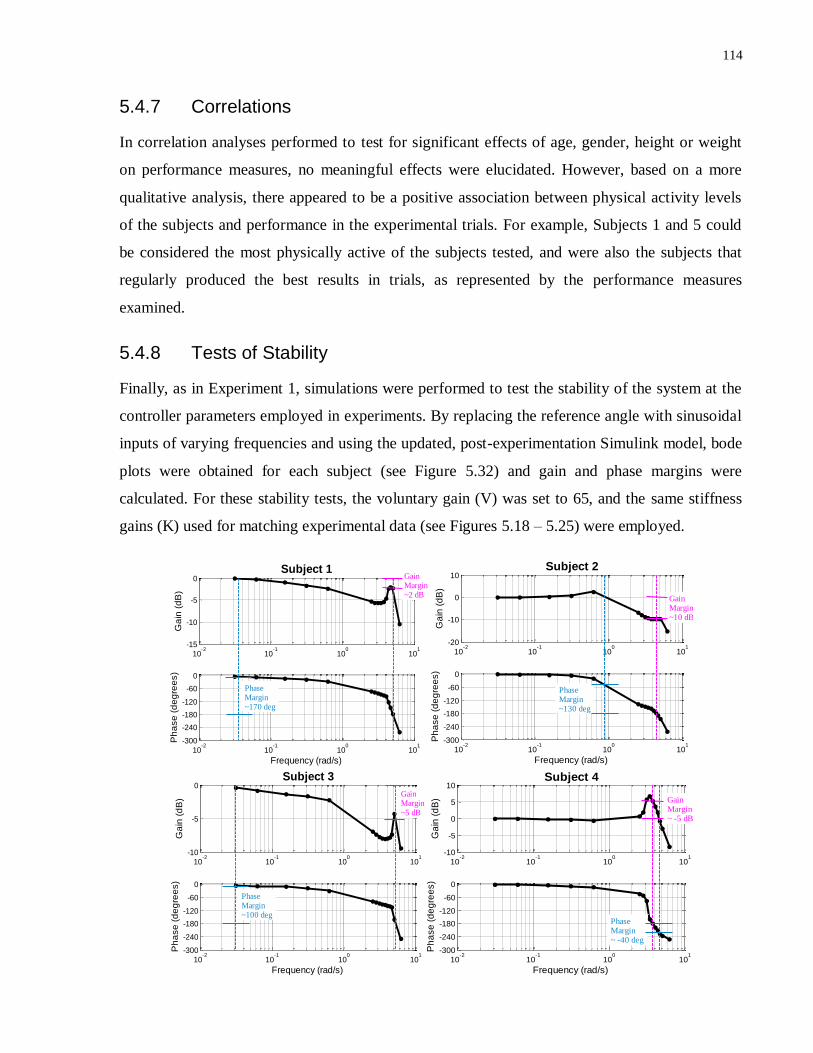
114
5.4.7 Correlations
In correlation analyses performed to test for significant effects of age, gender, height or weight
on performance measures, no meaningful effects were elucidated. However, based on a more
qualitative analysis, there appeared to be a positive association between physical activity levels
of the subjects and performance in the experimental trials. For example, Subjects 1 and 5 could
be considered the most physically active of the subjects tested, and were also the subjects that
regularly produced the best results in trials, as represented by the performance measures
examined.
5.4.8 Tests of Stability
Finally, as in Experiment 1, simulations were performed to test the stability of the system at the
controller parameters employed in experiments. By replacing the reference angle with sinusoidal
inputs of varying frequencies and using the updated, post-experimentation Simulink model, bode
plots were obtained for each subject (see Figure 5.32) and gain and phase margins were
calculated. For these stability tests, the voluntary gain (V) was set to 65, and the same stiffness
gains (K) used for matching experimental data (see Figures 5.18 – 5.25) were employed.
10-2
10-1
100
101
-15
-10
-5
0
Ga
in (
dB
)
Subject 1
10-2
10-1
100
101
-300
-240
-180
-120
-60
0
Frequency (rad/s)
Ph
ase
(d
eg
ree
s)
Gain Margin~2 dB
Phase Margin~170 deg
10-2
10-1
100
101
-20
-10
0
10
Ga
in (
dB
)
Subject 2
10-2
10-1
100
101
-300
-240
-180
-120
-60
0
Frequency (rad/s)
Ph
ase
(d
eg
ree
s)
Phase Margin~130 deg
Gain Margin~10 dB
10-2
10-1
100
101
-10
-5
0
Ga
in (
dB
)
Subject 3
10-2
10-1
100
101
-300
-240
-180
-120
-60
0
Frequency (rad/s)
Ph
ase
(d
eg
ree
s)
Gain Margin~5 dB
Phase Margin~100 deg
10-2
10-1
100
101
-10
-5
0
5
10
Ga
in (
dB
)
Subject 4
10-2
10-1
100
101
-300
-240
-180
-120
-60
0
Frequency (rad/s)
Ph
ase
(d
eg
ree
s)
Gain Margin~ -5 dB
Phase Margin~ -40 deg
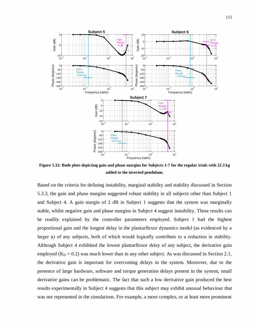
115
Figure 5.32: Bode plots depicting gain and phase margins for Subjects 1-7 for the regular trials with 22.3 kg
added to the inverted pendulum.
Based on the criteria for defining instability, marginal stability and stability discussed in Section
5.3.3, the gain and phase margins suggested robust stability in all subjects other than Subject 1
and Subject 4. A gain margin of 2 dB in Subject 1 suggests that the system was marginally
stable, whilst negative gain and phase margins in Subject 4 suggest instability. These results can
be readily explained by the controller parameters employed. Subject 1 had the highest
proportional gain and the longest delay in the plantarflexor dynamics model (as evidenced by a
larger α) of any subjects, both of which would logically contribute to a reduction in stability.
Although Subject 4 exhibited the lowest plantarflexor delay of any subject, the derivative gain
employed (KD = 0.2) was much lower than in any other subject. As was discussed in Section 2.1,
the derivative gain is important for overcoming delays in the system. Moreover, due to the
presence of large hardware, software and torque generation delays present in the system, small
derivative gains can be problematic. The fact that such a low derivative gain produced the best
results experimentally in Subject 4 suggests that this subject may exhibit unusual behaviour that
was not represented in the simulations. For example, a more complex, or at least more prominent
10-2
10-1
100
101
-10
-5
0
Ga
in (
dB
)
Subject 5
10-2
10-1
100
101
-300
-240
-180
-120
-60
0
Frequency (rad/s)
Ph
ase
(d
eg
ree
s)
Phase Margin~160 deg
Gain Margin~8 dB
10-2
10-1
100
101
-20
-10
0
10
Ga
in (
dB
)
Subject 6
10-2
10-1
100
101
-300
-240
-180
-120
-60
0
Frequency (rad/s)
Ph
ase
(d
eg
ree
s)
Gain Margin~6 dB
Phase Margin~130 deg
10-2
10-1
100
101
-20
-15
-10
-5
0
Ga
in (
dB
)Subject 7
10-2
10-1
100
101
-300
-240
-180
-120
-60
0
Frequency (rad/s)
Ph
ase
(d
eg
ree
s)
Gain Margin~11 dB
Phase Margin~165 deg
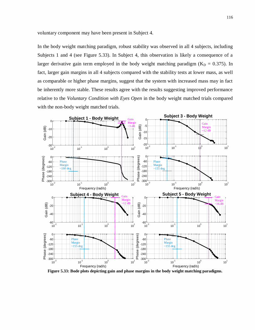
116
voluntary component may have been present in Subject 4.
In the body weight matching paradigm, robust stability was observed in all 4 subjects, including
Subjects 1 and 4 (see Figure 5.33). In Subject 4, this observation is likely a consequence of a
larger derivative gain term employed in the body weight matching paradigm (KD = 0.375). In
fact, larger gain margins in all 4 subjects compared with the stability tests at lower mass, as well
as comparable or higher phase margins, suggest that the system with increased mass may in fact
be inherently more stable. These results agree with the results suggesting improved performance
relative to the Voluntary Condition with Eyes Open in the body weight matched trials compared
with the non-body weight matched trials.
Figure 5.33: Bode plots depicting gain and phase margins in the body weight matching paradigms.
10-2
10-1
100
101
-30
-20
-10
0
Ga
in (
dB
)
Subject 1 - Body Weight
10-2
10-1
100
101
-300
-240
-180
-120
-60
0
Frequency (rad/s)
Ph
ase
(d
eg
ree
s)
Phase Margin~160 deg
Gain Margin~3 dB
10-2
10-1
100
101
-20
-15
-10
-5
0
Ga
in (
dB
)
Subject 3 - Body Weight
10-2
10-1
100
101
-300
-240
-180
-120
-60
0
Frequency (rad/s)
Ph
ase
(d
eg
ree
s)
Phase Margin~155 deg
Gain Margin~12 dB
10-2
10-1
100
101
-60
-40
-20
0
Ga
in (
dB
)
Subject 4 - Body Weight
10-2
10-1
100
101
-300
-240
-180
-120
-60
0
Frequency (rad/s)
Ph
ase
(d
eg
ree
s)
Phase Margin~155 deg
Gain Margin~12 dB
10-2
10-1
100
101
-60
-40
-20
0
Ga
in (
dB
)
Subject 5 - Body Weight
10-2
10-1
100
101
-300
-240
-180
-120
-60
0
Frequency (rad/s)
Ph
ase
(d
eg
ree
s)
Phase Margin~155 deg
Gain Margin~16 dB

117
5.5 Experiment 3 and Comparisons between Experiments
As discussed in Section 4.5.4, a final set of experiments with lower delays in the system was
performed in 3 subjects. Although the small sample sizes in Experiments 1 and 3 made it
difficult to test for significant differences in the outcomes of the 3 systems tested, comparing
outcome measures across experiments is still useful. In particular, comparing the results of the 2
subjects that participated in all 3 experiments was meaningful. For comparing across
experiments, these subjects have been renamed A1i (Subject A in Experiment 1, Subject 1 in
Experiment 2, and Subject i in Experiment 3) and C2ii (Subject C in Experiment 1, Subject 2 in
Experiment 2, and Subject ii in Experiment 3).
5.5.1 Experiment 3 Calibration, Simulations and Fine-Tuning
In Experiment 3, calibration was performed using essentially the same procedure outlined in
Experiment 2, yielding muscle dynamics transfer functions characterized by the K and α values
presented in Table 5.14. Interestingly, the differences between these parameters and those
measured on the same subjects for Experiment 2 were quite pronounced in some cases. For
example, in Subject 1 the plantarflexor α term differed by approximately 40% between
experiments. These differences appear to suggest that muscle behaviour can vary considerably
across days. However, the differences could also potentially point to a limitation of the
calibration method, particularly with regards to modelling torque generation delays.
Subject Plantarflexors Dorsiflexors
K α K α
i 3.02 0.27 0.86 0.17
ii 3.08 0.29 0.98 0.18
iii 5.12 0.33 0.38 0.20
Table 5.14: First order muscle recruitment dynamics model parameters (K and α) for Experiment 3.
Following calibration, simulations were performed using the updated Simulink model presented
in Figure 4.14. The controller gains proposed from these simulations and those ultimately
employed in experiments are presented in Table 5.15 for both the regular experiments and those
with body weight matching. The most dramatic change in both simulation and experimental
parameters was an increase in proportional gains, particularly in Subjects i and ii. Since the
derivative gains are defined in relation to the proportional gains, these increases also signify

118
larger overall derivative components. Given the reduction in delays within the system, it is
logical that stability could be maintained and overshoot could be kept to a minimum, even with
larger controller gains.
Subject Simulations Experiments Simulations
(Body Weight)
Experiments
(Body Weight)
KP
(mA / rad)
KD
(mA / rad s)
KI
(mA s / rad)
RMSE (degs)
KP
(mA / rad)
KD
(mA / rad s)
KI
(mA s / rad)
KP
(mA / rad)
KD
(mA / rad s)
KI
(mA s / rad)
RMSE (degs)
KP
(mA / rad)
KD
(mA / rad s)
KI
(mA s / rad)
i 290 0.4 25 1.25 290 0.4 25 510 0.45 50 1.46 450 0.45 50
ii 290 0.4 25 1.26 260 0.4 25 660 0.4 50 1.16 380 0.55 25
iii 140 0.45 0 1.41 180 0.45 25 -- -- -- -- -- -- --
Table 5.15: Controller gains suggested from simulations performed prior to experiments, and the gains
ultimately employed in experiments for regular and body weight matched trials in Experiment 3. Subject iii
did not perform body weight matched trials.
Since more simplistic simulation models were used to select initial parameters in Experiments 1
and 2, Experiment 3 provided important insight into the potential of the most up-to-date
Simulink models to suggest appropriate parameters for experimentation. Of the 5 cases examined
(including body weight matching for Subjects i and ii), either no changes, or only minor changes
to the proportional gains were required in 4 of the cases. Moreover, in each of these 4 cases,
stability and good performance were achieved with the simulation parameters, but adjustments
were made based on very minor improvements to performance. In contrast, for body weight
matching in Subject ii, adjustments to all 3 parameters were required.
As a consequence of the improved Simulink model, as well as an apparently more robust
controller following the reduction in system delays, considerably fewer fine-tuning trials were
required in Experiment 3 (mean 4.0), compared with Experiment 2 (mean 12.1). Moreover, for
body weight matching only 2 and 3 fine-tuning trials were performed for Subjects i and ii,
respectively. The fact that stability was maintained reliably in Subject iii during fine-tuning trials
was an important finding since the controller was unable to compensate for an offset initial
position in this subject reliably in Experiment 2. Thus, the results suggest a dramatic
improvement caused by the changes implemented for Experiment 3. Moreover, the fact that
reliable stability could be achieved in a subject with unusually high sensitivity to small FES
amplitude fluctuations, verifies the enhanced robustness of the controller.

119
5.5.2 Quiet Standing Trials
Comparisons involving Experiment 1 focused on the quiet standing trials since step responses
were not performed in Experiment 1 and the perturbations were applied using an alternate
technique. For ease of comparison, performance measures for Experiment 1 were recalculated
based on the first 5 minutes of the 10-minute trials.
Figure 5.34 compares 5-minute quiet standing across the 3 experiments for Subject A1i and C2ii.
In Experiment 3, the inverted pendulum was maintained very steadily about the reference angle
with almost no discernible oscillations for the entire 5-minute period in both subjects. In contrast,
small oscillations were evident in the Experiment 1 and 2 trials for both subjects.
The results of the quiet standing trial in Subject iii (i.e. Subject 9 from Experiment 2) are
depicted in Figure 5.35 along with a voluntary control trial. In the FES Condition, stability was
maintained throughout the 5-minute trial, although the ‘integral wind-up’ behaviour observed in
multiple subjects in Experiment 2 was observed.
Figure 5.34: Comparison of 5-minute quiet standing trials (FES Condition) across the 3 experiments in
Subjects A1i and C2ii. For Experiment 1, the first 5 minutes of the 10-minute quiet standing trials are shown.

120
Figure 5.35: 5-minute quiet standing trials for Subject iii in Experiment 3. An FES Condition trial (in blue) is
compared with a Voluntary Condition with Eyes Closed trial (in black).
In Figures 5.36 and 5.37, which depict enlarged views of the first 14 seconds of these trials,
Experiment 3 results are also promising. In particular, in comparison with the Experiment 2
trials, the inverted pendulum appeared to move from an offset initial position in a more
controlled manner with the large oscillations observed in Experiment 2 noticeably reduced. The
controlled nature of the trial onset in Subject iii is also in stark contrast to trials in Experiment 2
(see Figure 5.13). In addition, in Subjects A1i and C2ii, as a result of the larger proportional
gains, in Experiment 3 the inverted pendulum moved more rapidly from the initial angle towards
the reference angle. Interestingly, however, in all 3 subjects in Experiment 3 the inverted
pendulum slowed rapidly at approximately 7°, following which, a more gradual movement
towards 5° was observed. As a result, Experiment 3 actually produced longer rise times
compared with Experiments 1 and 2. However, given that the inverted pendulum moved to
within the vicinity of the reference angle (± 2°-3°) rapidly, this behaviour is not considered
detrimental, and from a clinical standpoint would be considered much more beneficial than large
oscillations. Figure 5.37 also depicts another example of the ‘integral wind-up issue’.
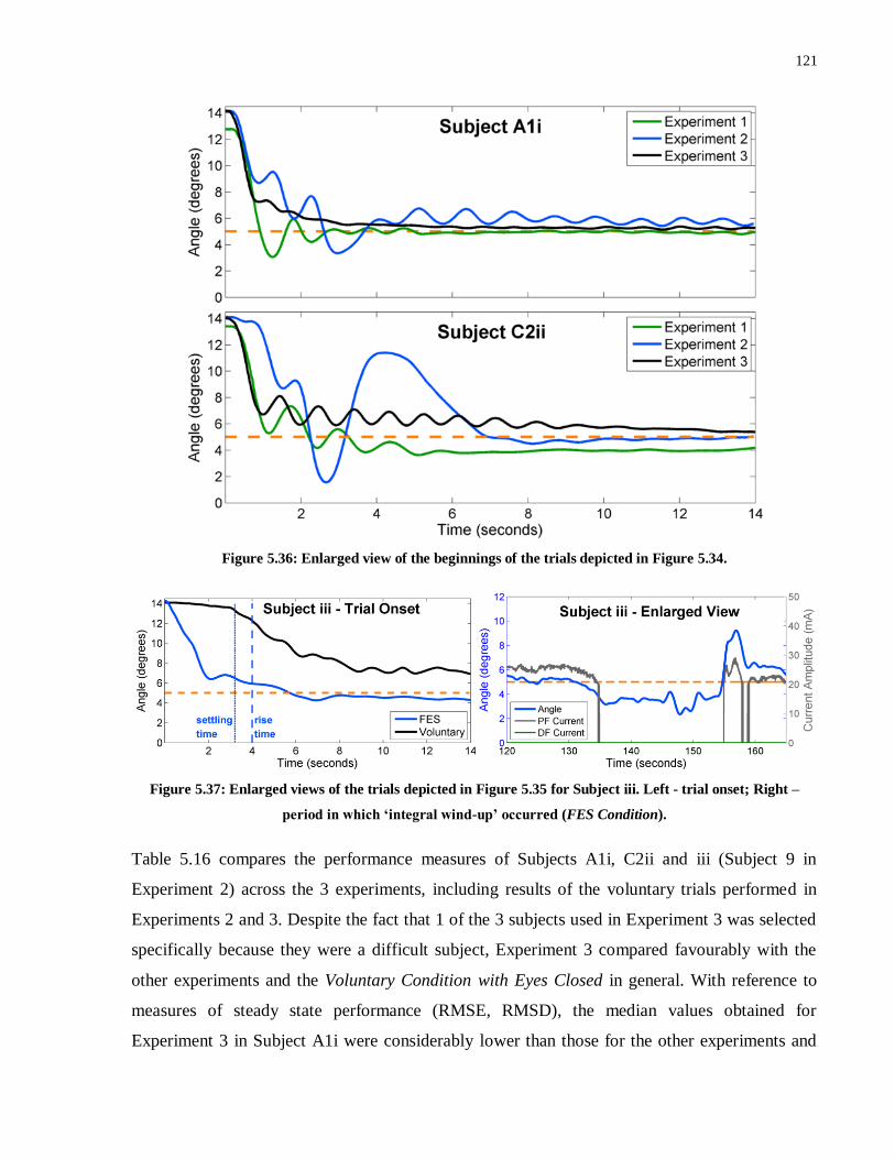
121
Figure 5.36: Enlarged view of the beginnings of the trials depicted in Figure 5.34.
Figure 5.37: Enlarged views of the trials depicted in Figure 5.35 for Subject iii. Left - trial onset; Right –
period in which ‘integral wind-up’ occurred (FES Condition).
Table 5.16 compares the performance measures of Subjects A1i, C2ii and iii (Subject 9 in
Experiment 2) across the 3 experiments, including results of the voluntary trials performed in
Experiments 2 and 3. Despite the fact that 1 of the 3 subjects used in Experiment 3 was selected
specifically because they were a difficult subject, Experiment 3 compared favourably with the
other experiments and the Voluntary Condition with Eyes Closed in general. With reference to
measures of steady state performance (RMSE, RMSD), the median values obtained for
Experiment 3 in Subject A1i were considerably lower than those for the other experiments and

122
the Voluntary Condition with Eyes Closed, whilst in Subject C2ii, improvements were observed
over Experiment 1 and the Voluntary Condition with Eyes Closed and values were comparable
between Experiments 2 and 3. For measures of ability to transition from an offset initial position
(rise time, settling time, overshoot), Experiment 3 also performed much better than the Voluntary
Condition with Eyes Closed and either better than or comparable with Experiment 2 results for
Subjects A1i and C2ii, although rise and settling times were lower in Experiment 1 for both
subjects. However, slightly less restrictive definitions of rise and settling times would have
resulted in Experiment 3 producing the best results. In most measures, Experiment 1 appeared to
perform somewhat better than Experiment 2.
Measure Experiment Subject A1i Subject C2ii Subject iii
Stable?
(Y/N)
1 Y Y N/A
2 Y Y N/A
3 Y Y Y
Voluntary Y Y Y
Rise Time (s)
1 0.86 1.00 N/A
2 2.55 2.20 N/A
3 2.34 2.90 4.00
Voluntary 158.00 7.90 49.68
Settling Time
(s)
1 1.41 1.99 N/A
2 7.65 6.25 N/A
3 1.76 6.27 3.21
Voluntary 142.00 24.10 42.80
Overshoot
(%)
1 25.8 15.6 N/A
2 18.1 37.9 N/A
3 0.0 0.0 8.1
Voluntary 0.0 0.0 0.0
Mean Error
(degrees)
1 0.32 0.048 N/A
2 0.010 0.010 N/A
3 0.024 0.073 0.013
Voluntary 1.52 0.16 0.029
RMSE
(degrees)
1 0.373 0.455 N/A
2 0.37 0.15 N/A
3 0.099 0.18 2.08
Voluntary 1.72 0.39 1.12
RMSD
(degrees)
1 0.185 0.453 N/A
2 0.37 0.15 N/A
3 0.096 0.17 2.08
Voluntary 0.79 0.36 1.12
Table 5.16: Comparison of performance measures obtained in quiet standing trials in Experiments 1-3 with
the FES Condition; as well as the Voluntary Condition with Eyes Closed. Blue shading signifies trials that were
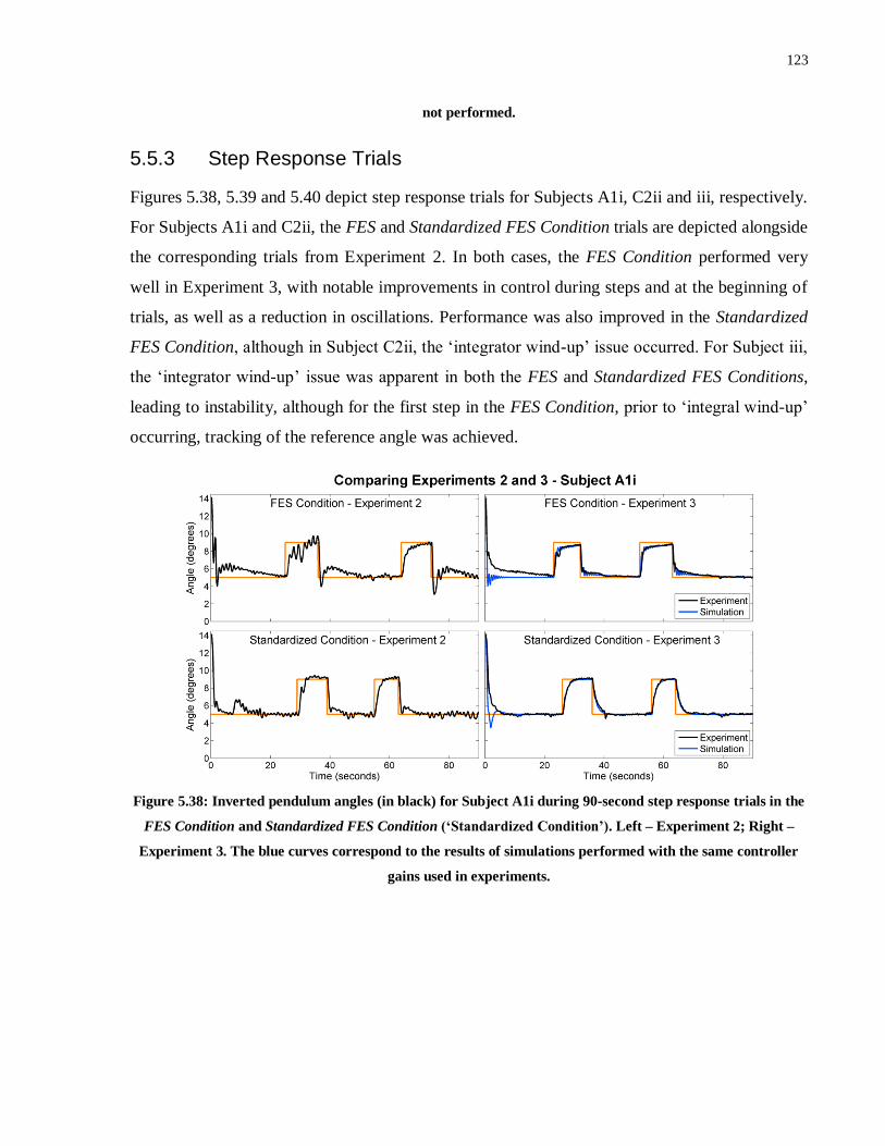
123
not performed.
5.5.3 Step Response Trials
Figures 5.38, 5.39 and 5.40 depict step response trials for Subjects A1i, C2ii and iii, respectively.
For Subjects A1i and C2ii, the FES and Standardized FES Condition trials are depicted alongside
the corresponding trials from Experiment 2. In both cases, the FES Condition performed very
well in Experiment 3, with notable improvements in control during steps and at the beginning of
trials, as well as a reduction in oscillations. Performance was also improved in the Standardized
FES Condition, although in Subject C2ii, the ‘integrator wind-up’ issue occurred. For Subject iii,
the ‘integrator wind-up’ issue was apparent in both the FES and Standardized FES Conditions,
leading to instability, although for the first step in the FES Condition, prior to ‘integral wind-up’
occurring, tracking of the reference angle was achieved.
Figure 5.38: Inverted pendulum angles (in black) for Subject A1i during 90-second step response trials in the
FES Condition and Standardized FES Condition (‘Standardized Condition’). Left – Experiment 2; Right –
Experiment 3. The blue curves correspond to the results of simulations performed with the same controller
gains used in experiments.
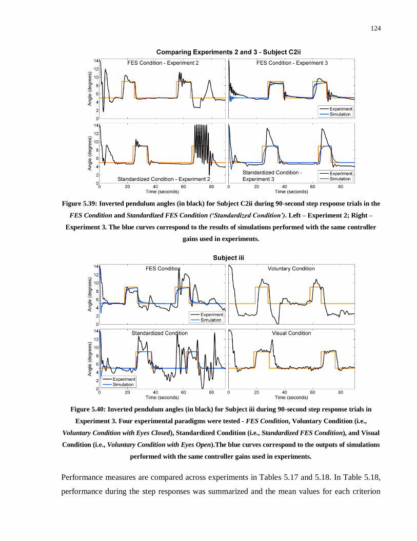
124
Figure 5.39: Inverted pendulum angles (in black) for Subject C2ii during 90-second step response trials in the
FES Condition and Standardized FES Condition (‘Standardized Condition’). Left – Experiment 2; Right –
Experiment 3. The blue curves correspond to the results of simulations performed with the same controller
gains used in experiments.
Figure 5.40: Inverted pendulum angles (in black) for Subject iii during 90-second step response trials in
Experiment 3. Four experimental paradigms were tested - FES Condition, Voluntary Condition (i.e.,
Voluntary Condition with Eyes Closed), Standardized Condition (i.e., Standardized FES Condition), and Visual
Condition (i.e., Voluntary Condition with Eyes Open).The blue curves correspond to the outputs of simulations
performed with the same controller gains used in experiments.
Performance measures are compared across experiments in Tables 5.17 and 5.18. In Table 5.18,
performance during the step responses was summarized and the mean values for each criterion
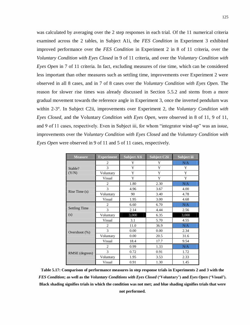
125
was calculated by averaging over the 2 step responses in each trial. Of the 11 numerical criteria
examined across the 2 tables, in Subject A1i, the FES Condition in Experiment 3 exhibited
improved performance over the FES Condition in Experiment 2 in 8 of 11 criteria, over the
Voluntary Condition with Eyes Closed in 9 of 11 criteria, and over the Voluntary Condition with
Eyes Open in 7 of 11 criteria. In fact, excluding measures of rise time, which can be considered
less important than other measures such as settling time, improvements over Experiment 2 were
observed in all 8 cases, and in 7 of 8 cases over the Voluntary Condition with Eyes Open. The
reason for slower rise times was already discussed in Section 5.5.2 and stems from a more
gradual movement towards the reference angle in Experiment 3, once the inverted pendulum was
within 2-3°. In Subject C2ii, improvements over Experiment 2, the Voluntary Condition with
Eyes Closed, and the Voluntary Condition with Eyes Open, were observed in 8 of 11, 9 of 11,
and 9 of 11 cases, respectively. Even in Subject iii, for whom “integrator wind-up” was an issue,
improvements over the Voluntary Condition with Eyes Closed and the Voluntary Condition with
Eyes Open were observed in 9 of 11 and 5 of 11 cases, respectively.
Measure Experiment Subject A1i Subject C2ii Subject iii
Stable? (Y/N)
2 Y Y N/A
3 Y Y Y
Voluntary Y Y Y
Visual Y Y Y
Rise Time (s)
2 1.80 2.30 N/A
3 4.96 3.67 4.00
Voluntary 90 3.40 4.78
Visual 1.95 3.00 4.68
Settling Time
(s)
2 6.60 6.70 N/A
3 2.14 4.44 2.56
Voluntary 3,000 6.35 3,000
Visual 3.1 5.70 4.55
Overshoot (%)
2 11.0 36.9 N/A
3 0.00 0.00 2.34
Voluntary 0.00 20.5 31.6
Visual 18.4 17.7 9.54
RMSE (degrees)
2 0.99 1.33 N/A
3 0.72 0.91 1.72
Voluntary 1.95 3.53 2.33
Visual 0.91 1.30 1.45
Table 5.17: Comparison of performance measures in step response trials in Experiments 2 and 3 with the
FES Condition; as well as the Voluntary Conditions with Eyes Closed (‘Voluntary’) and Eyes Open (‘Visual’).
Black shading signifies trials in which the condition was not met; and blue shading signifies trials that were
not performed.
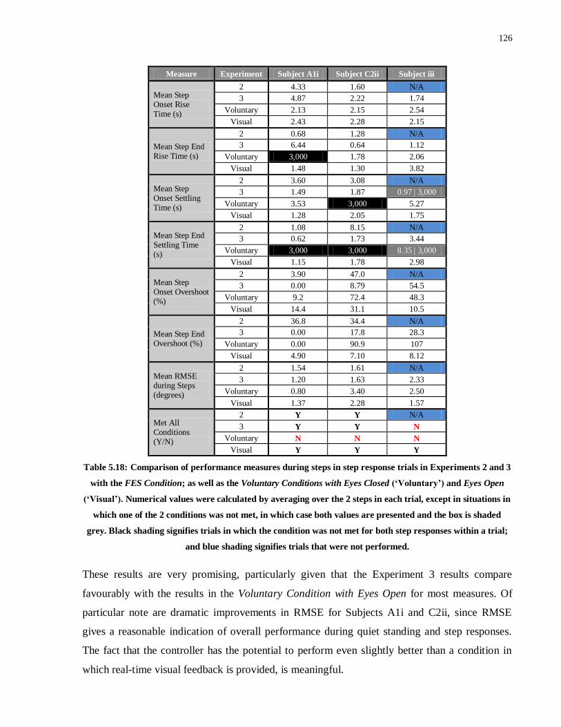
126
Measure Experiment Subject A1i Subject C2ii Subject iii
Mean Step Onset Rise Time (s)
2 4.33 1.60 N/A
3 4.87 2.22 1.74
Voluntary 2.13 2.15 2.54
Visual 2.43 2.28 2.15
Mean Step End Rise Time (s)
2 0.68 1.28 N/A
3 6.44 0.64 1.12
Voluntary 3,000 1.78 2.06
Visual 1.48 1.30 3.82
Mean Step Onset Settling Time (s)
2 3.60 3.08 N/A
3 1.49 1.87 0.97 | 3,000
Voluntary 3.53 3,000 5.27
Visual 1.28 2.05 1.75
Mean Step End Settling Time (s)
2 1.08 8.15 N/A
3 0.62 1.73 3.44
Voluntary 3,000 3,000 8.35 | 3,000
Visual 1.15 1.78 2.98
Mean Step Onset Overshoot (%)
2 3.90 47.0 N/A
3 0.00 8.79 54.5
Voluntary 9.2 72.4 48.3
Visual 14.4 31.1 10.5
Mean Step End Overshoot (%)
2 36.8 34.4 N/A
3 0.00 17.8 28.3
Voluntary 0.00 90.9 107
Visual 4.90 7.10 8.12
Mean RMSE during Steps (degrees)
2 1.54 1.61 N/A
3 1.20 1.63 2.33
Voluntary 0.80 3.40 2.50
Visual 1.37 2.28 1.57
Met All Conditions (Y/N)
2 Y Y N/A
3 Y Y N
Voluntary N N N
Visual Y Y Y
Table 5.18: Comparison of performance measures during steps in step response trials in Experiments 2 and 3
with the FES Condition; as well as the Voluntary Conditions with Eyes Closed (‘Voluntary’) and Eyes Open
(‘Visual’). Numerical values were calculated by averaging over the 2 steps in each trial, except in situations in
which one of the 2 conditions was not met, in which case both values are presented and the box is shaded
grey. Black shading signifies trials in which the condition was not met for both step responses within a trial;
and blue shading signifies trials that were not performed.
These results are very promising, particularly given that the Experiment 3 results compare
favourably with the results in the Voluntary Condition with Eyes Open for most measures. Of
particular note are dramatic improvements in RMSE for Subjects A1i and C2ii, since RMSE
gives a reasonable indication of overall performance during quiet standing and step responses.
The fact that the controller has the potential to perform even slightly better than a condition in
which real-time visual feedback is provided, is meaningful.

127
In Figures 5.38 – 5.40, the blue curves represent the outputs of simulations at the parameters
employed in experiments. Standardized stiffness gain (K = 200) and voluntary gain (V = 65)
values were employed for all 3 subjects. In Subject A1i in particular the simulations matched
almost identically the experimental results, except at the beginning of the trial. This suggests that
the simulations can provide an accurate model of the system, at least in some subjects. The
discrepancy at the beginning of trials, characterized by less overshoot and a more gradual move
towards the reference angle over the final 2-3° in experiments was observed across all 3 subjects.
A possible explanation may be a voluntary contribution which was proportionally greater than
suggested by the simulations and was induced by the high velocity inverted pendulum movement
at the beginning of each trial. The simulations don’t match the experimental results for Subjects
C2ii and iii to the same extent but this discrepancy could be largely explained by the ‘integrator
wind-up’ behaviour observed to a small extent in Subject C2ii and to a much larger extent in
Subject iii. It is also worth noting that although oscillations were less pronounced in the
experimental trials compared with Experiment 2, when they were visible (e.g. the beginning of
Subject C2ii’s trial under the FES Condition, or very minor oscillations observed during much of
Subject A1i’s trials), the frequency of oscillation was more in keeping with the frequency of
oscillations in simulations. This is to be expected given that the Experiment 3 controller
frequency matched the frequency of the differential equation solver in Simulink.
5.5.4 Perturbation Trials
Dramatic improvements between Experiment 2 and Experiment 3 were also observed in the 60-
second perturbation trials. Figure 5.41 compares the results for Subjects A1i and C2ii, whilst
Figure 5.42 depicts the results in the FES Condition and Voluntary Condition with Eyes Closed
for Subject iii. From Figure 5.41, it is evident that less deviation and more rapid settling occurred
following perturbations in either direction in Experiment 3 compared with Experiment 2.
Positive results were also observed for Subject iii although the extent of deviation was increased
compared with the other subjects, most likely due to the presence of ‘integrator wind-up’ once
again. The performance metrics verify these improvements with lower values (indicating
enhanced performance) for Experiment 3 over both Experiment 2 and the Voluntary Condition
with Eyes Closed for 10 of the 11 measures examined in both Subjects A1i and C2ii (see Table
5.19). In Subject iii, improvements or almost identical results were observed over the Voluntary
Condition with Eyes Closed in 10 of 11 measures. These results suggest that the FES Controller
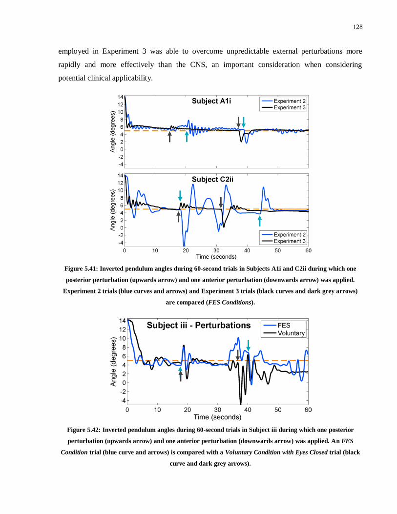
128
employed in Experiment 3 was able to overcome unpredictable external perturbations more
rapidly and more effectively than the CNS, an important consideration when considering
potential clinical applicability.
Figure 5.41: Inverted pendulum angles during 60-second trials in Subjects A1i and C2ii during which one
posterior perturbation (upwards arrow) and one anterior perturbation (downwards arrow) was applied.
Experiment 2 trials (blue curves and arrows) and Experiment 3 trials (black curves and dark grey arrows)
are compared (FES Conditions).
Figure 5.42: Inverted pendulum angles during 60-second trials in Subject iii during which one posterior
perturbation (upwards arrow) and one anterior perturbation (downwards arrow) was applied. An FES
Condition trial (blue curve and arrows) is compared with a Voluntary Condition with Eyes Closed trial (black
curve and dark grey arrows).

129
Measure Experiment Subject A1i Subject C2ii Subject iii
Stable? (Y/N)
2 Y N N/A
3 Y Y Y
Voluntary Y N N
Rise Time (s)
2 2.60 1.90 N/A
3 0.88 2.00 2.49
Voluntary 30.2 1.95 4.87
Settling Time
(s)
2 2.5 7.3 N/A
3 1.58 6.32 2.37
Voluntary 27.7 19.1 8.57
Overshoot (%)
2 0.00 25.9 N/A
3 0.00 0.00 12.1
Voluntary 0.00 38.4 21.9
RMSE
(degrees)
2 0.77 2.40 N/A
3 0.49 0.87 1.81
Voluntary 1.27 1.78 2.63
RMSD
(degrees)
2 0.76 2.39 N/A
3 0.49 0.81 1.79
Voluntary 1.04 1.30 1.76
Peak Posterior Deviation (degrees)
2 1.87 7.24 N/A
3 0.83 1.87 4.12
Voluntary 3.5 6.17 4.05
Settling Time -Posterior Perturbation (s)
2 4.40 3.30 N/A
3 0.00 1.75 3.33
Voluntary 1.2 3,000 2.42
Overshoot - Posterior Perturbation (degrees)
2 2.46 0.00 N/A
3 0.12 0.00 1.02
Voluntary 0.20 1.59 3.57
Peak Anterior Deviation (degrees)
2 3.72 100 N/A
3 2.97 4.85 7.26
Voluntary 2.92 100 100
Settling Time –Anterior Perturbation (s)
2 1.60 16.60 N/A
3 1.30 2.25 3,000
Voluntary 1.45 8.15 3,000
Overshoot – Anterior Perturbation (degrees)
2 0.08 6.87 N/A
3 0.32 1.09 0.50
Voluntary 1.30 3.51 1.78
Table 5.19: Comparison of performance measures obtained in external perturbation trials in Experiments 2
and 3 with the FES Condition; as well as the Voluntary Condition with Eyes Closed. Black shading signifies
trials in which the condition was not met; and blue shading signifies trials that were not performed.
5.5.5 Body Weight Matching
Body weight matching trials were performed in Subjects A1i and C2ii. Subject A1i’s Experiment
2 and Experiment 3 FES Condition trials are depicted along with the Voluntary Condition with
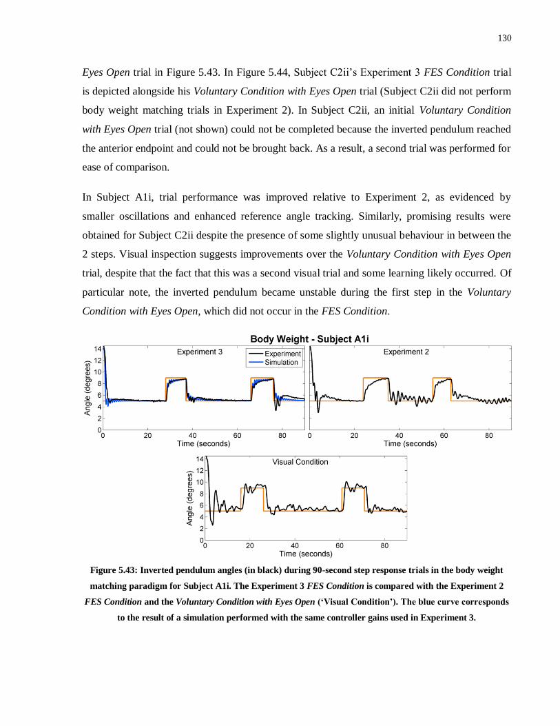
130
Eyes Open trial in Figure 5.43. In Figure 5.44, Subject C2ii’s Experiment 3 FES Condition trial
is depicted alongside his Voluntary Condition with Eyes Open trial (Subject C2ii did not perform
body weight matching trials in Experiment 2). In Subject C2ii, an initial Voluntary Condition
with Eyes Open trial (not shown) could not be completed because the inverted pendulum reached
the anterior endpoint and could not be brought back. As a result, a second trial was performed for
ease of comparison.
In Subject A1i, trial performance was improved relative to Experiment 2, as evidenced by
smaller oscillations and enhanced reference angle tracking. Similarly, promising results were
obtained for Subject C2ii despite the presence of some slightly unusual behaviour in between the
2 steps. Visual inspection suggests improvements over the Voluntary Condition with Eyes Open
trial, despite that the fact that this was a second visual trial and some learning likely occurred. Of
particular note, the inverted pendulum became unstable during the first step in the Voluntary
Condition with Eyes Open, which did not occur in the FES Condition.
Figure 5.43: Inverted pendulum angles (in black) during 90-second step response trials in the body weight
matching paradigm for Subject A1i. The Experiment 3 FES Condition is compared with the Experiment 2
FES Condition and the Voluntary Condition with Eyes Open (‘Visual Condition’). The blue curve corresponds
to the result of a simulation performed with the same controller gains used in Experiment 3.

131
Figure 5.44: Inverted pendulum angles (in black) during 90-second step response trials in the body weight
matching paradigm for Subject C2ii. The Experiment 3 FES Condition is compared with the Voluntary
Condition with Eyes Open (‘Visual Condition’). The blue curve corresponds to the result of a simulation
performed with the same controller gains used in Experiment 3.
The body weight matching performance measures for the 2 subjects are summarized in Table
5.20. In both subjects, almost all measures suggested improved performance in the FES
Condition compared with the Voluntary Condition with Eyes Open. In fact, only step onset rise
time was higher in the FES Condition in Subject C2ii, and only step onset rise time, step onset
settling time and step end overshoot were higher for Subject A1i. Moreover, in Subject A1i,
Experiment 3 results were improved over Experiment 2 results in every measure except step end
overshoot, and even then an overshoot of 23% is not problematic. These results suggest a marked
improvement in control of the inverted pendulum in the FES Condition compared with the
Voluntary Condition with Eyes Open.
Comparison of the Experiment 3 step response results in the FES Condition with and without
body weight matching yield surprisingly little difference in performance metric values. In fact, in
both subjects, rise time, settling time and step onset settling time were actually lower in the body
weight matching paradigm. Furthermore, in Subject C2ii, step onset and step end rise times, step
onset overshoot and RMSE during steps were all also decreased in the body weight matched
scenario. The fact that performance appears not to have been negatively affected by the added
weight on the inverted pendulum, suggests that the controller may actually be better suited to
operating at these more physiologically relevant parameters. This observation can be at least
partially explained by a larger gravity component which helped to minimize the likelihood of
instability occurring due to excessive overshoot and therefore allowed for larger proportional and
derivative gains to be employed. Moreover, the impact of potentially disruptive voluntary control
(as has been observed in the ‘integrator windup’ issue) would have been proportionally reduced.
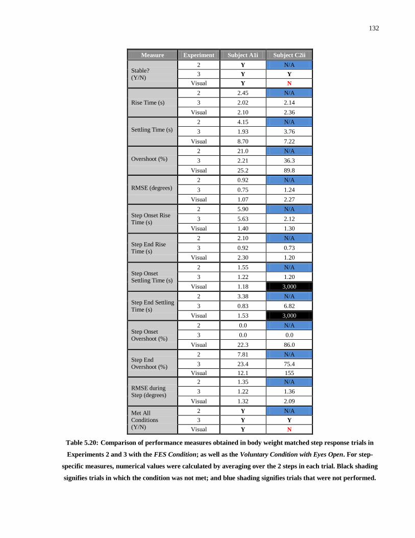
132
Measure Experiment Subject A1i Subject C2ii
Stable? (Y/N)
2 Y N/A
3 Y Y
Visual Y N
Rise Time (s)
2 2.45 N/A
3 2.02 2.14
Visual 2.10 2.36
Settling Time (s)
2 4.15 N/A
3 1.93 3.76
Visual 8.70 7.22
Overshoot (%)
2 21.0 N/A
3 2.21 36.3
Visual 25.2 89.8
RMSE (degrees)
2 0.92 N/A
3 0.75 1.24
Visual 1.07 2.27
Step Onset Rise Time (s)
2 5.90 N/A
3 5.63 2.12
Visual 1.40 1.30
Step End Rise Time (s)
2 2.10 N/A
3 0.92 0.73
Visual 2.30 1.20
Step Onset Settling Time (s)
2 1.55 N/A
3 1.22 1.20
Visual 1.18 3,000
Step End Settling
Time (s)
2 3.38 N/A
3 0.83 6.82
Visual 1.53 3,000
Step Onset Overshoot (%)
2 0.0 N/A
3 0.0 0.0
Visual 22.3 86.0
Step End Overshoot (%)
2 7.81 N/A
3 23.4 75.4
Visual 12.1 155
RMSE during Step (degrees)
2 1.35 N/A
3 1.22 1.36
Visual 1.32 2.09
Met All Conditions (Y/N)
2 Y N/A
3 Y Y
Visual Y N
Table 5.20: Comparison of performance measures obtained in body weight matched step response trials in
Experiments 2 and 3 with the FES Condition; as well as the Voluntary Condition with Eyes Open. For step-
specific measures, numerical values were calculated by averaging over the 2 steps in each trial. Black shading
signifies trials in which the condition was not met; and blue shading signifies trials that were not performed.
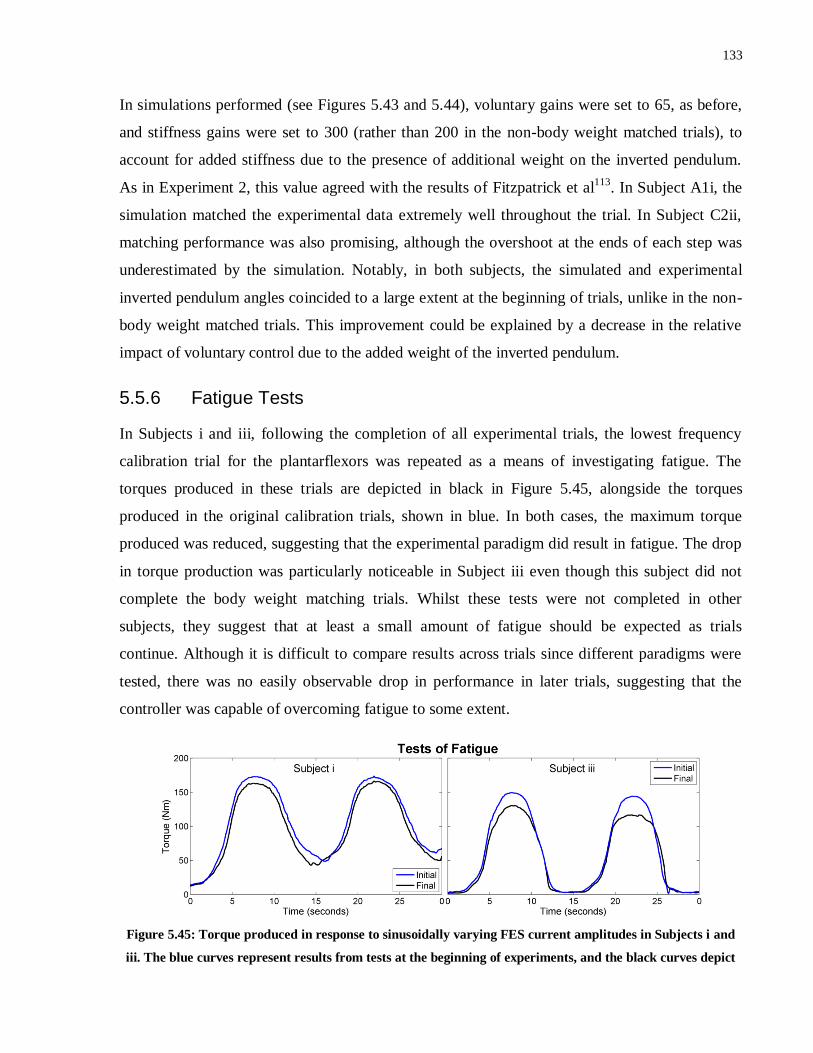
133
In simulations performed (see Figures 5.43 and 5.44), voluntary gains were set to 65, as before,
and stiffness gains were set to 300 (rather than 200 in the non-body weight matched trials), to
account for added stiffness due to the presence of additional weight on the inverted pendulum.
As in Experiment 2, this value agreed with the results of Fitzpatrick et al113
. In Subject A1i, the
simulation matched the experimental data extremely well throughout the trial. In Subject C2ii,
matching performance was also promising, although the overshoot at the ends of each step was
underestimated by the simulation. Notably, in both subjects, the simulated and experimental
inverted pendulum angles coincided to a large extent at the beginning of trials, unlike in the non-
body weight matched trials. This improvement could be explained by a decrease in the relative
impact of voluntary control due to the added weight of the inverted pendulum.
5.5.6 Fatigue Tests
In Subjects i and iii, following the completion of all experimental trials, the lowest frequency
calibration trial for the plantarflexors was repeated as a means of investigating fatigue. The
torques produced in these trials are depicted in black in Figure 5.45, alongside the torques
produced in the original calibration trials, shown in blue. In both cases, the maximum torque
produced was reduced, suggesting that the experimental paradigm did result in fatigue. The drop
in torque production was particularly noticeable in Subject iii even though this subject did not
complete the body weight matching trials. Whilst these tests were not completed in other
subjects, they suggest that at least a small amount of fatigue should be expected as trials
continue. Although it is difficult to compare results across trials since different paradigms were
tested, there was no easily observable drop in performance in later trials, suggesting that the
controller was capable of overcoming fatigue to some extent.
Figure 5.45: Torque produced in response to sinusoidally varying FES current amplitudes in Subjects i and
iii. The blue curves represent results from tests at the beginning of experiments, and the black curves depict
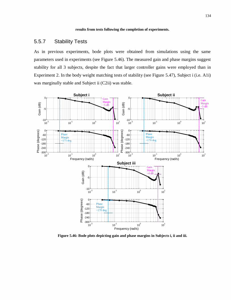
134
results from tests following the completion of experiments.
5.5.7 Stability Tests
As in previous experiments, bode plots were obtained from simulations using the same
parameters used in experiments (see Figure 5.46). The measured gain and phase margins suggest
stability for all 3 subjects, despite the fact that larger controller gains were employed than in
Experiment 2. In the body weight matching tests of stability (see Figure 5.47), Subject i (i.e. A1i)
was marginally stable and Subject ii (C2ii) was stable.
Figure 5.46: Bode plots depicting gain and phase margins in Subjects i, ii and iii.
10-2
10-1
100
101
-10
-5
0
Ga
in (
dB
)
Subject i
10-2
10-1
100
101
-300
-240
-180
-120
-60
0
Frequency (rad/s)
Ph
ase
(d
eg
ree
s)
Phase Margin~175 deg
Gain Margin~5 dB
10-2
10-1
100
101
-10
-5
0
Ga
in (
dB
)
Subject ii
10-2
10-1
100
101
-300
-240
-180
-120
-60
0
Frequency (rad/s)
Ph
ase
(d
eg
ree
s)
Phase Margin~170 deg
Gain Margin~5 dB
10-2
10-1
100
101
-10
-5
0
Ga
in (
dB
)
Subject iii
10-2
10-1
100
101
-300
-240
-180
-120
-60
0
Frequency (rad/s)
Ph
ase
(d
eg
ree
s)
Phase Margin~170 deg
Gain Margin~4 dB
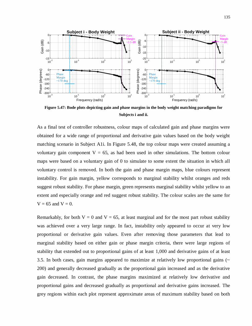
135
Figure 5.47: Bode plots depicting gain and phase margins in the body weight matching paradigms for
Subjects i and ii.
As a final test of controller robustness, colour maps of calculated gain and phase margins were
obtained for a wide range of proportional and derivative gain values based on the body weight
matching scenario in Subject A1i. In Figure 5.48, the top colour maps were created assuming a
voluntary gain component V = 65, as had been used in other simulations. The bottom colour
maps were based on a voluntary gain of 0 to simulate to some extent the situation in which all
voluntary control is removed. In both the gain and phase margin maps, blue colours represent
instability. For gain margin, yellow corresponds to marginal stability whilst oranges and reds
suggest robust stability. For phase margin, green represents marginal stability whilst yellow to an
extent and especially orange and red suggest robust stability. The colour scales are the same for
V = 65 and V = 0.
Remarkably, for both V = 0 and V = 65, at least marginal and for the most part robust stability
was achieved over a very large range. In fact, instability only appeared to occur at very low
proportional or derivative gain values. Even after removing those parameters that lead to
marginal stability based on either gain or phase margin criteria, there were large regions of
stability that extended out to proportional gains of at least 1,000 and derivative gains of at least
3.5. In both cases, gain margins appeared to maximize at relatively low proportional gains (~
200) and generally decreased gradually as the proportional gain increased and as the derivative
gain decreased. In contrast, the phase margins maximized at relatively low derivative and
proportional gains and decreased gradually as proportional and derivative gains increased. The
grey regions within each plot represent approximate areas of maximum stability based on both
10-2
10-1
100
101
-15
-10
-5
0
Ga
in (
dB
)
Subject i - Body Weight
10-2
10-1
100
101
-300
-240
-180
-120
-60
0
Frequency (rad/s)
Ph
ase
(d
eg
ree
s)
Phase Margin~170 deg
Gain Margin~2.5 dB
10-2
10-1
100
101
-20
-15
-10
-5
0
Ga
in (
dB
)
Subject ii - Body Weight
10-2
10-1
100
101
-300
-240
-180
-120
-60
0
Frequency (rad/s)
Ph
ase
(d
eg
ree
s)
Phase Margin~170 deg
Gain Margin~5 dB
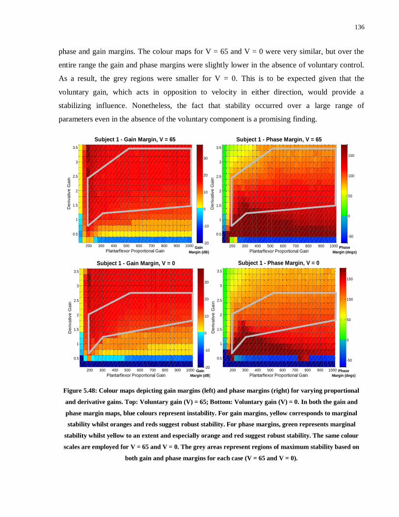
136
phase and gain margins. The colour maps for V = 65 and V = 0 were very similar, but over the
entire range the gain and phase margins were slightly lower in the absence of voluntary control.
As a result, the grey regions were smaller for V = 0. This is to be expected given that the
voluntary gain, which acts in opposition to velocity in either direction, would provide a
stabilizing influence. Nonetheless, the fact that stability occurred over a large range of
parameters even in the absence of the voluntary component is a promising finding.
Figure 5.48: Colour maps depicting gain margins (left) and phase margins (right) for varying proportional
and derivative gains. Top: Voluntary gain (V) = 65; Bottom: Voluntary gain (V) = 0. In both the gain and
phase margin maps, blue colours represent instability. For gain margins, yellow corresponds to marginal
stability whilst oranges and reds suggest robust stability. For phase margins, green represents marginal
stability whilst yellow to an extent and especially orange and red suggest robust stability. The same colour
scales are employed for V = 65 and V = 0. The grey areas represent regions of maximum stability based on
both gain and phase margins for each case (V = 65 and V = 0).
200 300 400 500 600 700 800 900 1000
0.5
1
1.5
2
2.5
3
3.5
Plantarflexor Proportional Gain
Subject 1 - Gain Margin, V = 65
De
riva
tive
Ga
in
-20
-10
0
10
20
30
Gain
Margin (dB)
200 300 400 500 600 700 800 900 1000
0.5
1
1.5
2
2.5
3
3.5
Plantarflexor Proportional Gain
Subject 1 - Phase Margin, V = 65
De
riva
tive
Ga
in
-50
0
50
100
150
Phase
Margin (degs)
200 300 400 500 600 700 800 900 1000
0.5
1
1.5
2
2.5
3
3.5
Plantarflexor Proportional Gain
Subject 1 - Gain Margin, V = 0
De
riva
tive
Ga
in
-20
-10
0
10
20
30
Gain
Margin (dB)
200 300 400 500 600 700 800 900 1000
0.5
1
1.5
2
2.5
3
3.5
Subject 1 - Phase Margin, V = 0
Plantarflexor Proportional Gain
De
riva
tive
Ga
in
-50
0
50
100
150
Phase
Margin (degs)

137
Chapter 6
Discussion
6 Discussion
6.1 Overview
In this chapter, the results obtained are summarized, interpreted and discussed, particularly in
relation to their potential clinical significance. In Section 6.2, the overall results of the various
trials across the 3 experiments are discussed, and in Section 6.3 the results of the corresponding
simulations are analyzed. Finally, in Section 6.4 the major limitations of the study are presented,
along with lines of recommended future research aimed at overcoming these limitations and
ultimately moving towards potential clinical applications.
6.2 Experimental Results
6.2.1 Voluntary Conditions with Eyes Open/Closed
In general, subjects experienced considerable difficulty in maintaining the inverted pendulum
about the reference angle reliably in the Voluntary Condition with Eyes Closed. This included
difficulty ascertaining and maintaining the 5° reference angle, despite a brief period prior to
voluntary trials beginning in which subjects could practice balancing the inverted pendulum at
the reference angle with visual feedback. In addition, the amount of sway and drift of the
inverted pendulum (as characterized by RMSD values) exceeded that observed during able-
bodied stance. In previous studies23,116
, mean COM RMSD in the A/P direction during able-
bodied quiet stance has been calculated as approximately 0.6 cm, which corresponds to a mean
angular deviation of approximately 0.4°. In comparison, in the quiet standing paradigm
employed in Experiment 2, the mean RMSD in the Voluntary Condition with Eyes Closed was
much higher than this (1.01°) even though the weight of the inverted pendulum was much less
than body weight in this paradigm (see Table 5.7). These results verify that use of the IPSA to
suppress vestibular, visual and some proprioceptive sensory inputs did in fact cause a disruption
to voluntary control. As such, any improved results in the FES Condition over the Voluntary
Condition with Eyes Closed can be considered indicative of the potential of the control strategy
to overcome deficits in voluntary control.
138
Thus, these results verify the potential of the IPSA as a tool to assist in the continued
development of closed-loop FES control strategies (PID or other control strategies) for the ankle
joint. In particular, the ability to parse out functional improvements in stability is meaningful,
since it is difficult to test controller performance in able-bodied subjects under normal
circumstances due to the high level of voluntary control. By facilitating the suppression of
multiple sensory mechanisms vital for maintaining stability during stance, the IPSA can be used
with able-bodied subjects to mimic to some extent the impaired sensory systems observed in
different patient populations. Thus, important insights can be obtained whilst avoiding potential
difficulties related to recruitment, heterogeneity and safety in patient populations.
As expected, with the addition of visual feedback on the real-time angle of the inverted
pendulum, ability to balance the inverted pendulum at the reference angle greatly improved, as
evidenced by significant decreases in offset initial position and step response settling times, as
well as RMSE, compared with the Voluntary Condition with Eyes Closed (see Tables 5.8 and
5.9). Nonetheless, small oscillations of similar magnitude to those observed during regular, eyes
open quiet stance were observed about the reference angle in the non-body weight matched
paradigm. In contrast, in the body-weight matching paradigm, most subjects experienced
considerable difficulty balancing the inverted pendulum even with visual input, as evidenced by
the inverted pendulum reaching an endpoint during Voluntary Condition with Eyes Open trials in
3 of the 5 subjects that completed body weight matching trials (see Figures 5.30 and 5.44). The
increased difficulty of this task compared with normal quiet standing is indicative of the
importance of vestibular and proprioceptive information for stability, particularly when relatively
large movement is required117
. Another explanation is that some of the requirements of the
experimental protocol, such as 4° steps in the reference angle, would not typically occur in quiet
stance and as a result the CNS would not be trained in providing the requisite torque levels. In
addition, whilst control of the inverted pendulum simulates quiet stance to an extent, the
subject’s familiarity with this paradigm is obviously not as high as it is with quiet standing.
Moreover, where large movements are required during quiet stance (e.g. following a
perturbation) movement at the knee and hip joints, or stepping, contribute to maintenance of
stability, all of which cannot occur in the IPSA.
139
6.2.2 Trials with the FES Controller
6.2.2.1 Overview
Once appropriate controller parameters were established, the PID plus gravity compensation
control strategy was able to maintain the IPSA’s stability reliably and reproducibly during
prolonged quiet stance and in the presence of offset initial positions, step responses and external
perturbations for the majority of subjects across all 3 experimental paradigms. Despite the
differences in control strategies and system delays across the 3 experiments, considerable
benefits over voluntary control in terms of minimizing steady state error, responding to an offset
initial position and overcoming perturbations, were consistently observed. This capability of
overcoming deficits in voluntary control could potentially be applied to the problem of
facilitating or improving stance in patient populations such as individuals who have suffered a
stroke or incomplete SCI, or aging individuals.
Another promising aspect observed across all 3 experiments was that the control strategy yielded
a muscle activation pattern that matched to some extent that observed during quiet able-bodied
stance. In particular, the ankle muscle activity was dominated by activation of the plantarflexors,
with only intermittent dorsiflexor activation (see Figures 5.5 and 5.15). This pattern is observed
during quiet stance in able-bodied individuals in which the body is generally positioned
approximately 5o in front of vertical, residual activity of the plantarflexors stops the body from
falling forward, and the dorsiflexors are only briefly activated to counteract posterior sway28
.
Another notable characteristic of the control strategies, particularly in Experiments 1 and 2, but
also to a smaller extent in Experiment 3, was the presence of periodic, high-frequency and
generally small oscillations, as well as small, lower frequency fluctuations about the reference
angle in some subjects. Although these oscillations and fluctuations don’t share precisely the
same characteristics as postural sway during able-bodied quiet stance, they should not be
considered necessarily problematic. Kiemel et al107
established that the able-bodied control
strategy during quiet stance is based on minimizing muscle activation rather than limiting small
fluctuations of the COM. Thus, as long as these oscillations are around the reference angle and
small in magnitude, such behavior is not considered detrimental to standing ability.
140
6.2.2.2 Experiment 1
Although the results of Experiment 1 were somewhat preliminary both in terms of the sample
size and the number of paradigms examined, the results were promising, and were used to guide
experimental design decisions in the subsequent experiments. In all 3 subjects, the FES controller
was able to maintain the inverted pendulum about the reference angle during quiet standing and
in the presence of external perturbations. Furthermore, although the small sample size precluded
the use of statistical analyses, there did appear to be a noticeable improvement over the voluntary
control trials in terms of steady state and transient performance. In addition, the apparent
robustness of the controller, as evidenced by the ease of establishing appropriate parameters and
the ability for the same set of parameters to provide acceptable results in all 3 subjects, was
particularly promising.
The calibration procedure also appeared to operate effectively, and it provided a reliable method
of converting requested torques to required FES amplitudes. The effectiveness of this conversion
process was verified by the ability of the controller to maintain the inverted pendulum near the
reference angle in Subject A’s 10-minute trial, despite the absence of an integral component.
Moreover, the results verified the appropriateness of employing isometric torque recruitment
curves, and suggested that FES-induced torques produced during trials were similar to those
obtained during isometric calibration. This was not surprising given that the ankle angle did not
fluctuate by more than a few degrees from the nominal angle of 5° during experiments,
indicating that length and velocity components of the muscle contraction dynamic should not
play any significant role36
. The advantages and disadvantages of this calibration method and that
employed in Experiments 2 and 3 are discussed in more detail in Section 6.4.2.
6.2.2.3 Experiment 2
Although the relatively large system delays in Experiment 2 impacted performance, the
outcomes of trials were promising overall. Of particular note, with the exception of anterior
perturbations which proved difficult to overcome, in Subjects 1-7 across all FES Condition trials,
including body weight matching trials, stability was reliably maintained throughout. The fact that
this stability was maintained reliably during multiple challenging paradigms suggests that the
stability of the system was robust, at least in those subjects whose muscles did not exhibit
unusual behaviour. Moreover, across Subjects 1-7, the controller was typically able to maintain

141
the inverted pendulum near the reference angle in spite of offset initial positions, step responses
and perturbations. In addition, significant improvements over the Voluntary Condition with Eyes
Closed in terms of settling time, mean error, RMSE, step onset rise and settling times and RMSE
during steps across different paradigms verified relative overall benefits of the FES controller.
Furthermore, in 18 out of a total of 25 performance measures across all paradigms, the median
values were lower in the FES Condition over the Voluntary Condition with Eyes Closed,
suggesting improved performance in most measures.
The most important and promising results from Experiment 2 were those obtained in the body
weight matching paradigm. Whilst performance in the Voluntary Conditions with Eyes Closed
and Eyes Open deteriorated markedly in comparison with the earlier trials, the drop in
performance in the FES Condition was much less substantial. This finding, coupled with the fact
that stability was maintained more reliably in the FES Condition than in the Voluntary Condition
with Eyes Closed and even the Voluntary Condition with Eyes Open, suggests that the controller
design is particularly appropriate for operating at body weight. Moreover, the results verify the
potential of the controller to provide enhanced stability over a condition in which the only major
sensory modality unavailable was vestibular. This finding is particularly impressive given that
the delays in the system resulted in the controller operating no faster than the CNS.
One of the key advantages suggested for the employment of a PID-type control strategy is the
fact that the CNS appears to employ a similar control strategy. Thus, a benefit of the timing
paradigm employed in Experiment 2 is that the longer system delays totalling approximately 100
ms closely matched the neural transmission delays present in able-bodied stance (see Section
4.3.3). As such, comparison of the outcomes of Voluntary Condition with Eyes Closed/Open
trials with the outcomes of trials with the FES controller can provide some indication of the
similarities and differences between the control strategies. For example, the similarity in delays
helps to explain the similarity in performance between the FES Condition and the Voluntary
Condition with Eyes Closed. In fact, though performance was generally improved in the FES
Condition, much of this improvement can be attributed to the subjects not having an accurate
measure of the reference angle. If offset from the reference angle is discounted, then
performance was actually fairly similar in most subjects, as exemplified by comparable median
RMSD values in the quiet standing trials, as well as similar responses to perturbations.
Moreover, similarities can be observed in many subjects in relation to the magnitude and
142
frequency of oscillations observed, and the speed of response and degree of overshoot following
steps or an offset initial position.
In the body weight matching paradigm, the increased difficulty of the voluntary task appeared to
result in increased benefit of the FES Condition but similarity in performance between the FES
Condition and Voluntary Condition with Eyes Open was observed. In fact, in the Voluntary
Condition with Eyes Open the CNS appeared to operate with a larger proportional gain, resulting
in faster rise times, but less stability. If the proportional gains in the FES controller were
increased it appears likely that similar results could have been obtained.
Therefore, these results appear to be indicative of the CNS employing a PID-type control
strategy in able-bodied stance as previously suggested in the literature29,30,32,33,36
. Furthermore,
they give some indication of the approximate controller gains theoretically employed by the
CNS. Nonetheless, it is important to note that these interpretations are somewhat speculative for
two main reasons. First, balancing of the inverted pendulum is not exactly equivalent to quiet
standing, particularly since various sensory inputs have been disrupted. Second, whilst there
were typically clear similarities between the Voluntary Conditions with Eyes Closed and Eyes
Open and the FES Condition, there were also notable differences in all subjects, which appear
suggestive of the presence of some more complex aspects of the control strategy employed by
the CNS.
Another interesting finding from Experiment 2 was the degree of variability observed across
subjects. In some subjects (most notably Subjects 1 and 5), despite some small oscillations, very
good performance was observed across all paradigms. In contrast, most other subjects’
performances were less consistent overall. In these other subjects, the controller operated
effectively at times, but at other times, unexpected behaviour resulted in less ideal outcomes,
such as the development of large oscillations, or a steady state angle offset from the reference
angle resulting in integrator windup. One likely explanation for the inter-subject variability is
differing levels of overall fitness and in particular varying levels of muscle conditioning between
subjects. Since Subjects 1 and 5 were physically active and therefore likely had better
conditioning in their lower limb muscles, this could have lead to more predictable response to
FES and less likelihood of unexpected fluctuations in torque levels causing fluctuations in the
inverted pendulum angle. Although the effect of muscle conditioning was not quantified, these

143
results suggest that muscle strengthening paradigms could play an important role when
considering clinical viability of the control strategy, particularly given that erratic muscle
response would be a much larger issue in various patient populations7,118
.
In addition, those subjects with better muscle conditioning were likely to have experienced less
fatigue compared with other subjects. Whilst there was no observable drop in performance as the
experiments continued in any subjects, the possibility that fatigue may have negatively impacted
performance in some subjects cannot be discounted. Any negative effects of fatigue could have
been masked by the difficulty comparing performances across different paradigms, as well as a
possible learning aspect to balancing the inverted pendulum in the FES Condition, which could
have partially counteracted any negative effects of fatigue. This learning could have occurred as
the subject became more familiar with the FES and the experimental protocol, resulting in the
CNS providing some subconscious level of control to the ankle muscles to improve stability in
the presence of FES. This learning could potentially explain the strong performance of the
controller in Subject 1 – the only subject to have had extensive experience using the IPSA prior
to performing the experiments. Nonetheless, similar learning presumably occurred (and was
observed in some instances) in the voluntary trials, and so the presence of improved performance
in Subject 1 and other subjects over voluntary control suggests a direct benefit of the controller.
In the future, repeating trials at different stages of an experiment and/or across days could assist
in determining whether and to what extent learning could be influencing controller outcomes.
A final potential explanation for some of the inter-subject variability observed is differing levels
of voluntary activation. In particular, the “integrator windup” issue, which was observed
repeatedly and was the largest issue affecting performance, was characterized by more torque
being produced by the plantarflexors than expected based on the stimulation amplitude. As such,
some degree of voluntary contraction must have been occurring. However, the extent and
frequency of this behaviour varied considerably across subjects and in Subjects 1 and 5 this
behaviour was not observed at all. Though speculative, one possible explanation is that the CNS
subconsciously activates the plantarflexors in order to decrease the necessary stimulation
intensity applied as a protective mechanism to minimize pain and discomfort. It is likely that
since Subjects 1 and 5 would probably have experienced less fatigue than other subjects, they
would also have experienced less discomfort, and as a result the CNS would not have activated
the plantarflexors to a considerable extent. Potential methods of overcoming this “integrator
144
windup” issue are discussed in Section 6.4.7.
Despite considerable inter-subject variability, only the results of Subjects 8 and 9 were somewhat
problematic. In Subject 8, the controller was initially not designed to handle the unusually high
torque produced at low FES amplitudes. However, a small adjustment to the controller to
accommodate FES amplitudes down to 10 mA was effective at overcoming this issue and should
likely be employed in future experiments to ensure that this issue does not recur. This adjustment
could, however, slightly affect how often the dorsiflexors are activated during trials since
plantarflexor activation would take longer to drop to 0 mA. Thus, the possibility of introducing
some degree of coactivation should be investigated. A larger issue, however, is that the
calibration procedure was not equipped to account for this subject’s sensitivity to FES, resulting
in a larger than appropriate constant gravity term. Potential methods of overcoming this issue are
discussed in Section 6.4.2.
Similarly, Subject 9’s sensitivity to small variations in FES amplitude was not ascertained by the
calibration procedure employed. A calibration procedure that incorporated calibration trials
similar to those employed in Experiment 1 would likely have accounted for this behaviour more
effectively and could potentially have decreased the size of fluctuations in FES amplitudes so as
to improve stability. Nonetheless, the greatly improved performance in this subject in
Experiment 3 verified the potential of a faster system response to overcome some of the
deficiencies of the calibration process.
6.2.2.4 Experiment 3
The overall performance improvement from Experiment 2 to Experiment 3 was pronounced.
Moreover, dramatic benefits of the FES Condition were observed over both the Voluntary
Condition with Eyes Closed and Eyes Open. In fact, in the FES Condition in Subjects A1i and
C2ii performance across the various experimental paradigms was generally almost as good as
could reasonably be expected. In Subject iii, the presence of the “integrator windup” issue caused
problems, but the fact that trials were reliably completed and ability to compensate for an offset
initial position was exhibited repeatedly, represent dramatic improvements over Experiment 2.
Taken together, these results suggest that most of the performance issues observed in Experiment
2 (aside from the negative impacts of voluntary control), including large oscillations at the onset
of trials, oscillations during trials and difficulty overcoming external perturbations, could be
145
overcome simply by decreasing the system delays. However, continued testing in more subjects
would provide a clearer indication of the robustness of the controller employed in Experiment 3.
It is difficult to compare these results directly with the results of previous studies examining FES
control of standing, particularly given various discrepancies in the methodologies employed.
Nonetheless, comparison of these results, particularly in Experiment 3, with the results of
Kobravi and Erfanian63
, the most promising paraplegic standing results obtained thus far,
provides insight into potential benefits of the control strategy employed here. First, in Subjects
A1i and C2ii, the absence of fluctuations both in the inverted pendulum angle and in the FES
amplitude applied during quiet standing was noticeable, and in direct contrast to the relatively
large oscillations observed in Kobravi and Erfanian’s study, both in terms of inclination angle
and FES levels applied to both the plantarflexors and dorsiflexors. Obviously in Subject iii the
performance was less strong, but the apparent presence of voluntary control makes comparison
difficult. Second, transition from an offset initial position was much more rapid in our paradigm
(median settling time of 2.8 seconds in the body weight matched condition) compared with their
paradigm despite only a 5° offset (settling times in excess of 10 seconds for all 3 subjects based
on the trials shown). It is also worth noting that, given the obvious importance of minimizing
delays in the system, the higher computational requirements of Kobravi and Erfanian’s
technique63
could signify a limiting factor on performance. It is important to note, however, that
whilst these comparisons help to justify further experimentation with the controller presented
here, additional challenges were present in Kobravi and Erfanian’s study, including the fact that
experiments were performed in complete paraplegic subjects and the fact that inertial sensors
were employed which likely increased measurement noise.
6.2.2.5 Controller Gains
Analysis of the controller gains employed across the 3 experiments also provides interesting
insights. In general, a large amount of inter-subject variability in appropriate controller gains was
observed and the importance of individually tailoring plantarflexor gains to each subject was
verified. In contrast, the decision to fix dorsiflexor gains across subjects, or to match them with
plantarflexor gains, appears justified. However, since the dorsiflexors were only activated
intermittently, it is difficult to analyze their performance fully.
146
Proportional Gains:
In all 3 experiments, there was considerable inter-subject variability in proportional gains
employed. This variability appears to be partially but not completely explained by the varying
levels of torque produced by each subject. Subjects also appeared to differ in their propensity to
maintain stability with large proportional gains, possibly due to differing levels of voluntary
input and/or muscle conditioning. Experiment 1 yielded the highest proportional gains, but
comparison is difficult since these proportional gains mapped the error signal to torque levels as
opposed to FES amplitudes in Experiments 2 and 3. Typically the proportional gains were
substantially higher in Experiment 3 compared with Experiment 2 both in the body weight
matched and regular paradigms, which suggests that less delay in the system allowed for larger
torques and faster movement of the inverted pendulum without potentially destabilizing the
system. The decision to fix proportional dorsiflexor gains in Experiments 2 and 3 appeared to be
justified although a larger gain may have assisted in avoiding the “integrator windup” issue from
occurring.
Derivative Gains:
Considerable inter-subject variability was also observed for the derivative gains. However, in
Experiment 3, the derivative gains were notably lower than in Experiment 2, and also appeared
less variable. Since derivative gains are important for overcoming system delays and predicting
fluctuations in displacement before they occur28
, it makes sense that larger derivative gains
would be beneficial where system delays are highest. However, with lower delay, lower
derivative gains can facilitate more rapid transitions by decreasing the opposition to movement
produced by the derivative term. There also appeared to be a slight increase in derivative gains in
the body weight matching paradigm, particularly in Experiment 3. This could be accounted for
by a decrease in the relative impact of any voluntary control, and also by a need to limit velocity
in the more challenging paradigm.
Integral Gains:
The integral components provided something of a quandary, resulting in large inter-subject
variability in integral gains ultimately employed. On the one hand, the integral terms were vital
for ensuring that the inverted pendulum converged to the reference angle, particularly in the face
of non-ideal muscle behaviour. This non-ideal behaviour encompasses any behaviour not
147
modelled and not suggested by the calibration data. As such, it could include fatigue, voluntary
input, muscle spasms or variability in torque production. Notably, all of these nonidealities
except for voluntary input would be more pronounced in patient populations, and as such larger
integral terms would possibly be required. Previous studies of closed-loop control of stance,
particularly those based on simulations, have used PD rather than PID controllers, avoiding the
use of integral components35,65
, but this is partly because the simulations typically do not account
for nonideal behaviour. However, our results suggest that small integral gains are useful for
reducing steady state error. In our results, there were multiple examples of situations in which the
controller caused the inverted pendulum to shift towards the reference angle but to settle initially
at angles offset by at least 1° - 2° from the reference angle. Then, the integral term would wind
up and gradually bring the inverted pendulum closer to the reference angle. It is also noteworthy
that even in the simulations performed to establish appropriate controller gains, in which
unexpected behaviour was not accounted for, some non-zero integral gains were typically
suggested to minimize RMSE values.
On the other hand, however, the same nonidealities that necessitate the use of an integral
component can also be responsible for the integral term winding up, and potentially causing
instability. This occurrence was observed multiple times, particularly in the “integrator windup”
issue discussed in Section 5.4.3. Furthermore, when considering the clinical objective of
maintaining stable stance, small steady state errors may be considered less critical than
maintaining stability in the presence of internally and externally generated perturbations. Thus,
integral terms should be incorporated with care and the integral gains should not be set
unnecessarily high. However, as discussed in Section 6.4.7, there may be options for minimizing
the “integrator windup” issue in the future that would likely facilitate easier implementation of
integral gains.
6.3 Simulation Results
The performance of simulations helped to determine appropriate controller gains for use in
experiments, provided theoretical justification for much of the behaviour observed
experimentally, and facilitated investigation of the stability of the overall closed-loop system.
Comparison of the different Simulink models utilized has suggested that the final model
employed (see Figure 4.14) in Experiment 3 and post-experimentation in Experiment 2 provided
the most complete and realistic model of actual system behaviour. As such, discussion will focus

148
on this model as opposed to the more simplistic simulations employed in Experiment 1 and
initially in Experiment 2.
In Experiments 2 and 3, the model was able to match the outcomes of experimental trials to a
reasonable extent in the presence of step responses and an offset initial position. In particular, in
certain subjects whose experimental data suggested more ideal muscle behaviour, the simulations
were typically able to predict performance well, including timing considerations, presence and
size of perturbations and degree of overshoot, therefore providing clear validation of the model
employed. In contrast, in certain subjects in whom significant and unexpected voluntary control
appeared to be present even in the absence of rapid movements of the inverted pendulum, the
simulations were less successful. However, this is to be expected given that unusual muscle and
voluntary control behaviour was not modelled. Another promising finding is that the stiffness
gains that provided the best matching in simulations in the body weight matching trials of
Experiments 2 and 3 coincided with stiffness gains suggested in a study using a similar
apparatus113
.
Of particular note was the excellent matching of trial performance in Subject A1i in both the
regular and body weight matching step response trials of Experiment 3. The fact that such a high
degree of matching was obtained even in one subject suggests that in the absence of nonideal
behaviour the model is appropriate, thus providing justification for all of the elements included in
the model. In fact, the simulations appeared to perform better in Experiment 3 in general. This
improvement can be explained partly by the improved performance of the controller in general,
resulting in greater ease of matching. However, the fact that the increased operating frequency of
the controller in Experiment 3 matched the step size of the differential equation solver employed
in simulations likely also improved simulation accuracy.
The simulations performed so as to select controller gains also appeared to operate effectively,
although reliability has not yet been ascertained. In Experiment 2, these simulations were
performed post-experimentation so the validity of the predictions was difficult to determine. In
Experiment 3, the simulations typically suggested gains that resulted in good, near-optimal
performance in fine-tuning trials. However, since Experiment 3 only involved 3 subjects and 5
total simulations, reproducibility cannot be ascertained. Moreover, in one of the 5 simulations
(body weight matching in Subject C2ii), the gains had to be substantially altered. The reason for

149
this discrepancy could have related to the fact that the simulations and trials were performed
from a starting point of approximately 11° rather than 14° and could also have been influenced
by the increased challenge of balancing so much weight (75 kg in this case) and the fact that
simulations were designed to minimize RMSE without necessarily providing more than marginal
stability. In the future, alternate methods of selecting controller gains, potentially based on
stability rather than (or in addition to) minimizing error, could be worth investigating.
Finally, the stability analyses performed provided evidence that the PID controller was able to
consistently stabilize the inherently unstable inverted pendulum, even in body weight matching
paradigms. Moreover, gain and phase margins indicative of robust stability were obtained for a
wide range of proportional and derivative gain values, suggesting that the stability induced by the
control strategy was not overly sensitive to small variations in parameters. It should be noted,
though, that using gain and phase margins to analyze stability in open loop unstable systems
(such as the inverted pendulum) is somewhat more complicated and less reliable than in open
loop stable systems119
. Thus, these results should be interpreted with caution. However, due to
the presence of non-linear components in the model such as saturation blocks and switching
between muscles, it becomes very difficult to analyze stability using alternate methods.
Moreover, the method employed provided a general notion of both the presence and relative
degree of stability.
6.4 Limitations and Future Directions
Listed below are various lines of research that are designed to overcome limitations in the
research presented here, and are considered worthy of pursuit in the near future. In particular, in
working towards the ultimate goal of developing clinically applicable devices or techniques,
much investigation is still required. Notably, none of this research is necessarily contingent on
completion of other research, and as such many of these lines of research could potentially be
performed in parallel.
6.4.1 Performing experiments in more able-bodied subjects
Although the results obtained are promising, the sample sizes employed, particularly in
Experiments 1 and 3, limited the ability to determine the robustness of the control strategy. In
particular, given that substantial inter-subject variability was observed in relation to controller
150
performance, larger sample sizes would be useful. Given that the best results appeared to be
obtained in Experiment 3, testing this paradigm in additional subjects would be particularly
beneficial. In addition, due to differing system delays, the results presented here cannot discount
the possibility that the controller employed in Experiment 1 may offer benefits over the
controller employed in Experiments 2 and 3. Experiments performed without discrepancies in
timing could assist in differentiating the outcomes of each strategy.
6.4.2 Investigating alternative calibration procedures
The calibration procedures employed in all experiments suffered from some limitations. In
Experiment 1, the method did not take into account muscle dynamics, particularly in relation to
torque generation and reduction delays, resulting in overly simplistic simulations. The α-values
obtained in muscle models in Experiment 2 varied from 0.23 to 0.38, and a similar degree of
variability was also observed in a previous study36
, suggesting that real differences exist between
subjects in torque generation delays. This limitation could potentially be overcome by modelling
muscle dynamics based on the rate of increasing and decreasing torque generation at the
beginning and end of stimulation at each FES amplitude step, respectively. A concern, however,
is that the muscle dynamics observed during more gradual variations in FES intensity (e.g., in
response to sinusoidal inputs) may be more representative of behaviour during experimental
trials, in which FES amplitude is continuously varying.
In Experiments 2 and 3, the muscle dynamics was modelled but a first-order relationship
between FES amplitude and torque generation was assumed, which did not fully account for the
complex relationship suggested from experimental observations. In most subjects, this
assumption did not appear detrimental to performance but the results obtained in Subject 8 in
Experiment 2 suggest a potential problem with this assumption, as discussed in Section 6.2.2.3.
In patient populations, less predictable relationships between current amplitude and torque
produced are likely, and therefore this assumption could be even more problematic.
Incorporation of a second calibration technique similar to that employed in Experiment 1 would
be ideal, but this would increase the time required and could induce more fatigue. Thus, methods
of reducing the time and amount of stimulation required should be examined. For example,
pseudorandom binary sequences (PRBS)120
, which encapsulate a range of frequencies, could
potentially be applied to yield a model of muscle dynamics without the need for multiple trials at
different frequencies. Similarly, the Experiment 1 calibration procedure could potentially be

151
shortened by testing fewer FES amplitudes and decreasing the duration of stimulation at each
amplitude.
6.4.3 Performing similar experiments in patient populations
It is important to note that use of the IPSA in able-bodied subjects will not replace
experimentation on patient populations, particularly given that it is impossible to completely
remove voluntary control of muscles in able-bodied individuals, and because the IPSA does not
account for some of the deficiencies observed in neurological patients’ musculoskeletal
dynamics121,122
. As such, one of the most important next steps will be to investigate the ability of
the controller to overcome some of these issues by testing in patient populations, including
complete and incomplete spinal cord injured patients and stroke patients. Use of the IPSA for
this purpose would be beneficial since most of the advantages of using the IPSA (see Section
4.2.1.2) would extend to patient populations, including the ability to isolate the ankle joints,
disrupt voluntary control (in those patients with some voluntary control), vary the weight of the
inverted pendulum, test different standing paradigms, and ensure patient safety.
Our results also suggest that the IPSA, in combination with a PID or other control strategy, could
potentially be used in a clinical capacity for retraining standing ability following incomplete SCI
or stroke. Multiple studies have espoused functional and physiological benefits of therapeutic
strategies utilizing FES for retraining standing and walking ability in these populations123,124
.
Similarly, we believe that training sessions using the IPSA and a closed-loop FES system applied
to the ankle muscles could offer therapeutic benefits by reinforcing requisite muscle activation
patterns and encouraging motor learning, whilst also increasing muscle strength.
6.4.4 Examining methods of better modelling stance in paraplegic or
other patient populations using the IPSA
Methods of using the IPSA in able-bodied subjects to more realistically simulate stance in patient
populations could provide a useful gateway between the current protocol and experiments in
patients. For example, the effect of fatigue could be examined more thoroughly by performing
more experiments at body weight matching paradigms. In addition, unexpected perturbations
could be applied to the reference angle of the inverted pendulum or the level of stimulation
applied in order to mimic other muscle non-idealities often observed in patients with neurologic
152
conditions, including muscle spasms and tremor. Another beneficial line of research would
involve attempts to further minimize voluntary control by disrupting somatosensory inputs from
the feet and ankles. This could potentially be achieved by inducing ischemia to the feet and/or
ankles, applying localized cooling125
or anesthetic agents126
, or applying mechanical vibrations to
the Achilles tendons127,128
.
6.4.5 Testing controller performance in the presence of substantial
measurement noise
An important consideration when investigating clinical viability of a standing neuroprosthesis is
transferability of the system to a portable device. This is of particular concern in our study since
one of the major arguments against the use of a PID control strategy for facilitating stance is that
the derivative terms cause amplification of high frequency measurement noise62
. In a portable
system, the use of inertial sensors on the human body would likely result in more substantial
noise than that observed using the IPSA with a laser displacement sensor. The potential of this
control strategy to handle more noise could be tested in actual standing trials (i.e. without the
IPSA) using inertial sensors, but issues would arise related to high levels of voluntary control in
able-bodied subjects, as well as safety and recruitment issues in patient populations.
Alternatively, modelling measurement noise in the IPSA by applying small fluctuations to the
reference angle would be useful and simpler to implement. Then, the ability of the controller to
overcome this noise would provide a preliminary indicator of the potential transferability of the
controller to portable systems.
6.4.6 Expanding the Simulink models to incorporate patient populations
Prior to beginning experiments in patient populations, it would be useful to modify the
simulations employed in this study in order to account for some of the differences between
patients with neurological disorders and able-bodied subjects. This notion was investigated
briefly by performing stability analyses with the voluntary control component of simulations
removed. However, other aspects, such as models of musculoskeletal dynamics which
incorporate fatigue, diminished torque generating ability and spasticity, would also be useful. In
previous research performed by our lab, Lynch et al121,129
developed a Simulink block that
incorporated non-idealities as a result of fatigue, tremor and muscle spasms in complete
paraplegics, based on real experimental data obtained in this population. As such, incorporation

153
of this block into the Simulink model depicted in Figure 4.14 could provide key insights into the
potential of a PID controller to regulate stance in complete paraplegics. Implementation of such a
model would facilitate preliminary controller tuning to establish appropriate gains for
experimental use. Similar models have also been developed for SCI in general and stroke130,131
.
6.4.7 Altering the controller design to minimize “integrator windup”
Although the controller typically performed well, especially in Experiment 3, “integrator
windup”, as a result of unexpected muscle behaviour, was commonly an issue. A method of
eradicating this issue could involve simply increasing the dorsiflexor controller gains such that
the dorsiflexors would activate more quickly when the inverted pendulum moved beyond the
reference angle in the anterior direction. In this way, the situation in which the inverted
pendulum balanced in the absence of any stimulation would likely be avoided. An alternative
means of reducing the issue could focus on methods of decreasing (winding down) the integrator
term by artificially varying the magnitudes of the plantarflexor and dorsiflexor integral terms
independently based on considerations of inverted pendulum angle, timing, and/or current
integral component output values. Extensive research has been conducted on PID controller
design and multiple anti-windup techniques have been suggested that may be worth
investigating132-134
.
6.4.8 Expanding the control system to include other degrees of freedom
In working towards the development of a standing neuroprosthesis, one of the most important
lines of future research will involve extension of the control strategy to the hip and knee joints.
Whilst the ankle joints are the most important for control of quiet standing23-25
, control strategies
will also be required to maintain extension of the knee and hip joints during stance, along with
control strategies, most likely at the hip joint, for maintaining balance in the medial/lateral plane.
To this end, simulations performed by our group have indicated that control of only 6 DOFs
(ankle plantarflexion/dorsiflexion on both legs, knee flexion/extension on both legs, hip
flexion/extension on one side, and hip abduction/adduction on one side) would theoretically be
sufficient to achieve hands-free paraplegic stance without bracing35,36, and that PD control
strategies applied at these DOFs could theoretically facilitate stance. Moreover, multiple studies
have had some preliminary success developing closed-loop control strategies at the knee and hip
joints, including some that employed PD or PID control strategies47,60,61
. Nonetheless, practical
154
research attempting to combine control of multiple DOFs is currently limited. Given the relative
simplicity of employing PID control strategies, it is believed that expanding the current design to
include other DOFs would not be prohibitively complex. Expansion of our Simulink models to
include these additional DOFs would likely assist with controller design and planning.
6.4.9 Examining other, more complex controller types
Although the results presented suggest that a control strategy based on PID controllers could
ultimately be clinically viable, it is still possible that alternative, more complex controllers could
offer benefits. Moreover, since no other controller types have been investigated in able-bodied
subjects using the IPSA or similar devices, testing of other controller types would provide a
useful basis for comparison. In particular, testing of control strategies similar to those suggested
by other groups, including sliding mode control63
, linear quadratic Gaussian66,67
and H-infinity
(H∞)70
, would provide meaningful insight. In addition, incorporating an adaptive aspect to the
current PID control system to vary controller gains so as to account for changing system
behaviour over time (e.g. due to fatigue) could be beneficial.

155
Chapter 7
Conclusion
7 Conclusion
Through the research presented here, we have demonstrated the potential of a PID control
strategy to modulate FES levels applied to the ankle plantarflexors and dorsiflexors in closed
loop, and to improve stability during quiet stance. This research provides an important basis for
future research into the development of a neuroprosthesis for standing, and could ultimately
facilitate meaningful clinical implications for patients with various neurological conditions.
Across three distinct experimental paradigms, the control strategies developed were able to
regulate FES amplitudes applied to the ankle muscles of able-bodied subjects effectively,
facilitating reliable balancing of an inverted pendulum about a reference angle in almost all
cases. Moreover, the stability of the inverted pendulum was reliably improved using these
controllers in comparison to the subjects’ own voluntary control. Improved stability and
reference angle tracking performance over voluntary conditions in which visual feedback was
available during body weight matching paradigms, was particularly promising. Furthermore,
when system delays were minimized, in Experiment 3, robust performance through multiple
paradigms appeared suggestive of potential clinical implications.
These results have also verified the benefits of the IPSA as a useful apparatus for investigating
control strategies at the ankle joint, and as a potential clinical tool for rehabilitation of standing
ability following incomplete SCI and stroke. Thanks to the IPSA’s ability to isolate the ankle
joints, and to disrupt voluntary control by minimizing vestibular, visual and to some extent
proprioceptive sensory inputs, meaningful benefits of the PID control strategy could be
elucidated and extracted from the effects of voluntary control in able-bodied subjects.
The performance of simulations to model system behaviour was also useful, providing a
theoretical and physiological explanation for much of the behaviour observed experimentally;
indicating a potential method of selecting controller gains despite considerable inter-subject
variability; and verifying the ability of the controller to stabilize the system.

156
In order to ascertain the potential of this PID control strategy to be applied to the development of
a standing neuroprosthesis, additional research is required, including performing simulations and
experimentation in patient populations, expanding the control strategy to include other DOFs in
the lower limbs, and investigating methods of improving system portability and ease of use.
Nonetheless, these results provide a powerful indication of the potential clinical applicability of
this control strategy.

157
References
[1] V. K. Noonan, M. Fingas, A. Farry, D. Baxter, A. Singh, M. G. Fehlings et al.,
“Incidence and prevalence of spinal cord injury in Canada: a national perspective,”
Neuroepidemiology, vol. 38, pp. 219-226, 2012.
[2] G. M. Yarkony, R. J. Jaeger, E. Roth, A. R. Kralj, J. Quintern, “Functional
neuromuscular stimulation for standing after spinal cord injury,” Arch Phys Med Rehabil,
vol. 71, pp. 201-206, 1990.
[3] M. de Haart, A. C. Geurts, S. C. Huidekoper, L. Fasotti, J. van Limbeek, “Recovery of
standing balance in postacute stroke patients: a rehabilitation cohort study,” Arch Phys
Med Rehabil, vol. 85, pp. 886-895, 2004.
[4] A. C. Geurts, G. M. Ribbers, J. A. Knoop, J. van Limbeek, “Identification of static and
dynamic postural instability following traumatic brain injury,” Arch Phys Med Rehabil,
vol. 77, pp. 639-644, 1996.
[5] S. D. Jiang, L. Y. Dai, L. S. Jiang, “Osteoporosis after spinal cord injury,” Osteoporos
Int, vol. 17, pp. 180-192, 2006.
[6] D. D. Cardenas, T. M. Hooton, “Urinary tract infection in persons with spinal cord
injury,” Arch Phys Med Rehabil, vol. 76, pp. 272-280, 1995.
[7] M. M. Adams, A. L. Hicks, “Spasticity after spinal cord injury,” Spinal Cord, vol. 43, pp.
577-586, 2005.
[8] M. H. Caliri, “Spinal cord injury and pressure ulcers,” Nurs Clin North Am, vol. 40, pp.
337-347, 2005.
[9] J. Myers, M. Lee, J. Kiratli, “Cardiovascular disease in spinal cord injury: an overview of
prevalence, risk, evaluation, and management,” Am J Phys Med Rehabil, vol. 86, pp. 142-
152, 2007.
[10] K. Masani, M. R. Popovic, R. Kramme, K.-P. Hoffmann, R. S. Pozos, Eds. (Springer
Berlin Heidelberg, 2012), pp. 877-896.
[11] P. H. Peckham, J. S. Knutson, “Functional electrical stimulation for neuromuscular
applications,” Annu Rev Biomed Eng, vol. 7, pp. 327-360, 2005.
[12] J. E. Edelstein, “Orthotic Options for Standing and Walking,” Topics in Spinal Cord
Injury Rehab, vol. 5, pp. 11-23, 2004.
[13] R. J. Jaeger, G. M. Yarkony, E. J. Roth, “Rehabilitation technology for standing and
walking after spinal cord injury,” Am J Phys Med Rehabil, vol. 68, pp. 128-133, 1989.
[14] S. Fatone, “A Review of the Literature Pertaining to KAFOs and HKAFOs for
Ambulation,” J Prosthetics and Orthotics, vol. 18, pp. 137-168, 2006.

158
[15] R. Kobetic, C. S. To, J. R. Schnellenberger, M. L. Audu, T. C. Bulea, R. Gaudio et al.,
“Development of hybrid orthosis for standing, walking, and stair climbing after spinal
cord injury,” J Rehabil Res Dev, vol. 46, pp. 447-462, 2009.
[16] S. Agarwal, R. J. Triolo, R. Kobetic, M. Miller, C. Bieri, S. Kukke et al., “Long-term
user perceptions of an implanted neuroprosthesis for exercise, standing, and transfers
after spinal cord injury,” J Rehabil Res Dev, vol. 40, pp. 241-252, 2003.
[17] S. J. Harkema, C. K. Ferreira, R. J. van den Brand, A. V. Krassioukov, “Improvements in
orthostatic instability with stand locomotor training in individuals with spinal cord
injury,” J Neurotrauma, vol. 25, pp. 1467-1475, 2008.
[18] J. S. Walter, P. G. Sola, J. Sacks, Y. Lucero, E. Langbein, F. Weaver, “Indications for a
home standing program for individuals with spinal cord injury,” J Spinal Cord Med, vol.
22, pp. 152-158, 1999.
[19] K. M. Bogie, R. J. Triolo, “Effects of regular use of neuromuscular electrical stimulation
on tissue health,” J Rehabil Res Dev, vol. 40, pp. 469-475, 2003.
[20] R. Betz, B. Boden, R. Triolo, M. Mesgarzadeh, E. Gardner, R. Fife, “Effects of functional
electrical stimulation on the joints of adolescents with spinal cord injury,” Paraplegia,
vol. 34, pp. 127-136, 1996.
[21] P. N. Taylor, D. J. Ewins, B. Fox, D. Grundy, I. D. Swain, “Limb blood flow, cardiac
output and quadriceps muscle bulk following spinal cord injury and the effect of training
for the Odstock functional electrical stimulation standing system,” Paraplegia, vol. 31,
pp. 303-310, 1993.
[22] M. Popovic, K. Masani, S. Micera, in Neurorehabilitation Technology, V. Dietz, T. Nef,
W. Z. Rymer, Eds. (Springer London, 2012), pp. 105-121.
[23] W. H. Gage, D. A. Winter, J. S. Frank, A. L. Adkin, “Kinematic and kinetic validity of
the inverted pendulum model in quiet standing,” Gait Posture, vol. 19, pp. 124-132,
2004.
[24] D. A. Winter, A. E. Patla, F. Prince, M. Ishac, K. Gielo-Perczak, “Stiffness control of
balance in quiet standing,” J Neurophysiol, vol. 80, pp. 1211-1221, 1998.
[25] P. Gatev, S. Thomas, T. Kepple, M. Hallett, “Feedforward ankle strategy of balance
during quiet stance in adults,” J Physiol, vol. 514 ( Pt 3), pp. 915-928, 1999.
[26] P. G. Morasso, V. Sanguineti, “Ankle muscle stiffness alone cannot stabilize balance
during quiet standing,” J Neurophysiol, vol. 88, pp. 2157-2162, 2002.
[27] I. D. Loram, C. N. Maganaris, M. Lakie, “Paradoxical muscle movement in human
standing,” J Physiol, vol. 556, pp. 683-689, 2004.
[28] K. Masani, M. R. Popovic, K. Nakazawa, M. Kouzaki, D. Nozaki, “Importance of body
sway velocity information in controlling ankle extensor activities during quiet stance,” J
159
Neurophysiol, vol. 90, pp. 3774-3782, 2003.
[29] K. Masani, A. H. Vette, M. R. Popovic, “Controlling balance during quiet standing:
proportional and derivative controller generates preceding motor command to body sway
position observed in experiments,” Gait Posture, vol. 23, pp. 164-172, 2006.
[30] R. J. Peterka, “Sensorimotor integration in human postural control,” J Neurophysiol, vol.
88, pp. 1097-1118, 2002.
[31] T. D. Welch, L. H. Ting, “A feedback model reproduces muscle activity during human
postural responses to support-surface translations,” J Neurophysiol, vol. 99, pp. 1032-
1038, 2008.
[32] R. J. Peterka, “Postural control model interpretation of stabilogram diffusion analysis,”
Biol Cybern, vol. 82, pp. 335-343, 2000.
[33] A. H. Vette, K. Masani, K. Nakazawa, M. R. Popovic, “Neural-mechanical feedback
control scheme generates physiological ankle torque fluctuation during quiet stance,”
IEEE Trans Neural Syst Rehabil Eng, vol. 18, pp. 86-95, 2010.
[34] J. Y. Kim, J. K. Mills, A. H. Vette, M. R. Popovic, “Optimal combination of minimum
degrees of freedom to be actuated in the lower limbs to facilitate arm-free paraplegic
standing,” J Biomech Eng, vol. 129, pp. 838-847, 2007.
[35] J. Y. Kim, M. R. Popovic, J. K. Mills, “Dynamic modeling and torque estimation of FES-
assisted arm-free standing for paraplegics,” IEEE Trans Neural Syst Rehabil Eng, vol. 14,
pp. 46-54, 2006.
[36] K. Masani, A. H. Vette, N. Kawashima, M. R. Popovic, “Neuromusculoskeletal torque-
generation process has a large destabilizing effect on the control mechanism of quiet
standing,” J Neurophysiol, vol. 100, pp. 1465-1475, 2008.
[37] S. Jo, S. G. Massaquoi, “A model of cerebellum stabilized and scheduled hybrid long-
loop control of upright balance,” Biol Cybern, vol. 91, pp. 188-202, 2004.
[38] H. van der Kooij, R. Jacobs, B. Koopman, F. van der Helm, “An adaptive model of
sensory integration in a dynamic environment applied to human stance control,” Biol
Cybern, vol. 84, pp. 103-115, 2001.
[39] D. Graupe, H. Cerrel-Bazo, H. Kern, U. Carraro, “Walking performance, medical
outcomes and patient training in FES of innervated muscles for ambulation by thoracic-
level complete paraplegics,” Neurol Res, vol. 30, pp. 123-130, 2008.
[40] T. A. Thrasher, V. Zivanovic, W. McIlroy, M. R. Popovic, “Rehabilitation of reaching
and grasping function in severe hemiplegic patients using functional electrical stimulation
therapy,” Neurorehabil Neural Repair, vol. 22, pp. 706-714, 2008.
[41] C. Seif, K. P. Junemann, P. M. Braun, “Deafferentation of the urinary bladder and
implantation of a sacral anterior root stimulator (SARS) for treatment of the neurogenic
160
bladder in paraplegic patients,” Biomed Tech (Berl), vol. 49, pp. 88-92, 2004.
[42] A. H. Vette, K. Masani, J. Y. Kim, M. R. Popovic, “Closed-loop control of functional
electrical stimulation-assisted arm-free standing in individuals with spinal cord injury: a
feasibility study,” Neuromodulation, vol. 12, pp. 22-32, 2009.
[43] H. Hirukawa, F. Kanehiro, K. Kaneko, S. Kajita, K. Fujiwara, Y. Kawai et al.,
“Humanoid robotics platforms developed in HRP,” Robotics and Autonomous Systems,
vol. 48, pp. 165-175, 2004.
[44] R. Nataraj, M. L. Audu, R. F. Kirsch, R. J. Triolo, “Center of mass acceleration feedback
control for standing by functional neuromuscular stimulation: a simulation study,” J
Rehabil Res Dev, vol. 49, pp. 279-296, 2012.
[45] S. J. Gartman, M. L. Audu, R. F. Kirsch, R. J. Triolo, “Selection of optimal muscle set for
16-channel standing neuroprosthesis,” J Rehabil Res Dev, vol. 45, pp. 1007-1017, 2008.
[46] J. P. Uhlir, R. J. Triolo, R. Kobetic, “The use of selective electrical stimulation of the
quadriceps to improve standing function in paraplegia,” IEEE Trans Rehabil Eng, vol. 8,
pp. 514-522, 2000.
[47] J. J. Abbas, H. J. Chizeck, “Feedback control of coronal plane hip angle in paraplegic
subjects using functional neuromuscular stimulation,” IEEE Trans Biomed Eng, vol. 38,
pp. 687-698, 1991.
[48] D. A. Winter, “Human balance and posture control during standing and walking,” Gait &
Posture, vol. 3, pp. 193-214, 1995.
[49] T. Bajd, A. Kralj, R. Turk, “Standing-up of a healthy subject and a paraplegic patient,” J
Biomech, vol. 15, pp. 1-10, 1982.
[50] A. Krajl, T. Bajd, R. Turk, H. Benko, “Posture switching for prolonging functional
electrical stimulation standing in paraplegic patients,” Paraplegia, vol. 24, pp. 221-230,
1986.
[51] R. Turk, A. Kralj, T. Bajd, M. Stefancic, H. Benko, “The alteration of paraplegic patients
muscle properties due to electrical stimulation exercising,” Paraplegia, vol. 18, pp. 386-
391, 1980.
[52] V. K. Mushahwar, P. L. Jacobs, R. A. Normann, R. J. Triolo, N. Kleitman, “New
functional electrical stimulation approaches to standing and walking,” J Neural Eng, vol.
4, pp. S181-197, 2007.
[53] L. E. Fisher, M. E. Miller, S. N. Bailey, J. A. Davis, Jr., J. S. Anderson, L. Rhode et al.,
“Standing after spinal cord injury with four-contact nerve-cuff electrodes for quadriceps
stimulation,” IEEE Trans Neural Syst Rehabil Eng, vol. 16, pp. 473-478, 2008.
[54] A. H. Vette, K. Masani, M. R. Popovic, “Implementation of a physiologically identified
PD feedback controller for regulating the active ankle torque during quiet stance,” IEEE
161
Trans Neural Syst Rehabil Eng, vol. 15, pp. 235-243, 2007.
[55] J. F. Tan, “Closed-Loop Control of the Ankle Joint Using Functional Electrical
Stimulation,” MASc Thesis, University of Toronto, Toronto, Canada, 2008.
[56] J. F. Tan, K. Masani, A. H. Vette, J. Zariffa, M. Robinson, C. L. Lynch et al., “Inverted
pendulum standing apparatus for investigating closed-loop control of ankle joint muscle
contractions during functional electrical stimulation,” Submitted to ASME Journal of
Medical Devices in August 2013.
[57] J. F. Tan, J. Zariffa, A. H. Vette, C. L. Lynch, K. Masani, M. R. Popovic, “Use of an
inverted pendulum apparatus for the study of closed-loop FES control of the ankle joints
during quiet standing,” Proc. 15th Ann. Conf. of the Int. Functional Electrical Stimulation
Society, pp. 118-120, 2010.
[58] R. J. Jaeger, “Design and simulation of closed-loop electrical stimulation orthoses for
restoration of quiet standing in paraplegia,” J Biomech, vol. 19, pp. 825-835, 1986.
[59] U. Stanic, A. Trnkoczy, “Closed-loop positioning of hemiplegic patient's joint by means
of functional electrical stimulation,” IEEE Trans Biomed Eng, vol. 21, pp. 365-370, 1974.
[60] D. E. Wood, V. J. Harper, F. M. Barr, P. N. Taylor, G. F. Phillips, D. J. Ewins, paper
presented at the 6th Vienna Int. Wokshop on FES: Basics, Technology and Application,
Nov 1998.
[61] J. Quintern, R. Riener, S. Rupprecht, “Comparison of simulation and experiments of
different closed-loop strategies for functional electrical stimulation: experiments in
paraplegics,” Artif Organs, vol. 21, pp. 232-235, 1997.
[62] Z. Matjacic, K. Hunt, H. Gollee, T. Sinkjaer, “Control of posture with FES systems,”
Med Eng Phys, vol. 25, pp. 51-62, 2003.
[63] H. R. Kobravi, A. Erfanian, “A decentralized adaptive fuzzy robust strategy for control of
upright standing posture in paraplegia using functional electrical stimulation,” Med Eng
Phys, vol. 34, pp. 28-37, 2012.
[64] A. I. Cuesta-Vargas, A. Galan-Mercant, J. M. Williams, “The use of inertial sensors
system for human motion analysis,” Phys Ther Rev, vol. 15, pp. 462-473, 2010.
[65] D. Soetanto, C. Y. Kuo, D. Babic, “Stabilization of human standing posture using
functional neuromuscular stimulation,” J Biomech, vol. 34, pp. 1589-1597, 2001.
[66] M. Munih, N. D. N. de, K. J. Hunt, F. M. Barr, “Feedback control of unsupported
standing in paraplegia--part II: experimental results,” IEEE Trans Rehabil Eng, vol. 5, pp.
341-352, 1997.
[67] K. J. Hunt, M. Munih, N. D. N. de, “Feedback control of unsupported standing in
paraplegia--part I: optimal control approach,” IEEE Trans Rehabil Eng, vol. 5, pp. 331-
340, 1997.

162
[68] K. J. Hunt, H. Gollee, R. Jaime, N. Donaldson, “Design of feedback controllers for
paraplegic standing,” IEE Proc.-Control Theory Appl., vol. 148, pp. 97-108, 2001.
[69] H. Gollee, K. J. Hunt, D. E. Wood, “New results in feedback control of unsupported
standing in paraplegia,” IEEE Trans Neural Syst Rehabil Eng, vol. 12, pp. 73-80, 2004.
[70] W. Holderbaum, K. J. Hunt, H. Gollee, “H∞ robust control design for unsupported
paraplegic standing: experimental evaluation,” Control Eng. Practice, vol. 10, pp. 1211-1222,
2002.
[71] Z. Matjacic, T. Bajd, “Arm-free paraplegic standing--Part II: Experimental results,” IEEE
Trans Rehabil Eng, vol. 6, pp. 139-150, 1998.
[72] Z. Matjacic, T. Bajd, “Arm-free paraplegic standing--Part I: Control model synthesis and
simulation,” IEEE Trans Rehabil Eng, vol. 6, pp. 125-138, 1998.
[73] R. P. Jaime, Z. Matjacic, K. J. Hunt, “Paraplegic standing supported by FES-controlled
ankle stiffness,” IEEE Trans Neural Syst Rehabil Eng, vol. 10, pp. 239-248, 2002.
[74] M. Mihelj, M. Munih, “Unsupported standing with minimized ankle muscle fatigue,”
IEEE Trans Biomed Eng, vol. 51, pp. 1330-1340, 2004.
[75] S. C. Kirshblum, S. P. Burns, F. Biering-Sorensen, W. Donovan, D. E. Graves, A. Jha et
al., “International standards for neurological classification of spinal cord injury (revised
2011),” J Spinal Cord Med, vol. 34, pp. 535-546, 2011.
[76] C. L. Lynch, “Closed-Loop Control of Electrically Stimulated Skeletal Muscle
Contractions,” PhD Thesis, University of Toronto, Toronto, Canada, 2011.
[77] S. Jezernik, R. G. Wassink, T. Keller, “Sliding mode closed-loop control of FES:
controlling the shank movement,” IEEE Trans Biomed Eng, vol. 51, pp. 263-272, 2004.
[78] R. Nataraj, M. L. Audu, R. J. Triolo, “Center of mass acceleration feedback control of
standing balance by functional neuromuscular stimulation against external postural
perturbations,” IEEE Trans Biomed Eng, vol. 60, pp. 10-19, 2013.
[79] R. Davis, T. Houdayer, B. Andrews, A. Barriskill, “Paraplegia: prolonged standing using
closed-loop functional electrical stimulation and Andrews ankle-foot orthosis,” Artif
Organs, vol. 23, pp. 418-420, 1999.
[80] R. Nataraj, M. Audu, R. Triolo, “Center of Mass Acceleration Feedback Control of
Standing Balance by Functional Neuromuscular Stimulation against External Postural
Perturbations,” IEEE Trans Biomed Eng, 2012.
[81] R. Nataraj, M. L. Audu, R. F. Kirsch, R. J. Triolo, “Comprehensive joint feedback control
for standing by functional neuromuscular stimulation-a simulation study,” IEEE Trans
Neural Syst Rehabil Eng, vol. 18, pp. 646-657, 2010.
[82] R. Nataraj, M. L. Audu, R. J. Triolo, “Comparing joint kinematics and center of mass

163
acceleration as feedback for control of standing balance by functional neuromuscular
stimulation,” J Neuroeng Rehabil, vol. 9, pp. 25, 2012.
[83] R. Davis, T. Houdayer, B. Andrews, S. Emmons, J. Patrick, “Paraplegia: prolonged
closed-loop standing with implanted nucleus FES-22 stimulator and Andrews' foot-ankle
orthosis,” Stereotact Funct Neurosurg, vol. 69, pp. 281-287, 1997.
[84] L. L. Spriet, K. Soderlund, E. Hultman, “Energy cost and metabolic regulation during
intermittent and continuous tetanic contractions in human skeletal muscle,” Can J Physiol
Pharmacol, vol. 66, pp. 134-139, 1988.
[85] D. Chasiotis, M. Bergstrom, E. Hultman, “ATP utilization and force during intermittent
and continuous muscle contractions,” J Appl Physiol (1985), vol. 63, pp. 167-174, 1987.
[86] M. Bergstrom, E. Hultman, “Energy cost and fatigue during intermittent electrical
stimulation of human skeletal muscle,” J Appl Physiol, vol. 65, pp. 1500-1505, 1988.
[87] M. C. Hogan, E. Ingham, S. S. Kurdak, “Contraction duration affects metabolic energy
cost and fatigue in skeletal muscle,” Am J Physiol, vol. 274, pp. E397-402, 1998.
[88] M. B. Same, H. Rouhani, K. Masani, M. R. Popovic, “Closed-loop control of ankle
plantarflexors and dorsiflexors using an inverted pendulum apparatus: A pilot study,” J
Automatic Control, vol. 21, pp. 31-36, 2013.
[89] K. Masani, D. G. Sayenko, A. H. Vette, “What triggers the continuous muscle activity
during upright standing?,” Gait Posture, vol. 37, pp. 72-77, 2013.
[90] I. D. Loram, M. Lakie, “Human balancing of an inverted pendulum: position control by
small, ballistic-like, throw and catch movements,” J Physiol, vol. 540, pp. 1111-1124,
2002.
[91] I. D. Loram, S. M. Kelly, M. Lakie, “Human balancing of an inverted pendulum: is sway
size controlled by ankle impedance?,” J Physiol, vol. 532, pp. 879-891, 2001.
[92] R. Fitzpatrick, D. K. Rogers, D. I. McCloskey, “Stable human standing with lower-limb
muscle afferents providing the only sensory input,” J Physiol, vol. 480 ( Pt 2), pp. 395-
403, 1994.
[93] A. E. Patla, M. G. Ishac, D. A. Winter, “Anticipatory control of center of mass and joint
stability during voluntary arm movement from a standing posture: interplay between
active and passive control,” Exp Brain Res, vol. 143, pp. 318-327, 2002.
[94] H. Rouhani, K. E. Rodriguez, K. Masani, M. R. Popovic, “Minimizing Muscle Fatigue
Through Optimization of Electrical Stimulation Parameters,” Artificial Organs, vol. (in
submission), 2013.
[95] C. M. Gregory, W. Dixon, C. S. Bickel, “Impact of varying pulse frequency and duration
on muscle torque production and fatigue,” Muscle Nerve, vol. 35, pp. 504-509, 2007.
[96] S. A. Binder-Macleod, C. B. Barker, 3rd, “Use of a catchlike property of human skeletal

164
muscle to reduce fatigue,” Muscle Nerve, vol. 14, pp. 850-857, 1991.
[97] “Nasa MSIS - Man System Integration Standards,” 1995.
[98] K. H. Ang, G. Chong, Y. Li, “PID control system analysis, design, and technology,”
Control Systems Technology, IEEE Transactions on, vol. 13, pp. 559-576, 2005.
[99] M. J. Santos, N. Kanekar, A. S. Aruin, “The role of anticipatory postural adjustments in
compensatory control of posture: 1. Electromyographic analysis,” J Electromyogr
Kinesiol, vol. 20, pp. 388-397, 2010.
[100] S. P. Moore, D. S. Rushmer, S. L. Windus, L. M. Nashner, “Human automatic postural
responses: responses to horizontal perturbations of stance in multiple directions,” Exp
Brain Res, vol. 73, pp. 648-658, 1988.
[101] I. D. Loram, M. Lakie, “Direct measurement of human ankle stiffness during quiet
standing: the intrinsic mechanical stiffness is insufficient for stability,” J Physiol, vol.
545, pp. 1041-1053, 2002.
[102] I. Di Giulio, V. Baltzopoulos, C. N. Maganaris, I. D. Loram, “Human standing: does the
control strategy preprogram a rigid knee?,” J Appl Physiol (1985), vol. 114, pp. 1717-
1729, 2013.
[103] J. Mizrahi, O. Levin, A. Aviram, E. Isakov, Z. Susak, “Muscle fatigue in interrupted
stimulation: Effect of partial recovery on force and EMG dynamics,” J Electromyogr
Kinesiol, vol. 7, pp. 51-65, 1997.
[104] D. Tepavac, L. Schwirtlich, “Detection and prediction of FES-induced fatigue,” J
Electromyogr Kinesiol, vol. 7, pp. 39-50, 1997.
[105] Y. Li, K. H. Ang, G. C. Chong, “PID control system analysis and design,” IEEE Control
Systems Magazine, vol. 26, pp. 32-41, 2006.
[106] J. Zhong, “PID Controller Tuning: A Short Tutorial,” Mechanical Engineering, Purdue
University, 2006.
[107] T. Kiemel, Y. Zhang, J. J. Jeka, “Identification of neural feedback for upright stance in
humans: stabilization rather than sway minimization,” J Neurosci, vol. 31, pp. 15144-
15153, 2011.
[108] L. Eriksson, H. N. Koivo, in Computational Intelligence in Robotics and Automation,
2005. CIRA 2005. Proceedings. 2005 IEEE International Symposium on. (2005):359-364.
[109] Y.-G. Wang, W.-J. Cai, “Advanced Proportional−Integral−Derivative Tuning for
Integrating and Unstable Processes with Gain and Phase Margin Specifications,”
Industrial & Engineering Chemistry Research, vol. 41, pp. 2910-2914, 2002.
[110] M. Ferrarin, A. Pedotti, “The relationship between electrical stimulus and joint torque: a
dynamic model,” IEEE Trans Rehabil Eng, vol. 8, pp. 342-352, 2000.

165
[111] N. Vuillerme, G. Nafati, “How attentional focus on body sway affects postural control
during quiet standing,” Psychol Res, vol. 71, pp. 192-200, 2007.
[112] R. J. Cherng, H. Y. Lee, F. C. Su, “Frequency spectral characteristics of standing balance
in children and young adults,” Med Eng Phys, vol. 25, pp. 509-515, 2003.
[113] R. C. Fitzpatrick, J. L. Taylor, D. I. McCloskey, “Ankle stiffness of standing humans in
response to imperceptible perturbation: reflex and task-dependent components,” J
Physiol, vol. 454, pp. 533-547, 1992.
[114] J. B. d. M. Saunders, V. T. Inman, H. D. Eberhart, “THE MAJOR DETERMINANTS IN
NORMAL AND PATHOLOGICAL GAIT,” The Journal of Bone & Joint Surgery, vol.
35, pp. 543-558, 1953.
[115] C. Maurer, R. J. Peterka, “A new interpretation of spontaneous sway measures based on a
simple model of human postural control,” J Neurophysiol, vol. 93, pp. 189-200, 2005.
[116] K. Masani, A. H. Vette, M. O. Abe, K. Nakazawa, M. R. Popovic, “Smaller sway size
during quiet standing is associated with longer preceding time of motor command to body
sway,” Gait Posture, vol. 33, pp. 14-17, 2011.
[117] R. Fitzpatrick, D. I. McCloskey, “Proprioceptive, visual and vestibular thresholds for the
perception of sway during standing in humans,” J Physiol, vol. 478 ( Pt 1), pp. 173-186,
1994.
[118] J. A. Beres-Jones, T. D. Johnson, S. J. Harkema, “Clonus after human spinal cord injury
cannot be attributed solely to recurrent muscle-tendon stretch,” Exp Brain Res, vol. 149,
pp. 222-236, 2003.
[119] C.-T. Chen (1995): Analog and Digital Control System Design: Transfer-function, State-
space, and Algebraic Methods, ed: Oxford University Press, Inc.
[120] B. Roffel, B. Betlem (2004): Advanced Practical Process Control, ed: Springer.
[121] C. L. Lynch, G. M. Graham, M. R. Popovic, “Including nonideal behavior in simulations
of functional electrical stimulation applications,” Artif Organs, vol. 35, pp. 267-269,
2011.
[122] J. M. Hidler, R. L. Harvey, W. Z. Rymer, “Frequency response characteristics of ankle
plantar flexors in humans following spinal cord injury: relation to degree of spasticity,”
Ann Biomed Eng, vol. 30, pp. 969-981, 2002.
[123] M. H. Granat, A. C. Ferguson, B. J. Andrews, M. Delargy, “The role of functional
electrical stimulation in the rehabilitation of patients with incomplete spinal cord injury--
observed benefits during gait studies,” Paraplegia, vol. 31, pp. 207-215, 1993.
[124] A. R. Lindquist, C. L. Prado, R. M. Barros, R. Mattioli, P. H. da Costa, T. F. Salvini,
“Gait training combining partial body-weight support, a treadmill, and functional
electrical stimulation: effects on poststroke gait,” Phys Ther, vol. 87, pp. 1144-1154,

166
2007.
[125] P. O. McKeon, J. Hertel, “Diminished plantar cutaneous sensation and postural control,”
Percept Mot Skills, vol. 104, pp. 56-66, 2007.
[126] J. N. Hertel, K. M. Guskiewicz, D. M. Kahler, D. H. Perrin, “Effect of lateral ankle joint
anesthesia on center of balance, postural sway, and joint position sense,” J Sport Rehabil,
vol. 5, pp. 111-119, 1996.
[127] C. Thompson, M. Belanger, J. Fung, “Effects of bilateral Achilles tendon vibration on
postural orientation and balance during standing,” Clin Neurophysiol, vol. 118, pp. 2456-
2467, 2007.
[128] S. Mohapatra, V. Krishnan, A. S. Aruin, “Postural control in response to an external
perturbation: effect of altered proprioceptive information,” Exp Brain Res, vol. 217, pp.
197-208, 2012.
[129] C. L. Lynch, G. M. Graham, M. R. Popovic, “A generic model of real-world non-ideal
behaviour of FES-induced muscle contractions: simulation tool,” J Neural Eng, vol. 8,
pp. 046034, 2011.
[130] D. Popovic, R. B. Stein, M. Namik Oguztoreli, M. Lebiedowska, S. Jonic, “Optimal
control of walking with functional electrical stimulation: a computer simulation study,”
Rehabilitation Engineering, IEEE Transactions on, vol. 7, pp. 69-79, 1999.
[131] F. Le, C. Freeman, I. Markovsky, E. Rogers, in System Identification, Environmental
Modelling, and Control System Design, L. Wang, H. Garnier, Eds. (Springer London,
2012), pp. 293-318.
[132] C. Bohn, D. P. Atherton, “An analysis package comparing PID anti-windup strategies,”
Control Systems, IEEE, vol. 15, pp. 34-40, 1995.
[133] A. Visioli, in IEE Proceedings - Control Theory and Applications. (2003), vol. 150:49-
54.
[134] A. Zheng, M. V. Kothare, M. Morari, “Anti-windup design for internal model control,”
International Journal of Control, vol. 60, pp. 1015-1024, 1994.
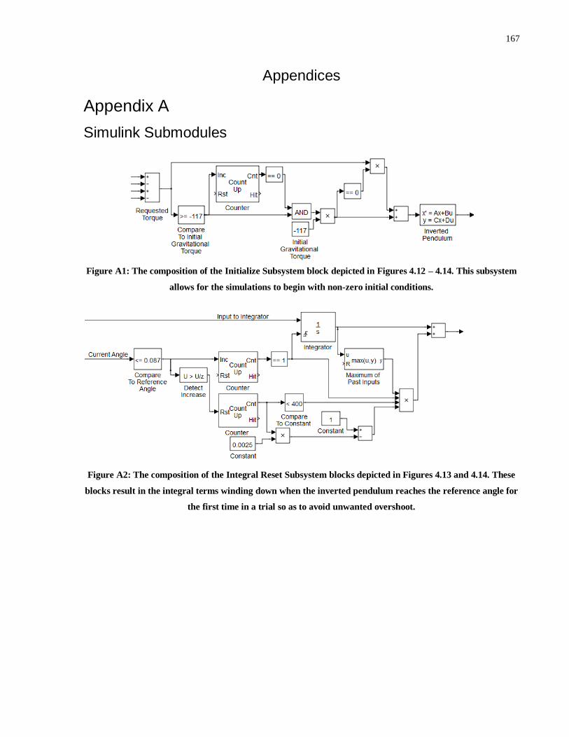
167
Appendices
Appendix A
Simulink Submodules
Figure A1: The composition of the Initialize Subsystem block depicted in Figures 4.12 – 4.14. This subsystem
allows for the simulations to begin with non-zero initial conditions.
Figure A2: The composition of the Integral Reset Subsystem blocks depicted in Figures 4.13 and 4.14. These
blocks result in the integral terms winding down when the inverted pendulum reaches the reference angle for
the first time in a trial so as to avoid unwanted overshoot.

168
Appendix B
Experiment 2 Calibration Curves

169

170
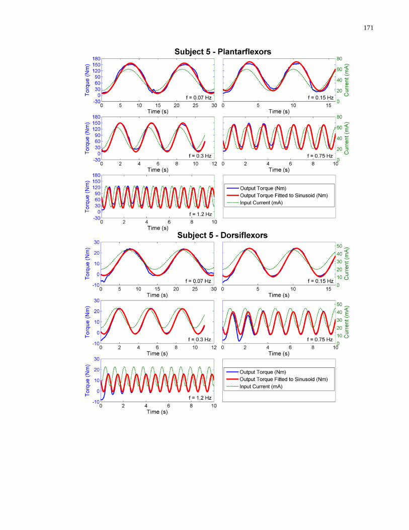
171

172

173
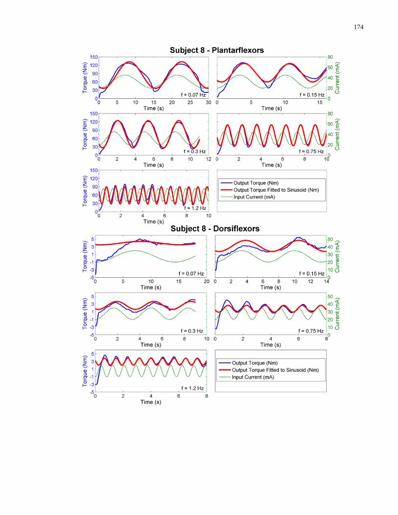
174
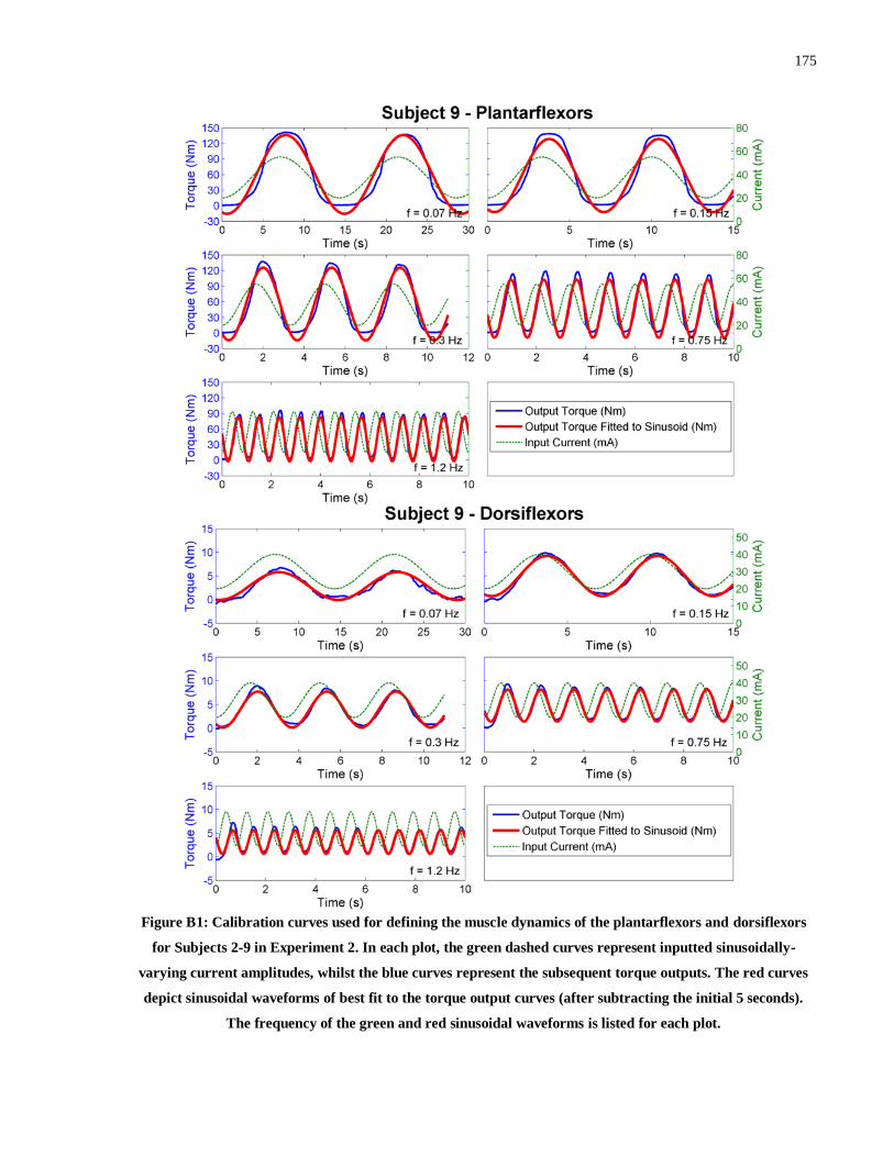
175
Figure B1: Calibration curves used for defining the muscle dynamics of the plantarflexors and dorsiflexors
for Subjects 2-9 in Experiment 2. In each plot, the green dashed curves represent inputted sinusoidally-
varying current amplitudes, whilst the blue curves represent the subsequent torque outputs. The red curves
depict sinusoidal waveforms of best fit to the torque output curves (after subtracting the initial 5 seconds).
The frequency of the green and red sinusoidal waveforms is listed for each plot.