Close-Out Risk Evaluation (CORE)

Close-Out Risk Evaluation (CORE)

Managing Simultaneously Liquidity and Market Risk for Central Counterparties

Marco Avellaneda, Courant Institute NYU Partner, Finance Concepts

Summary

1. Clearing

2. Close-Out Risk Evaluation (CORE)

3. Studies On Sample Portfolios

4. Conclusions

Clearing

Central clearing as a financial network

CM1

CM2

CM3

CM4

CM5

CM6 CM7

CCP

Clearing members: large banks, BDs Arrows represent credit exposure Small circles: non-clearing market participants (e.g., hedge funds, asset-managers, derivatives end-users, clients of CPs, retail investors)

Central clearing is a specific type of ``financial network’’ as in Hamini, Cont & Minca (2010)

Major Clearing Houses Today

Inter bank payments: ACH Securities: DTCC, FICC, LCH.Clearnet, Eurex Clearing Derivatives: CME Group, LCH.Clearnet, Intercontinental Exchange (ICE), ICE Clear Europe Options: The Options Clearing Corporation In Brazil, BM&F Bovespa manages 4 CCPs for different asset classes (like CME Group, which clears commodities, financials, and some OTC)

Tools for Risk Management of CCPs • Initial Margin is collected from CPs to cover extreme but plausible market shocks • Fund for mutualization of losses (``Guarantee Fund’’), covering shortfall beyond the IM • ``Loss tranches’’ which can be used to cover mutualized losses with CCP’s own capital ( Skin in the game)

BIS, Principles for Financial Markets Infrastructures, BIS CPSS-IOSCO Consultative Report, April 2012 ESMA, Final Report, Technical Standards on OTC Derivatives, CCPs and Trade Repositories (``EMIR’’), September 2012

Theoretical Risk Waterfall

Initial Margin (CMs)

CCP Tranche I

Guarantee Fund (CMs)

CCP Tranche II

Additional assessments to CMs

Important Research Problems

• Balance systemic risk requirements with costs involved for CMs.

• How much capital should go to IM and how much to the Guarantee Fund (mutualization of losses)? • Should there be more than 1 Clearing House for the same product in the same jurisdiction? • If so, should there be margin arrangements for netting exposures across CCPs (`interoperability’)? • How can CCPs generate synergies by using a common risk-management system to clear different products with the same risk factors (e.g. listed and OTC derivatives)?

My talk will deal with the last problem

Merging Central Counterparties

• NY Portfolio Clearing (NYPC): joint margining for Eurodollar and UST derivatives and FICC-cleared fixed income products (T-bonds, FMNA, repos) Joint venture between NYSE and FICC • BM&F Bovespa: after merging the stock exchange and the commodities and futures exchange, the group controls 4 different clearing platforms Derivatives (listed and OTC) Equities and stock loan Government Securities Foreign exchange

The BM&F Bovespa clearing system

Client

lLi Listed Deriv.

OTC Deriv.

Equities, Securities Lending

Bonds FX

10,000 Derivatives Accounts 500,000 Equities Accounts Ultimate beneficiary system – all accounts are subject to BM&F Bovespa margin not just broker-dealers

collateral collateral

collateral collateral

New risk-architecture for BM&F Bovespa

collateral

Listed & OTC derivatives Equities & stock loan bonds, FX

Client Objective: One margin methodology to cover all cleared products Challenges: • Many different risk factors

• Different liquidity profiles for securities (T+1, T+2, T+3, auctions) • Computationally intensive

Close-Out Risk Evaluation

Margin Methodology: Close-Out Risk Evaluation (CORE)

• Determine a suitable liquidation strategy for all instruments in portfolio of interest • Compute potential uncollateralized losses associated with liquidation of a portfolio under stress

BM&FBOVESPA’s Post-Trade Infrastructure: Integration Opportunities and Challenges, September 2010, www.bmf.com.br/bmfbovespa/pages/boletim2/informes/2010/marco/WhitePaper.pdf Paul Embrechts, Resnik and Samodorinski, Extreme Value Theory as a Risk Management Tool, N. American Actuarial J., 1999 Almgren, R and Neil Chriss, Optimal Execution of Portfolio Transactions, J. RISK, 2000

Market risk and liquidity risk

• To manage risk exposures, it is not enough to look just at market risk (VaR, SPAN) • Liquidity is essential

• This is manifested in the difference between unrealized, or mark-to-market, P/L and realized P/L after unwinding a position under distress • LTCM (1998): basis trades (long high spreads/short low spreads, DV01=0) • J.P. Morgan CIO (2012): basis trade, index CDS versus corporate CDS (2bb loss -> 8 bb loss)

• MF Global (2012): 2y term repos on Italian government bonds

• Grupo Interbolsa (2012) : Fabricato share repos, collapse of 2nd largest Colombian broker-dealer

Modeling portfolios with liquidity constraints

• In a world with infinite liquidity, a portfolio is represented as a list of instruments and quantities • In a world with limited liquidity, we should include the maximum amounts that can be traded in a given period (day) without `moving the market’*

* Proxied here at 10 % Avg. Traded Volume ** Guararapes Confecc. SA

Portfolio Description

• R represents the state of the market or path of states of the market (risk-factor changes)

• Example: if we are dealing with options, then 𝑅𝑡 =

𝑆𝑡𝜎𝑡𝑟𝑡𝑑𝑡

• represent quantities and daily liquidity limits for each instrument

𝑹 = 𝑅0, 𝑅1, 𝑅2, …𝑅𝑡 , 𝑅𝑡+1, …

Und. Price Volatility Interest rate Dividend yield

The Risk-factors

𝑄𝑖,𝑙𝑖

Liquidation of a Portfolio: `Close-out strategy’

• On date t=0, you decide that a portfolio should be liquidated starting on t=1. • Determine a strategy in which a certain fraction, 𝑞𝑖𝑡, of the of the position in instrument i will be liquidated at date t. ( 𝑞𝑖𝑡 , 𝑖 = 1,… , 𝑁, 𝑡 = 1,… , 𝑇𝑚𝑎𝑥)

• A close-out strategy is a matrix that tells us how to proceed for liquidating the various instruments in the portfolio as time passes.

0 ≤ 𝑞𝑖𝑡 ≤𝑙𝑖

𝑄𝑖≡ 𝑘𝑖 ∀𝑖 ∀𝑡

𝑞𝑖𝑡 = 1

𝑇𝑚𝑎𝑥

𝑡=1

𝑛𝑡 = 𝑞𝑠

𝑇𝑚𝑎𝑥

𝑠=𝑡+1

The remaining balance (%) at time t

Is there an `optimal’ close out-strategy?

• Define optimal

• Robert Almgren & Neil Chriss, Optimal Execution of Portfolio Transactions, 2000

-- Consider the liquidation of a single stock position, with the purpose of minimizing risk- adjusted shortfall. Balance the ``price impact’’ with ``urgency in executing’’.

𝑈 𝑞 =𝐸 𝑞 +𝜆𝑉 𝑞

𝐸 𝑞 = α 𝑞𝑡2 ∴

𝑇𝑚𝑎𝑥𝑡=1 𝑉 𝑞 =𝛽𝜎2 𝑛𝑡

2𝑇𝑚𝑎𝑥𝑡=1

Penalty fn. (minimize)

𝛼~1/𝑘2=𝑄2/𝑙2 𝛽~𝑄2

% executed on date t % balance on date t

Qu

anti

ty t

hat

r

emai

ns

to t

rad

e

Time elapsed

Qu

anti

ty t

hat

r

emai

ns

to t

rad

e

Time elapsed

𝑛𝑡 = 𝑠𝑖𝑛ℎ Ω 1−𝜏

𝑠𝑖𝑛ℎ Ω 𝜏 =

𝑡

𝑇𝑚𝑎𝑥

Ω = 𝑇𝑚𝑎𝑥𝜆𝛽𝜎2

𝛼

Solution of Almgren-Chriss

If you want to minimize market risk, trade fast but incur more cost (price impact). If you are not risk-sensitive, trade slowly in equal amounts per time. This minimizes shortfall due to price impact. This can be cast as an optimization problem which gives a close-out strategy.

Message:

Liquidating Hybrid Portfolios

• AC is OK for linear assets (stocks, futures) and short liquidation times (i.e. mostly algorithmic trading). Usually implemented for single positions. (variance represents risk fairly well) • Portfolio liquidation for Listed/ OTC derivatives (options, futures, swaps,…) is non-trivial and very necessary. • Liquidity for OTC derivatives: CP risk / CCP auctions. • Challenges: leverage, multiple risk-factors, quantifying liquidity. • Very important in applications: close-out trades for products with common market risk-factors and different liquidity profiles. • Look for ``natural hedges’’ in the liquidation process

Example of synchronization: Liquid vs. illiquid stocks

Petrobras average trading volumes PETR4: 24 million shares/day ( assume D/L=3MM ) PETR3: 8 million shares/day ( ‘’ D/L=1MM ) Assume shares have the same price Portfolio: Long 40 MM PETR4, short 30MM PETR3

PETR4 (sell)

PETR3 (buy)

1

1

3 3 3 3 3 1 1 1 1 1 1 1 1 ------------------------ 1 1 1 1 1 1

1 1 1 1 1 1 1 1 1 1 1 1 ------------------------ 1 1 1 1 1 1

Day 5 30

Mkt. exposure: 10 MM PETR4 for 5 days PETR 4 ``hedges’’ PETR 3 MTM P/L during liquidation

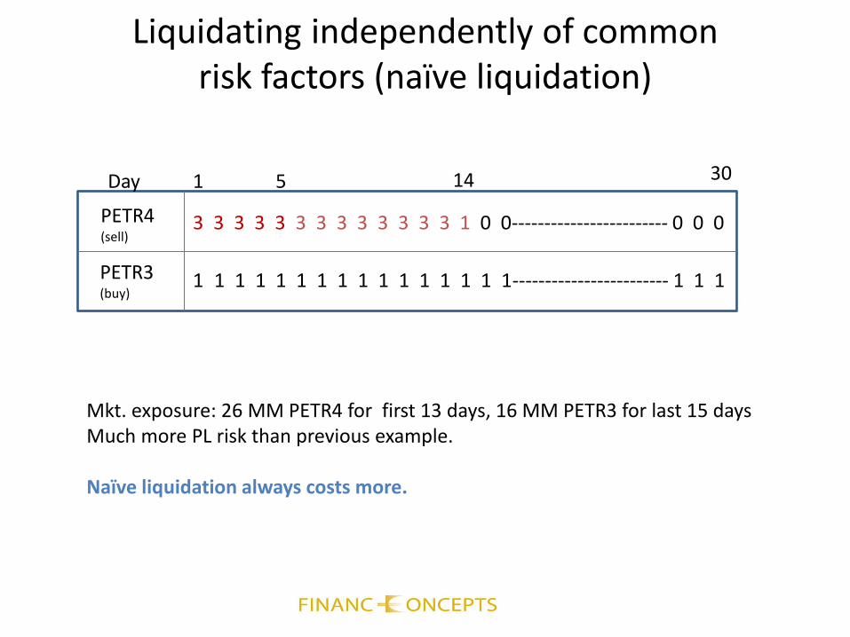
Liquidating independently of common risk factors (naïve liquidation)

PETR4 (sell)

PETR3 (buy)

1

1

3 3 3 3 3 3 3 3 3 3 3 3 3 1 0 0------------------------ 0 0 0

1 1 1 1 1 1 1 1 1 1 1 1 1 1 1------------------------ 1 1 1

Day 5 30

Mkt. exposure: 26 MM PETR4 for first 13 days, 16 MM PETR3 for last 15 days Much more PL risk than previous example. Naïve liquidation always costs more.

14

Profit and loss of a close-out strategy for a portfolio

𝜓𝑖 𝑡, 𝑅𝑡 ≝ 𝑄𝑖 𝑀𝑇𝑀𝑖 𝑡, 𝑅𝑡 −𝑀𝑇𝑀𝑖 0, 𝑅0

• Realized P/L at date t, after trading

• Unrealized (a.k.a. MTM) P/L at date t, after trading

𝐿𝑟 𝑡, 𝑞, 𝑅𝑡 = 𝑞𝑖𝑡𝜓𝑖 𝑡, 𝑅𝑡

𝑁

𝑖=1

P/L, full valuation

𝐿𝑛𝑟 𝑡, 𝑞, 𝑅𝑡 = 𝑛𝑖𝑡𝜓𝑖 𝑡, 𝑅𝑡

𝑁

𝑖=1

Accumulated P/L

• Accumulated profit/Loss for close out strategy at date t

𝐿 𝑡, 𝑞, 𝑅 = 𝐿𝑟 𝑠, 𝑞, 𝑅𝑠

𝑡

𝑠=1

+ 𝐿𝑛𝑟 𝑡, 𝑞, 𝑅𝑡

= 𝑞𝑖𝑠𝜓𝑖 𝑠, 𝑅𝑠

𝑁

𝑖=1

𝑡

𝑠=1

+ 𝑛𝑖𝑡𝜓𝑖 𝑡, 𝑅𝑡

𝑁

𝑖=1

cash unrealized gain/loss

Performance measures for close-out strategies

1. Final P/L:

• Sums all realized P/L in the course of liquidating the portfolio

• Ignores MTM profit/loss

𝐿 𝑇, 𝑞, 𝑅 = 𝐿𝑟 𝑡, 𝑞, 𝑅𝑡

𝑇𝑚𝑎𝑥

𝑡=1

= 𝑞𝑖𝑡𝜓𝑖 𝑡, 𝑅𝑡

𝑁

𝑖=1

𝑇𝑚𝑎𝑥

𝑡=1

Insensitive to intermediate P/L

Worst P/L & Average P/L

min1≤𝑡≤𝑇𝐿 𝑡, 𝑞, 𝑅

𝐿 𝑡, 𝑞, 𝑅 = 𝐿𝑟 𝑠, 𝑞, 𝑅𝑠

𝑡

𝑠=1

+ 𝐿𝑛𝑟 𝑡, 𝑞, 𝑅𝑡

𝑇𝑚𝑎𝑥

𝑡=1

𝑇𝑚𝑎𝑥

𝑡=1

2. Worst P/L

3. Average P/L (or sum)

L

t

L

t

Totally sensitive To intermediate P/L

Somewhat sensitive To intermediate P/L

Constructing the CORE objective function

• Define a set of extreme scenarios for the risk-factors

• These scenarios correspond to -- moves of spot prices

-- deformations of term-structures of interest rates and FX rate curves -- deformations of implied volatility surfaces -- deformations of credit spread curves… • Objective functions will correspond to worst-case losses under one of the preceding loss metric (terminal loss, worst loss, average loss) under extreme scenarios • Let 𝑹𝑒 denote the set of extreme scenarios for risk factors (a finite set in parameter space)

Objective Function #1: Terminal P/L

𝑈1 𝑞 = min𝑅𝐿 𝑇𝑚𝑎𝑥, 𝑞, 𝑅

= 𝑚𝑖𝑛𝑅 𝑞𝑖𝑡𝜓𝑖 𝑡, 𝑅𝑡

𝑁

𝑖=1

𝑇𝑚𝑎𝑥

𝑡=1

= min𝑅𝑡∈𝑹𝑒

𝑞𝑖𝑡𝜓𝑖 𝑡, 𝑅𝑡

𝑁

𝑖=1

𝑇𝑚𝑎𝑥

𝑡=1

We assume that the path of extreme scenarios can take any value on any date: ``zig-zag’’ scenarios.

Objective function #2: worst P/L

𝑈2 𝑞 = min𝑅min1≤𝑡≤𝑇𝑚𝑎𝑥

𝐿 𝑡, 𝑞, 𝑅

= min1≤𝑡≤𝑇𝑚𝑎𝑥

min𝑅 𝐿 𝑡, 𝑞, 𝑅


min𝑅 𝑞𝑖𝑠𝜓𝑖 𝑠, 𝑅𝑠

𝑁

𝑖=1

𝑡

𝑠=1

+ 𝑛𝑖𝑡𝜓𝑖 𝑡, 𝑅𝑡

𝑁

𝑖=1


min𝑅𝑠∈𝑹𝑒 𝑞𝑖𝑠𝜓𝑖 𝑠, 𝑅𝑠

𝑁

𝑖=1

𝑡−1

𝑠=1

+ min𝑅𝑡∈𝑹𝑒 𝑞𝑖𝑡 + 𝑛𝑖𝑡 𝜓𝑖 𝑡, 𝑅𝑡

𝑁

𝑖=1

Use zig-zag again

Objective Function #3: ``Average Loss’’

𝑈3 𝑞 = min𝑅𝑠∈𝑹𝑒 𝑞𝑖𝑠𝜓𝑖 𝑠, 𝑅𝑠

𝑁

𝑖=1

𝑡−1

𝑠=1


𝑁

𝑖=1

𝑇𝑚𝑎𝑥

𝑡=1

= (𝑇𝑚𝑎𝑥 − 𝑡) min𝑅𝑡∈𝑹𝑒 𝑞𝑖𝑡𝜓𝑖 𝑡, 𝑅𝑡

𝑁

𝑖=1


𝑁

𝑖=1

𝑇𝑚𝑎𝑥

𝑡=1

% liquidated on date t % balance on date t

Note: this is the closest to Almgren and Chriss. Can be viewed as an `` 𝐿1 version ‘’ of AC.

The Optimization Problem

Maximize Subject to:

𝑈𝑗 𝑞 𝑞 = 𝑞𝑖𝑡 ∈ 𝑅𝑁×𝑇𝑚𝑎𝑥



𝑞𝑖𝑡 = 1

𝑇𝑚𝑎𝑥

𝑡=1

∀𝑖

• U(q) is a sum of minima of linear functions of q => it is concave • The set of constraints is convex (it is a convex polyhedral region)

A solution exists and should be unique under reasonable conditions!

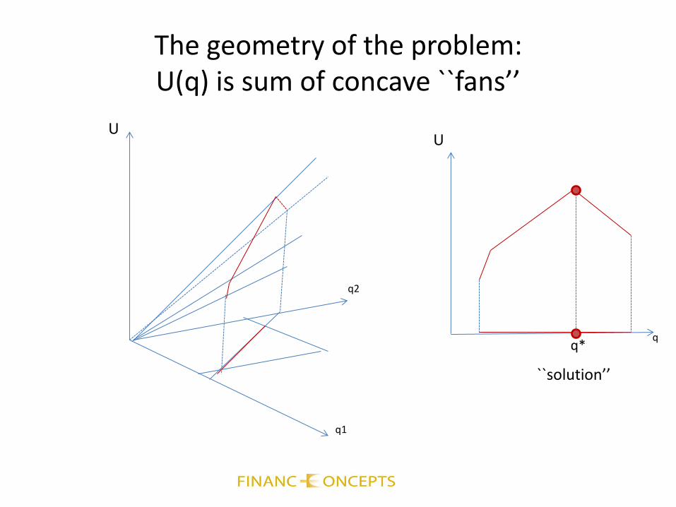
The geometry of the problem: U(q) is sum of concave ``fans’’

U

q1

q2

q

U

q*

``solution’’

Solution Via Linear Programming (LP)

Maximize: Over: Subject to:

𝑈3 = 𝑇𝑚𝑎𝑥 − 𝑡 𝜆𝑡 + 𝜇𝑡

𝑇𝑚𝑎𝑥

𝑡=1

𝜆𝑡 ≤ 𝑞𝑖𝑡𝜓𝑖 𝑡, 𝑅𝑡 ∀𝑡 ∀𝑅𝑡 ∈ 𝑹𝑒

𝑁

𝑖=1

𝜆𝑡, 𝜇𝑡 , 𝑞𝑖𝑡; 1 ≤ 𝑡 ≤ 𝑇𝑚𝑎𝑥, 1 ≤ 𝑖 ≤ 𝑁

𝜇𝑡 ≤ 𝑞𝑖𝑡 + 𝑛𝑖𝑡 𝜓𝑖 𝑡, 𝑅𝑡 ∀𝑡 ∀𝑅𝑡 ∈ 𝑹𝑒

𝑁

𝑖=1



𝑞𝑖𝑡 = 1

𝑇𝑚𝑎𝑥

𝑡=1

∀𝑖

𝑈1 = 𝜆𝑡

𝑇𝑚𝑎𝑥

𝑡=1

A theoretical result: Terminal Loss = Worst Loss

• Under mild assumptions which are reasonable in practice,

• Intuition: delaying realizing losses can only make things worse in extreme market conditions • Under worst-case scenarios, don’t expect make up losses one day by gains in the future • 𝑈3 𝑞 is different because it involves MTM P/L . In this case, delaying trading could be beneficial if it protects against MTM losses.*

max𝑞𝑈1 𝑞 =max

𝑞𝑈2 𝑞

* We like this.

Sample Portfolios

Practical Studies

We analyzed a variety of model portfolios. A few are presented here. • Instruments: derivatives traded at BM&F Bovespa (DOL, DI, etc,…)

• Listed Futures & Options

• OTC Forwards and Options

• Some OTC barrier options (not described here) Risk factors: 1. dolar spot (DOL) USD-BRL 2. cupom cambial Onshore carry 3. taxa pre-fixada (PRE) Yield curve 4. DOL volatility surface Vol surface

Test Portfolio #1: OTC forward vs. listed futures

Simbolo Produto Exercicio Vencimento Quantidade T+k Liquidez diaria

DOL1 f 63 2000 2 500

DOL1_call c 1.62 252 -2000 15 2000

DOL1_put p 1.62 252 2000 15 2000

• Long 2000 DOL Futures, expiration= 63 days, 1st trade= T+2, daily liquidity=500 • Short 2000 1.62 DOL Calls, expiration=252 days, 1st trade= T+15, daily liquidity= 2000 • Long 2000 1.62 DOL Puts, expiration=252 days, 1st trade= T+15, daily liquidity= 2000

Equivalent to: • Long 2000 DOL Futures, 1st trade=T+2, short 2000 DOL forwards, 1st trade T+15 (auction)

𝑈1(q)

P/L

Naïve (fast)

𝑈1(q) 𝑈3(q)

𝑈3(q)

Worst-case Profit/Loss

Test Portfolio #1

Test Portfolio #2

• Long 2,000 listed futures • Long 2,000 listed synthetic forwards (conversions) • Short 2,000 OTC forwards

Limited daily liquidity

1-day auction T+15

COREV1=CORE V3 CORE V2

Dia Fut (63) Call(63) Put(63) Call(252) Put(252) Fut (63) Call(63) Put(63) Call(252) Put252)

t+1 0 0 0 0 0 0 0 0 0 0

t+2 500 500 (500) 0 0 500 500 (500) 0 0

t+3 500 500 (500) 0 0 500 297 (500) 0 0

t+4 500 500 (500) 0 0 0 0 (345) 0 0

t+5 0 0 0 0 0 0 0 (7) 0 0

t+6 0 0 0 0 0 0 0 (7) 0 0

t+7 0 0 0 0 0 0 0 (7) 0 0

t+8 0 0 0 0 0 0 0 (7) 0 0

t+9 0 0 0 0 0 0 0 (6) 0 0

t+10 0 0 0 0 0 0 0 (6) 0 0

t+11 0 0 0 0 0 0 0 (6) 0 0

t+12 0 0 0 0 0 0 0 (6) 0 0

t+13 0 0 0 0 0 0 203 0 0 0

t+14 0 0 0 0 0 500 500 (103) 0 0

t+15 500 500 (500) (2000) 2000 500 500 (500) (2000) 2000

CORE V3.1

Dia Fut (63) Call(63) Put(63) Call(252) Put(252)

t+1 0 0 0 0 0

t+2 500 0 0 0 0

t+3 500 0 (0) 0 0

t+4 0 (0) 0 0 0

t+5 0 0 0 0 0

t+6 (0) 0 (0) 0 0

t+7 0 0 (0) 0 0

t+8 (0) 0 (0) 0 0

t+9 0 (0) (0) 0 0

t+10 0 0 0 0 0

t+11 (0) 0 0 0 0

t+12 (0) 500 (500) 0 0

t+13 (0) 500 (500) 0 0

t+14 500 500 (500) 0 0

t+15 500 500 (500) (2000) 2000

𝑈1(q)

𝑈3(q) 𝑈1(q)

𝑈3(q)

Naive

Test Portfolio #2

Test Portfolio #3


DOL1 f 63 2000 2 500

DOL1_call c 1.62 63 2000 2 500

DOL1_put p 1.62 63 -2000 2 500

DOL1_call c 1.62 250 2000 2 500

DOL1_put p 1.62 250 -2000 2 500

DOL1_call c 1.62 252 -2000 15 2000

DOL1_put p 1.62 252 2000 15 2000

• Long 2,000 listed futures • Long 2,000 listed conversions (expiration=63) • Long 2,000 listed conversion (expiration=250) • Short 2,000 OTC forwards (expiration= 252)

Limited daily liquidity

Settle in auction in T+15

𝑈1(q)

𝑈3(q)

Test Portfolio #3

𝑈1(q)

𝑈3(q)

Naive

Test Portfolio #4


DOL1 f 63 4000 2 500

DOL1_call c 1.62 252 -2000 15 2000

DOL1_put p 1.62 252 2000 15 2000

• Long 4,000 listed futures D/L = 500 T+2

• Short 2,000 OTC forwards T+15 auction

𝑈1(q)

𝑈3(q)

Worst P/L*

𝑈1(q)

𝑈3(q)

naive

Test Portfolio #4

* Pink is a suboptimal strategy which we do not analyze here

Test Portfolio #5


DOL1 f 63 2000 2 500

DOL1_call c 1.62 252 -2000 15 2000

DOL1_put p 1.62 252 -2000 15 2000

• Long 2000 listed futures D/L=500, T+2

• Short 2,000 OTC Straddles T+15 auction

CORE V1/V3 CORE V2

Dia Fut (63) Call(252) Put(252) Fut (63) Call(252) Put(252)

t+1 0 0 0 0 0 0

t+2 500 0 0 500 0 0

t+3 500 0 0 500 0 0

t+4 500 0 0 45 0 0

t+5 0 0 0 0 0 0

t+6 0 0 0 0 0 0

t+7 0 0 0 0 0 0

t+8 0 0 0 0 0 0

t+9 0 0 0 0 0 0

t+10 0 0 0 0 0 0

t+11 0 0 0 0 0 0

t+12 0 0 0 0 0 0

t+13 0 0 0 0 0 0

t+14 0 0 0 453 0 0

t+15 500 (2000) (2000) 500 (2000) (2000)

CORE V3.1

Dia Fut (63) Call(252) Put(252)

t+1 0 0 0

t+2 500 0 0

t+3 500 0 0

t+4 45 0 0

t+5 0 0 0

t+6 0 0 0

t+7 0 0 0

t+8 0 0 0

t+9 0 0 0

t+10 0 0 0

t+11 0 0 0

t+12 0 0 0

t+13 0 0 0

t+14 453 0 0

t+15 500 (2000) (2000)

𝑈1(q)

𝑈3(q)

Test Portfolio #5

𝑈1(q)

𝑈3(q)

naive

Worst P/L

Test Portfolio #6


DOL1 f 63 2000 2 500

DOL1_call c 1.62 63 2000 2 500

DOL1_put p 1.62 63 2000 2 500

DOL1_call c 1.62 252 -2000 15 2000

DOL1_put p 1.62 252 -2000 15 2000

• Long 2000 listed futures D/L=500 • Long 2000 listed straddles D/L=500 • Short 2000 OTC straddles T+15 auction

COREV1=CORE V3 CORE V2

Dia Fut (63) Call(63) Put(63) Call(252) Put(252) Fut (63) Call(63) Put(63) Call(252) Put252)

t+1 0 0 0 0 0 0 0 0 0 0

t+2 479 0 500 0 0 500 0 0 0 0

t+3 479 0 500 0 0 401 0 0 0 0

t+4 390 0 500 0 0 8 0 0 0 0

t+5 152 0 196 0 0 1 0 0 0 0

t+6 0 0 0 0 0 1 0 0 0 0

t+7 0 0 0 0 0 1 0 0 0 0

t+8 0 0 0 0 0 0 0 0 0 0

t+9 0 0 0 0 0 0 0 0 0 0

t+10 0 0 0 0 0 0 0 0 0 0

t+11 0 0 0 0 0 0 0 0 0 0

t+12 0 500 104 0 0 291 500 500 0 0

t+13 0 500 101 0 0 23 500 500 0 0

t+14 0 500 98 0 0 274 500 500 0 0

t+15 500 500 0 (2000) (2000) 500 500 500 (2000) (2000)

CORE V3.1

Dia Fut (63) Call(63) Put(63) Call(252) Put(252)

t+1 0 0 0 0 0

t+2 500 0 443 0 0

t+3 0 0 0 0 0

t+4 0 0 0 0 0

t+5 0 0 0 0 0

t+6 0 0 0 0 0

t+7 0 0 0 0 0

t+8 0 0 0 0 0

t+9 0 0 0 0 0

t+10 0 0 0 0 0

t+11 46 0 57 0 0

t+12 319 500 500 0 0

t+13 323 500 500 0 0

t+14 312 500 500 0 0

t+15 500 500 0 (2000) (2000)

naive

𝑈1(q)

𝑈3(q)

𝑈3(q)

𝑈1(q) 𝑈3(q)

naive

Test Portfolio #6

Worst P/L*

Test Portfolio #7


DOL1 f 63 2000 2 500

DOL1_call c 1.62 63 2000 2 500

DOL1_put p 1.62 63 2000 2 500

DOL1_call c 1.62 220 2000 2 500

DOL1_put p 1.62 220 2000 2 500

DOL1_call c 1.62 252 -2000 15 2000

DOL1_put p 1.62 252 -2000 15 2000

• Long 2000 dollar futures expiration 3 months • Long 2000 50-delta calls “ 3 months • Long 2000 50-delta straddles ‘’ 220 days • Short 2000 40-delta straddles ‘’ 252 days

D/L=500, T+2

Auction in T+15

𝑈1(q)

𝑈3(q)

Worst P/L

𝑈1(q) 𝑈3(q)

naive

Test Portfolio #7

Conclusions

Analysis: comparing worst-case scenario losses

Portfolio Naïve liquidation

𝑼𝟑 𝒒 a.k.a. CORE

Improvement

1 1,322 1,053 21%

2 1,869 1,298 31%

3 2,476 1,541 38%

4 1,913 1,621 16%

5 1,246 947 24%

6 943 451 53%

7 990 332 68%

Futures vs. OTC forwards

OTC/Listed w/ options

• Using this technique should improve margin requirements for portfolios in CCP clearing!

Final Remarks • We presented a general formulation of the problem of liquidating portfolios of derivative securities and its solution. • The approach incorporates: -- liquidity limits for instruments -- MTM functions depending on risk-factors -- extreme scenarios for risk-factors. • The solution is found by solving a linear programming optimization problem. • The approach is conceptually simple -- it associates and synchronizes the liquidation of instruments with common risk factors, taking account explicitly varying degrees of liquidity. • It can be viewed as a cross-asset, liquidity-adjusted SPAN. • It is the computational engine of BM&F Bovespa’s new Post-Trade Infrastructure framework.

Acknowledgements

This work was done in collaboration between Finance Concepts and BM&F Bovespa.

Special thanks and credit to

BM&F Bovespa Finance Concepts Cicero Vieira Rama Cont Luis Vicente Baron Guerra Hao Yao Tatiana Iwashita Joffrey Grizard Fernando Valvano Cerezetti Silvio Rodriguez de Faria Alan de Genaro

Close-Out Risk Evaluation (CORE)

Documents

Transcript of Close-Out Risk Evaluation (CORE)