Clocks, Power and Synchronization in Duty-Cycled Wireless

FACTA UNIVERSITATIS (NIS)

SER.: ELEC. ENERG. vol. 24, no.2, August 2011, 183-208

Clocks, Power and Synchronization in Duty-CycledWireless Sensor Nodes

Dedicated to Professor Slavoljub Aleksic on the occasion of his 60th birthday

Mile K. Stoj cev, Ljubisa R. Golubovic,and Tatjana R. Nikoli c

Abstract: Recent advances in CMOS VLSI ICs and micro-electromechanical tech-nology have led to development of small, low-cost, and low-power multifunctionalsensors. Wireless sensor networks (WSNs) are large-scale networks of such sensors,dedicated to observing and monitoring various aspects of the physical world. Some in-trinsic properties of WSNs including limited resource of energy, storage, computation,and bandwidth, make traditional synchronization methods unsuitable for WSNs. Timesynchronization as an important issue consists of giving all sensor nodes (SNs) of theWSN a common time scale to operate. The common time scale is usually achieved byperiodically synchronizing the clock of each SN to a reference source. In this mannerthe local time seen by each SN of the network is approximatelythe same, and timesynchronization allows the entire system to cooperate. This paper gives a brief look tothe time synchronization problem and the need for synchronization in WSNs. Then itpoints out that clock systems become a bottle-neck, after that it presents the availablecurrent clock technologies, next it examines the influence of these clock technolo-gies, and finally provides guidelines for WSN developers who must choose among thedifferent clock synchronization techniques.

Keywords: Wireless sensor network; clock synchronization; duty-cycled wirelesssensor nodes.

Manuscript received on May 25, 2011.M. Stojcev and T. Nikolic are with University of Nis, Faculty of Electronic Engi-

neering, Aleksandra Medvedeva 14, 18000 Nis, Serbia (e-mails:[mile.stojcev,tatjana.nikolic]@elfak.ni.ac.rs). Lj. Golubovic is with University ofKragujevac, Technical FacultyCacak, Svetog Save 65, 32000Cacak, Serbia (e-mail:[email protected]).

183

184 M. Stojcev, Lj. Golubovic, and T. R. Nikolic:

1 Introduction

DURING the last two decades, tremendous technological advances have oc-curred in the development of low cost sensors, which are capable of wireless

communication and data processing. Wireless sensor networks (WSNs) are dis-tributed networks of such sensors, dedicated to closely observing real-word phe-nomena [1,2].

One of the biggest challenges for designers of WSNs is to develop systemsthat will run unattended for years. The current generation of sensornodes (SNs) isbattery powered, so lifetime is a major constraint; future generations powered byambient energy sources (sunlight, vibrations, etc), will provide very lowcurrents,so energy consumption is heavily constrained [3].

In addition, efficient coordination of SNs requires the nodes to be synchronized,so the nodes can be turned off to save energy. The purpose of any time synchroniza-tion technique is to maintain a similar time within a certain tolerance throughoutthe lifetime of the network or among a specific set of nodes in the network. Theproblem consists of giving all the nodes of the network a common time scale tooperate: time measurements, coordinated actions and event ordering require com-mon time on WSN nodes. Due to intrinsic energy limitations of wireless networksthere is a need for energy-efficient time synchronization solutions, different fromthe ones have been developed for wired networks. In this work we investigated thetrade-offs between time synchronization accuracy and energy saving inWSNs. Thecommon time scale is usually achieved by periodically synchronizing the clock ateach node to a reference time source; therefore the local time seen by each elementof the system is approximately the same [4].

An understanding of the intrinsic interactions between the diffuse local clocksand their cumulative effect on network-wide performance is consideredin this pa-per. Over the last decade, most improvements were made in the synchronizationalgorithm trying to minimize message exchange and optimize radio architecturesto provide accurate time-stamping mechanisms [5]. The influences of the underly-ing clock system and its impact on the overall synchronization accuracy has largelybeen unstudied. Here, we concentrate on the problem of choosing the right clockand duty cycle for a sensor node with order to achieve correct synchronization andlong lifetime.

2 Clock Synchronization in WSNs

In centralized systems there is no need for synchronized time because there is notime ambiguity. Contrary to this, in distributed systems, such as WSNs, there is noglobal clock or common memory.

Clocks, Power and Synchronization in Duty-Cycled Wireless Sensor Nodes 185

In WSNs each processor in sensor node (SN) has its own internal clockandits own notion of time. In practice, these clocks can easily drift second per day,accumulating significant errors over time, and thus potentially remaining unsyn-chronized.

For more applications and algorithms that run in WSN, we need to know moreabout time synchronization having in mind the following:

(a) The time of a day at which an event happened on a specific SN in the WSN.

(b) The time interval between two events happened on different SNs in the WSN.

(c) The relative ordering of events that happened on different SNs inthe WSN.

Clock synchronization in WSN is the process of ensuring that physically dis-tributed SNs have a common notion of time. There are three basic solutions fortime synchronization in WSN [5]:

1. One-way message dissemination: the simplest form of synchronization dealsonly with ordering of events or messages. Using this approach it is possibleto tell whether an eventE1 has occurred before or after another eventE2.

2. Receiver-receiver synchronization: SNs run their local clocks independently,but they keep information about the relative drift and offset of their clock toother clocks in the network.

3. Two way message exchange: the most complex form of synchronizationcalled “always on” model, where all SNs maintain a clock that is synchro-nized to a reference clock in the network.

3 Clocking Terminology

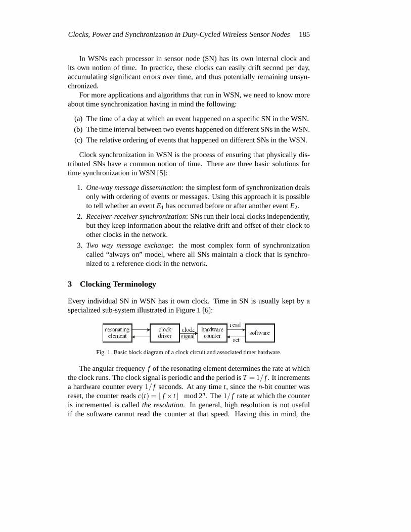
Every individual SN in WSN has it own clock. Time in SN is usually kept by aspecialized sub-system illustrated in Figure 1 [6]:

Fig. 1. Basic block diagram of a clock circuit and associated timer hardware.

The angular frequencyf of the resonating element determines the rate at whichthe clock runs. The clock signal is periodic and the period isT = 1/ f . It incrementsa hardware counter every 1/ f seconds. At any timet, since then-bit counter wasreset, the counter readsc(t) = ⌊ f × t⌋ mod 2n. The 1/ f rate at which the counteris incremented is calledthe resolution. In general, high resolution is not usefulif the software cannot read the counter at that speed. Having this in mind, the


smallest increment at which an application can read a counter is calledprecision.The counter is typically set to an Universal Time Calendar, UTC. The accuracydetermines how true the counter is close to that calendar [6]

For any two clocksCa andCb, we will point to the used terminology which isconsistent with definitions given in [7].

Time: The time of a clock in a SNp is given by the functionCp(t) = t for aperfect clock.

Frequency: Frequency is the rate at which a clock progresses. The frequencyat timet of the clockCa is C′

a(t).

Offset: Clock offset is the difference between the time reported by a clock andthe real time. The offset of the clockCa is given byCa(t). The offset of clockCa

relative to clockCb at timet ≥ 0 is given byCa(t)−Cb(t).

Skew: The skew of a clock is the difference in the frequencies of the clockand the perfect clock. The skew of a clockCa relative to clockCb at time t isC′

a(t)−C′b(t).

If the skew is bounded byρ, then as per eq. (1), clock values are allowed todiverge at a rate in the range of 1−ρ to 1+ρ.

Drift (rate) : The drift of clockCa is the second derivative of the clock valuewith respect to time, namelyC′′

a . The drift of clockCa relative to clockCb at timetis C′′

a(t)−C′′b(t).

Due to clock inaccuracy the clock is said to be working within its specification

1−ρ ≤dCd t

< 1+ρ (1)

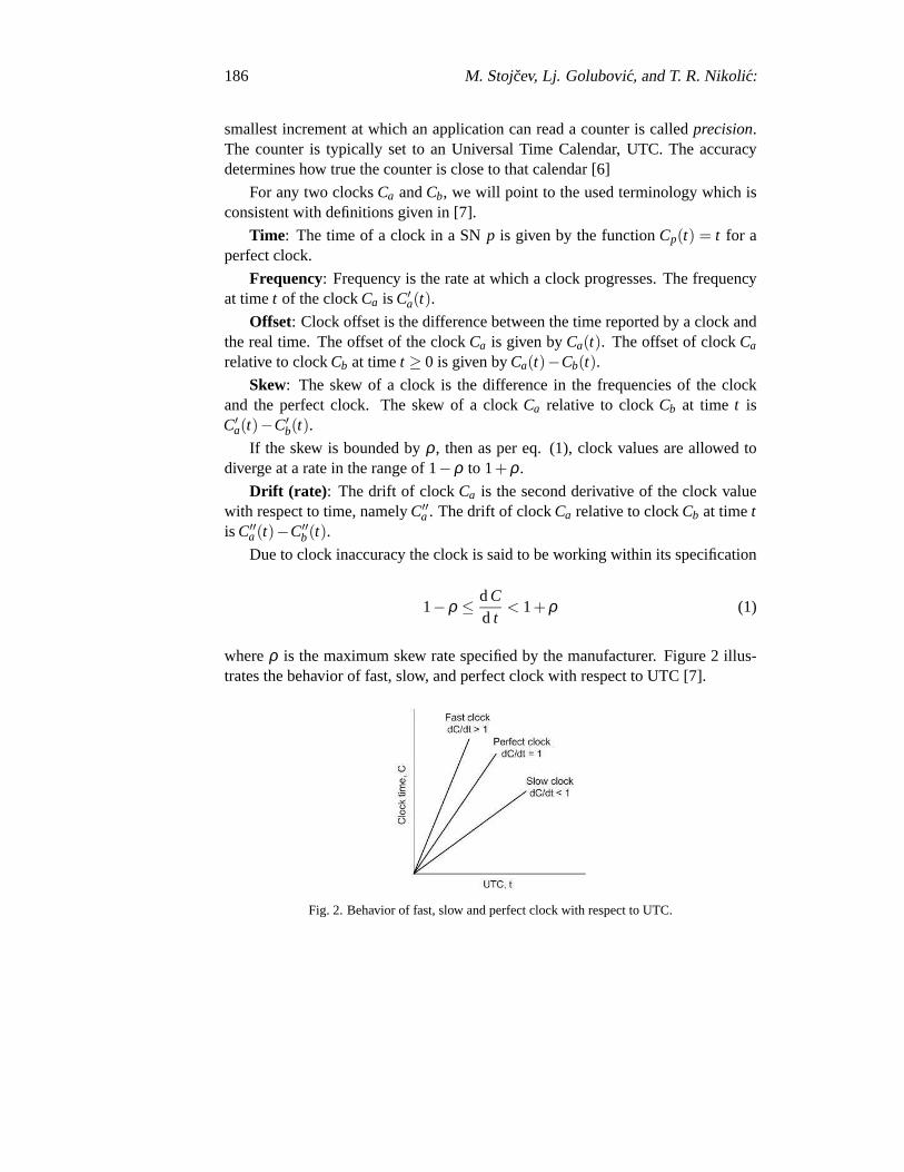
whereρ is the maximum skew rate specified by the manufacturer. Figure 2 illus-trates the behavior of fast, slow, and perfect clock with respect to UTC [7].

Fig. 2. Behavior of fast, slow and perfect clock with respect to UTC.


Equation (1) can be transformed into:

(1−ρ)∆t ≤∆C < (1+ρ)∆t (2)

∆C1+ρ

≤∆t <∆C

1−ρ(3)

It can be inferred that the local clock difference∆C that corresponds to thereal-time difference∆t can be bounded by the following interval:

[(1−ρ)∆t, (1+ρ)∆t] (4)

4 Sender to Receiver Synchronization

One standard technique to deal with clock uncertainty is to estimate the frequencyerror of the local clock. The following two factors, manufacturing inaccuracies andchanges in environmental temperature, are the two major contributors to clockun-certainties. While manufacturing imprecision is static over the lifetime of a compo-nent, changes in environmental temperature require frequent recalibration. In addi-tion, problems in clock synchronization occur because uncertainties are introducedby the wireless channel, too. Deep fading, interference, unpredictablelatencies dueto the broadcast nature of the wireless channel, and higher bit error rates, than inwired networks, all complicate synchronization efforts.

We use traditional sender-to-receiver synchronization which usually happens inthe following three steps:

1. The sender node periodically sends a message with its local time as a time-stamp to the receiver.

2. The receiver then synchronizes with the sender using the time-stamp it re-ceives from the sender.

3. The message delay between the sender and receiver is calculated.

Most majority methods synchronize a sender with a receiver by transmittingthe current clock values as time-stamps. We call this kind of synchronizationasone-way message dissemination.

5 Main Characteristics of WSNs

The basic operation of WSNs is data fusion. In spite of that data fusion requiresthat SNs be synchronized. The synchronization protocols for WSNs must addressthe following features of these networks [7]:


Limited energy: WSNs can employ thousands of battery-powered SNs. Sincethe amount of energy available to such sensors is quite modest, synchronizationmust be achieved, while data processing is active with order to utilize these sensorsin an efficient fashion.

Limited bandwidth : in WSNs much less power is consumed in processingdata than transmitting it. Bandwidth limitation directly affects message exchangesamong SNs, and synchronization is impossible without message exchanges.

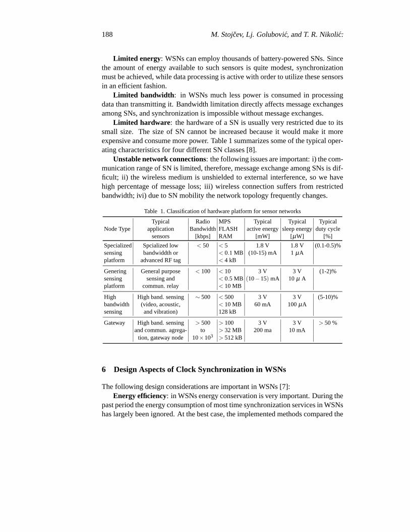
Limited hardware : the hardware of a SN is usually very restricted due to itssmall size. The size of SN cannot be increased because it would make it moreexpensive and consume more power. Table 1 summarizes some of the typicaloper-ating characteristics for four different SN classes [8].

Unstable network connections: the following issues are important: i) the com-munication range of SN is limited, therefore, message exchange among SNs is dif-ficult; ii) the wireless medium is unshielded to external interference, so we havehigh percentage of message loss; iii) wireless connection suffers from restrictedbandwidth; ivi) due to SN mobility the network topology frequently changes.

Table 1. Classification of hardware platform for sensor networks

Typical Radio MPS Typical Typical TypicalNode Type application Bandwidth FLASH active energysleep energyduty cycle

sensors [kbps] RAM [mW] [µW] [%]

Specialized Spcialized low < 50 < 5 1.8 V 1.8 V (0.1-0.5)%sensing bandwiddth or < 0.1 MB (10-15) mA 1 µAplatform advanced RF tag < 4 kB

Genering General purpose < 100 < 10 3 V 3 V (1-2)%sensing sensing and < 0.5 MB (10−15) mA 10 µ Aplatform commun. relay < 10 MB

High High band. sensing ∼ 500 < 500 3 V 3 V (5-10)%bandwidth (video, acoustic, < 10 MB 60 mA 100µAsensing and vibration) 128 kB

Gateway High band. sensing > 500 > 100 3 V 3 V > 50 %and commun. agrega- to > 32 MB 200 ma 10 mA

tion, gateway node 10×103 > 512 kB

6 Design Aspects of Clock Synchronization in WSNs

The following design considerations are important in WSNs [7]:Energy efficiency: in WSNs energy conservation is very important. During the

past period the energy consumption of most time synchronization services inWSNshas largely been ignored. At the best case, the implemented methods compared the


number of messages sent per synchronization exchange between SNs.While this isan important measure, other components of the hardware platform start to becomemuch more relevant in the power budget as communication overhead gets reduced.These overheads are particularly pronounced in the extremely low duty-cycles thatWSNs try to achieve. In such scenario, a high precision and high frequency clockcan quickly become the most significant energy consumer during sleep times,thusinvalidating any power gains made in synchronization accuracy.

Infrastructure : the SNs must cooperate to organize themselves into a networkand resolve contention for available bandwidth.

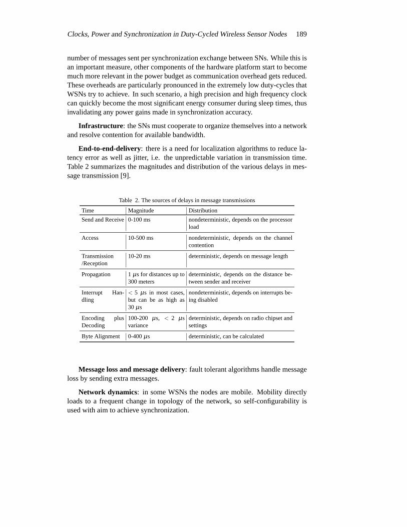
End-to-end-delivery: there is a need for localization algorithms to reduce la-tency error as well as jitter, i.e. the unpredictable variation in transmission time.Table 2 summarizes the magnitudes and distribution of the various delays in mes-sage transmission [9].

Table 2. The sources of delays in message transmissions

Time Magnitude Distribution

Send and Receive0-100 ms nondeterministic, depends on the processorload

Access 10-500 ms nondeterministic, depends on the channelcontention

Transmission/Reception

10-20 ms deterministic, depends on message length

Propagation 1 µs for distances up to300 meters

deterministic, depends on the distance be-tween sender and receiver

Interrupt Han-dling

< 5 µs in most cases,but can be as high as30 µs

nondeterministic, depends on interrupts be-ing disabled

Encoding plusDecoding

100-200 µs, < 2 µsvariance

deterministic, depends on radio chipset andsettings

Byte Alignment 0-400µs deterministic, can be calculated

Message loss and message delivery: fault tolerant algorithms handle messageloss by sending extra messages.

Network dynamics: in some WSNs the nodes are mobile. Mobility directlyloads to a frequent change in topology of the network, so self-configurability isused with aim to achieve synchronization.


7 Up-To-Date Methods of WSN Synchronization

There are several reasons for addressing synchronization problem in WSNs. Wewill point to two most important. First, SNs need to coordinate their operations andcollaborate to achieve a complex sensing task. Data fusion is an example of suchcoordination in which data collected at different SNs are aggregated into mean-ingful results. Second, synchronization can be used by power savingschemes toincrease network life-time. For example, SNs may sleep at appropriate time, andwake-up when necessary. When using power-saving nodes, the SNsshould sleepand wake-up at coordinated times, such that the radio receiver of SN is not turned-off when there is some data directed to it. This requires a precise timing betweenSNs. Many different methods of time synchronization are in common use today[4].

The well known synchronization protocols for wired networks, such asNet-work Time Protocol (NTP), Precision Time Protocol (PTP), IEEE 1588v2andIEEE 802.1AS are usually not suitable for WSNs due to limited hardware andenergy resources available on SNs [4, 10]. To bypass these problems, in recentyears, several WSN specific synchronization protocols have been proposed. How-ever most of them are focused on achieving high synchronization accuracy for thewhole network without addressing the power consumption problem. We will groupWSN time synchronization methods into the following three categories [10]: a)high accuracy; b) light-weight; and c) adaptive. A short description ofstandardprotocols that belong to each of the aforementioned groups follows:

a) High-accuracy synchronization methods- the following four protocols aretypical for this group.

a1) Time-Stamp Synchronization (TSS) protocol[11] - transforms thetime of one network node to the time of another node whenever theyexchange time-stamped radio messages. After the reception of a mes-sage with a time-stamp, the node estimates the time-stamp edge, andthen subtracts the time-stamp edge from the message arrival time. Theresult of this subtraction is the time-stamp value which corresponds tothe receiver time.

a2) Reference-Broadcast Synchronization (RBS) protocol[12] - a spe-cial reference node sends radio messages to its one-hop neighbors,which time-stamp the messages upon reception, and then exchange thetime-stamp values. Every node uses these values to compute instanta-neous relative offsets of its clock with respect to the clocks of the othernodes (excluding the reference node). The nodes compute their relativeclock drift rates by means of least-square linear regression.


a3) Timing-sync Protocol for Sensor Networks(TPSN) [13] - works intwo phases. During the first, called level discovery phase, a spanningtree is created in the network, i.e. to each node a level number is as-signed. At the start the root of the tree at level 0 broadcasts a leveldiscovery packet which contains the root ID and level number. Thenodes receive that packet and assign themselves a level number, greaterby one than the level number of the received packet. In the second,synchronization phase, the root broadcasts a special packet to initiatesynchronization.

a4) Flooding Time Synchronization Protocol(FTSP) [9] - floods the wholenetwork with messages, which contain values of the global time, i.e.the time of the elected leader. The synchronization leader periodicallybroadcasts synchronization messages containing its time-stamps. Anetwork node records its local time upon reception of a synchronizationmessage and forms a reference point, which contains global and localtime. When the node collects a sufficient number of referent points, itcomputes the drift rate of its clock with respect to the leader clock usinglinear regression.

b) Light-Weight Synchronization Methods - in general, accurate time syn-chronization needs more complex computations and more frequent networkcommunications, which leads to an increased energy consumption. In or-der to improve power efficiency by reducing the synchronization overheadrelated to communication and computation several efficient protocol are pro-posed [10].

b1) Tiny-Sync and Mini-Sync (TS/MS) protocol [14] - a hierarchy ofnetwork nodes exists where each parent and child can exchange time-stamped radio messages. In this case improvement of power efficiencyis achieved by reducing the synchronization complexity, and by enlarg-ing the synchronization period.

b2) Lightweight Tree-based Synchronization (LTS) scheme[15] - savespower by means of fewer radio messages and less complex computa-tions are necessary for the time synchronization. Two LTS algorithmsperform periodic synchronization by exchanging a pair of time stampedmessages along edges of a spanning tree. In the first, centralized algo-rithm, a reference node (i.e. root of the tree) synchronizes with itssingle hop neighbors, then they synchronize with their children, untilall leaf nodes of the tree are synchronized. In the second, distributedalgorithm, network nodes decide on their own whether they need to besynchronized. A node that requires synchronization sends a request to


the closest reference node.

c) Adaptive Synchronization Methods- TS/MS and LTS often include sep-arate ad hoc synchronization methods, each of which is the most suitablein certain scenario, depending on the required accuracy or number of ac-tive nodes in WSN. However these parameters can change rather quicklyinWSN [10]. Therefore it is desirable to have time synchronization schemesthat combine various specific algorithms and apply them selectively depend-ing on the situation. Such flexible techniques should be able to keep trackon variable conditions and synchronize the SNs in most energy-efficientway[10]. Some of the protocols which belong in this group are the following.

c1) Adaptive Time Synchronization (ATS) protocol [16] - uses the min-imum number of synchronization messages to achieve a required accu-racy with a certain probability. Each of the dedicated SNs sends time-stamped radio messages to a set of receivers. The receivers registerthe arrival time of those reference messages, and use linear regressionto compute the offset and drift rate of their clocks with respect to thesender clock. Then they send the computed values back to the sender,which uses this information to find its relative clock drift rate and tobroadcast it in a special packet to all receivers. After that, any pair ofreceivers can compute their relative clock drift rates and offsets.

c2) Energy Efficient Time Synchronization Protocol (ETSP)[17] - min-imizes the number of synchronizations, what depends on the numberof SNs requiring synchronization. This technique is based on the ob-servation that receiver-receiver synchronization (used in RBS) requiresless transmission than sender-receiver synchronization (used in TPSN)when the number of SNs is small. On the contrary, the sender-receiverapproach is more energy efficient in large and dense WSNs.

c3) Rate Adaptive Time Synchronization (RATS)[18] - multiplicativelydecreases and increases the synchronization interval within certain lim-its depending on how many times the synchronization error exceeds theuser-defined bound.

More details concerning the principles of operation of all three groups ofpro-tocols can be found in [7,10,19].

8 How to Prolong Lifetime of SN?

Lifetime refers to the time period for which a sensor network is capable of sensingand transmitting the sensed data to the base station(s). In WSNs, thousands of


nodes are powered with very limited supply of battery power. As a result, lifetimeanalysis becomes an important aspect to efficiently use the available energy. Insensor networks using rechargeable energy, such as solar energy, lifetime analysishelps the node to use energy efficiently before recharging. Lifetime analysis mayinclude an upper bound on the lifetime and factors influencing this upper bound[20].

Sensor networks should operate with the minimum possible energy to increasethe life of sensor nodes. This requires power aware computation/communicationcomponent technology, low-energy signaling and networking, and power awaresoftware communication. Design challenges encountered in the building of WSNscan be broadly classified into hardware, wireless networking, and OS/applications[3]. All three categories should minimize the power usage to increase the life of asensor node. Hardware includes the design activities related to all hardware plat-forms (MEMS, digital circuit design, system integration, and RF) that make upsensor networks. The second aspect includes design of power-efficient algorithmsand protocols (energy efficient protocols for MAC and routing like that discussedin the previous section). The third relates to power management in sensor nodes.Namely, additional power savings can be obtained by using Dynamic Power Man-agement (DPM). The basic idea behind DPM is to shutdown (sleep mode) the SNswhen not needed and get them back (wake up) when required. Our design solu-tion, presented in this paper, is based on combination of DPM with timer logic asprogrammable hardware unit.

9 Duty Cycling

In order to minimize the energy consumption of wireless sensor node differenttechniques for reducing power consumption are used [3]. Among them duty cyclinghas become a crucial one. The idea behind this is clear. Keep hardware ina lowpower sleep state except on the infrequent instances when the hardware is needed.In many design solutions this allows even the processor to be put into a low powerstate for extended periods of time while only an external clock tracks time to triggerlater wake-up [6,7,20,21].

However, clock stability represents a limiting factor for the duty cycling that ispossible in WSN using scheduled communications. Namely, when duty cycling isimplemented in scheduled communications it is very important for SNs to wake upat the correct time so that they can communicate. During this, less stable clocksrequire nodes to more frequently synchronize in order to cope with clock drift.In general, more stable clocks can be used to improve duty cycling capabilities,thus indirectly saving energy and reducing communication bandwidth, since less


frequent resynchronization are then needed [?].Currently available high stability clocks do not reduce power consumption due

to the increased consumption of the clock. Therefore, bounds on synchronizationerror and constraints on power consumption are important considerationswhen de-signing WSNs. The behavior of the frequency error largely depends on the underly-ing technology used to generate the clock signal itself. In general, two components(see Fig. 1) are necessary to create oscillation, a resonating element andclockdriver [6].

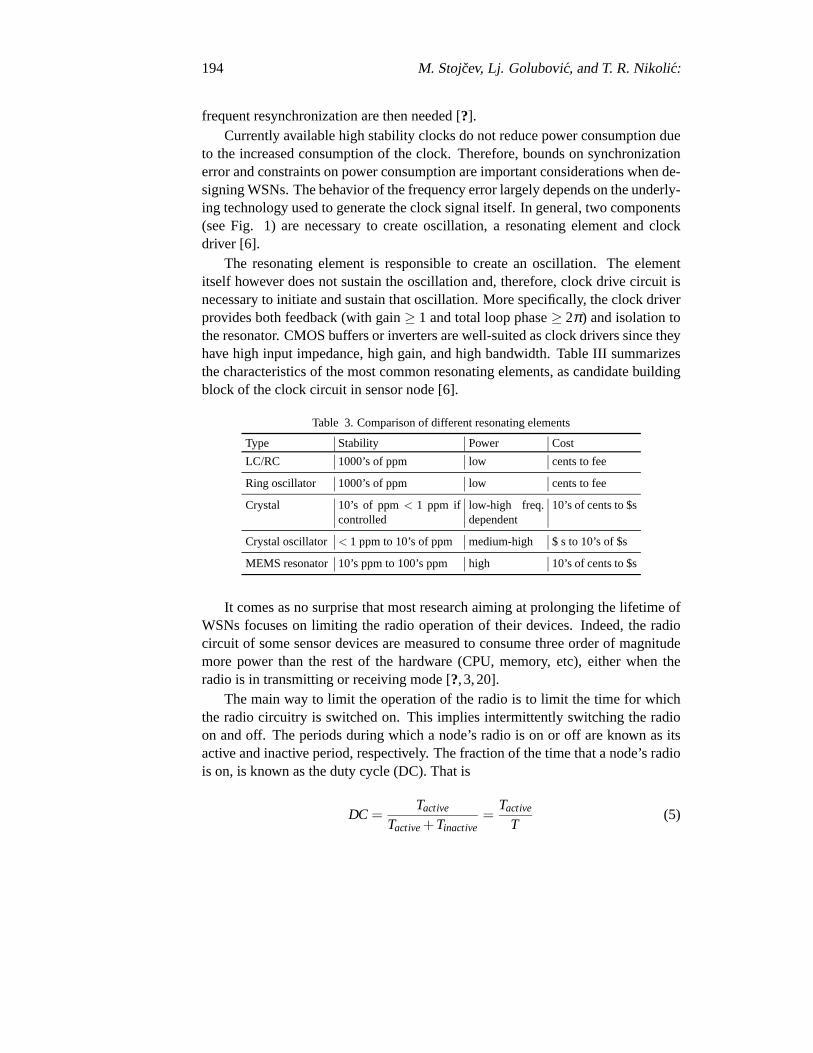
The resonating element is responsible to create an oscillation. The elementitself however does not sustain the oscillation and, therefore, clock drive circuit isnecessary to initiate and sustain that oscillation. More specifically, the clock driverprovides both feedback (with gain≥ 1 and total loop phase≥ 2π) and isolation tothe resonator. CMOS buffers or inverters are well-suited as clock drivers since theyhave high input impedance, high gain, and high bandwidth. Table III summarizesthe characteristics of the most common resonating elements, as candidate buildingblock of the clock circuit in sensor node [6].

Table 3. Comparison of different resonating elements

Type Stability Power Cost

LC/RC 1000’s of ppm low cents to fee

Ring oscillator 1000’s of ppm low cents to fee

Crystal 10’s of ppm< 1 ppm ifcontrolled

low-high freq.dependent

10’s of cents to $s

Crystal oscillator < 1 ppm to 10’s of ppm medium-high $ s to 10’s of $s

MEMS resonator 10’s ppm to 100’s ppm high 10’s of cents to $s

It comes as no surprise that most research aiming at prolonging the lifetime ofWSNs focuses on limiting the radio operation of their devices. Indeed, the radiocircuit of some sensor devices are measured to consume three order of magnitudemore power than the rest of the hardware (CPU, memory, etc), either whentheradio is in transmitting or receiving mode [?, 3,20].

The main way to limit the operation of the radio is to limit the time for whichthe radio circuitry is switched on. This implies intermittently switching the radioon and off. The periods during which a node’s radio is on or off are known as itsactive and inactive period, respectively. The fraction of the time that a node’s radiois on, is known as the duty cycle (DC). That is

DC =Tactive

Tactive+Tinactive=

Tactive

T(5)


For example, a node that is active for 10 ms every second has a duty cycleof

DC =10ms

1000ms= 1%

The duty cycled-based operation of the nodes makes the synchronizationof theactive periods of their frames essential. Nodes whose active periods donot overlapcannot communicate with each other. In this paper we focus on the problem howfor a given clock oscillator, and as small as possible duty cycle, to providecorrectsynchronization of the sensor node within the WSN.

10 Low Power MCU for SN

The battery-powered SNs ( developed as small intelligent devices in homes,planta-tions, oceans, rivers, streets, and highways to monitor the real-world environment)in which the battery must lost for up to ten years (frequent battery replacementis undesirable) are applications for which power consumption is very important.As these devices become increasingly power-conscious, the need for smart powermanagement becomes equally significant and demand for usage of ultralow powermicrocontroller unit (MCU), as SN’s constituent, is rising. The choice of MCUis critical, too. In a attempt to prolong battery life, software engineers go to greatlengths to optimize code, minimize memory accesses, etc. Hardware engineers fo-cus on ways to shut down unused circuitry, ensure that all quiscent currents andleakage paths are minimized, and maximize power-supply efficiency [21].

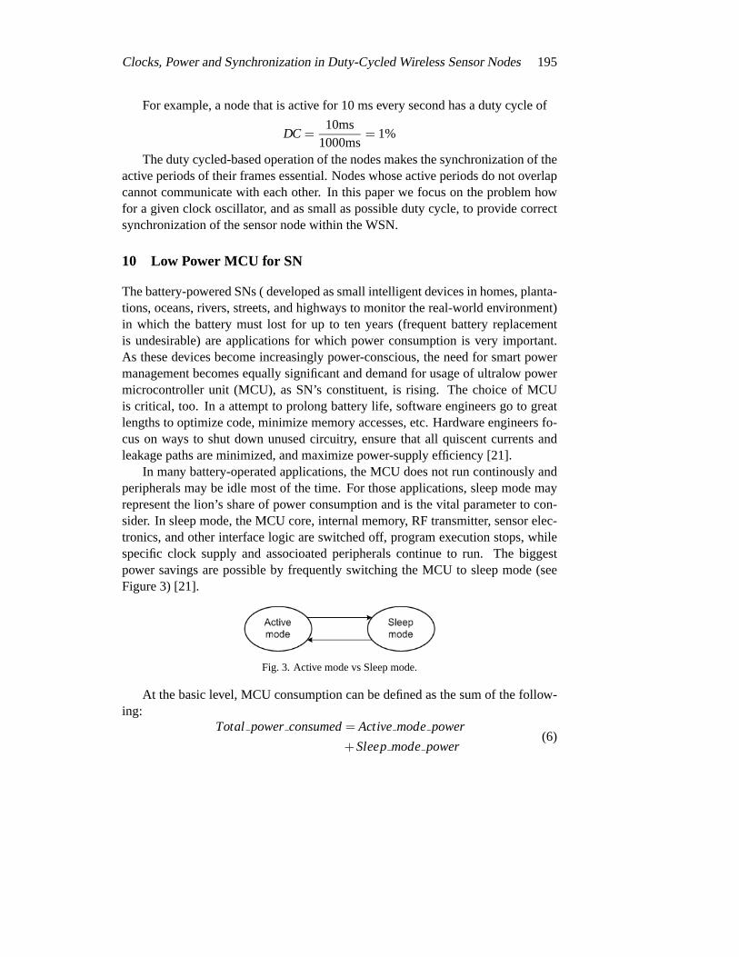
In many battery-operated applications, the MCU does not run continously andperipherals may be idle most of the time. For those applications, sleep mode mayrepresent the lion’s share of power consumption and is the vital parameterto con-sider. In sleep mode, the MCU core, internal memory, RF transmitter, sensorelec-tronics, and other interface logic are switched off, program execution stops, whilespecific clock supply and associoated peripherals continue to run. The biggestpower savings are possible by frequently switching the MCU to sleep mode (seeFigure 3) [21].

Fig. 3. Active mode vs Sleep mode.

At the basic level, MCU consumption can be defined as the sum of the follow-ing:

Total power consumed= Activemodepower

+Sleepmodepower(6)


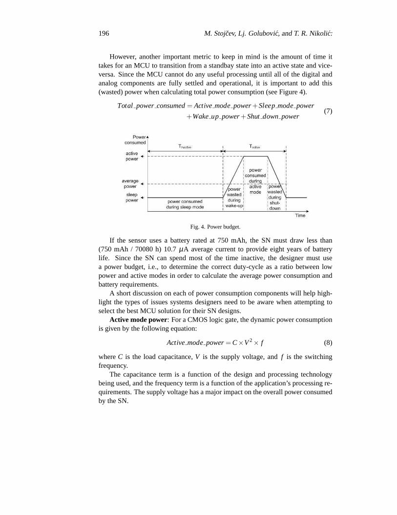
However, another important metric to keep in mind is the amount of time ittakes for an MCU to transition from a standbay state into an active state and vice-versa. Since the MCU cannot do any useful processing until all of the digital andanalog components are fully settled and operational, it is important to add this(wasted) power when calculating total power consumption (see Figure 4).

Total power consumed= Activemodepower+Sleepmodepower

+Wakeup power+Shut down power(7)

Fig. 4. Power budget.

If the sensor uses a battery rated at 750 mAh, the SN must draw less than(750 mAh / 70080 h) 10.7µA average current to provide eight years of batterylife. Since the SN can spend most of the time inactive, the designer must usea power budget, i.e., to determine the correct duty-cycle as a ratio between lowpower and active modes in order to calculate the average power consumption andbattery requirements.

A short discussion on each of power consumption components will help high-light the types of issues systems designers need to be aware when attempting toselect the best MCU solution for their SN designs.

Active mode power: For a CMOS logic gate, the dynamic power consumptionis given by the following equation:

Activemodepower= C×V2× f (8)

whereC is the load capacitance,V is the supply voltage, andf is the switchingfrequency.

The capacitance term is a function of the design and processing technologybeing used, and the frequency term is a function of the application’s processing re-quirements. The supply voltage has a major impact on the overall power consumedby the SN.


Advanced power architecture, such as on-chip low drop-out linear voltage regu-lator, voltage islands, dynamic threshold voltage control, etc., can be used tomain-tain a constant active current over the full operating voltage range andcan helpsystems designer to achieve a significant savings in power consumption [22].

Sleep mode power: To save energy in WSN it is a desirable to keep SNs inlow-power state, if not turned off completely, for as long as possible. SN hardwareis often designed with this goal in mind; processor have various “sleep” modes oris capable of powering down high-energy peripherals when not in use.

Running the MCU at full-speed all the time will never lead to a truly low-power design even if the lowest-power MCU is used. The biggest power savingsare only possible by frequently switching the MCU to a low power sleep statefrom normal state and vice-versa. The MCU is switched into low-power modebyconfiguring bits in the status and control registers, i.e. by issuing a sleep commandover the bus. Achieving maximum energy efficiency (and battery life) translatesinto ensuring that each MCU task consumes the minimum possible current at theminimum possible voltage for the shortest possible duration, so that the devicespends the majority of its time in very low-power sleep mode. The sleep, or lowpower mode, vary in degree to which the MCU is aware of its surroundings andthe different clocks that the SN must keep runing. The more common sleep modesare Idle mode, Power Save, and Power Down [23]. Idle mode is a shallow sleepmode where only parts of the SN are shut down but the main parts of the MCUare running. In Power Save mode, everything is turned off except a 32kHz clockrunning from a crystal to keep track of the time. It allows only the base timer orwatch prescaler to work. The operating clock for the MCU and peripheral resourcesis stopped in this mode to reduce the power consumption. In Power Down mode,everything is is shut down, including the clock source. All clocks are halted, butthe MCU status, RAM and register contents are preserved. It has the lowest currentconsumption and only external interrupts can wakeup MCU from Power Downmode [23].

The advantage of having multiple sleep modes is the flexibility it provides toshut down any part of the SN that is not absolutely necessary to the function athand. The amount of power that can be saved depends on the mode beingused.

Most vendors offer different standby low-power option. Most suppliers willhighlight their absolute lowest sleep mode current, which will often correspond tothe current being consumed with the real-time clock and brownout detector (contin-uous supply voltage monitoring) disabled. Some vendors will go a step further andquote a shutdown mode current that does not retain memory and requires aresetto wake up, which in general is not a very practical mode [3, 23]. Therefore, sincemost applications will require full RAM and register retention, it is important fora system designer to perform a side-by-side comparisons based on the following


metrics [23]:

1. Sleep mode current with real-time clock and brownout disabled (with RAMretention),

2. Sleep mode current with real-time clock disabled and brownout enabled,

3. Sleep mode current with real-time clock and brownout enabled.

A system designer can then use the corect values when calculating the overallsleep mode power budget based on the duty cycle of their application.

Wake-up and shut-down power mode: In systems that use sleep mode a sig-nificant amount of power can be wasted waking up (shut-down) the SN and prepar-ing it to acquire or process data. In fact, in certain applications an SN can often usejust as much energy when comming out of sleep (standby) as when the SN is fullyprocessing data. Therefore, it is important to design an SN to wake-up (shut-down)and settle in an extremelly short amount of time in order to minimize the amountof time spent in an energy-wasting state.

The SN, ie. the MCU, should be able to exit sleep mode from either an externaltrigger or an interval timer. The most flexible periodic wake-up (shut-down) sourceis a real-time clock having the capability of being run from an external crystaloscillator or from a low-frequency internal ring oscillator that eliminates the needfor a crystal in lower-accuracy applications, like that used in agriculture. Avoidusing a slow-starting crystal oscillator for high-speed clock; an accurate, quick-starting, on-chip oscillator is a better alternative.

Something as conclusion concernig selection of low-power MCU: Having inmind that every SN application will be affected by the combination of sleep modepower, active mode power and wake-up and shut-down mode power, it may be help-ful for systems designers to simply start any analysis by sistematically breakingdown the power consumption numbers into the parts afore mentioned. Once thesenumbers have been derived, a system designer can then factor in the application’sduty cycles - the amont of time the application expects to spend in sleep, active,wake-up and shut-down modes - to calculate an overall average consumption num-ber. The resulting value should provide the system designer a close approximationthat can be used to objectively evaluate and compare SN alternatives to achieve thelowest possible system-level power consumption.

The primary factor of low-power modes is that recovering (wake-up) intonor-mal operating modes and returning to low power mode can impose a significantdelay. Therefore, a key feature to look in any MCU is the shortest wake-up andshut-down time. MCU wake-up time from some low-power modes should be fastenough to meet the response times of interrupts. TotalTrestoreis approximatyely 3.5ms withTwake−up =1.4 ms,Tshut−down= 1 ms with PLL stabilization of 1 ms, and


gear-up time of about 75µs. This illustrates the ability to optimize the design forlow-power while having a flexible architecture in the MCU that helps to achievehigh-performance and low-power consumption.

11 Battery Issues

From the system’s perspective, a good micro-battery should have the followingfeatures [21]: 1) high energy density; 2) large active volume to packaging volumeratio; 3) small cell potential (0.5 - 1.0 V) so digital circuits can take advantages ofthe quadratic reduction in power consumption with supply voltage; 4) efficientlyconfigured into series batteries to provide a variety of cell potentials for variouscomponents of the system without requiring the overhead of voltage converters; 5)rechargeable in case the system has an energy harvester.

A number of small batteries are being developed until now for wireless commu-nications. It seems that three cell chemistries currently dominate the growing wire-less sensor network application market: Nickel-Metal Hydride (NiMH), LithiumIon (Li-Ion), and Lithium Polymer (Li-polymer).

Each battery type has unique characteristics that make it appropriate, or in-appropriate, for a SN. Knowing the specific characteristics of each cellchemistryin terms of voltage, cycles, load current, energy density, charge time, anddischargerates is the first step in selecting a cell for a SN. The following discussion gives ashort overview of the characteristics, strengths, and weaknesses ofeach of the threecell chemistries.

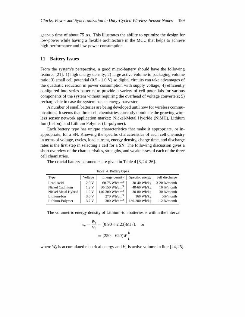
The crucial battery parameters are given in Table 4 [3,24–26].

Table 4. Battery types

Type Voltage Energy density Specific energy Self discharge

Lead-Acid 2.0 V 60-75 Wh/dm3 30-40 Wh/kg 3-20 %/monthNickel Cadmium 1.2 V 50-150 Wh/dm3 40-60 Wh/kg 10 %/monthNickel Metal Hybrid 1.2 V 140-300 Wh/dm3 30-80 Wh/kg 30 %/monthLithium-Ion 3.6 V 270 Wh/dm3 160 Wh/kg 5%/monthLithium-Polymer 3.7 V 300 Wh/dm3 130-200 Wh/kg 1-2 %/month

The volumetric energy density of Lithium-ion batteries is within the interval

we =We

V1= (0.90÷2.23)MJ/L or

= (250÷620)WhL

whereWe is accumulated electrical energy andV1 is active volume in liter [24,25].


If we assume thatwe = 2 MJ/L, the useful volumeV1 = 103 L and the nominalbattery operating voltage (average potential difference) isEB = 3.6 V then we have

1. The accumulated electrical energy into a form of chemical energy is

Wch = weV1 = 2×106×103 = 2×10−3 J

2. The electrical energy which, from battery with nominal operating voltageEB = 3.6 V during the battery life-timetB, is delivered in a form of work, foran average current ofIa = 8 µA, is equal to

Ee = EbIatB = 3.6×8×10−6× tB

ForWCh = We it is possible to determine the usage battery time

tB =2×103

3.6×8×10−6 = 69 444 444 s

Since in one year we have 365×24×3 600= 31 536 000 s, by dividing withthis value we obtain

tB =69 444 44431 536 000

= 2.202 years

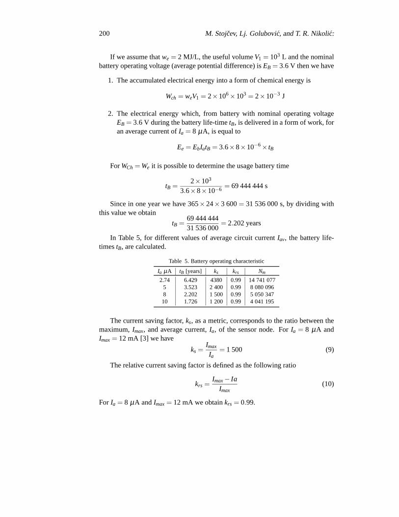
In Table 5, for different values of average circuit currentIav, the battery life-timestB, are calculated.

Table 5. Battery operating characteristic

Ia µA tB [years] ks krs Nm

2.74 6.429 4380 0.99 14 741 0775 3.523 2 400 0.99 8 080 0968 2.202 1 500 0.99 5 050 34710 1.726 1 200 0.99 4 041 195

The current saving factor,ks, as a metric, corresponds to the ratio between themaximum,Imax, and average current,Ia, of the sensor node. ForIa = 8 µA andImax= 12 mA [3] we have

ks =Imax

Ia= 1 500 (9)

The relative current saving factor is defined as the following ratio

krs =Imax− Ia

Imax(10)

For Ia = 8 µA andImax= 12 mA we obtainkrs = 0.99.


The total number of measuring cycles forDC = 10−3, Nm, is given by

Nm =tB

tcycle(11)

For Ia = 8 µA, tcycle= 13.75 s, number of transmitted bytes per packet 64, and datatransfer rate 50 kbps, we haveNm = 14 741 077.

In Table 5 calculated values forks, krs andNm, for different average currentIa,and fixedDC andtcycle are given.

12 Workload Profile of Sensor Node

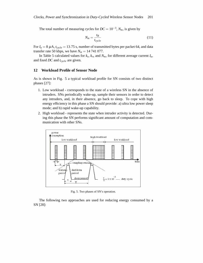
As is shown in Fig. 5 a typical workload profile for SN consists of two distinctphases [27]:

1. Low workload - corresponds to the state of a wireless SN in the absenceofintruders. SNs periodically wake-up, sample their sensors in order to detectany intruders, and, in their absence, go back to sleep. To cope with highenergy efficiency in this phase a SN should provide: a) ultra low power sleepmode; and b) rapid wake-up capability.

2. High workload - represents the state when intruder activity is detected. Dur-ing this phase the SN performs significant amount of computation and com-munication with other SNs.

Fig. 5. Two phases of SN’s operation.

The following two approaches are used for reducing energy consumedby aSN [28]:


1. duty cycling - consists of waking-up the SN only for the time needed to ac-quire a new set of samples and then powering it off immediately afterwards;

2. adaptive-sensing strategy - is able to dynamically change the SN activity tothe real dynamics of the process.

Power consumption is the product of operating voltage,EB = VCC, multipliedby the current consumption,ICC. UsuallyICC is the only measure while describingpower characteristics of a SN or the chip. This is a mistake because decreasingVCC

directly reduces the current consumption and the overall power gain. Inlow powerdesigns, the average current consumption,Ia, determines battery life.

13 Implementation of Duty Cycle Technique

As we have already mentioned radio duty-cycling has received significant atten-tion in sensor networking, particularly in the form of MAC protocols and topologymanagement.

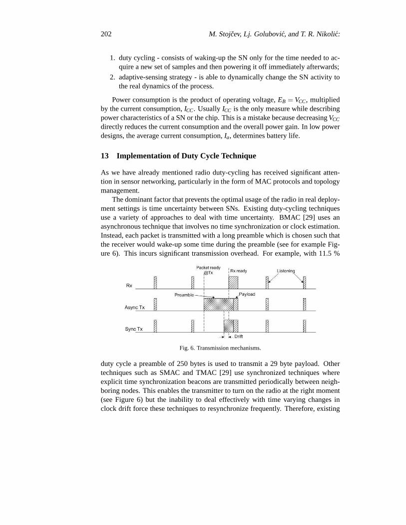
The dominant factor that prevents the optimal usage of the radio in real deploy-ment settings is time uncertainty between SNs. Existing duty-cycling techniquesuse a variety of approaches to deal with time uncertainty. BMAC [29] uses anasynchronous technique that involves no time synchronization or clock estimation.Instead, each packet is transmitted with a long preamble which is chosen suchthatthe receiver would wake-up some time during the preamble (see for example Fig-ure 6). This incurs significant transmission overhead. For example, with 11.5 %

Fig. 6. Transmission mechanisms.

duty cycle a preamble of 250 bytes is used to transmit a 29 byte payload. Othertechniques such as SMAC and TMAC [29] use synchronized techniqueswhereexplicit time synchronization beacons are transmitted periodically between neigh-boring nodes. This enables the transmitter to turn on the radio at the right moment(see Figure 6) but the inability to deal effectively with time varying changes inclock drift force these techniques to resynchronize frequently. Therefore, existing


radio duty-cycling approaches expend a lot of energy in handling time uncertaintybetween SNs.

Typical frequency skew of±30-50 ppm due to manufacturing variations, andadditional±10-20 ppm due to temperature variation, and an exponentially decreas-ing ±3 ppm per year are common [30]. These frequencies skews result in relativeclock disproportion between SNs, and, as a result, SNs must include a guard time,equal to the maximum drift, which grows linearly with the interval between com-munications [6, 30]. Letsskew(∆ f/ f in Hz/Hz) be the frequency skew andTtot bethe total packet period, than the minimum guard time becomes

tguard = 2sskewTtot (12)

If it takes tsp time to send a packet, then the total transmission time will betguard+ tsp and theDC is

DC =2sskewTtot + tsp

Ttot(13)

which can be simplified to

DC = 2sskew+tsp

Ttot(14)

Equation (14) establishes a lower bound of 2sskew on theDC and points tothree solutions how to reduce radio on-time [30]. The first solution is basedon re-ducing the frequency skew with higher tolerance crystal oscillators, power-hungrytemperature-compensated crystal oscillators, or improved calibration. A secondsolution is to reduce the packet transmission time by increasing the radio speed.Reducing radio wake-up and shut-down times is also preferable. The thirdsolutiondeals with decreasing the data rate by increasing the communications period.

Most of the proposed techniques for time synchronization ignore the poweroverhead that a time synchronization protocol introduces. In general ifa systemneeds less than 10 ms accuracy, then a time synchronization of up to 1000 s issuf-ficient to guarantee such approaches. In most systems, this interval is much largerthan the communication interval necessary to transmit sensor data from the nodesto a fusion center and we can assume that the overhead of time synchronizationin these scenarios is minimal. However, if high accuracy is needed the synchro-nization intervals have to be of the order of tens of seconds. In these cases, timesynchronization could be piggy-backed on regular messages, only introducing asmall message overhead of the order of a timestamp.

As we have already mentioned each within WSN has its own clock oscilla-tor. From metrological point of view the relative measuring inaccuracies,C, of theoscillator is in order of

δr =∆ttw

∼ 10−5 (15)


where∆t corresponds to absolute measuring inaccuracy during the observed timeinterval of durationtw.

According to eq (15) it is possible now to form the following two equations:

tw = k1t (16)

and

tw =k2

δr(t)(17)

By adding equations (16) and (17) and dividing by two we obtain

tw =12

[

k1∆t +k2

δr(t)

]

(18)

From the condition dtw/d(∆t) = 0 we determine the constantk2

k2 = ∆t (19)

Having in mind that the left sides of eqs (13) and (14) are identical, and bysubstituting the result derived in eq. (16) we obtain

k1 =1

δr(t)(20)

By substituting the results obtained in eqs (19) and (20) into (16) we obtain

tw = k1k2 =∆t

δr(t)(21)

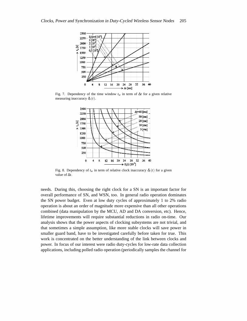
According to eq. (16) we can conclude that the minimal width of the timewindow t increases as the error of clock reading∆t increases (refer to Figure 7).

In a similar way, equation (17) points out to the relative clock error decreasing,as thetw width increases (refer to Figure 8).

As a conclusion we can say that: the minimal width of a time windowtw de-pends of the relative oscillator errorδr(t) for a given value∆t.

14 Conclusion

Clock synchronization is a critical component in the operation of WSNs as it pro-vide common frame to different nodes. WSNs make heavy use of synchronizedtime, but often have unique requirements in respect to lifetime of SN, precisionof synchronization achieved, as well as the time and energy required to achieveit. Existing time synchronization methods need to be extended to meet all these


Fig. 7. Dependency of the time windowtw in term of ∆t for a given relativemeasuring inaccuracyδr (t).

Fig. 8. Dependency oftw in term of relative clock inaccuracyδr (t) for a givenvalue of∆t.

needs. During this, choosing the right clock for a SN is an important factorforoverall performance of SN, and WSN, too. In general radio operationdominatesthe SN power budget. Even at low duty cycles of approximately 1 to 2% radiooperation is about an order of magnitude more expensive than all other operationscombined (data manipulation by the MCU, AD and DA conversion, etc). Hence,lifetime improvements will require substantial reductions in radio on-time. Ouranalysis shows that the power aspects of clocking subsystems are not trivial, andthat sometimes a simple assumption, like more stable clocks will save power insmaller guard band, have to be investigated carefully before taken for true. Thiswork is concentrated on the better understanding of the link between clocksandpower. In focus of our interest were radio duty-cycles for low-rate data collectionapplications, including polled radio operation (periodically samples the channel for


radio activity and power-down the radio between successive samples) and sched-uled radio-operation (establishes well-known and periodic time intervals when it islegal (or illegal) to transmit). Our proposal is to use piggy-backing as the processof combining the data fusion messages with messages that carry synchronizationdata among nodes. Instead of sending independent clock synchronization mes-sages, these messages are piggy-backed on the data fusion messages that have tobe send to the SN. Piggy-backing is clearly advantageous because WSNsare oftensubject to limited communication bandwidth and power-consumption constraints.Further research has to be done on the link between clock stability and its effecton time synchronization. Currently, 1µs seems to be the lower and of what ispossible for time synchronization in WSN with current technology [31]. Futureresearch will show why this is the case, and where the bottlenecks are, in order tobreak this barrier. The challenge will definitely lay in providing such accuracieswhile still maintaining the low-power requirements given by the power constraintsof WSNs [31].

Acknowledgement

This work was supported by the Serbian Ministry of Science and TechnologicalDevelopment, Project No. TR-32009 - “Low-Power Reconfigurable Fault-TolerantPlatforms”.

References

[1] S. Soloman,Sensors and Control Systems in Manufacturing. New York: McGrawHill, 2010.

[2] A. Hac,Wireless Sensor Network Designs. Chichester: John Wiley & Sons, 2003.

[3] M. Stojcev, M. Kosanovic, and L. Goluibovic, “Power management and energy har-vesting techniques for wireless sensor nodes,” inProc. of IX International Conferenceon Telecommunications in Modern Satellite, Cable and Broadcasting Services, vol. 1,Nis, Serbia, Oct. 7–9, 2009, pp. 65–72.

[4] E. Serpedin and Q. M. Chaudhari,Synchronization in WSN: Parameter Estimation,Performance Benchmarks and Protocols. Cambridge University Press, 2009.

[5] Q. Yik-Chung Wu Chaudhari and E. Serpedin, “Clock synchronization of wirelesssensor networks,”IEEE Signal Processing Magazine, vol. 28, no. 1, pp. 124–138,Jan. 2011.

[6] T. Schmid, R. Shea, Z. Charbiwala, J. Freidman, and M. B. Srivastava, “On the inter-action of clocks, power, and synchronization in duty-cycled embedded sensor nodes,”ACM Transactions on Sensor Networks, vol. 7, no. 3, pp. 24.1–24.19, Sept. 2010.

[7] B. Sundararaman, U. Buy, and A. D. Kshemkalyani, “Clock synchronization forwireless sensor networks: A survey,”Ad Hoc Networks, vol. 3, no. 3, pp. 281–323,2006.

[8] J. Syh and M. Horton, “Powering sensor networks,”IEEE Potentials, vol. 23, no. 3,pp. 35–38, Nov. 2004.


[9] M. Maroti, B. Kusy, G. Simon, and A. Ledeczi, “The floodingtime synchronizationprotocol,” in Proc. of the 2nd International Conference on Embedded NetworkedSensor Systems, SynSys’04, Baltimor, Maryland, USA, Nov. 3–5, 2004, pp. 39–49.

[10] A. Ageev, “Time synchronization and energy efficiency in wireless sensor networks,”Ph.D. dissertation, DISI - University of Trento, Mar. 2010.

[11] K. Romer, “Time synchronization in ad hoc networks,” inProceedings of the Inter-national Symposium on Mobile Ad Hoc Networking and Computing (MobiHoc 01),Long Beach, CA, USA, Oct. 2001, pp. 173–182.

[12] J. Elson, L. Girod, and D. Estrin, “Fine-grained network time synchronization usingreference broadcasts,” inProc. Symposium on Operating Systems Design and Imple-mentation (OSDI), vol. 36, Boston, MA, USA, Dec. 2002, pp. 147–163.

[13] S. Ganeriwal, R. Kumar, and M. B. Srivastava, “Timing-sync protocol for sensor net-works,” in Proc. International Conference on Embedded Networked Sensor Systems(SenSys), Los Angeles, CA, USA, Nov. 2003, pp. 138–149.

[14] M. L. Sichitiu and C. Veerarittiphan, “Simple, accurate time synchronization forwireless sensor networks,” inProc. Wireless Communi-cations and Networking Con-ference (WCNC 2003), vol. 2, 2003, pp. 1266–1273.

[15] J. van Greunen and J. Rabaey, “Lightweight time synchronization for sensor net-works,” in Proc. ACM International Conference on Wireless Sensor Networks andApplications (WSNA), San Diego, CA, USA, Sept. 2003, pp. 11–19.

[16] S. Palchaudhuri, A. K. Saha, and D. B. Johnson, “Adaptive clock synchronizationin sensor networks,” inProc. International Symposium on Information Processing inSensor Networks (IPSN), Apr. 2004, pp. 340–348.

[17] K. Shahzad, A. Ali, and N. D. Gohar, “ETSP: An energy-efficient time synchroniza-tion protocol for wireless sensor networks,” inProc. International Conference onAdvanced Information Networking and Applications (AINAW), Mar. 2008, pp. 971–976.

[18] S. Ganeriwal, D. Ganesan, H. Shim, V. Tsiatsis, and M. B.Srivastava, “Estimatingclock uncertainty for efficient duty-cycling in sensor networks,” in Proc. Interna-tional Conference on Embedded Networked Sensor Systems (SenSys), San Diego,CA, USA, Nov. 2005, pp. 130–141.

[19] F. Sivrikaya and B. Yener, “Time synchronization in sensor networks: a survey,”IEEE Network, vol. 18, no. 4, pp. 45–50, 2004.

[20] V. Raghunathan, C. Schurgers, S. Park, and M. Srivastan, “Energy aware wirelessmicrosensor networks, IEEE Signal Processing Magazine,” vol. 19, no. 3, pp. 40–50,Mar. 2002.

[21] J. E. Elson, “Time synchronization in WSN,” Ph.D. dissertation, University of Cali-fornia, Los Angeles, 2003.

[22] M. Salas. (2011, May) Low power design basics: How to choose the optimallow power MCU for your embedded system. [Online]. Available: http://low-powerdesign.com/PDF/Low-Power-Design-Basics.pdf

[23] R. Dasgupta. (2011, May) Low power MCU selection criteria and sleepmode implementation using hardware/software codesign technique. [Online].Available: http://www.eetimes.com /design/industrial-control/4014277/Low-power-MCU-selection-criteria-and-sleep-mode-implementation

[24] F. Pistoia,Battery operated devices and systems: From portable electronics to indus-trial products. Amsterdam: Elsevier, 2008.

[25] (2011, May) Lithium-ion battery. [Online]. Available: http://en.wikipedia.org/wiki/Lithium-ion battery#citenote-greencarcongress-1


[26] E. Jens, “Low-power design methodologies for embeddedinternet systems,” Ph.D.dissertation, EISLAB, Lulea University of Technology, Sweden, 2008.

[27] V. Raghunathan, S. Ganeriwal, and M. Srivastava, “Emerging techniques for longlived wireless sensor networks,”IEEE Communication Magazine, vol. 44, no. 4, pp.108–114, Apr. 2006.

[28] C. Alippi, G. Anastasi, M. Di Francesco, and M. Roveri, “Energy management inwireless sensor networks with energy-hugry sensors,”IEEE Instrumentation & Mea-surement Magazine, vol. 12, no. 2, pp. 16–23, Apr. 2009.

[29] S. Ganeriwal, D. Ganesan, H. Sim, V. Tsiatsis, and M. B. Srivastava. (2011,May) Estimating clock uncertainty for efficient duty-cycling in sensor networks.[Online]. Available: http://nesl.ee.ucla.edu/fw/documents/journal/2008/Ganeriwal08 TNET.pdf

[30] P. Dutta, D. Culler, and S. Shenker. (2011, May 20,) Procrastination might leadto a longer and more useful life. [Online]. Available: http://iteseerx.ist.psu.edu/viewdoc/download?doi=10.1.1.93

[31] T. Schmid, R. Shea, J. Friedman, Z. Charbiwala, M. B. Srivastava, and Y. H. Cho.(2011, May) On the interaction of clocks and power in embedded sensor nodes.[Online]. Available: http://nesl.ee.ucla.edu/fw/thomas/schmid2009techreport.pdf

Clocks, Power and Synchronization in Duty-Cycled Wireless

Documents

Transcript of Clocks, Power and Synchronization in Duty-Cycled Wireless