Climate Change: Climate Change:

Moonshine, Millions of Models, & Billions of DataMoonshine, Millions of Models, & Billions of Data

New Ways to Sort Fact from FictionNew Ways to Sort Fact from Fiction

Bruce WielickiBruce Wielicki

March 21, 2007March 21, 2007

University of Miami LectureUniversity of Miami Lecture

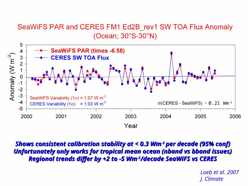
Shows consistent calibration stability at < 0.3 WmShows consistent calibration stability at < 0.3 Wm-2 -2 per decade (95% conf)per decade (95% conf)Unfortunately only works for tropical mean ocean (nband vs bband issues)Unfortunately only works for tropical mean ocean (nband vs bband issues)

Regional trends differ by +2 to -5 WmRegional trends differ by +2 to -5 Wm-2-2/decade SeaWiFS vs CERES/decade SeaWiFS vs CERES

Loeb et al. 2007J. Climate

0.21 Wm-2

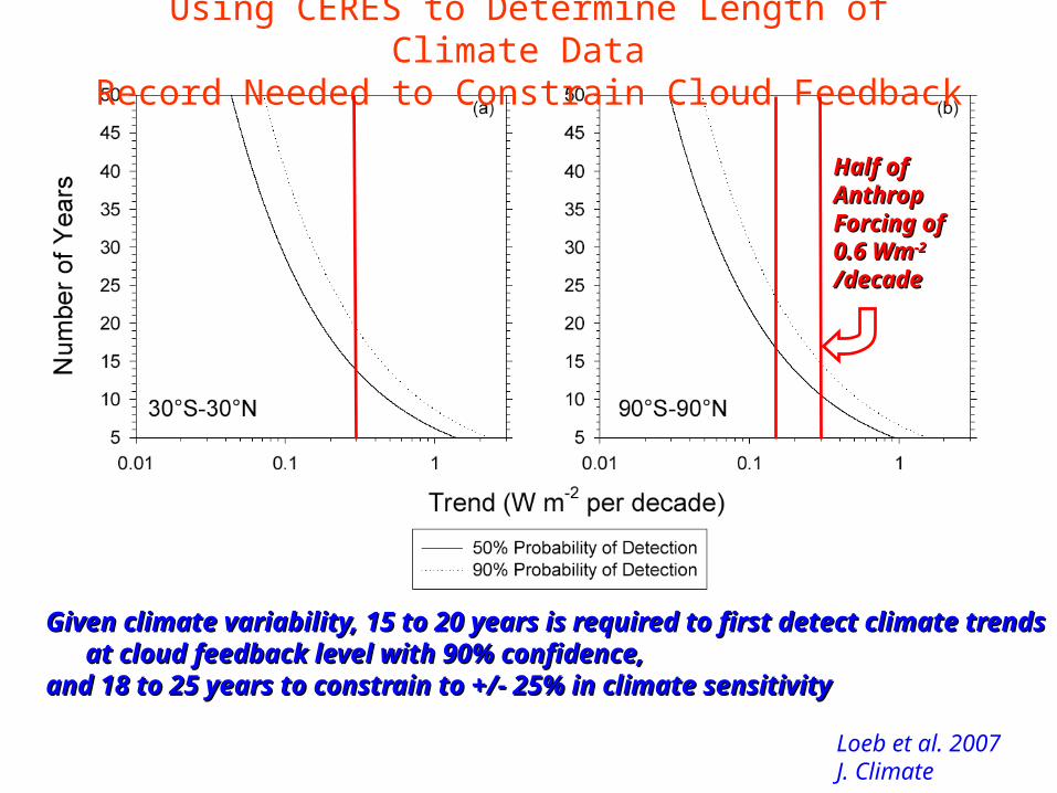
Using CERES to Determine Length of Climate Data Record Needed to Constrain Cloud Feedback

Given climate variability, 15 to 20 years is required to first detect climate trends Given climate variability, 15 to 20 years is required to first detect climate trends at cloud feedback level with 90% confidence,at cloud feedback level with 90% confidence,

and 18 to 25 years to constrain to +/- 25% in climate sensitivityand 18 to 25 years to constrain to +/- 25% in climate sensitivity

Half ofHalf ofAnthropAnthropForcing of Forcing of 0.6 Wm0.6 Wm-2-2

/decade/decade

Loeb et al. 2007J. Climate

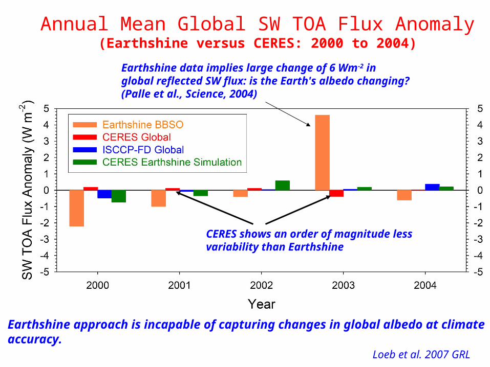
Annual Mean Global SW TOA Flux Anomaly(Earthshine versus CERES: 2000 to 2004)

Loeb et al. 2007 GRL

Earthshine data implies large change of 6 Wm-2 inglobal reflected SW flux: is the Earth's albedo changing? (Palle et al., Science, 2004)

CERES shows an order of magnitude lessvariability than Earthshine

Earthshine approach is incapable of capturing changes in global albedo at climate accuracy.

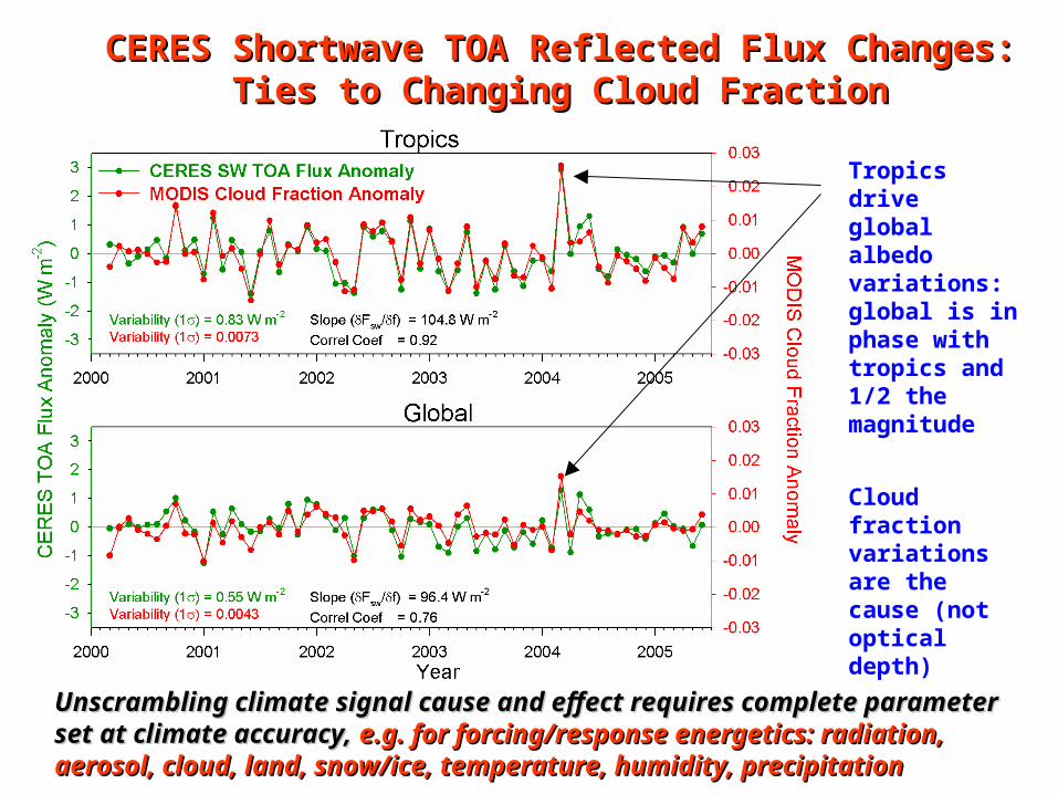
CERES Shortwave TOA Reflected Flux Changes: CERES Shortwave TOA Reflected Flux Changes: Ties to Changing Cloud FractionTies to Changing Cloud Fraction

Unscrambling climate signal cause and effect requires complete parameter Unscrambling climate signal cause and effect requires complete parameter set at climate accuracy, set at climate accuracy, e.g. for forcing/response energetics: radiation, e.g. for forcing/response energetics: radiation, aerosol, cloud, land, snow/ice, temperature, humidity, precipitationaerosol, cloud, land, snow/ice, temperature, humidity, precipitation

Tropics drive global albedo variations:global is in phase with tropics and 1/2 the magnitude

Cloud fractionvariations are the cause (not optical depth)

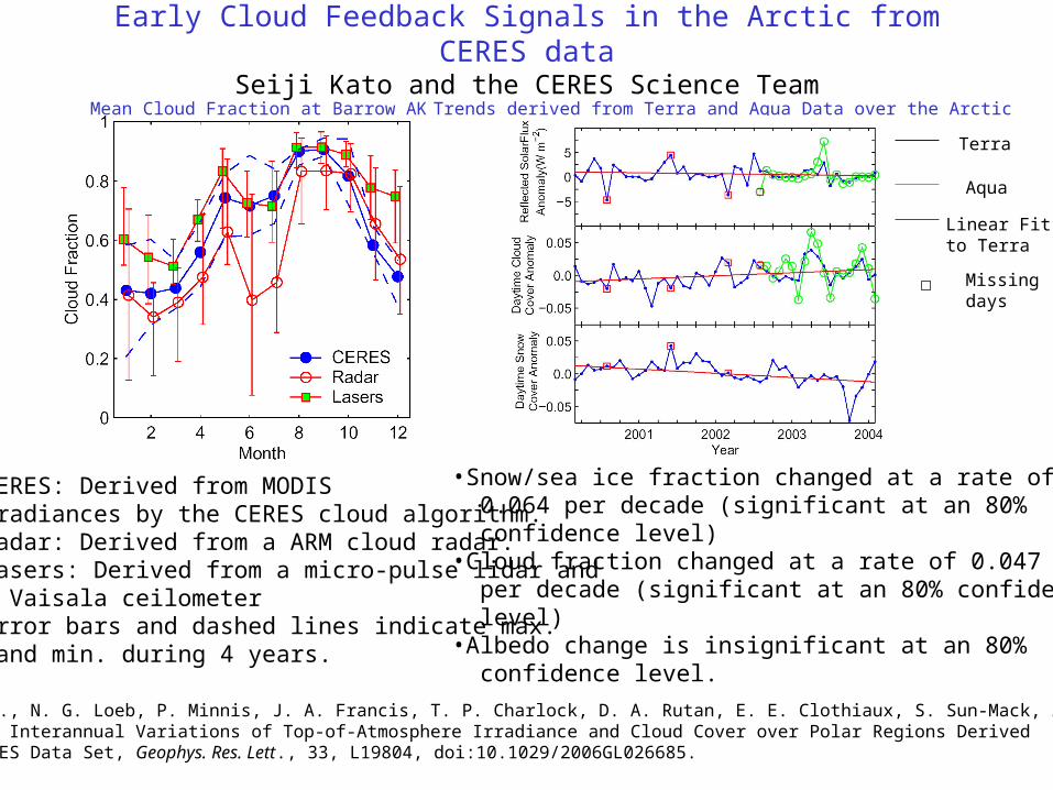
Early Cloud Feedback Signals in the Arctic from CERES dataSeiji Kato and the CERES Science Team

•CERES: Derived from MODIS radiances by the CERES cloud algorithm.•Radar: Derived from a ARM cloud radar.•Lasers: Derived from a micro-pulse lidar and a Vaisala ceilometer•Error bars and dashed lines indicate max. and min. during 4 years.

•Snow/sea ice fraction changed at a rate of 0.064 per decade (significant at an 80% confidence level)•Cloud fraction changed at a rate of 0.047 per decade (significant at an 80% confidence level) •Albedo change is insignificant at an 80% confidence level.

From Kato, S., N. G. Loeb, P. Minnis, J. A. Francis, T. P. Charlock, D. A. Rutan, E. E. Clothiaux, S. Sun-Mack, 2006:Seasonal and Interannual Variations of Top-of-Atmosphere Irradiance and Cloud Cover over Polar Regions Derived from the CERES Data Set, Geophys. Res. Lett., 33, L19804, doi:10.1029/2006GL026685.

Mean Cloud Fraction at Barrow AK Trends derived from Terra and Aqua Data over the Arctic

Terra

Aqua

Linear Fit to Terra

Missing days

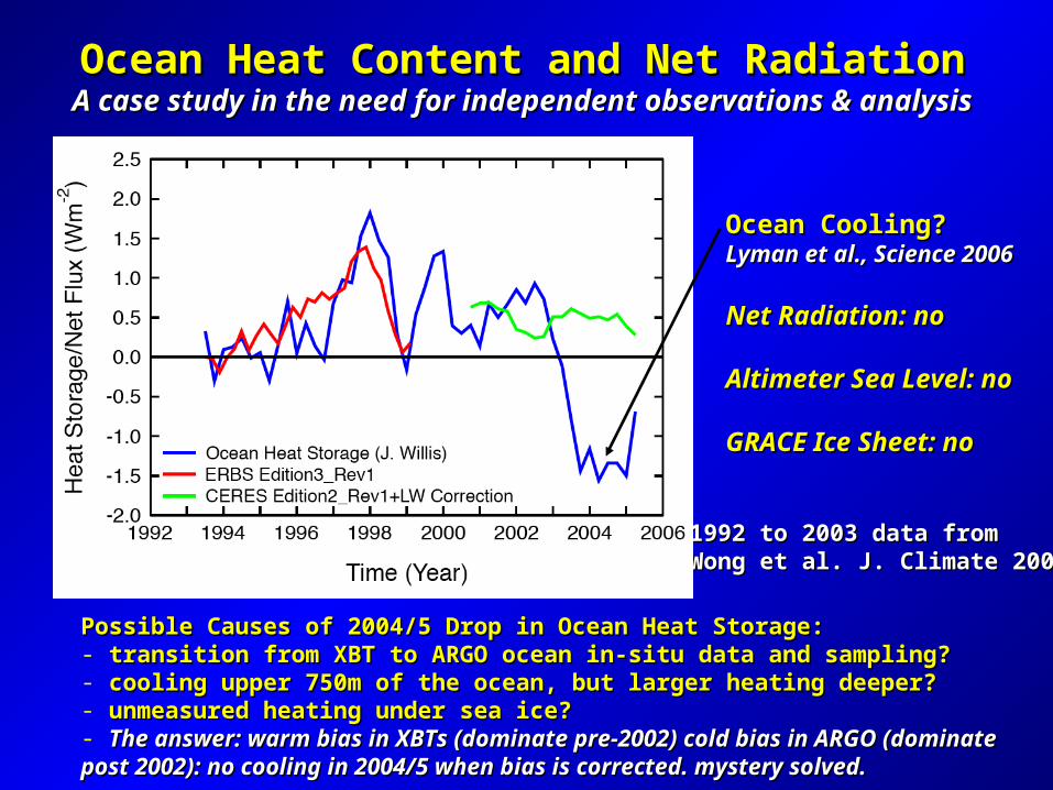
Ocean Heat Content and Net RadiationOcean Heat Content and Net RadiationA case study in the need for independent observations & analysisA case study in the need for independent observations & analysis

Possible Causes of 2004/5 Drop in Ocean Heat Storage:Possible Causes of 2004/5 Drop in Ocean Heat Storage:- transition from XBT to ARGO ocean in-situ data and sampling?transition from XBT to ARGO ocean in-situ data and sampling?- cooling upper 750m of the ocean, but larger heating deeper?cooling upper 750m of the ocean, but larger heating deeper?- unmeasured heating under sea ice?unmeasured heating under sea ice?- The answer: warm bias in XBTs (dominate pre-2002) cold bias in ARGO (dominate The answer: warm bias in XBTs (dominate pre-2002) cold bias in ARGO (dominate post 2002): no cooling in 2004/5 when bias is corrected. mystery solved.post 2002): no cooling in 2004/5 when bias is corrected. mystery solved.

Ocean Cooling?Ocean Cooling?Lyman et al., Science 2006Lyman et al., Science 2006

Net Radiation: noNet Radiation: no

Altimeter Sea Level: noAltimeter Sea Level: no

GRACE Ice Sheet: noGRACE Ice Sheet: no

1992 to 2003 data from1992 to 2003 data fromWong et al. J. Climate 2006Wong et al. J. Climate 2006

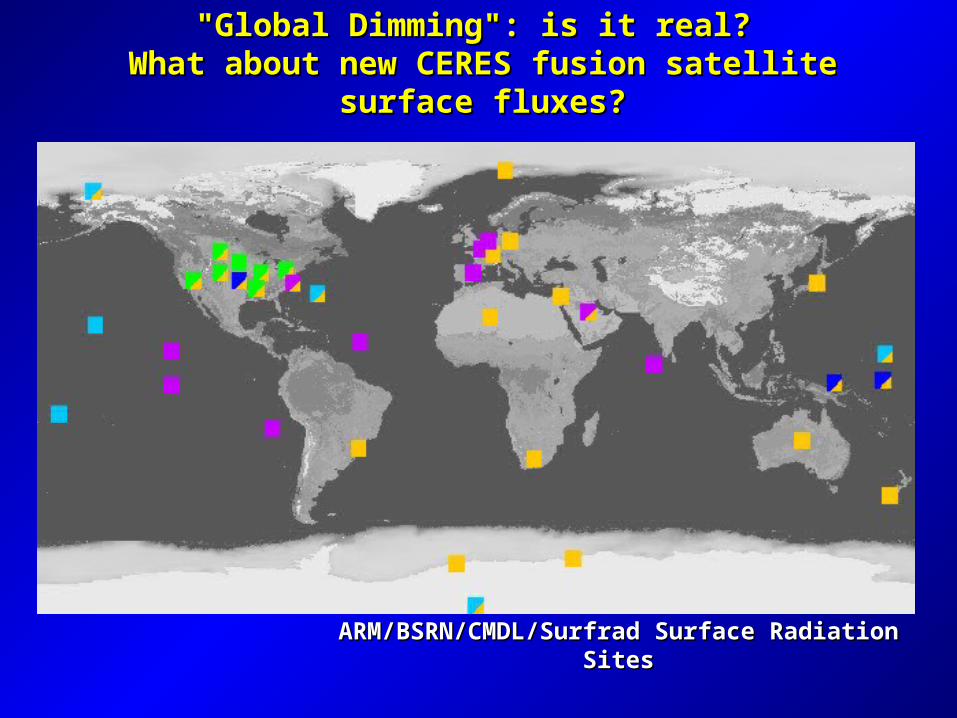
"Global Dimming": is it real? "Global Dimming": is it real? What about new CERES fusion satellite surface fluxes?What about new CERES fusion satellite surface fluxes?

ARM/BSRN/CMDL/Surfrad Surface Radiation SitesARM/BSRN/CMDL/Surfrad Surface Radiation Sites

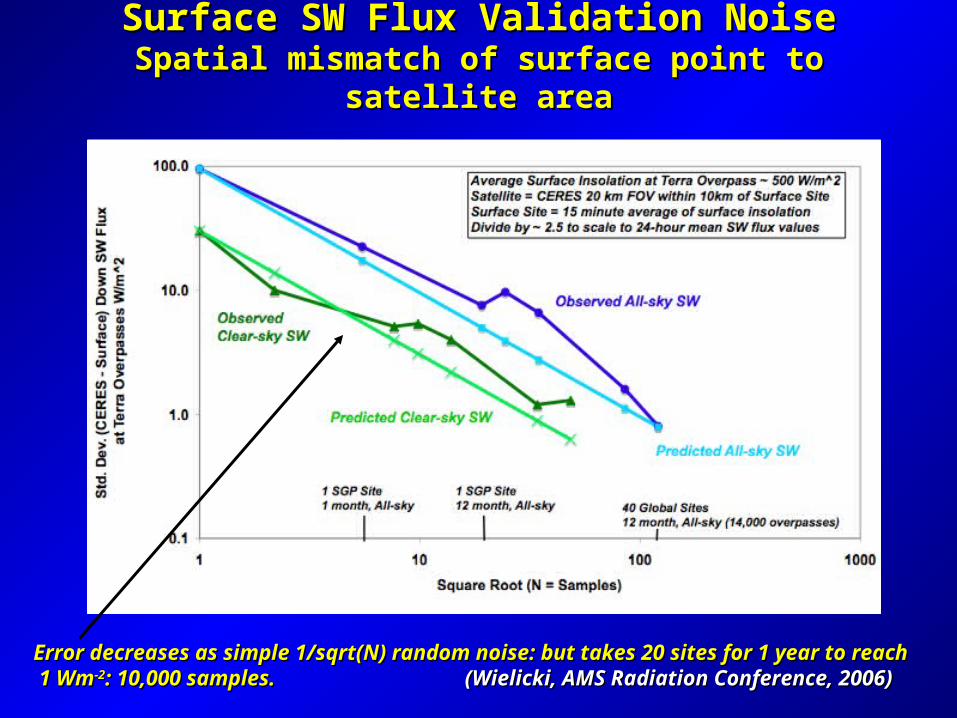
Surface SW Flux Validation NoiseSurface SW Flux Validation NoiseSpatial mismatch of surface point to satellite areaSpatial mismatch of surface point to satellite area

Error decreases as simple 1/sqrt(N) random noise: but takes 20 sites for 1 year to reachError decreases as simple 1/sqrt(N) random noise: but takes 20 sites for 1 year to reach 1 Wm 1 Wm-2-2: 10,000 samples. : 10,000 samples. (Wielicki, AMS Radiation Conference, 2006) (Wielicki, AMS Radiation Conference, 2006)

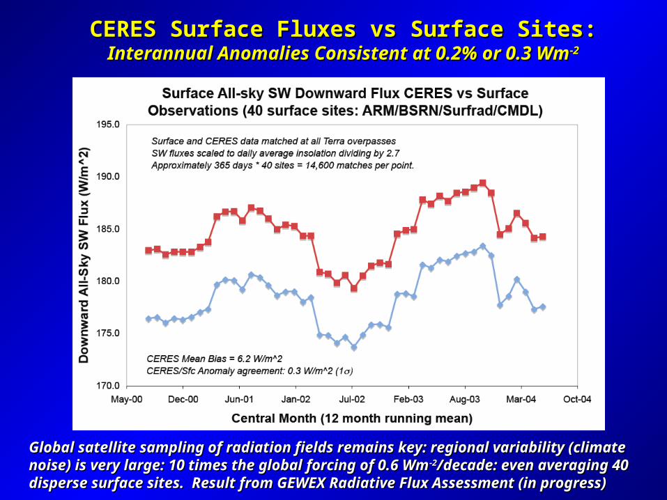
CERES Surface Fluxes vs Surface Sites:CERES Surface Fluxes vs Surface Sites:Interannual Anomalies Consistent at 0.2% or 0.3 WmInterannual Anomalies Consistent at 0.2% or 0.3 Wm-2-2

Global satellite sampling of radiation fields remains key: regional variability (climate Global satellite sampling of radiation fields remains key: regional variability (climate noise) is very large: 10 times the global forcing of 0.6 Wmnoise) is very large: 10 times the global forcing of 0.6 Wm-2-2/decade: even averaging 40 /decade: even averaging 40 disperse surface sites. Result from GEWEX Radiative Flux Assessment (in progress) disperse surface sites. Result from GEWEX Radiative Flux Assessment (in progress)

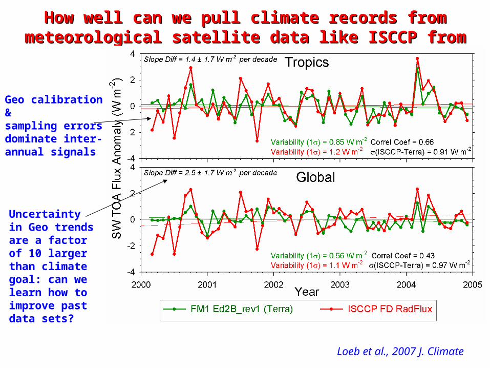
How well can we pull climate records from meteorological How well can we pull climate records from meteorological satellite data like ISCCP from geostationary?satellite data like ISCCP from geostationary?

Loeb et al., 2007 J. Climate

Geo calibration &sampling errors dominate inter-annual signals

Uncertainty in Geo trends are a factor of 10 larger than climate goal: can we learn how to improve past data sets?

Trend in All-sky Downward SW flux at the Surface (2000-2004)ISCCP vs CERES

CERES (SRBAVG_GEO) ISCCP minus CERES

- ISCCP trends show systematic regional patterns that coincide with the area of coverage by the individual GEO instruments.

- Artifacts in the GEO data are removed in CERES processing by a normalization procedure that corrects for GEO calibration, narrow-to-broadband, and radiance-to-flux coversion errors, so that fluxes from each GEO instrument are consistent with CERES.

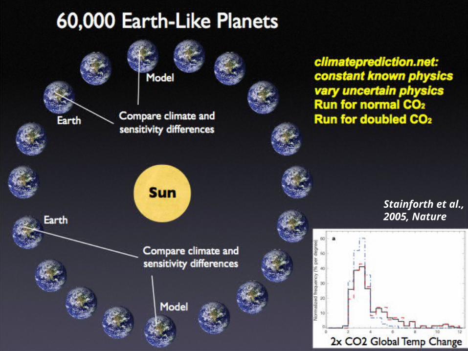
Stainforth et al.,2005, Nature

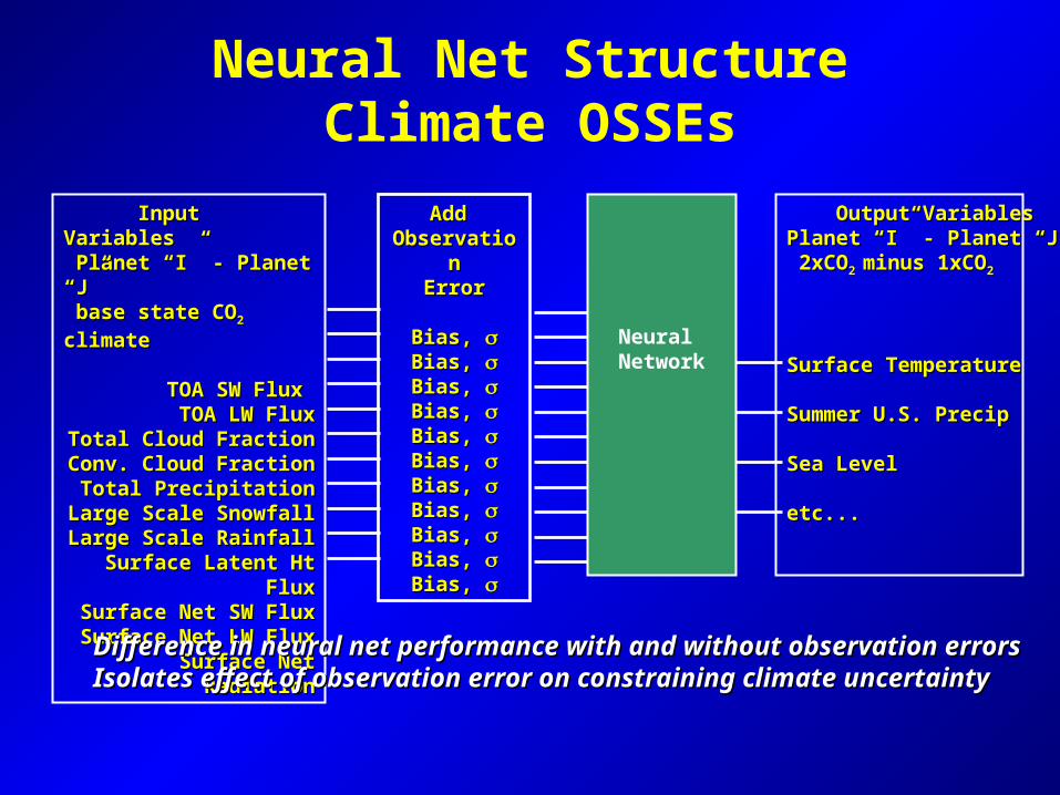
Neural Net StructureClimate OSSEs

Input VariablesInput Variables Planet “I” - Planet “J” Planet “I” - Planet “J” base state CObase state CO2 2 climateclimate

TOA SW Flux TOA SW Flux TOA LW FluxTOA LW Flux

Total Cloud FractionTotal Cloud FractionConv. Cloud FractionConv. Cloud Fraction

Total PrecipitationTotal PrecipitationLarge Scale SnowfallLarge Scale SnowfallLarge Scale RainfallLarge Scale Rainfall

Surface Latent Ht FluxSurface Latent Ht FluxSurface Net SW FluxSurface Net SW FluxSurface Net LW FluxSurface Net LW Flux

Surface Net RadiationSurface Net Radiation

Neural Network

Output VariablesOutput VariablesPlanet “I” - Planet “J”Planet “I” - Planet “J” 2xCO2xCO2 2 minus 1xCOminus 1xCO22

Surface TemperatureSurface Temperature

Summer U.S. PrecipSummer U.S. Precip

Sea LevelSea Level

etc...etc...

Add Add ObservationObservation

ErrorError

Bias, Bias, Bias, Bias, Bias, Bias, Bias, Bias, Bias, Bias, Bias, Bias, Bias, Bias, Bias, Bias, Bias, Bias, Bias, Bias, Bias, Bias,

Difference in neural net performance with and without observation errorsDifference in neural net performance with and without observation errorsIsolates effect of observation error on constraining climate uncertaintyIsolates effect of observation error on constraining climate uncertainty

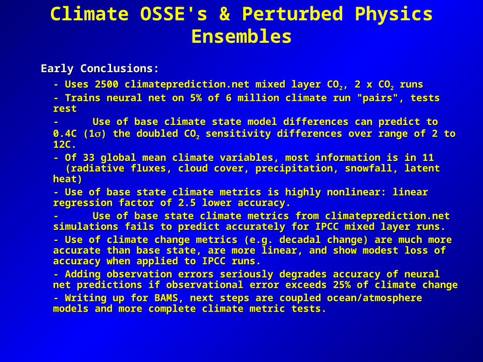
Climate OSSE's & Perturbed Physics Ensembles

Early Conclusions: Early Conclusions:

- Uses 2500 climateprediction.net mixed layer CO- Uses 2500 climateprediction.net mixed layer CO22, 2 x CO, 2 x CO22 runs runs

- Trains neural net on 5% of 6 million climate run "pairs", tests rest- Trains neural net on 5% of 6 million climate run "pairs", tests rest-- Use of base climate state model differences can predict to 0.4C Use of base climate state model differences can predict to 0.4C (1(1) the doubled CO) the doubled CO22 sensitivity differences over range of 2 to 12C. sensitivity differences over range of 2 to 12C.

- Of 33 global mean climate variables, most information is in 11- Of 33 global mean climate variables, most information is in 11 (radiative fluxes, cloud cover, precipitation, snowfall, latent heat) (radiative fluxes, cloud cover, precipitation, snowfall, latent heat)- Use of base state climate metrics is highly nonlinear: linear regression - Use of base state climate metrics is highly nonlinear: linear regression factor of 2.5 lower accuracy. factor of 2.5 lower accuracy. -- Use of base state climate metrics from climateprediction.net Use of base state climate metrics from climateprediction.net simulations fails to predict accurately for IPCC mixed layer runs.simulations fails to predict accurately for IPCC mixed layer runs.- Use of climate change metrics (e.g. decadal change) are much more - Use of climate change metrics (e.g. decadal change) are much more accurate than base state, are more linear, and show modest loss of accurate than base state, are more linear, and show modest loss of accuracy when applied to IPCC runs. accuracy when applied to IPCC runs. - Adding observation errors seriously degrades accuracy of neural net - Adding observation errors seriously degrades accuracy of neural net predictions if observational error exceeds 25% of climate changepredictions if observational error exceeds 25% of climate change- Writing up for BAMS, next steps are coupled ocean/atmosphere - Writing up for BAMS, next steps are coupled ocean/atmosphere models and more complete climate metric tests. models and more complete climate metric tests.