CLIMATE CHANGE IN THE

HEADWATERS OF THE

MEDINA RIVER

WATERSHED BAEN 673 Final Report

JASON MURRAY

Texas A&M University

Formatting:

Journal of Hydrometeorology

1

Abstract

Global climate change is a growing concern for water resources. Many water resources

are strained more and more every year due to constant increases in population. Lake Medina in

south central Texas and to the west of San Antonio is one example as it has been nearly

completely drained for municipal water supply. In this study the headwaters of the Medina River

are modeled using the Soil and Water Assessment Tool to examine the effect that climate change

will have on the river basin and ultimately to attempt to predict the future of Lake Medina. It was

shown that a climate change scenario of a 5°C temperature increase and 20% rainfall reduction

in spring and fall, a 10% reduction in summer, and a 5% reduction in fall would result in a 53%

reduction of streamflow from the observed streamflow between 1983 and 2014. Additionally a

non-climate change scenario was ran in that the climate change scenario was a 39% reduction of

streamflow.

1. Introduction

Global climate change is expected to cause alterations to the hydrology of many different

regions on different levels. There are many climate scenarios that are primarily based upon the

future greenhouse gas emissions. Some common changes are shifts in precipitation patterns,

increased average global temperatures, changes in runoff timing and magnitude, and changes to

streamflow volume (Meehl, 2007; USGCRP, 2009; Moss et al., 2010). This creates uncertainty

for water resources in regions that will be receiving decreased amounts of precipitation and even

more so if that region is also prone to drought.

Two commonly used climate scenarios are the B1 and A2 scenarios. The B1 scenario

uses ongoing globalization and predicts a future world that doesn’t have as much difference

2

between regions while the A2 scenario accounts for regional differences in socioeconomic

factors, environmental development, and other differences (Zhang et al., 2007). One common

major predicted change is the increase of average surface air temperatures (Figure 1) (USGCRP,

2009). Another major commonly predicted change is a shift in precipitation patterns where some

areas are expected to receive less precipitation while other areas are expected to receive more

precipitation (Figure 2) (USGCRP, 2009).

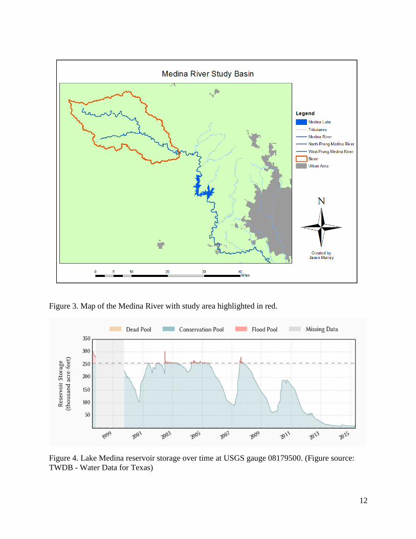
The river basin examined in this study is the Medina River, HUC 12100302, located in

south central Texas and has a total drainage area of 474 mi2. The study area is that of the

headwaters of the Medina River upstream of Lake Medina (Figure 3) that represents a 328 mi2

drainage area. The Medina River flows from the northwest of San Antonio, TX down to the west

of San Antonio then curves to the south of San Antonio where it empties into the San Antonio

River. The river is used as a water source for the San Antonio Water System (SAWS) that is

contracted for 19,974 acre-feet per year from Lake Medina (SAWS, 2012). As a result of the

current ongoing drought the water level of the reservoir has been near empty at about 3-4%

(Figure 4) because there is not adequate streamflow to fill the reservoir as well as providing the

water supply for San Antonio.

As a result of the reservoir remaining near empty for so long the tourism of the area has

decreased and is near non-existent. This has raised questions about whether the local tourism-

driven economy surrounding Lake Medina would be able to return following the drought, but

this question cannot be adequately addressed while uncertainties surrounding climate change and

how it would affect the river basin. In addition to future climate being an issue, the San Antonio

region had a population of 2,460,599 people and is projected to grow to about 4.3 million by

2060 (Vaughan et al., 2012). This creates a greater need of understanding what the future of the

3

Medina River may be so policy makers and water resources specialists have the greatest ability

to enact plans that will make the best use of the resources they have.

Using climate change scenario projections have been successfully implemented into the

Soil and Water Assessment Tool (SWAT) for the purpose of analyzing changes to streamflow

(Zhang et al., 2007; Lu et al., 2010). Zhang et al. (2007) found that within the Luohe River Basin

the analyzed climate change scenarios would not cause a dramatic change in streamflow but did

find that there would be some variability in streamflow of ±20% for most months. Lu et al.

(2010) successfully modeled the upper Mississippi River basin using SWAT and found that

monthly changes to temperature and precipitation were important, but temperature changes

dominated model outputs for future predictions. Therefore, for this study the SWAT model is

implemented in an attempt to quantify possible effects of increasing temperatures and decreased

rainfall due to climate change on the streamflow of the Medina River’s headwaters as a result of

climate change.

II. Methods

a. SWAT model

To model the Medina River headwaters this study utilized the SWAT version 2012, a

watershed-scale hydrological model, which subdivides a watershed into smaller subbasins that

represent the contributing area of a segment of stream and divides those subbasins even

hydrologic response units (HRUs) that represent a combination of land use, soil, and slope

(Arnold et al. 2012). The SWAT model delineates a watershed based upon a source digital

elevation model (DEM) raster and also uses the DEM for calculating a stream network using

flow accumulation. To compare the generated flowlines to the actual flow lines shapefiles of

4

flow lines and stream gage locations were downloaded from the USGS National Hydrography

Dataset (NHD).

b. SWAT setup and input data

The DEM raster grid was obtained from the National Elevation Dataset with a 30m

resolution. Two DEM rasters were combined using ArcMap 10.1 and the mosaic Raster tool. To

increase the speed of delineation an arbitrarily drawn mask was applied around the desired study

area. The land use data was obtained from the National Land Cover Database 2001 and soils data

was loaded from the SWAT provided ArcSWAT US STATSGO database.

The model delineated an area of the headwaters that was 328 mi2 and the outlet position

was manually chosen to be aligned with United States Geological Survey (USGS) stream gauge

08180500 Medina River at Bandera, TX. Initially the stream network was calculated with a flow

accumulation of 1000, 1500, and 2000 hectares. This flow accumulation proved to be too

minimal as the resulting stream network was overly complex and not representative of the actual

stream network and all attempts at calibration were met with failure. Following this, the stream

network was calculated with a flow accumulation area of 5000 hectares which gave more

favorable results as shown in Figure 5.

To define the HRUs the land use, soil class, and slope class percentages were all set to

10%. Slope was defined with four classes first being 0-8, second being 16-24, and fourth being

24-9999. The results of the HRU definitions are shown in Table 1 for land use, soils is reported

in Table 2, and slope classes are reported in Table 3.

Precipitation data was obtained from the National Climatic Data Center for station

GHCND:USC00415742 - Medina 1 NE, TX US. There were several periods where the station

5

had no data, so the data was filled in with -99.0 for these days. The built-in weather generator

WGEN_US_COOP_1980_2010 was used to generate all other weather data.

c. SWAT default, calibration, and validation runs

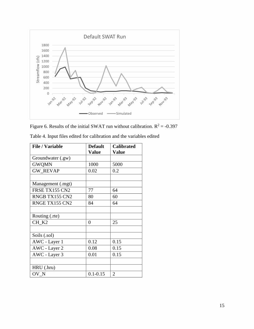
The default SWAT run was ran from 1988 to 1993 and the first 3 years were discarded

due to aquifer filling. The streamflow results of the initial SWAT run were compared to the

observed streamflow from January 1992 to December 1993 and the using Equation 1 we find the

Nash-Sutcliffe Coefficient of Suitability (R2) was -0.397 (Figure 6). An R2 of 0.5 or greater is

considered to be a suitable simulated result. Therefore, calibration was necessary to improve the

model results.

To calibrate the model the following input files were edited: groundwater (.gw), HRU

(.hru), management (.mgt), routing (.rte), and soils (.sol). The parameters that were edited in

these input files for all subbasins and their values are reported in Table 4. After calibration the

model was ran and the resulting R2 value was 0.671 (Figure 7) for validation the model was ran

from January 1, 1994 to December 31, 1999 and the resulting R2 was 0.613 (Figure 8).

d. Climate change simulation setup

To run the SWAT model for predicting future streamflow conditions of the Medina River

the decrease in precipitation was interpolated from Figure 2. This entailed a decrease of rainfall

in winter (December, January, February) of 20%, decrease in spring (March, April, May) of

20%, decrease in summer (June, July, August) of 10%, and decrease in fall (September, October,

November) of 5%. Furthermore, a temperature increase of 5°C (Mellilo et al., 2014) was

applied. These values were implemented through the subbasins (.sub) input file’s Weather

Adjustments options. In addition to running the climate change scenario, a SWAT run was

6

conducted with no changes to the parameters to simulate as if there is no climate change

occurring for the sake of comparison. The SWAT weather generator was used to generate future

weather. The simulation was ran from 2010-2050, with the first 4 years being discarded to

prevent any interference from the aquifer filling.

III. Results and Discussion

The results of the SWAT climate change run showed a decrease in average streamflow

from the measured values of 53% and a decrease of 39% from the simulated streamflow without

climate change (Figure 9). The average streamflow of the measured data was 145.4 cfs and the

climate change scenario had an average streamflow of 68.4 cfs. This shows a drastic drop in

streamflow from the past. However, it is also apparent that the output yearly average streamflow

hydrograph does not show the same high peak years that is shown in the measured past data.

This is possibly due to the SWAT weather generator not predicting the wet years that were

observed in the past. But, it could also be that those years were anomalous of a particularly wet

period in the stream basin’s history. The hydrograph for measure data before 1983 at USGS

stream gauge 08179000 (Figure 10) which is located at Pipe Creek, about 2 miles downstream of

the gage used for this study shows less high peaks and shows a higher base flow for the 1970s

and to the end of its recordings in 1982. But before the 1970s it shows long periods of low flow

and few high flow years, but none that compare to the magnitude of high flow years shown

between 1983 and 2003. The values for this time period appear to be closer resembled by the

non-drought simulated stream flows which leads one to think that the three years of very high

stream flows in 1987, 1992, and 2002 were anomalous years.

Within the future simulated stream flows it is not unreasonable to believe that Lake

Medina could begin to be filled once again due to the historical data having similar average

7

annual flows. However, with San Antonio’s projected population growth it is also plausible that

the reservoir would see more times of emptying due to the need for municipal water supply. This

would only become more realized if periods of drought are more frequent with climate change.

IV. Conclusion

Global climate change and population growth combine to create uncertainties with

respect to the planning and management of water resources. The Medina River in south central

Texas is one such location with these growing uncertainties. Lake Medina, located on the

Medina River highlights the river basin’s uncertainty as it has been near empty from 2011 to the

present because of an ongoing drought and the water supply needs of San Antonio.

Temperatures in this location are expected to rise while rainfall is expected to decrease.

In this study the SWAT model was used to simulate a future climate change scenario to observe

the effects on the headwaters of the river, upstream of Lake Medina. The simulation results

showed a large decrease of 53% in streamflow from the previous two decades which means a

great decrease in the amount of inflow to Lake Medina. Through observing historical streamflow

data and the future simulated streamflow it can be interpreted that the period of high flow years

from 1983 to 2003 were an abnormally wet period for the watershed. Additionally, the climate

change scenario streamflow was 39% less than the simulation without climate change factors.

Simulating reservoir operations would have been a worthwhile endeavor for this study,

however, the complexity and time constraints related to setting up and running reservoir

operations in SWAT created too many obstacles that could be overcome in a timely fashion. For

adequate simulation of the reservoir operations it would be required to have minimum outflow

8

data as well as future water needs projections from the reservoir. Furthermore, not having data

on the past operations of the reservoir made calibration too difficult for this study.

While the climate change scenario for this study was one of the more severe climate

change scenarios, it is still worth noting that the non-climate change scenario showed periods of

low flow that could be considered drought conditions when compared to the current drought. As

the population of San Antonio continues to grow the water resource is expected to continue to be

stressed and the recreational use of Lake Medina may sporadically return, but may also not last

long enough for the full recreational economy to return. Further studies with more detailed

climate projection data is recommended to create projections of future conditions with greater

confidence.

9

References

Arnold, J. G., Moriasi, D. N., Gassman, P. W., Abbaspour, K. C., White, M. J., Srinivasan, R., ...

& Jha, M. K. (2012). SWAT: Model use, calibration, and validation. Transactions of the

ASABE, 55(4), 1491-1508.

Lu, E., Takle, E. S., & Manoj, J. (2010). The relationships between climatic and hydrological

changes in the Upper Mississippi River Basin: A SWAT and multi-GCM study. Journal of

Hydrometeorology, 11(2), 437-451.

Meehl, G. A. (2007). Global Climate Projections in Climate Change 2007: The physical Science

Basis: contributions of Working Group I to the Fourth Assessment Report of the

Intergovernmental Panel on Climate Change.

Moss, R. H., Edmonds, J. A., Hibbard, K. A., Manning, M. R., Rose, S. K., Van Vuuren, D. P.,

... & Wilbanks, T. J. (2010). The next generation of scenarios for climate change research and

assessment. Nature, 463(7282), 747-756.

Melillo, J. M., Richmond, T. C., & Yohe, G. W. (2014). Climate change impacts in the United

States: the third national climate assessment. US Global change research program, 841.

SAWS (2012). 2012 Water Management Plan. San Antonio Water System. San Antonio, TX,

USA.

USGCRP (2009). Global Climate Change Impacts in the United States. Thomas R. Karl, Jerry

M. Melillo, and Thomas C. Peterson (eds.). United States Global Change Research Program.

Cambridge University Press, New York, NY, USA.

Vaughan, E. G., Crutcher, J. M., Labatt III, T. W., McMahan, L. H., Bradford, B. R., & Cluck,

M. (2012). Water for Texas 2012 State Water Plan Texas Water Development Board.

Zhang, X., Srinivasan, R., & Hao, E. (2007). Predicting hydrologic response to climate change in

the Luohe River basin using the SWAT model. Transactions of the ASABE, 50(3), 901-910.

10

Figures & Tables.

Figure 1. Projected change in average surface air temperature (°F) for the end of the century

(2071-2099) under climate scenarios B1 and A2 which are lower emissions and higher emissions

respectively. (Figure source: NOAA NCDC / CICS-NC; Obtained from: Mellilo et al., 2014)

11

Figure 2. Predicted changes in seasonal precipitation under climate scenario A2 which entails

higher emissions. Northern areas in blue are expected to receive increased rainfall while southern

areas in brown are expected to receive reduced rainfall. Areas overlain with diagonal lines

indicate high confidence in predictions. (Figure source: NOAA NCDC / CICS-NC; Obtained

from Melillo et al., 2014)

12

Figure 3. Map of the Medina River with study area highlighted in red.

Figure 4. Lake Medina reservoir storage over time at USGS gauge 08179500. (Figure source:

TWDB - Water Data for Texas)

13

Figure 5. Map showing the study area of the Medina River headwaters.

14

Table 1. Land Use of the study area

LANDUSE Percent of

Watershed

Area (mi2)

Water 0.18 % 0.57666

Residential-Low Density 1.99 % 6.517147

Residential-Medium Density 0.13 % 0.414221

Residential-High Density 0.02 % 0.078635

Industrial 0.01 % 0.027689

Southwestern US (arid) Range <0.01 % 0.007384

Forest-Deciduous 5.79 % 18.98216

Forest-Evergreen 44.48 % 145.9087

Forest-Mixed 0.01 % 0.049101

Range-Brush 37.33 % 122.431

Range-Grasses 9.62 % 31.56569

Hay 0.26 % 0.839517

Agricultural - Row Crops 0.15 % 0.482519

Wetlands-Forested 0.04 % 0.129583

Table 2. Soils of the study area

SOIL Percent of

Watershed

Area (mi2)

TX022 6.8 % 22.29556

TX155 72.6 % 238.1389

TX190 11.95 % 39.20256

TX527 8.65 % 28.37301

Table 3. Slope classes of the study area

SLOPE Percent of

Watershed

Area (mi2)

0-8 36.22 % 118.7939

8-16 22.88 % 75.05517

16-24 14.33 % 46.99227

24-9999 26.58 % 87.16873

15

Figure 6. Results of the initial SWAT run without calibration. R2 = -0.397

Table 4. Input files edited for calibration and the variables edited

File / Variable Default

Value

Calibrated

Value

Groundwater (.gw)

GWQMN 1000 5000

GW_REVAP 0.02 0.2

Management (.mgt)

FRSE TX155 CN2 77 64

RNGB TX155 CN2 80 60

RNGE TX155 CN2 84 64

Routing (.rte)

CH_K2 0 25

Soils (.sol)

AWC - Layer 1 0.12 0.15

AWC - Layer 2 0.08 0.15

AWC - Layer 3 0.01 0.15

HRU (.hru)

OV_N 0.1-0.15 2

0

200

400

600

800

1000

1200

1400

1600

1800

Stre

amfl

ow

(cf

s)Default SWAT Run

Observed Simulated

16

Figure 7. SWAT Calibration results. R2=0.671

Figure 8. SWAT model validation. R2=0.613

R2 = 1 − ∑ (𝑄𝑜

𝑖 − 𝑄𝑠𝑖 )

2𝑖𝑖=1

∑ (𝑄𝑜𝑖 −𝑄𝑜

)2𝑖

𝑖=1

Equation 1. Nash-Sutcliffe Coefficient of Suitability. Where Q0 is the observed streamflow, Qs is

the simulated streamflow, and 𝑄𝑜 is the average observed streamflow.

0

200

400

600

800

1000

1200

Stre

amfl

ow

(cf

s)SWAT Calibration

Observed Simulation

0

200

400

600

800

1000

1200

1400

Stre

amfl

ow

(cf

s)

Validation

Observed Simulated

17

Figure 9. Average yearly streamflow of Medina River. Past measured and future simulated

climate scenarios. Average measured streamflow is 145.4 cfs, average climate change simulated

streamflow is 68.4 cfs, and average simulated without climate change streamflow is 112.7 cfs.

Figure 10. Historical yearly average streamflows for the Medina River at Pipe Creek. USGS stream gage

08179000. Average streamflow 148.1 cfs.

0

100

200

300

400

500

600

700

800

900

19

83

19

85

19

87

19

89

19

91

19

93

19

95

19

97

19

99

20

01

20

03

20

05

20

07

20

09

20

11

20

13

20

15

20

17

20

19

20

21

20

23

20

25

20

27

20

29

20

31

20

33

20

35

20

37

20

39

20

41

20

43

20

45

20

47

20

49

Stre

amfl

ow

(cf

s)

Year

Medina River Streamflow with Climate Scenarios

Measured Climate Change No Climate Change

0

100

200

300

400

500

600

700

800

900

Stre

amfl

ow

(cf

s)

Historical Medina River Annual Average Streamflow