Climate change impacts on potential evapotranspiration, drought,

and runoff in eastern Australia

Submitted by

Lijie Shi

Thesis submitted in fulfilment of the requirements for the degree of

Doctor of Philosophy

School of Life Sciences, Faculty of Science

University of Technology Sydney

Australia

July 2021

I

Production Note:

Signature removed prior to publication.

II

Acknowledgements The journey of PhD is a truth-seeking quest in science. It is hard to believe that mine is coming to the end. I

experienced excitement, failure, self-denial, loneliness, self-affirmation, fulfillment, appreciation and so on

during the journey. There is no doubt that the journey cultivated, honed, and refined my skills of swimming

in the pool of science. However, nothing could have been achieved without the support and guidance that the

following people have offered to me. It’s such a great honor for me to express my appreciation to them.

I am so grateful to my principal supervisor, Professor Qiang Yu. A huge thanks to him. It was him who

encouraged me to purse a PhD degree abroad. It was also him who gave me a second chance after I failed in

my application the first time. Based on my academic background, he recommended me to carry out

cooperative research with Professor De Li Liu and his team at Wagga Wagga Agricultural Institute, New

South Wales Department of Primary Industries (DPI, NSW). His insights into scientific problems and

professional guidance played a significant role in sustaining my passion in science. In summary, Professor

Qiang Yu is a wonderful career model for me to follow.

The principal research scientist Dr. De Li Liu, my co-supervisor is another key mentor I appreciated very

much. He accepted me without any hesitation or doubts the very first moment I went to study at DPI, NSW.

In the past four years, I was deeply touched by Dr. De Li Liu’s authentic passion and enthusiasm in research.

The sparkle in his eyes when he talked about science was and will always be the academic tower I can look

up to. Meanwhile, I thank Dr De Li Liu for creating an inclusive, friendly, and open-minded academic

atmosphere which I could dive in. As the mentor I directly worked with, Dr De Li Liu could not do any better

and I could not thank him more. His unselfish and genuine attitude in guiding junior researcher and his never

faded enthusiasm in science are the quality I will always pursuit in my future career. I also appreciate Dr De

Li Liu’s wife, Dr Fang for so many meals she prepared during Chinese New Year or other holidays. They

were not only a feast to me but also an important emotion carrier linking with my home country, China.

I am also indebted to Dr. Bin Wang, one of my supervisors at DPI, NSW. In addition to being my supervisor,

Dr. Bin Wang is also a trustworthy brother to me. He always offered constructive suggestions to make my

research better and always encouraged me to think out of box. He is always industrious but does not push

you to be as hard working as himself. His work is always brilliant but he never judged me for not as good as

him. As a junior, Dr. Bin Wang is a dreamboat-supervisor. I deeply appreciated his insights into science and

selfless help in my study. Without his favor, nothing I have achieved today would be impossible.

III

In addition to the outstanding supervisor panels, I also appreciated my fellows from UTS, Puyu Feng, Hong

Zhang, Mingxi Zhang, Siyi Li, Dr. Jie He, Song Leng, Yuxia Liu, Dr. Rong Gan, and Dr. Qinggaozi Zhu. My

life abroad in the past four years could have been tedious and boring. However, these fellows made it colorful

and amusing. What’s more, they, especially Puyu Feng, Hong Zhang, and Mingxi Zhang also offered tons of

help in my research work. They were able to feel what I felt as the suitors of a PhD degree. Therefore, their

suggestion was very straightforward and easy to following, which were valuable to me. There is no doubt

that I will treasure the beautiful times we spend together for the rest of my life. Meanwhile, the following

visiting scholars at DPI, NSW, namely Dr. Hongtao Xing, Dr. Weiwei Xiao, and Dr. Dengpan Xiao also

enriched my life at Wagga and broaden my horizon in scientific world. I am grateful to Dr. James Cleverly

from University of Technology Sydney and Quanxiao Fang and Linchao Li from Northwest A & F University.

Their contribution to my scientific writing and data analyzing skills are tremendous.

I also appreciate staffs in UTS and DPI, NSW for their administrative assistance in many aspects, which

guaranteed an enjoyable working environment and convenient workflow. I acknowledge the financial support

I received from University of Technology Sydney and Chinese Scholarship Council, Ministry of Education,

China.

Lastly, I would love to thank my beloved family both in China and from Wagga Wagga Baptist Church. Their

unfailing love is a huge encouragement to me. My parents Benyong Shi and Hongrong Jiao, without their

support, I cannot stand the emotional struggle during the journey.

IV

Publications arising from this thesis Journal papers directly included in this thesis

1. Lijie Shi, Puyu Feng, Bin Wang, De Li Liu, James Cleverly, Quangxiao Fang, and Qiang Yu. "Projecting

potential evapotranspiration change and quantifying its uncertainty under future climate scenarios: A case

study in southeastern Australia" Journal of Hydrology, 584 (2020), DOI:

https://doi.org/10.1016/j.jhydrol.2020.124756. (Chapter 4)

2. Lijie Shi, Puyu Feng, Bin Wang, De Li Liu, and Qiang Yu. "Quantifying future drought change and associated

uncertainty in southeastern Australia with multiple potential evapotranspiration models." Journal of

Hydrology, 590 (2020), DOI: https://doi.org/10.1016/j.jhydrol.2020.125394. (Chapter 5)

Peer-reviewed international conference proceedings

1. Lijie Shi, Puyu Feng, Bin Wang, De Li Liu, Siyi Li, Qiang Yu. ‘Modelling impacts of climate change

on potential evapotranspiration in New South Wales, Australia’ The 23rd International Congress on

Modelling and Simulation (MODSIM), Canberra, Australia, 3-8 December 2019. (Extended Abstract,

Accepted).

V

Contents

Certificate of Original Authorship .................................................................................................

Acknowledgements ............................................................................................................................................................... II Publications arising from this thesis ............................................................................................................................... IV

Contents .................................................................................................................................................................................. V

List of Figures .................................................................................................................................................................... VIII

List of Tables ...................................................................................................................................................................... XIV

Abbreviations ...................................................................................................................................................................... XV

Abstract ................................................................................................................................................................................ XVI

Chapter 1. Introduction ........................................................................................................................................................ 1

1.1 Brief research background .................................................................................................................................. 1

1.1.1 Evapotranspiration response to climate change in Australia .......................................................... 1

1.1.2 Drought and aridity in Australia ............................................................................................................ 1

1.1.3 Water scarcity in Australia ...................................................................................................................... 3

1.2 Scientific problems and objectives .................................................................................................................... 3

1.3 Significance and outline of this thesis .............................................................................................................. 4

1.4 Reference ................................................................................................................................................................. 7

Chapter 2. Literature review ............................................................................................................................................... 9

2.1 Climate change....................................................................................................................................................... 9

2.1.1 Extreme climate events under a warming climate ......................................................................... 10

2.1.2 Climate change in Australia ................................................................................................................ 11

2.2 Evapotranspiration ............................................................................................................................................. 11

2.2.1 Models used in estimating evapotranspiration ................................................................................ 13

2.2.2 Response of evapotranspiration to climate change ........................................................................ 14

2.2.3 Projection of evapotranspiration under future climate scenarios................................................ 15

2.3 Drought and its response to climate change ................................................................................................. 16

2.3.1 Drought and aridity ............................................................................................................................... 16

2.3.2 Drought and aridity indices ................................................................................................................. 17

2.3.3 Impacts of climate change on drought .............................................................................................. 18

2.4 Runoff and its response to climate change ................................................................................................... 19

2.4.1 Runoff in hydrological cycle and its simulation ............................................................................. 19

2.4.2 Impacts of climate change on runoff ................................................................................................. 21

2.5 Reference .............................................................................................................................................................. 22

Chapter 3. Performance of potential evapotranspiration models across different climatic zones in New South Wales, Australia .................................................................................................................................................................. 31

3.1 Introduction.......................................................................................................................................................... 31

3.2 Study area and climate datasets....................................................................................................................... 35

3.3 Estimation of potential evapotranspiration ................................................................................................... 38

3.3.1 Penman model ........................................................................................................................................ 38

3.3.2 Temperature-based ETp models ......................................................................................................... 40

3.3.3 Radiation-based ETp models .............................................................................................................. 41

VI

3.3.4 Mass transfer-based ETp models ....................................................................................................... 42

3.4 Models’ performance in estimating ETp rates ............................................................................................. 42

3.5 Models’ ability in capturing ETp dynamics and periodic oscillations ................................................... 43

3.6 Results ................................................................................................................................................................... 45

3.6.1 Performance of models in estimating ETp rates ............................................................................. 45

3.6.2 Ability of alternative models in capturing the dynamics of ETp ................................................ 51

3.6.3 Ability of alternative models to analyze the periodicity in ETp ................................................. 54

3.7 Discussion ............................................................................................................................................................ 55

3.8 Conclusions.......................................................................................................................................................... 57

3.9 Reference .............................................................................................................................................................. 59

Chapter 4. Projecting potential evapotranspiration change and quantifying its uncertainty under future climate scenarios: A case study in southeastern Australia ....................................................................................................... 65

4.1 Introduction.......................................................................................................................................................... 66

4.2 Study area ............................................................................................................................................................. 69

4.3 Climate data and downscaling method applied ........................................................................................... 71

4.4 Empirical ETp models and random forest-based ETp models ................................................................ 74

4.5 Model evaluation ................................................................................................................................................ 77

4.6 Future ETp projection ....................................................................................................................................... 78

4.8 Results ................................................................................................................................................................... 78

4.8.1 Performance of ETp models during the historical period ............................................................ 78

4.8.2 The change of climatic factors under future climate scenarios ................................................... 80

4.8.3 ETp and its change under future climate scenarios ....................................................................... 84

4.8.4 Contribution of climatic factors to ETp change ............................................................................. 86

4.8.5 Contribution of different sources to the uncertainty of ETp projections .................................. 87

4.9 Discussion ............................................................................................................................................................ 88

4.10 Conclusions ................................................................................................................................................................ 91

4.11 Reference............................................................................................................................................................ 92

Chapter 5. Quantifying future drought change and associated uncertainty in southeastern Australia with multiple potential evapotranspiration models .............................................................................................................. 97

5.1 Introduction.......................................................................................................................................................... 98

5.2 Study sites .......................................................................................................................................................... 101

5.3 Climatic data ...................................................................................................................................................... 103

5.4 Calculation of potential evapotranspiration ............................................................................................... 105

5.5 Calculation of standardized precipitation evapotranspiration index .................................................... 106

5.6 Contribution analysis of uncertainty in future drought projection ........................................................ 108

5.7 Results ................................................................................................................................................................. 108

5.7.1 Droughts occurring in the historical period ................................................................................... 108

5.7.2 Projected changes of climatic factors under future scenarios ................................................... 110

5.7.3 Projected changes of potential evapotranspiration under future climate scenarios .............. 112

5.7.4 Projected changes in drought frequency and their relationship with climatic factors ......... 114

5.7.5 Uncertainty analysis in drought projection .................................................................................... 119

5.8 Discussion .......................................................................................................................................................... 120

5.9 Conclusions........................................................................................................................................................ 124

5.10 Reference ......................................................................................................................................................... 125

VII

Chapter 6. Subtle difference observed in runoff projection with different potential evapotranspiration inputs based on Xinanjiang model ............................................................................................................................................ 131

6.1 Introduction........................................................................................................................................................ 132

6.2 Materials and methods .................................................................................................................................... 135

6.2.1 Study area .............................................................................................................................................. 135

6.2.2 Xinanjiang (XAJ) model .................................................................................................................... 136

6.2.3 Climate data and observed runoff .................................................................................................... 138

6.2.4 The remote sensing-based evapotranspiration product and empirical ETp models ............. 139

6.2.5 Calibration and validation of XAJ model ...................................................................................... 140

6.2.6 Evaluation of model performance .................................................................................................... 140

6.2.7 Partitioning uncertainty to different sources ................................................................................. 141

6.3 Results ................................................................................................................................................................. 141

6.3.1 ETp calculated with empirical models PML_V2 ......................................................................... 141

6.3.2 XAJ model calibration and cross-model validation ..................................................................... 142

6.3.3 Changes in rainfall and evapotranspiration under future climate scenarios ........................... 146

6.3.4 Changes in soil moisture under future climate scenarios ........................................................... 148

6.3.5 Changes in runoff under future climate scenarios at different time scales ............................. 149

6.3.6 Uncertainty in runoff projection ....................................................................................................... 151

6.4 Discussion .......................................................................................................................................................... 152

6.5 Conclusion ......................................................................................................................................................... 154

6.6 Reference ............................................................................................................................................................ 155

Chapter 7. Summary and future research .................................................................................................................... 160

7.1 Summary ............................................................................................................................................................ 160

7.2 Limitations and future research ..................................................................................................................... 162

7.3 Reference ............................................................................................................................................................ 163

VIII

List of Figures Figure 1-1. Examples of damage caused by major drought happened in Australia. The figure is extracted

from Mpelasoka et al. (2008) ........................................................................................................................... 2

Figure 1-2. Flow chart of this project ...................................................................................................................... 6

Figure 3-1 The distribution of 2120 stations and the division of climate zones in NSW based on the aridity index (rainfall/potential evapotranspiration). ............................................................................... 36

Figure 3-2 Scatter plot with daily ETp from 1970 to 2014 at eight stations belonging to arid (Tibooburra & Wilcannia), semi-arid (Cobar & Gunnedah), sub-humid (Murrurundi & Paterson), and humid (Coffs Harbour & Sydney) zones. ETp_observed (mm day-1) represents daily ETp estimated with Penman, WMO, Mahringer (Mah), and Trabert (Tra) based on observed wind speed whereas ETp_2m/s (mm day-1) represents daily ETp estimated with the corresponding models (Penman2, WMO2, Mah2, and Tra2) based on the recommended wind speed, 2 m s-1. The red line is the 1:1 line. ...................................................................................................................................................................... 38

Figure 3-3 Scatter plot between annual ETp estimated by Penman model (ET-Penman, mm year-1) and ET0 estimate by Penman-FAO56 (ET-FAO56, mm year-1) at four climate zones from 1970 to 2014. .............................................................................................................................................................................. 39

Figure 3-4 Models’ ability in estimating daily ETp, shown by Taylor diagram. Taylor diagram displayed the performance of 12 ETp models in terms of amplitude of their variations (the radial distance from the origin the points was proportional to the pattern standard deviations) and their correlation coefficients (given by the azimuthal position of the test field) against Penman-calculated ETp. The dark red lines represented the skill scores. The data used to plot the Taylor diagrams was the averaged daily ETp for each climate zone from 1970 to 2014. The X-axis and Y-axis both represented standard deviations (SDs) of ETp. The column of S in this figure was daily Taylor skill score for each model. ...................................................................................................................................... 46

Figure 3-5 The distribution of nRMSE (%) between daily ETp estimated by simplified ETp models and ETp estimated by Penman model from 1970 to 2014. Data used for each climate zone is the daily nRMSE of stations locating in this zone, that is, 201 stations for arid zone, 980 stations for semi-arid zone, 536 stations for sub-humid zone, and 403 stations for humid zone. The upper and lower box boundaries indicate the 75th and 25th percentiles; the black line and the black dot within the box represents the median and mean value, respectively; the upper and lower whiskers are the 10th and 90th percentiles. The hollow boxes represented for the radiation-based models. The red boxes were for temperature-based models and the purple boxes represented for the mass transfer-based models................................................................................................................................................................. 47

Figure 3-6 Distribution of rMBE (%) between daily ETp estimated by simplified ETp models and ETp estimated by Penman model from 1970 to 2014. Data used for each climate zone is the daily rMBE (%) of stations locating in this zone, that is, 201 stations for arid zone, 980 stations for semi-arid zone, 536 stations for sub-humid zone, and 403 stations for humid zone. The upper and lower box boundaries indicate the 75th and 25th percentiles; the black line and the black dot within the box represents the median and mean value, respectively; the upper and lower whiskers are the 10th and 90th percentiles. The hollow boxes represented for the radiation-based models. The red boxes were for temperature-based models and the purple boxes represented for the mass transfer-based models. .............................................................................................................................................................................. 48

Figure 3-7 Models’ ability in estimating seasonal ETp, shown by Taylor diagram. The data used to plot

IX

the Taylor diagrams was the averaged seasonal ETp for each climate zone from 1970 to 2014. The column of S in this figure was seasonal Taylor skill scores for each model. Other explanations of Taylor diagram were the same with Figure 3-4. ....................................................................................... 49

Figure 3-8 The distribution of nRMSE (%) between seasonal ETp estimated by simplified ETp models and ETp estimated by Penman model from 1970 to 2014. Data used for each climate zone is the seasonal nRMSE of stations locating in this zone, that is, 201 stations for arid zone, 980 stations for semi-arid zone, 536 stations for sub-humid zone, and 403 stations for humid zone. The explanation of boxes was the same with that in Figure 3-5. .................................................................. 50

Figure 3-9 Distribution of rMBE (%) between seasonal ETp estimated by simplified ETp models and ETp estimated by Penman model from 1970 to 2014. Data used for each climate zone is the seasonal rMBE (%) of stations locating in this zone, that is, 201 stations for arid zone, 980 stations for semi-arid zone, 536 stations for sub-humid zone, and 403 stations for humid zone. The explanation of boxes was the same with that in Figure 3-5. .................................................................. 51

Figure 3-10 Temporal evolution of ETp estimated by 13 models from 1970 to 2014 for each climate zone. .................................................................................................................................................................... 52

Figure 3-11 The temporal trends of precipitation both for seasonal and annual scales at four climate zones in the research period from 1970 to 2014. ...................................................................................... 53

Figure 3-12 The temporal trends of annual ETp (mm year-1) estimated by 13 models at four climate zones in the research period from 1970 to 2014. The asterisk symbol (*) showed the significant level. *: significant at 95% confidence level; **: significant at 99% confidence level. ................. 53

Figure 3-13 The temporal trends of seasonal ETp (mm year-1) estimated by 13 models at four climate zones in the research period from 1970 to 2014. The asterisk symbol (*) had the same meaning with that in Figure 3-12. ................................................................................................................................. 54

Figure 3-14 The wavelet-spectra and variances of annual ETp estimated by 13 models at four climate zones. The thin solid lines denote the cones of influence, and the thick solid lines show the 95% confidence levels. The colour bar means the vibration intensity of the periods at different timescales. .............................................................................................................................................................................. 55

Figure 4-1 The location of eight stations in four different climate zones across New South Wales, Australia, and their elevations (m) determined by digital elevation model (DEM). The climate dividing lines have the same meaning with that in Figure 3-1 and is developed based on the widely used aridity index (rainfall/ETp) (UNESCO, 1979) ................................................................................ 70

Figure 4-2 Flow diagram of the random forest model. ..................................................................................... 76

Figure 4-3 The average annual ETp (mm year-1) calculated by eight ETp models for each station during the model testing period (2001 - 2014). The dashed lines and red bars indicate the average annual ETp calculated by the Penman-Monteith model. ..................................................................................... 79

Figure 4-4. Scatter plots of the Penman-calculated daily ETp (mm day-1) vs ETp calculated by RF-based and empirical ETp models during the model testing stage (2001 - 2014) for each of eight stations in New South Wales, Australia. The units for RMSE and rMBE are mm day-1 and %, respectively. Blue lines are linear regression lines and red lines are 1:1 lines. .......................................................... 80

Figure 4-5. Projected changes in Tmax (℃), Tmin (℃), and Tmax-Tmin (℃) in the near future (2026 – 2050, 2040s), the medium future (2051 – 2075, 2065s), and the far future (2076 – 2100, 2090s) at eight stations in New South Wales, Australia, under RCP4.5 and RCP8.5 scenarios based on 34 GCMs compared with baseline values (1990 - 2014). Lower and upper box boundaries indicate the 25th and 75th percentiles, respectively. The black lines and dots inside the box mark the median

X

and mean, respectively. The lower and upper whiskers indicate the 10th and 90th percentiles, respectively. ....................................................................................................................................................... 82

Figure 4-6. Projected changes in Rs (MJ m-2 day-1), and rainfall (mm year-1) in the near future (2026 – 2050, 2040s), the medium future (2051 – 2075, 2065s), and the far future (2076 – 2100, 2090s) at eight stations in New South Wales, Australia, under RCP4.5 and RCP8.5 scenarios based on 34 GCMs compared with baseline values (1990 - 2014). Lower and upper box boundaries indicate the 25th and 75th percentiles, respectively. The black lines and dots inside the box mark the median and mean, respectively. The lower and upper whiskers indicate the 10th and 90th percentiles, respectively ........................................................................................................................................................ 83

Figure 4-7. Projected ETp changes for eight stations in New South Wales, Australia in the near future (2026 - 2050, 2040s), the medium future (2051 - 2075, 2065s), and the far future (2076 - 2100, 2090s) under RCP4.5 and RCP8.5 scenarios based on 34 GCMs compared with baseline ETp (1990 - 2014). Lower and upper box boundaries indicate the 25th and 75th percentiles, respectively. The black lines and dots inside the box mark the median and mean, respectively. The lower and upper whiskers indicate the 10th and 90th percentiles, respectively. .............................................................. 85

Figure 4-8 25-year averaged annual ETp (mm year-1) at eight stations for the near future (2026 – 2050, 2040s), the medium future (2051 – 2075, 2065s), and the far future (2076 – 2100, 2090s) under RCP4.5 and RCP8.5. Box boundaries indicate the 25th and 75th percentiles; the black lines and dots inside the box mark the median and mean, respectively; the lower and upper whiskers indicate the 10th and 90th percentiles, respectively. ............................................................................................... 85

Figure 4-9 Regression coefficients for changes in ETp (ΔETp, mm year-1) with changes in maximum temperature (ΔTmax, ℃), minimum temperature (ΔTmin, ℃), solar radiation (ΔRs, MJ m-2 day-

1), and rainfall (ΔP, mm year-1) in a multiple liner regression model (ΔETp = a ΔTmax+b ΔTmin+c ΔRs+d ΔP); units for a and b are mm year-1 oC-1; units for c are mm year-1 (MJ m-2 d-1)-1; units for d are mm year-1 mm-1. ***:p < 0.001, **:p < 0.01; *:p < 0.05 ............................................................. 87

Figure 4-10. The contribution of uncertainty sources to the change of ETp. .............................................. 88

Figure 5-1 Location of the two study sites in the wheat belt of New South Wales (NSW), Australia.102

Figure 5-2 The qq-plots between simulated SPEI driven by downscaled climatic data from 34 GCMs and observed SPEI driven by observed climatic data from SILO at Gunnedah (the upper panels, a) and Wagga Wagga (the bottom panels, b) under RCP4.5 (left panels) and RCP8.5 (right panels) scenarios. RF1, RF2, and RF3 (random forest models 1, 2, and 3, respectively); JH (Jensen-Haise); Mak (Makkink); HS (Hargreaves); Ab (Abtew). Abbreviations above the individual panels refer to specific GCMs. ............................................................................................................................................... 104

Figure 5-3 Frequency of seasonal droughts occurring in the period from 1971 to 2010 at Gunnedah and Wagga Wagga, Australia, using eight potential evapotranspiration models. RF1, RF2, and RF3 (random forest models 1, 2, and 3, respectively); JH (Jensen-Haise); Mak (Makkink); HS (Hargreaves); Ab (Abtew). Mild, moderate, and severe drought classifications are based on Standardized Precipitation Evapotranspiration Index values as described in section 5.5. Drought refers to the total of all drought classifications. ...................................................................................... 109

Figure 5-4 Mean seasonal potential evapotranspiration (ETp, mm year-1) from 1971 to 2010 at Gunnedah and Wagga Wagga, Australia calculated by eight ETp models. RF1, RF2, and RF3 (random forest models 1, 2, and 3, respectively); JH (Jensen-Haise); Mak (Makkink); HS (Hargreaves); Ab (Abtew). ........................................................................................................................... 110

Figure 5-5 Projected changes in maximum (Tmax, °C, a1, a2) and minimum (Tmin, °C, b1, b2) air

XI

temperature, solar radiation (Rs, MJ m-2 day-1, c1, c2), and precipitation (P, %, d1, d2) in the 2040s and 2080s at Gunnedah (a1, b1, c1, d1) and Wagga Wagga (a2, b2, c2, d2), Australia, under RCP4.5 and RCP8.5 scenarios. Lower and upper box boundaries indicate the 25th and 75th percentiles, respectively. The black line and dot inside each box indicate the median and mean, respectively. The lower and upper whiskers indicate the 10th and 90th percentiles, respectively. ..................... 111

Figure 5-6 Projected changes in potential evapotranspiration (ETp, %) in the near future (2021-2060, 2040s) and further future (2061-2100, 2080s) at Gunnedah and Wagga Wagga, Australia, under RCP4.5 and RCP8.5 scenarios based on 34 GCMs compared with baseline values (1971-2010). Lower and upper box boundaries indicate the 25th and 75th percentiles, respectively. The black line and dot inside each box mark the median and mean, respectively. The lower and upper whiskers indicate the 10th and 90th percentiles, respectively. .............................................................................. 113

Figure 5-7 Regression coefficients for changes in ETp (ΔETp, %) at Gunnedah and Wagga Wagga, southeast Australia, with changes in Tmax (ΔTmax, °C), Tmin (ΔTmin, °C), and Rs (ΔRs, MJ m-2 day-1) in a multiple liner regression model (ΔETp (%) = a0*ΔTmax (°C) + b0*ΔTmin (°C)+ c0*ΔRs (MJ m-2 day-1)) for seven ETp models; ***:p < 0.001, **:p < 0.01; *:p < 0.05. RF1, RF2, and RF3 (random forest models 1, 2, and 3, respectively); JH (Jensen-Haise); Mak (Makkink); HS (Hargreaves); Ab (Abtew). Units for a0 and b0 are % °C-1; units for c0 are % (MJ m-2 day-1)-1. The color legend represents the values of a0, b0, and c0. ............................................................................. 114

Figure 5-8 Changes in the frequency of seasonal mild drought (upper left panels, -1 < SPEI <= -0.5), moderate drought (upper right panels, -1.5 < SPEI <= -1), severe drought (lower left panels, SPEI <= -1.5), and the total drought (SPEI <= -0.5) in the near (2021 – 2060, 2040s) and further (2061 – 2100, 2080s) future periods compared with the baseline period (1971 - 2010) at Gunnedah and Wagga Wagga, Australia. The calculation of SPEI was based on seven ETp models driven by downscaled climatic data from 34 GCMs under RCP4.5 and RCP8.5 scenarios. Data presented are changed mean frequency in the 40-year values for the 34 GCMs compared with that of the baseline period. RF1, RF2, and RF3 (random forest models 1, 2, and 3, respectively); JH (Jensen-Haise); Mak (Makkink); HS (Hargreaves); Ab (Abtew). .................................................................................... 116

Figure 5-9 Changes in the frequency of seasonal mild drought (upper left panels, -1 < SPEI <= -0.5), moderate drought (upper right panels, -1.5 < SPEI <= -1), severe drought (lower left panels, SPEI <= -1.5), and the total drought (lower right panels, SPEI <= -0.5) in the near (2021-2060, 2040s) and further (2061 – 2100, 2080s) future periods compared with the baseline period (1971 - 2100) at Gunnedah and Wagga, Australia. The calculation of SPEI was based on seven ETp models driven by downscaled climatic data from 34 GCMs under RCP4.5 and RCP8.5 scenarios. Data presented are changed frequency in the 40-year values for each of the 34 GCMs compared with that of the baseline period. Lower and upper box boundaries indicate the 25th and 75th percentiles, respectively. The black line and dot inside each box mark the median and mean, respectively. The lower and upper whiskers indicate the 10th and 90th percentiles, respectively. RF1, RF2, and RF3 (random forest models 1, 2, and 3, respectively); JH (Jensen-Haise); Mak (Makkink); HS (Hargreaves); Ab (Abtew). RF1, RF2, and RF3 (random forest models 1, 2, and 3, respectively); JH (Jensen-Haise); Mak (Makkink); HS (Hargreaves); Ab (Abtew). ................................................ 117

Figure 5-10 Regression coefficients for changes in frequency of seasonal droughts (ΔF, %) at Gunnedah and Wagga Wagga, Australia with changes in precipitation (ΔP, %) and potential evapotranspiration (ΔETp, %) in a multiple liner regression model (ΔF (%) = a*ΔP (%) + b*ΔETp (%)) for seven ETp models; ***:p < 0.001, **:p < 0.01; *:p < 0.05. RF1, RF2, and RF3 (random forest models 1, 2,

XII

and 3, respectively); JH (Jensen-Haise); Mak (Makkink); HS (Hargreaves); Ab (Abtew). Coefficients a and b are dimensionless. The color legend represents the values of a and b. ........ 118

Figure 5-11 Contribution (%) of GCMs, RCPs, and ETp models to the uncertainty in drought frequency projection at Gunnedah and Wagga Wagga, Australia for each season. Results for mild, moderate, and severe drought are shown from inward to outward circles, respectively. Contributions larger than 15% are shown by numbers in the figure. ....................................................................................... 120

Figure 6-1 Location of the North Johnstone River catchment, Queesland, Australia and the distribution of 10 weather stations and the location of Tung Oil gauge (a hydrologic gauge station). ............ 135

Figure 6-2 The flow chart for the XAJ model. ................................................................................................. 137

Figure 6-3 Scatter plots of the daily ETa (mm day-1) estimated by PML_V2 vs ETp estimated by empirical ETp models from 2000 to 2017 for each of ten stations in North Johnstone river catchment, Queensland, Australia. The units for RMSE is mm day-1. The red and the blue lines represent the 1:1 lines and the linear regression lines, respectively. .................................................. 142

Figure 6-4 The observed daily runoff and the simulated daily runoff by XAJ model with calibrated parameters of Ab model (as in Table 6-1) during calibration (2000-2010) and validation (2011-2017) periods in the North Johnstone catchment. .................................................................................. 145

Figure 6-5 The annual historical observed and simulated runoffs with calibrated parameters shown in Table 1 in the North Johnstone river basin. The bar plot (second-y-axis) showed the bias error (simulated runoff-observed runoff)/observed runoff*100) between simulated runoff and observed runoff. ............................................................................................................................................................... 146

Figure 6-6 Projected seasonal changes in rainfall (%) in the near future (2021-2040, 2030s), middle future (2041-2060, 2050s), far future (2061-2080, 2070s), and further future (2081-2100, 2090s) under RCP4.5 and RCP8.5 scenarios based on 34 GCMs compared with the baseline period (2001-2020). The upper and lower box boundaries indicate the 75th and 25th percentiles; the black line and the black dot within the box represents the median and mean value, respectively; the upper and lower whiskers are the 10th and 90th percentiles. .................................................................................. 147

Figure 6-7 Projected seasonal changes in ETp (%) and ETa (%) for different ETp models in the near future (2021-2040, 2030s), middle future (2041-2060, 2050s), far future (2061-2080, 2070s), and further future (2081-2100, 2090s) under RCP4.5 and RCP8.5 scenarios based on 34 GCMs compared with the baseline period (2001-2020). The upper and lower box boundaries indicate the 75th and 25th percentiles; the black line and the black dot within the box represents the median and mean value, respectively; the upper and lower whiskers are the 10th and 90th percentiles. 148

Figure 6-8 Projected seasonal changes in soil moisture for different layers, namely the upper soil layer (0 - 20 cm), the lower soil layer (20 – 50 cm), and the deepest soil layer (> 50 cm) in the near future (2021-2040, 2030s), middle future (2041-2060, 2050s), far future (2061-2080, 2070s), and further future (2081-2100, 2090s) under RCP4.5 and RCP8.5 scenarios based on 34 GCMs compared with the baseline period (2001-2020). The upper and lower box boundaries indicate the 75th and 25th percentiles; the black line and the black dot within the box represents the median and mean value, respectively; the upper and lower whiskers are the 10th and 90th percentiles ................................ 149

Figure 6-9 Projected seasonal changes in runoff (%) for different ETp models in the near future (2021-2040, 2030s), middle future (2041-2060, 2050s), far future (2061-2080, 2070s), and further future (2081-2100, 2090s) under RCP4.5 and RCP8.5 scenarios based on 34 GCMs compared with the baseline period (2001-2020). The upper and lower box boundaries indicate the 75th and 25th percentiles; the black line and the black dot within the box represents the median and mean value,

XIII

respectively; the upper and lower whiskers are the 10th and 90th percentiles ................................ 150

Figure 6-10 Pearson correlation coefficients for the relation between runoff and its related factors. The purple color showed negative correlation while the red color showed the positive correlation. . 151

Figure 6-11 The relative contribution of GCMs, RCPs, ETp models and their interactions to the uncertainty caused in runoff projection for each season. ...................................................................... 152

XIV

List of Tables Table 3-1. The mean minimum (Tmin) and maximum (Tmax) air temperature, solar radiation (Rs),

relative humidity (RH), rainfall (P), potential evapotranspiration (ETp), and aridity index (AI) in the study period from 1970 to 2014. ............................................................................................................ 36

Table 4-1 Geographical and long-term average meteorological information for eight stations locating in for different climate zones across New South Wales, Australia. The values in parentheses are the standard deviations for each variable .......................................................................................................... 71

Table 4-2 Identifying information for 34 global climate models (GCMs). GCMs were used for statistically downscaling outputs for eight stations across New South Wales, Australia, under the RCP4.5 and RCP8.5 scenarios. ..................................................................................................................... 73

Table 4-3. The input requirements of seven ETp models used in this study. .............................................. 77

Table 5-1 Geographical and long-term averaged meteorological information for Gunnedah and Wagga Wagga, Australia. The geographical information includes longitude (Lon), latitude (Lat), and elevation (DEM). The meteorological information includes air temperature (T), solar radiation (Rs), relative humidity (RH), wind speed (Wind), precipitation (P), and potential evapotranspiration (ETp). ................................................................................................................................................................ 103

Table 5-2 Potential evapotranspiration (ETp) models used in this study. The Penman model was used as the benchmark to develop and train the RF-based models and to assess the performance of the RF-based and the empirical ETp models. ETp estimated by the four empirical ETp models was compared with ETp estimated by the RF-based models which required the same inputs. Specifically, JH and Mak were compared with RF1; HS was compared with RF2; and Ab was compared with RF3. ................................................................................................................................................................... 105

Table 5-3 Variance inflation factors (VIF) to choose independent factors for multiple linear regression. ............................................................................................................................................................................ 118

Table 6-1 Geographical and the multi-year (2001-2017) mean meteorological information in the research period for ten stations in North Johnstone catchment. .......................................................... 136

Table 6-2 The 16 calibrated parameters and their value that were good for all ETp models to produce the best runoff simulation in the North Johnstone river catchment. The values of parameters were the results of cross-model validation. ........................................................................................................ 138

Table 6-3 Group of parameters calibrated with ETp estimated by different models to drive XAJ model. ............................................................................................................................................................................ 143

Table 6-4 The R2, NSE, and RMSE between observed runoff and simulated runoff with the six groups of parameters shown in Table 6-3. The ETp model that was used to calibrated XAJ model was marked as red during cross-model validation. The unit for RMSE is mm day-1. .......................... 144

XV

Abbreviations BoM Bureau of Meteorology

CR Capillary rise

DP Deep percolation

ET Evapotranspiration

ETa Actual evapotranspiration

ETp Potential evapotranspiration

ET0 Reference evapotranspiration

H Sensible heat of water

I Irrigation water

G Soil heat flux

GCMs Global Climate Models

P Precipitation

XAJ Xinanjiang model

RCPs Representative Concentration Pathways

Rn Net radiation

RO Runoff

R Surface runoff

SILO Science

SPEI Standardized precipitation evapotranspiration index

λ Latent heat of vaporization

△SF Horizontal surface flow

△SW Change in soil moisture

XVI

Abstract As one of the most arid continents, Australia is exposed to drought and water scarcity. The changing

climate is likely to intrigue more drought occurrence and make water scarcity more severe. In this context, it

is important to investigate the influence of climate change on drought and water availability in Australia.

This study aimed to investigate the possible change of potential evapotranspiration (ETp), drought

occurrence, and runoff under future climate scenarios, thus providing useful information to mitigate the

adverse impacts of climate change on crop production and water resource management. In specific, four

inter-related studies were carried out based on widely used empirical ETp models, random forest method,

statistical indices, standardized precipitation evapotranspiration index (SPEI), Xinanjiang model, and a three-

way analysis of variance. Findings from these studies suggested that: (1) radiation based models including

Jensen-Haise, Abtew, modified Makkink, and Turc and temperature-based model Hargreaves were able to

reasonably estimate ETp rates, capture its temporal evolution, and periodically oscillation; (2) random forest-

based ETp models generally outperformed empirical ETp models which required the same climatic inputs;

(2) ETp was likely to increase in the future and the increase could be mostly explained by the increase in

temperature and solar radiation; (3) Droughts, especially for moderate and severe droughts were also likely

to increase and the increases in spring and winter were larger than that in summer and autumn. The increase

in ETp explained more of the change in drought than the decrease in rainfall did; (4) There were obvious

decreases in spring and winter runoff whereas the mean changes in summer and autumn runoff were subtle.

The changes in runoff were consistent with the pattern of changes in rainfall and the difference in ETp inputs

barely influenced runoff projection; (5) GCMs, RCPs, or their interaction generally were the dominant factors

resulting in uncertainty in the projections of ETp, drought, and runoff in future climate scenarios.

This study confirmed the increase in air evaporative demand, drought occurrence, and water scarcity in

eastern Australia and highlighted the necessary to for farmers and policy makers take measures to adapt to

the changing climate. The possible measures include cultivating drought-resistant varieties, adjusting the

planting structure, improving the capability of drought forecast, and changing the seeding windows

accordingly.

Keywords：climate change; potential evapotranspiration; random forest, drought; runoff; uncertainty;

eastern Australia

1

Chapter 1. Introduction

1.1 Brief research background

1.1.1 Evapotranspiration response to climate change in Australia

Climate change has been verified in the last century in Australia and it is going to continue in the

following decades (CSIRO and BOM, 2015). In specific, temperature has increased by 0.9°C in Australia in

the past hundred years (CSIRO and BOM, 2015); wind speed has decreased over 90% of Australia (McVicar

et al., 2008) while rainfall did not show uniform trend across Australia.

Companied with climate change, evapotranspiration (ET) inevitably showed temporal evolution. As an

illustration, Kirono et al. (2009) analyzed the temporal evolution of Pan-evaporation and point potential

evaporation in Australia from 1970 to 2004, claiming that both pan evaporation and point potential

evaporation showed general increasing trend. Similarly, CSIRO and BOM (2015) also demonstrated that

Morton point potential evaporations has increased in the last hundred years and will keep increasing in the

future based on the output from global climate models (GCMs). Another example is that Kirono and Kent

(2011) reported that most regions in Australia are going to experience increasing evapotranspiration.

Consequently, the areas influenced by drought is going to increase by 1.4% to 16.8% to 2070 over the Eastern

NSW region. In addition to increasing trend in evaporation, negative trend has also been found across

Australia since 1970 (Jovanovic et al., 2008; Kirono and Jones, 2007; McVicar et al., 2008; Roderick and

Farquhar, 2004; Roderick et al., 2007).

The obvious discrepancy will have impact on the confidence in model projections. Meanwhile, in spite

of the fact that evapotranspiration could be estimated based on pan evaporation, evapotranspiration by which

90% of rainfall returns back to atmosphere in Australia (Rayner, 2007) is different with pan evaporation to

some extent (Johnson and Sharma, 2010). However, research directly focusing on evapotranspiration

response to climate change in Australia is still scare. Thus, both the discrepancy and the gap highlight the

importance to do further research on evapotranspiration impact of climate change to reconcile the differences

between estimation from models or instrumental records.

1.1.2 Drought and aridity in Australia

Drought is a recurring climate event in Australia (Bond et al., 2008). For instance, the most recent one,

2

known as “millennium” drought has lasted more than ten years from 1996 to 2010 (Steffen, 2015). Similar

to other natural disaster, drought has remarkably influence on ecosystem, agricultural production, economic

and social activities and so on (Mishra and Singh, 2010). As reported, drought happened in Australia resulted

in a 36% reduction in winter cereal crop, thus leaving many framers in financial crisis in 2006 (Wong et al.,

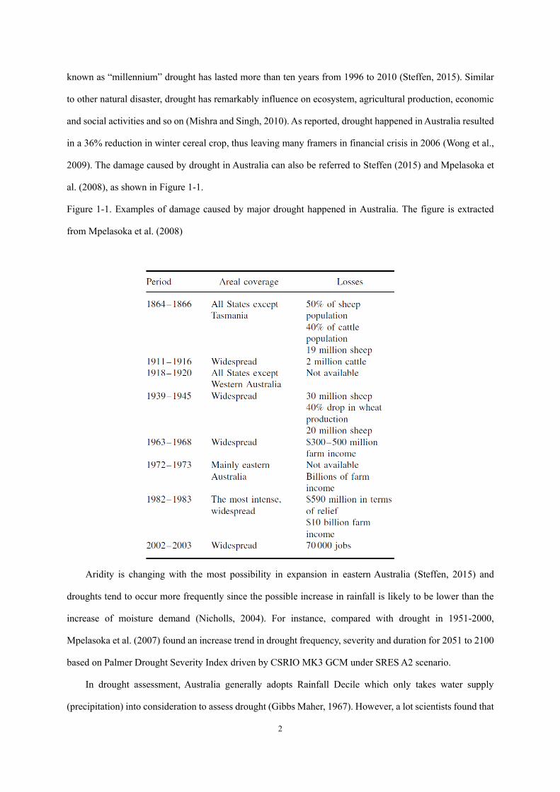
2009). The damage caused by drought in Australia can also be referred to Steffen (2015) and Mpelasoka et

al. (2008), as shown in Figure 1-1.

Figure 1-1. Examples of damage caused by major drought happened in Australia. The figure is extracted

from Mpelasoka et al. (2008)

Aridity is changing with the most possibility in expansion in eastern Australia (Steffen, 2015) and

droughts tend to occur more frequently since the possible increase in rainfall is likely to be lower than the

increase of moisture demand (Nicholls, 2004). For instance, compared with drought in 1951-2000,

Mpelasoka et al. (2007) found an increase trend in drought frequency, severity and duration for 2051 to 2100

based on Palmer Drought Severity Index driven by CSRIO MK3 GCM under SRES A2 scenario.

In drought assessment, Australia generally adopts Rainfall Decile which only takes water supply

(precipitation) into consideration to assess drought (Gibbs Maher, 1967). However, a lot scientists found that

3

the increasing frequency of drought occurrence is due to the increase in evapotranspiration instead of the

decrease in precipitation. In this case, the index only involving precipitation in assessing drought might lead

to misunderstanding on the cause of drought and may underestimate the possible increase of draught

frequency. For example, Mpelasoka et al. (2008) compared Rainfall Deciles and Soil Moisture Deciles

(considering both precipitation and evapotranspiration) in assessing drought in Australia and claimed that

thought both drought indexes draw consistent conclusion on a general increase in drought frequency over

Australia, the increases detected by Soil Moisture Deciles are larger than that detected by Rainfall Deciles.

More than that, they argued that the Soil Moisture Deciles is more relevant to resource management and

evapotranspiration is more important in determining the severity of droughts in a warming world (Mpelasoka

et al., 2008). Therefore, it sounds reasonable to adopt a relative comprehensive drought index to project

drought events under future climate scenarios (Asadi Zarch et al., 2015) so that results from researches with

various drought indexes could be compared and improve the reliability in adaption to potential drought events.

1.1.3 Water scarcity in Australia

Shortage in rainfall and the uneven distribution between water resource and population makes water

scarcity be a serious problem to agricultural production in Australia (Mpelasoka et al., 2007). For instance,

Murray-Darling Basin which is the center both to major urban area and agricultural production receives

around 6% of total rainfall run off in Australia (Chartres and Williams, 2006; Ejaz Qureshi et al., 2013). On

the contrary, the tropical north which is characterized with low population densities has relative abundance

of available water (Ejaz Qureshi et al., 2013). What’s more, under the ongoing climate change, rainfall has

showed declined trend (CSIRO, 2008) and most GCMs’ projections support a continuing decrease in annual

rainfall but increase in evapotranspiration in Australia (Chiew et al., 2009). Thus, the rain-fed agricultural

production system which consumes around 70% of total water consumption may be challenged by more

serious water stress in future (Adamson et al., 2009; Pigram, 2007; Wittwer and Griffith, 2011). For instance,

Ejaz Qureshi et al. (2013) reported that compared with the expected rice production in Murray-Darling Basin,

it was reduced by 70%, 20% and 10% in dry, medium and wet climate scenarios. In this circumstance, it is

important to project the potential influence of climate change on water scarcity and offer feasible measures

to offset the detriment.

1.2 Scientific problems and objectives

Around 80% of Australia continent is characterized with arid or semi-arid climate where annual rainfall

4

is less than 600mm, which makes Australia very vulnerable to climate change. Nowadays, there is a

possibility in increasing trend in water scarcity and extreme events like drought under the changing climate

(CSIRO and BOM, 2015). Thus, drought policy and water management might need to be adjusted

accordingly (Kirono and Kent, 2011).

Evapotranspiration (ET) is a key parameter in drought assessment, hydrological cycle, and water

management. As reported, the increasing evapotranspiration, which is mainly caused by global warming will

worsen the dry conditions in arid regions (Goyal, 2004; Tabari et al., 2011). Given the ongoing climate change,

it is necessary to figure out how evapotranspiration has changed in the past, its current behavior and what is

going to happen in the future climate scenarios (Kirono et al., 2009). Thorough understanding on

evapotranspiration is a prerequisite to project drought and water resource management under future climate

scenarios.

In this context, this project aims at offering a comprehensive analysis on climate change impacts on

evapotranspiration, drought and water availability in Australia from the recent past to the future (2100), thus

reveal the temporal evolution of evapotranspiration, drought, and runoff. This project is going to offer

answers to the following questions:

(1) Are the simplified empirical ETp models reliable in estimating ETp rates, detecting its temporal

trends and analyzing its interannual oscillation?

(2) What is the influence of different ETp models on drought and runoff projection and their response

to future climate change?

(3) How do factors like GCMs, RCPs, and ETp models contribute to the uncertainty in their projection?

The specific goals of this research are to:

(1) Reveal the factors driving the temporal evolution of evapotranspiration, drought, and runoff

regimes;

(2) Quantify the evapotranspiration, drought, and runoff regimes under future climate scenarios with

chosen evapotranspiration models, drought indexes, and hydrological model driven by multi-model ensemble

method.

1.3 Significance and outline of this thesis

Evapotranspiration, drought, and runoff are three inter-connected parameters, which are all deeply

influenced by climate change. Meanwhile, they can directly or indirectly exert influence on agricultural

5

production and human society especially to a water-limited country like Australia. Therefore, with climate

change going on, a thorough understanding on their temporal evolution in the past and projecting their

potential change under future climate scenarios are prerequisites to investigate the response of water

availability in the future. This PhD project which combines the concern of “Living in a changing climate”

and concern of “water availability” driven by the state-of-the-art multi-model ensemble method will provide

such insight. Results of this project are helpful to foresee potential water-stress in eastern Australia thus

formulating reasonable adaptation measures to make sure the sustainable development both in water resource

and agricultural production under a changing climate.

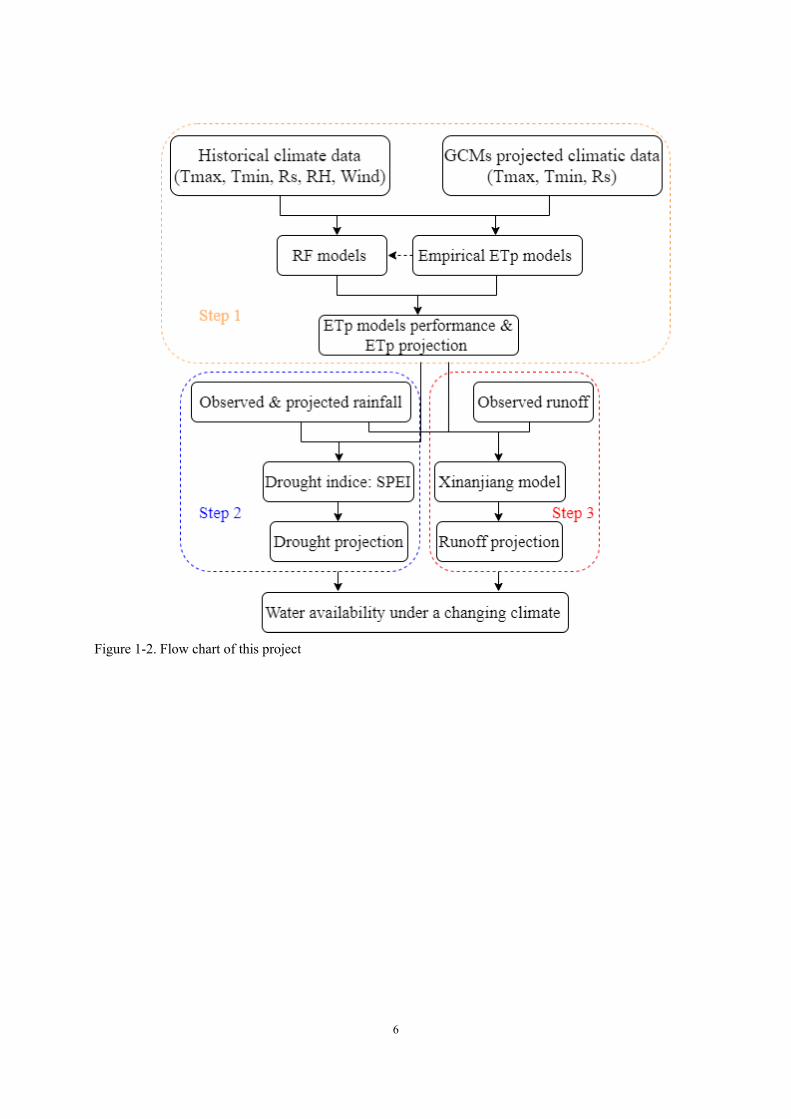
The thesis is structured as the following. First, a general introduction (Chapter 1) followed by literature

review (Chapter 2) was given to clarify the study background and its significance. Then the four mainstay

chapters aim to answer the subsequent questions: The performance of empirical ETp models across different

climatic zones (Chapter 3); The response of ETp to climate change and the uncertainty in ETp projection

(Chapter 4); The response of drought to climate change and the uncertainty in its projection based on multiple

ETp models and ensemble GCMs (Chapter 5); The response of runoff to climate change and the influence of

different ETp inputs on runoff projection (Chapter 6); Chapter 7 summarized the general conclusions,

limitations, and future research directions. Figure 1-2 showed the flow chart of the thesis.

6

Figure 1-2. Flow chart of this project

7

1.4 Reference Adamson, D., Mallawaarachchi, T., Quiggin, J., 2009. Declining inflows and more frequent droughts in the

Murray–Darling Basin: climate change, impacts and adaptation*. Australian Journal of Agricultural

and Resource Economics, 53(3): 345-366. DOI:doi:10.1111/j.1467-8489.2009.00451.x

Asadi Zarch, M.A., Sivakumar, B., Sharma, A., 2015. Droughts in a warming climate: A global assessment of

Standardized precipitation index (SPI) and Reconnaissance drought index (RDI). Journal of

Hydrology, 526: 183-195. DOI:https://doi.org/10.1016/j.jhydrol.2014.09.071

Bond, N.R., Lake, P.S., Arthington, A.H., 2008. The impacts of drought on freshwater ecosystems: an

Australian perspective. Hydrobiologia, 600(1): 3-16. DOI:10.1007/s10750-008-9326-z

Chartres, C., Williams, J., 2006. Can Australia Overcome its Water Scarcity Problems? Journal of

Developments in Sustainable Agriculture, 1(1): 17-24. DOI:10.11178/jdsa.1.17

Chiew, F.H.S. et al., 2009. Estimating climate change impact on runoff across southeast Australia: Method,

results, and implications of the modeling method. Water Resources Research, 45(10).

DOI:doi:10.1029/2008WR007338

CSIRO, 2008. Water availability in the Murray–Darling Basin. CSIRO Canberra.

CSIRO, BOM, 2015. Climate change in Australia information for Australia's natural resource management

regions: technical report, CSIRO and Bureaur of Meteorology, Australia.

Ejaz Qureshi, M., Hanjra, M.A., Ward, J., 2013. Impact of water scarcity in Australia on global food security

in an era of climate change. Food Policy, 38: 136-145.

DOI:https://doi.org/10.1016/j.foodpol.2012.11.003

Gibbs Maher, W., 1967. Rainfall deciles as drought indicators/by WJ Gibbs and JV Maher. Melbourne:

Bureau of Meteorology.

Goyal, R.K., 2004. Sensitivity of evapotranspiration to global warming: a case study of arid zone of Rajasthan

(India). Agricultural Water Management, 69(1): 1-11. DOI:10.1016/j.agwat.2004.03.014

Johnson, F., Sharma, A., 2010. A Comparison of Australian Open Water Body Evaporation Trends for Current

and Future Climates Estimated from Class A Evaporation Pans and General Circulation Models.

Journal of Hydrometeorology, 11(1): 105-121. DOI:10.1175/2009jhm1158.1

Jovanovic, B., Jones, D.A., Collins, D., 2008. A high-quality monthly pan evaporation dataset for Australia.

Climatic Change, 87(3-4): 517-535. DOI:10.1007/s10584-007-9324-6

Kirono, D., Jones, R.N., 2007. A Bivariate test for detecting inhomogeneities in pan evaporation series.

Australian Meteorological Magazine, 56(2): 93-103.

Kirono, D.G.C., Jones, R.N., Cleugh, H.A., 2009. Pan‐evaporation measurements and Morton‐point potential

evaporation estimates in Australia: are their trends the same? International Journal of Climatology,

29(5): 711-718. DOI:doi:10.1002/joc.1731

Kirono, D.G.C., Kent, D.M., 2011. Assessment of rainfall and potential evaporation from global climate

models and its implications for Australian regional drought projection. International Journal of

Climatology, 31(9): 1295-1308. DOI:doi:10.1002/joc.2165

McVicar, T.R. et al., 2008. Wind speed climatology and trends for Australia, 1975–2006: Capturing the stilling

phenomenon and comparison with near‐surface reanalysis output. Geophysical Research Letters,

35(20). DOI:doi:10.1029/2008GL035627

Mishra, A.K., Singh, V.P., 2010. A review of drought concepts. Journal of Hydrology, 391(1-2): 202-216.

DOI:10.1016/j.jhydrol.2010.07.012

Mpelasoka, F., Hennessy, K., Jones, R., Bates, B., 2008. Comparison of suitable drought indices for climate

8

change impacts assessment over Australia towards resource management. International Journal of

Climatology, 28(10): 1283-1292. DOI:doi:10.1002/joc.1649

Mpelasoka, F.S., Collier, M.A., Suppiah, R., Arancibia, J.P., 2007. Application of Palmer drought severity index

to observed and enhanced greenhouse conditions using CSIRO Mk3 GCM simulations. NSW,

410047(29.1): 5.7.

Nicholls, N., 2004. The Changing Nature of Australian Droughts. Climatic Change, 63(3): 323-336.

DOI:10.1023/B:CLIM.0000018515.46344.6d

Pigram, J., 2007. Australia's water resources: from use to management. CSIRO publishing.

Rayner, D.P., 2007. Wind Run Changes: The Dominant Factor Affecting Pan Evaporation Trends in Australia.

Journal of Climate, 20(14): 3379-3394. DOI:10.1175/jcli4181.1

Roderick, M.L., Farquhar, G.D., 2004. Changes in Australian pan evaporation from 1970 to 2002.

International Journal of Climatology, 24(9): 1077-1090. DOI:10.1002/joc.1061

Roderick, M.L., Rotstayn, L.D., Farquhar, G.D., Hobbins, M.T., 2007. On the attribution of changing pan

evaporation. Geophysical Research Letters, 34(17). DOI:doi:10.1029/2007GL031166

Steffen, W., 2015. Thirsty country: climate change and drought in Australia. Sydney, Australia: Climate

Change Council of Australia Ltd.

Tabari, H., Marofi, S., Aeini, A., Talaee, P.H., Mohammadi, K., 2011. Trend analysis of reference

evapotranspiration in the western half of Iran. Agricultural and Forest Meteorology, 151(2): 128-

136. DOI:10.1016/j.agrformet.2010.09.009

Wittwer, G., Griffith, M., 2011. Modelling drought and recovery in the southern Murray‐Darling basin*.

Australian Journal of Agricultural and Resource Economics, 55(3): 342-359.

DOI:doi:10.1111/j.1467-8489.2011.00541.x

Wong, G., Lambert, M.F., Leonard, M., Metcalfe, A.V., 2009. Drought Analysis Using Trivariate Copulas

Conditional on Climatic States. Journal of Hydrologic Engineering, 15(2): 129-141.

DOI:doi:10.1061/(ASCE)HE.1943-5584.0000169

9

Chapter 2. Literature review

2.1 Climate change

Global climate change has been demonstrated in many aspects including risen temperature, changing

precipitation patterns, more extreme climate events, warming ocean, shrinking ice sheets and so on (IPCC,

2014). In specific, temperature has increased by 0.85°C while precipitation increased in tropical areas and

decrease in the rest of the world (IPCC, 2014; Wasko et al., 2021). Globally, Kharin et al. (2013) claimed

that per degree increase in global mean temperature is likely to induce in 1.5%-2.5% increase in global mean

precipitation. In addition, both changes in temperature and precipitation are generally results of extreme

temperature events or extreme precipitation events. For instance, Westra et al. (2013) reported that the median

intensity of annual maximum daily precipitation would increase by 5.9%-7.7% per K degree increase in mean

temperature. Herold et al. (2018) projected that some regions in Australia would experience an increase up

to 3.5°C in maximum day time temperatures and all capital cities in Australia are likely to witness a triple

increases of heatwave days per year by the far future (2060-2079).

Global climate models (GCMs), which was firstly proposed by Phillips (1956) and regional climate

models (RCMs) have been widely used in climate change study and projection (Chen et al., 2012; Ekström

et al., 2007; Frei et al., 2006). Given the raw spatial resolution of data extracted from GCMs, both dynamical

and statistical downscaling method are used to bridge the gap (Hay and Clark, 2003; Wilby et al., 2000). Both

the downscaling process and structure of GCMs will produce uncertainty. In other words, uncertainty is an

inevitable problem in climate change projection. The main sources of uncertainty include the following

aspects. Firstly, the definition of the greenhouse gas emissions scenarios which is used to drive the GCMs

might vary (Wilby and Harris, 2006). Secondly, the GCMs that are developed with different model structures

may produce various climate projections even under the same emission scenario (Taylor et al., 2012). Thirdly,

the downscale methods used to downscale climatic data from GCMs to finer temporal and spatial scales to

force the evapotranspiration models is another source of uncertainty (Maraun et al., 2010; Wilby et al., 2000).

Lastly, the diverse evapotranspiration models are also an importance source of uncertainty in drought and

runoff projection (Thompson et al., 2013; Wang et al., 2015). The research of uncertainty related to

hydrological projection, climatic factors projection (such as rainfall), and extreme climate events projection

like drought have been globally reported (Brunner et al., 2021; Kauffeldt et al., 2016). For instance, Arnell

(2011) analyzed the uncertainty in projecting runoff response to climate change in UK catchments with the

10

use of data from 21 GCMs driving a hydrological model. He claimed that the change of runoff ranged from

-40% to +20% with an increase of 2◦C in mean temperature, showing great uncertainty. Similarly, Barria et

al. (2015) projected that runoff in southwestern Australian would experience a reduction ranging from 10%

to 80% as a combined result of 0% - 40% reduction in precipitation and 0.5◦C – 3◦C increase in temperature.

They claimed that the range of uncertainty in runoff projection was even larger than earlier studies (Barria et

al., 2015). However, these studies mostly focused on analyzing the widespread range of the projected items

but were weak in analyzing the contribution of different sources to the uncertainty.

2.1.1 Extreme climate events under a warming climate One of the main results caused by climate change is the increases in the occurrence and even the

concurrent of extreme climate events, such as drought, heatwaves, cold waves, frost, and flood (Hao et al.,

2013; Hao et al., 2018). These extreme climate events can have severe influence on agricultural production,

water and food security, economic, and many other aspects of human-being life and ecosystem. Take the

study of Chen et al. (2020) as an explanation, they projected the extreme climate events in the Yangtze River

Basin, China with the use of 12 extreme climate indices and analyzed their effect on maize and rice. Results

from their study showed that maize yield in this region was likely to decrease by 5.36% under RCP4.5 and

6.04 under RCP8.5. The corresponding reduction in rice yield was 2.55% and 2.48%. At global scale, Hao et

al. (2018) reported that western US, northern South America, western Europe, Africa, western Asia,

southeastern Asia, southern India, northeastern China and eastern Australia are likely to experience

significant increase in the severity of dry and hot extremes. Herold et al. (2018) demonstrated that drought

and the number of days above 30°C is expected to increase across the major wheat-belt in Australia.

Meanwhile, the increases are mainly expected in spring when wheat is most vulnerable to heat stress. All

these studies highlighted the inevitable increases of extreme climate events and the necessity of carrying out

research about them to mitigate the potential dire effects.

Drought is a natural hazard influenced by rainfall and air temperature. The occurrence of drought can

have great negative influence on many aspects of human-being life (Hao and Singh, 2015; van Kempen et

al., 2021). In the future, drought risk and severity may increase due to the warming climate (Cook et al.,

2014). As Cook et al. (2020) reported in their latest research that regions including western North America,

Central America, Europe and the Mediterranean, the Amazon, Southern Africa, China, Southeast Asia , and

Australia are going to experience strong drying. Meanwhile, the extreme drought events could increase by

11

200-300% in some regions. With more regions exposing to drought, the aridity areas are also going to shift.

In summary, there are two dominant viewpoints in aridity shift. One is the phenomenon of ‘rich-get-richer’,

that is, humid regions will be more humid while arid regions will dry out further with global warming (Chen

et al., 2017; Chou et al., 2009; Durack et al., 2012); another one supports that arid regions are becoming

slightly more humid while humid zones are most likely to become a little bit drier (Asadi Zarch et al., 2017).

In this context, the projection of drought in an arid continent is necessary for offering alarm warning and

taking early action to mitigate the potential dire effects.

2.1.2 Climate change in Australia Australia is the second most arid continent on earth and the variety of its climates makes it more

vulnerable to climate change. Climate in Australia has been warming and the warming trend will continue in

the 21th century. Accompanying with increasing of greenhouse gases emission, average near-surface air

temperature in Australia has witnessed a 0.9°C increase since 1910 (CSIRO and BOM, 2015). Meanwhile,

extreme weather events happened more frequently. Particularly, extreme heat events obviously outnumbered

extreme cool events. Since 1950, heatwaves happening in Australia were companied with the characteristic

of longer duration, higher frequency and stronger intensity. Change of rainfall in Australia showed spatial

and seasonal variation. In general, the tropical north of Australia has experienced increase in rainfall whereas

it decreased in the south of Australia since 1950 (Dey et al., 2019). Correspondingly, changes in streamflow

also showed similar spatial variation, that is, south of Australia experienced decrease in streamflow while

increasing trends were found in north of Australia (Zhang et al., 2016b). Seasonal changes in precipitation

presented as decreasing in autumn and winter rainfall while increasing in spring and summer rainfall. It is

projected that future climate in Austria will continue to experience increasing temperature with more

extremely hot days but fewer extremely cool days (Alexander and Arblaster, 2017); increasing extreme

rainfall across most of Australia but southern continental Australia may see decline of winter and spring

precipitation (CSIRO and BOM, 2015).

2.2 Evapotranspiration Evapotranspiration is the sum of evaporation, which is a process that liquid water is lost from soil surface

to water vapor in the air and transpiration which describes vaporization of water from vegetation (Allen et

al., 1998; Kool et al., 2014). The energy driven evapotranspiration, to a large degree, comes from solar

radiation, then secondly comes from air temperature (Jensen and Allen, 2015). In addition to the driving

12

energy, the gradient of water vapor pressure between the surface of evapotranspiration and the ambient

environment offers force to remove the water vapor from the evapotranspiration surface. Meanwhile, wind

helps to blow the humid air away and bring drier air, otherwise the evapotranspiration will slow down when

the surrounding air becomes more and more humid. In summary it is solar radiation, relative humidity, air

temperature and wind speed that affect the process of evapotranspiration from the perspective of meteorology

(Eslamian et al., 2011; Zhang et al., 2016a). Apart from meteorological factors, evapotranspiration is also

influenced by water availability in the soil, crop characteristics, environment and management practice

(Cammalleri et al., 2010; Rana and Katerji, 2000).

As we mentioned above, evapotranspiration is not only influenced by meteorological factors but also

crop characteristics, environment, and management. Thus, scientists defined reference evapotranspiration

(ET0), potential evapotranspiration (ETp), and actual evapotranspiration (ETa) to describe evapotranspiration

under different conditions from the perspective of parameters included. The detail definitions on ET0, ETp,

and ETa are in the following paragraph:

The ET0 is only meteorological parameters-related, representing the atmospheric power of evaporation.

It is defined as evapotranspiration rate from a reference vegetation surface which is covered with an actively

growing grass shading the ground totally, with the uniform height of 0.12m, a fixed surface resistance of 70

s m-1 and an albedo of 0.23 under no water limited condition (Allen et al., 1998). Potential evapotranspiration

is the maximum evapotranspiration rate from crop which grows in a large field under ideal environmental

and management conditions, bearing zero water stress under a given climate (Li et al., 2016). Actual

evapotranspiration is the evapotranspiration rate from crop in reality condition where water scarcity, water

logging or unideal might happen thus reducing the evapotranspiration rate (Cammalleri et al., 2010; Farg et

al., 2012).

The relationship of ET0, ETp and ETa can be described via the following equations:

0

0

(2-1)(2-2)

p c

a s p s c

ET K ETET K ET K K ET

=

= =

where Kc and Ks are crop coefficient and the adjust coefficient standing for the stress from water and

environment.

Evapotranspiration is one of the most basic and important components to hydrological, meteorological,

agricultural, and ecological communities (Gharbia et al., 2018; Jensen and Allen, 2015). In summary, the

importance of evapotranspiration mainly displays in the following aspects: (1) it is an important joint of water

13

cycle and energy balance. In specific, evapotranspiration accounts for around 67% of precipitation and

evapotranspiration is also the media through which radiation onto the earth’s surface returns back to the

atmosphere as latent and sensible heat (Fisher et al., 2017; Oki and Kanae, 2006); (2) evapotranspiration is

an important parameter in hydrological, environmental, and agricultural models; For instance, irrigation

water requirement is the difference between effective precipitation and crop water requirement which equals

to crop evapotranspiration in value. In hydrological field, evapotranspiration is involved in most hydrological

models like SWAT model.

The methods used in measuring evapotranspiration are mainly based on the theory of energy balance,

as shown in equation (2-3), and water balance, as shown in equation (2-4) and (2-5) at field or regional scale,

or mass transfer method (Jensen and Allen, 2015). Though measurement is the most direct and accurate

method in quantifying evapotranspiration, there are obvious disadvantages for this method. Generally

speaking, measuring evapotranspiration requires specific devices including lysimeters, tanks, eddy

covariance flux tower, or evaporation pan. Normally, these equipments are expensive to installation, labor

and time-consuming in management and maintenance, and needs well-trained professional personnel to cope

with. Thus, measuring evapotranspiration directly is mainly employed by research purpose (Allen et al.,

1998).

Energy balance equation:

0 (2-3)nR G ET H− − − =

where Rn (MJ m-2 day-1) represents net radiation; H (MJ m-2 day-1) represents the sensible heat; G (MJ m-2

day-1) represents the soil heat flux; Λet (MJ m-2 day-1) represents the latent heat flux, via which express the

evapotranspiration rate. is the latent heat of vaporization, equaling to 2.45 MJ kg-1 at 20 °C.

Water balance equations at field scale (2-4) and regional scale (2-5):

(2-4)(2-5)

ET I P RO DP CR SF SWET P RO

= + − − + + +

= −

where I (mm) is irrigation water, P (mm) is precipitation, RO is surface runoff (mm), DP is deep percolation

(mm), CR (mm) is capillary rise, △SF (mm) is the horizontal surface flow, △SW (mm) is the change in

soil content.

2.2.1 Models used in estimating evapotranspiration

Given the difficulty in measuring evapotranspiration directly, many models have been developed since

14

1950s to estimate it with meteorological data (Allen et al., 1998). In literature, around 50 different methods

have been reported in estimating evapotranspiration (Lu et al., 2005). In general, these models could be

classified into two types – fully physical based model and empirical/semi-empirical model. In specific,

empirical model are classified into temperature-based model (Hargreaves and Allen, 2003), radiation-based

model (Priestley and Taylor, 1972), mass transfer-based model (Mahringer, 1970) according to the climatic

factors incorporated in the model. Among all methods, Penman (Penman, 1948) and Penman-Monteith

FAO56 (PM) model are fully physiological based and takes all the related meteorological factors into

consideration. The advantage of these two models are that they are able to offer reasonable accuracy result

against measured ET independent on climate conditions, thus they can be used to any climate circumstance

without calibration (Li et al., 2016). However, meteorological factors required by them may not always be

available especially in developing countries (Tabari et al., 2013) and in future climate scenarios (Wang et al.,

2015).

As to the empirical or semi-empirical models, they are normally developed based on specific climate

conditions, thus they are normally suited to certain climates and should be tested or recalibrated when used

under a different climate (Donohue et al., 2010). As a matter of fact, cross comparison of models has been

carried out in various regions including European (Alexandris et al., 2008; Bormann, 2010), South America

(de la Casa and Ovando, 2016), Iran (Tabari, 2009; Tabari et al., 2013; Valipour et al., 2017), China (Li et al.,

2016; Li et al., 2015; Peng et al., 2017), American (Douglas et al., 2009; Lu et al., 2005), Canada (Aladenola

and Madramootoo, 2013; Sentelhas et al., 2010). Remarkable difference of model performance exists in these

studies. For instance, Valipour et al. (2017) assessed the performance of 15 ET models against PM across

various climates in Iran. They found that model Abtew (Ab) has a better performance than other ET modes

in semiarid climate; While, Hargreaves performs best in very humid regions and the Mediterranean. Still in

different climates of Iran, Tabari (2010) investigated the performance of four ET models (Turc, Makkink, PT

and Hargreaves) which are all included in research of Valipour et al. (2017). But he claimed that Hargreaves

model outperforms other models under semi-arid and warm humid climate. Thus, it is still a necessary to do

location-specific research to choose a best performed simplified ET model at a certain region.

2.2.2 Response of evapotranspiration to climate change

Both positive and negative trends have been noticed in evapotranspiration due to climate change

(Dinpashoh et al., 2011; Gao et al., 2017b). The unexpected decreasing evapotranspiration with increasing

15

temperature has been famous known as “evaporation paradox” (Brutsaert and Parlange, 1998; Roderick and

Farquhar, 2002). Air temperature is not the only one factors influencing evapotranspiration, thus the positive

effect caused by increasing temperature could be masked by the negative influence of other climatic factors.

For instance, Donohue et al. (2010) demonstrated that the contribution of temperature, wind speed, solar

radiation and vapor pressure to evapotranspiration change magnitude were 1.5 mm year-1, -1.3 mm year-1, -

0.6 mm year-1, and -0.4 mm year-1, respectively. Obviously, the reduced rates caused by wind speed, solar

radiation and vapor pressure pronounced more than air temperature did, resulting in a general downward

trend in evapotranspiration. In summary, the possible reasons caused decrease in evapotranspiration include

(1) the shrunk difference range of diurnal temperature (Roderick and Farquhar, 2002); (2) the global dimming

due to increase in aerosol and cloudiness (Fan et al., 2016; Huo et al., 2013; Roderick and Farquhar, 2002);

(3) decrease in wind speed which is known global surface stilling (Fan et al., 2016; McVicar et al., 2012).

In terms of sensitivity of evapotranspiration to climatic drivers – air temperature, humidity, solar

radiation and wind speed, it could be different depending on the climate conditions, evapotranspiration

models adopted and climatic inputs (Bormann, 2010; DeJonge et al., 2015; Irmak et al., 2006). For instance,

Xing et al. (2014) suggested that solar radiation followed by air humidity and wind speed was the dominant

factor exerting effects on evapotranspiration in the Haihe River Basin, China. However, Eslamian et al. (2011)

declaimed that temperature and relative humidity are the foremost factors influencing evapotranspiration in

arid and semiarid regions in Iran. Meanwhile, the contribution of climatic factors to evapotranspiration may

shift under a changing climate (Eslamian et al., 2011). Thus, it is vital to do updated analysis on this topic.

In Australia, scientists did not draw consistent conclusion in the temporal evolution of

evapotranspiration (Jovanovic et al., 2008; Kirono and Kent, 2011; Roderick and Farquhar, 2004). Moreover,

most studies on evapotranspiration focused on time before or around 2005 (Guo et al., 2017). But since then,

climate change has been still going on, thus a research on longer time period may offer scientists updated

insight on evapotranspiration response to climate change.

2.2.3 Projection of evapotranspiration under future climate scenarios

Projection evapotranspiration under future climate scenarios is necessary to assess the possible influence

of climate change having on water resource, agricultural production and hydrological regime (Wang et al.,

2015). The most commonly used method in evaluation of climate change effects on evapotranspiration is

based upon evapotranspiration models driven with climatic data derived from global climate models (GCMs)

16

which are forced with different CO2 emissions scenarios (Kirono et al., 2009; Thompson et al., 2013). This

method has been adopted in the assessment of climate change influence on evapotranspiration that vary in

scale from major river basins (Thompson et al., 2014; Wang et al., 2015; Xing et al., 2014) to medium sized

catchment (Bae et al., 2011), the national (Kirono and Kent, 2011), and global scales (Arnell and Gosling,

2013; Gosling and Arnell, 2011).

The main uncertainties associated with project the future evapotranspiration comes from the following

aspects. Firstly, the definition of the greenhouse gas emissions scenarios which is used to drive the GCMs

might vary. Secondly, the GCMs that are developed with different model structures may produce various

climate projections even under the same emission scenario (Taylor et al., 2012). Thirdly, the downscale

methods used to downscale climatic data from GCMs to finer temporal and spatial scales to force the

evapotranspiration models is another source of uncertainty. Lastly, the diverse evapotranspiration models are

also an importance source of uncertainty (Wang et al., 2015). The uncertainty caused by the

evapotranspiration models comes from both the model structure and the input data. For instance, Wang et al.

(2015) demonstrated that the increase magnitude in evapotranspiration varied among three PM, Hargreaves

model and direct downscaled ET from GCMs (up to 70 mm year-1) since 2070s in Hanjiang River Basin,

though the increase trend was captured by three different methods. As Thompson et al. (2014) and Kingston

et al. (2009) reported that the uncertainty caused by different evapotranspiration models is equal or, in some

circumstance, greater than that caused by the difference of GCMs in climate change signals.

In Australia, Morton equations are adopted to simulate evapotranspiration under future climate scenarios

with multi GCMs (CSIRO and BOM, 2015). However, given the possible uncertainty caused by different

evapotranspiration models, further studies on different evapotranspiration models driven by data from GCMs

are a necessary. In addition, Randall (2007) said that compared with wind speed, humidity and solar radiation,

temperature from GCMs are more reliable. Thus, it is worthy to adopt more evapotranspiration models

including those temperature-based ones to project evapotranspiration under future climate scenarios.

2.3 Drought and its response to climate change

2.3.1 Drought and aridity Drought and aridity are two important conceptions in describing the climatic character of a certain area.

Despite that they are two different concepts, there is ambiguity in the use of drought and aridity (Asadi Zarch,

2015). Thus, it is important to firstly distinguish them from each other. Drought is a natural and recurring

17

climate event, which can occur to any climatic regimes (Cook et al., 2020; Cook et al., 2014). In conception,

drought describes the prolonged period (from months to years) of water deficit mainly caused by rainfall

deficient (Wilhite, 2000). In other words, drought is a temporary hazard resulted by below-normal

precipitation over a certain period (Dai, 2011). Duration, frequency, and severity are three features to describe

drought. In general, drought is classified into the following types (Mishra and Singh, 2010): meteorological

drought – a climate event characterized by below-normal precipitation over a region for a period of time from

months to years; hydrological drought – describing the phenomenon that water resource stored in lakes,

reservoirs or aquifers is below long–term average level; agricultural drought – meaning a period of time that

soil moisture fails in meeting the demand of crop evapotranspiration.

In contrast, aridity is a permanent climatic character for arid areas. It describes the climate condition

that is caused by a constant scarcity in precipitation. Aridity can generally lead to low soil moisture and low

carrying capacity of ecosystems (Asadi Zarch, 2015). Based on aridity index (the ratio of precipitation and

potential evapotranspiration), climate can generally be classified into hyper-arid, arid, semi-arid, sub-humid,

and humid (UNESCO, 1979). Compared with that in humid or sub-humid areas, hyper-arid, arid, and semi-

arid areas have higher chance to expose to more drought events due to the scarcity in rainfall (Sun et al.,

2006).

2.3.2 Drought and aridity indices Drought and aridity indices can be developed with similar parameters, such as precipitation and air

temperature. The commonly used drought indices ranging from index which only take precipitation into

consideration, such as Rainfall Deciles (Gibbs Maher, 1967) and Standardized Precipitation Index (Hayes et

al., 1999) to index which combines precipitation, evapotranspiration, temperature and other atmospheric

drivers like Palmer Drought Severity Index (Dai et al., 2004). Similarly, there are also various aridity indices.

The commonly used aridity indexes include Budyko’s aridity index (Budyko, 1974; Oguntunde et al., 2006),

Aridity Intensity Index (Costa and Soares, 2009), De Martonne aridity index (Martonne, 1926; Zhang et al.,

2009), Thornthwaite aridity index (Huo et al., 2013; Thornthwaite, 1948), Pinna combinative index (Baltas,

2007; Croitoru et al., 2013), UNESCO aridity index (Feng et al., 2016; Tabari and Aghajanloo, 2013;

UNESCO, 1979). These indices are widely used in monitoring, quantifying, and projecting drought and

aridity shift under a warming climate (Ahmed et al., 2019; Allan, 2014; Chen et al., 2017). For instance,

Huang et al. (2016) projected that dryland would increase by 23% under RCP8.5 and 11% under RCP4.5

18

based on UNESCO aridity index. This project focused on the projection of drought’s change in an arid

continent. Therefore, the following paragraph only paid attention to the review the use of drought indices.

Every drought index has its strength and weakness (Dai, 2011; Keyantash and Dracup, 2002). For

instance, the Rainfall Deciles has been widely used in Australia. This index is able to provide a statistical

measure of rainfall but it does not consider the influence of evapotranspiration on drought (Dai, 2011). Under

a warming climate, evapotranspiration may have more weights on drought occurrence. Thus, drought index

like Rainfall Deciles may lead to misunderstand in this case. By contrast, Palmer Drought Severity Index

(PDSI) is probably one of the most frequently used drought index which was developed based on a 2-layer

bucket-type water balance model (Mishra and Singh, 2010; Zargar et al., 2011). It involves both precipitation,

temperature, and soil moisture to assess drought and has been used in analyzing the extent, severity and

spatiotemporal trend of drought and drought forecasting (Özger et al., 2009) as well as aridity change (Burke

et al., 2006; Dai et al., 2004) at global scale. However, it is reported that PDSI is not sensitive enough to the

variation of ETp due to the standardization procedure of soil water budget anomalies (Cook et al., 2014).

Standardized precipitation evapotranspiration index (SPEI) was put forward by Vicente-Serrano et al. (2010)

based on the monthly difference between precipitation and evapotranspiration. After its proposition, SPEI

has been widely used to detect and explore the influence of climate change on drought events (Gao et al.,

2017a). Compared with SPI (which only considers precipitation) and PDSI (which is complex in calculation),

SPEI combined the simplicity of SPI in calculation with the sensitivity of PDSI to temperature fluctuations

(Potop et al., 2012).

2.3.3 Impacts of climate change on drought With climate change going on, drought frequency, intensity, and area affected are likely to increase due

to higher temperature and changes in precipitation (Burke and Brown, 2008; Sheffield and Wood, 2008;

Sheffield et al., 2012; Wanders and Wada, 2015). However, the magnitude and spatial patterns of drought

change are influenced by various factors including the drought indices adopted (Vicente-Serrano et al., 2015),

the driving precipitation data (Trenberth et al., 2013), the methods adopted to estimate evapotranspiration

and the climate data used to drive evapotranspiration models (Sheffield et al., 2012), and the study area. In

an arid region of Pakistan, Ahmed et al. (2019) reported that area affected by lower severity drought with

higher return periods would increase in the future periods but the occurrence of severe drought would

decrease. Across Australia, Kirono et al. (2011) projected that a general increase in both area affected by

19

drought and drought’s frequency. At global scale, Lu et al. (2019) analyzed the temporospatial change of

drought under RCP2.6, RCP4.5, and RCP8.5 with SPEI-PM. They found that increasing trend of drought

was found in Africa, North America, South America, and Oceania independence of climate scenarios. Thus,

it is necessary to do location-specific projection of drought change to help drought monitoring and forecasting

for local farmers and policy makers.

As drought indices which both include precipitation and evapotranspiration are more widely used in

assessing the response of drought to climate change. The sensitivity of drought indices to precipitation and

evapotranspiration needs to be figured out (Vicente-Serrano et al., 2015), especially the results may vary with

different evapotranspiration models used as evapotranspiration estimated by different models may exert

influence on drought projection (Donohue et al., 2010). For instance, Chen and Sun (2015) assessed changes

of drought in China from 1961 to 2012 based on standardized precipitation evapotranspiration index (SPEI)

with Penman-Monteith (PM) model and Thornthwaite (Th) model. They found that SPEI-PM outperforms

SPEI-Th in drought monitoring. However, literature which both consider climate change and the difference

of ETp models on drought projection is still rare.

2.4 Runoff and its response to climate change

2.4.1 Runoff in hydrological cycle and its simulation Runoff companied with precipitation and evapotranspiration consists of the most important party of

hydrological cycle (Allan et al., 2020). How much runoff yielded by precipitation events has large influence

on the regional water availability and water resource management. For instance, floods can be intrigued by

larger runoff without proper drainage waterways and larger reservoir spillways (Xu, 1999); on the contrary,

less runoff may result in hydrological drought and may need higher water supply storage (Xu, 1999). Runoff

is influenced by various parameters in hydrological process, such as precipitation (intensity, frequency, and

duration), soil moisture, and evapotranspiration (Wasko and Nathan, 2019; Wasko et al., 2019). As reported

by Wasko and Nathan (2019), the occurrence of streamflow peaks (flood) are largely related to rainfall peak

and the antecedent soil moisture. In another study of Wasko et al. (2021), they found that runoff trends across

Australia is closely aligned with rainfall trends with the influence of soil moisture coming in the second place.

Based on a global study, Woldemeskel and Sharma (2016) concluded that any flood-projection under a

warming climate should take antecedent soil moisture conditions and rainfall into consideration because they

are two key factors influencing runoff and extreme flood. Even though the consideration of antecedent soil

20

moisture has drawn researcher’s attention and made the runoff simulation more reliable, the consideration of

different evapotranspiration models on runoff projection is still weak. Given that runoff represents the

balance between precipitation and evapotranspiration for a certain region from the long run and

evapotranspiration projected by different models may vary a lot, it is necessary to investigate the influence

of different evapotranspiration projection on runoff simulation under a changing climate (Bae et al., 2011;

Oudin et al., 2005).

Hydrological models are indispensable tools for hydrological process simulation (Devia et al., 2015).

They have been widely used in forecasting and monitoring flood, water resource management, and projecting

the impacts of climate change or land use on runoff (Horton et al., 2021; Sood and Smakhtin, 2015; Zhang

et al., 2007). At global scale, Zhang et al. (2016c) evaluated the performance of two lumped conceptual daily

rainfall-runoff models including GR4J and simplified version of HYDROLOG in simulating streamflow

against a global hydrological model H08, a land surface model (CABLE), and observed streamflow from 644

unregulated catchments. They found that all these models can simulated the seasonal and interannual

variability of runoff and the rainfall-runoff models outperformed CABLE and H08 in simulating monthly

and annual runoff values. Meanwhile, they claimed that the biases in simulated runoff generally showed a

complementary opposite relationship with biases in evapotranspiration. van Kempen et al. (2021)

investigated the influence of hydrological model’s structure on simulation of extreme runoff events across

global catchment with the method of modular modelling framework (FUSE). They found that hydrological

model’s structure has more influence on the low flow simulation and varied across different climate zones.

Similarly, based on their study of runoff simulation at 780 catchments across Australia with three lumped

conceptual hydrological models including GR4J, SIMHYD, and Xinanjing, Chiew et al. (2018) claimed that

it was more difficult to predict low flow characteristics but the simulation of high flow characteristics were

desirable. In Australia, Zhang et al. (2020) adopted SWAT model to simulate the influence of land use change

on runoff and found that the influence of land use change on runoff was the most notable at annual scale and

urbanization would increase surface runoff but decrease lateral runoff and groundwater. In summary, many

aspects about runoff simulation have been investigated in the existing literatures. However, the influence of

different evapotranspiration inputs estimated by various evapotranspiration models under future climate

scenarios is still rare.

21

2.4.2 Impacts of climate change on runoff Hydrological cycle is expected to intensify under a warming climate (Dakhlaoui et al., 2019). However,

projection of runoff or extreme streamflow is a very challenging task because many basins and catchments

did not have the historical observed runoff and the projected rainfall by GCMs which greatly influences

runoff projection is generally companied with large uncertainty (Arnell, 2011; Wambura et al., 2015). At

global scale, it is reported that runoff is likely to increase in high latitudes, east Africa, and south and east

Asia, whereas decrease in other parts of the globe (Arnell, 2003). In specific, Arnell and Gosling (2013)

reported that over 47% of the land surface would likely to experience significantly increases in runoff,

whereas over 36% was likely to decreases and there was no significant change for the other 17%. In other

words, though there is no uniform spatial pattern in response of hydrological regimes to climate change, more

of the world is likely to witness an increase in water scarcity (Gosling and Arnell, 2016).

There is no exception in terms of climate change effects on Australia streamflow (CSIRO and BOM,

2015). For instance, it is reported that the median streamflow in Murray-Darling Basin is likely to decrease

9% to 13% under a warming climate (CSIRO, 2008). Similarly, Adamson et al. (2009) also reported decline

in the inflow of Murray-Darling Basin as climate change would likely to result in more drought in this region.

Across Australia, Wasko et al. (2021) reported that rainfall in Northern parts of Australia have increased from

1960 to 2017. The increase in rainfall also resulted in the increase in soil moisture, evapotranspiration, and

runoff over there. However, rainfall in southwest and southeast coast of Australia decreased in the same time

period and resulted in the decreases in soil moisture, evapotranspiration, and runoff. The decline in

streamflow may intrigue more drought to happen and exacerbate the water stress in Australia. As to reasons

for decrease in runoff, it is mainly caused by the change in precipitation, and the change in evapotranspiration

may offset the magnitudes of change in runoff (Charles et al., 2020; Yan et al., 2020).

22

2.5 Reference Adamson, D., Mallawaarachchi, T., Quiggin, J., 2009. Declining inflows and more frequent droughts in the

Murray–Darling Basin: climate change, impacts and adaptation*. Australian Journal of Agricultural

and Resource Economics, 53(3): 345-366. DOI:doi:10.1111/j.1467-8489.2009.00451.x

Ahmed, K., Shahid, S., Chung, E.-S., Wang, X.-j., Harun, S.B., 2019. Climate Change Uncertainties in Seasonal

Drought Severity-Area-Frequency Curves: Case of Arid Region of Pakistan. Journal of Hydrology.

DOI:https://doi.org/10.1016/j.jhydrol.2019.01.019

Aladenola, O.O., Madramootoo, C.A., 2013. Evaluation of solar radiation estimation methods for reference

evapotranspiration estimation in Canada. Theoretical and Applied Climatology, 118(3): 377-385.

DOI:10.1007/s00704-013-1070-2

Alexander, L.V., Arblaster, J.M., 2017. Historical and projected trends in temperature and precipitation

extremes in Australia in observations and CMIP5. Weather and Climate Extremes, 15: 34-56.

DOI:10.1016/j.wace.2017.02.001

Alexandris, S., Stricevic, R., Petkovic, S., 2008. Comparative analysis of reference evapotranspiration from

the surface of rainfed grass in central Serbia, calculated by six empirical methods against the

Penman-Monteith formula. European Water, 21/22: 17-28.

Allan, R.P., 2014. Climate change: Dichotomy of drought and deluge. Nature Geoscience, 7(10): 700.

Allan, R.P. et al., 2020. Advances in understanding large-scale responses of the water cycle to climate

change. Annals of the New York Academy of Sciences, 1472(1): 49-75.

DOI:https://doi.org/10.1111/nyas.14337

Allen, R.G., Pereira, L.S., Raes, D., Smith, M., 1998. Crop evapotranspiration - Guidelines for computing Crop

Water Requirements. FAO Irrigation & Drainage Paper 56, Rome, Italy.

Arnell, N.W., 2003. Effects of IPCC SRES* emissions scenarios on river runoff: a global perspective. Hydrol.

Earth Syst. Sci., 7(5): 619-641. DOI:10.5194/hess-7-619-2003

Arnell, N.W., 2011. Uncertainty in the relationship between climate forcing and hydrological response in UK

catchments. Hydrol. Earth Syst. Sci., 15(3): 897-912. DOI:10.5194/hess-15-897-2011

Arnell, N.W., Gosling, S.N., 2013. The impacts of climate change on river flow regimes at the global scale.

Journal of Hydrology, 486: 351-364. DOI:https://doi.org/10.1016/j.jhydrol.2013.02.010

Asadi Zarch, M.A., 2015. Aridity and Drought in a Non-stationary Climate. Doctoral dissertation Thesis, The

University of New South Wales, Sydney, Australia, 179 pp.

Asadi Zarch, M.A., Sivakumar, B., Malekinezhad, H., Sharma, A., 2017. Future aridity under conditions of

global climate change. Journal of Hydrology, 554: 451-469.

DOI:https://doi.org/10.1016/j.jhydrol.2017.08.043

Bae, D.-H., Jung, I.-W., Lettenmaier, D.P., 2011. Hydrologic uncertainties in climate change from IPCC AR4

GCM simulations of the Chungju Basin, Korea. Journal of Hydrology, 401(1): 90-105.

DOI:https://doi.org/10.1016/j.jhydrol.2011.02.012

Baltas, E., 2007. Spatial distribution of climatic indices in northern Greece. Meteorological Applications, 14(1):

69-78. DOI:doi:10.1002/met.7

Barria, P., Walsh, K.J.E., Peel, M.C., Karoly, D., 2015. Uncertainties in runoff projections in southwestern

Australian catchments using a global climate model with perturbed physics. Journal of Hydrology,

529: 184-199. DOI:10.1016/j.jhydrol.2015.07.040

Bormann, H., 2010. Sensitivity analysis of 18 different potential evapotranspiration models to observed

climatic change at German climate stations. Climatic Change, 104(3-4): 729-753.

23

DOI:10.1007/s10584-010-9869-7

Brunner, M.I., Slater, L., Tallaksen, L.M., Clark, M., 2021. Challenges in modeling and predicting floods and

droughts: A review. WIREs Water, 8(3): e1520. DOI:https://doi.org/10.1002/wat2.1520

Brutsaert, W., Parlange, M., 1998. Hydrologic cycle explains the evaporation paradox. Nature, 396(6706):

30.

Budyko, M., 1974. Climate and Life, translated from Russian by DH Miller. Academic, San Diego, Calif.

Burke, E.J., Brown, S.J., 2008. Evaluating Uncertainties in the Projection of Future Drought. Journal of

Hydrometeorology, 9(2): 292-299. DOI:10.1175/2007jhm929.1

Burke, E.J., Brown, S.J., Christidis, N., 2006. Modeling the Recent Evolution of Global Drought and Projections

for the Twenty-First Century with the Hadley Centre Climate Model. Journal of Hydrometeorology,

7(5): 1113-1125. DOI:10.1175/jhm544.1

Cammalleri, C. et al., 2010. Actual evapotranspiration assessment by means of a coupled energy/hydrologic

balance model: Validation over an olive grove by means of scintillometry and measurements of

soil water contents. Journal of Hydrology, 392(1-2): 70-82. DOI:10.1016/j.jhydrol.2010.07.046

Charles, S.P. et al., 2020. Impact of downscaled rainfall biases on projected runoff changes. Hydrol. Earth

Syst. Sci., 24(6): 2981-2997. DOI:10.5194/hess-24-2981-2020

Chen, H., Sun, J., 2015. Changes in Drought Characteristics over China Using the Standardized Precipitation

Evapotranspiration Index. Journal of Climate, 28(13): 5430-5447. DOI:10.1175/jcli-d-14-00707.1

Chen, H., Xu, C.-Y., Guo, S., 2012. Comparison and evaluation of multiple GCMs, statistical downscaling and

hydrological models in the study of climate change impacts on runoff. Journal of Hydrology, 434-

435: 36-45. DOI:https://doi.org/10.1016/j.jhydrol.2012.02.040

Chen, X. et al., 2020. The effects of projected climate change and extreme climate on maize and rice in the

Yangtze River Basin, China. Agricultural and Forest Meteorology, 282-283: 107867.

DOI:10.1016/j.agrformet.2019.107867

Chen, Z., Lei, H., Yang, H., Yang, D., Cao, Y., 2017. Historical and future trends in wetting and drying in 291

catchments across China. Hydrology and Earth System Sciences, 21(4): 2233.

Chiew, F., Zheng, H., Potter, N., 2018. Rainfall-Runoff Modelling Considerations to Predict Streamflow

Characteristics in Ungauged Catchments and under Climate Change. Water, 10(10): 1319.

DOI:10.3390/w10101319

Chou, C., Neelin, J.D., Chen, C.-A., Tu, J.-Y., 2009. Evaluating the “Rich-Get-Richer” Mechanism in Tropical

Precipitation Change under Global Warming. Journal of Climate, 22(8): 1982-2005.

DOI:10.1175/2008jcli2471.1

Cook, B.I. et al., 2020. Twenty-First Century Drought Projections in the CMIP6 Forcing Scenarios. Earth's

Future, 8(6): e2019EF001461. DOI:10.1029/2019ef001461

Cook, B.I., Smerdon, J.E., Seager, R., Coats, S., 2014. Global warming and 21st century drying. Climate

Dynamics, 43(9): 2607-2627. DOI:10.1007/s00382-014-2075-y

Costa, A.C., Soares, A., 2009. Trends in extreme precipitation indices derived from a daily rainfall database

for the South of Portugal. International Journal of Climatology, 29(13): 1956-1975.

DOI:doi:10.1002/joc.1834

Croitoru, A.-E., Piticar, A., Imbroane, A.M., Burada, D.C., 2013. Spatiotemporal distribution of aridity indices

based on temperature and precipitation in the extra-Carpathian regions of Romania. Theoretical

and Applied Climatology, 112(3): 597-607. DOI:10.1007/s00704-012-0755-2

CSIRO, 2008. Water availability in the Murray–Darling Basin. CSIRO Canberra.

CSIRO, BOM, 2015. Climate change in Australia information for Australia's natural resource management

24

regions: technical report, CSIRO and Bureaur of Meteorology, Australia.

Dai, A., 2011. Drought under global warming: a review. Wiley Interdisciplinary Reviews: Climate Change,

2(1): 45-65.

Dai, A., Trenberth, K.E., Qian, T., 2004. A Global Dataset of Palmer Drought Severity Index for 1870–2002:

Relationship with Soil Moisture and Effects of Surface Warming. Journal of Hydrometeorology, 5(6):

1117-1130. DOI:10.1175/jhm-386.1

Dakhlaoui, H., Ruelland, D., Tramblay, Y., 2019. A bootstrap-based differential split-sample test to assess

the transferability of conceptual rainfall-runoff models under past and future climate variability.

Journal of Hydrology, 575: 470-486. DOI:10.1016/j.jhydrol.2019.05.056

de la Casa, A.C., Ovando, G.G., 2016. Variation of reference evapotranspiration in the central region of

Argentina between 1941 and 2010. Journal of Hydrology: Regional Studies, 5: 66-79.

DOI:10.1016/j.ejrh.2015.11.009

DeJonge, K.C., Ahmadi, M., Ascough, J.C., Kinzli, K.-D., 2015. Sensitivity analysis of reference

evapotranspiration to sensor accuracy. Computers and Electronics in Agriculture, 110: 176-186.

DOI:https://doi.org/10.1016/j.compag.2014.11.013

Devia, G.K., Ganasri, B.P., Dwarakish, G.S., 2015. A Review on Hydrological Models. Aquatic Procedia, 4:

1001-1007. DOI:https://doi.org/10.1016/j.aqpro.2015.02.126

Dey, R., Lewis, S.C., Arblaster, J.M., Abram, N.J., 2019. A review of past and projected changes in Australia's

rainfall. WIREs Climate Change, 10(3). DOI:10.1002/wcc.577

Dinpashoh, Y., Jhajharia, D., Fakheri-Fard, A., Singh, V.P., Kahya, E., 2011. Trends in reference crop

evapotranspiration over Iran. Journal of Hydrology, 399(3-4): 422-433.

DOI:10.1016/j.jhydrol.2011.01.021

Donohue, R.J., McVicar, T.R., Roderick, M.L., 2010. Assessing the ability of potential evaporation

formulations to capture the dynamics in evaporative demand within a changing climate. Journal of

Hydrology, 386(1-4): 186-197. DOI:10.1016/j.jhydrol.2010.03.020

Douglas, E.M., Jacobs, J.M., Sumner, D.M., Ray, R.L., 2009. A comparison of models for estimating potential

evapotranspiration for Florida land cover types. Journal of Hydrology, 373(3-4): 366-376.

DOI:10.1016/j.jhydrol.2009.04.029

Durack, P.J., Wijffels, S.E., Matear, R.J., 2012. Ocean salinities reveal strong global water cycle intensification

during 1950 to 2000. science, 336(6080): 455-458.

Ekström, M. et al., 2007. Regional climate model data used within the SWURVE project &ndash; 1: projected

changes in seasonal patterns and estimation of PET. Hydrol. Earth Syst. Sci., 11(3): 1069-1083.

DOI:10.5194/hess-11-1069-2007

Eslamian, S., Khordadi, M.J., Abedi-Koupai, J., 2011. Effects of variations in climatic parameters on

evapotranspiration in the arid and semi-arid regions. Global and Planetary Change, 78(3-4): 188-

194. DOI:10.1016/j.gloplacha.2011.07.001

Fan, J., Wu, L., Zhang, F., Xiang, Y., Zheng, J., 2016. Climate change effects on reference crop

evapotranspiration across different climatic zones of China during 1956–2015. Journal of

Hydrology, 542: 923-937. DOI:10.1016/j.jhydrol.2016.09.060

Farg, E., Arafat, S.M., Abd El-Wahed, M.S., El-Gindy, A.M., 2012. Estimation of Evapotranspiration ETc and

Crop Coefficient Kc of Wheat, in south Nile Delta of Egypt Using integrated FAO-56 approach and

remote sensing data. The Egyptian Journal of Remote Sensing and Space Science, 15(1): 83-89.

DOI:10.1016/j.ejrs.2012.02.001

Feng, G. et al., 2016. Trend Analysis and Forecast of Precipitation, Reference Evapotranspiration, and Rainfall

25

Deficit in the Blackland Prairie of Eastern Mississippi. Journal of Applied Meteorology and

Climatology, 55(7): 1425-1439. DOI:10.1175/jamc-d-15-0265.1

Fisher, J.B. et al., 2017. The future of evapotranspiration: Global requirements for ecosystem functioning,

carbon and climate feedbacks, agricultural management, and water resources. Water Resources

Research, 53(4): 2618-2626. DOI:https://doi.org/10.1002/2016WR020175

Frei, C., Schöll, R., Fukutome, S., Schmidli, J., Vidale, P.L., 2006. Future change of precipitation extremes in

Europe: Intercomparison of scenarios from regional climate models. Journal of Geophysical

Research: Atmospheres, 111(D6). DOI:doi:10.1029/2005JD005965

Gao, X. et al., 2017a. Temporal and spatial evolution of the standardized precipitation evapotranspiration

index (SPEI) in the Loess Plateau under climate change from 2001 to 2050. Sci Total Environ, 595:

191-200. DOI:10.1016/j.scitotenv.2017.03.226

Gao, Z., He, J., Dong, K., Li, X., 2017b. Trends in reference evapotranspiration and their causative factors in

the West Liao River basin, China. Agricultural and Forest Meteorology, 232: 106-117.

DOI:10.1016/j.agrformet.2016.08.006

Gharbia, S.S., Smullen, T., Gill, L., Johnston, P., Pilla, F., 2018. Spatially distributed potential

evapotranspiration modeling and climate projections. Science of The Total Environment, 633: 571-

592. DOI:https://doi.org/10.1016/j.scitotenv.2018.03.208

Gibbs Maher, W., 1967. Rainfall deciles as drought indicators/by WJ Gibbs and JV Maher. Melbourne:

Bureau of Meteorology.

Gosling, S.N., Arnell, N.W., 2011. Simulating current global river runoff with a global hydrological model:

model revisions, validation, and sensitivity analysis. Hydrological Processes, 25(7): 1129-1145.

DOI:doi:10.1002/hyp.7727

Gosling, S.N., Arnell, N.W., 2016. A global assessment of the impact of climate change on water scarcity.

Climatic Change, 134(3): 371-385. DOI:10.1007/s10584-013-0853-x

Guo, D., Westra, S., Maier, H.R., 2017. Sensitivity of potential evapotranspiration to changes in climate

variables for different Australian climatic zones. Hydrology and Earth System Sciences, 21(4): 2107-

2126. DOI:10.5194/hess-21-2107-2017

Hao, Z., AghaKouchak, A., Phillips, T.J., 2013. Changes in concurrent monthly precipitation and temperature

extremes. Environmental Research Letters, 8(3): 034014. DOI:10.1088/1748-9326/8/3/034014

Hao, Z., Hao, F., Singh, V.P., Zhang, X., 2018. Changes in the severity of compound drought and hot

extremes over global land areas. Environmental Research Letters, 13(12): 124022.

DOI:10.1088/1748-9326/aaee96

Hao, Z., Singh, V.P., 2015. Drought characterization from a multivariate perspective: A review. Journal of

Hydrology, 527: 668-678. DOI:10.1016/j.jhydrol.2015.05.031

Hargreaves, G.H., Allen, R.G., 2003. History and Evaluation of Hargreaves Evapotranspiration Equation.

Journal of Irrigation and Drainage Engineering, 129(1): 53-63. DOI:doi:10.1061/(ASCE)0733-

9437(2003)129:1(53)

Hay, L.E., Clark, M.P., 2003. Use of statistically and dynamically downscaled atmospheric model output for

hydrologic simulations in three mountainous basins in the western United States. Journal of

Hydrology, 282(1): 56-75. DOI:https://doi.org/10.1016/S0022-1694(03)00252-X

Hayes, M.J., Svoboda, M.D., Wiihite, D.A., Vanyarkho, O.V., 1999. Monitoring the 1996 Drought Using the

Standardized Precipitation Index. Bulletin of the American Meteorological Society, 80(3): 429-438.

DOI:10.1175/1520-0477(1999)080<0429:Mtduts>2.0.Co;2

Herold, N., Ekström, M., Kala, J., Goldie, J., Evans, J.P., 2018. Australian climate extremes in the 21st century

26

according to a regional climate model ensemble: Implications for health and agriculture. Weather

and Climate Extremes, 20: 54-68. DOI:https://doi.org/10.1016/j.wace.2018.01.001

Horton, P., Schaefli, B., Kauzlaric, M., 2021. Why do we have so many different hydrological models? A

review based on the case of Switzerland. WIRES Water. DOI:https://doi.org/10.31223/X5CK5K

Huang, J., Yu, H., Guan, X., Wang, G., Guo, R., 2016. Accelerated dryland expansion under climate change.

Nature Climate Change, 6(2): 166.

Huo, Z., Dai, X., Feng, S., Kang, S., Huang, G., 2013. Effect of climate change on reference evapotranspiration

and aridity index in arid region of China. Journal of Hydrology, 492: 24-34.

DOI:10.1016/j.jhydrol.2013.04.011

IPCC, 2014. Climate Change 2014: Synthesis Report Contribution of Working Groups I, II and III to the Fifth

Assessment Report of the Intergovernmental Panel on Climate Change IPCC, Geneva, Switzerland.

Irmak, S., Payero, J.O., Martin, D.L., Irmak, A., Howell, T.A., 2006. Sensitivity analyses and sensitivity

coefficients of standardized daily ASCE-Penman-Monteith equation. Journal of Irrigation and

Drainage Engineering, 132(6): 564-578.

Jensen, M.E., Allen, R.G., 2015. Evaporation, Evapotranspiration, and Irrigation Water Requirements.

Evaporation, Evapotranspiration, and Irrigation Water Requirements.

DOI:doi:10.1061/9780784414057

Jovanovic, B., Jones, D.A., Collins, D., 2008. A high-quality monthly pan evaporation dataset for Australia.

Climatic Change, 87(3-4): 517-535. DOI:10.1007/s10584-007-9324-6

Kauffeldt, A., Wetterhall, F., Pappenberger, F., Salamon, P., Thielen, J., 2016. Technical review of large-scale

hydrological models for implementation in operational flood forecasting schemes on continental

level. Environmental Modelling & Software, 75: 68-76.

DOI:https://doi.org/10.1016/j.envsoft.2015.09.009

Keyantash, J., Dracup, J.A., 2002. The quantification of drought: an evaluation of drought indices. Bulletin

of the American Meteorological Society, 83(8): 1167-1180.

Kharin, V.V., Zwiers, F.W., Zhang, X., Wehner, M., 2013. Changes in temperature and precipitation extremes

in the CMIP5 ensemble. Climatic Change, 119(2): 345-357. DOI:10.1007/s10584-013-0705-8

Kingston, D.G., Todd, M.C., Taylor, R.G., Thompson, J.R., Arnell, N.W., 2009. Uncertainty in the estimation of

potential evapotranspiration under climate change. Geophysical Research Letters, 36(20).

DOI:doi:10.1029/2009GL040267

Kirono, D., Kent, D., Hennessy, K., Mpelasoka, F.J.J.o.a.e., 2011. Characteristics of Australian droughts under

enhanced greenhouse conditions: Results from 14 global climate models. Journal of Arid

Environments, 75(6): 566-575.

Kirono, D.G.C., Jones, R.N., Cleugh, H.A., 2009. Pan‐evaporation measurements and Morton‐point potential

evaporation estimates in Australia: are their trends the same? International Journal of Climatology,

29(5): 711-718. DOI:doi:10.1002/joc.1731

Kirono, D.G.C., Kent, D.M., 2011. Assessment of rainfall and potential evaporation from global climate

models and its implications for Australian regional drought projection. International Journal of

Climatology, 31(9): 1295-1308. DOI:doi:10.1002/joc.2165

Kool, D. et al., 2014. A review of approaches for evapotranspiration partitioning. Agricultural and Forest

Meteorology, 184: 56-70. DOI:https://doi.org/10.1016/j.agrformet.2013.09.003

Li, S. et al., 2016. Evaluation of six potential evapotranspiration models for estimating crop potential and

actual evapotranspiration in arid regions. Journal of Hydrology, 543: 450-461.

DOI:10.1016/j.jhydrol.2016.10.022

27

Li, S. et al., 2015. Comparison of several surface resistance models for estimating crop evapotranspiration

over the entire growing season in arid regions. Agricultural and Forest Meteorology, 208: 1-15.

DOI:10.1016/j.agrformet.2015.04.002

Lu, J., Sun, G., McNulty, S.G., Amatya, D.M., 2005. A Comparison of six potential evapotranspiration methods

for regional use in the Southeastern United States. JAWRA Journal of the American Water

Resources Association, 41(3): 621-633. DOI:doi:10.1111/j.1752-1688.2005.tb03759.x

Lu, Y. et al., 2019. Assessment of global drought propensity and its impacts on agricultural water use in

future climate scenarios. Agricultural and Forest Meteorology, 278: 107623.

DOI:https://doi.org/10.1016/j.agrformet.2019.107623

Mahringer, W., 1970. Verdunstungsstudien am Neusiedler See. Archiv für Meteorologie, Geophysik und

Bioklimatologie, Serie B, 18(1): 1-20. DOI:10.1007/bf02245865

Maraun, D. et al., 2010. Precipitation downscaling under climate change: Recent developments to bridge

the gap between dynamical models and the end user. Reviews of Geophysics, 48(3).

DOI:doi:10.1029/2009RG000314

Martonne, E.d., 1926. Une Nouvelle fonction climatologique. L'Indice d'aridité. Impr. Gauthier-Villars, Paris.

McVicar, T.R. et al., 2012. Global review and synthesis of trends in observed terrestrial near-surface wind

speeds: Implications for evaporation. Journal of Hydrology, 416-417: 182-205.

DOI:10.1016/j.jhydrol.2011.10.024

Mishra, A.K., Singh, V.P., 2010. A review of drought concepts. Journal of Hydrology, 391(1-2): 202-216.

DOI:10.1016/j.jhydrol.2010.07.012

Oguntunde, P.G., Friesen, J., van de Giesen, N., Savenije, H.H.G., 2006. Hydroclimatology of the Volta River

Basin in West Africa: Trends and variability from 1901 to 2002. Physics and Chemistry of the Earth,

Parts A/B/C, 31(18): 1180-1188. DOI:https://doi.org/10.1016/j.pce.2006.02.062

Oki, T., Kanae, S., 2006. Global Hydrological Cycles and World Water Resources. Science, 313(5790): 1068.

DOI:10.1126/science.1128845

Oudin, L. et al., 2005. Which potential evapotranspiration input for a lumped rainfall–runoff model? Journal

of Hydrology, 303(1-4): 290-306. DOI:10.1016/j.jhydrol.2004.08.026

Özger, M., Mishra, A.K., Singh, V.P., 2009. Low frequency drought variability associated with climate indices.

Journal of Hydrology, 364(1): 152-162. DOI:https://doi.org/10.1016/j.jhydrol.2008.10.018

Peng, L., Li, Y., Feng, H., 2017. The best alternative for estimating reference crop evapotranspiration in

different sub-regions of mainland China. Sci Rep, 7(1): 5458. DOI:10.1038/s41598-017-05660-y

Penman, H.L., 1948. Natural evaporation from open water, bare soil and grass. Proceedings of the Royal

Society of London. Series A. Mathematical and Physical Sciences, 193(1032): 120-145.

Phillips, N.A., 1956. The general circulation of the atmosphere: A numerical experiment. Quarterly Journal

of the Royal Meteorological Society, 82: 123. DOI:10.1002/qj.49708235202

Potop, V., Možný, M., Soukup, J., 2012. Drought evolution at various time scales in the lowland regions and

their impact on vegetable crops in the Czech Republic. Agricultural and Forest Meteorology, 156:

121-133. DOI:https://doi.org/10.1016/j.agrformet.2012.01.002

Priestley, C.H.B., Taylor, R.J., 1972. On the Assessment of Surface Heat Flux and Evaporation Using Large-

Scale Parameters. Monthly Weather Review, 100(2): 81-92. DOI:10.1175/1520-

0493(1972)100<0081:Otaosh>2.3.Co;2

Rana, G., Katerji, N., 2000. Measurement and estimation of actual evapotranspiration in the field under

Mediterranean climate: a review. European Journal of Agronomy, 13(2): 125-153.

DOI:https://doi.org/10.1016/S1161-0301(00)00070-8

28

Randall, D.A., 2007. Climate Change 2007: The Physical Science Basis. Contribution of Working Group I to

the Fourth Assessment Report of the Intergovernmental Panel on Climate Change. Climate models

and their evaluation: 589-662.

Roderick, M.L., Farquhar, G.D., 2002. The Cause of Decreased Pan Evaporation over the Past 50 Years.

Science, 298(5597): 1410.

Roderick, M.L., Farquhar, G.D., 2004. Changes in Australian pan evaporation from 1970 to 2002.

International Journal of Climatology, 24(9): 1077-1090. DOI:10.1002/joc.1061

Sentelhas, P.C., Gillespie, T.J., Santos, E.A., 2010. Evaluation of FAO Penman–Monteith and alternative

methods for estimating reference evapotranspiration with missing data in Southern Ontario,

Canada. Agricultural Water Management, 97(5): 635-644. DOI:10.1016/j.agwat.2009.12.001

Sheffield, J., Wood, E.F., 2008. Projected changes in drought occurrence under future global warming from

multi-model, multi-scenario, IPCC AR4 simulations. Climate Dynamics, 31(1): 79-105.

DOI:10.1007/s00382-007-0340-z

Sheffield, J., Wood, E.F., Roderick, M.L., 2012. Little change in global drought over the past 60 years. Nature,

491(7424): 435.

Sood, A., Smakhtin, V., 2015. Global hydrological models: a review. Hydrological Sciences Journal, 60(4):

549-565. DOI:10.1080/02626667.2014.950580

Sun, Y., Solomon, S., Dai, A., Portmann, R.W., 2006. How Often Does It Rain? Journal of Climate, 19(6): 916-

934. DOI:10.1175/jcli3672.1

Tabari, H., 2009. Evaluation of Reference Crop Evapotranspiration Equations in Various Climates. Water

Resources Management, 24(10): 2311-2337. DOI:10.1007/s11269-009-9553-8

Tabari, H., 2010. Evaluation of Reference Crop Evapotranspiration Equations in Various Climates. Water

Resour Manag, 24(10): 2311-2337. DOI:10.1007/s11269-009-9553-8

Tabari, H., Aghajanloo, M.B., 2013. Temporal pattern of aridity index in Iran with considering precipitation

and evapotranspiration trends. International Journal of Climatology, 33(2): 396-409.

DOI:doi:10.1002/joc.3432

Tabari, H., Grismer, M.E., Trajkovic, S., 2013. Comparative analysis of 31 reference evapotranspiration

methods under humid conditions. Irrigation Science, 31(2): 107-117. DOI:10.1007/s00271-011-

0295-z

Taylor, K.E., Stouffer, R.J., Meehl, G.A., 2012. An Overview of CMIP5 and the Experiment Design. Bulletin of

the American Meteorological Society, 93(4): 485-498. DOI:10.1175/bams-d-11-00094.1

Thompson, J.R., Green, A.J., Kingston, D.G., 2014. Potential evapotranspiration-related uncertainty in climate

change impacts on river flow: An assessment for the Mekong River basin. Journal of Hydrology,

510: 259-279. DOI:10.1016/j.jhydrol.2013.12.010

Thompson, J.R., Green, A.J., Kingston, D.G., Gosling, S.N., 2013. Assessment of uncertainty in river flow

projections for the Mekong River using multiple GCMs and hydrological models. Journal of

Hydrology, 486: 1-30. DOI:10.1016/j.jhydrol.2013.01.029

Thornthwaite, C.W., 1948. An approach toward a rational classification of climate. Geographical review,

38(1): 55-94.

Trenberth, K.E. et al., 2013. Global warming and changes in drought. Nature Climate Change, 4: 17.

DOI:10.1038/nclimate2067

UNESCO, 1979. Map of the world distribution of arid regions; explanatory note. MAB Technical Notes

(UNESCO). Notes Techniques du MAB (UNESCO). no. 7.

Valipour, M., Gholami Sefidkouhi, M.A., Raeini−Sarjaz, M., 2017. Selecting the best model to estimate

29

potential evapotranspiration with respect to climate change and magnitudes of extreme events.

Agricultural Water Management, 180: 50-60. DOI:10.1016/j.agwat.2016.08.025

van Kempen, G., van der Wiel, K., Melsen, L.A., 2021. The impact of hydrological model structure on the

simulation of extreme runoff events. Nat. Hazards Earth Syst. Sci., 21(3): 961-976.

DOI:10.5194/nhess-21-961-2021

Vicente-Serrano, S.M., Beguería, S., López-Moreno, J.I., 2010. A Multiscalar Drought Index Sensitive to

Global Warming: The Standardized Precipitation Evapotranspiration Index. Journal of Climate, 23(7):

1696-1718. DOI:10.1175/2009jcli2909.1

Vicente-Serrano, S.M., Van der Schrier, G., Beguería, S., Azorin-Molina, C., Lopez-Moreno, J.-I., 2015.

Contribution of precipitation and reference evapotranspiration to drought indices under different

climates. Journal of Hydrology, 526: 42-54. DOI:10.1016/j.jhydrol.2014.11.025

Wambura, F.J., Ndomba, P.M., Kongo, V., Tumbo, S.D., 2015. Uncertainty of runoff projections under

changing climate in Wami River sub-basin. Journal of Hydrology: Regional Studies, 4: 333-348.

DOI:10.1016/j.ejrh.2015.05.013

Wanders, N., Wada, Y., 2015. Human and climate impacts on the 21st century hydrological drought. Journal

of Hydrology, 526: 208-220. DOI:https://doi.org/10.1016/j.jhydrol.2014.10.047

Wang, W., Xing, W., Shao, Q., 2015. How large are uncertainties in future projection of reference

evapotranspiration through different approaches? Journal of Hydrology, 524: 696-700.

DOI:10.1016/j.jhydrol.2015.03.033

Wasko, C., Nathan, R., 2019. Influence of changes in rainfall and soil moisture on trends in flooding. Journal

of Hydrology, 575: 432-441. DOI:10.1016/j.jhydrol.2019.05.054

Wasko, C. et al., 2021. Understanding trends in hydrologic extremes across Australia. Journal of Hydrology,

593: 125877. DOI:https://doi.org/10.1016/j.jhydrol.2020.125877

Wasko, C., Sharma, A., Lettenmaier, D.P., 2019. Increases in temperature do not translate to increased

flooding. Nat Commun, 10(1): 5676. DOI:10.1038/s41467-019-13612-5

Westra, S., Alexander, L.V., Zwiers, F.W., 2013. Global Increasing Trends in Annual Maximum Daily

Precipitation. Journal of Climate, 26(11): 3904-3918. DOI:10.1175/jcli-d-12-00502.1

Wilby, R.L., Harris, I., 2006. A framework for assessing uncertainties in climate change impacts: Low-flow

scenarios for the River Thames, UK. Water Resources Research, 42(2). DOI:10.1029/2005wr004065

Wilby, R.L. et al., 2000. Hydrological responses to dynamically and statistically downscaled climate model

output. Geophysical Research Letters, 27(8): 1199-1202. DOI:doi:10.1029/1999GL006078

Wilhite, D.A., 2000. Drought as a natural hazard: concepts and definitions.

Woldemeskel, F., Sharma, A., 2016. Should flood regimes change in a warming climate? The role of

antecedent moisture conditions. Geophysical Research Letters, 43(14): 7556-7563.

DOI:https://doi.org/10.1002/2016GL069448

Xing, W. et al., 2014. Changes of reference evapotranspiration in the Haihe River Basin: Present observations

and future projection from climatic variables through multi-model ensemble. Global and Planetary

Change, 115: 1-15. DOI:10.1016/j.gloplacha.2014.01.004

Xu, C.-y., 1999. Climate Change and Hydrologic Models: A Review of Existing Gaps and Recent Research

Developments. Water Resources Management, 13(5): 369-382. DOI:10.1023/A:1008190900459

Yan, Z. et al., 2020. Ensemble Projection of Runoff in a Large‐Scale Basin: Modeling With a Global BMA

Approach. Water Resources Research, 56(7). DOI:10.1029/2019wr026134

Zargar, A., Sadiq, R., Naser, B., Khan, F.I., 2011. A review of drought indices. Environmental Reviews, 19(NA):

333-349.

30

Zhang, B. et al., 2016a. Multi-scale evapotranspiration of summer maize and the controlling meteorological

factors in north China. Agricultural and Forest Meteorology, 216: 1-12.

DOI:10.1016/j.agrformet.2015.09.015

Zhang, H. et al., 2020. Using an improved SWAT model to simulate hydrological responses to land use

change: A case study of a catchment in tropical Australia. Journal of Hydrology, 585.

DOI:10.1016/j.jhydrol.2020.124822

Zhang, Q., Xu, C.-y., Jiang, T., Wu, Y., 2007. Possible influence of ENSO on annual maximum streamflow of

the Yangtze River, China. Journal of Hydrology, 333(2-4): 265-274.

Zhang, Q., Xu, C.-Y., Zhang, Z., 2009. Observed changes of drought/wetness episodes in the Pearl River

basin, China, using the standardized precipitation index and aridity index. Theoretical and Applied

Climatology, 98(1): 89-99. DOI:10.1007/s00704-008-0095-4

Zhang, X.S. et al., 2016b. How streamflow has changed across Australia since the 1950s: evidence from the

network of hydrologic reference stations. Hydrol. Earth Syst. Sci., 20(9): 3947-3965.

DOI:10.5194/hess-20-3947-2016

Zhang, Y., Zheng, H., Chiew, F.H.S., Arancibia, J.P., Zhou, X., 2016c. Evaluating Regional and Global

Hydrological Models against Streamflow and Evapotranspiration Measurements. Journal of

Hydrometeorology, 17(3): 995-1010. DOI:10.1175/jhm-d-15-0107.1

31

Chapter 3. Performance of potential evapotranspiration models

across different climatic zones in New South Wales, Australia This chapter is based on the following manuscript (in submit):

Lijie Shi, Bin Wang, De Li Liu, Puyu Feng, James Cleverly, Linchao Li, and Qiang Yu. "Performance of

potential evapotranspiration models across different climatic stations in New South Wales, Australia.

Abstract: Estimating potential evapotranspiration (ETp) rates, detecting its temporal trends and analysing

its interannual oscillation are critical for long-term assessment of water availability and regional drought.

The Penman model is physically-based, with robust capacity to characterize ETp in the above-mentioned

aspects. However, its application might be limited due to the lack of a complete set of climatic data. Therefore,

we aimed to evaluate the comprehensive performance of 12 simplified models in characterizing ETp against

Penman at different climate zones across southeastern Australia. We used Taylor skill score (S), normalized

root mean square error (nRMSE), and relative mean bias error (rMBE) to estimate models’ capability in

estimating ETp rates against Penman. Then, we adopted Mann-Kendall test and continuous wavelet transform

(CWT) to test temporal trends and periodicity of ETp estimated by all models. Results indicated that

radiation-based models including JH, Ab, Tu, Mak and temperature-based model HS were able to estimate

both daily and seasonal ETp reasonably. Meanwhile, their ability in capturing change direction, change rates,

and periodical oscillation of ETp was also comparable with Penman model. Thus, this study recommended

to use these models to estimate ETp when the use of Penman model was limited. The comprehensive

investigation on models’ performance will shed light on models’ selection in estimation of aridity and

hydrological cycle.

Keywords: Potential evapotranspiration; Penman; model evaluation; temporal trends; periodicity

3.1 Introduction

Evapotranspiration (ET) is a nexus to water, energy, and nutrients cycles in ecosystems (Jung et al., 2010;

Peng et al., 2018), and a key parameter for most widely used drought indices (e.g. SPEI and PDSI) (Beguería

et al., 2014; Jian et al., 2019) and hydrological models. Thus, accurate estimation of ET rates and capturing

its temporal change are critical for quantifying water availability (Peng et al., 2018), drought assessment (Dai,

2012; Roderick et al., 2015), and answering how climate change is influencing hydrological cycle. Reference

evapotranspiration (ET0) and potential evapotranspiration (ETp) are two of the most important conceptions

32

via which ET can be estimated (Peng et al., 2017; Xu et al., 2014). Conceptually, ETp is the maximum

possible evaporation rate occurring from a well-watered surface that is completely covered by actively

growing vegetation (Donohue et al., 2010; Kumar et al., 1987). As the proxy of atmospheric evaporative

demand, ETp is only influenced by climatic factors and widely used to define aridity (Donohue et al., 2007;

Thornthwaite, 1948). Compared with ETp, ET0 specifically defines the evaporative surface as an irrigated

hypothetical reference crop with height of 0.12m, surface resistance equaling to 70 s m-1, and albedo being

as 0.23 (Katerji and Rana, 2011). In irrigation districts, ET0 companied with crop coefficients is widely used

to calculate the crop water requirement, based on which the quantity of irrigation can be estimated (the

difference between crop water requirement and effective precipitation). In fact, ETp instead of actual ET is

generally the one that is widely used in hydrological models (Oudin et al., 2005) and aridity indices (Scheff

and Frierson, 2015; Sheffield et al., 2012) whereas ET0 is widely used in irrigation, agriculture, agronomy,

and ecology (McMahon et al., 2013; Xiang et al., 2020). Despite ambiguity in the use of these two concepts

in existing literatures, this study focused on investigating the ETp models’ performance across different

climate zones considering their widely use in hydrology and climatology.

Due to the difficulty in measuring evapotranspiration directly, various models have been developed to

estimate ETp (Lu et al., 2005). Most of them represented a simplification of the complex evapotranspiration

process and were developed based on statistical functions between meteorological parameters and ETp

(Abtew and Melesse, 2012; Landeras et al., 2008). In general, these models could be classified into four

categories based on the input requirements, that is, temperature-based models (Hargreaves et al., 1985),

radiation-based models (Priestley and Taylor, 1972), mass transfer-based models (Mahringer, 1970), and

combination models (Penman, 1948). Among them, Penman potential evaporation model (Donohue et al.,

2010; Penman, 1948) is one of the combination models, which requires four key climatic factors of ETp as

inputs (air temperature, solar radiation, relative humidity, and wind speed) (Milly and Dunne, 2016). Its

accuracy and superiority in estimating ETp (Almorox et al., 2015; Penman, 1948) have been demonstrated

across a broad range of climatic conditions. At crop field scale, Li et al. (2016) evaluated the performance of

Penman and the other five ETp models against the eddy covariance measured crop actual evapotranspiration

in arid regions of northwestern China. They found that Penman model and Shuttleworth model (which is a

modified version of Penman model) outperformed other models in the estimation of daily crop actual

evapotranspiration in arid regions. Across four different climate zones including the mountain plateau zone,

temperature monsoon zone, temperate continental zone, and subtropical monsoon zone, Yang et al. (2021)

33

assessed the performance of 18 ETp models against pan-measured evaporation from 1991 to 2000. They

concluded that Penman model achieved the highest R2 against pan-measured evaporation and was the best

model for ETp estimates regardless of the climatic zones. In other words, Penman model is considered as the

most reasonable approximation to the complex nonlinear process of ETp (Milly and Dunne, 2016).

Despite the sound performance of Penman model, its application may be limited due to the intensive

requirement of inputs (Fisher et al., 2011; Moges et al., 2003). Thus, simplified ETp models have been used

as alternatives in this context. Contrary to the sound performance of Penman model across various climatic

conditions, the performance of simplified ETp models is mostly location-depended (Kirono et al., 2009; Xu

and Singh, 2001). Therefore, assessments of their accuracy when they were applied outside of the conditions

where they were originally developed is necessary (Almorox et al., 2015; Tabari, 2009). Given the sound

performance of Penman model, it has been applied as a benchmark to evaluate the performance of simplified

ETp models. The intercomparision of models’ performance has been widely reported in many regions of the

world. Xu and Singh (2002) compared the performance of Hargreaves, Blaney-Criddle, Makkink, Priestley-

Taylor, and Rohwer with Penman-Monteith as the benchmark in Switzerland. They found that these models

could produce reasonable estimation of ETp with the original constant involved in each model. Lu et al.

(2005) assessed the performance of ETp models including Thornthwaite, Hamon, Hargreaves-Samani, Turc,

Makkin, and Priestley-Taylor against the actual evapotranspiration, which was calculated according to water

balance equation across 36 watersheds in the southeastern United States. They found that ETp calculated by

these six models were highly correlated even though ETp values from different models were significantly

different from each other. Based on the comparison with actual evapotranspiration, they recommended

Priestley-Taylor, Turc, and Hamon models to be used in that region. Azhar and Perera (2011) compared

performance of ten reference evapotranspiration models ranging from temperature-based models to data-

extensive Penman-Monteith model at three sites in southeastern Australia against evapotranspiration

measured from standard-grass weighting lysimeters. They reported that combination methods generally

produced the most accurate evapotranspiration estimates. At global scale, Almorox et al. (2015) assessed the

performance of 11 temperature-based models for estimating reference or potential evapotranspiration across

various climatic conditions with Penman-Monteith as the benchmark. They concluded that the Hargreaves-

Samani model produced the most accurate global average performance independence of the climate

conditions.

Evapotranspiration under a changing climate is experiencing either increasing (Douville et al., 2013;

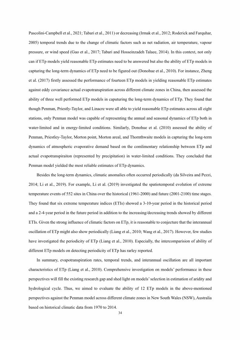
34

Pascolini-Campbell et al., 2021; Tabari et al., 2011) or decreasing (Irmak et al., 2012; Roderick and Farquhar,

2005) temporal trends due to the change of climatic factors such as net radiation, air temperature, vapour

pressure, or wind speed (Guo et al., 2017; Tabari and Hosseinzadeh Talaee, 2014). In this context, not only

can if ETp models yield reasonable ETp estimates need to be answered but also the ability of ETp models in

capturing the long-term dynamics of ETp need to be figured out (Donohue et al., 2010). For instance, Zheng

et al. (2017) firstly assessed the performance of fourteen ETp models in yielding reasonable ETp estimates

against eddy covariance actual evapotranspiration across different climate zones in China, then assessed the

ability of three well performed ETp models in caputuring the long-term dynamics of ETp. They found that

though Penman, Priestly-Taylor, and Linacre were all able to yield reasonable ETp estimates across all eight

stations, only Penman model was capable of representing the annual and seasonal dynamics of ETp both in

water-limited and in energy-limited conditions. Similarly, Donohue et al. (2010) assessed the ability of

Penman, Priestley-Taylor, Morton point, Morton areal, and Thornthwaite models in capturing the long-term

dynamics of atmospheric evaporative demand based on the comlimentary relationship between ETp and

actual evapotranspiraiton (represented by precipitation) in water-limited conditions. They concluded that

Penman model yielded the most reliable estimates of ETp dynamics.

Besides the long-term dynamics, climatic anomalies often occurred periodically (da Silveira and Pezzi,

2014; Li et al., 2019). For example, Li et al. (2019) investigated the spatiotemporal evolution of extreme

temperature events of 552 sites in China over the historical (1961-2000) and future (2001-2100) time stages.

They found that six extreme temperature indices (ETIs) showed a 3-10-year period in the historical period

and a 2-4-year period in the future period in addition to the increasing/decreasing trends showed by different

ETIs. Given the strong influence of climatic factors on ETp, it is reasonable to conjecture that the interannual

oscillation of ETp might also show periodically (Liang et al., 2010; Wang et al., 2017). However, few studies

have investigated the periodicity of ETp (Liang et al., 2010). Especially, the intercomparision of ability of

different ETp models on detecting periodicity of ETp has rarley reported.

In summary, evapotranspiration rates, temporal trends, and interannual oscillation are all important

characteristics of ETp (Liang et al., 2010). Comprehensive investigation on models’ performance in these

perspectives will fill the existing research gap and shed light on models’ selection in estimation of aridity and

hydrological cycle. Thus, we aimed to evaluate the ability of 12 ETp models in the above-mentioned

perspectives against the Penman model across different climate zones in New South Wales (NSW), Australia

based on historical climatic data from 1970 to 2014.

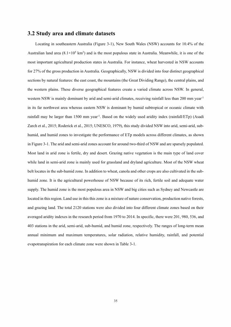
35

3.2 Study area and climate datasets

Locating in southeastern Australia (Figure 3-1), New South Wales (NSW) accounts for 10.4% of the

Australian land area (8.1×105 km2) and is the most populous state in Australia. Meanwhile, it is one of the

most important agricultural production states in Australia. For instance, wheat harvested in NSW accounts

for 27% of the gross production in Australia. Geographically, NSW is divided into four distinct geographical

sections by natural features: the east coast, the mountains (the Great Dividing Range), the central plains, and

the western plains. These diverse geographical features create a varied climate across NSW. In general,

western NSW is mainly dominant by arid and semi-arid climates, receiving rainfall less than 200 mm year-1

in its far northwest area whereas eastern NSW is dominant by humid subtropical or oceanic climate with

rainfall may be larger than 1500 mm year-1. Based on the widely used aridity index (rainfall/ETp) (Asadi

Zarch et al., 2015; Roderick et al., 2015; UNESCO, 1979), this study divided NSW into arid, semi-arid, sub-

humid, and humid zones to investigate the performance of ETp models across different climates, as shown

in Figure 3-1. The arid and semi-arid zones account for around two-third of NSW and are sparsely populated.

Most land in arid zone is fertile, dry and desert. Grazing native vegetation is the main type of land cover

while land in semi-arid zone is mainly used for grassland and dryland agriculture. Most of the NSW wheat

belt locates in the sub-humid zone. In addition to wheat, canola and other crops are also cultivated in the sub-

humid zone. It is the agricultural powerhouse of NSW because of its rich, fertile soil and adequate water

supply. The humid zone is the most populous area in NSW and big cities such as Sydney and Newcastle are

located in this region. Land use in this this zone is a mixture of nature conservation, production native forests,

and grazing land. The total 2120 stations were also divided into four different climate zones based on their

averaged aridity indexes in the research period from 1970 to 2014. In specific, there were 201, 980, 536, and

403 stations in the arid, semi-arid, sub-humid, and humid zone, respectively. The ranges of long-term mean

annual minimum and maximum temperatures, solar radiation, relative humidity, rainfall, and potential

evapotranspiration for each climate zone were shown in Table 3-1.

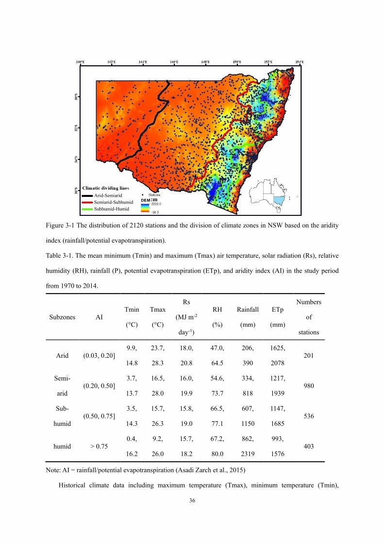
36

Figure 3-1 The distribution of 2120 stations and the division of climate zones in NSW based on the aridity

index (rainfall/potential evapotranspiration).

Table 3-1. The mean minimum (Tmin) and maximum (Tmax) air temperature, solar radiation (Rs), relative

humidity (RH), rainfall (P), potential evapotranspiration (ETp), and aridity index (AI) in the study period

from 1970 to 2014.

Subzones AI Tmin

(°C)

Tmax

(°C)

Rs

(MJ m-2

day-1)

RH

(%)

Rainfall

(mm)

ETp

(mm)

Numbers

of

stations

Arid (0.03, 0.20] 9.9,

14.8

23.7,

28.3

18.0,

20.8

47.0,

64.5

206,

390

1625,

2078 201

Semi-

arid (0.20, 0.50]

3.7,

13.7

16.5,

28.0

16.0,

19.9

54.6,

73.7

334,

818

1217,

1939 980

Sub-

humid (0.50, 0.75]

3.5,

14.3

15.7,

26.3

15.8,

19.0

66.5,

77.1

607,

1150

1147,

1685 536

humid > 0.75 0.4,

16.2

9.2,

26.0

15.7,

18.2

67.2,

80.0

862,

2319

993,

1576 403

Note: AI = rainfall/potential evapotranspiration (Asadi Zarch et al., 2015)

Historical climate data including maximum temperature (Tmax), minimum temperature (Tmin),

Arid-Semiarid Semiarid-Subhumid Subhumid-Humid

:m

37

maximum relative humidity (RHmax), minimum relative humidity (RHmin), rainfall (P), and solar radiation

(Rs) for 2120 stations across NSW were obtained from the Scientific Information for Land Owners (SILO)

patched point dataset (https://www.longpaddock.qld.gov.au/silo/datadrill/index.php). The patched data were

generated based on available ground-based observational data with spatial interpolation method at a spatial

resolution of 0.05° grid (Jeffrey et al., 2001). Thin plate smoothing spline method was used to construct the

missing daily climate variables while ordinary kriging method was used to construct missing daily rainfall.

More details about this dataset could be referred to Jeffrey et al. (2001). After its publication, the dataset has

been widely used in drought assessment, crop yield simulation, and other climate-related research in Australia

(Ahooghalandari et al., 2016; Howden et al., 2014; Karine et al., 2013).

The measured wind speed data for most stations was not available. In this case, this study adopted the

recommended 2 m s-1 by FAO56 as the surrogate wind speed (Allen et al., 1998; Tomas-Burguera et al.,

2017). The recommended 2m s-1 has been widely used in areas where observed wind speed is not available

and is reported that wind speed has relatively small influence on ETp estimates except for arid and windy

regions (Popova et al., 2006; Sentelhas et al., 2010). The reasonability of adopting the 2 m s-1 instead of

observed wind speed was also tested in this study based on eight stations which were Tibooburra and

Wilcannia from arid zone; Cobar and Gunnedah from semi-arid zone; Murrurundi and Paterson from sub-

humid zone; and Sydney and Coffs Harbour from humid zone. For these stations, the measured wind speed

was obtained from the Bureau of Meteorology (http://www.bom.gov.au/). Figure 3-2 showed the scatter plot

between ETp estimated with observed wind speed and ETp estimated with the recommended 2 m s-1 by

models used in this study which were based on wind speed. It suggested the R2 ranged from 0.69 to 0.97,

implying the reasonability of use of recommended wind speed.

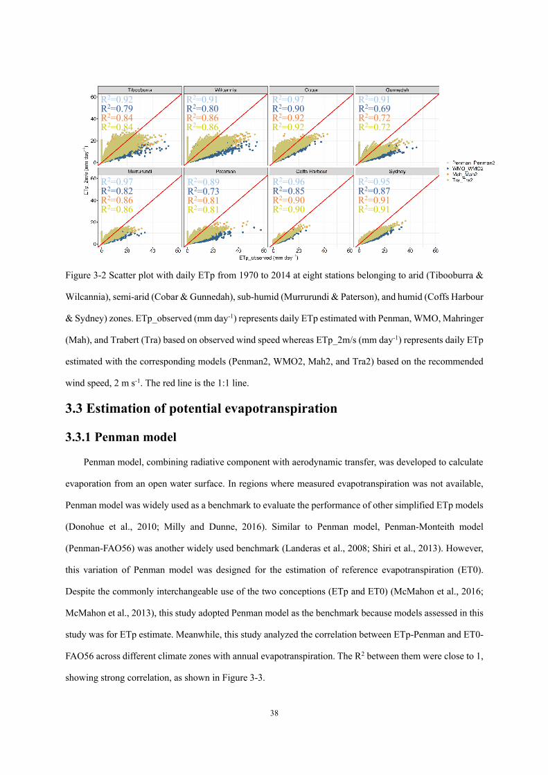
38

Figure 3-2 Scatter plot with daily ETp from 1970 to 2014 at eight stations belonging to arid (Tibooburra &

Wilcannia), semi-arid (Cobar & Gunnedah), sub-humid (Murrurundi & Paterson), and humid (Coffs Harbour

& Sydney) zones. ETp_observed (mm day-1) represents daily ETp estimated with Penman, WMO, Mahringer

(Mah), and Trabert (Tra) based on observed wind speed whereas ETp_2m/s (mm day-1) represents daily ETp

estimated with the corresponding models (Penman2, WMO2, Mah2, and Tra2) based on the recommended

wind speed, 2 m s-1. The red line is the 1:1 line.

3.3 Estimation of potential evapotranspiration

3.3.1 Penman model

Penman model, combining radiative component with aerodynamic transfer, was developed to calculate

evaporation from an open water surface. In regions where measured evapotranspiration was not available,

Penman model was widely used as a benchmark to evaluate the performance of other simplified ETp models

(Donohue et al., 2010; Milly and Dunne, 2016). Similar to Penman model, Penman-Monteith model

(Penman-FAO56) was another widely used benchmark (Landeras et al., 2008; Shiri et al., 2013). However,

this variation of Penman model was designed for the estimation of reference evapotranspiration (ET0).

Despite the commonly interchangeable use of the two conceptions (ETp and ET0) (McMahon et al., 2016;

McMahon et al., 2013), this study adopted Penman model as the benchmark because models assessed in this

study was for ETp estimate. Meanwhile, this study analyzed the correlation between ETp-Penman and ET0-

FAO56 across different climate zones with annual evapotranspiration. The R2 between them were close to 1,

showing strong correlation, as shown in Figure 3-3.

R2=0.92 R2=0.79 R2=0.84 R2=0.84

R2=0.91 R2=0.80 R2=0.86 R2=0.86

R2=0.97 R2=0.90 R2=0.92 R2=0.92

R2=0.91 R2=0.69 R2=0.72 R2=0.72

R2=0.97 R2=0.82 R2=0.86 R2=0.86

R2=0.89 R2=0.73 R2=0.81 R2=0.81

R2=0.96 R2=0.85 R2=0.90 R2=0.90

R2=0.95 R2=0.87 R2=0.91 R2=0.91

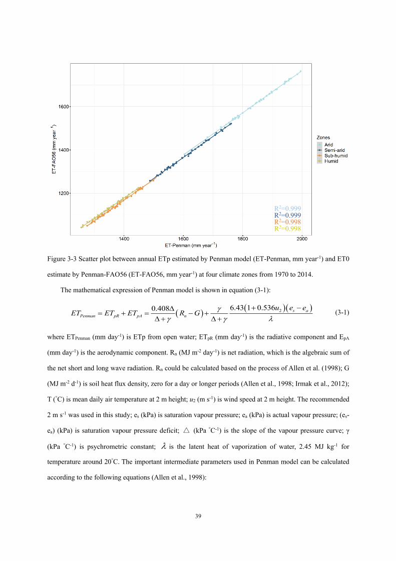
39

Figure 3-3 Scatter plot between annual ETp estimated by Penman model (ET-Penman, mm year-1) and ET0

estimate by Penman-FAO56 (ET-FAO56, mm year-1) at four climate zones from 1970 to 2014.

The mathematical expression of Penman model is shown in equation (3-1):

( )( )( )26.43 1 0.5360.408 s a

Penman pR pA n

u e eET ET ET R G

+ −= + = − +

+ + (3-1)

where ETPenman (mm day-1) is ETp from open water; ETpR (mm day-1) is the radiative component and EpA

(mm day-1) is the aerodynamic component. Rn (MJ m-2 day-1) is net radiation, which is the algebraic sum of

the net short and long wave radiation. Rn could be calculated based on the process of Allen et al. (1998); G

(MJ m-2 d-1) is soil heat flux density, zero for a day or longer periods (Allen et al., 1998; Irmak et al., 2012);

T (°C) is mean daily air temperature at 2 m height; u2 (m s-1) is wind speed at 2 m height. The recommended

2 m s-1 was used in this study; es (kPa) is saturation vapour pressure; ea (kPa) is actual vapour pressure; (es-

ea) (kPa) is saturation vapour pressure deficit; △ (kPa °C-1) is the slope of the vapour pressure curve; γ

(kPa °C-1) is psychrometric constant; is the latent heat of vaporization of water, 2.45 MJ kg-1 for

temperature around 20°C. The important intermediate parameters used in Penman model can be calculated

according to the following equations (Allen et al., 1998):

R2=0.999 R2=0.999 R2=0.998 R2=0.998

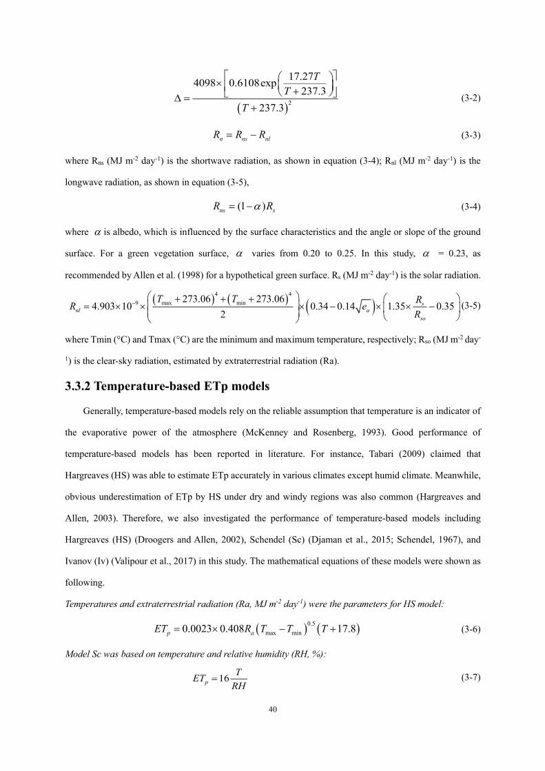
40

( )2

17.274098 0.6108exp237.3

237.3

TT

T

+ =

+ (3-2)

n ns nlR R R= − (3-3)

where Rns (MJ m-2 day-1) is the shortwave radiation, as shown in equation (3-4); Rnl (MJ m-2 day-1) is the

longwave radiation, as shown in equation (3-5),

(1 )ns sR R= − (3-4)

where is albedo, which is influenced by the surface characteristics and the angle or slope of the ground

surface. For a green vegetation surface, varies from 0.20 to 0.25. In this study, = 0.23, as

recommended by Allen et al. (1998) for a hypothetical green surface. Rs (MJ m-2 day-1) is the solar radiation.

( ) ( )( )

4 4max min9 273.06 273.06

4.903 10 0.34 0.14 1.35 0.352

snl a

so

T T RR eR

− + + +

= − −

(3-5)

where Tmin (°C) and Tmax (°C) are the minimum and maximum temperature, respectively; Rso (MJ m-2 day-

1) is the clear-sky radiation, estimated by extraterrestrial radiation (Ra).

3.3.2 Temperature-based ETp models

Generally, temperature-based models rely on the reliable assumption that temperature is an indicator of

the evaporative power of the atmosphere (McKenney and Rosenberg, 1993). Good performance of

temperature-based models has been reported in literature. For instance, Tabari (2009) claimed that

Hargreaves (HS) was able to estimate ETp accurately in various climates except humid climate. Meanwhile,

obvious underestimation of ETp by HS under dry and windy regions was also common (Hargreaves and

Allen, 2003). Therefore, we also investigated the performance of temperature-based models including

Hargreaves (HS) (Droogers and Allen, 2002), Schendel (Sc) (Djaman et al., 2015; Schendel, 1967), and

Ivanov (Iv) (Valipour et al., 2017) in this study. The mathematical equations of these models were shown as

following.

Temperatures and extraterrestrial radiation (Ra, MJ m-2 day-1) were the parameters for HS model:

( ) ( )0.5

max min0.0023 0.408 17.8p aET R T T T= − + (3-6)

Model Sc was based on temperature and relative humidity (RH, %):

16pTET

RH= (3-7)

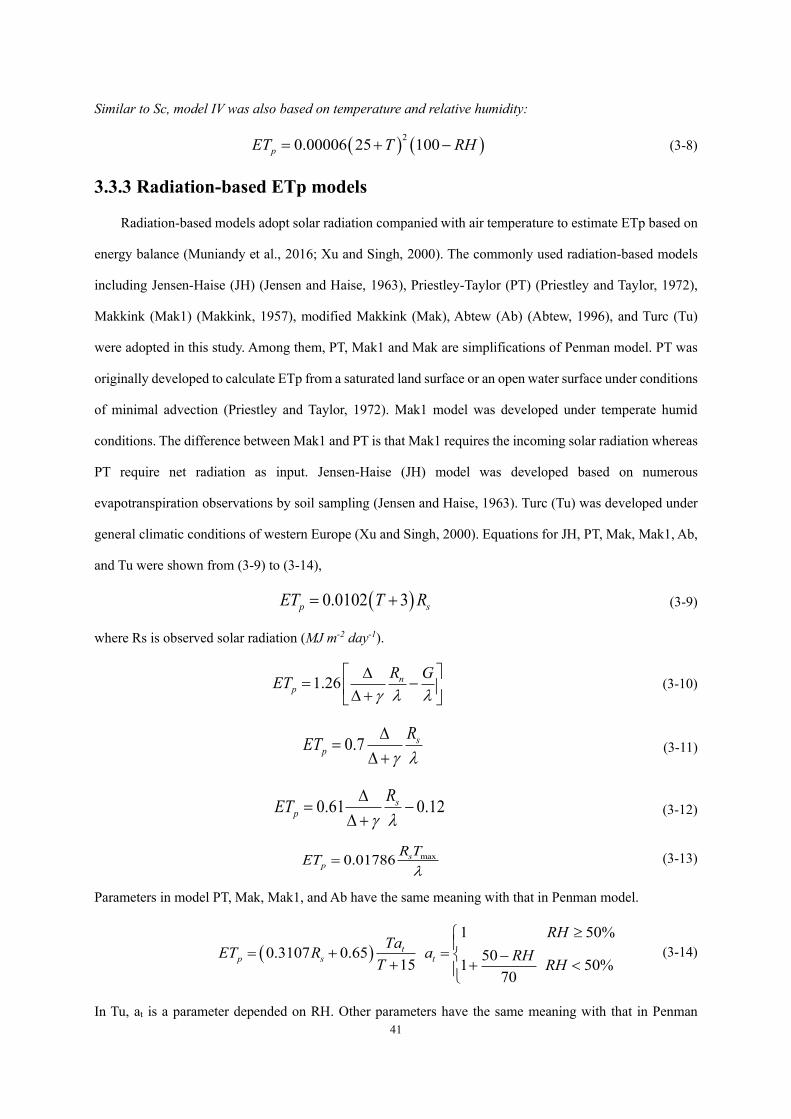
41

Similar to Sc, model IV was also based on temperature and relative humidity:

( ) ( )20.00006 25 100pET T RH= + − (3-8)

3.3.3 Radiation-based ETp models

Radiation-based models adopt solar radiation companied with air temperature to estimate ETp based on

energy balance (Muniandy et al., 2016; Xu and Singh, 2000). The commonly used radiation-based models

including Jensen-Haise (JH) (Jensen and Haise, 1963), Priestley-Taylor (PT) (Priestley and Taylor, 1972),

Makkink (Mak1) (Makkink, 1957), modified Makkink (Mak), Abtew (Ab) (Abtew, 1996), and Turc (Tu)

were adopted in this study. Among them, PT, Mak1 and Mak are simplifications of Penman model. PT was

originally developed to calculate ETp from a saturated land surface or an open water surface under conditions

of minimal advection (Priestley and Taylor, 1972). Mak1 model was developed under temperate humid

conditions. The difference between Mak1 and PT is that Mak1 requires the incoming solar radiation whereas

PT require net radiation as input. Jensen-Haise (JH) model was developed based on numerous

evapotranspiration observations by soil sampling (Jensen and Haise, 1963). Turc (Tu) was developed under

general climatic conditions of western Europe (Xu and Singh, 2000). Equations for JH, PT, Mak, Mak1, Ab,

and Tu were shown from (3-9) to (3-14),

( )0.0102 3p sET T R= + (3-9)

where Rs is observed solar radiation (MJ m-2 day-1).

1.26 np

R GET

= −

+ (3-10)

0.7 sp

RET

=

+ (3-11)

0.61 0.12sp

RET

= −

+ (3-12)

max0.01786 sp

R TET

= (3-13)

Parameters in model PT, Mak, Mak1, and Ab have the same meaning with that in Penman model.

( )1 50%

0.3107 0.65 5015 1 50%70

tp s t

RHTaET R a RHT RH

= + = −+ +

(3-14)

In Tu, at is a parameter depended on RH. Other parameters have the same meaning with that in Penman

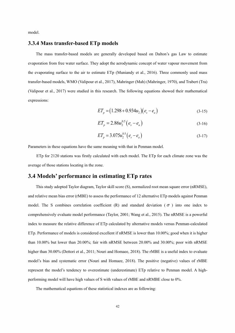
42

model.

3.3.4 Mass transfer-based ETp models

The mass transfer-based models are generally developed based on Dalton’s gas Law to estimate

evaporation from free water surface. They adopt the aerodynamic concept of water vapour movement from

the evaporating surface to the air to estimate ETp (Muniandy et al., 2016). Three commonly used mass

transfer-based models, WMO (Valipour et al., 2017), Mahringer (Mah) (Mahringer, 1970), and Trabert (Tra)

(Valipour et al., 2017) were studied in this research. The following equations showed their mathematical

expressions:

( )( )21.298 0.934p s aET u e e= + − (3-15)

( )0.522.86p s aET u e e= − (3-16)

( )0.523.075p s aET u e e= − (3-17)

Parameters in these equations have the same meaning with that in Penman model.

ETp for 2120 stations was firstly calculated with each model. The ETp for each climate zone was the

average of those stations locating in the zone.

3.4 Models’ performance in estimating ETp rates

This study adopted Taylor diagram, Taylor skill score (S), normalized root mean square error (nRMSE),

and relative mean bias error (rMBE) to assess the performance of 12 alternative ETp models against Penman

model. The S combines correlation coefficient (R) and standard deviation ( ) into one index to

comprehensively evaluate model performance (Taylor, 2001; Wang et al., 2015). The nRMSE is a powerful

index to measure the relative difference of ETp calculated by alternative models versus Penman-calculated

ETp. Performance of models is considered excellent if nRMSE is lower than 10.00%; good when it is higher

than 10.00% but lower than 20.00%; fair with nRMSE between 20.00% and 30.00%; poor with nRMSE

higher than 30.00% (Dettori et al., 2011; Nouri and Homaee, 2018). The rMBE is a useful index to evaluate

model’s bias and systematic error (Nouri and Homaee, 2018). The positive (negative) values of rMBE

represent the model’s tendency to overestimate (underestimate) ETp relative to Penman model. A high-

performing model will have high values of S with values of rMBE and nRMBE close to 0%.

The mathematical equations of these statistical indexes are as following:

43

( )

( )

2

22

0

4 1(3-18)

1PenmanM

Penman M

RS

R

+=

+ +

where S is the Taylor skill score; R is the correlation coefficient between an alternative model and Penman

model; R0 is the maximum correlation coefficient attainable (0.999 is used in this study). M and Penman

are the standard deviations of ETp for an alternative model and Penamn model, respectively;

( )2

, ,1

100 1 (3-19)n

M i Penman iiPenman

nRMSE ET ETnET =

= −

( ), ,1

100 1 (3-20)n

M i Penman iiPenman

rMBE ET ETnET =

= −

where ETM,i and ETPenman,i are ETp calculated with an alternative model and Penman model, respectively.

PenmanET is the average Penman-calculated ETp and n is the number of the sample.

3.5 Models’ ability in capturing ETp dynamics and periodic oscillations

The relationship between ETp and actual evapotranspiration is complementary under water-limited

condition and proportional under energy-limited condition (Yang et al., 2006). In specific, actual

evapotranspiration will increase when precipitation increases under water-limited condition whereas ETp

will decrease as a result of the decreases in solar radiation and air temperature, and increases in air humidity

(Zheng et al., 2017). Referred to Donohue et al. (2010), they compared the trends of ETp estimated by five

different models against the trends in precipitation to assess ETp model’s ability in representing the long-

term dynamics of evaporative demand. In other words, models which show inverse trends against

precipitation are reliable in capturing the dynamics of evaporative demand under water-limited conditions.

This study followed the method and compared the trends of ETp and precipitation tested by Mann-Kendall

to assess models’ ability in capturing the dynamics of evaporative demand.

The Mann-Kendall (M-K) test is highly recommended by the World Meteorological Organization to

identify trends in hydro-meteorological time series (Han et al., 2018). Under a changing climate, this method

has also been widely used to determine temporal trends in climatic variables and ETp series (Lin et al., 2018;

Lv et al., 2016). The standardized test statistic, Z, is provided in M-K test to indicate if the temporal trend of

a variable is significant. At the 95% confidence level, temporal trends are significant when ｜Z｜> 1.96;

time series trends are significant at 99% confidence level when｜Z｜> 2.58. A positive Z-value shows an

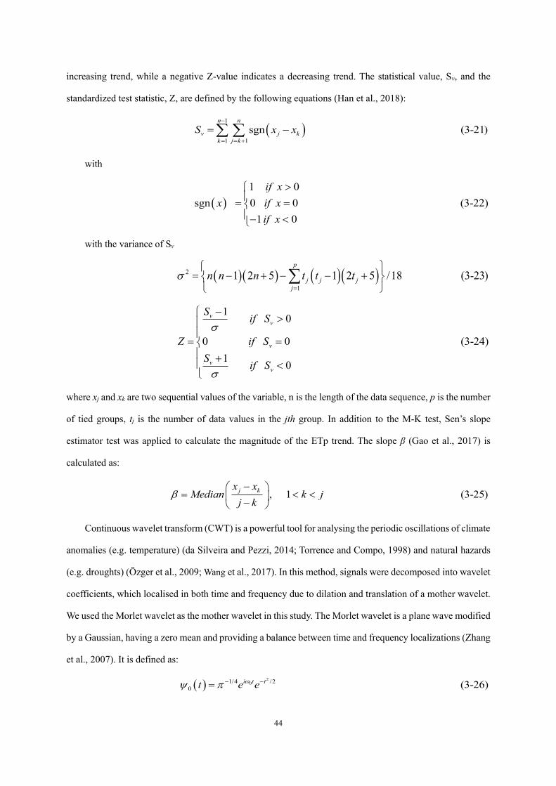
44

increasing trend, while a negative Z-value indicates a decreasing trend. The statistical value, Sv, and the

standardized test statistic, Z, are defined by the following equations (Han et al., 2018):

( )1

1 1sgn (3-21)

n n

v j kk j k

S x x−

= = +

= −

with

( )

1 0sgn 0 0 (3-22)

1 0

if xx if x

if x

= =−

with the variance of Sv

( )( ) ( )( )2

11 2 5 1 2 5 /18 (3-23)

p

j j jj

n n n t t t=

= − + − − +

1 0

0 0 (3-24)1 0

vv

v

vv

S if S

Z if SS if S

−

= = +

where xj and xk are two sequential values of the variable, n is the length of the data sequence, p is the number

of tied groups, tj is the number of data values in the jth group. In addition to the M-K test, Sen’s slope

estimator test was applied to calculate the magnitude of the ETp trend. The slope β (Gao et al., 2017) is

calculated as:

, 1 (3-25)j kx xMedian k j

j k

− =

−

Continuous wavelet transform (CWT) is a powerful tool for analysing the periodic oscillations of climate

anomalies (e.g. temperature) (da Silveira and Pezzi, 2014; Torrence and Compo, 1998) and natural hazards

(e.g. droughts) (Özger et al., 2009; Wang et al., 2017). In this method, signals were decomposed into wavelet

coefficients, which localised in both time and frequency due to dilation and translation of a mother wavelet.

We used the Morlet wavelet as the mother wavelet in this study. The Morlet wavelet is a plane wave modified

by a Gaussian, having a zero mean and providing a balance between time and frequency localizations (Zhang

et al., 2007). It is defined as:

( )2

01/4 /20 (3-26)i t tt e e − −=

45

where , the dimensionless angular frequency, was set to 6 to render the Morlet wavelet analytical (Farge,

1992).

3.6 Results

3.6.1 Performance of models in estimating ETp rates

Generally, models with higher S were also marked with lower nRMSE and lower absolute rMBE

independent of time scale (daily or seasonal). However, significant differences were found in S, nRMSE, and

rMBE among models both at daily and seasonal scales. Figure 3-4 showed that models generally achieved S

larger than 0.60 at daily scale. The difference of S among models was largest in arid and humid zones than

that in semi-arid and sub-humid zones. In addition, compared with radiation-based models, temperature-

based and mass transfer-based models except HS generally showed weaker correlation with Penman model.

Take humid zone as an example, the correlation coefficients of temperature-based and mass transfer-based

models were around 0.80 whereas the coefficients for radiation-based models were ranging from 0.97 to 0.99.

0

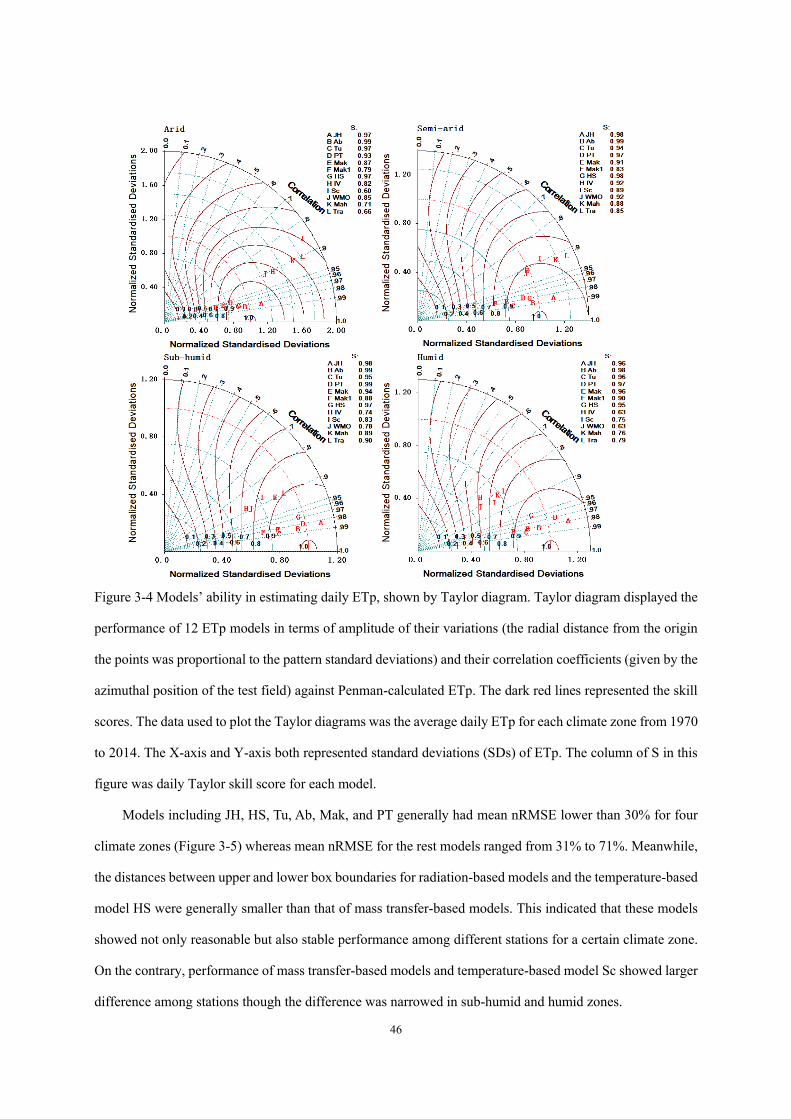
46

Figure 3-4 Models’ ability in estimating daily ETp, shown by Taylor diagram. Taylor diagram displayed the

performance of 12 ETp models in terms of amplitude of their variations (the radial distance from the origin

the points was proportional to the pattern standard deviations) and their correlation coefficients (given by the

azimuthal position of the test field) against Penman-calculated ETp. The dark red lines represented the skill

scores. The data used to plot the Taylor diagrams was the average daily ETp for each climate zone from 1970

to 2014. The X-axis and Y-axis both represented standard deviations (SDs) of ETp. The column of S in this

figure was daily Taylor skill score for each model.

Models including JH, HS, Tu, Ab, Mak, and PT generally had mean nRMSE lower than 30% for four

climate zones (Figure 3-5) whereas mean nRMSE for the rest models ranged from 31% to 71%. Meanwhile,

the distances between upper and lower box boundaries for radiation-based models and the temperature-based

model HS were generally smaller than that of mass transfer-based models. This indicated that these models

showed not only reasonable but also stable performance among different stations for a certain climate zone.

On the contrary, performance of mass transfer-based models and temperature-based model Sc showed larger

difference among stations though the difference was narrowed in sub-humid and humid zones.

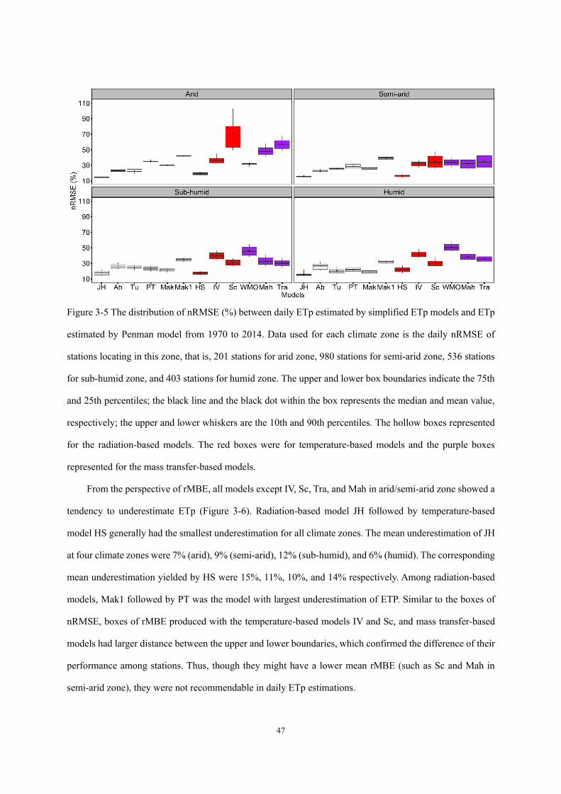
47

Figure 3-5 The distribution of nRMSE (%) between daily ETp estimated by simplified ETp models and ETp

estimated by Penman model from 1970 to 2014. Data used for each climate zone is the daily nRMSE of

stations locating in this zone, that is, 201 stations for arid zone, 980 stations for semi-arid zone, 536 stations

for sub-humid zone, and 403 stations for humid zone. The upper and lower box boundaries indicate the 75th

and 25th percentiles; the black line and the black dot within the box represents the median and mean value,

respectively; the upper and lower whiskers are the 10th and 90th percentiles. The hollow boxes represented

for the radiation-based models. The red boxes were for temperature-based models and the purple boxes

represented for the mass transfer-based models.

From the perspective of rMBE, all models except IV, Sc, Tra, and Mah in arid/semi-arid zone showed a

tendency to underestimate ETp (Figure 3-6). Radiation-based model JH followed by temperature-based

model HS generally had the smallest underestimation for all climate zones. The mean underestimation of JH

at four climate zones were 7% (arid), 9% (semi-arid), 12% (sub-humid), and 6% (humid). The corresponding

mean underestimation yielded by HS were 15%, 11%, 10%, and 14% respectively. Among radiation-based

models, Mak1 followed by PT was the model with largest underestimation of ETP. Similar to the boxes of

nRMSE, boxes of rMBE produced with the temperature-based models IV and Sc, and mass transfer-based

models had larger distance between the upper and lower boundaries, which confirmed the difference of their

performance among stations. Thus, though they might have a lower mean rMBE (such as Sc and Mah in

semi-arid zone), they were not recommendable in daily ETp estimations.

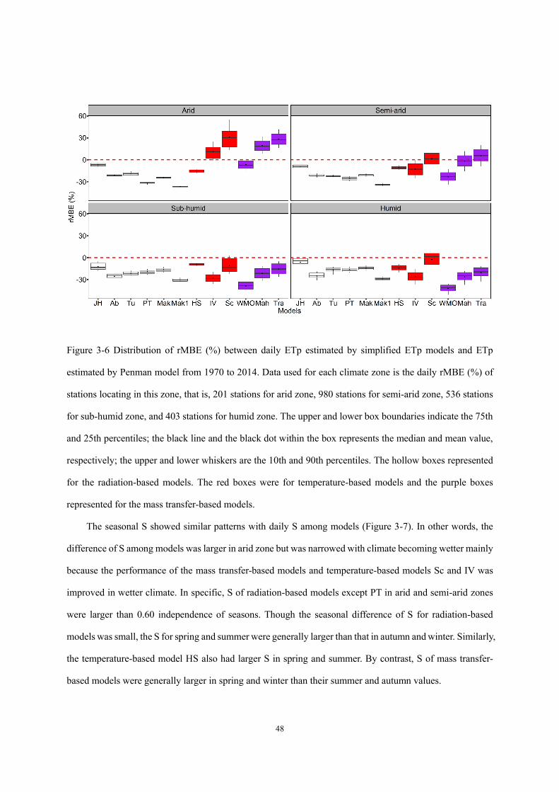
48

Figure 3-6 Distribution of rMBE (%) between daily ETp estimated by simplified ETp models and ETp

estimated by Penman model from 1970 to 2014. Data used for each climate zone is the daily rMBE (%) of

stations locating in this zone, that is, 201 stations for arid zone, 980 stations for semi-arid zone, 536 stations

for sub-humid zone, and 403 stations for humid zone. The upper and lower box boundaries indicate the 75th

and 25th percentiles; the black line and the black dot within the box represents the median and mean value,

respectively; the upper and lower whiskers are the 10th and 90th percentiles. The hollow boxes represented

for the radiation-based models. The red boxes were for temperature-based models and the purple boxes

represented for the mass transfer-based models.

The seasonal S showed similar patterns with daily S among models (Figure 3-7). In other words, the

difference of S among models was larger in arid zone but was narrowed with climate becoming wetter mainly

because the performance of the mass transfer-based models and temperature-based models Sc and IV was

improved in wetter climate. In specific, S of radiation-based models except PT in arid and semi-arid zones

were larger than 0.60 independence of seasons. Though the seasonal difference of S for radiation-based

models was small, the S for spring and summer were generally larger than that in autumn and winter. Similarly,

the temperature-based model HS also had larger S in spring and summer. By contrast, S of mass transfer-

based models were generally larger in spring and winter than their summer and autumn values.

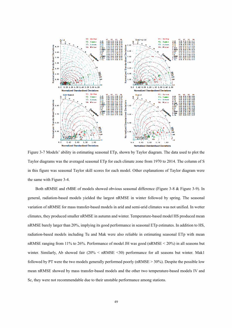
49

Figure 3-7 Models’ ability in estimating seasonal ETp, shown by Taylor diagram. The data used to plot the

Taylor diagrams was the averaged seasonal ETp for each climate zone from 1970 to 2014. The column of S

in this figure was seasonal Taylor skill scores for each model. Other explanations of Taylor diagram were

the same with Figure 3-4.

Both nRMSE and rMBE of models showed obvious seasonal difference (Figure 3-8 & Figure 3-9). In

general, radiation-based models yielded the largest nRMSE in winter followed by spring. The seasonal

variation of nRMSE for mass transfer-based models in arid and semi-arid climates was not unified. In wetter

climates, they produced smaller nRMSE in autumn and winter. Temperature-based model HS produced mean

nRMSE barely larger than 20%, implying its good performance in seasonal ETp estimates. In addition to HS,

radiation-based models including Tu and Mak were also reliable in estimating seasonal ETp with mean

nRMSE ranging from 11% to 26%. Performance of model JH was good (nRMSE < 20%) in all seasons but

winter. Similarly, Ab showed fair (20% < nRMSE <30) performance for all seasons but winter. Mak1

followed by PT were the two models generally performed poorly (nRMSE > 30%). Despite the possible low

mean nRMSE showed by mass transfer-based models and the other two temperature-based models IV and

Sc, they were not recommendable due to their unstable performance among stations.

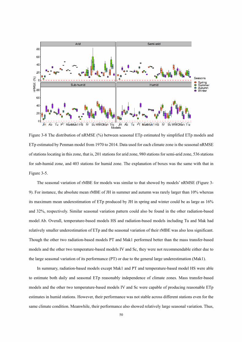
50

Figure 3-8 The distribution of nRMSE (%) between seasonal ETp estimated by simplified ETp models and

ETp estimated by Penman model from 1970 to 2014. Data used for each climate zone is the seasonal nRMSE

of stations locating in this zone, that is, 201 stations for arid zone, 980 stations for semi-arid zone, 536 stations

for sub-humid zone, and 403 stations for humid zone. The explanation of boxes was the same with that in

Figure 3-5.

The seasonal variation of rMBE for models was similar to that showed by models’ nRMSE (Figure 3-

9). For instance, the absolute mean rMBE of JH in summer and autumn was rarely larger than 10% whereas

its maximum mean underestimation of ETp produced by JH in spring and winter could be as large as 16%

and 32%, respectively. Similar seasonal variation pattern could also be found in the other radiation-based

model Ab. Overall, temperature-based models HS and radiation-based models including Tu and Mak had

relatively smaller underestimation of ETp and the seasonal variation of their rMBE was also less significant.

Though the other two radiation-based models PT and Mak1 performed better than the mass transfer-based

models and the other two temperature-based models IV and Sc, they were not recommendable either due to

the large seasonal variation of its performance (PT) or due to the general large underestimation (Mak1).

In summary, radiation-based models except Mak1 and PT and temperature-based model HS were able

to estimate both daily and seasonal ETp reasonably independence of climate zones. Mass transfer-based

models and the other two temperature-based models IV and Sc were capable of producing reasonable ETp

estimates in humid stations. However, their performance was not stable across different stations even for the

same climate condition. Meanwhile, their performance also showed relatively large seasonal variation. Thus,

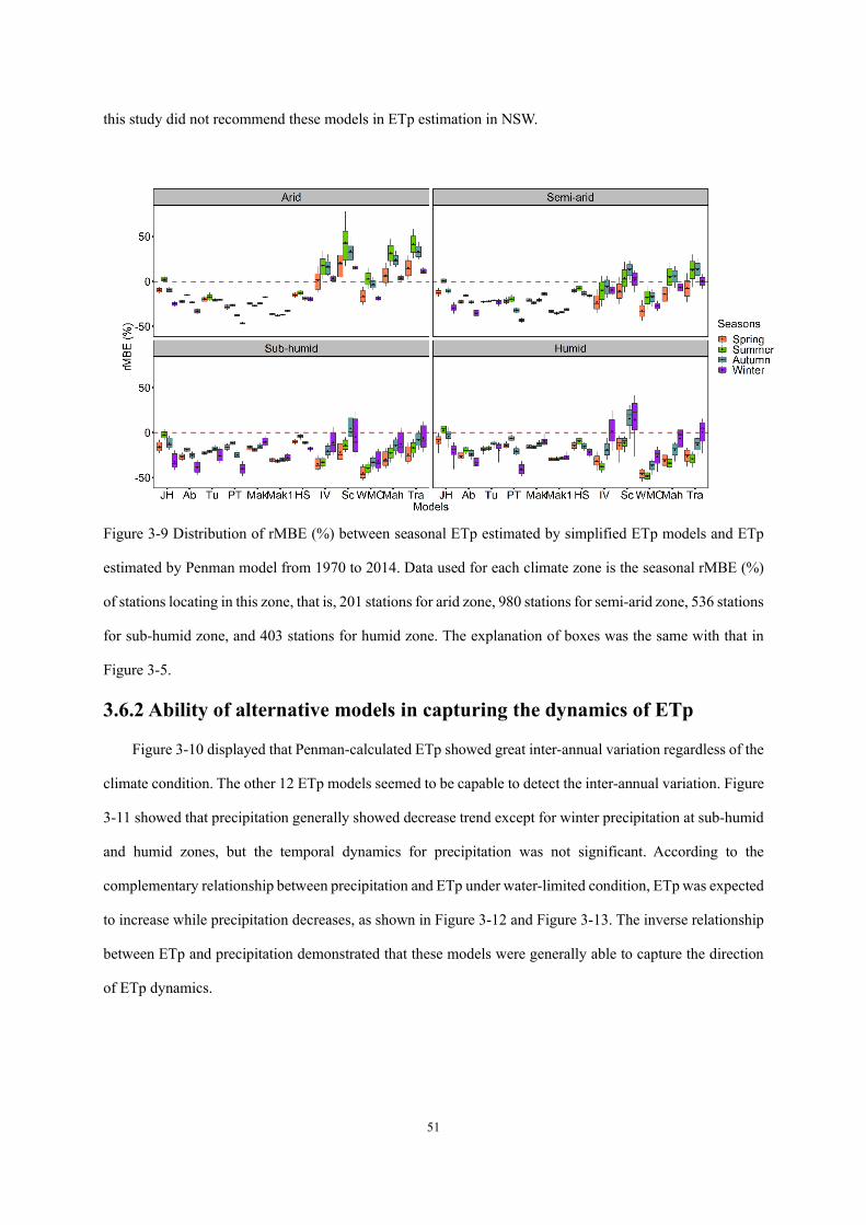
51

this study did not recommend these models in ETp estimation in NSW.

Figure 3-9 Distribution of rMBE (%) between seasonal ETp estimated by simplified ETp models and ETp

estimated by Penman model from 1970 to 2014. Data used for each climate zone is the seasonal rMBE (%)

of stations locating in this zone, that is, 201 stations for arid zone, 980 stations for semi-arid zone, 536 stations

for sub-humid zone, and 403 stations for humid zone. The explanation of boxes was the same with that in

Figure 3-5.

3.6.2 Ability of alternative models in capturing the dynamics of ETp

Figure 3-10 displayed that Penman-calculated ETp showed great inter-annual variation regardless of the

climate condition. The other 12 ETp models seemed to be capable to detect the inter-annual variation. Figure

3-11 showed that precipitation generally showed decrease trend except for winter precipitation at sub-humid

and humid zones, but the temporal dynamics for precipitation was not significant. According to the

complementary relationship between precipitation and ETp under water-limited condition, ETp was expected

to increase while precipitation decreases, as shown in Figure 3-12 and Figure 3-13. The inverse relationship

between ETp and precipitation demonstrated that these models were generally able to capture the direction

of ETp dynamics.

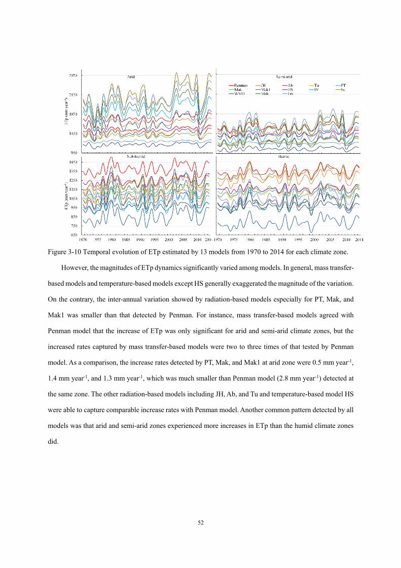
52

Figure 3-10 Temporal evolution of ETp estimated by 13 models from 1970 to 2014 for each climate zone.

However, the magnitudes of ETp dynamics significantly varied among models. In general, mass transfer-

based models and temperature-based models except HS generally exaggerated the magnitude of the variation.

On the contrary, the inter-annual variation showed by radiation-based models especially for PT, Mak, and

Mak1 was smaller than that detected by Penman. For instance, mass transfer-based models agreed with

Penman model that the increase of ETp was only significant for arid and semi-arid climate zones, but the

increased rates captured by mass transfer-based models were two to three times of that tested by Penman

model. As a comparison, the increase rates detected by PT, Mak, and Mak1 at arid zone were 0.5 mm year-1,

1.4 mm year-1, and 1.3 mm year-1, which was much smaller than Penman model (2.8 mm year-1) detected at

the same zone. The other radiation-based models including JH, Ab, and Tu and temperature-based model HS

were able to capture comparable increase rates with Penman model. Another common pattern detected by all

models was that arid and semi-arid zones experienced more increases in ETp than the humid climate zones

did.

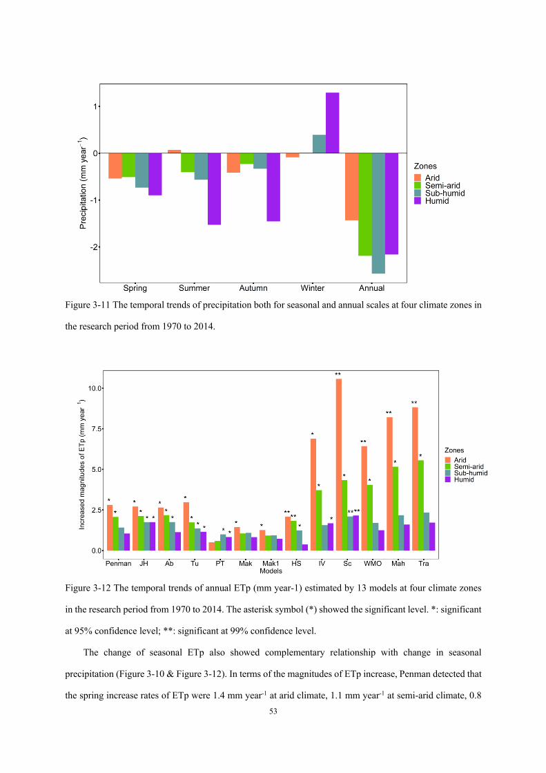
53

Figure 3-11 The temporal trends of precipitation both for seasonal and annual scales at four climate zones in

the research period from 1970 to 2014.

Figure 3-12 The temporal trends of annual ETp (mm year-1) estimated by 13 models at four climate zones

in the research period from 1970 to 2014. The asterisk symbol (*) showed the significant level. *: significant

at 95% confidence level; **: significant at 99% confidence level.

The change of seasonal ETp also showed complementary relationship with change in seasonal

precipitation (Figure 3-10 & Figure 3-12). In terms of the magnitudes of ETp increase, Penman detected that

the spring increase rates of ETp were 1.4 mm year-1 at arid climate, 1.1 mm year-1 at semi-arid climate, 0.8

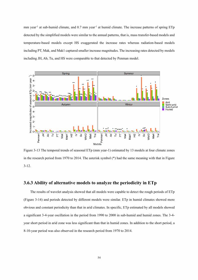
54

mm year-1 at sub-humid climate, and 0.7 mm year-1 at humid climate. The increase patterns of spring ETp

detected by the simplified models were similar to the annual patterns, that is, mass transfer-based models and

temperature-based models except HS exaggerated the increase rates whereas radiation-based models

including PT, Mak, and Mak1 captured smaller increase magnitudes. The increasing rates detected by models

including JH, Ab, Tu, and HS were comparable to that detected by Penman model.

Figure 3-13 The temporal trends of seasonal ETp (mm year-1) estimated by 13 models at four climate zones

in the research period from 1970 to 2014. The asterisk symbol (*) had the same meaning with that in Figure

3-12.

3.6.3 Ability of alternative models to analyze the periodicity in ETp

The results of wavelet analysis showed that all models were capable to detect the rough periods of ETp

(Figure 3-14) and periods detected by different models were similar. ETp in humid climates showed more

obvious and constant periodicity than that in arid climates. In specific, ETp estimated by all models showed

a significant 3-4-year oscillation in the period from 1990 to 2000 in sub-humid and humid zones. The 3-4-

year short period in arid zone was less significant than that in humid zones. In addition to the short period, a

8-10-year period was also observed in the research period from 1970 to 2014.

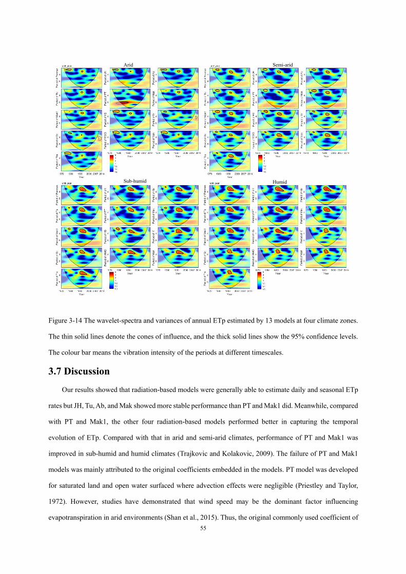
55

Figure 3-14 The wavelet-spectra and variances of annual ETp estimated by 13 models at four climate zones.

The thin solid lines denote the cones of influence, and the thick solid lines show the 95% confidence levels.

The colour bar means the vibration intensity of the periods at different timescales.

3.7 Discussion

Our results showed that radiation-based models were generally able to estimate daily and seasonal ETp

rates but JH, Tu, Ab, and Mak showed more stable performance than PT and Mak1 did. Meanwhile, compared

with PT and Mak1, the other four radiation-based models performed better in capturing the temporal

evolution of ETp. Compared with that in arid and semi-arid climates, performance of PT and Mak1 was

improved in sub-humid and humid climates (Trajkovic and Kolakovic, 2009). The failure of PT and Mak1

models was mainly attributed to the original coefficients embedded in the models. PT model was developed

for saturated land and open water surfaced where advection effects were negligible (Priestley and Taylor,

1972). However, studies have demonstrated that wind speed may be the dominant factor influencing

evapotranspiration in arid environments (Shan et al., 2015). Thus, the original commonly used coefficient of

Arid Semi-arid

Sub-humid Humid

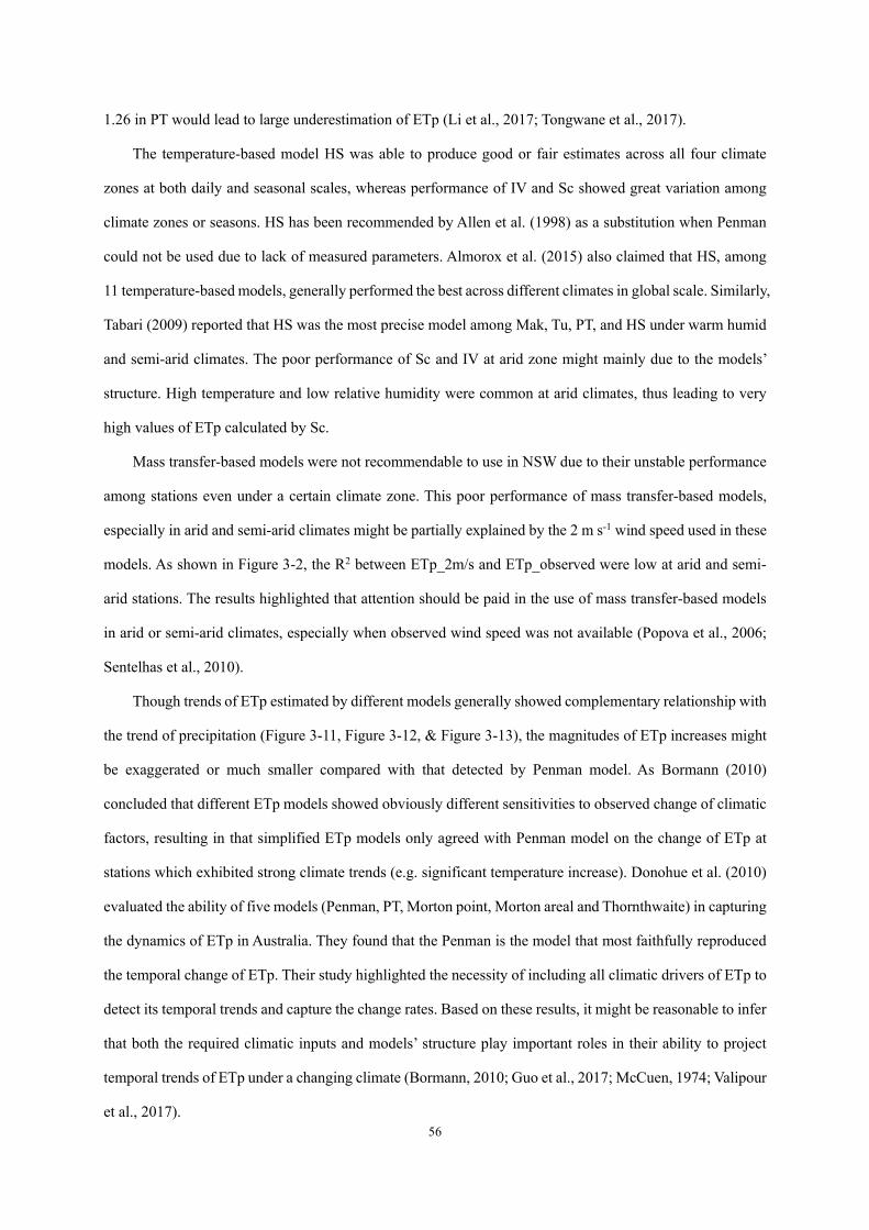
56

1.26 in PT would lead to large underestimation of ETp (Li et al., 2017; Tongwane et al., 2017).

The temperature-based model HS was able to produce good or fair estimates across all four climate

zones at both daily and seasonal scales, whereas performance of IV and Sc showed great variation among

climate zones or seasons. HS has been recommended by Allen et al. (1998) as a substitution when Penman

could not be used due to lack of measured parameters. Almorox et al. (2015) also claimed that HS, among

11 temperature-based models, generally performed the best across different climates in global scale. Similarly,

Tabari (2009) reported that HS was the most precise model among Mak, Tu, PT, and HS under warm humid

and semi-arid climates. The poor performance of Sc and IV at arid zone might mainly due to the models’

structure. High temperature and low relative humidity were common at arid climates, thus leading to very

high values of ETp calculated by Sc.

Mass transfer-based models were not recommendable to use in NSW due to their unstable performance

among stations even under a certain climate zone. This poor performance of mass transfer-based models,

especially in arid and semi-arid climates might be partially explained by the 2 m s-1 wind speed used in these

models. As shown in Figure 3-2, the R2 between ETp_2m/s and ETp_observed were low at arid and semi-

arid stations. The results highlighted that attention should be paid in the use of mass transfer-based models

in arid or semi-arid climates, especially when observed wind speed was not available (Popova et al., 2006;

Sentelhas et al., 2010).

Though trends of ETp estimated by different models generally showed complementary relationship with

the trend of precipitation (Figure 3-11, Figure 3-12, & Figure 3-13), the magnitudes of ETp increases might

be exaggerated or much smaller compared with that detected by Penman model. As Bormann (2010)

concluded that different ETp models showed obviously different sensitivities to observed change of climatic

factors, resulting in that simplified ETp models only agreed with Penman model on the change of ETp at

stations which exhibited strong climate trends (e.g. significant temperature increase). Donohue et al. (2010)

evaluated the ability of five models (Penman, PT, Morton point, Morton areal and Thornthwaite) in capturing

the dynamics of ETp in Australia. They found that the Penman is the model that most faithfully reproduced

the temporal change of ETp. Their study highlighted the necessity of including all climatic drivers of ETp to

detect its temporal trends and capture the change rates. Based on these results, it might be reasonable to infer

that both the required climatic inputs and models’ structure play important roles in their ability to project

temporal trends of ETp under a changing climate (Bormann, 2010; Guo et al., 2017; McCuen, 1974; Valipour

et al., 2017).

57

The comparison of models’ ability in detecting periodicity of ETp was rare in literature. According to

our study, we found that the studied models showed roughly equal ability in detecting the periodicity of ETp.

3-4-year and 8-10-year periodical oscillation of ETp have also been observed in this study, which was also

supported by other researchers. For instance, Wang et al. (2017) claimed that the periods of 2.4, 3.4, and 9.6

years of ETp existed in China from 1961 to 2013. They claimed that El Niño/Southern Oscillation (ENSO)

might be the climatic force of the oscillations of ETp (Wang et al., 2017). Similarly, we found that the low

peaks of ETp were corresponding to the classic La Niña years while the high peaks of ETp were

corresponding to the classic El Niño events occurred in Australia (BOM, 2012). When El Niño occurs it

generally results in less rainfall, higher temperature and reduced cloudiness, thus increasing ETp and actual

ET if water is available. At Taoer River basin of Northeast China, Liang et al. (2010) reported a 2-8 year

periods of ETp from 1961 to 2005. They argued that the periodicity of maximum temperature, mean air

temperature, relative humidity and solar radiation were main climate variables leading to the periodical

oscillation in evapotranspiration.

Models evaluated in this study were temperature-based, radiation-based, or mass transfer-based. Among

them, the use of some mass transfer-based models has been abandoned due to the great deviations in ETp

estimated by these models (Bormann, 2010; Xiang et al., 2020). Especially, temperature-based and radiation-

based models may be more feasible in ETp projection under future climate scenarios given the fact that the

projection of temperature and radiation is more reliable than that of wind speed and humidity (Guo et al.,

2017). Thus, based on findings in this study, radiation-based models including JH, Mak, and Ab, and

temperature-based models HS were recommended to project future ETp.

It is likely that a location-specific calibration might improve model performance (Cristea et al., 2013;

Shiri, 2017; Sumner and Jacobs, 2005; Xu and Singh, 2002). However, the readjustment of models’

coefficients could be site-specific (Ravazzani et al., 2012) and greatly depend on the study period (Raziei

and Pereira, 2013; Tabari and Talaee, 2011). In other words, the possibility of misleading to decision-makers

companies with the readjustment of original coefficients embedded in empirical modes (Nouri and Homaee,

2018). Thus, we only evaluated models’ performance based on the original coefficients.

3.8 Conclusions

The performance of 12 models in estimating ETp rates and capturing its temporal trends and interannual

oscillation were evaluated against Penman model at four different climate zones in NSW from 1970 to 2014.

58

This study showed that radiation-based models and temperature-based model HS exhibited acceptable and

stable performance in estimating both daily and seasonal ETp rates across all stations. Meanwhile, they

showed comparable ability against Penman model in detecting the periodical oscillation of ETp in the

research period. However, radiation-based models PT and Mak1 generally underestimated the increase rates

of ETp. Thus, this study recommended the use of JH, Tu, Ab, Mak, and HS to estimate ETp in NSW when

the whole set of climatic data was not available to use Penman model.

59

3.9 Reference Abtew, W., 1996. Evapotranspiration measurements and modeling for three wetland systems in south

florida. Jawra Journal of the American Water Resources Association, 32(3): 465-473.

Abtew, W., Melesse, A., 2012. Evaporation and evapotranspiration: measurements and estimations. Springer

Science & Business Media.

Ahooghalandari, M., Khiadani, M., Jahromi, M.E., 2016. Calibration of Valiantzas’ reference

evapotranspiration equations for the Pilbara region, Western Australia. Theoretical and Applied

Climatology, 128(3-4): 845-856. DOI:10.1007/s00704-016-1744-7

Allen, R.G., Pereira, L.S., Raes, D., Smith, M., 1998. Crop evapotranspiration - Guidelines for computing Crop

Water Requirements. FAO Irrigation & Drainage Paper 56, Rome, Italy.

Almorox, J., Quej, V.H., Martí, P., 2015. Global performance ranking of temperature-based approaches for

evapotranspiration estimation considering Köppen climate classes. Journal of Hydrology, 528: 514-

522. DOI:https://doi.org/10.1016/j.jhydrol.2015.06.057

Asadi Zarch, M.A., Sivakumar, B., Sharma, A., 2015. Assessment of global aridity change. Journal of

Hydrology, 520: 300-313. DOI:https://doi.org/10.1016/j.jhydrol.2014.11.033

Azhar, A.H., Perera, B.J.C., 2011. Evaluation of Reference Evapotranspiration Estimation Methods under

Southeast Australian Conditions. Journal of Irrigation and Drainage Engineering, 137(5): 268-279.

DOI:doi:10.1061/(ASCE)IR.1943-4774.0000297

Beguería, S., Vicente-Serrano, S.M., Reig, F., Latorre, B., 2014. Standardized precipitation evapotranspiration

index (SPEI) revisited: parameter fitting, evapotranspiration models, tools, datasets and drought

monitoring. International Journal of Climatology, 34(10): 3001-3023. DOI:10.1002/joc.3887

BOM, 2012. Record-breaking La Niña events: an analysis of the La Niña life cycle and the impacts and

significance of the 2010–11 and 2011–12 La Niña events in Australia.

Bormann, H., 2010. Sensitivity analysis of 18 different potential evapotranspiration models to observed

climatic change at German climate stations. Climatic Change, 104(3-4): 729-753.

DOI:10.1007/s10584-010-9869-7

Cristea, N.C., Kampf, S.K., Burges, S.J., 2013. Revised Coefficients for Priestley-Taylor and Makkink-Hansen

Equations for Estimating Daily Reference Evapotranspiration. Journal of Hydrologic Engineering,

18(10): 1289-1300. DOI:doi:10.1061/(ASCE)HE.1943-5584.0000679

da Silveira, I.P., Pezzi, L.P., 2014. Sea surface temperature anomalies driven by oceanic local forcing in the

Brazil-Malvinas Confluence. Ocean Dynamics, 64(3): 347-360. DOI:10.1007/s10236-014-0699-4

Dai, A., 2012. Increasing drought under global warming in observations and models. Nature Climate

Change, 3: 52. DOI:10.1038/nclimate1633

https://www.nature.com/articles/nclimate1633#supplementary-information

Dettori, M., Cesaraccio, C., Motroni, A., Spano, D., Duce, P., 2011. Using CERES-Wheat to simulate durum

wheat production and phenology in Southern Sardinia, Italy. Field Crops Research, 120(1): 179-

188. DOI:https://doi.org/10.1016/j.fcr.2010.09.008

Djaman, K. et al., 2015. Evaluation of sixteen reference evapotranspiration methods under sahelian

conditions in the Senegal River Valley. Journal of Hydrology: regional studies, 3: 139-159.

Donohue, R.J., McVicar, T.R., Roderick, M.L., 2010. Assessing the ability of potential evaporation

formulations to capture the dynamics in evaporative demand within a changing climate. Journal of

Hydrology, 386(1-4): 186-197. DOI:10.1016/j.jhydrol.2010.03.020

Donohue, R.J., Roderick, M.L., McVicar, T.R., 2007. On the importance of including vegetation dynamics in

60

Budyko's hydrological model. Hydrol. Earth Syst. Sci., 11(2): 983-995. DOI:10.5194/hess-11-983-

2007

Douville, H., Ribes, A., Decharme, B., Alkama, R., Sheffield, J., 2013. Anthropogenic influence on multidecadal

changes in reconstructed global evapotranspiration. Nature Climate Change, 3(1): 59.

Droogers, P., Allen, R.G., 2002. Estimating reference evapotranspiration under inaccurate data conditions.

Irrigation and drainage systems, 16(1): 33-45.

Farge, M., 1992. Wavelet transforms and their applications to turbulence. Annual review of fluid mechanics,

24(1): 395-458.

Fisher, J.B., Whittaker, R.J., Malhi, Y., 2011. ET come home: potential evapotranspiration in geographical

ecology. Global Ecology and Biogeography, 20(1): 1-18. DOI:10.1111/j.1466-8238.2010.00578.x

Gao, Z., He, J., Dong, K., Li, X., 2017. Trends in reference evapotranspiration and their causative factors in

the West Liao River basin, China. Agricultural and Forest Meteorology, 232: 106-117.

DOI:10.1016/j.agrformet.2016.08.006

Guo, D., Westra, S., Maier, H.R., 2017. Sensitivity of potential evapotranspiration to changes in climate

variables for different Australian climatic zones. Hydrology and Earth System Sciences, 21(4): 2107-

2126. DOI:10.5194/hess-21-2107-2017

Han, J. et al., 2018. Spatio-temporal variation of potential evapotranspiration and climatic drivers in the

Jing-Jin-Ji region, North China. Agricultural and Forest Meteorology, 256-257: 75-83.

DOI:https://doi.org/10.1016/j.agrformet.2018.03.002

Hargreaves, G.H., Allen, R.G., 2003. History and Evaluation of Hargreaves Evapotranspiration Equation.

Journal of Irrigation and Drainage Engineering, 129(1): 53-63. DOI:doi:10.1061/(ASCE)0733-

9437(2003)129:1(53)

Hargreaves, G.L., Hargreaves, G.H., Riley, J.P., 1985. Irrigation Water Requirements for Senegal River Basin.

Journal of Irrigation and Drainage Engineering, 111(3): 265-275. DOI:doi:10.1061/(ASCE)0733-

9437(1985)111:3(265)

Howden, M., Schroeter, S., Crimp, S., Hanigan, I., 2014. The changing roles of science in managing Australian

droughts: An agricultural perspective. Weather and Climate Extremes, 3: 80-89.

DOI:https://doi.org/10.1016/j.wace.2014.04.006

Irmak, S., Kabenge, I., Skaggs, K.E., Mutiibwa, D., 2012. Trend and magnitude of changes in climate variables

and reference evapotranspiration over 116-yr period in the Platte River Basin, central Nebraska–

USA. Journal of Hydrology, 420-421: 228-244. DOI:10.1016/j.jhydrol.2011.12.006

Jeffrey, S.J., Carter, J.O., Moodie, K.B., Beswick, A.R., 2001. Using spatial interpolation to construct a

comprehensive archive of Australian climate data. Environmental Modelling & Software, 16(4):

309-330. DOI:https://doi.org/10.1016/S1364-8152(01)00008-1

Jensen, M.E., Haise, H.R., 1963. Estimating evapotranspiration from solar radiation. Proceedings of the

American Society of Civil Engineers, Journal of the Irrigation and Drainage Division, 89: 15-41.

Jian, D. et al., 2019. Effects of 1.5°C and 2°C of warming on regional reference evapotranspiration and

drying: A case study of the Yellow River Basin, China. International Journal of Climatology, n/a(n/a).

DOI:10.1002/joc.6667

Jung, M. et al., 2010. Recent decline in the global land evapotranspiration trend due to limited moisture

supply. Nature, 467(7318): 951.

Karine, C., Reza, D., C., C.S., 2013. Large‐scale characterization of drought pattern: a continent‐wide

modelling approach applied to the Australian wheatbelt – spatial and temporal trends. New

Phytologist, 198(3): 801-820. DOI:doi:10.1111/nph.12192

61

Katerji, N., Rana, G., 2011. Crop Reference Evapotranspiration: A Discussion of the Concept, Analysis of the

Process and Validation. Water Resources Management, 25(6): 1581-1600. DOI:10.1007/s11269-

010-9762-1

Kirono, D.G.C., Jones, R.N., Cleugh, H.A., 2009. Pan‐evaporation measurements and Morton‐point potential

evaporation estimates in Australia: are their trends the same? International Journal of Climatology,

29(5): 711-718. DOI:doi:10.1002/joc.1731

Kumar, K.K., Kumar, K.R., Rakhecha, P., 1987. Comparison of Penman and Thornthwaite methods of

estimating potential evapotranspiration for Indian conditions. Theoretical and applied climatology,

38(3): 140-146.

Landeras, G., Ortiz-Barredo, A., López, J.J., 2008. Comparison of artificial neural network models and

empirical and semi-empirical equations for daily reference evapotranspiration estimation in the

Basque Country (Northern Spain). Agricultural Water Management, 95(5): 553-565.

DOI:https://doi.org/10.1016/j.agwat.2007.12.011

Li, L. et al., 2019. Future projections of extreme temperature events in different sub-regions of China.

Atmospheric Research, 217: 150-164. DOI:https://doi.org/10.1016/j.atmosres.2018.10.019

Li, S. et al., 2016. Evaluation of six potential evapotranspiration models for estimating crop potential and

actual evapotranspiration in arid regions. Journal of Hydrology, 543: 450-461.

DOI:10.1016/j.jhydrol.2016.10.022

Li, Y., Yao, N., Chau, H.W., 2017. Influences of removing linear and nonlinear trends from climatic variables

on temporal variations of annual reference crop evapotranspiration in Xinjiang, China. Science of

The Total Environment, 592: 680-692. DOI:https://doi.org/10.1016/j.scitotenv.2017.02.196

Liang, L., Li, L., Liu, Q., 2010. Temporal variation of reference evapotranspiration during 1961–2005 in the

Taoer River basin of Northeast China. Agricultural and Forest Meteorology, 150(2): 298-306.

DOI:10.1016/j.agrformet.2009.11.014

Lin, P. et al., 2018. Impacts of climate change on reference evapotranspiration in the Qilian Mountains of

China: Historical trends and projected changes. International Journal of Climatology, 38(7): 2980-

2993. DOI:10.1002/joc.5477

Lu, J., Sun, G., McNulty, S.G., Amatya, D.M., 2005. A Comparison of six potential evapotranspiration methods

for regional use in the Southeastern United States. JAWRA Journal of the American Water

Resources Association, 41(3): 621-633. DOI:doi:10.1111/j.1752-1688.2005.tb03759.x

Lv, M.-q. et al., 2016. Spatial distribution and temporal variation of reference evapotranspiration in the

Three Gorges Reservoir area during 1960–2013. International Journal of Climatology, 36(14): 4497-

4511. DOI:10.1002/joc.4646

Mahringer, W., 1970. Verdunstungsstudien am neusiedler See. Archiv für Meteorologie, Geophysik und

Bioklimatologie, Serie B, 18(1): 1-20.

Makkink, G., 1957. Testing the Penman formula by means of lysimeters. Journal of the Institution of Water

Engineerrs, 11: 277-288.

McCuen, R.H., 1974. A SENSITIVITY AND ERROR ANALYSIS CF PROCEDURES USED FOR ESTIMATING

EVAPORATION1. JAWRA Journal of the American Water Resources Association, 10(3): 486-497.

DOI:doi:10.1111/j.1752-1688.1974.tb00590.x

McKenney, M.S., Rosenberg, N.J., 1993. Sensitivity of some potential evapotranspiration estimation

methods to climate change. Agricultural and Forest Meteorology, 64(1-2): 81-110.

McMahon, T., Finlayson, B., Peel, M., 2016. Historical developments of models for estimating evaporation

using standard meteorological data. Wiley Interdisciplinary Reviews: Water, 3(6): 788-818.

62

McMahon, T.A., Peel, M.C., Lowe, L., Srikanthan, R., McVicar, T.R., 2013. Estimating actual, potential,

reference crop and pan evaporation using standard meteorological data: a pragmatic synthesis.

Hydrology and Earth System Sciences, 17(4): 1331-1363. DOI:10.5194/hess-17-1331-2013

Milly, P.C.D., Dunne, K.A., 2016. Potential evapotranspiration and continental drying. Nature Climate

Change, 6: 946. DOI:10.1038/nclimate3046

https://www.nature.com/articles/nclimate3046#supplementary-information

Moges, S.A., Katambara, Z., Bashar, K., 2003. Decision support system for estimation of potential evapo-

transpiration in Pangani Basin. Physics and Chemistry of the Earth, Parts A/B/C, 28(20): 927-934.

DOI:https://doi.org/10.1016/j.pce.2003.08.038

Muniandy, J.M., Yusop, Z., Askari, M., 2016. Evaluation of reference evapotranspiration models and

determination of crop coefficient for Momordica charantia and Capsicum annuum. Agricultural

Water Management, 169: 77-89. DOI:https://doi.org/10.1016/j.agwat.2016.02.019

Nouri, M., Homaee, M., 2018. On modeling reference crop evapotranspiration under lack of reliable data

over Iran. Journal of Hydrology, 566: 705-718. DOI:https://doi.org/10.1016/j.jhydrol.2018.09.037

Oudin, L. et al., 2005. Which potential evapotranspiration input for a lumped rainfall–runoff model? Journal

of Hydrology, 303(1-4): 290-306. DOI:10.1016/j.jhydrol.2004.08.026

Özger, M., Mishra, A.K., Singh, V.P., 2009. Low frequency drought variability associated with climate indices.

Journal of Hydrology, 364(1): 152-162. DOI:https://doi.org/10.1016/j.jhydrol.2008.10.018

Pascolini-Campbell, M., Reager, J.T., Chandanpurkar, H.A., Rodell, M., 2021. A 10 per cent increase in global

land evapotranspiration from 2003 to 2019. Nature, 593(7860): 543-547. DOI:10.1038/s41586-

021-03503-5

Peng, L., Li, D., Sheffield, J., 2018. Drivers of Variability in Atmospheric Evaporative Demand: Multiscale

Spectral Analysis Based on Observations and Physically Based Modeling. Water Resources

Research.

Peng, L., Li, Y., Feng, H., 2017. The best alternative for estimating reference crop evapotranspiration in

different sub-regions of mainland China. Scientific reports, 7(1): 5458-5458. DOI:10.1038/s41598-

017-05660-y

Penman, H.L., 1948. Natural evaporation from open water, bare soil and grass. Proceedings of the Royal

Society of London. Series A. Mathematical and Physical Sciences, 193(1032): 120-145.

Popova, Z., Kercheva, M., Pereira, L.S., 2006. Validation of the FAO methodology for computing ETo with

limited data. Application to south Bulgaria. Irrigation and Drainage, 55(2): 201-215.

DOI:doi:10.1002/ird.228

Priestley, C.H.B., Taylor, R.J., 1972. On the Assessment of Surface Heat Flux and Evaporation Using Large-

Scale Parameters. Monthly Weather Review, 100(2): 81-92. DOI:10.1175/1520-

0493(1972)100<0081:Otaosh>2.3.Co;2

Ravazzani, G., Corbari, C., Morella, S., Gianoli, P., Mancini, M., 2012. Modified Hargreaves-Samani Equation

for the Assessment of Reference Evapotranspiration in Alpine River Basins. Journal of Irrigation and

Drainage Engineering, 138(7): 592-599. DOI:doi:10.1061/(ASCE)IR.1943-4774.0000453

Raziei, T., Pereira, L.S., 2013. Estimation of ETo with Hargreaves–Samani and FAO-PM temperature methods

for a wide range of climates in Iran. Agricultural Water Management, 121: 1-18.

DOI:https://doi.org/10.1016/j.agwat.2012.12.019

Roderick, M.L., Farquhar, G.D., 2005. Changes in New Zealand pan evaporation since the 1970s.

International Journal of Climatology, 25(15): 2031-2039. DOI:10.1002/joc.1262

Roderick, M.L., Greve, P., Farquhar, G.D., 2015. On the assessment of aridity with changes in atmospheric

63

CO2. Water Resources Research, 51(7): 5450-5463. DOI:doi:10.1002/2015WR017031

Scheff, J., Frierson, D.M.W., 2015. Terrestrial Aridity and Its Response to Greenhouse Warming across CMIP5

Climate Models. Journal of Climate, 28(14): 5583-5600. DOI:10.1175/jcli-d-14-00480.1

Schendel, U., 1967. Vegetationswasserverbrauch und-wasserbedarf. Habilitation, Kiel, 137.

Sentelhas, P.C., Gillespie, T.J., Santos, E.A., 2010. Evaluation of FAO Penman–Monteith and alternative

methods for estimating reference evapotranspiration with missing data in Southern Ontario,

Canada. Agricultural Water Management, 97(5): 635-644. DOI:10.1016/j.agwat.2009.12.001

Shan, N., Shi, Z., Yang, X., Gao, J., Cai, D., 2015. Spatiotemporal trends of reference evapotranspiration and

its driving factors in the Beijing–Tianjin Sand Source Control Project Region, China. Agricultural and

Forest Meteorology, 200: 322-333. DOI:10.1016/j.agrformet.2014.10.008

Sheffield, J., Wood, E.F., Roderick, M.L., 2012. Little change in global drought over the past 60 years. Nature,

491(7424): 435.

Shiri, J., 2017. Evaluation of FAO56-PM, empirical, semi-empirical and gene expression programming

approaches for estimating daily reference evapotranspiration in hyper-arid regions of Iran.

Agricultural Water Management, 188: 101-114. DOI:10.1016/j.agwat.2017.04.009

Shiri, J. et al., 2013. Global cross-station assessment of neuro-fuzzy models for estimating daily reference

evapotranspiration. Journal of Hydrology, 480: 46-57.

DOI:https://doi.org/10.1016/j.jhydrol.2012.12.006

Sumner, D.M., Jacobs, J.M., 2005. Utility of Penman–Monteith, Priestley–Taylor, reference

evapotranspiration, and pan evaporation methods to estimate pasture evapotranspiration. Journal

of Hydrology, 308(1): 81-104. DOI:https://doi.org/10.1016/j.jhydrol.2004.10.023

Tabari, H., 2009. Evaluation of Reference Crop Evapotranspiration Equations in Various Climates. Water

Resources Management, 24(10): 2311-2337. DOI:10.1007/s11269-009-9553-8

Tabari, H., Hosseinzadeh Talaee, P., 2014. Sensitivity of evapotranspiration to climatic change in different

climates. Global and Planetary Change, 115: 16-23. DOI:10.1016/j.gloplacha.2014.01.006

Tabari, H., Marofi, S., Aeini, A., Talaee, P.H., Mohammadi, K., 2011. Trend analysis of reference

evapotranspiration in the western half of Iran. Agricultural and Forest Meteorology, 151(2): 128-

136. DOI:10.1016/j.agrformet.2010.09.009

Tabari, H., Talaee, P.H., 2011. Local Calibration of the Hargreaves and Priestley-Taylor Equations for

Estimating Reference Evapotranspiration in Arid and Cold Climates of Iran Based on the Penman-

Monteith Model. Journal of Hydrologic Engineering, 16(10): 837-845.

DOI:doi:10.1061/(ASCE)HE.1943-5584.0000366

Taylor, K.E., 2001. Summarizing multiple aspects of model performance in a single diagram. Journal of

Geophysical Research: Atmospheres, 106(D7): 7183-7192.

Thornthwaite, C.W., 1948. An approach toward a rational classification of climate. Geographical review,

38(1): 55-94.

Tomas-Burguera, M., Vicente-Serrano, S.M., Grimalt, M., Beguería, S., 2017. Accuracy of reference

evapotranspiration (ET o ) estimates under data scarcity scenarios in the Iberian Peninsula.

Agricultural Water Management, 182: 103-116. DOI:10.1016/j.agwat.2016.12.013

Tongwane, M.I., Savage, M.J., Tsubo, M., Moeletsi, M.E., 2017. Seasonal variation of reference

evapotranspiration and Priestley-Taylor coefficient in the eastern Free State, South Africa.

Agricultural Water Management, 187: 122-130. DOI:10.1016/j.agwat.2017.03.013

Torrence, C., Compo, G.P., 1998. A practical guide to wavelet analysis. Bulletin of the American

Meteorological society, 79(1): 61-78.

64

Trajkovic, S., Kolakovic, S., 2009. Evaluation of Reference Evapotranspiration Equations Under Humid

Conditions. Water Resources Management, 23(14): 3057. DOI:10.1007/s11269-009-9423-4

UNESCO, 1979. Map of the world distribution of arid regions; explanatory note. MAB Technical Notes

(UNESCO). Notes Techniques du MAB (UNESCO). no. 7.

Valipour, M., Gholami Sefidkouhi, M.A., Raeini−Sarjaz, M., 2017. Selecting the best model to estimate

potential evapotranspiration with respect to climate change and magnitudes of extreme events.

Agricultural Water Management, 180: 50-60. DOI:10.1016/j.agwat.2016.08.025

Wang, B., Liu, D.L., Asseng, S., Macadam, I., Yu, Q., 2015. Impact of climate change on wheat flowering time

in eastern Australia. Agricultural and Forest Meteorology, 209-210: 11-21.

DOI:10.1016/j.agrformet.2015.04.028

Wang, Z. et al., 2017. Spatiotemporal variability of reference evapotranspiration and contributing climatic

factors in China during 1961–2013. Journal of Hydrology, 544: 97-108.

DOI:10.1016/j.jhydrol.2016.11.021

Xiang, K., Li, Y., Horton, R., Feng, H., 2020. Similarity and difference of potential evapotranspiration and

reference crop evapotranspiration – a review. Agricultural Water Management, 232: 106043.

DOI:https://doi.org/10.1016/j.agwat.2020.106043

Xu, C.-Y., Singh, V.P., 2000. Evaluation and generalization of radiation-based methods for calculating

evaporation. Hydrological Processes, 14(2): 339-349. DOI:10.1002/(sici)1099-

1085(20000215)14:2<339::Aid-hyp928>3.0.Co;2-o

Xu, C.-Y., Singh, V.P., 2001. Evaluation and generalization of temperature-based methods for calculating

evaporation. Hydrological Processes, 15(2): 305-319. DOI:10.1002/hyp.119

Xu, C.-Y., Singh, V.P., 2002. Cross Comparison of Empirical Equations for Calculating Potential

Evapotranspiration with Data from Switzerland. Water Resources Management, 16(3): 197-219.

DOI:10.1023/a:1020282515975

Xu, Y.-P., Pan, S., Fu, G., Tian, Y., Zhang, X., 2014. Future potential evapotranspiration changes and

contribution analysis in Zhejiang Province, East China. Journal of Geophysical Research:

Atmospheres, 119(5): 2174-2192. DOI:10.1002/2013jd021245

Yang, D., Sun, F., Liu, Z., Cong, Z., Lei, Z., 2006. Interpreting the complementary relationship in non-humid

environments based on the Budyko and Penman hypotheses. Geophysical Research Letters, 33(18).

DOI:doi:10.1029/2006GL027657

Yang, Y., Chen, R., Han, C., Liu, Z., 2021. Evaluation of 18 models for calculating potential evapotranspiration

in different climatic zones of China. Agricultural Water Management, 244: 106545.

DOI:https://doi.org/10.1016/j.agwat.2020.106545

Zhang, Q., Xu, C.-y., Jiang, T., Wu, Y., 2007. Possible influence of ENSO on annual maximum streamflow of

the Yangtze River, China. Journal of Hydrology, 333(2-4): 265-274.

Zheng, H. et al., 2017. Assessing the ability of potential evapotranspiration models in capturing dynamics

of evaporative demand across various biomes and climatic regimes with ChinaFLUX measurements.

Journal of Hydrology, 551: 70-80. DOI:https://doi.org/10.1016/j.jhydrol.2017.05.056

65

Chapter 4. Projecting potential evapotranspiration change and

quantifying its uncertainty under future climate scenarios: A case

study in southeastern Australia This chapter is based on the following publication:

Lijie Shi, Puyu Feng, Bin Wang, De Li Liu, James Cleverly, Quangxiao Fang, and Qiang Yu. "Projecting

potential evapotranspiration change and quantifying its uncertainty under future climate scenarios: A case

study in southeastern Australia" Journal of Hydrology, 584 (2020), DOI:

https://doi.org/10.1016/j.jhydrol.2020.124756

Abstract: Projecting the likely change of potential evapotranspiration (ETp) under future climate scenarios

is crucial for quantifying the impacts of climate change on the hydrologic cycle and aridity conditions.

However, there are different sources of uncertainty in projecting future ETp that may arise from global

climate models (GCMs), emission scenarios, and multiple ETp models used. In this study, we developed

three random forest-based (RF-based) ETp models with solar radiation and air temperature at eight climatic

stations in southeastern Australia. With Penman model as the benchmark, their performance was firstly

compared with four empirical models (Jensen-Haise, Makkink, Abtew, and Hargreaves), which requires the

same meteorological inputs. In general, the RF-based ETp models showed better performance in ETp

estimates across all stations, with coefficients of determination (R2) ranging from 0.68 to 0.92, root mean

square errors (RMSE) ranging from 0.58 mm day-1 to 1.46 mm day-1, and relative mean bias errors (rMBE)

ranging from -16.10% to 9.73%. The RF-based and empirical models were then used to project future ETp

for the eight stations based on statistically downscaled daily climatic data from 34 GCMs under two different

representative concentration pathways (RCP4.5 and RCP8.5). All models indicated that ETp was likely to

increase at the eight stations. The ensemble increases of mean ETp across eight stations ranged from 33 mm

year-1 (2.1%, 2040s) to 129 mm year-1 (9.2%, 2090s) and from 43 mm year-1 (2.8%, 2040s) to 248 mm year-

1 (17.6%, 2090s) under RCP4.5 and under RCP8.5, respectively. In addition, we also quantified uncertainties

in ETp projections originating from ETp models, GCMs, RCPs, and their combined effects using the analysis

of variance (ANOVA) method. Results showed that RCP-related uncertainty contributed the most to

projected ETp uncertainty (around 40% for most stations) while GCM-related and ETp model-related

uncertainties accounted for roughly equal amounts of projected ETp uncertainty (10%-30%). This study

demonstrated the better performance of RF-based ETp models. It is advisable to use multiple ETp models

66

driven by various GCMs under different RCPs to produce reliable projections of future ETp.

Keywords: potential evapotranspiration; empirical ETp models; random forest; uncertainty; climate change;

southeastern Australia

4.1 Introduction

The hydrological cycle has intensified in the last century and the rate of intensification for the coming

century is accelerating due to climate change (Durack et al., 2012; Pan et al., 2015). This may lead to a global

shift in aridity or make dry regions become drier while wet regions become wetter (Chen et al., 2017). Thus,

it is important to investigate the influence of climate change on the water cycle. As one of the most important

components of hydrological and climatological processes, evapotranspiration (ET) accounts for around 70%

of precipitation falling on land and consumes more than 50% of the solar energy absorbed by the earth (Guo

et al., 2017; Pan et al., 2015; Vicente-Serrano et al., 2014). Thus, ET is a very useful indicator to analyse the

changing behaviour of the hydrologic regime (Wang et al., 2017b).

However, ET is not easy to measure. For instance, although lysimeters are frequently used to directly

measure ET, they are sparsely distributed around the world because they are expensive and laborious to

manage (Azhar and Perera, 2011). Therefore, ET is generally estimated by various empirical models that

estimate either potential evapotranspiration (ETp) or reference evapotranspiration (ET0) (Almorox et al.,

2015). ETp represents the maximum possible evapotranspiration rate from a well-watered, vegetative surface

(Donohue et al., 2010; McMahon et al., 2016), and is regarded as the optimum measurement of evaporative

demand from actual land surfaces under specified metrological conditions (Zheng et al., 2017). In fact, ETp

(rather than actual ET) has been widely used as an important input to various hydrological models (Thompson

et al., 2013) and aridity indexes (Sheffield et al., 2012). In general, ET models can be classified into four

categories according to their input requirements, i.e. temperature-based models (Hargreaves et al., 1985),

radiation-based models (Jensen and Haise, 1963; Makkink, 1957), mass transfer-based models (Mahringer,

1970), and combination models (Penman, 1948). Among them, the Penman model and the FAO56 Penman-

Monteith (PM-FAO56) model are two variants of the Penman-Monteith-type models. They are both

physically-based models (Milly and Dunne, 2016; Yang et al., 2019) that can accurately estimate ET across

various climate conditions (Donohue et al., 2010; Milly and Dunne, 2016). Therefore, they are widely used

as benchmarks to assess the performance of other ETp/ET0 models. In contrast to the Penman model, PM-

FAO56 considers the surface conductance of a reference crop, and provides estimates of ET0 while the

67

Penman model provides estimates of ETp. Both of these models require the complete set of climatic data,

which may limit their use in some regions. In the particular case of future ET projection, downscaled climatic

data, such as wind speed and relative humidity, may not be reliable (Randall et al., 2007), thus limiting the

use of Penman-Monteith-type models.

Compared with the Penman model, simplified empirical ETp models require fewer climate inputs to

offer acceptable estimates (Almorox et al., 2015). These empirical ETp models (e.g., temperature-based

models) may be preferable for future ETp projection because GCM-simulated temperature is considered to

have higher confidence than other climatic variables (CSIRO and BOM, 2015; Randall et al., 2007). For

instance, Kay and Davies (2008) used both the Penman-Monteith model and a temperature-based model to

estimate ETp of Britain with climate data from five GCMs and eight regional climate models. They

demonstrated that ETp estimated by the temperature-based model with temperature from a climate model

matched MORECS ETp (a gridded dataset of estimated ETp based on observed climatic data with the

Penman-Monteith model) better than ETp estimated by the Penman-Monteith model with climate model data.

Similarly, Ravazzani et al. (2014) adopted a temperature-based model and an energy balance-based ETp

model which requires a complete set of climate data to quantify the influence of climate change on water

resources in Northern Italy. They found that a simple temperature-based ETp model is sufficiently accurate

for analysing the climate change effects on hydrological regimes.

In addition to empirical ETp models, newly emerging machine learning techniques have recently been

used to estimate ETp (Feng et al., 2018b; Kisi, 2015; Kişi, 2013; Kisi and Alizamir, 2018; Mehdizadeh, 2018;

Tabari et al., 2012; Wang et al., 2017a). The major advantage of machine learning techniques is that they are

capable of tackling non-linear relationships between the dependent and independent variables without

requiring knowledge of the internal variables (Fan et al., 2018; Mehdizadeh, 2018). Performance

comparisons between machine learning techniques and conventional empirical models for estimating ET

have been widely reported. For instance, Tabari et al. (2012) evaluated the performance of support vector

machines (SVM), adaptive neuro-fuzzy inference systems (ANFIS), multiple linear regression, multiple non-

linear regression, four temperature-based ET0 models, and eight radiation-based ET0 models for estimating

ET0 compared with the PM-FAO56 model in a semi-arid highland environment in Iran. They found that

SVM and ANFIS performed better than the regression-based models and the corresponding conventional

ET0 models (i.e., models requiring the same climatic inputs). In the Poyang Lake Watershed, Lu et al. (2018)

adopted three tree-based machine learning methods including M5Tree, random forest (RF), and gradient

68

boosting decision tree (GBDT) and four empirical models to estimate pan evaporation from 2001 to 2015.

They found machine learning models, especially GBDT and RF, showed great potential for estimating daily

pan evaporation regardless of the input combination. In Spain, Shiri et al. (2012) assessed the performance

of Gene Expression Programming (GEP), ANFIS, Hargreaves, and Priestley-Taylor for calculating daily ET0

compared with the PM-FAO56 model and found that both GEP and ANFIS performed better than the two

conventional models. In summary, machine learning models generally outperformed conventional empirical

models (i.e., for models requiring the same climatic inputs) in accurately estimating ET. However, their use

in projecting future ETp is still rare.

Another widely discussed problem in the estimation of future ETp is related to the uncertainty generated

by various ETp models, GCMs, and emission scenarios (Bae et al., 2011; Wilby and Harris, 2006; Xu et al.,

2014). For instance, Wang et al. (2015) found that the directly downscaled ETp values from HadCM3 and

ETp estimated by PM-FAO56 and Hargreaves models would all increase under future climate scenarios in

the Hanjiang River Basin. However, the magnitudes of the ETp increases varied greatly among these ETp

models, up to 70 mm year-1. Other researchers (Arnell and Gosling, 2013; Kay and Davies, 2008) also

reported that the projected ETp under future climate scenarios could be significantly different due to the

differences in GCMs and ETp models, indicating the large uncertainty in future ETp projections. Thus, it is

necessary to quantify the uncertainty originating from various sources in order to evaluate the reliability of

ETp projections. Thompson et al. (2014) concluded that GCM-related uncertainty was about 3.5 times larger

than ETp model-related uncertainty for the projection of river flow in the Mekong River Basin. For the

projection of future global ETp with various ETp models and GCMs, Kingston et al. (2009) claimed that ETp

model-related uncertainty was equal to or, in some circumstance, greater than GCM-related uncertainty.

However, to our knowledge, few studies have systematically quantified the uncertainties originating from

conventional ETp models as well as machine learning-based models, GCMs, emission scenarios, and their

combined effects.

Australia is a water-scarce and drought-vulnerable country (Howden et al., 2014; Verdon-Kidd and Kiem,

2009). The warming climate may exacerbate the water-scarce situation in this region. Therefore, studying the

likely change of ETp in Australia is necessary for the development of proposals and policies for adapting

water management to climate change. In this study, we first proposed a machine learning method to estimate

ETp in southeastern Australia and used multiple ETp models driven by statistically downscaled climate data

from a large number of GCMs to quantify the impacts of climate change on ETp. The objectives of this study

69

were to 1) assess the performance of machine learning-based ETp models for estimating daily ETp; 2) explore

the likely change of future ETp in the study area based on various ETp models; and 3) quantify the

contributions of different sources of uncertainty, including GCMs, ETp models, emission scenarios, and their

combined effects, to the uncertainty in future ETp projections. This research will provide a good reference

for researchers to better understand the performance of machine learning-based ETp models in projecting

future ETp. Additionally, knowledge of the uncertainty in future ETp projections would also help researchers

to understand the potential bias in projecting the hydrological cycle and water availability under future

climate scenarios.

4.2 Study area

New South Wales (NSW) is located in southeast Australia (Figure 4-1). It accounts for 10.4% of the

Australian land area (8.1×105 km2) and has a population of more than eight million, making NSW the most

populous state in Australia. The production of agricultural crops in NSW is important to the agricultural

industry in Australia. For instance, wheat grown in NSW accounts for 28% of the total wheat-planted area in

Australia (Feng et al., 2019). However, topography and climatic characteristics in NSW vary greatly from

east to west, making it vulnerable to climate change. In general, NSW can be divided into four distinct

geographical sections based on their natural features, namely the east coast, the mountains, the central plains,

and the western plains. Climatically, the east coast and the mountains are characterized by humid or sub-

humid climates while the central and western plains experience semi-arid or arid climates. Average annual

rainfall gradually increases from 50 mm year-1 in the westernmost region to 1500 mm year-1 on the east coast.

Similarly, average annual temperature gradually increases from around 10 ℃ in the southeast to greater than

20 ℃ in the northwest.

70

Figure 4-1 The location of eight stations in four different climate zones across New South Wales, Australia,

and their elevations (m) determined by digital elevation model (DEM). The climate dividing lines is

developed based on the widely used aridity index (rainfall/ETp) (UNESCO, 1979)

Climate in NSW is expected to change under the influence of future global warming. For instance,

temperature in NSW is projected to rise by 2.1 °C by 2070 while annual rainfall is likely to decrease (CSIRO

and BOM, 2015; Vaze et al., 2008). Furthermore, extreme weather events such as heatwaves and droughts

may occur more frequently (Feng et al., 2018a), which might exacerbate water scarcity in NSW and result in

new water management challenges. Thus, it is necessary to project ETp changes under future climate

scenarios to predict the effects of climate change on water resource management and drought prediction.

Eight stations locating in four different climate zones across NSW (Figure 4-1) were selected for

examination in this study because they have complete sets of climate data that are required for the Penman

model to estimate daily ETp. Geographic information, ETp-related climate variables, annual rainfall, and

aridity index of these stations are shown in Table 4-1.

:m

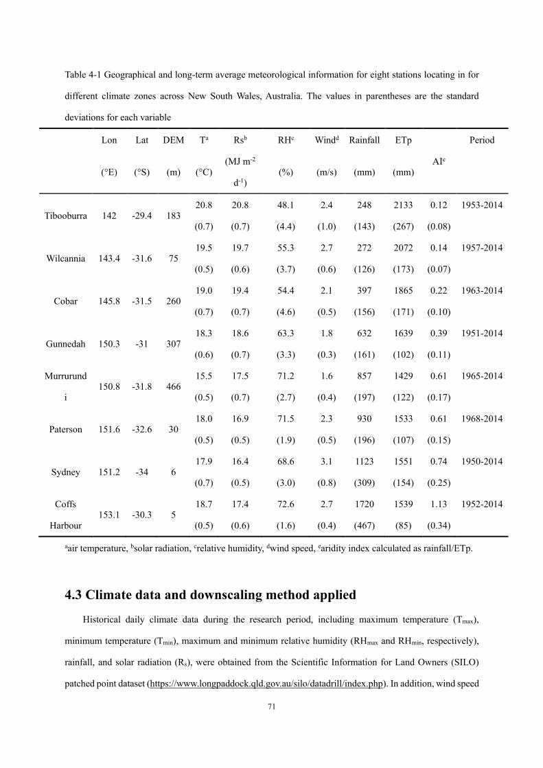
71

Table 4-1 Geographical and long-term average meteorological information for eight stations locating in for

different climate zones across New South Wales, Australia. The values in parentheses are the standard

deviations for each variable

Lon Lat DEM Ta Rsb RHc Windd Rainfall ETp

AIe

Period

(°E) (°S) (m) (°C)

(MJ m-2

d-1) (%) (m/s) (mm) (mm)

Tibooburra 142 -29.4 183 20.8

(0.7)

20.8

(0.7)

48.1

(4.4)

2.4

(1.0)

248

(143)

2133

(267)

0.12

(0.08)

1953-2014

Wilcannia 143.4 -31.6 75 19.5

(0.5)

19.7

(0.6)

55.3

(3.7)

2.7

(0.6)

272

(126)

2072

(173)

0.14

(0.07)

1957-2014

Cobar 145.8 -31.5 260 19.0

(0.7)

19.4

(0.7)

54.4

(4.6)

2.1

(0.5)

397

(156)

1865

(171)

0.22

(0.10)

1963-2014

Gunnedah 150.3 -31 307 18.3

(0.6)

18.6

(0.7)

63.3

(3.3)

1.8

(0.3)

632

(161)

1639

(102)

0.39

(0.11)

1951-2014

Murrurund

i 150.8 -31.8 466

15.5

(0.5)

17.5

(0.7)

71.2

(2.7)

1.6

(0.4)

857

(197)

1429

(122)

0.61

(0.17)

1965-2014

Paterson 151.6 -32.6 30 18.0

(0.5)

16.9

(0.5)

71.5

(1.9)

2.3

(0.5)

930

(196)

1533

(107)

0.61

(0.15)

1968-2014

Sydney 151.2 -34 6 17.9

(0.7)

16.4

(0.5)

68.6

(3.0)

3.1

(0.8)

1123

(309)

1551

(154)

0.74

(0.25)

1950-2014

Coffs

Harbour 153.1 -30.3 5

18.7

(0.5)

17.4

(0.6)

72.6

(1.6)

2.7

(0.4)

1720

(467)

1539

(85)

1.13

(0.34)

1952-2014

aair temperature, bsolar radiation, crelative humidity, dwind speed, earidity index calculated as rainfall/ETp.

4.3 Climate data and downscaling method applied

Historical daily climate data during the research period, including maximum temperature (Tmax),

minimum temperature (Tmin), maximum and minimum relative humidity (RHmax and RHmin, respectively),

rainfall, and solar radiation (Rs), were obtained from the Scientific Information for Land Owners (SILO)

patched point dataset (https://www.longpaddock.qld.gov.au/silo/datadrill/index.php). In addition, wind speed

72

data were obtained from the Bureau of Meteorology (BOM, http://www.bom.gov.au/). The percentage of

missing daily wind speed data was less than 5% for each station. To estimate the missing wind speed values,

we first used years with consecutive daily wind speed to calculate the long-term average wind speed for each

day of the year. Then we used the average wind speed for the i-th (i ranges from 1 to 365) day of the year as

the proxy wind speed for that day of the year with a missing value. To project ETp under future climate

scenarios, we downscaled 34 GCMs (Table 4-2) from the Coupled Model Intercomparison Project Phase 5

(CMIP5) dataset to extract daily Tmax, Tmin, rainfall, and Rs from 1900-2100 based on the statistical

downscaling method developed by Liu and Zuo (2012).

Statistical downscaling is an effective method to downscale the raw monthly climatic data from GCMs

at coarse spatial resolutions to a finer spatial and temporal scale. Firstly, the monthly climatic data from

GCMs were downscaled to specific sites using the inverse distance weighted interpolation method. Then bias

correction was applied to the monthly values of climatic factors for each site. Thirdly, we used a stochastic

weather generator to produce daily climatic factors for each site. The detailed information about this method

has been described by Liu and Zuo (2012). This study used the downscaled data to project future ETp with

the chosen empirical and machine learning-based ETp models under RCP4.5 and RCP8.5 climate scenarios.

For data downscaled from 34 GCMs, we defined the period from 1990 to 2014 as the baseline period.

The near future projected period was defined as 2026 to 2050 (2040s); the medium projected period was

from 2051 to 2075 (2065s); and the far future period was 2076-2100 (2090s).

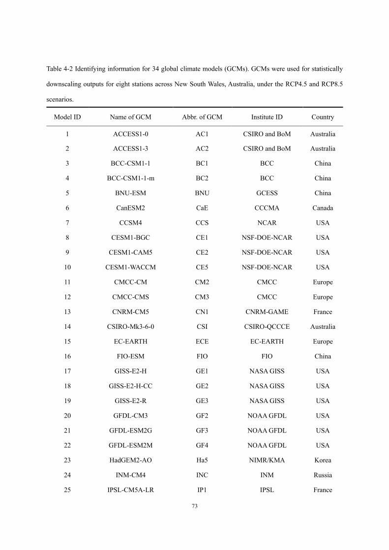
73

Table 4-2 Identifying information for 34 global climate models (GCMs). GCMs were used for statistically

downscaling outputs for eight stations across New South Wales, Australia, under the RCP4.5 and RCP8.5

scenarios.

Model ID Name of GCM Abbr. of GCM Institute ID Country

1 ACCESS1-0 AC1 CSIRO and BoM Australia

2 ACCESS1-3 AC2 CSIRO and BoM Australia

3 BCC-CSM1-1 BC1 BCC China

4 BCC-CSM1-1-m BC2 BCC China

5 BNU-ESM BNU GCESS China

6 CanESM2 CaE CCCMA Canada

7 CCSM4 CCS NCAR USA

8 CESM1-BGC CE1 NSF-DOE-NCAR USA

9 CESM1-CAM5 CE2 NSF-DOE-NCAR USA

10 CESM1-WACCM CE5 NSF-DOE-NCAR USA

11 CMCC-CM CM2 CMCC Europe

12 CMCC-CMS CM3 CMCC Europe

13 CNRM-CM5 CN1 CNRM-GAME France

14 CSIRO-Mk3-6-0 CSI CSIRO-QCCCE Australia

15 EC-EARTH ECE EC-EARTH Europe

16 FIO-ESM FIO FIO China

17 GISS-E2-H GE1 NASA GISS USA

18 GISS-E2-H-CC GE2 NASA GISS USA

19 GISS-E2-R GE3 NASA GISS USA

20 GFDL-CM3 GF2 NOAA GFDL USA

21 GFDL-ESM2G GF3 NOAA GFDL USA

22 GFDL-ESM2M GF4 NOAA GFDL USA

23 HadGEM2-AO Ha5 NIMR/KMA Korea

24 INM-CM4 INC INM Russia

25 IPSL-CM5A-LR IP1 IPSL France

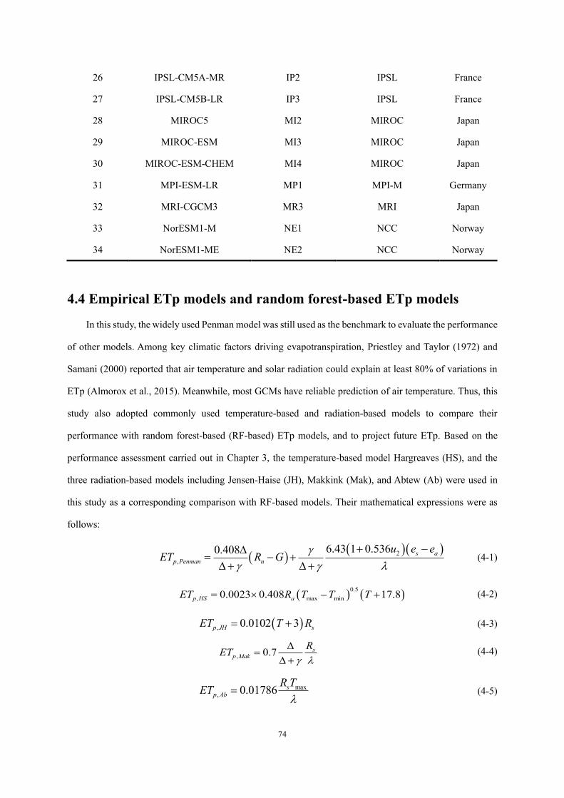
74

26 IPSL-CM5A-MR IP2 IPSL France

27 IPSL-CM5B-LR IP3 IPSL France

28 MIROC5 MI2 MIROC Japan

29 MIROC-ESM MI3 MIROC Japan

30 MIROC-ESM-CHEM MI4 MIROC Japan

31 MPI-ESM-LR MP1 MPI-M Germany

32 MRI-CGCM3 MR3 MRI Japan

33 NorESM1-M NE1 NCC Norway

34 NorESM1-ME NE2 NCC Norway

4.4 Empirical ETp models and random forest-based ETp models

In this study, the widely used Penman model was still used as the benchmark to evaluate the performance

of other models. Among key climatic factors driving evapotranspiration, Priestley and Taylor (1972) and

Samani (2000) reported that air temperature and solar radiation could explain at least 80% of variations in

ETp (Almorox et al., 2015). Meanwhile, most GCMs have reliable prediction of air temperature. Thus, this

study also adopted commonly used temperature-based and radiation-based models to compare their

performance with random forest-based (RF-based) ETp models, and to project future ETp. Based on the

performance assessment carried out in Chapter 3, the temperature-based model Hargreaves (HS), and the

three radiation-based models including Jensen-Haise (JH), Makkink (Mak), and Abtew (Ab) were used in

this study as a corresponding comparison with RF-based models. Their mathematical expressions were as

follows:

( )( )( )2

,

6.43 1 0.5360.408 s ap Penman n

u e eET R G

+ −= − +

+ + (4-1)

( ) ( )0.5

, max min0.0023 0.408 17.8p HS aET R T T T= − + (4-2)

( ), 0.0102 3p JH sET T R= + (4-3)

, 0.7 sp Mak

RET

=

+ (4-4)

max, 0.01786 s

p AbR TET

= (4-5)

75

where △ (kPa °C-1) is the slope of the saturation vapor pressure curve, determined by air temperature (T);

γ (kPa °C-1) is the psychrometric constant; Rn (MJ m-2 day-1) is net radiation determined according to Allen

et al. (1998); G (MJ m-2 day-1) is soil heat flux density, assumed to equal zero for periods of a day or longer;

u2 (m s-1) is wind speed at 2 m height; es (kPa) is saturation vapor pressure, determined by T; ea (kPa) is actual

vapor pressure, determined by T and relative humidity (RH); (es-ea) (kPa) is saturation vapor pressure deficit;

and 𝜆 is the latent heat of vaporization of water, which is calculated as a function of T, value of 2.45 MJ kg-

1 for T around 20°C; Tmax (°C) and Tmin (°C) are maximum temperature and minimum temperature,

respectively.

Random forest (RF) is one of the tree-based machine learning methods developed by Breiman (2001).

Compared with most well-established machine learning methods (e.g., artificial neural networks and SVM),

RF only needs two parameters: the number of decision trees (ntree) and the number of variables (mtry).

Moreover, RF has a strong predictive power to deal with non-linear and hierarchical relationships between

the predictors and the response. In fact, RF has been widely used for classification and regression tasks (Fan

et al., 2018; Heung et al., 2014; Wang et al., 2018b). Thus, we adopted RF as a representative machine

learning technique to estimate ETp in this study. Briefly, around 2/3 of the original data were randomly

chosen as the “bootstrapped” dataset to generate numerous decision trees (ntree) with a random subset of the

total variables (mtry) each step. Thus, a variety of decision trees were generated that formed the “Forest”. The

remaining original data (around 1/3), which were not chosen to build the “bootstrapped” dataset (known as

the “Out-of-Bag Dataset”) were used for validation. Based on the “Forest”, the projector used predicted data

and ran those data through all of the decision trees. The final prediction was the average of the results of all

trees. More information about RF can be found in Breiman (2001), and a schematic diagram of RF is shown

in Figure 4-2.

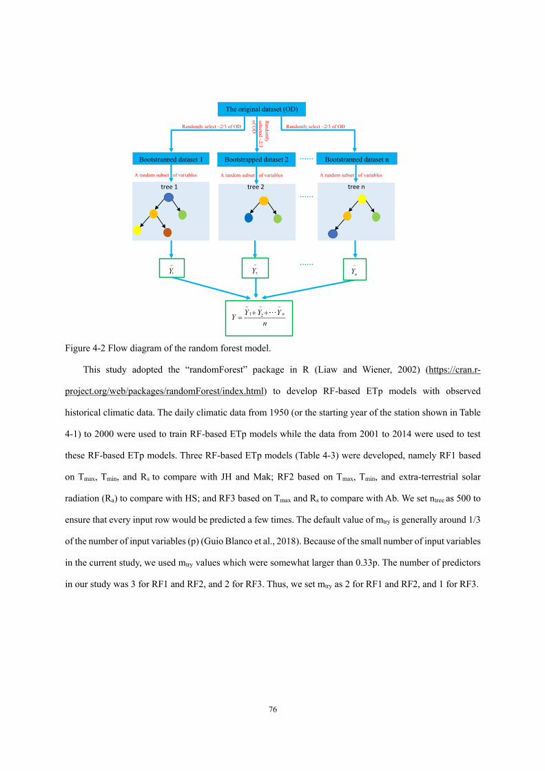
76

Figure 4-2 Flow diagram of the random forest model.

This study adopted the “randomForest” package in R (Liaw and Wiener, 2002) (https://cran.r-

project.org/web/packages/randomForest/index.html) to develop RF-based ETp models with observed

historical climatic data. The daily climatic data from 1950 (or the starting year of the station shown in Table

4-1) to 2000 were used to train RF-based ETp models while the data from 2001 to 2014 were used to test

these RF-based ETp models. Three RF-based ETp models (Table 4-3) were developed, namely RF1 based

on Tmax, Tmin, and Rs to compare with JH and Mak; RF2 based on Tmax, Tmin, and extra-terrestrial solar

radiation (Ra) to compare with HS; and RF3 based on Tmax and Rs to compare with Ab. We set ntree as 500 to

ensure that every input row would be predicted a few times. The default value of mtry is generally around 1/3

of the number of input variables (p) (Guio Blanco et al., 2018). Because of the small number of input variables

in the current study, we used mtry values which were somewhat larger than 0.33p. The number of predictors

in our study was 3 for RF1 and RF2, and 2 for RF3. Thus, we set mtry as 2 for RF1 and RF2, and 1 for RF3.

The original dataset (OD)

Bootstrapped dataset 1 Bootstrapped dataset 2 Bootstrapped dataset n ……

Randomly select ~2/3 of OD Randomly select ~2/3 of OD

Random

ly selected ~2/3 of O

D

A random subset of variables A random subset of variables A random subset of variables

tree 1 tree 2 tree n ……

1Y−

……

1 2 nY Y YYn

− − −

+ +=

2Y−

nY−

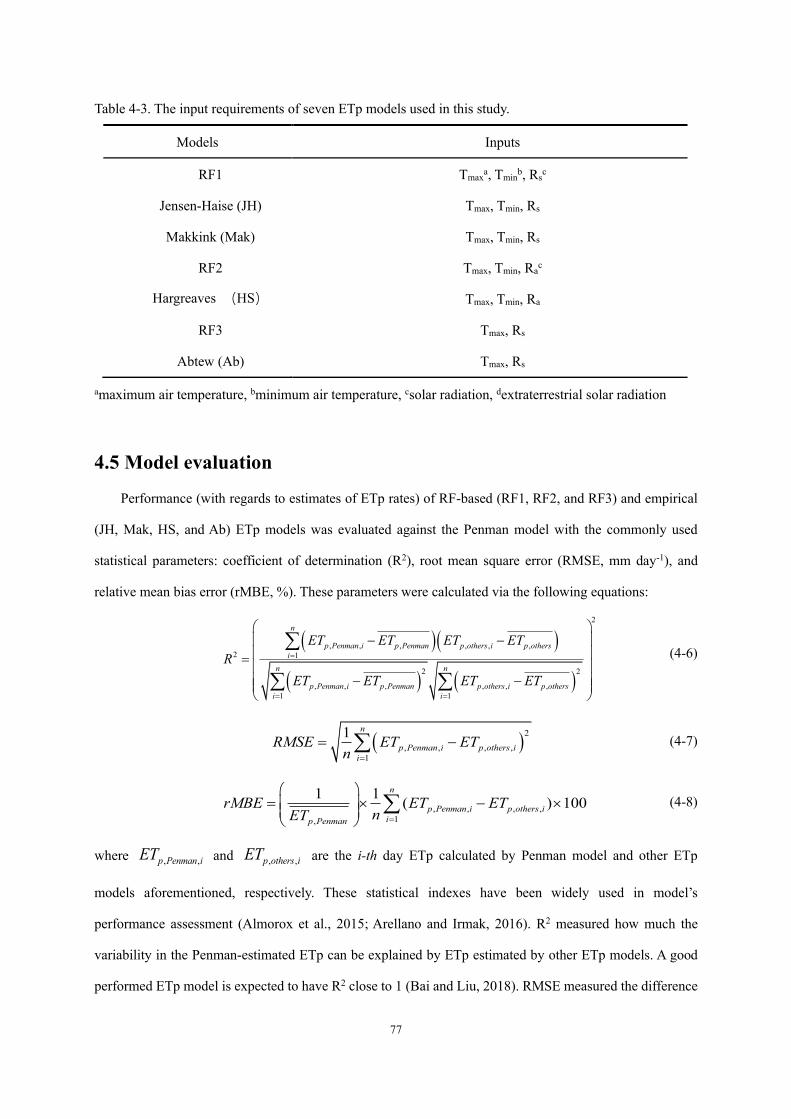
77

Table 4-3. The input requirements of seven ETp models used in this study.

amaximum air temperature, bminimum air temperature, csolar radiation, dextraterrestrial solar radiation

4.5 Model evaluation

Performance (with regards to estimates of ETp rates) of RF-based (RF1, RF2, and RF3) and empirical

(JH, Mak, HS, and Ab) ETp models was evaluated against the Penman model with the commonly used

statistical parameters: coefficient of determination (R2), root mean square error (RMSE, mm day-1), and

relative mean bias error (rMBE, %). These parameters were calculated via the following equations:

( )( )

( ) ( )

2

, , , , , ,2 1

2 2

, , , , , ,1 1

n

p Penman i p Penman p others i p othersi

n n

p Penman i p Penman p others i p othersi i

ET ET ET ETR

ET ET ET ET

=

= =

− − = − −

(4-6)

( )2

, , , ,1

1 n

p Penman i p others ii

RMSE ET ETn =

= − (4-7)

, , , ,1,

1 1 ( ) 100n

p Penman i p others iip Penman

rMBE ET ETnET =

= −

(4-8)

where , ,p Penman iET and , ,p others iET are the i-th day ETp calculated by Penman model and other ETp

models aforementioned, respectively. These statistical indexes have been widely used in model’s

performance assessment (Almorox et al., 2015; Arellano and Irmak, 2016). R2 measured how much the

variability in the Penman-estimated ETp can be explained by ETp estimated by other ETp models. A good

performed ETp model is expected to have R2 close to 1 (Bai and Liu, 2018). RMSE measured the difference

Models Inputs

RF1 Tmaxa, Tminb, Rsc

Jensen-Haise (JH) Tmax, Tmin, Rs

Makkink (Mak) Tmax, Tmin, Rs

RF2 Tmax, Tmin, Rac

Hargreaves （HS） Tmax, Tmin, Ra

RF3 Tmax, Rs

Abtew (Ab) Tmax, Rs

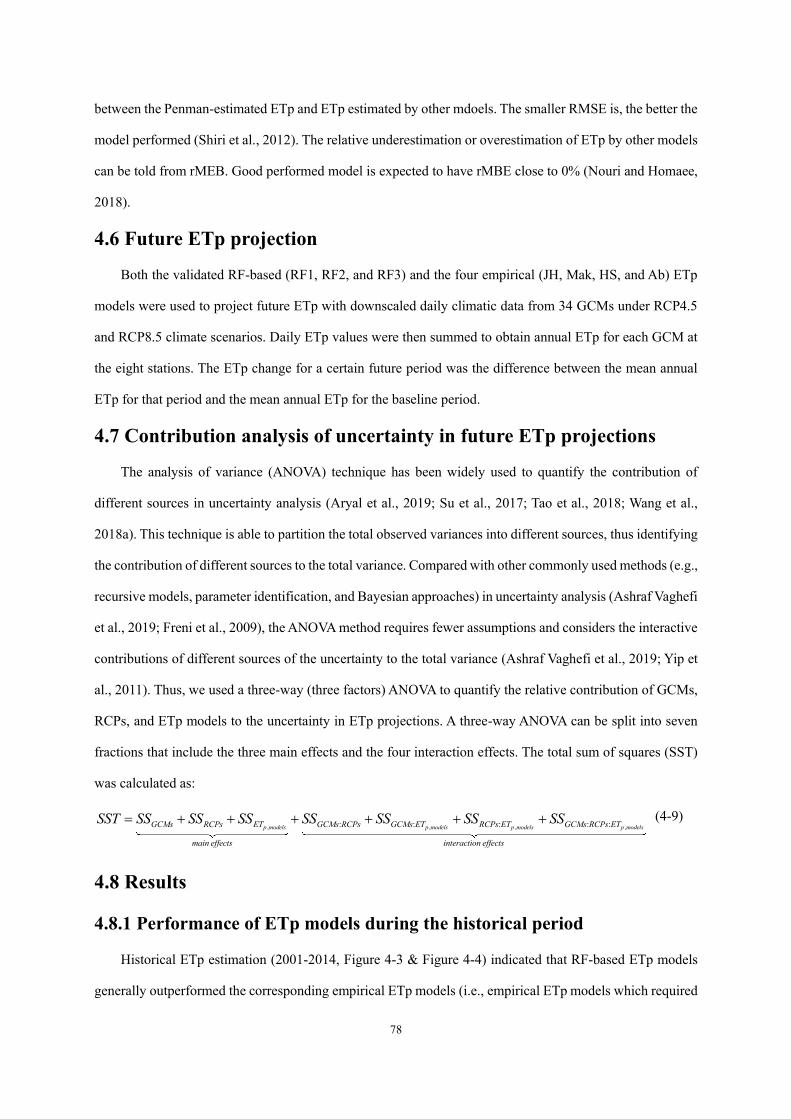
78

between the Penman-estimated ETp and ETp estimated by other mdoels. The smaller RMSE is, the better the

model performed (Shiri et al., 2012). The relative underestimation or overestimation of ETp by other models

can be told from rMEB. Good performed model is expected to have rMBE close to 0% (Nouri and Homaee,

2018).

4.6 Future ETp projection

Both the validated RF-based (RF1, RF2, and RF3) and the four empirical (JH, Mak, HS, and Ab) ETp

models were used to project future ETp with downscaled daily climatic data from 34 GCMs under RCP4.5

and RCP8.5 climate scenarios. Daily ETp values were then summed to obtain annual ETp for each GCM at

the eight stations. The ETp change for a certain future period was the difference between the mean annual

ETp for that period and the mean annual ETp for the baseline period.

4.7 Contribution analysis of uncertainty in future ETp projections

The analysis of variance (ANOVA) technique has been widely used to quantify the contribution of

different sources in uncertainty analysis (Aryal et al., 2019; Su et al., 2017; Tao et al., 2018; Wang et al.,

2018a). This technique is able to partition the total observed variances into different sources, thus identifying

the contribution of different sources to the total variance. Compared with other commonly used methods (e.g.,

recursive models, parameter identification, and Bayesian approaches) in uncertainty analysis (Ashraf Vaghefi

et al., 2019; Freni et al., 2009), the ANOVA method requires fewer assumptions and considers the interactive

contributions of different sources of the uncertainty to the total variance (Ashraf Vaghefi et al., 2019; Yip et

al., 2011). Thus, we used a three-way (three factors) ANOVA to quantify the relative contribution of GCMs,

RCPs, and ETp models to the uncertainty in ETp projections. A three-way ANOVA can be split into seven

fractions that include the three main effects and the four interaction effects. The total sum of squares (SST)

was calculated as:

, , , ,: : : : :p models p models p models p modelsGCMs RCPs ET GCMs RCPs GCMs ET RCPs ET GCMs RCPs ET

main effects interaction effects

SST SS SS SS SS SS SS SS= + + + + + + (4-9)

4.8 Results

4.8.1 Performance of ETp models during the historical period

Historical ETp estimation (2001-2014, Figure 4-3 & Figure 4-4) indicated that RF-based ETp models

generally outperformed the corresponding empirical ETp models (i.e., empirical ETp models which required

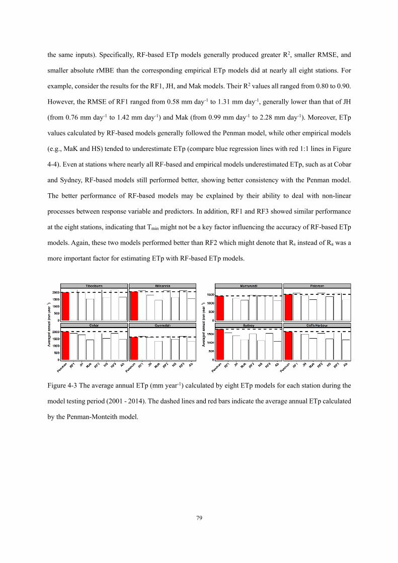
79

the same inputs). Specifically, RF-based ETp models generally produced greater R2, smaller RMSE, and

smaller absolute rMBE than the corresponding empirical ETp models did at nearly all eight stations. For

example, consider the results for the RF1, JH, and Mak models. Their R2 values all ranged from 0.80 to 0.90.

However, the RMSE of RF1 ranged from 0.58 mm day-1 to 1.31 mm day-1, generally lower than that of JH

(from 0.76 mm day-1 to 1.42 mm day-1) and Mak (from 0.99 mm day-1 to 2.28 mm day-1). Moreover, ETp

values calculated by RF-based models generally followed the Penman model, while other empirical models

(e.g., MaK and HS) tended to underestimate ETp (compare blue regression lines with red 1:1 lines in Figure

4-4). Even at stations where nearly all RF-based and empirical models underestimated ETp, such as at Cobar

and Sydney, RF-based models still performed better, showing better consistency with the Penman model.

The better performance of RF-based models may be explained by their ability to deal with non-linear

processes between response variable and predictors. In addition, RF1 and RF3 showed similar performance

at the eight stations, indicating that Tmin might not be a key factor influencing the accuracy of RF-based ETp

models. Again, these two models performed better than RF2 which might denote that Rs instead of Ra was a

more important factor for estimating ETp with RF-based ETp models.

Figure 4-3 The average annual ETp (mm year-1) calculated by eight ETp models for each station during the

model testing period (2001 - 2014). The dashed lines and red bars indicate the average annual ETp calculated

by the Penman-Monteith model.

80

Figure 4-4. Scatter plots of the Penman-calculated daily ETp (mm day-1) vs ETp calculated by RF-based and

empirical ETp models during the model testing stage (2001 - 2014) for each of eight stations in New South

Wales, Australia. The units for RMSE and rMBE are mm day-1 and %, respectively. Blue lines are linear

regression lines and red lines are 1:1 lines.

4.8.2 The change of climatic factors under future climate scenarios

Consistent increases were observed in Tmax (Figure 4-5a) and Tmin (Figure 4-5b) irrespective of RCP

scenarios and stations. Specifically, the increases of mean Tmax ranged from 0.61 °C by the 2040s to 2.33 °C

by the 2090s under RCP4.5 while the range for mean Tmin was 0.88 °C (2040s) to 2.02 °C (2090s). Under

RMSE = 0.58 rMBE = 0.50 R2 = 0.91

RMSE = 0.83 rMBE = 4.57 R2 = 0.85

RMSE = 0.83 rMBE = 4.57 R2 = 0.85

RMSE = 0.76 rMBE = -5.63 R2 = 0.85

RMSE = 0.76 rMBE = -5.63 R2 = 0.85

RMSE = 0.83 rMBE = -5.57 R2 = 0.87

RMSE = 1.41 rMBE = -21.20 R2 = 0.81

RMSE = 0.89 rMBE = -9.19 R2 = 0.84

RMSE = 0.99 rMBE = -17.22 R2 = 0.89

RMSE = 1.24 rMBE = -20.68 R2 = 0.85

RMSE = 2.01 rMBE = -34.44 R2 = 0.79

RMSE = 1.37 rMBE = -24.09 R2 = 0.82

RMSE = 0.80 rMBE = 2.36 R2 = 0.84

RMSE = 1.12 rMBE = 5.34 R2 = 0.72

RMSE = 1.46 rMBE = -16.10 R2 = 0.68

RMSE = 1.03 rMBE = -6.07 R2 = 0.72

RMSE = 0.79 rMBE = 0.67 R2 = 0.84

RMSE = 1.06 rMBE = -8.77 R2 = 0.77

RMSE = 2.21 rMBE = -37.61 R2 = 0.71

RMSE = 1.57 rMBE = -26.09 R2 = 0.72

RMSE = 0.61 rMBE = 0.78 R2 = 0.90

RMSE = 0.96 rMBE = -18.87 R2 = 0.90

RMSE = 0.84 rMBE = 4.19 R2 = 0.85

RMSE = 1.18 rMBE = -21.14 R2 = 0.86

RMSE = 1.14 rMBE = -13.92 R2 = 0.83

RMSE = 2.19 rMBE = -40.11 R2 = 0.82

RMSE = 0.78 rMBE = -5.48 R2 = 0.84

RMSE = 1.54 rMBE = -29.47 R2 = 0.84

RMSE = 1.23 rMBE = 0.24 R2 = 0.83

RMSE = 1.23 rMBE = 9.27 R2 = 0.83

RMSE = 1.81 rMBE = -23.13 R2 = 0.81

RMSE = 1.39 rMBE = 9.73 R2 = 0.78

RMSE = 1.62 rMBE = -17.93 R2 = 0.76

RMSE = 1.20 rMBE = 9.17 R2 = 0.83

RMSE = 1.50 rMBE = -17.43 R2 = 0.80

RMSE = 1.31 rMBE = 4.47 R2 = 0.81

RMSE = 1.42 rMBE = -11.64 R2 = 0.82

RMSE = 2.28 rMBE = -29.56 R2 = 0.80

RMSE = 1.41 rMBE = 3.73 R2 = 0.78

RMSE = 1.85 rMBE = -19.84 R2 = 0.75

RMSE = 1.30 rMBE = 4.05 R2 = 0.81

RMSE = 1.90 rMBE = -23.99 R2 = 0.79

RMSE = 0.84 rMBE = -6.55 R2 = 0.92

RMSE = 1.07 rMBE = -11.91 R2 = 0.91

RMSE = 2.07 rMBE = -29.23 R2 = 0.87

RMSE = 0.99 rMBE = -7.00 R2 = 0.89

RMSE = 1.69 rMBE = -24.30 R2 = 0.89

RMSE = 0.86 rMBE = -6.31 R2 = 0.92

RMSE = 1.75 rMBE = -26.90 R2 = 0.90

RMSE = 0.91 rMBE = 3.18 R2 = 0.84

RMSE = 0.97 rMBE = -1.38 R2 = 0.85

RMSE = 1.32 rMBE = -18.44 R2 = 0.82

RMSE = 1.04 rMBE = 3.78 R2 = 0.79

RMSE = 1.10 rMBE = -9.78 R2 = 0.80

RMSE = 0.91 rMBE = 2.97 R2 = 0.84

RMSE = 1.22 rMBE = -18.13 R2 = 0.83

81

RCP8.5, larger increases were found in both Tmax and Tmin than under RCP4.5 for a certain future period. For

instance, the range of increases of mean Tmax and mean Tmin under RCP8.5 were 0.79 °C (2040s) to 4.58 °C

(2090s) and 1.10 °C (2040s) to 4.39 °C (2090s), respectively. Moreover, as time increased into the future

period, the increase in Tmax and Tmin became larger. Similar increasing trends were also found in Rs,

independent of stations. Mean Rs (Figure 4-6a) was projected to increase by 0.08-0.32 MJ m-2 day-1 under

RCP4.5 and 0.01-0.29 MJ m-2 day-1 under RCP8.5.

82

Figure 4-5. Projected changes in Tmax (℃), Tmin (℃), and Tmax-Tmin (℃) in the near future (2026 – 2050,

2040s), the medium future (2051 – 2075, 2065s), and the far future (2076 – 2100, 2090s) at eight stations in

New South Wales, Australia, under RCP4.5 and RCP8.5 scenarios based on 34 GCMs compared with

baseline values (1990 - 2014). Lower and upper box boundaries indicate the 25th and 75th percentiles,

respectively. The black lines and dots inside the box mark the median and mean, respectively. The lower and

upper whiskers indicate the 10th and 90th percentiles, respectively.

In contrast to the uniform increase in Tmax and Tmin was the obvious difference found among stations in

the direction and magnitude of change of ΔT over time (Figure 4-5c). For instance, mean ΔT at Murrurundi

increased by 0.14-0.31 °C under RCP4.5 and by 0.12-0.18 °C under RCP8.5 whereas it decreased by 0.36-

(a)

(b)

(c)

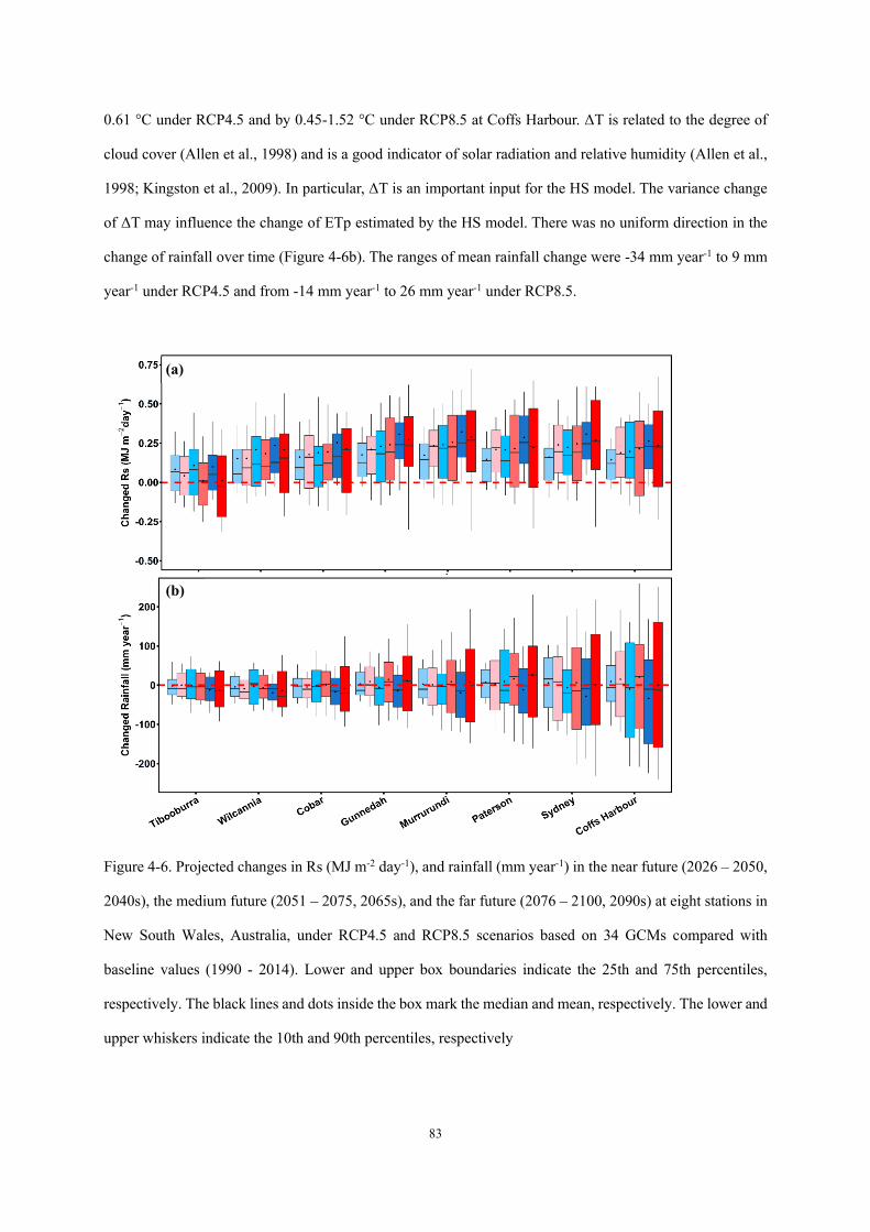
83

0.61 °C under RCP4.5 and by 0.45-1.52 °C under RCP8.5 at Coffs Harbour. ΔT is related to the degree of

cloud cover (Allen et al., 1998) and is a good indicator of solar radiation and relative humidity (Allen et al.,

1998; Kingston et al., 2009). In particular, ΔT is an important input for the HS model. The variance change

of ΔT may influence the change of ETp estimated by the HS model. There was no uniform direction in the

change of rainfall over time (Figure 4-6b). The ranges of mean rainfall change were -34 mm year-1 to 9 mm

year-1 under RCP4.5 and from -14 mm year-1 to 26 mm year-1 under RCP8.5.

Figure 4-6. Projected changes in Rs (MJ m-2 day-1), and rainfall (mm year-1) in the near future (2026 – 2050,

2040s), the medium future (2051 – 2075, 2065s), and the far future (2076 – 2100, 2090s) at eight stations in

New South Wales, Australia, under RCP4.5 and RCP8.5 scenarios based on 34 GCMs compared with

baseline values (1990 - 2014). Lower and upper box boundaries indicate the 25th and 75th percentiles,

respectively. The black lines and dots inside the box mark the median and mean, respectively. The lower and

upper whiskers indicate the 10th and 90th percentiles, respectively

(a))

(b)

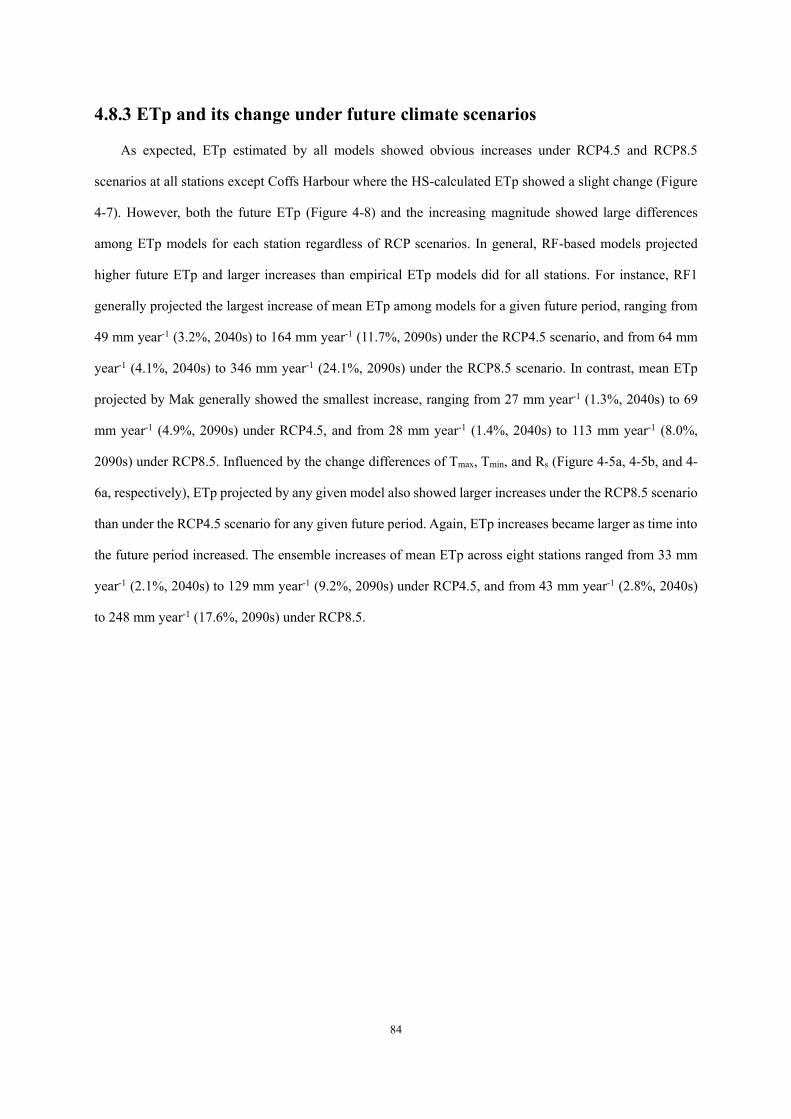
84

4.8.3 ETp and its change under future climate scenarios

As expected, ETp estimated by all models showed obvious increases under RCP4.5 and RCP8.5

scenarios at all stations except Coffs Harbour where the HS-calculated ETp showed a slight change (Figure

4-7). However, both the future ETp (Figure 4-8) and the increasing magnitude showed large differences

among ETp models for each station regardless of RCP scenarios. In general, RF-based models projected

higher future ETp and larger increases than empirical ETp models did for all stations. For instance, RF1

generally projected the largest increase of mean ETp among models for a given future period, ranging from

49 mm year-1 (3.2%, 2040s) to 164 mm year-1 (11.7%, 2090s) under the RCP4.5 scenario, and from 64 mm

year-1 (4.1%, 2040s) to 346 mm year-1 (24.1%, 2090s) under the RCP8.5 scenario. In contrast, mean ETp

projected by Mak generally showed the smallest increase, ranging from 27 mm year-1 (1.3%, 2040s) to 69

mm year-1 (4.9%, 2090s) under RCP4.5, and from 28 mm year-1 (1.4%, 2040s) to 113 mm year-1 (8.0%,

2090s) under RCP8.5. Influenced by the change differences of Tmax, Tmin, and Rs (Figure 4-5a, 4-5b, and 4-

6a, respectively), ETp projected by any given model also showed larger increases under the RCP8.5 scenario

than under the RCP4.5 scenario for any given future period. Again, ETp increases became larger as time into

the future period increased. The ensemble increases of mean ETp across eight stations ranged from 33 mm

year-1 (2.1%, 2040s) to 129 mm year-1 (9.2%, 2090s) under RCP4.5, and from 43 mm year-1 (2.8%, 2040s)

to 248 mm year-1 (17.6%, 2090s) under RCP8.5.

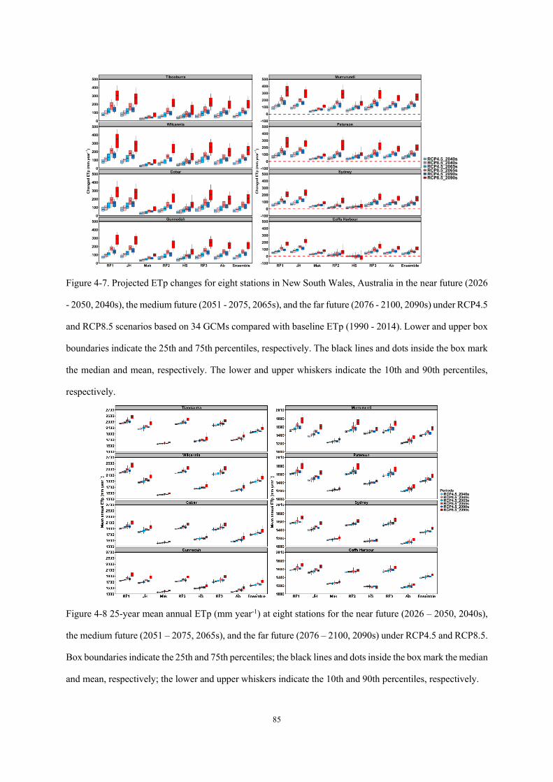
85

Figure 4-7. Projected ETp changes for eight stations in New South Wales, Australia in the near future (2026

- 2050, 2040s), the medium future (2051 - 2075, 2065s), and the far future (2076 - 2100, 2090s) under RCP4.5

and RCP8.5 scenarios based on 34 GCMs compared with baseline ETp (1990 - 2014). Lower and upper box

boundaries indicate the 25th and 75th percentiles, respectively. The black lines and dots inside the box mark

the median and mean, respectively. The lower and upper whiskers indicate the 10th and 90th percentiles,

respectively.

Figure 4-8 25-year mean annual ETp (mm year-1) at eight stations for the near future (2026 – 2050, 2040s),

the medium future (2051 – 2075, 2065s), and the far future (2076 – 2100, 2090s) under RCP4.5 and RCP8.5.

Box boundaries indicate the 25th and 75th percentiles; the black lines and dots inside the box mark the median

and mean, respectively; the lower and upper whiskers indicate the 10th and 90th percentiles, respectively.

86

4.8.4 Contribution of climatic factors to ETp change

The influence of a certain climatic factor on ETp change projection may be varied among ETp models.

Guo et al. (2017) analyzed the sensitivity Penman-Monteith and Priestley-Taylor to different climatic factors

with the use of global sensitivity analysis across different climatic zones in Australia. They found that

temperature is the most important factor resulting in the changes of ETp in Australia. Models used in this

thesis to project ETp under future climate scenarios are either temperature-based or radiation-based.

Meanwhile, downscaled climatic data used in this study to project future ETp only included maximum and

minimum temperatures, solar radiation. Thus, we only focused on the contribution of temperature and

radiation, which can be more reliably projected by GCMs to changes of ETp under future climate scenarios.

In order to determine the relationships between the change of ETp and changes of meteorological factors,

multiple linear regression was performed for each station using changes of Tmax, Tmin, Rs, and rainfall as

independent variables and changes of ETp as the dependent variable. Our analysis showed that changes in

Tmax, Tmin, Rs, and rainfall generally accounted for more than 92.0% of the ETp change, and the change of

rainfall had only a slight influence in ETp for most stations (Figure 4-9). We also found that relationships

between the change of Tmax, Tmin, and Rs and the change of ETp could be grouped based on the input

requirements of ETp models. In general, compared with Tmax and Tmin, a unit increase of Rs led to a larger

increase of ETp projected by RF1, JH, and Mak. In contrarst, the largest ETp increases (ranging from 64.0

mm year-1 to 116.7 mm year-1) projected by RF2 and HS were caused by a unit increase of Tmax, while changes

in Tmin and Rs were negatively related to ETp changes. Lastly, for RF3 and Ab, one unit increase in Rs and

Tmax could contribute roughly equally to the change in ETp.

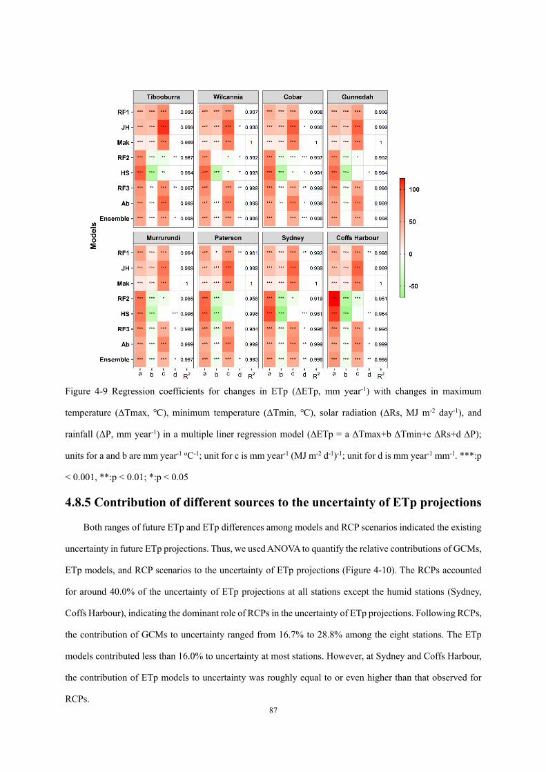
87

Figure 4-9 Regression coefficients for changes in ETp (ΔETp, mm year-1) with changes in maximum

temperature (ΔTmax, ℃), minimum temperature (ΔTmin, ℃), solar radiation (ΔRs, MJ m-2 day-1), and

rainfall (ΔP, mm year-1) in a multiple liner regression model (ΔETp = a ΔTmax+b ΔTmin+c ΔRs+d ΔP);

units for a and b are mm year-1 oC-1; unit for c is mm year-1 (MJ m-2 d-1)-1; unit for d is mm year-1 mm-1. ***:p

< 0.001, **:p < 0.01; *:p < 0.05

4.8.5 Contribution of different sources to the uncertainty of ETp projections

Both ranges of future ETp and ETp differences among models and RCP scenarios indicated the existing

uncertainty in future ETp projections. Thus, we used ANOVA to quantify the relative contributions of GCMs,

ETp models, and RCP scenarios to the uncertainty of ETp projections (Figure 4-10). The RCPs accounted

for around 40.0% of the uncertainty of ETp projections at all stations except the humid stations (Sydney,

Coffs Harbour), indicating the dominant role of RCPs in the uncertainty of ETp projections. Following RCPs,

the contribution of GCMs to uncertainty ranged from 16.7% to 28.8% among the eight stations. The ETp

models contributed less than 16.0% to uncertainty at most stations. However, at Sydney and Coffs Harbour,

the contribution of ETp models to uncertainty was roughly equal to or even higher than that observed for

RCPs.

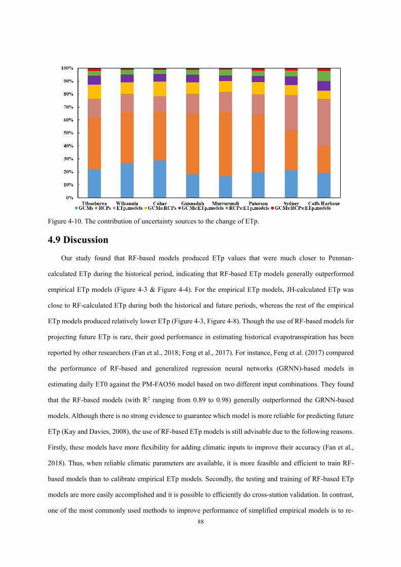
88

Figure 4-10. The contribution of uncertainty sources to the change of ETp.

4.9 Discussion

Our study found that RF-based models produced ETp values that were much closer to Penman-

calculated ETp during the historical period, indicating that RF-based ETp models generally outperformed

empirical ETp models (Figure 4-3 & Figure 4-4). For the empirical ETp models, JH-calculated ETp was

close to RF-calculated ETp during both the historical and future periods, whereas the rest of the empirical

ETp models produced relatively lower ETp (Figure 4-3, Figure 4-8). Though the use of RF-based models for

projecting future ETp is rare, their good performance in estimating historical evapotranspiration has been

reported by other researchers (Fan et al., 2018; Feng et al., 2017). For instance, Feng et al. (2017) compared

the performance of RF-based and generalized regression neural networks (GRNN)-based models in

estimating daily ET0 against the PM-FAO56 model based on two different input combinations. They found

that the RF-based models (with R2 ranging from 0.89 to 0.98) generally outperformed the GRNN-based

models. Although there is no strong evidence to guarantee which model is more reliable for predicting future

ETp (Kay and Davies, 2008), the use of RF-based ETp models is still advisable due to the following reasons.

Firstly, these models have more flexibility for adding climatic inputs to improve their accuracy (Fan et al.,

2018). Thus, when reliable climatic parameters are available, it is more feasible and efficient to train RF-

based models than to calibrate empirical ETp models. Secondly, the testing and training of RF-based ETp

models are more easily accomplished and it is possible to efficiently do cross-station validation. In contrast,

one of the most commonly used methods to improve performance of simplified empirical models is to re-

89

calibrate the empirical coefficients based on a linear relationship against observed ET or Penman-Monteith-

type models (Droogers and Allen, 2002; Tabari and Talaee, 2011). However, these coefficients are generally

location-specific and may result in less accurate performance in another region. Even if empirical coefficients

are calibrated for a certain station, the updated coefficients may vary with time due to climatic changes and

variations (Nouri and Homaee, 2018).

ETp projected by all models showed an overall increase under future climate scenarios and the increase

was the largest at the end of the 21st century under the RCP8.5 scenario (Figure 4-7). The increases in Tmax,

Tmin, and Rs all contributed to the upward trend of ETp (Pan et al., 2015; Scheff and Frierson, 2014), as shown

in Figure 4-9. Although ETp increases under future climate scenarios have been widely reported (Dong et al.,

2019; Gharbia et al., 2018; Pan et al., 2015; Scheff and Frierson, 2014; Tao et al., 2015; Wang et al., 2017b;

Wang et al., 2015), large variances and uncertainties were observed in the magnitudes of the increases. At the

global scale, Scheff and Frierson (2014) adopted the PM-FAO56 model with climatic data from 13 GCMs to

project the future ETp. They found ETp generally increased 10.0% to 45.0% by the end of the 21st century.

Also at the global scale, Pan et al. (2015) adopted the Dynamic Land Ecosystem Model to project future

global terrestrial evapotranspiration under the A2 and B1 emission scenarios. They found that compared with

the 2000s, terrestrial evapotranspiration by the 2090s would increase 14.0% under the A2 scenario and 4.5%

under the B1 scenario. In the Shannon River catchment, Ireland, Gharbia et al. (2018) adopted the Hamon

model with climatic data from multi-GCMs to project future ETp and found that ETp could increase up to

13.5% by the 2080s compared with ETp in 1961-2014. In Australia, Johnson and Sharma (2010) used outputs

from five GCMs to drive the PenPan model and projected open body water evaporation in the future. They

claimed that the average increase in open body water evaporation in 2070 would be approximately 7% under

the A2 scenario and 5% under the B1 scenario. In our study, the RF-based ETp models generally produced a

roughly comparable increase in ETp to that of the above-mentioned studies, ranging from 2.1% to 11.7%

under RCP4.5 and from 4.8% to 24.1% under RCP8.5 by the end of 21st century. As CSIRO and BOM (2015)

indicated, there was high confidence in the increase of ETp during this time period, but only medium

confidence was found for the magnitude of the increase.

The large uncertainty in future ETp projections may be due to differences in GCMs (Teng et al., 2012),

ETp models (Kingston et al., 2009), and RCPs (Wilby and Harris, 2006). Our study found that the dominant

reason leading to uncertainty in ETp projection was attributable to the differences in the RCP scenarios,

accounting for around 40% of the uncertainty (Figure 4-10). This result is likely due to the fact that predicted

90

changes of the major inputs (e.g., Tmax, Tmin, and Rs) for ETp models were clearly different under the different

RCPs (Figure 4-5 & Figure 4-6). It is well known that the GCMs we used in this study project raw monthly

climatic data such as air temperature and solar radiation that include uncertainties and biases that are

attributable to differences between GCMs and climate variables. However, we applied an improved statistical

downscaling method (Liu and Zuo, 2012) that effectively corrected biases in the GCM-projected climate

variables and matched observed climate while preserving the inter-annual and intra-seasonal variabilities of

GCM projections (Liu et al., 2017). This approach effectively minimized the additional uncertainty from the

downscaling method while the projected climate change signals were maintained for our analysis of GCM

uncertainties. In addition, we also found that the predictions of both climatic factors (Figure 4-5 & Figure 4-

6) and ETp (Figure 4-7 & Figure4-8) showed wider ranges under RCP8.5 than under RCP4.5, especially for

the 2090s. This might indicate that GCMs behaved more differently from each other under RCP8.5 in the

future (Shen et al., 2018), which might also contribute to the dominant role of RCPs in uncertainty of ETp

projection. Following RCPs, GCM-related and ETp model-related uncertainty contributed roughly equally

to ETp uncertainty, ranging from 10% to 30% (Figure 4-10). Similar to our results, Kingston et al. (2009)

projected global ETp with six alternative ETp models driven by data from five GCMs. They found that ETp

model-related uncertainty was of a similar magnitude or, in some cases, greater than GCM-related uncertainty.

Since ETp is an important input to hydrological models, the uncertainty in ETp projection may also influence

hydrological projections (Thompson et al., 2014), thus reducing the confidence in predictions of water

availability in the future. To deal with the uncertainty in future ETp projections, we recommend using

multiple GCMs to drive various ETp models under different RCP scenarios, so that a relatively reliable

projection is produced.

Quantifying the future increase in ETp can provide insights into future water availability and agricultural

production in NSW. For instance, increased ETp indicates that atmospheric evaporative demand will be

higher under future climate scenarios. However, both our study (Figure 3e) and other studies (Chiew et al.,

2009; Vaze and Teng, 2011) suggested that annual rainfall in NSW will not show significant increases in the

future. With the combined influence of increasing ETp and normal or even decreased rainfall, there is a high

possibility that runoff in NSW would decrease and this region would be drier (Teng et al., 2012). As Nicholls

(2004) put it, rising temperatures and increasing ETp, even without decreasing rainfall, would increase the

severity of droughts in Australia. Similarly, Feng et al. (2018a) projected changes of drought across the wheat

belt of NSW with climatic data from 28 GCMs under RCP8.5. They found that decreasing rainfall combined

91

with increasing temperature may lead to an expansion (from west to east) of the winter-spring drought-prone

areas. Furthermore, we found that the increase in ETp at the traditionally arid stations (e.g. Tibooburra and

Wilcannia, Figure 4-7) was larger than at the humid stations (e.g., Sydney & Coffs Harbour, Figure 4-7),

which might indicate that the traditionally dry areas might become drier at a faster rate than the humid areas.

One limitation of this study is that we did not consider the influence of increasing atmospheric CO2 on

stomatal conductance. A higher CO2 concentration will result in greater surface resistance (rs). This may

offset the magnitude of the ETp increases caused by the warming climate. In a recent study, Yang et al. (2019)

developed an equation to describe the relationship between rs and atmospheric CO2 concentration. Based on

the equation, they revised the PM-FAO56 model to consider the influence of increasing atmospheric CO2.

Their research offered a new perspective to assess the comprehensive impact of climate change on ETp and

should be considered in future studies.

4.10 Conclusions

This study developed RF-based ETp models and assessed their performance against four empirical ETp

models (JH, Mak, HS, and Ab), with the Penman-calculated ETp as a benchmark. The random forest-based

models and the four empirical ETp models were used to project ETp at eight stations across NSW using

climatic data from 34 GCMs under the RCP4.5 and RCP8.5 scenarios. Study results indicated that random

forest-based models generally outperformed the empirical ETp models in estimating historical daily Penman

ETp. Contrary to empirical ETp models, which was generally developed for a certain climate, random forest

models is easy to be trained at any kind of climate. Thus, the use of random forest method in ETp or drought

projection is promising not only in arid regions like Australia but also any other regions in the world. All of

these models projected that ETp would increase over time. However, the increased ETp estimates produced

by the random forest-based models better matched results obtained in other studies. The ensemble increases

of mean ETp across eight stations ranged from 33 mm year-1 (2.1%, 2040s) to 129 mm year-1 (9.2%, 2090s)

under RCP4.5, and from 43 mm year-1 (2.8%, 2040s) to 248 mm year-1 (17.6%, 2090s) under RCP8.5.

Furthermore, differences in RCPs accounted for around 40% of the uncertainty in future ETp projections due

to the great disparity in the expected temperature increases among the different emission scenarios. The large

uncertainty in the projected increases of ETp highlights the necessity of adopting multiple model ensemble

to project future ETp under different RCPs so that more reliable projections can be produced.

92

4.11 Reference Allen, R.G., Pereira, L.S., Raes, D., Smith, M., 1998. Crop evapotranspiration - Guidelines for computing Crop

Water Requirements. FAO Irrigation & Drainage Paper 56, Rome, Italy.

Almorox, J., Quej, V.H., Martí, P., 2015. Global performance ranking of temperature-based approaches for

evapotranspiration estimation considering Köppen climate classes. Journal of Hydrology, 528: 514-

522. DOI:https://doi.org/10.1016/j.jhydrol.2015.06.057

Arellano, M.G., Irmak, S., 2016. Reference (Potential) Evapotranspiration. I: Comparison of Temperature,

Radiation, and Combination-Based Energy Balance Equations in Humid, Subhumid, Arid, Semiarid,

and Mediterranean-Type Climates. Journal of Irrigation and Drainage Engineering, 142(4):

04015065. DOI:doi:10.1061/(ASCE)IR.1943-4774.0000978

Arnell, N.W., Gosling, S.N., 2013. The impacts of climate change on river flow regimes at the global scale.

Journal of Hydrology, 486: 351-364. DOI:https://doi.org/10.1016/j.jhydrol.2013.02.010

Aryal, A., Shrestha, S., Babel, M.S., 2019. Quantifying the sources of uncertainty in an ensemble of

hydrological climate-impact projections. Theoretical and Applied Climatology, 135(1): 193-209.

DOI:10.1007/s00704-017-2359-3

Ashraf Vaghefi, S. et al., 2019. Regionalization and parameterization of a hydrologic model significantly

affect the cascade of uncertainty in climate-impact projections. Climate Dynamics, 53(5): 2861-

2886. DOI:10.1007/s00382-019-04664-w

Azhar, A.H., Perera, B.J.C., 2011. Evaluation of Reference Evapotranspiration Estimation Methods under

Southeast Australian Conditions. Journal of Irrigation and Drainage Engineering, 137(5): 268-279.

DOI:doi:10.1061/(ASCE)IR.1943-4774.0000297

Bae, D.-H., Jung, I.-W., Lettenmaier, D.P., 2011. Hydrologic uncertainties in climate change from IPCC AR4

GCM simulations of the Chungju Basin, Korea. Journal of Hydrology, 401(1): 90-105.

DOI:https://doi.org/10.1016/j.jhydrol.2011.02.012

Bai, P., Liu, X., 2018. Intercomparison and evaluation of three global high-resolution evapotranspiration

products across China. Journal of Hydrology, 566: 743-755.

DOI:https://doi.org/10.1016/j.jhydrol.2018.09.065

Breiman, L., 2001. Random Forests. Machine Learning, 45(1): 5-32. DOI:10.1023/A:1010933404324

Chen, Z., Lei, H., Yang, H., Yang, D., Cao, Y., 2017. Historical and future trends in wetting and drying in 291

catchments across China. Hydrology and Earth System Sciences, 21(4): 2233.

Chiew, F.H.S. et al., 2009. Estimating climate change impact on runoff across southeast Australia: Method,

results, and implications of the modeling method. Water Resources Research, 45(10).

DOI:doi:10.1029/2008WR007338

CSIRO, BOM, 2015. Climate change in Australia information for Australia's natural resource management

regions: technical report, CSIRO and Bureaur of Meteorology, Australia.

Dong, Q. et al., 2019. The response of reference evapotranspiration to climate change in Xinjiang, China:

Historical changes, driving forces and future projections. International Journal of Climatology, 40(1).

DOI:10.1002/joc.6206

Donohue, R.J., McVicar, T.R., Roderick, M.L., 2010. Assessing the ability of potential evaporation

formulations to capture the dynamics in evaporative demand within a changing climate. Journal of

Hydrology, 386(1-4): 186-197. DOI:10.1016/j.jhydrol.2010.03.020

Droogers, P., Allen, R.G., 2002. Estimating reference evapotranspiration under inaccurate data conditions.

Irrigation and drainage systems, 16(1): 33-45.

93

Durack, P.J., Wijffels, S.E., Matear, R.J., 2012. Ocean salinities reveal strong global water cycle intensification

during 1950 to 2000. science, 336(6080): 455-458.

Fan, J. et al., 2018. Evaluation of SVM, ELM and four tree-based ensemble models for predicting daily

reference evapotranspiration using limited meteorological data in different climates of China.

Agricultural and Forest Meteorology, 263: 225-241.

DOI:https://doi.org/10.1016/j.agrformet.2018.08.019

Feng, P. et al., 2018a. Projected changes in drought across the wheat belt of southeastern Australia using

a downscaled climate ensemble. International Journal of Climatology, 39(2): 1041-1053.

DOI:doi:10.1002/joc.5861

Feng, P., Wang, B., Liu, D.L., Yu, Q., 2019. Machine learning-based integration of remotely-sensed drought

factors can improve the estimation of agricultural drought in South-Eastern Australia. Agricultural

Systems, 173: 303-316. DOI:https://doi.org/10.1016/j.agsy.2019.03.015

Feng, Y., Cui, N., Gong, D., Zhang, Q., Zhao, L., 2017. Evaluation of random forests and generalized

regression neural networks for daily reference evapotranspiration modelling. Agricultural Water

Management, 193: 163-173. DOI:https://doi.org/10.1016/j.agwat.2017.08.003

Feng, Y., Jia, Y., Zhang, Q., Gong, D., Cui, N., 2018b. National-scale assessment of pan evaporation models

across different climatic zones of China. Journal of Hydrology, 564: 314-328.

DOI:https://doi.org/10.1016/j.jhydrol.2018.07.013

Freni, G., Mannina, G., Viviani, G., 2009. Urban runoff modelling uncertainty: Comparison among Bayesian

and pseudo-Bayesian methods. Environmental Modelling & Software, 24(9): 1100-1111.

DOI:https://doi.org/10.1016/j.envsoft.2009.03.003

Gharbia, S.S., Smullen, T., Gill, L., Johnston, P., Pilla, F., 2018. Spatially distributed potential

evapotranspiration modeling and climate projections. Science of The Total Environment, 633: 571-

592. DOI:https://doi.org/10.1016/j.scitotenv.2018.03.208

Guio Blanco, C.M., Brito Gomez, V.M., Crespo, P., Ließ, M., 2018. Spatial prediction of soil water retention in

a Páramo landscape: Methodological insight into machine learning using random forest.

Geoderma, 316: 100-114. DOI:https://doi.org/10.1016/j.geoderma.2017.12.002

Guo, D., Westra, S., Maier, H.R., 2017. Sensitivity of potential evapotranspiration to changes in climate

variables for different Australian climatic zones. Hydrology and Earth System Sciences, 21(4): 2107-

2126. DOI:10.5194/hess-21-2107-2017

Hargreaves, G.L., Hargreaves, G.H., Riley, J.P., 1985. Irrigation Water Requirements for Senegal River Basin.

Journal of Irrigation and Drainage Engineering, 111(3): 265-275. DOI:doi:10.1061/(ASCE)0733-

9437(1985)111:3(265)

Heung, B., Bulmer, C.E., Schmidt, M.G., 2014. Predictive soil parent material mapping at a regional-scale: A

Random Forest approach. Geoderma, 214-215: 141-154.

DOI:https://doi.org/10.1016/j.geoderma.2013.09.016

Howden, M., Schroeter, S., Crimp, S., Hanigan, I., 2014. The changing roles of science in managing Australian

droughts: An agricultural perspective. Weather and Climate Extremes, 3: 80-89.

DOI:https://doi.org/10.1016/j.wace.2014.04.006

Jensen, M.E., Haise, H.R., 1963. Estimating evapotranspiration from solar radiation. Proceedings of the

American Society of Civil Engineers, Journal of the Irrigation and Drainage Division, 89: 15-41.

Johnson, F., Sharma, A., 2010. A Comparison of Australian Open Water Body Evaporation Trends for Current

and Future Climates Estimated from Class A Evaporation Pans and General Circulation Models.

Journal of Hydrometeorology, 11(1): 105-121. DOI:10.1175/2009jhm1158.1

94

Kay, A., Davies, H., 2008. Calculating potential evaporation from climate model data: A source of uncertainty

for hydrological climate change impacts. Journal of Hydrology, 358(3-4): 221-239.

Kingston, D.G., Todd, M.C., Taylor, R.G., Thompson, J.R., Arnell, N.W., 2009. Uncertainty in the estimation of

potential evapotranspiration under climate change. Geophysical Research Letters, 36(20).

DOI:doi:10.1029/2009GL040267

Kisi, O., 2015. Pan evaporation modeling using least square support vector machine, multivariate adaptive

regression splines and M5 model tree. Journal of Hydrology, 528: 312-320.

DOI:https://doi.org/10.1016/j.jhydrol.2015.06.052

Kişi, Ö., 2013. Evolutionary neural networks for monthly pan evaporation modeling. Journal of Hydrology,

498: 36-45. DOI:https://doi.org/10.1016/j.jhydrol.2013.06.011

Kisi, O., Alizamir, M., 2018. Modelling reference evapotranspiration using a new wavelet conjunction

heuristic method: Wavelet extreme learning machine vs wavelet neural networks. Agricultural and

Forest Meteorology, 263: 41-48. DOI:https://doi.org/10.1016/j.agrformet.2018.08.007

Liaw, A., Wiener, M., 2002. Classification and regression by randomForest. R news, 2(3): 18-22.

Liu, D.L. et al., 2017. Effects of different climate downscaling methods on the assessment of climate change

impacts on wheat cropping systems. 144(4): 687-701. DOI:10.1007/s10584-017-2054-5

Liu, D.L., Zuo, H., 2012. Statistical downscaling of daily climate variables for climate change impact

assessment over New South Wales, Australia. Climatic Change, 115(3-4): 629-666.

DOI:10.1007/s10584-012-0464-y

Lu, X. et al., 2018. Daily pan evaporation modeling from local and cross-station data using three tree-

basedmachine learning models. Journal of Hydrology, 566: 668-684.

DOI:https://doi.org/10.1016/j.jhydrol.2018.09.055

Mahringer, W., 1970. Verdunstungsstudien am neusiedler See. Archiv für Meteorologie, Geophysik und

Bioklimatologie, Serie B, 18(1): 1-20.

Makkink, G., 1957. Testing the Penman formula by means of lysimeters. Journal of the Institution of Water

Engineerrs, 11: 277-288.

McMahon, T., Finlayson, B., Peel, M., 2016. Historical developments of models for estimating evaporation

using standard meteorological data. Wiley Interdisciplinary Reviews: Water, 3(6): 788-818.

Mehdizadeh, S., 2018. Estimation of daily reference evapotranspiration (ETo) using artificial intelligence

methods: Offering a new approach for lagged ETo data-based modeling. Journal of Hydrology,

559: 794-812. DOI:https://doi.org/10.1016/j.jhydrol.2018.02.060

Milly, P.C.D., Dunne, K.A., 2016. Potential evapotranspiration and continental drying. Nature Climate

Change, 6: 946. DOI:10.1038/nclimate3046

https://www.nature.com/articles/nclimate3046#supplementary-information

Nicholls, N., 2004. The Changing Nature of Australian Droughts. Climatic Change, 63(3): 323-336.

DOI:10.1023/B:CLIM.0000018515.46344.6d

Nouri, M., Homaee, M., 2018. On modeling reference crop evapotranspiration under lack of reliable data

over Iran. Journal of Hydrology, 566: 705-718. DOI:https://doi.org/10.1016/j.jhydrol.2018.09.037

Pan, S. et al., 2015. Responses of global terrestrial evapotranspiration to climate change and increasing

atmospheric CO2 in the 21st century. Earth's Future, 3(1): 15-35. DOI:doi:10.1002/2014EF000263

Penman, H.L., 1948. Natural evaporation from open water, bare soil and grass. Proceedings of the Royal

Society of London. Series A. Mathematical and Physical Sciences, 193(1032): 120-145.

Priestley, C.H.B., Taylor, R.J., 1972. On the Assessment of Surface Heat Flux and Evaporation Using Large-

Scale Parameters. Monthly Weather Review, 100(2): 81-92. DOI:10.1175/1520-

95

0493(1972)100<0081:Otaosh>2.3.Co;2

Randall, D.A. et al., 2007. Climate models and their evaluation, Climate change 2007: The physical science

basis. Contribution of Working Group I to the Fourth Assessment Report of the IPCC (FAR).

Cambridge University Press, pp. 589-662.

Ravazzani, G. et al., 2014. Investigation of Climate Change Impact on Water Resources for an Alpine Basin

in Northern Italy: Implications for Evapotranspiration Modeling Complexity. PLOS ONE, 9(10):

e109053. DOI:10.1371/journal.pone.0109053

Samani, Z., 2000. Estimating Solar Radiation and Evapotranspiration Using Minimum Climatological Data.

Journal of Irrigation and Drainage Engineering, 126(4): 265-267. DOI:doi:10.1061/(ASCE)0733-

9437(2000)126:4(265)

Scheff, J., Frierson, D.M.W., 2014. Scaling Potential Evapotranspiration with Greenhouse Warming. Journal

of Climate, 27(4): 1539-1558. DOI:10.1175/jcli-d-13-00233.1

Sheffield, J., Wood, E.F., Roderick, M.L., 2012. Little change in global drought over the past 60 years. Nature,

491(7424): 435.

Shen, M. et al., 2018. Estimating uncertainty and its temporal variation related to global climate models in

quantifying climate change impacts on hydrology. Journal of Hydrology, 556: 10-24.

DOI:https://doi.org/10.1016/j.jhydrol.2017.11.004

Shiri, J. et al., 2012. Daily reference evapotranspiration modeling by using genetic programming approach

in the Basque Country (Northern Spain). Journal of Hydrology, 414-415: 302-316.

DOI:https://doi.org/10.1016/j.jhydrol.2011.11.004

Su, B., Huang, J., Zeng, X., Gao, C., Jiang, T., 2017. Impacts of climate change on streamflow in the upper

Yangtze River basin. Climatic Change, 141(3): 533-546. DOI:10.1007/s10584-016-1852-5

Tabari, H., Kisi, O., Ezani, A., Hosseinzadeh Talaee, P., 2012. SVM, ANFIS, regression and climate based

models for reference evapotranspiration modeling using limited climatic data in a semi-arid

highland environment. Journal of Hydrology, 444-445: 78-89.

DOI:https://doi.org/10.1016/j.jhydrol.2012.04.007

Tabari, H., Talaee, P.H., 2011. Local Calibration of the Hargreaves and Priestley-Taylor Equations for

Estimating Reference Evapotranspiration in Arid and Cold Climates of Iran Based on the Penman-

Monteith Model. Journal of Hydrologic Engineering, 16(10): 837-845.

DOI:doi:10.1061/(ASCE)HE.1943-5584.0000366

Tao, F. et al., 2018. Contribution of crop model structure, parameters and climate projections to uncertainty

in climate change impact assessments. Global Change Biology, 24: 1291-1307.

DOI:10.1111/gcb.14019

Tao, X.-e., Chen, H., Xu, C.-y., Hou, Y.-k., Jie, M.-x., 2015. Analysis and prediction of reference

evapotranspiration with climate change in Xiangjiang River Basin, China. Water Science and

Engineering, 8(4): 273-281. DOI:https://doi.org/10.1016/j.wse.2015.11.002

Teng, J., Vaze, J., Chiew, F.H.S., Wang, B., Perraud, J.-M., 2012. Estimating the Relative Uncertainties Sourced

from GCMs and Hydrological Models in Modeling Climate Change Impact on Runoff. Journal of

Hydrometeorology, 13(1): 122-139. DOI:10.1175/jhm-d-11-058.1

Thompson, J.R., Green, A.J., Kingston, D.G., 2014. Potential evapotranspiration-related uncertainty in climate

change impacts on river flow: An assessment for the Mekong River basin. Journal of Hydrology,

510: 259-279. DOI:10.1016/j.jhydrol.2013.12.010

Thompson, J.R., Green, A.J., Kingston, D.G., Gosling, S.N., 2013. Assessment of uncertainty in river flow

projections for the Mekong River using multiple GCMs and hydrological models. Journal of

96

Hydrology, 486: 1-30. DOI:10.1016/j.jhydrol.2013.01.029

UNESCO, 1979. Map of the world distribution of arid regions; explanatory note. MAB Technical Notes

(UNESCO). Notes Techniques du MAB (UNESCO). no. 7.

Vaze, J., Teng, J., 2011. Future climate and runoff projections across New South Wales, Australia: results and

practical applications. Hydrological Processes, 25(1): 18-35. DOI:10.1002/hyp.7812

Vaze, J. et al., 2008. Future climate and runoff projections (~2030) for New South Wales and Australian

Capital Territory, NSW Department of Water and Energy, Sydney.

Verdon-Kidd, D.C., Kiem, A.S., 2009. Nature and causes of protracted droughts in southeast Australia:

Comparison between the Federation, WWII, and Big Dry droughts. Geophysical Research Letters,

36(22). DOI:10.1029/2009gl041067

Vicente-Serrano, S.M. et al., 2014. Reference evapotranspiration variability and trends in Spain, 1961–2011.

Global and Planetary Change, 121: 26-40. DOI:10.1016/j.gloplacha.2014.06.005

Wang, B., Liu, D.L., Waters, C., Yu, Q., 2018a. Quantifying sources of uncertainty in projected wheat yield

changes under climate change in eastern Australia. Climatic Change, 151(2): 259-273.

DOI:10.1007/s10584-018-2306-z

Wang, B. et al., 2018b. Estimating soil organic carbon stocks using different modelling techniques in the

semi-arid rangelands of eastern Australia. Ecological Indicators, 88: 425-438.

DOI:https://doi.org/10.1016/j.ecolind.2018.01.049

Wang, L., Kisi, O., Zounemat-Kermani, M., Li, H., 2017a. Pan evaporation modeling using six different

heuristic computing methods in different climates of China. Journal of Hydrology, 544: 407-427.

DOI:https://doi.org/10.1016/j.jhydrol.2016.11.059

Wang, W., Li, C., Xing, W., Fu, J., 2017b. Projecting the potential evapotranspiration by coupling different

formulations and input data reliabilities: The possible uncertainty source for climate change

impacts on hydrological regime. Journal of Hydrology, 555: 298-313.

DOI:https://doi.org/10.1016/j.jhydrol.2017.10.023

Wang, W., Xing, W., Shao, Q., 2015. How large are uncertainties in future projection of reference

evapotranspiration through different approaches? Journal of Hydrology, 524: 696-700.

DOI:10.1016/j.jhydrol.2015.03.033

Wilby, R.L., Harris, I., 2006. A framework for assessing uncertainties in climate change impacts: Low-flow

scenarios for the River Thames, UK. Water Resources Research, 42(2). DOI:10.1029/2005wr004065

Xu, Y.-P., Pan, S., Fu, G., Tian, Y., Zhang, X., 2014. Future potential evapotranspiration changes and

contribution analysis in Zhejiang Province, East China. Journal of Geophysical Research:

Atmospheres, 119(5): 2174-2192. DOI:10.1002/2013jd021245

Yang, Y., Roderick, M.L., Zhang, S., McVicar, T.R., Donohue, R.J., 2019. Hydrologic implications of vegetation

response to elevated CO2 in climate projections. Nature Climate Change, 9(1): 44-48.

DOI:10.1038/s41558-018-0361-0

Yip, S., Ferro, C.A.T., Stephenson, D.B., Hawkins, E., 2011. A Simple, Coherent Framework for Partitioning

Uncertainty in Climate Predictions. Journal of Climate, 24(17): 4634-4643.

DOI:10.1175/2011jcli4085.1

Zheng, H. et al., 2017. Assessing the ability of potential evapotranspiration models in capturing dynamics

of evaporative demand across various biomes and climatic regimes with ChinaFLUX measurements.

Journal of Hydrology, 551: 70-80. DOI:https://doi.org/10.1016/j.jhydrol.2017.05.056

97

Chapter 5. Quantifying future drought change and associated

uncertainty in southeastern Australia with multiple potential

evapotranspiration models This chapter is based on the following publication:

Lijie Shi, Puyu Feng, Bin Wang, De Li Liu, and Qiang Yu. "Quantifying future drought change and

associated uncertainty in southeastern Australia with multiple potential evapotranspiration

models." Journal of Hydrology, 590 (2020), DOI: https://doi.org/10.1016/j.jhydrol.2020.125394

Abstract: Projection of drought under a changing climate is important for drought risk assessment. Changes

in precipitation (P) and potential evapotranspiration (ETp) are expected to influence future drought

occurrence. Thus, it is important to include both factors to accurately quantify change in drought frequency

under future climate scenarios. Standardized precipitation evapotranspiration index (SPEI) is a widely used

index in drought assessment because it considers the influence of both P and ETp on drought. Thus, in this

study we used SPEI to quantify change in drought frequency under two different emission scenarios (RCP4.5

and RCP8.5) in the wheat belt of southeastern Australia with climatic data downscaled from 34 global climate

models (GCMs). We also investigated whether differences in ETp models would make a difference on

drought projection. Therefore, we employed five different traditional ETp models (Penman, Jensen-Haise,

Makkink, Abtew, Hargreaves) and three random forest (RF)-based models to calculate SPEI in this study.

Results showed that drought, especially moderate and severe drought, would occur more frequently under

future climate scenarios and the increased frequency was generally greater in spring and winter than in

summer and autumn. Severe drought occurring in spring would increase by 3.1% – 21.7% under RCP4.5 and

5.2% – 41.0% under RCP8.5. In autumn, the likely mean increase of severe drought frequency was 0.7% –

13.0% under RCP4.5 and 2.7% – 27.9% under RCP8.5. Differences in the projected increase of drought

frequency were found among the different ETp models. In general, RF-based ETp models, which projected

larger increases in ETp, generally also projected larger increases in drought occurrence. A multilinear

regression relationship was built between changes in drought frequency and changes in ETp and P. The

regression showed that the increased drought frequency was a combined result of the increasing ETp and

decreasing P, and that the increasing ETp might be the more dominant factor. The contribution of GCMs,

RCPs, different ETp models, and their interaction to the uncertainty in drought projection was quantified

with the use of analysis of variance. Results showed that GCMs and their interaction with RCPs were the

98

dominant factors influencing uncertainty in drought projection.

Keywords: Standardized precipitation evapotranspiration index; drought projection; climate change;

potential evapotranspiration model; uncertainty

5.1 Introduction Drought is a recurring and insidious extreme climate event, which is primarily induced by a prolonged

period of deficiency in precipitation (Asadi Zarch et al., 2015). In general, drought can be classified as

meteorological (prolonged period of shortage in precipitation), agricultural (insufficient soil moisture to meet

crop growth), hydrological (shortage of ground and surface water), or socioeconomic drought (failure of

water resource systems to meet demands of people and their activities) (Ayantobo et al., 2017). These

droughts can occur in almost all climatic regimes and cause various kinds of damage to human society, such

as reduced water supply and crop failure (Asadi Zarch et al., 2015; Mishra and Singh, 2010). For example,

the 2006 drought in Australia reduced winter cereal crop production by 36% and resulted in economic loss

of AUD$3.5 billion (Wong et al., 2009). Given that increases in air temperature and changes in patterns of

precipitation can influence the occurrence of drought events (Mishra and Singh, 2010; Svoboda et al., 2012),

it is necessary to project the likely change in drought occurrence due to climate change so that agricultural

producers and policy makers can take actions to mitigate its dire impacts.

The most common method to study drought change is adopting appropriate drought indices. In general,

a drought index is a prime variable derived from one or multiple meteorological or hydrological factors, such

as precipitation (P), temperature (T), and potential evapotranspiration (ETp) (Asadi Zarch et al., 2015). It is

estimated that more than 160 drought indices have been developed to detect, monitor, and characterize

different types of drought (Niemeyer, 2008). Among them, the widely used drought indices include the

Rainfall Anomaly Index (RAI), the Standardized Precipitation Index (SPI), the Reclamation Drought Index

(RDI), and the Palmer Drought Severity Index (PDSI). Each of these indices has its strengths and weaknesses.

For instance, SPI can monitor drought at various timescales, ranging from one month to 72 months (Mckee

et al., 1993). However, SPI is based on precipitation alone and fails to consider other variables such as

temperature that may also trigger drought events (Svoboda et al., 2012). Thus, SPI may not be suitable for

identifying possible changes in drought occurrence and severity under a changing climate, as increasing

temperature can have significant effects on drought severity (Vicente-Serrano et al., 2010). In contrast, PDSI

is generally cited as a physical index based on soil moisture balance. However, PDSI shows low sensitivity

99

to the variation of ETp because of the standardization procedure of soil water budget anomalies (Cook et al.,

2014; Vicente-Serrano et al., 2015), which may make PDSI less suitable under the scenario where ETp

changes are considered.

In the last decade, the standardized precipitation evapotranspiration index (SPEI), based on the balance

between P and ETp (Vicente-Serrano et al., 2010), has been widely used in drought assessment (Potop et al.,

2012; Stagge et al., 2015; Vicente-Serrano et al., 2010). The inputs of SPEI are similar to the dryness index

(DI), which is also known as aridity index (AI) (Creed and Spargo, 2012; Feng et al., 2016). However, DI is

calculated as the ratio of precipitation and ETp, and is generally used to describe the climate of a certain

region as dry or wet (Roderick et al., 2015; Sahin, 2012). Thus, this study did not include the discuss of DI.

Compared with PDSI, SPEI shows equal sensitivity to precipitation and ETp (Vicente-Serrano et al., 2015).

Therefore, it might be a better choice for investigating the influence of different ETp models on drought

projection. In addition, the multi-scalar characteristics of SPEI enable it to identify different drought types

and effects under a changing climate (Vicente-Serrano et al., 2010). Relatively short-term precipitation

anomalies generally influence soil moisture conditions, while longer-term precipitation anomalies influence

streamflow (Svoboda et al., 2012). Thus, 1- or 2-month SPEI is generally used to assess meteorological

drought; anywhere from 1-month to 6-month SPEI is used for agricultural drought (Labudová et al., 2017;

Parsons et al., 2019); and any other longer-term SPEI is able to assess hydrological drought (Beguería et al.,

2014; Svoboda et al., 2012). The use of 3-month SPEI in seasonal agricultural drought assessment is common

in literature (Feng et al., 2018a; Feng et al., 2019; Gao et al., 2017). Feng et al. (2019) combined remotely-

sensed factors with 3-month SPEI and found that wheat yields showed high correlation with the 3-month

SPEI-assessed drought conditions in southeastern Australia. Based on both 3-month and 12-month SPEI, Yu

et al. (2014) assessed changes of drought characteristics from 1951 to 2010 in China and concluded that

severe and extreme drought areas have increased by ~3.72% per decade since the 1990s.

Despite the extensive usage of SPEI, there is still controversy regarding which equation should be used

to estimate ETp (Beguería et al., 2014; Sheffield et al., 2012; Stagge et al., 2014). Originally, Vicente-Serrano

et al. (2010) suggested the use of the Thornthwaite (Th) equation, which only requires monthly mean

temperature (Thornthwaite, 1948). However, recent studies have indicated that the Th equation

underestimates ETp in arid and semiarid regions and overestimates ETp in humid equatorial and tropical

regions (Kumar et al., 1987; Valipour, 2015). Moreover, this equation leads to an overestimation of ETp with

increasing air temperature and might not be suitable for climate change studies (Sheffield et al., 2012). Yao

100

et al. (2019) compared the effects of different ETp models on drought assessment based on SPEI in China.

They found that the differences of ETp models had greater effects on drought assessment in arid regions than

in humid regions. Similarly, Beguería et al. (2014) analyzed the sensitivity of SPEI to three different ETp

models and also found that drought assessment was more affected by ETp model choice in arid areas. Thus,

selecting an appropriate model to estimate ETp is of great importance for obtaining reliable drought

assessment. The physically-based Penman model can normally estimate ETp with high accuracy, but it

requires multiple climatic factors as inputs that are sometimes not available. Other empirical models require

less input information but are inevitably limited in accuracy. Recently, machine learning methods have gained

attention and have shown good performance in ETp estimation (Fan et al., 2018; Shi et al., 2020). For instance,

Tabari et al. (2012) developed multiple machine learning methods including support vector machines (SVM),

adaptive neuro-fuzzy inference system (ANFIS), multiple linear regression (MLR), and multiple non-linear

regression (MNLR) to estimate reference evapotranspiration in Iran. They found that SVM and ANFIS

showed better performance than empirical evapotranspiration models when provided with the same input

information. However, to the best of our knowledge, there is no study that has been conducted to investigate

the influence of ETp estimated by machine learning-based methods on drought assessment with SPEI.

Another problem related to future drought projections is uncertainty (Touma et al., 2015). Climate

projections, emission scenarios, and drought indices can all result in uncertainties in drought projections.

Quantifying the sources of uncertainty throughout the entire process is crucial for reliable climate change

impact assessment (Burke and Brown, 2008; Lu et al., 2019; Taylor et al., 2012). Burke and Brown (2008)

projected global changes in drought based on four indices under two different CO2 scenarios. They found

that the increase of areas affected by drought varied from 5% to 45% among different indices, which indicated

that there are large uncertainties in future drought projections from drought indices. Similarly, Touma et al.

(2015) adopted SPI, the Standardized Runoff Index (SRI), SPEI, and the Supply-Demand Drought Index

(SDDI) with data from 15 GCMs to project change in drought under RCP8.5 at global scale. In their study,

drought changes projected by SPEI and SDDI were stronger than changes projected by SPI and SRI,

demonstrating index-related uncertainty in drought projection. In addition to drought indices, the differences

in climate projections, emission scenarios, and ETp models may also result in uncertainty in drought

assessment (Aryal et al., 2019; Shi et al., 2020). Lu et al. (2019) projected changes of drought based on soil

moisture anomalies using climate data from 17 global climate models (GCMs) and found that the GCMs

contributed more than 80% to the uncertainty in the process. However, the contribution of different ETp

101

models to uncertainty in drought projections has rarely been investigated.

The wheat belt in New South Wales (NSW) in southeastern Australia is vulnerable to drought. Under a

warming climate, drought is likely to occur more frequently in the future (Feng et al., 2018a; Feng et al.,

2019; Kirono et al., 2011; Kirono and Kent, 2011). For instance, based on the 3-month SPEI, Feng et al.

(2018a) projected that more frequent and more severe winter-spring droughts were likely to occur in this

region, and that these droughts will affect more areas. Similarly, Kirono et al. (2011) adopted RDI with

climatic data from 14 GCMs to project drought in Australia and found that more occurrences of drought were

likely to happen across NSW in the future. However, these studies generally focused on the projection of

future drought without quantifying the uncertainty in their projections. Therefore, not only was our study

designed to better understand future changes in drought under different future climate scenarios, but it was

also designed to assess the associated uncertainties of future drought projections. An additional objective of

our study was to use SPEI driven by different ETp models with climatic data downscaled from multiple

GCMs under different emission scenarios (RCPs) to investigate the influence of ETp models on drought

projection. Our objective was to answer three questions:

(1) How do different ETp models influence SPEI at different locations in southeastern Australia?

(2) How will drought be changing in the future under different scenarios?

(3) What is the dominant factor determining the uncertainty of future drought projections?

5.2 Study sites

The study was designed to assess the effects of climate change on drought in the New South Wales

(NSW) wheat belt, in southeastern Australia. Winter wheat (Triticum aestivum L.) grown in this region

accounts for 28% of the total wheat-planted area in Australia (Feng et al., 2019). However, this region is

vulnerable to climate change due to its diverse climate conditions (Wang et al., 2018). In the past decades,

wheat yield showed high variation, ranging from 0.62 t ha-1 to 2.75 t ha-1, mainly as a result of precipitation

variability and drought occurrence (Wang et al., 2015). Therefore, accurate drought projections for this region

will be important for predicting both the economy and food supply of NSW.

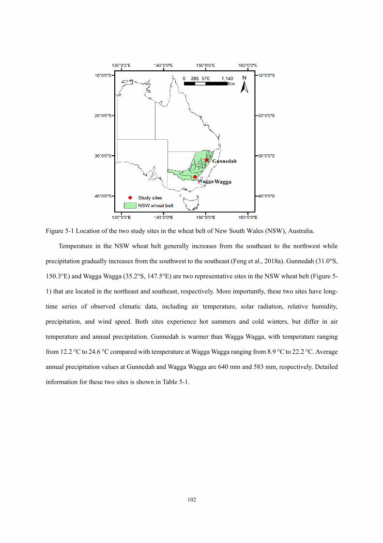
102

Figure 5-1 Location of the two study sites in the wheat belt of New South Wales (NSW), Australia.

Temperature in the NSW wheat belt generally increases from the southeast to the northwest while

precipitation gradually increases from the southwest to the southeast (Feng et al., 2018a). Gunnedah (31.0°S,

150.3°E) and Wagga Wagga (35.2°S, 147.5°E) are two representative sites in the NSW wheat belt (Figure 5-

1) that are located in the northeast and southeast, respectively. More importantly, these two sites have long-

time series of observed climatic data, including air temperature, solar radiation, relative humidity,

precipitation, and wind speed. Both sites experience hot summers and cold winters, but differ in air

temperature and annual precipitation. Gunnedah is warmer than Wagga Wagga, with temperature ranging

from 12.2 °C to 24.6 °C compared with temperature at Wagga Wagga ranging from 8.9 °C to 22.2 °C. Average

annual precipitation values at Gunnedah and Wagga Wagga are 640 mm and 583 mm, respectively. Detailed

information for these two sites is shown in Table 5-1.

Wagga

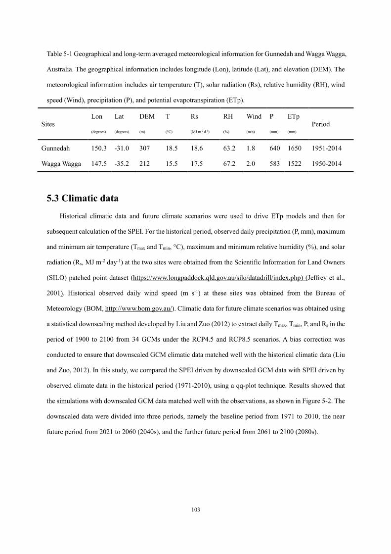
103

Table 5-1 Geographical and long-term averaged meteorological information for Gunnedah and Wagga Wagga,

Australia. The geographical information includes longitude (Lon), latitude (Lat), and elevation (DEM). The

meteorological information includes air temperature (T), solar radiation (Rs), relative humidity (RH), wind

speed (Wind), precipitation (P), and potential evapotranspiration (ETp).

Sites Lon

(degrees)

Lat

(degrees)

DEM

(m)

T

(°C)

Rs

(MJ m-2 d-1)

RH

(%)

Wind

(m/s)

P

(mm)

ETp

(mm) Period

Gunnedah 150.3 -31.0 307 18.5 18.6 63.2 1.8 640 1650 1951-2014

Wagga Wagga 147.5 -35.2 212 15.5 17.5 67.2 2.0 583 1522 1950-2014

5.3 Climatic data

Historical climatic data and future climate scenarios were used to drive ETp models and then for

subsequent calculation of the SPEI. For the historical period, observed daily precipitation (P, mm), maximum

and minimum air temperature (Tmax and Tmin, °C), maximum and minimum relative humidity (%), and solar

radiation (Rs, MJ m-2 day-1) at the two sites were obtained from the Scientific Information for Land Owners

(SILO) patched point dataset (https://www.longpaddock.qld.gov.au/silo/datadrill/index.php) (Jeffrey et al.,

2001). Historical observed daily wind speed (m s-1) at these sites was obtained from the Bureau of

Meteorology (BOM, http://www.bom.gov.au/). Climatic data for future climate scenarios was obtained using

a statistical downscaling method developed by Liu and Zuo (2012) to extract daily Tmax, Tmin, P, and Rs in the

period of 1900 to 2100 from 34 GCMs under the RCP4.5 and RCP8.5 scenarios. A bias correction was

conducted to ensure that downscaled GCM climatic data matched well with the historical climatic data (Liu

and Zuo, 2012). In this study, we compared the SPEI driven by downscaled GCM data with SPEI driven by

observed climate data in the historical period (1971-2010), using a qq-plot technique. Results showed that

the simulations with downscaled GCM data matched well with the observations, as shown in Figure 5-2. The

downscaled data were divided into three periods, namely the baseline period from 1971 to 2010, the near

future period from 2021 to 2060 (2040s), and the further future period from 2061 to 2100 (2080s).

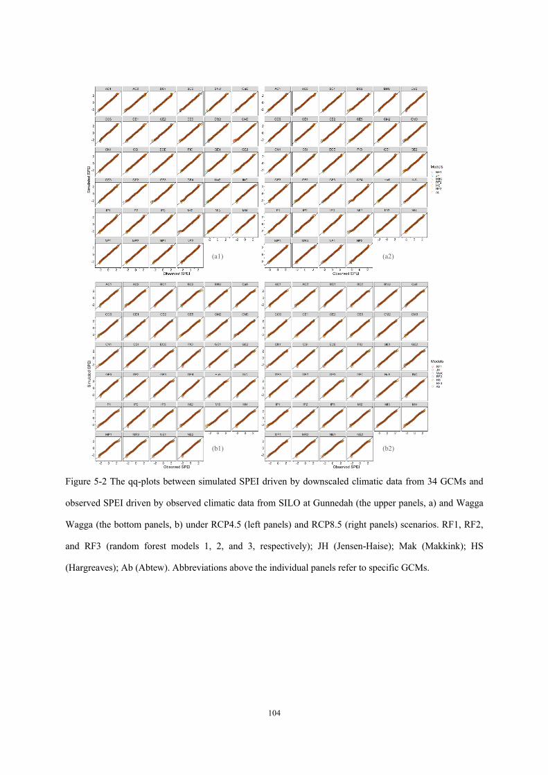
104

Figure 5-2 The qq-plots between simulated SPEI driven by downscaled climatic data from 34 GCMs and

observed SPEI driven by observed climatic data from SILO at Gunnedah (the upper panels, a) and Wagga

Wagga (the bottom panels, b) under RCP4.5 (left panels) and RCP8.5 (right panels) scenarios. RF1, RF2,

and RF3 (random forest models 1, 2, and 3, respectively); JH (Jensen-Haise); Mak (Makkink); HS

(Hargreaves); Ab (Abtew). Abbreviations above the individual panels refer to specific GCMs.

(a1) (a2)

(b1) (b2)

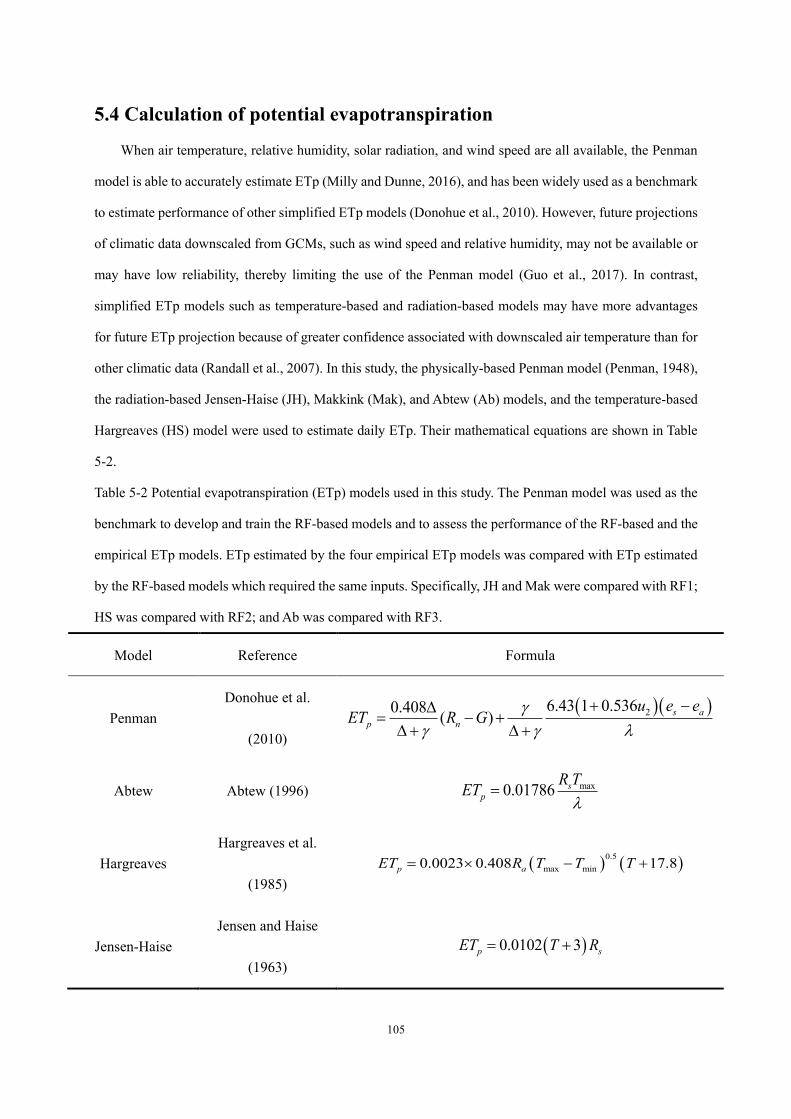
105

5.4 Calculation of potential evapotranspiration

When air temperature, relative humidity, solar radiation, and wind speed are all available, the Penman

model is able to accurately estimate ETp (Milly and Dunne, 2016), and has been widely used as a benchmark

to estimate performance of other simplified ETp models (Donohue et al., 2010). However, future projections

of climatic data downscaled from GCMs, such as wind speed and relative humidity, may not be available or

may have low reliability, thereby limiting the use of the Penman model (Guo et al., 2017). In contrast,

simplified ETp models such as temperature-based and radiation-based models may have more advantages

for future ETp projection because of greater confidence associated with downscaled air temperature than for

other climatic data (Randall et al., 2007). In this study, the physically-based Penman model (Penman, 1948),

the radiation-based Jensen-Haise (JH), Makkink (Mak), and Abtew (Ab) models, and the temperature-based

Hargreaves (HS) model were used to estimate daily ETp. Their mathematical equations are shown in Table

5-2.

Table 5-2 Potential evapotranspiration (ETp) models used in this study. The Penman model was used as the

benchmark to develop and train the RF-based models and to assess the performance of the RF-based and the

empirical ETp models. ETp estimated by the four empirical ETp models was compared with ETp estimated

by the RF-based models which required the same inputs. Specifically, JH and Mak were compared with RF1;

HS was compared with RF2; and Ab was compared with RF3.

Model Reference Formula

Penman Donohue et al.

(2010)

( )( )26.43 1 0.5360.408 ( ) s ap n

u e eET R G

+ −= − +

+ +

Abtew Abtew (1996) max0.01786 sp

R TET

=

Hargreaves Hargreaves et al.

(1985) ( ) ( )

0.5max min0.0023 0.408 17.8p aET R T T T= − +

Jensen-Haise Jensen and Haise

(1963) ( )0.0102 3p sET T R= +

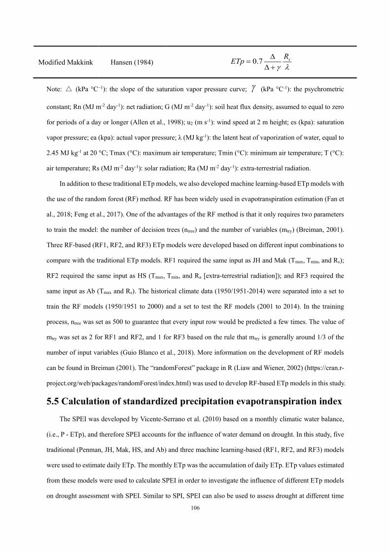
106

Modified Makkink Hansen (1984) 0.7 sRETp

=

+

Note: △ (kPa °C−1): the slope of the saturation vapor pressure curve; (kPa °C-1): the psychrometric

constant; Rn (MJ m-2 day-1): net radiation; G (MJ m-2 day-1): soil heat flux density, assumed to equal to zero

for periods of a day or longer (Allen et al., 1998); u2 (m s-1): wind speed at 2 m height; es (kpa): saturation

vapor pressure; ea (kpa): actual vapor pressure; λ (MJ kg-1): the latent heat of vaporization of water, equal to

2.45 MJ kg-1 at 20 °C; Tmax (°C): maximum air temperature; Tmin (°C): minimum air temperature; T (°C):

air temperature; Rs (MJ m-2 day-1): solar radiation; Ra (MJ m-2 day-1): extra-terrestrial radiation.

In addition to these traditional ETp models, we also developed machine learning-based ETp models with

the use of the random forest (RF) method. RF has been widely used in evapotranspiration estimation (Fan et

al., 2018; Feng et al., 2017). One of the advantages of the RF method is that it only requires two parameters

to train the model: the number of decision trees (ntree) and the number of variables (mtry) (Breiman, 2001).

Three RF-based (RF1, RF2, and RF3) ETp models were developed based on different input combinations to

compare with the traditional ETp models. RF1 required the same input as JH and Mak (Tmax, Tmin, and Rs);

RF2 required the same input as HS (Tmax, Tmin, and Ra [extra-terrestrial radiation]); and RF3 required the

same input as Ab (Tmax and Rs). The historical climate data (1950/1951-2014) were separated into a set to

train the RF models (1950/1951 to 2000) and a set to test the RF models (2001 to 2014). In the training

process, ntree was set as 500 to guarantee that every input row would be predicted a few times. The value of

mtry was set as 2 for RF1 and RF2, and 1 for RF3 based on the rule that mtry is generally around 1/3 of the

number of input variables (Guio Blanco et al., 2018). More information on the development of RF models

can be found in Breiman (2001). The “randomForest” package in R (Liaw and Wiener, 2002) (https://cran.r-

project.org/web/packages/randomForest/index.html) was used to develop RF-based ETp models in this study.

5.5 Calculation of standardized precipitation evapotranspiration index

The SPEI was developed by Vicente-Serrano et al. (2010) based on a monthly climatic water balance,

(i.e., P - ETp), and therefore SPEI accounts for the influence of water demand on drought. In this study, five

traditional (Penman, JH, Mak, HS, and Ab) and three machine learning-based (RF1, RF2, and RF3) models

were used to estimate daily ETp. The monthly ETp was the accumulation of daily ETp. ETp values estimated

from these models were used to calculate SPEI in order to investigate the influence of different ETp models

on drought assessment with SPEI. Similar to SPI, SPEI can also be used to assess drought at different time

107

scales (Potop et al., 2012). Three months with P-ETp significantly lower than the normal level will generally

result in a decrease in soil moisture, thus leading to crop failure and the occurrence of agricultural drought

(Vicente-Serrano et al., 2011). Therefore, a 3-month SPEI can describe soil water conditions during crop

growing seasons. In this study, a 3-month time period was used to calculate seasonal SPEI based on the

accumulated monthly water balance. For instance, spring SPEI was based on the accumulated water balance

from September to November while summer SPEI was based on the accumulated water balance from

December to February.

In specific, the calculation of SPEI is described as following:

(1) Calculation of monthly water balance:

j j jD P ETp= − (5-1)

where, Pj (mm) and ETpj (mm) are the total precipitation and ETp of the j-th month, respectively.

(2) Calculation of the 3-month accumulated water balance for seasonal SPEI calculation

123, 1, ,

10 1

3, ,

2

3

3

j

i j i l i ll j l

j

i j i ll j

X D D if j

X D if j

−

= + =

= −

= +

=

(5-2)

where 𝑋𝑖,𝑗3 is the 3-month accumulated water balance in the j-th month of the i-th year; in this study, j is in

11 (November for spring), 2 (February for summer), 5 (May for autumn), and 8 (August for winter). 𝐷𝑖,𝑙 is

the monthly water balance in the l-th month of i-th year.

(3) Normalize the 𝑋𝑖,𝑗3 data sequence with the three-parameter log-logistic probability distribution

recommended by Vicente-Serrano et al. (2010). The accumulative function of the log-logistic probability

distribution F(X) is expressed as:

( )

1

1F XX

−

= +

−

(5-3)

where 𝛼,  𝛽,and 𝛾 are scale, shape, and position parameters, respectively. They could be calculated with

equations suggested by Vicente-Serrano et al. (2010).

p is the probability of a definite 𝑋𝑖,𝑗3 value:

( )1p F X= − (5-4),

if p ≤ 0.5, 2lnw p= − , 2

0 1 22 3

1 2 31C C w C wSPEI wd w d w d w+ +

= −+ + +

,

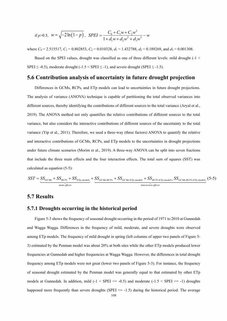
108

if p>0.5, ( )2ln 1w p= − − , 2

0 1 22 3

1 2 31C C w C wSPEI wd w d w d w+ +

= −+ + +

where C0 = 2.515517, C1 = 0.802853, C2 = 0.010328, d1 = 1.432788, d2 = 0.189269, and d3 = 0.001308.

Based on the SPEI values, drought was classified as one of three different levels: mild drought (-1 <

SPEI ≤ -0.5), moderate drought (-1.5 < SPEI ≤ -1), and severe drought (SPEI ≤ -1.5).

5.6 Contribution analysis of uncertainty in future drought projection

Differences in GCMs, RCPs, and ETp models can lead to uncertainties in future drought projections.

The analysis of variance (ANOVA) technique is capable of partitioning the total observed variances into

different sources, thereby identifying the contributions of different sources to the total variance (Aryal et al.,

2019). The ANOVA method not only quantifies the relative contributions of different sources to the total

variance, but also considers the interactive contributions of different sources of the uncertainty to the total

variance (Yip et al., 2011). Therefore, we used a three-way (three factors) ANOVA to quantify the relative

and interactive contributions of GCMs, RCPs, and ETp models to the uncertainties in drought projections

under future climate scenarios (Morim et al., 2019). A three-way ANOVA can be split into seven fractions

that include the three main effects and the four interaction effects. The total sum of squares (SST) was

calculated as equation (5-5):

, : : , : , : : , (5-5)GCMs RCPs ETp models GCMs RCPs GCMs ETp models RCPs ETp models GCMs RCPs ETp models

main effects interaction effects

SST SS SS SS SS SS SS SS+= + + + + +

5.7 Results

5.7.1 Droughts occurring in the historical period

Figure 5-3 shows the frequency of seasonal drought occurring in the period of 1971 to 2010 at Gunnedah

and Wagga Wagga. Differences in the frequency of mild, moderate, and severe droughts were observed

among ETp models. The frequency of mild drought in spring (left columns of upper two panels of Figure 5-

3) estimated by the Penman model was about 20% at both sites while the other ETp models produced lower

frequencies at Gunnedah and higher frequencies at Wagga Wagga. However, the differences in total drought

frequency among ETp models were not great (lower two panels of Figure 5-3). For instance, the frequency

of seasonal drought estimated by the Penman model was generally equal to that estimated by other ETp

models at Gunnedah. In addition, mild (-1 < SPEI <= -0.5) and moderate (-1.5 < SPEI <= -1) droughts

happened more frequently than severe droughts (SPEI <= -1.5) during the historical period. The average

109

frequency of mild drought at Gunnedah ranged from 9% (in winter) to 20% (in spring) while the

corresponding values for severe drought ranged from 2% (in summer) to 6% (in spring).

Figure 5-3 Frequency of seasonal droughts occurring in the period from 1971 to 2010 at Gunnedah and

Wagga Wagga, Australia, using eight potential evapotranspiration models. RF1, RF2, and RF3 (random

forest models 1, 2, and 3, respectively); JH (Jensen-Haise); Mak (Makkink); HS (Hargreaves); Ab (Abtew).

Mild, moderate, and severe drought classifications are based on Standardized Precipitation

Evapotranspiration Index values as described in section 5.5. Drought refers to the total of all drought

classifications.

Differences in ETp estimated by different models are shown in Figure5-4. The RF-based ETp models

generally produced similar values as the Penman model. In contrast, the other ETp models generally produced

smaller ETp values. However, the underestimated seasonal ETp did not always produce less drought

occurrence. This may indicate that drought assessment was mainly dominated by precipitation while ETp

played only a minor role in the historical period.

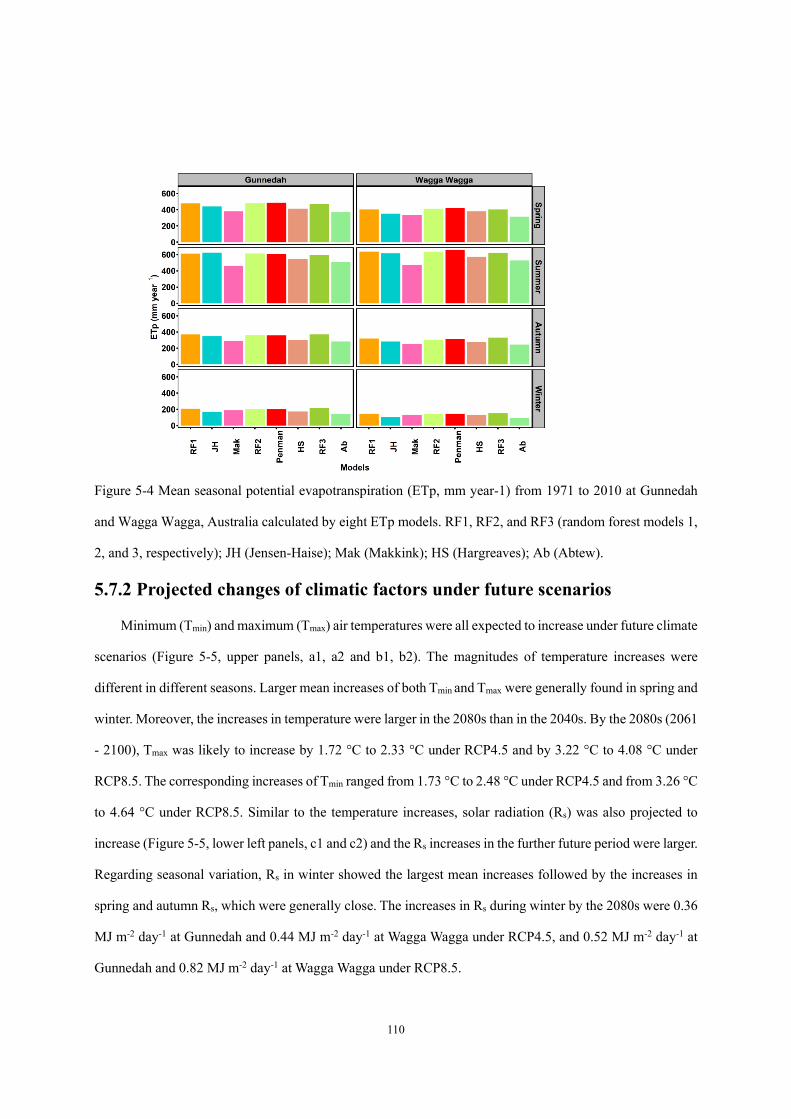
110

Figure 5-4 Mean seasonal potential evapotranspiration (ETp, mm year-1) from 1971 to 2010 at Gunnedah

and Wagga Wagga, Australia calculated by eight ETp models. RF1, RF2, and RF3 (random forest models 1,

2, and 3, respectively); JH (Jensen-Haise); Mak (Makkink); HS (Hargreaves); Ab (Abtew).

5.7.2 Projected changes of climatic factors under future scenarios

Minimum (Tmin) and maximum (Tmax) air temperatures were all expected to increase under future climate

scenarios (Figure 5-5, upper panels, a1, a2 and b1, b2). The magnitudes of temperature increases were

different in different seasons. Larger mean increases of both Tmin and Tmax were generally found in spring and

winter. Moreover, the increases in temperature were larger in the 2080s than in the 2040s. By the 2080s (2061

- 2100), Tmax was likely to increase by 1.72 °C to 2.33 °C under RCP4.5 and by 3.22 °C to 4.08 °C under

RCP8.5. The corresponding increases of Tmin ranged from 1.73 °C to 2.48 °C under RCP4.5 and from 3.26 °C

to 4.64 °C under RCP8.5. Similar to the temperature increases, solar radiation (Rs) was also projected to

increase (Figure 5-5, lower left panels, c1 and c2) and the Rs increases in the further future period were larger.

Regarding seasonal variation, Rs in winter showed the largest mean increases followed by the increases in

spring and autumn Rs, which were generally close. The increases in Rs during winter by the 2080s were 0.36

MJ m-2 day-1 at Gunnedah and 0.44 MJ m-2 day-1 at Wagga Wagga under RCP4.5, and 0.52 MJ m-2 day-1 at

Gunnedah and 0.82 MJ m-2 day-1 at Wagga Wagga under RCP8.5.

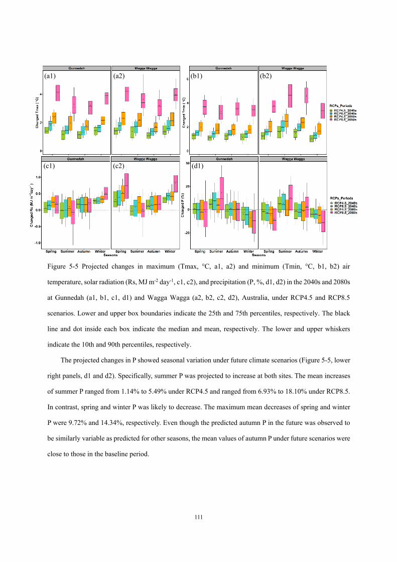
111

Figure 5-5 Projected changes in maximum (Tmax, °C, a1, a2) and minimum (Tmin, °C, b1, b2) air

temperature, solar radiation (Rs, MJ m-2 day-1, c1, c2), and precipitation (P, %, d1, d2) in the 2040s and 2080s

at Gunnedah (a1, b1, c1, d1) and Wagga Wagga (a2, b2, c2, d2), Australia, under RCP4.5 and RCP8.5

scenarios. Lower and upper box boundaries indicate the 25th and 75th percentiles, respectively. The black

line and dot inside each box indicate the median and mean, respectively. The lower and upper whiskers

indicate the 10th and 90th percentiles, respectively.

The projected changes in P showed seasonal variation under future climate scenarios (Figure 5-5, lower

right panels, d1 and d2). Specifically, summer P was projected to increase at both sites. The mean increases

of summer P ranged from 1.14% to 5.49% under RCP4.5 and ranged from 6.93% to 18.10% under RCP8.5.

In contrast, spring and winter P was likely to decrease. The maximum mean decreases of spring and winter

P were 9.72% and 14.34%, respectively. Even though the predicted autumn P in the future was observed to

be similarly variable as predicted for other seasons, the mean values of autumn P under future scenarios were

close to those in the baseline period.

(a1) (a2) (b1) (b2)

(c1) (c2) (d1)

112

5.7.3 Projected changes of potential evapotranspiration under future climate

scenarios

ETp projected by all models was likely to increase under future climate scenarios, although the

magnitudes of increase varied among models (Figure 5-6). In general, RF-based models (followed by JH and

Ab) produced larger ETp increases, whereas Mak and HS yielded smaller increases. Moreover, the ETp

increases showed similar seasonal variation with that of temperatures, i.e., larger increases were generally

observed in spring and winter, whereas smaller increases were observed in summer and autumn. By the 2080s

(2061 - 2100), the mean increases in spring ETp ranged from 4.6% to 15.6% under RCP4.5 and from 7.7%

to 26.9% under RCP8.5; the mean summer ETp values were likely to increase by 2.9% to 10.1% under

RCP4.5 and by 3.5% to 16.1% under RCP8.5; in autumn, the projected increase of mean ETp ranged from

2.9% to 11.2% under RCP4.5 and from 3.6% to 22.7% under RCP8.5; and the likely increases in mean winter

ETp ranged from 7.5% to 23.3% and 13.1% to 44.0% under RCP4.5 and RCP8.5, respectively. Results of

the multiple linear regression (Figure 5-7, ΔETp (%) = a0*ΔTmax (°C) + b0*ΔTmin (°C) + c0*ΔRs (MJ m-

2 day-1)) showed that changes in ETp could be almost entirely explained by changes in Tmax, Tmin, and Rs.

However, the sensitivity of ETp models to these climatic factors varied. In general, models requiring the

same inputs showed similar sensitivity to the same climatic factors. For instance, ETp estimated by RF1, JH,

and Mak was more sensitive to changes in Rs than to changes in Tmax or Tmin. In contrast, a unit increase

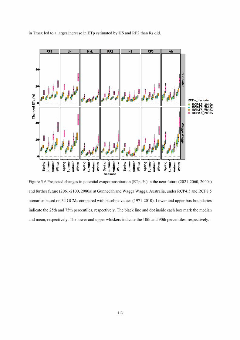
113

in Tmax led to a larger increase in ETp estimated by HS and RF2 than Rs did.

Figure 5-6 Projected changes in potential evapotranspiration (ETp, %) in the near future (2021-2060, 2040s)

and further future (2061-2100, 2080s) at Gunnedah and Wagga Wagga, Australia, under RCP4.5 and RCP8.5

scenarios based on 34 GCMs compared with baseline values (1971-2010). Lower and upper box boundaries

indicate the 25th and 75th percentiles, respectively. The black line and dot inside each box mark the median

and mean, respectively. The lower and upper whiskers indicate the 10th and 90th percentiles, respectively.

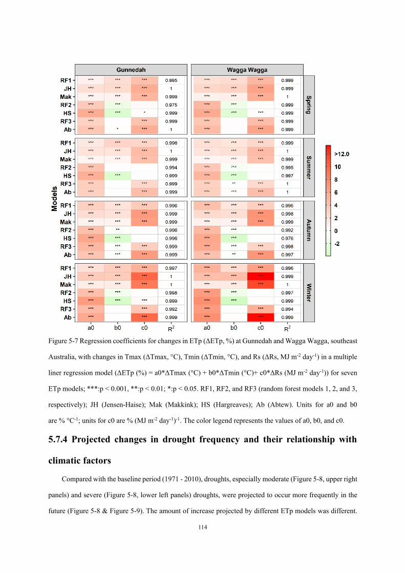
114

Figure 5-7 Regression coefficients for changes in ETp (ΔETp, %) at Gunnedah and Wagga Wagga, southeast

Australia, with changes in Tmax (ΔTmax, °C), Tmin (ΔTmin, °C), and Rs (ΔRs, MJ m-2 day-1) in a multiple

liner regression model (ΔETp (%) = a0*ΔTmax (°C) + b0*ΔTmin (°C)+ c0*ΔRs (MJ m-2 day-1)) for seven

ETp models; ***:p < 0.001, **:p < 0.01; *:p < 0.05. RF1, RF2, and RF3 (random forest models 1, 2, and 3,

respectively); JH (Jensen-Haise); Mak (Makkink); HS (Hargreaves); Ab (Abtew). Units for a0 and b0

are % °C-1; units for c0 are % (MJ m-2 day-1)-1. The color legend represents the values of a0, b0, and c0.

5.7.4 Projected changes in drought frequency and their relationship with

climatic factors

Compared with the baseline period (1971 - 2010), droughts, especially moderate (Figure 5-8, upper right

panels) and severe (Figure 5-8, lower left panels) droughts, were projected to occur more frequently in the

future (Figure 5-8 & Figure 5-9). The amount of increase projected by different ETp models was different.

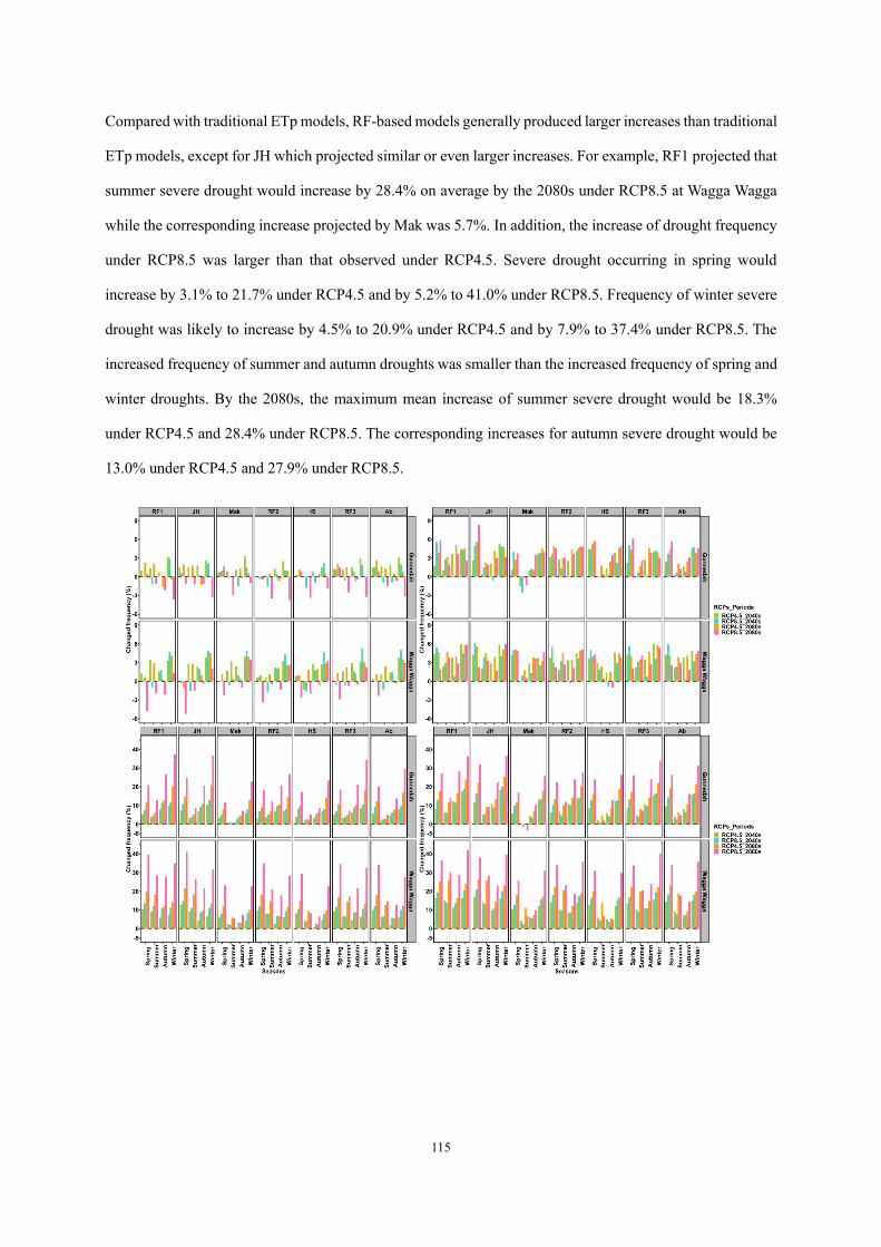
115

Compared with traditional ETp models, RF-based models generally produced larger increases than traditional

ETp models, except for JH which projected similar or even larger increases. For example, RF1 projected that

summer severe drought would increase by 28.4% on average by the 2080s under RCP8.5 at Wagga Wagga

while the corresponding increase projected by Mak was 5.7%. In addition, the increase of drought frequency

under RCP8.5 was larger than that observed under RCP4.5. Severe drought occurring in spring would

increase by 3.1% to 21.7% under RCP4.5 and by 5.2% to 41.0% under RCP8.5. Frequency of winter severe

drought was likely to increase by 4.5% to 20.9% under RCP4.5 and by 7.9% to 37.4% under RCP8.5. The

increased frequency of summer and autumn droughts was smaller than the increased frequency of spring and

winter droughts. By the 2080s, the maximum mean increase of summer severe drought would be 18.3%

under RCP4.5 and 28.4% under RCP8.5. The corresponding increases for autumn severe drought would be

13.0% under RCP4.5 and 27.9% under RCP8.5.

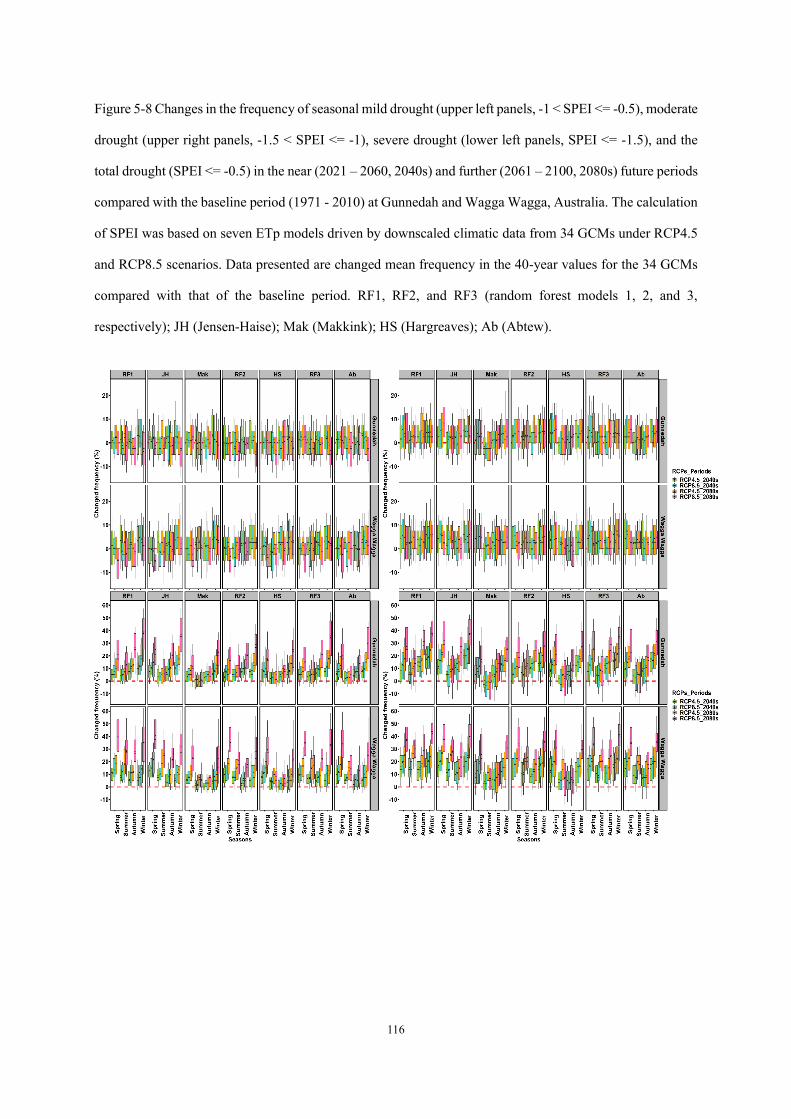
116

Figure 5-8 Changes in the frequency of seasonal mild drought (upper left panels, -1 < SPEI <= -0.5), moderate

drought (upper right panels, -1.5 < SPEI <= -1), severe drought (lower left panels, SPEI <= -1.5), and the

total drought (SPEI <= -0.5) in the near (2021 – 2060, 2040s) and further (2061 – 2100, 2080s) future periods

compared with the baseline period (1971 - 2010) at Gunnedah and Wagga Wagga, Australia. The calculation

of SPEI was based on seven ETp models driven by downscaled climatic data from 34 GCMs under RCP4.5

and RCP8.5 scenarios. Data presented are changed mean frequency in the 40-year values for the 34 GCMs

compared with that of the baseline period. RF1, RF2, and RF3 (random forest models 1, 2, and 3,

respectively); JH (Jensen-Haise); Mak (Makkink); HS (Hargreaves); Ab (Abtew).

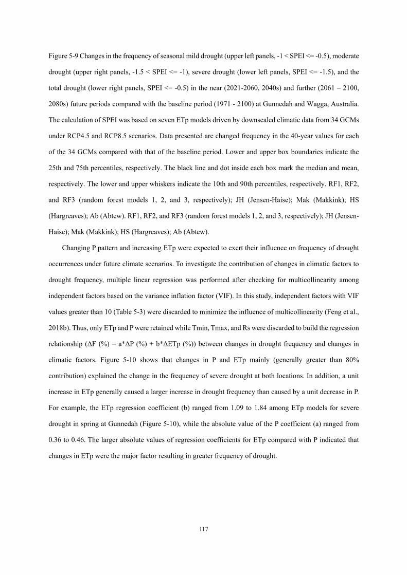
117

Figure 5-9 Changes in the frequency of seasonal mild drought (upper left panels, -1 < SPEI <= -0.5), moderate

drought (upper right panels, -1.5 < SPEI <= -1), severe drought (lower left panels, SPEI <= -1.5), and the

total drought (lower right panels, SPEI <= -0.5) in the near (2021-2060, 2040s) and further (2061 – 2100,

2080s) future periods compared with the baseline period (1971 - 2100) at Gunnedah and Wagga, Australia.

The calculation of SPEI was based on seven ETp models driven by downscaled climatic data from 34 GCMs

under RCP4.5 and RCP8.5 scenarios. Data presented are changed frequency in the 40-year values for each

of the 34 GCMs compared with that of the baseline period. Lower and upper box boundaries indicate the

25th and 75th percentiles, respectively. The black line and dot inside each box mark the median and mean,

respectively. The lower and upper whiskers indicate the 10th and 90th percentiles, respectively. RF1, RF2,

and RF3 (random forest models 1, 2, and 3, respectively); JH (Jensen-Haise); Mak (Makkink); HS

(Hargreaves); Ab (Abtew). RF1, RF2, and RF3 (random forest models 1, 2, and 3, respectively); JH (Jensen-

Haise); Mak (Makkink); HS (Hargreaves); Ab (Abtew).

Changing P pattern and increasing ETp were expected to exert their influence on frequency of drought

occurrences under future climate scenarios. To investigate the contribution of changes in climatic factors to

drought frequency, multiple linear regression was performed after checking for multicollinearity among

independent factors based on the variance inflation factor (VIF). In this study, independent factors with VIF

values greater than 10 (Table 5-3) were discarded to minimize the influence of multicollinearity (Feng et al.,

2018b). Thus, only ETp and P were retained while Tmin, Tmax, and Rs were discarded to build the regression

relationship (ΔF (%) = a*ΔP (%) + b*ΔETp (%)) between changes in drought frequency and changes in

climatic factors. Figure 5-10 shows that changes in P and ETp mainly (generally greater than 80%

contribution) explained the change in the frequency of severe drought at both locations. In addition, a unit

increase in ETp generally caused a larger increase in drought frequency than caused by a unit decrease in P.

For example, the ETp regression coefficient (b) ranged from 1.09 to 1.84 among ETp models for severe

drought in spring at Gunnedah (Figure 5-10), while the absolute value of the P coefficient (a) ranged from

0.36 to 0.46. The larger absolute values of regression coefficients for ETp compared with P indicated that

changes in ETp were the major factor resulting in greater frequency of drought.

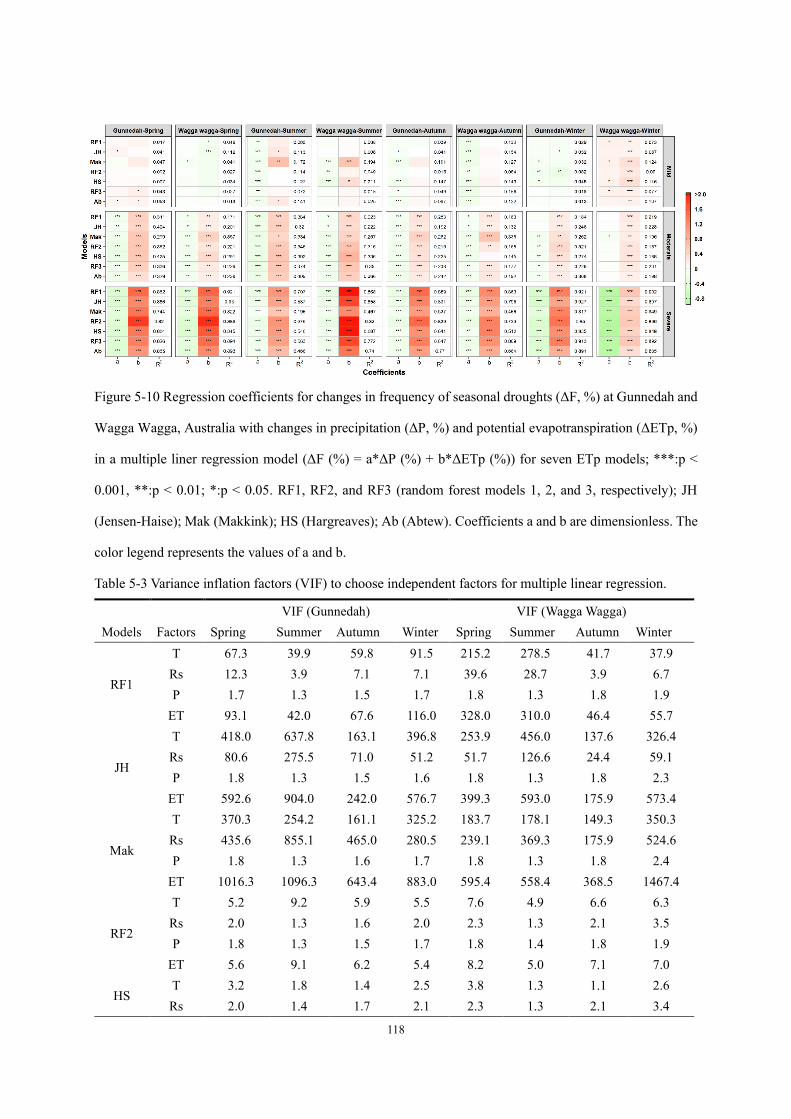
118

Figure 5-10 Regression coefficients for changes in frequency of seasonal droughts (ΔF, %) at Gunnedah and

Wagga Wagga, Australia with changes in precipitation (ΔP, %) and potential evapotranspiration (ΔETp, %)

in a multiple liner regression model (ΔF (%) = a*ΔP (%) + b*ΔETp (%)) for seven ETp models; ***:p <

0.001, **:p < 0.01; *:p < 0.05. RF1, RF2, and RF3 (random forest models 1, 2, and 3, respectively); JH

(Jensen-Haise); Mak (Makkink); HS (Hargreaves); Ab (Abtew). Coefficients a and b are dimensionless. The

color legend represents the values of a and b.

Table 5-3 Variance inflation factors (VIF) to choose independent factors for multiple linear regression.

VIF (Gunnedah) VIF (Wagga Wagga) Models Factors Spring Summer Autumn Winter Spring Summer Autumn Winter

RF1

T 67.3 39.9 59.8 91.5 215.2 278.5 41.7 37.9 Rs 12.3 3.9 7.1 7.1 39.6 28.7 3.9 6.7 P 1.7 1.3 1.5 1.7 1.8 1.3 1.8 1.9

ET 93.1 42.0 67.6 116.0 328.0 310.0 46.4 55.7

JH

T 418.0 637.8 163.1 396.8 253.9 456.0 137.6 326.4 Rs 80.6 275.5 71.0 51.2 51.7 126.6 24.4 59.1 P 1.8 1.3 1.5 1.6 1.8 1.3 1.8 2.3

ET 592.6 904.0 242.0 576.7 399.3 593.0 175.9 573.4

Mak

T 370.3 254.2 161.1 325.2 183.7 178.1 149.3 350.3 Rs 435.6 855.1 465.0 280.5 239.1 369.3 175.9 524.6 P 1.8 1.3 1.6 1.7 1.8 1.3 1.8 2.4

ET 1016.3 1096.3 643.4 883.0 595.4 558.4 368.5 1467.4

RF2

T 5.2 9.2 5.9 5.5 7.6 4.9 6.6 6.3 Rs 2.0 1.3 1.6 2.0 2.3 1.3 2.1 3.5 P 1.8 1.3 1.5 1.7 1.8 1.4 1.8 1.9

ET 5.6 9.1 6.2 5.4 8.2 5.0 7.1 7.0

HS T 3.2 1.8 1.4 2.5 3.8 1.3 1.1 2.6 Rs 2.0 1.4 1.7 2.1 2.3 1.3 2.1 3.4

119

P 1.8 1.3 1.5 1.7 1.8 1.4 1.8 1.9 ET 3.5 1.8 1.7 2.4 4.3 1.2 1.3 2.4

RF3

T 22.3 9.4 7.2 12.0 22.1 10.4 7.7 9.8 Rs 7.9 3.6 2.9 2.6 8.5 3.4 2.7 4.5 P 1.8 1.3 1.5 1.7 1.8 1.4 1.8 1.9

ET 33.2 11.6 8.8 15.1 37.5 12.6 9.2 14.6

Ab

T 25.4 9.4 7.0 12.3 23.3 10.8 7.0 12.0 Rs 10.2 7.1 6.7 4.1 11.0 7.3 5.6 7.6 P 1.8 1.3 1.5 1.7 1.8 1.4 1.8 2.0

ET 39.7 15.0 12.6 19.3 43.4 17.0 11.9 25.8

5.7.5 Uncertainty analysis in drought projection

The contributions of different sources of variation and their interactions to the total uncertainty in

projecting drought frequency are shown in Figure 5-11. GCMs and their interaction with RCPs (GCMs:RCPs)

contributed the most to the total uncertainty independent of drought level, season, and site. The uncertainty

contribution of GCMs and GCMs:RCPs ranged from 19.2% to 53.0% and from 17.2% to 44.3%, respectively.

The contribution of RCPs to severe drought and the interaction of GCMs, RCPs, and ETp models

(GCMs:RCPs:Models) to mild and moderate droughts were also large. In contrast, the contribution of ETp

models to the total uncertainty was negligible, generally less than 5.0%. The results of this uncertainty

analysis indicated that the projection of drought under future climate was only slightly influenced by the

differences in ETp models, but greatly influenced by GCMs and RCPs.

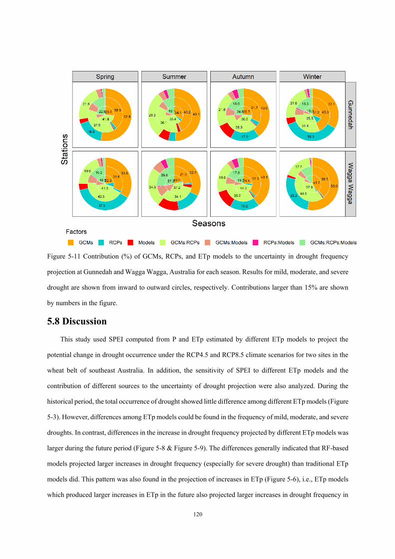
120

Figure 5-11 Contribution (%) of GCMs, RCPs, and ETp models to the uncertainty in drought frequency

projection at Gunnedah and Wagga Wagga, Australia for each season. Results for mild, moderate, and severe

drought are shown from inward to outward circles, respectively. Contributions larger than 15% are shown

by numbers in the figure.

5.8 Discussion

This study used SPEI computed from P and ETp estimated by different ETp models to project the

potential change in drought occurrence under the RCP4.5 and RCP8.5 climate scenarios for two sites in the

wheat belt of southeast Australia. In addition, the sensitivity of SPEI to different ETp models and the

contribution of different sources to the uncertainty of drought projection were also analyzed. During the

historical period, the total occurrence of drought showed little difference among different ETp models (Figure

5-3). However, differences among ETp models could be found in the frequency of mild, moderate, and severe

droughts. In contrast, differences in the increase in drought frequency projected by different ETp models was

larger during the future period (Figure 5-8 & Figure 5-9). The differences generally indicated that RF-based

models projected larger increases in drought frequency (especially for severe drought) than traditional ETp

models did. This pattern was also found in the projection of increases in ETp (Figure 5-6), i.e., ETp models

which produced larger increases in ETp in the future also projected larger increases in drought frequency in

121

the future. Yao et al. (2019) assessed the influence of different ETp models on drought monitoring in China

with the use of SPEI. They concluded that the accuracy of ETp models played only a minor role in drought

assessments at wetter sites where P was greater than 500 mm year -1, while ETp models made a large

difference in drought assessment at drier sites. The mean historical annual P at our study sites was slightly

greater than 500 mm, but it was projected to decrease (Figure 5-5, d1 and d2) under future climate scenarios.

This can explain why the influence of different ETp models on drought projection was greater in the future

periods. Additionally, other studies (Asadi Zarch et al., 2017; Asadi Zarch et al., 2015; Cook et al., 2014)

have shown that ETp was more important to future drought projection than to historical drought assessment.

For instance, Asadi Zarch et al. (2015) used both SPI (based only on P) and RDI (based on ETp and P) to

assess changes in global drought. They found that there was a significant agreement in drought assessment

between SPI and RDI only in historical periods. However, a significant difference was observed in future

drought projection between the two methods, and RDI projected more occurrences of drought in the future

than SPI did. They stated that “agreement between SPI and RDI is affected and decreases remarkably over

time”. Therefore, it is necessary to include ETp in future drought projection studies and attention should also

be given to ETp model use.

Increases in drought frequency at Wagga Wagga were generally larger than those observed at Gunnedah

(Figure 5-8). This may be explained by the greater increases in temperature and solar radiation at Wagga

Wagga. Additionally, precipitation is likely to be somewhat less at Wagga Wagga than at Gunnedah in the

future (Figure 5-5, d1 and d2). During the historical period, Wagga Wagga was also slightly drier than

Gunnedah. Thus, the greater increase in drought is likely to present greater challenges to agricultural

production at this site. In addition to the increase in future drought projected by offline indices, direct GCM

outputs, such as soil moisture and runoff, have also supported the increase in future drought on a large scale

(Zhang et al., 2018; Zhao and Dai, 2015; Zhao and Dai, 2017). For instance, Zhao and Dai (2015) used

sc_PDSI, soil moisture in the 0-10 cm surface soil layer, and runoff from 14 GCMs to project drought under

the RCP4.5 scenario at global scale. They found that all of these measures projected increases in drought

over most land areas. Although general increases have been widely reported across the world, the magnitudes

of the increases have varied among studies (Dai, 2012; Dai and Zhao, 2017; Milly and Dunne, 2016;

Naumann et al., 2018). Based on 12-month SPEI with the Penman-Monteith model, Naumann et al. (2018)

projected that drought magnitudes could double for 30% of the global landmass with 1.5 °C warming.

Meanwhile, they found that water supply-demand deficit could increase by fivefold for Australia if

122

contemporary warming rates continue. However, Milly and Dunne (2016) reported that ETp-dependent

metrics may overpredict drought increases. Similarly, Yang et al. (2018) found that regardless of the obvious

drying atmosphere trend for the 21st century, surface runoff was likely to increase across most of the global

land area. In our study, the increases in drought varied greatly depending on seasons, ETp models, and climate

scenarios (Figure 5-8). The discrepancies among these studies demonstrate the need for further research

studies in drought projection. The discrepancies also indicate that drought projection is partially influenced

by drought definition and the indices used. The results of our study provide a substantial contribution to the

debate on the effect of different ETp models on drought quantification.

According to our study, more frequent and severe drought under future climate scenarios was generally

the result of a combined effect of increasing ETp and decreasing P (Figure 5-10) and the increase of ETp

might play a major role in the increase of drought in the future period. Similar to our study, Cook et al. (2014)

also found that declines in P would push the climate towards drought while the increased ETp would amplify

the precipitation-induced drought. The projected increase in drought occurrence will inevitably lead to

decreased crop yields and cause more challenges to cropping systems (Dijk et al., 2013; Lobell et al., 2015).

Because spring and winter are key growing seasons for wheat and canola (Brassica napus L.) in this region

of Australia and because these crops are mainly grown under rainfed conditions, they will be more vulnerable

to drought-induced yield losses in the future (Feng et al., 2020; Luo et al., 2005). Thus, measures should be

taken to minimize the negative influence of droughts. Breeding new crop varieties that have greater drought

tolerance, use of irrigation, and changing planting date are three possible measures that could mitigate

drought-induced yield loss (Chenu et al., 2011; Watson et al., 2017).

This study found that differences in GCMs and their interaction with RCPs (GCMs:RCPs) contributed

the most to the uncertainty in the process of drought projection (19.2% - 53% and 17.2% - 44.3%, respectively;

Figure 5-11). Lu et al. (2019) found that differences in GCMs could account for more than 80% of the

uncertainty in drought projection based on soil moisture anomalies. The large contribution of GCMs might

be due to the differences in P projected by different GCMs. For instance, Hawkins and Sutton (2011) found

that GCMs generally played a dominant role among GCMs, RCPs, and the random, internal variations in

climate with regard to the uncertainty of P projection for lead times longer than 30 years. Different RCPs

generally resulted in different temperature predictions, which would influence ETp prediction. Shi et al.

(2020) found that RCP differences could explain around 40% of the uncertainty in ETp projection. This may

explain why the GCMs:RCPs interaction also played a key role in the uncertainty of drought projection in

123

our study. The dominant contribution of GCMs and GCMs:RCPs to drought assessment highlighted the

importance of using a wide range of GCMs and different emission scenarios to avoid the underestimation of

the total uncertainty. For policymakers, the less uncertainty that there is in drought projections, the more

reliable are the measures that can be recommended. Therefore, the possibility of reducing uncertainty in

drought projection should be investigated in the future. The availability of more and more GCMs from

CMIP6 might provide the possibility of reducing such uncertainty through the consideration of more

environmental factors, the use of more advanced numerical simulation methods, and the generally higher

resolution (Eyring et al., 2016).

A few limitations in our study should be acknowledged. In addition to SPEI, there are other drought

indices such as RDI (Tsakiris et al., 2007), and their sensitivity to different ETp models was not reported in

this study. Therefore, more drought indices should be included in future studies to better understand the

comprehensive influence of evapotranspiration on drought. In addition, the influence of enriched CO2

environment on drought projection is complex (Berdugo et al., 2020; Vicente-Serrano et al., 2019). There

were two reasons for why we did not consider CO2 fertilization in our study. First, we used the open-water

Penman model rather than the reference crop Penman-Monteith model to calculate ETp instead of ET0 or

actual evapotranspiration. Second, increasing atmospheric CO2 concentration is expected to influence plant

structure (e.g., leaf size, root length), and function (e.g., stomatal resistance, vegetation evapotranspiration)

(Pritchard et al., 1999; Yang et al., 2019). Thus, the effects of enriched CO2 on drought projection should

ideally involve a consideration of other biophysical factors such as plant development and their response to

the changing meteorological factors (Sheffield et al., 2012). The biophysical modelling component was not

considered in our study. Recently, Yang et al. (2019) modified the Penman-Monteith model by adding a

trained relationship between CO2 and surface resistance to consider the influence of elevated CO2 on ET0.

They adopted the modified and the original Penman-Monteith model, and direct outputs from 16 GCMs to

project global drought under RCP8.5 based on PDSI, and observed that the degree of increase in drought was

much smaller with the modified Penman-Monteith model because the elevated CO2 offset the ET0 increase

caused by increased temperature (Yang et al., 2020). Their study sets an example for future studies to

comprehensively assess the influence of climate change on drought with consideration of plant response to

elevated CO2. However, elevated CO2 will not only lead to partial stomatal closure (reducing

evapotranspiration,) but will also lead to larger leaf size (Pritchard et al., 1999) (increasing

evapotranspiration). Additionally, as Berdugo et al. (2020) reported in their response to Keenan et al. (2020),

124

the positive effect of CO2 fertilization on vegetation growth and evapotranspiration may be dampened or

even reversed by the effects of increased soil temperature, continued drying, and extreme climatic events in

the future. In this context, there is a need to consider other important factors when exploring the impacts of

climate change and CO2 fertilization on future drought.

5.9 Conclusions

This study used SPEI to project possible changes of drought under two different emission scenarios

(RCP4.5 and RCP8.5) for two locations in the wheat belt of southeastern Australia based on climate data

downscaled from 34 GCMs. Three newly developed random forest (RF1, RF2, and RF3) models and five

traditional potential evapotranspiration (ETp) models were used to calculate SPEI to investigate the influence

of ETp models on drought assessment. The influence of ETp models on drought assessment with SPEI was

evident for future periods even though little difference was observed among these ETp models in the

historical drought assessment period. Generally, RF-based ETp models which projected larger increases in

ETp also projected larger increases in drought frequency. This finding emphasized the necessity of using

drought indices which include both P and ETp to predict drought under a changing climate. A greater increase

in frequency of moderate and severe droughts was predicted than for mild droughts. The increased occurrence

of droughts showed seasonal variations, with larger increases in spring and winter and smaller increases in

autumn and winter. For instance, the maximum mean increase of frequency of severe drought in spring was

21.7% under RCP45 and 41.0% under RCP85 by the 2080s, while the corresponding increase for autumn

severe drought was 13.0% under RCP4.5 and 27.9% under RCP8.5. The projection of droughts under future

climate scenarios was accompanied by uncertainties. Our study showed that the uncertainty was mainly due

to differences in GCMs (19.2% - 53%) followed by the interaction of GCMs with RCPs. Despite the

uncertainty, results from our study highlight the necessity of identifying mitigation and adaptation strategies

to deal with the potential negative impacts caused by more moderate and severe droughts in the future.

125

5.10 Reference Abtew, W., 1996. Evapotranspiration measurements and modeling for three wetland systems in south

florida. Jawra Journal of the American Water Resources Association, 32(3): 465-473.

Aryal, A., Shrestha, S., Babel, M.S., 2019. Quantifying the sources of uncertainty in an ensemble of

hydrological climate-impact projections. Theoretical and Applied Climatology, 135(1): 193-209.

DOI:10.1007/s00704-017-2359-3

Asadi Zarch, M.A., Sivakumar, B., Malekinezhad, H., Sharma, A., 2017. Future aridity under conditions of

global climate change. Journal of Hydrology, 554: 451-469.

DOI:https://doi.org/10.1016/j.jhydrol.2017.08.043

Asadi Zarch, M.A., Sivakumar, B., Sharma, A., 2015. Droughts in a warming climate: A global assessment of

Standardized precipitation index (SPI) and Reconnaissance drought index (RDI). Journal of

Hydrology, 526: 183-195. DOI:https://doi.org/10.1016/j.jhydrol.2014.09.071

Ayantobo, O.O., Li, Y., Song, S., Yao, N., 2017. Spatial comparability of drought characteristics and related

return periods in mainland China over 1961–2013. Journal of Hydrology, 550: 549-567.

DOI:https://doi.org/10.1016/j.jhydrol.2017.05.019

Beguería, S., Vicente-Serrano, S.M., Reig, F., Latorre, B., 2014. Standardized precipitation evapotranspiration

index (SPEI) revisited: parameter fitting, evapotranspiration models, tools, datasets and drought

monitoring. International Journal of Climatology, 34(10): 3001-3023. DOI:10.1002/joc.3887

Berdugo, M., Soliveres, S., Delgado-Baquerizo, M., Maestre, F.T., 2020. Ecosystem aridity and atmospheric

CO2—Response. Science, 368(6488): 252. DOI:10.1126/science.abb5840

Breiman, L., 2001. Random Forests. Machine Learning, 45(1): 5-32. DOI:10.1023/A:1010933404324

Burke, E.J., Brown, S.J., 2008. Evaluating Uncertainties in the Projection of Future Drought. Journal of

Hydrometeorology, 9(2): 292-299. DOI:10.1175/2007jhm929.1

Chenu, K. et al., 2011. Environment characterization as an aid to wheat improvement: interpreting

genotype-environment interactions by modelling water-deficit patterns in North-Eastern Australia.

J Exp Bot, 62(6): 1743-55. DOI:10.1093/jxb/erq459

Cook, B.I., Smerdon, J.E., Seager, R., Coats, S., 2014. Global warming and 21st century drying. Climate

Dynamics, 43(9): 2607-2627. DOI:10.1007/s00382-014-2075-y

Creed, I., Spargo, A., 2012. Budyko guide to exploring sustainability of water yields from catchments under

changing environmental conditions, London, Ontario. http://www. uwo.

ca/biology/faculty/creed/PDFs/presentations/PRE116. pdf.

Dai, A., 2012. Increasing drought under global warming in observations and models. Nature Climate

Change, 3: 52. DOI:10.1038/nclimate1633

https://www.nature.com/articles/nclimate1633#supplementary-information

Dai, A., Zhao, T., 2017. Uncertainties in historical changes and future projections of drought. Part I: estimates

of historical drought changes. Climatic Change, 144(3): 519-533. DOI:10.1007/s10584-016-1705-

2

Dijk, A.I.J.M. et al., 2013. The Millennium Drought in southeast Australia (2001–2009): Natural and human

causes and implications for water resources, ecosystems, economy, and society. Water Resources

Research, 49(2): 1040-1057. DOI:doi:10.1002/wrcr.20123

Donohue, R.J., McVicar, T.R., Roderick, M.L., 2010. Assessing the ability of potential evaporation

formulations to capture the dynamics in evaporative demand within a changing climate. Journal of

Hydrology, 386(1-4): 186-197. DOI:10.1016/j.jhydrol.2010.03.020

126

Eyring, V. et al., 2016. Overview of the Coupled Model Intercomparison Project Phase 6 (CMIP6)

experimental design and organization. Geoscientific Model Development, 9(5): 1937-1958.

DOI:10.5194/gmd-9-1937-2016

Fan, J. et al., 2018. Evaluation of SVM, ELM and four tree-based ensemble models for predicting daily

reference evapotranspiration using limited meteorological data in different climates of China.

Agricultural and Forest Meteorology, 263: 225-241.

DOI:https://doi.org/10.1016/j.agrformet.2018.08.019

Feng, G. et al., 2016. Trend Analysis and Forecast of Precipitation, Reference Evapotranspiration, and Rainfall

Deficit in the Blackland Prairie of Eastern Mississippi. Journal of Applied Meteorology and

Climatology, 55(7): 1425-1439. DOI:10.1175/jamc-d-15-0265.1

Feng, P. et al., 2018a. Projected changes in drought across the wheat belt of southeastern Australia using

a downscaled climate ensemble. International Journal of Climatology, 39(2): 1041-1053.

DOI:doi:10.1002/joc.5861

Feng, P. et al., 2018b. Impacts of rainfall extremes on wheat yield in semi-arid cropping systems in eastern

Australia. Climatic Change, 147(3): 555-569. DOI:10.1007/s10584-018-2170-x

Feng, P., Wang, B., Liu, D.L., Yu, Q., 2019. Machine learning-based integration of remotely-sensed drought

factors can improve the estimation of agricultural drought in South-Eastern Australia. Agricultural

Systems, 173: 303-316. DOI:https://doi.org/10.1016/j.agsy.2019.03.015

Feng, P. et al., 2020. Using large-scale climate drivers to forecast meteorological drought condition in

growing season across the Australian wheatbelt. Sci Total Environ, 724: 138162.

DOI:10.1016/j.scitotenv.2020.138162

Feng, Y., Cui, N., Gong, D., Zhang, Q., Zhao, L., 2017. Evaluation of random forests and generalized

regression neural networks for daily reference evapotranspiration modelling. Agricultural Water

Management, 193: 163-173. DOI:https://doi.org/10.1016/j.agwat.2017.08.003

Gao, X. et al., 2017. Temporal and spatial evolution of the standardized precipitation evapotranspiration

index (SPEI) in the Loess Plateau under climate change from 2001 to 2050. Sci Total Environ, 595:

191-200. DOI:10.1016/j.scitotenv.2017.03.226

Guio Blanco, C.M., Brito Gomez, V.M., Crespo, P., Ließ, M., 2018. Spatial prediction of soil water retention in

a Páramo landscape: Methodological insight into machine learning using random forest.

Geoderma, 316: 100-114. DOI:https://doi.org/10.1016/j.geoderma.2017.12.002

Guo, D., Westra, S., Maier, H.R., 2017. Sensitivity of potential evapotranspiration to changes in climate

variables for different Australian climatic zones. Hydrology and Earth System Sciences, 21(4): 2107-

2126. DOI:10.5194/hess-21-2107-2017

Hansen, S., 1984. Estimation of Potential and Actual Evapotranspiration. Paper presented at the Nordic

Hydrological Conference (Nyborg, Denmark, August - 1984), 15(4-5): 205-212.

Hargreaves, G.L., Hargreaves, G.H., Riley, J.P., 1985. Irrigation Water Requirements for Senegal River Basin.

Journal of Irrigation and Drainage Engineering, 111(3): 265-275. DOI:doi:10.1061/(ASCE)0733-

9437(1985)111:3(265)

Hawkins, E., Sutton, R., 2011. The potential to narrow uncertainty in projections of regional precipitation

change. Climate Dynamics, 37(1): 407-418. DOI:10.1007/s00382-010-0810-6

Jeffrey, S.J., Carter, J.O., Moodie, K.B., Beswick, A.R., 2001. Using spatial interpolation to construct a

comprehensive archive of Australian climate data. Environmental Modelling & Software, 16(4):

309-330. DOI:https://doi.org/10.1016/S1364-8152(01)00008-1

Jensen, M.E., Haise, H.R., 1963. Estimating evapotranspiration from solar radiation. Proceedings of the

127

American Society of Civil Engineers, Journal of the Irrigation and Drainage Division, 89: 15-41.

Keenan, T.F., Luo, X., Zhang, Y., Zhou, S., 2020. Ecosystem aridity and atmospheric CO2. Science, 368(6488):

251. DOI:10.1126/science.abb5449

Kirono, D., Kent, D., Hennessy, K., Mpelasoka, F.J.J.o.a.e., 2011. Characteristics of Australian droughts under

enhanced greenhouse conditions: Results from 14 global climate models. Journal of Arid

Environments, 75(6): 566-575.

Kirono, D.G.C., Kent, D.M., 2011. Assessment of rainfall and potential evaporation from global climate

models and its implications for Australian regional drought projection. International Journal of

Climatology, 31(9): 1295-1308. DOI:doi:10.1002/joc.2165

Kumar, K.K., Kumar, K.R., Rakhecha, P., 1987. Comparison of Penman and Thornthwaite methods of

estimating potential evapotranspiration for Indian conditions. Theoretical and applied climatology,

38(3): 140-146.

Labudová, L., Labuda, M., Takáč , J., 2017. Comparison of SPI and SPEI applicability for drought impact

assessment on crop production in the Danubian Lowland and the East Slovakian Lowland.

Theoretical and Applied Climatology, 128(1): 491-506. DOI:10.1007/s00704-016-1870-2

Liaw, A., Wiener, M., 2002. Classification and regression by randomForest. R news, 2(3): 18-22.

Liu, D.L., Zuo, H., 2012. Statistical downscaling of daily climate variables for climate change impact

assessment over New South Wales, Australia. Climatic Change, 115(3-4): 629-666.

DOI:10.1007/s10584-012-0464-y

Lobell, D.B. et al., 2015. The shifting influence of drought and heat stress for crops in northeast Australia.

Global Change Biology, 21(11): 4115-4127. DOI:doi:10.1111/gcb.13022

Lu, J., Carbone, G.J., Grego, J.M., 2019. Uncertainty and hotspots in 21st century projections of agricultural

drought from CMIP5 models. Scientific Reports, 9(1): 4922. DOI:10.1038/s41598-019-41196-z

Luo, Q., Bellotti, W., Williams, M., Bryan, B., 2005. Potential impact of climate change on wheat yield in South

Australia. Agricultural and Forest Meteorology, 132(3): 273-285.

DOI:https://doi.org/10.1016/j.agrformet.2005.08.003

Mckee, T.B., Doesken, N.J., Kleist, J., 1993. The relationship of drought frequency and duration to time scales,

Proceedings of the 8th conference on applied climatology. American Meteorological Society,

Boston, MA, pp. 179-183.

Milly, P.C.D., Dunne, K.A., 2016. Potential evapotranspiration and continental drying. Nature Climate

Change, 6: 946. DOI:10.1038/nclimate3046

https://www.nature.com/articles/nclimate3046#supplementary-information

Mishra, A.K., Singh, V.P., 2010. A review of drought concepts. Journal of Hydrology, 391(1-2): 202-216.

DOI:10.1016/j.jhydrol.2010.07.012

Morim, J. et al., 2019. Robustness and uncertainties in global multivariate wind-wave climate projections.

Nature Climate Change, 9(9): 711-718. DOI:10.1038/s41558-019-0542-5

Naumann, G. et al., 2018. Global Changes in Drought Conditions Under Different Levels of Warming.

Geophysical Research Letters, 45(7): 3285-3296. DOI:10.1002/2017gl076521

Niemeyer, S., 2008. New drought indices. In: López-Francos, A. (Ed.), Drought management: scientific and

technological innovations. Options Méditerranéennes : Série A. Séminaires Méditerranéens.

Zaragoza : CIHEAM, pp. 267-274.

Parsons, D.J., Rey, D., Tanguy, M., Holman, I.P., 2019. Regional variations in the link between drought indices

and reported agricultural impacts of drought. Agricultural Systems, 173: 119-129.

DOI:https://doi.org/10.1016/j.agsy.2019.02.015

128

Penman, H.L., 1948. Natural evaporation from open water, bare soil and grass. Proceedings of the Royal

Society of London. Series A. Mathematical and Physical Sciences, 193(1032): 120-145.

Potop, V., Možný, M., Soukup, J., 2012. Drought evolution at various time scales in the lowland regions and

their impact on vegetable crops in the Czech Republic. Agricultural and Forest Meteorology, 156:

121-133. DOI:https://doi.org/10.1016/j.agrformet.2012.01.002

Pritchard, S.G., Rogers, H.H., Prior, S.A., Peterson, C.M., 1999. Elevated CO2 and plant structure: a review.

Global Change Biology, 5(7): 807-837. DOI:10.1046/j.1365-2486.1999.00268.x

Randall, D.A. et al., 2007. Climate models and their evaluation, Climate change 2007: The physical science

basis. Contribution of Working Group I to the Fourth Assessment Report of the IPCC (FAR).

Cambridge University Press, pp. 589-662.

Roderick, M.L., Greve, P., Farquhar, G.D., 2015. On the assessment of aridity with changes in atmospheric

CO2. Water Resources Research, 51(7): 5450-5463. DOI:doi:10.1002/2015WR017031

Sahin, S., 2012. An aridity index defined by precipitation and specific humidity. Journal of Hydrology, 444-

445: 199-208. DOI:https://doi.org/10.1016/j.jhydrol.2012.04.019

Sheffield, J., Wood, E.F., Roderick, M.L., 2012. Little change in global drought over the past 60 years. Nature,

491(7424): 435.

Shi, L. et al., 2020. Projecting potential evapotranspiration change and quantifying its uncertainty under

future climate scenarios: A case study in southeastern Australia. Journal of Hydrology, 584: 124756.

DOI:https://doi.org/10.1016/j.jhydrol.2020.124756

Stagge, J.H., Tallaksen, L.M., Gudmundsson, L., Van Loon, A.F., Stahl, K., 2015. Candidate Distributions for

Climatological Drought Indices (SPI and SPEI). International Journal of Climatology, 35(13): 4027-

4040. DOI:10.1002/joc.4267

Stagge, J.H., Tallaksen, L.M., Xu, C., Van Lanen, H., 2014. Standardized precipitation-evapotranspiration

index (SPEI): Sensitivity to potential evapotranspiration model and parameters. Proceedings of

FRIEND-water: 367-373.

Svoboda, M., Hayes, M., Wood, D., 2012. Standardized precipitation index user guide. World Meteorological

Organization Geneva, Switzerland.

Tabari, H., Kisi, O., Ezani, A., Hosseinzadeh Talaee, P., 2012. SVM, ANFIS, regression and climate based

models for reference evapotranspiration modeling using limited climatic data in a semi-arid

highland environment. Journal of Hydrology, 444-445: 78-89.

DOI:https://doi.org/10.1016/j.jhydrol.2012.04.007

Taylor, K.E., Stouffer, R.J., Meehl, G.A., 2012. An Overview of CMIP5 and the Experiment Design. Bulletin of

the American Meteorological Society, 93(4): 485-498. DOI:10.1175/bams-d-11-00094.1

Thornthwaite, C.W., 1948. An approach toward a rational classification of climate. Geographical review,

38(1): 55-94.

Touma, D., Ashfaq, M., Nayak, M.A., Kao, S.-C., Diffenbaugh, N.S., 2015. A multi-model and multi-index

evaluation of drought characteristics in the 21st century. Journal of Hydrology, 526: 196-207.

DOI:10.1016/j.jhydrol.2014.12.011

Tsakiris, G., Pangalou, D., Vangelis, H., 2007. Regional Drought Assessment Based on the Reconnaissance

Drought Index (RDI). Water Resources Management, 21(5): 821-833. DOI:10.1007/s11269-006-

9105-4

Valipour, M., 2015. Temperature analysis of reference evapotranspiration models. Meteorological

Applications, 22(3): 385-394. DOI:10.1002/met.1465

Vicente-Serrano, S.M., Beguería, S., López-Moreno, J.I., 2010. A Multiscalar Drought Index Sensitive to

129

Global Warming: The Standardized Precipitation Evapotranspiration Index. Journal of Climate, 23(7):

1696-1718. DOI:10.1175/2009jcli2909.1

Vicente-Serrano, S.M., Beguería, S., López-Moreno, J.I., 2011. Comment on “Characteristics and trends in

various forms of the Palmer Drought Severity Index (PDSI) during 1900–2008” by Aiguo Dai. Journal

of Geophysical Research, 116(D19). DOI:10.1029/2011jd016410

Vicente-Serrano, S.M., McVicar, T.R., Miralles, D.G., Yang, Y., Tomas-Burguera, M., 2019. Unraveling the

influence of atmospheric evaporative demand on drought and its response to climate change.

WIREs Climate Change, 11(2): e632. DOI:10.1002/wcc.632

Vicente-Serrano, S.M., Van der Schrier, G., Beguería, S., Azorin-Molina, C., Lopez-Moreno, J.-I., 2015.

Contribution of precipitation and reference evapotranspiration to drought indices under different

climates. Journal of Hydrology, 526: 42-54. DOI:10.1016/j.jhydrol.2014.11.025

Wang, B. et al., 2015. Effects of climate trends and variability on wheat yield variability in eastern Australia.

Climate Research, 64(2): 173-186.

Wang, B., Liu, D.L., Waters, C., Yu, Q., 2018. Quantifying sources of uncertainty in projected wheat yield

changes under climate change in eastern Australia. Climatic Change, 151(2): 259-273.

DOI:10.1007/s10584-018-2306-z

Watson, J., Zheng, B., Chapman, S., Chenu, K., 2017. Projected impact of future climate on water-stress

patterns across the Australian wheatbelt. Journal of Experimental Botany, 68(21-22): 5907-5921.

DOI:10.1093/jxb/erx368

Wong, G., Lambert, M.F., Leonard, M., Metcalfe, A.V., 2009. Drought Analysis Using Trivariate Copulas

Conditional on Climatic States. Journal of Hydrologic Engineering, 15(2): 129-141.

DOI:doi:10.1061/(ASCE)HE.1943-5584.0000169

Yang, Y., Roderick, M.L., Zhang, S., McVicar, T.R., Donohue, R.J., 2019. Hydrologic implications of vegetation

response to elevated CO2 in climate projections. Nature Climate Change, 9(1): 44-48.

DOI:10.1038/s41558-018-0361-0

Yang, Y. et al., 2018. Disconnection Between Trends of Atmospheric Drying and Continental Runoff. Water

Resources Research, 54(7): 4700-4713. DOI:10.1029/2018wr022593

Yang, Y. et al., 2020. Comparing Palmer Drought Severity Index drought assessments using the traditional

offline approach with direct climate model outputs. Hydrology and Earth System Sciences, 24(6):

2921-2930. DOI:10.5194/hess-24-2921-2020

Yao, N., Li, Y., Li, L., Peng, L., Feng, H., 2019. Influence of the accuracy of reference crop evapotranspiration

on drought monitoring using standardized precipitation evapotranspiration index in China. Land

Degradation & Development, 0(ja). DOI:10.1002/ldr.3447

Yip, S., Ferro, C.A.T., Stephenson, D.B., Hawkins, E., 2011. A Simple, Coherent Framework for Partitioning

Uncertainty in Climate Predictions. Journal of Climate, 24(17): 4634-4643.

DOI:10.1175/2011jcli4085.1

Yu, M., Li, Q., Hayes, M.J., Svoboda, M.D., Heim, R.R., 2014. Are droughts becoming more frequent or severe

in China based on the Standardized Precipitation Evapotranspiration Index: 1951–2010?

International Journal of Climatology, 34(3): 545-558. DOI:10.1002/joc.3701

Zhang, Y., Yu, Z., Niu, H., 2018. Standardized Precipitation Evapotranspiration Index is highly correlated with

total water storage over China under future climate scenarios. Atmospheric Environment, 194: 123-

133. DOI:https://doi.org/10.1016/j.atmosenv.2018.09.028

Zhao, T., Dai, A., 2015. The Magnitude and Causes of Global Drought Changes in the Twenty-First Century

under a Low–Moderate Emissions Scenario. Journal of Climate, 28(11): 4490-4512.

130

DOI:10.1175/JCLI-D-14-00363.1 %J Journal of Climate

Zhao, T., Dai, A., 2017. Uncertainties in historical changes and future projections of drought. Part II: model-

simulated historical and future drought changes. Climatic Change, 144(3): 535-548.

DOI:10.1007/s10584-016-1742-x

131

Chapter 6. Subtle difference observed in runoff projection with

different potential evapotranspiration inputs based on Xinanjiang

model This chapter is from the manuscript ‘Assessing future runoff changes with different potential

evapotranspiration inputs based on multi-model ensemble of CMIP5 projections’ authored by Lijie Shi, Bin

Wang, De Li Liu, Hong Zhang, Puyu Feng, Qiang Yu. The manuscript is now under internal review before

submitting to Journal for publication

Abstract: Runoff projection under future climate has been widely studied to investigate the impacts of

climate change on regional water availability based on different hydrological models. Potential

evapotranspiration (ETp) is one of the most important inputs for most hydrological models. However, the

influence of different ETp inputs on runoff projection under future climate scenarios has not been fully

assessed. To fill this knowledge gap, we adopted ETp estimated by Penman, Abtew, Hargreaves, Jensen-

Haise, modified Makkink, and a global evapotranspiration product (PML_V2) to calibrate and validate

Xinanjiang (XAJ) model in historical periods. The validated XAJ model was then used to project runoff in

North Johnstone catchment, northeast Australia with downscaled climate data from 34 GCMs under RCP4.5

and RCP8.5 scenarios. This study found that XAJ model had a good performance in simulating historical

runoff regardless of the difference in ETp inputs. In specific, R2 between simulated and observed runoff was

around 0.89 (calibration period) and 0.82 (validation period) for different ETp inputs; The NSE ranged from

0.83 to 0.87 among different ETp inputs for calibration period and ranged from 0.74 to 0.80 for validation

period; The corresponding RMSE ranged from 2.57 mm day-1 to 2.98 mm day-1 and 2.67 mm day-1 to 3.09

mm day-1. The difference in runoff projection with different ETp inputs under future climate scenarios was

also subtle. XAJ model with all ETp inputs projected that runoff was likely to decrease in spring and winter

whereas there was no significant change for summer and autumn runoff. The maximum mean decreases of

spring runoff ranged from 15.4% to 18.2% by 2090s under RCP8.5. For winter runoff the maximum mean

decreases were 6.9%-14.8% by 2090s under RCP8.5. The uncertainty in runoff projection was mainly caused

by the differences in GCMs and RCPs. This study indicated that the wet tropical North Johnstone catchment

was likely to be exposed to decrease in water availability due to climate change in the future.

Keywords: runoff, Xinanjiang model, potential evapotranspiration inputs, climate change, North Johnstone

river basin

132

6.1 Introduction

Runoff is one of the key processes for water transport both for surface water bodies (e.g., rivers, lakes,

wetlands, and oceans) and groundwater (Clifton et al., 2018). How much runoff is produced for each

precipitation event has direct or indirect influences on water availability in many aspects of human activities

such as agricultural and industrial production, and domestic life and ecosystems (Allan et al., 2020). Under

a changing climate, runoff is influenced by the changing patterns in precipitation and other internal

fluctuations of the climate system. Thus, projecting runoff at future climate scenarios plays a significant role

in understanding water resources availability and revealing the impacts of a changing climate on hydrological

cycle (Allan et al., 2020; Yan et al., 2020).

Methods such as climate elasticity (Xing et al., 2018; Yang and Yang, 2011), Bayesian approach (Freni

et al., 2009), and hydrological model (Chiew et al., 2018; Islam et al., 2014) can all be used in runoff

simulation and projection. Compared with other methods, one of the most important advantages of

hydrological models is that they are capable to detect the hydroclimate response to changes by offering the

most comprehensive and reliable means at a certain catchment (Guo et al., 2017; Li et al., 2020). In literature,

hydrological models have been widely used as powerful tools to investigate runoff response to climate change

(Fowler et al., 2018; Pechlivanidis et al., 2016; Vaze and Teng, 2011). In specific, historical observed rainfall

and runoff sequences are used to calibrate and validate the performance of hydrological models (Fowler et

al., 2020). Then, runoff can be projected with the climatic factors derived from global climate models (GCMs)

to drive the calibrated hydrological models (Arnell, 2011; Chen and Yu, 2015). For instance, Chen and Yu

(2015) assessed the response of flood runoff in southeast Queensland to climate change and land-use change

with RORB, a rainfall-runoff model, based on projected rainfall from two GCMs. They found that it is

unlikely to increase for future flood magnitudes. Islam et al. (2014) investigated the hydrologic impact of

climate change on the Murray-Hotham catchment in Western Australia based on the Land Use Change

Incorporated Catchment model (LUCICAT). In their study, climatic data was downscaled from 11 GCMs

under A2 and B1 emission scenarios to drive LUCICAT model for the future rainfall-runoff projection. They

found that projected decrease in rainfall would result in large decrease in runoff for Western Australia in the

mid and late of 21th century.

However, most studies in runoff projection focused on analyzing the trends of runoff under future

climate scenarios but were weak in disentangling the relationship between changes in runoff and its driving

133

factors (Vaze and Teng, 2011; Zheng et al., 2018), or simply attributed the changes in runoff to changes in

rainfall and evaporation without the consideration of the effects of changes in soil moisture (Barria et al.,

2015; Li et al., 2020; Xing et al., 2018). Runoff is an integration of rainfall, evapotranspiration, and soil

moisture (Chiew et al., 1995; Wasko and Nathan, 2019). Historical studies showed that changes in rainfall,

changes in evapotranspiration, or changes in soil moisture could all exert their influence on the changes in

runoff (Liu et al., 2020). Thus, simply attributing the changes of runoff to rainfall or evapotranspiration may

lead to misunderstand (Wasko et al., 2019; Woldemeskel and Sharma, 2016). In other words, changing

patterns in rainfall and runoff not always matched very well. As Sharma et al. (2018) antecedent hydrologic

conditions may partially explain why the increasing precipitation extremes not always lead to increase in

flood. Thus, it is vital to take soil moisture conditions into account in projecting runoff response to climate

change (Woldemeskel and Sharma, 2016).

According to closed water balance, runoff for a certain region is the difference between rainfall and

actual evapotranspiration (ETa) in a long-term period (Montaldo and Oren, 2018). Therefore, the estimation

of ETa is expected to influence the simulation of runoff (Riegger and Tourian, 2014). As a proxy of ETa,

potential evapotranspiration (ETp) is a necessary input for most hydrological models to simulate runoff (Bai

et al., 2016; Li and Zhang, 2017). However, ETp is also generally estimated by models varying from

temperature-based to physically-based Penman models, and the estimates may vary among models (Feng et

al., 2016; Kumar et al., 1987; Kumar Roy et al., 2020). Thus, which ETp model could produce better runoff

simulation is an important question to answer. In other words, is the difference in ETp estimates going to

result in different runoff simulation? This question might be more urgent to answer in runoff projection under

a changing climate because air evaporative demand is a vital factor when it comes to climate change and may

lead to uncertainty in runoff projection (Seiller and Anctil, 2016). Oudin et al. (2005) adopted ETp estimated

by 27 ETp models to drive four rainfall-runoff hydrological models and investigate the influence of different

ETp inputs on runoff simulation over 308 catchments across France, Australia, and the United States. They

found that these hydrological models showed low sensitivity to ETp inputs but temperature-based and

radiation-based ETp model yielded the best runoff simulation. Under future climate scenarios, Seiller and

Anctil (2016) assessed the sensitivity of 20 hydrological models in runoff projection to ETp estimated by 24

different equations. They found that the significantly different ETp series exerted moderate influence on

runoff projection and claimed that it was important to test different ETp models in runoff projection under a

decision-making context. In Korea, Bae et al. (2011) investigated the sensitivity of three hydrological models

134

to seven ETp methods in runoff projection with downscaled climate data from 13 GCMs. They concluded

that the influence of different ETp on runoff projection became larger and brought more uncertainty in runoff

projection by 2071-2100. Their study indicated that the influence of different ETp inputs on runoff projection

may have more weight over time. Contrary to their results, Dakhlaoui et al. (2020) found that discharge

simulated by three hydrological models was not sensitive to the ETp estimates even in the future climate

period. Thus, it is still a necessary to investigate the exact influence of different ETp inputs on runoff

projection to explain the existing discrepancies.

Runoff projection heavily relies on climatic factors derived from global climate models (GCMs).

However, assumptions about the emission scenarios of greenhouse gases (RCPs), atmospheric aerosols, and

land-surface properties will have effects on the climate projections by GCMs, thus leading to uncertainty in

the projected climate data (Knutti and Sedláček, 2012; Wang et al., 2020). The daily downscaled climate

datasets from GCMs are key inputs to most hydrological models, and will pass the uncertainty onto the runoff

projection. The uncertainty in rainfall projection from GCMs and its influence on runoff projection have been

widely discussed (Potter et al., 2020; Rajulapati et al., 2020; Teng et al., 2015). In Victoria southeastern

Australia, Charles et al. (2020) adopted quantile-quantile mapping bias-correction (BC) method to correct

raw daily rainfall from Weather Research and Forecasting (WRF) regional climate model and investigated

its impact on runoff projection based on GR4J model. They found that the projected runoff showed too large

increase when increase was found in WRF-raw rainfall. On the contrary, small decrease in WRF-raw rainfall

produced exaggerated small decrease in runoff. In addition to GCMs, another two key sources that may result

in uncertainty in runoff projection are RCPs and evapotranspiration estimation in hydrological models (Arnell,

2003). Therefore, this study also aimed to quantify the relative contribution of major sources to the

uncertainty in runoff projections.

Australia is one of the arid continents and is very vulnerable to climate change. This study adopted

Xinanjiang (XAJ) model driven by ETp inputs estimated by different models with climatic data extracted

from 34 GCMs under RCP4.5 and RCP8.5 to: 1) investigate the sensitivity of XAJ model to different ETp

inputs in runoff simulation/projection; 2) project the possible change of runoff under different climate

scenarios in the tropical North Johnstone river basin, northeastern Australia; and 3) to quantify the uncertainty

in runoff projection.

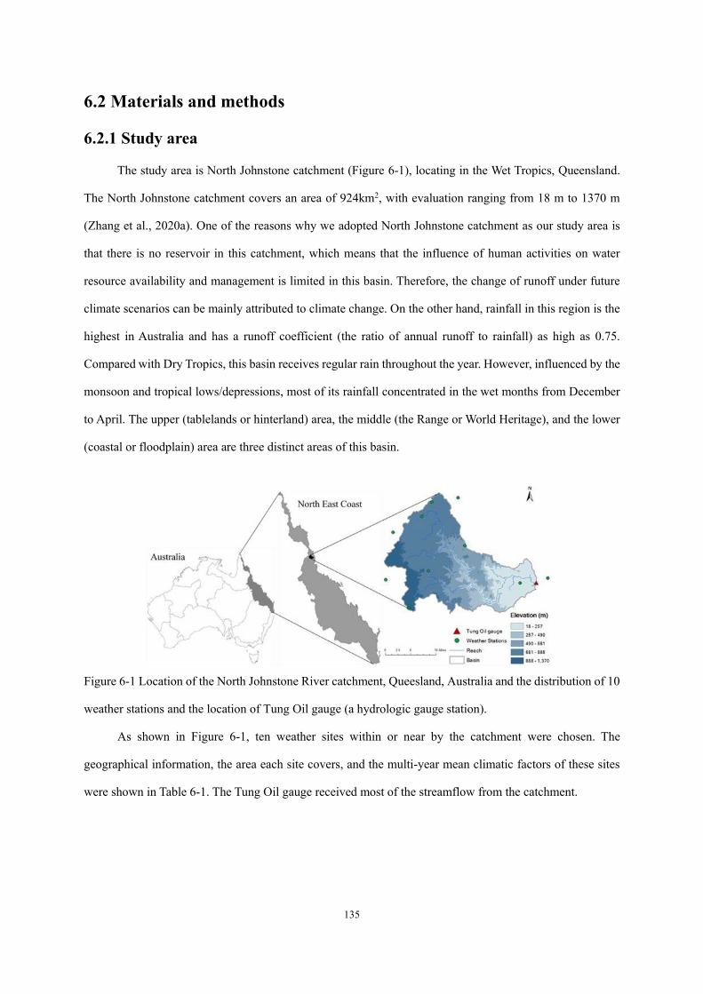
135

6.2 Materials and methods

6.2.1 Study area

The study area is North Johnstone catchment (Figure 6-1), locating in the Wet Tropics, Queensland.

The North Johnstone catchment covers an area of 924km2, with evaluation ranging from 18 m to 1370 m

(Zhang et al., 2020a). One of the reasons why we adopted North Johnstone catchment as our study area is

that there is no reservoir in this catchment, which means that the influence of human activities on water

resource availability and management is limited in this basin. Therefore, the change of runoff under future

climate scenarios can be mainly attributed to climate change. On the other hand, rainfall in this region is the

highest in Australia and has a runoff coefficient (the ratio of annual runoff to rainfall) as high as 0.75.

Compared with Dry Tropics, this basin receives regular rain throughout the year. However, influenced by the

monsoon and tropical lows/depressions, most of its rainfall concentrated in the wet months from December

to April. The upper (tablelands or hinterland) area, the middle (the Range or World Heritage), and the lower

(coastal or floodplain) area are three distinct areas of this basin.

Figure 6-1 Location of the North Johnstone River catchment, Queesland, Australia and the distribution of 10

weather stations and the location of Tung Oil gauge (a hydrologic gauge station).

As shown in Figure 6-1, ten weather sites within or near by the catchment were chosen. The

geographical information, the area each site covers, and the multi-year mean climatic factors of these sites

were shown in Table 6-1. The Tung Oil gauge received most of the streamflow from the catchment.

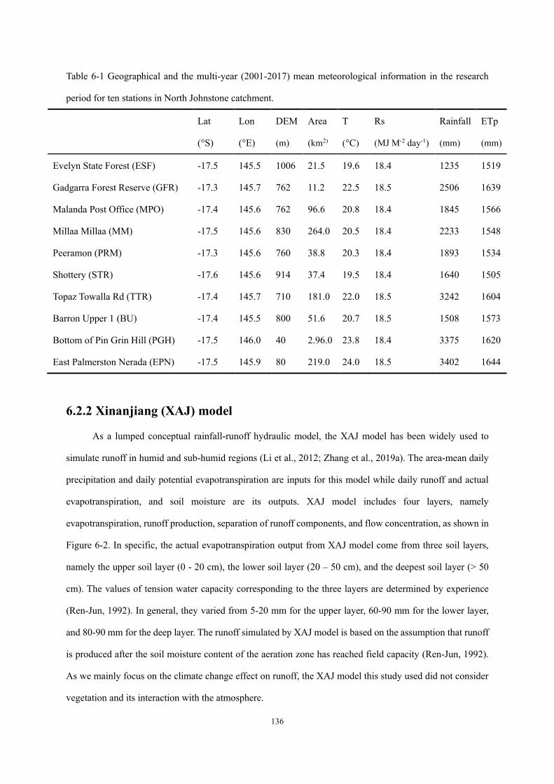
136

Table 6-1 Geographical and the multi-year (2001-2017) mean meteorological information in the research

period for ten stations in North Johnstone catchment.

Lat Lon DEM Area T Rs Rainfall ETp

(°S) (°E) (m) (km2) (°C) (MJ M-2 day-1) (mm) (mm)

Evelyn State Forest (ESF) -17.5 145.5 1006 21.5 19.6 18.4 1235 1519

Gadgarra Forest Reserve (GFR) -17.3 145.7 762 11.2 22.5 18.5 2506 1639

Malanda Post Office (MPO) -17.4 145.6 762 96.6 20.8 18.4 1845 1566

Millaa Millaa (MM) -17.5 145.6 830 264.0 20.5 18.4 2233 1548

Peeramon (PRM) -17.3 145.6 760 38.8 20.3 18.4 1893 1534

Shottery (STR) -17.6 145.6 914 37.4 19.5 18.4 1640 1505

Topaz Towalla Rd (TTR) -17.4 145.7 710 181.0 22.0 18.5 3242 1604

Barron Upper 1 (BU) -17.4 145.5 800 51.6 20.7 18.5 1508 1573

Bottom of Pin Grin Hill (PGH) -17.5 146.0 40 2.96.0 23.8 18.4 3375 1620

East Palmerston Nerada (EPN) -17.5 145.9 80 219.0 24.0 18.5 3402 1644

6.2.2 Xinanjiang (XAJ) model

As a lumped conceptual rainfall-runoff hydraulic model, the XAJ model has been widely used to

simulate runoff in humid and sub-humid regions (Li et al., 2012; Zhang et al., 2019a). The area-mean daily

precipitation and daily potential evapotranspiration are inputs for this model while daily runoff and actual

evapotranspiration, and soil moisture are its outputs. XAJ model includes four layers, namely

evapotranspiration, runoff production, separation of runoff components, and flow concentration, as shown in

Figure 6-2. In specific, the actual evapotranspiration output from XAJ model come from three soil layers,

namely the upper soil layer (0 - 20 cm), the lower soil layer (20 – 50 cm), and the deepest soil layer (> 50

cm). The values of tension water capacity corresponding to the three layers are determined by experience

(Ren-Jun, 1992). In general, they varied from 5-20 mm for the upper layer, 60-90 mm for the lower layer,

and 80-90 mm for the deep layer. The runoff simulated by XAJ model is based on the assumption that runoff

is produced after the soil moisture content of the aeration zone has reached field capacity (Ren-Jun, 1992).

As we mainly focus on the climate change effect on runoff, the XAJ model this study used did not consider

vegetation and its interaction with the atmosphere.

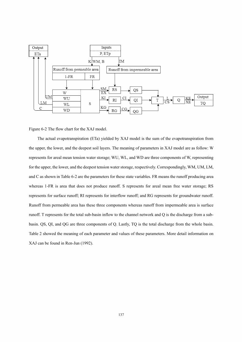
137

Figure 6-2 The flow chart for the XAJ model.

The actual evapotranspiration (ETa) yielded by XAJ model is the sum of the evapotranspiration from

the upper, the lower, and the deepest soil layers. The meaning of parameters in XAJ model are as follow: W

represents for areal mean tension water storage; WU, WL, and WD are three components of W, representing

for the upper, the lower, and the deepest tension water storage, respectively. Correspondingly, WM, UM, LM,

and C as shown in Table 6-2 are the parameters for these state variables. FR means the runoff producing area

whereas 1-FR is area that does not produce runoff. S represents for areal mean free water storage; RS

represents for surface runoff; RI represents for interflow runoff; and RG represents for groundwater runoff.

Runoff from permeable area has these three components whereas runoff from impermeable area is surface

runoff. T represents for the total sub-basin inflow to the channel network and Q is the discharge from a sub-

basin. QS, QI, and QG are three components of Q. Lastly, TQ is the total discharge from the whole basin.

Table 2 showed the meaning of each parameter and values of these parameters. More detail information on

XAJ can be found in Ren-Jun (1992).

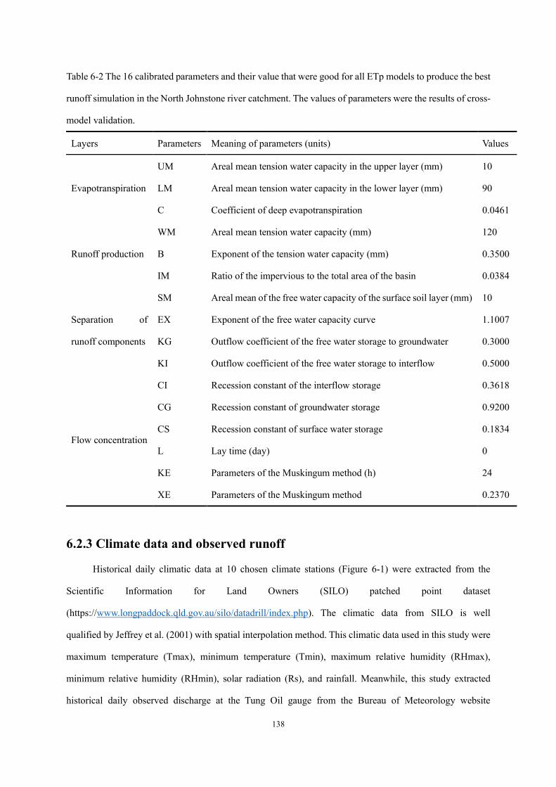
138

Table 6-2 The 16 calibrated parameters and their value that were good for all ETp models to produce the best

runoff simulation in the North Johnstone river catchment. The values of parameters were the results of cross-

model validation.

Layers Parameters Meaning of parameters (units) Values

Evapotranspiration

UM Areal mean tension water capacity in the upper layer (mm) 10

LM Areal mean tension water capacity in the lower layer (mm) 90

C Coefficient of deep evapotranspiration 0.0461

Runoff production

WM Areal mean tension water capacity (mm) 120

B Exponent of the tension water capacity (mm) 0.3500

IM Ratio of the impervious to the total area of the basin 0.0384

Separation of

runoff components

SM Areal mean of the free water capacity of the surface soil layer (mm) 10

EX Exponent of the free water capacity curve 1.1007

KG Outflow coefficient of the free water storage to groundwater 0.3000

KI Outflow coefficient of the free water storage to interflow 0.5000

Flow concentration

CI Recession constant of the interflow storage 0.3618

CG Recession constant of groundwater storage 0.9200

CS Recession constant of surface water storage 0.1834

L Lay time (day) 0

KE Parameters of the Muskingum method (h) 24

XE Parameters of the Muskingum method 0.2370

6.2.3 Climate data and observed runoff

Historical daily climatic data at 10 chosen climate stations (Figure 6-1) were extracted from the

Scientific Information for Land Owners (SILO) patched point dataset

(https://www.longpaddock.qld.gov.au/silo/datadrill/index.php). The climatic data from SILO is well

qualified by Jeffrey et al. (2001) with spatial interpolation method. This climatic data used in this study were

maximum temperature (Tmax), minimum temperature (Tmin), maximum relative humidity (RHmax),

minimum relative humidity (RHmin), solar radiation (Rs), and rainfall. Meanwhile, this study extracted

historical daily observed discharge at the Tung Oil gauge from the Bureau of Meteorology website

139

(http://www.bom.gov.au/waterdata/) to calibrate and validate XAJ model.

In addition to historical climate data, daily climatic data including Tmax, Tmin, Rs, and rainfall under

RCP4.5 and RCP8.5 scenarios were downscaled from 34 global climate models (GCMs). The downscale

method was developed by Liu and Zuo (2012) and has been widely used in the assessment of climate change

effects on drought (Feng et al., 2018a), crop yield (Ruan et al., 2018), rainfall (Feng et al., 2018b), and runoff

projection (Zhang et al., 2019a).

6.2.4 The remote sensing-based evapotranspiration product and empirical

ETp models

The PML-V1 and PML-V2 are two different versions of Penman-Monteith-Leuning model, which

accounts for the physical features of canopy and soil water loss to more accurately estimate surface

conductance (Leuning et al., 2008). Compared with PML-V1, which couples Leuning surface conductance

model with Penman-Monteith model to estimate transpiration from the plant canopy (Zhang et al., 2016), the

PML-V2 model uses a water-carbon coupled canopy conductance model to estimate ET based on remote

sensed leaf area index, albedo, and surface emissivity (Gan et al., 2018). Lately, Zhang et al. (2019b) furtherly

improved PML-V2 model by incorporating the vapor pressure deficit to constrain canopy conductance and

transpiration. Thus, PML-V2 can assess the influence of change in CO2 concentration on canopy conductance

and plant evapotranspiration. The resolution of global PML-V2 is 500 m and 8-day. It is generated by using

500-m Moderate Resolution Imaging Spectroradiometer (MODIS) remote sensing data in the Google Earth

Engine. In Zhang et al. (2019b), they compared and validated the 8-day evapotranspiration product with the

8-day evapotranspiration measurements by 95 widely-distributed flux towers from 2002 to 2017. They found

that the RMSE and bias between the PML_V2 ET and measured ET was 0.69 mm day-1 and -1.8%. The

RMSE and bias during the leave-one-out cross-validation was 0.73 mm day-1 and -3%. They concluded that

the PML_V2 products are significantly better than most global evapotranspiration products. Thus, in this

study we included evapotranspiration extracted from this product as the benchmark. The global PML-V2

products are freely accessed for global water and carbon studies through the Google Earth Engine and more

details about this product can be found in Zhang et al. (2019b). The PML-V2 products have been updated to

May 2020 from February 2000. Zhang et al. (2020b) simulated runoff at ungauged regions across Australia

with PML_V2 to drive XAJ and SIMHYD models and found that PML_V2 was reliable in simulating montly

runoff and mean annual runoff.

140

In addition to PML_V2, empirical models including the physically-based Penman model, radiation-

based Jensen-Haise (JH), Abtew (Ab), and modified Makkink (Mak), and temperature-based Hargreaves (HS)

models were also used to drive XAJ model. ETp estimated by these models was firstly accumulated into 8-

day ETp, then input the 8-day ETp into XAJ model to simulate runoff. Thus, to evaluate the difference of

XAJ model in simulating runoff with empirical ETp models and PML_V2.

6.2.5 Calibration and validation of XAJ model

The historical climatic data and observed runoff data from 2000 to 2010 were used to calibrate XAJ

model while the data from 2011 to 2017 were used for model’s validation. This study used SCE-UA (Shuffled

Complex Evolution method developed at the University of Arizona), a global optimization method to

optimize XAJ model parameters. As different ETp models were used to calculate ETp and drive XAJ model,

the parameters calibrated by a certain ETp model were also used to validate XAJ model for other ETp models

in addition to the one used for calibration. In other words, cross-model validation was carried out among

these ETp models to investigate the sensitivity of XAJ model to different ETp models. The parameters that

produced for the best runoff simulation for all ETp models were then used in runoff projection with

downscaled climatic data under future climate scenarios, as shown in Table 6-2. To project the change of

runoff in the future period, we divided the downscaled climatic data into five time periods, namely baseline

period from 2001 to 2020; near future period from 2021 to 2040 (2030s); middle future period from 2041 to

2060 (2050s); far future period from 2061 to 2080 (2070s); and further future period from 2081 to 2100

(2090s).

6.2.6 Evaluation of model performance

Nash-Sutcliffe Efficiency (NSE), coefficient of determination (R2), and root mean square error (RMSE)

were used to evaluate the performance of the XAJ model driven by different models-estimated ETp. The

NSE has been widely used in comparing hydrologic model performance (Fang et al., 2020; Li et al., 2009).

It ranges from -∞ to 1. The value of 1 represents that the model-simulated runoff perfectly matches with the

observed runoff. Therefore, the closer the NSE value is to 1, the better the hydrological model performs.

Generally, a hydrological model with NSE and R2 larger than 0.50 is capable to effectively simulate stream

flow for a certain catchment (Zhang et al., 2019a). The NSE, R2, and MBE were calculated with the following

equations:

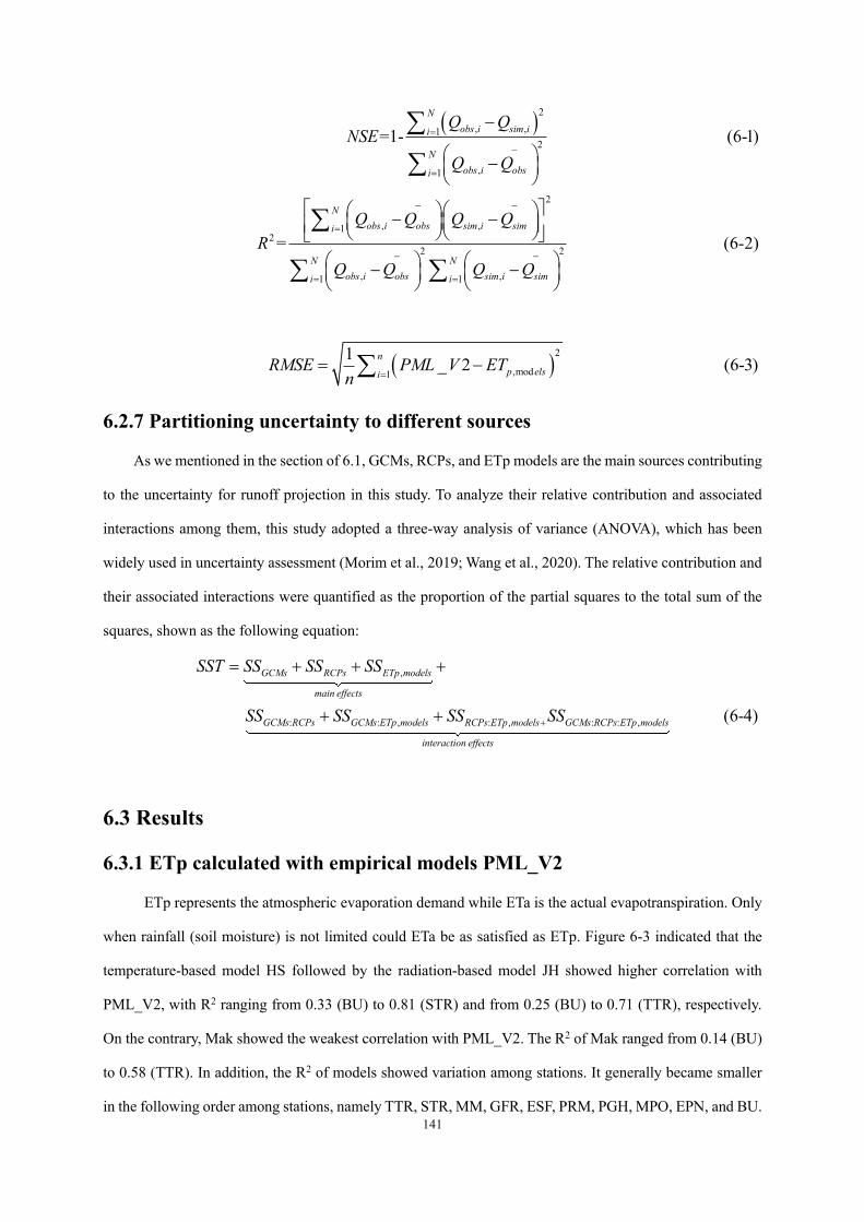
141

( )2

, ,12

,1

=1- (6-1)N

obs i sim ii

Nobs i obsi

Q QNSE

Q Q

=

−

=

−

−

( )2

,mod1

1 _ 2 (6-3)np elsi

RMSE PML V ETn =

= −

6.2.7 Partitioning uncertainty to different sources

As we mentioned in the section of 6.1, GCMs, RCPs, and ETp models are the main sources contributing

to the uncertainty for runoff projection in this study. To analyze their relative contribution and associated

interactions among them, this study adopted a three-way analysis of variance (ANOVA), which has been

widely used in uncertainty assessment (Morim et al., 2019; Wang et al., 2020). The relative contribution and

their associated interactions were quantified as the proportion of the partial squares to the total sum of the

squares, shown as the following equation:

,

: : , : , : : , (6-4)

GCMs RCPs ETp models

main effects

GCMs RCPs GCMs ETp models RCPs ETp models GCMs RCPs ETp models

interaction effects

SST SS SS SS

SS SS SS SS+

= + + +

+ +

6.3 Results

6.3.1 ETp calculated with empirical models PML_V2

ETp represents the atmospheric evaporation demand while ETa is the actual evapotranspiration. Only

when rainfall (soil moisture) is not limited could ETa be as satisfied as ETp. Figure 6-3 indicated that the

temperature-based model HS followed by the radiation-based model JH showed higher correlation with

PML_V2, with R2 ranging from 0.33 (BU) to 0.81 (STR) and from 0.25 (BU) to 0.71 (TTR), respectively.

On the contrary, Mak showed the weakest correlation with PML_V2. The R2 of Mak ranged from 0.14 (BU)

to 0.58 (TTR). In addition, the R2 of models showed variation among stations. It generally became smaller

in the following order among stations, namely TTR, STR, MM, GFR, ESF, PRM, PGH, MPO, EPN, and BU.

2

, ,12

2 2

, ,1 1

= (6-2)

Nobs i obs sim i simi

N Nobs i obs sim i simi i

Q Q Q QR

Q Q Q Q

− −

=

− −

= =

− −

− −

142

In terms of RMSE, Ab and HS generally produced smaller values than other models. For instance, RMSE

produced by HS ranged from 0.70 mm day-1 to 1.42 mm day-1 whereas JH model, despite the high R2

produced higher RMSE, ranging from 1.23 mm day-1 to 2.59 mm day-1. In summary, model HS showed both

higher R2 and lower RMSE, thus was the model that produce the closest ET estimation as PML_V2 did.

Figure 6-3 Scatter plots of the daily ETa (mm day-1) estimated by PML_V2 vs ETp estimated by empirical

ETp models from 2000 to 2017 for each of ten stations in North Johnstone river catchment, Queensland,

Australia. The unit for RMSE is mm day-1. The red and the blue lines represent the 1:1 lines and the linear

regression lines, respectively.

6.3.2 XAJ model calibration and cross-model validation

Calibrated parameters with the chosen ETp models for XAJ model in the North Johnstone river

catchment were shown in Table 6-3. With the six group of parameters, the performance of XAJ model driven

by different ETp models were assessed via the statistical indexes (R2, NSE, RMSE) between the observed

and the simulated runoff, as shown in Table 6-4.

RMSE=1.03 R2=0.57

RMSE=1.28 R2=0.70

RMSE=1.87 R2=0.61

RMSE=1.32 R2=0.49

RMSE=1.74 R2=0.57

RMSE=0.82 R2=0.59

RMSE=0.82 R2=0.78

RMSE=1.73 R2=0.63

RMSE=0.89 R2=0.51

RMSE=1.33 R2=0.62

RMSE=0.94 R2=0.47

RMSE=0.96 R2=0.63

RMSE=1.58 R2=0.54

RMSE=1.05 R2=0.39

RMSE=1.38 R2=0.48

RMSE=0.78 R2=0.60

RMSE=0.70 R2=0.78

RMSE=1.31 R2=0.65

RMSE=0.90 R2=0.51

RMSE=1.12 R2=0.62

RMSE=0.90 R2=0.50

RMSE=0.75 R2=0.66

RMSE=1.23 R2=0.56

RMSE=0.94 R2=0.42

RMSE=1.09 R2=0.52

RMSE=0.69 R2=0.66

RMSE=0.77 R2=0.81

RMSE=1.39 R2=0.67

RMSE=0.91 R2=0.56

RMSE=1.23 R2=0.66

RMSE=1.09 R2=0.67

RMSE=1.26 R2=0.80

RMSE=2.10 R2=0.71

RMSE=1.22 R2=0.58

RMSE=1.72 R2=0.68

RMSE=1.34 R2=0.19

RMSE=1.37 R2=0.33

RMSE=1.90 R2=0.25

RMSE=1.41 R2=0.14

RMSE=1.76 R2=0.19

RMSE=0.94 R2=0.50

RMSE=0.78 R2=0.67

RMSE=1.80 R2=0.55

RMSE=0.98 R2=0.42

RMSE=1.24 R2=0.52

RMSE=1.46 R2=0.38

RMSE=1.42 R2=0.51

RMSE=2.59 R2=0.42

RMSE=1.43 R2=0.30

RMSE=1.96 R2=0.38

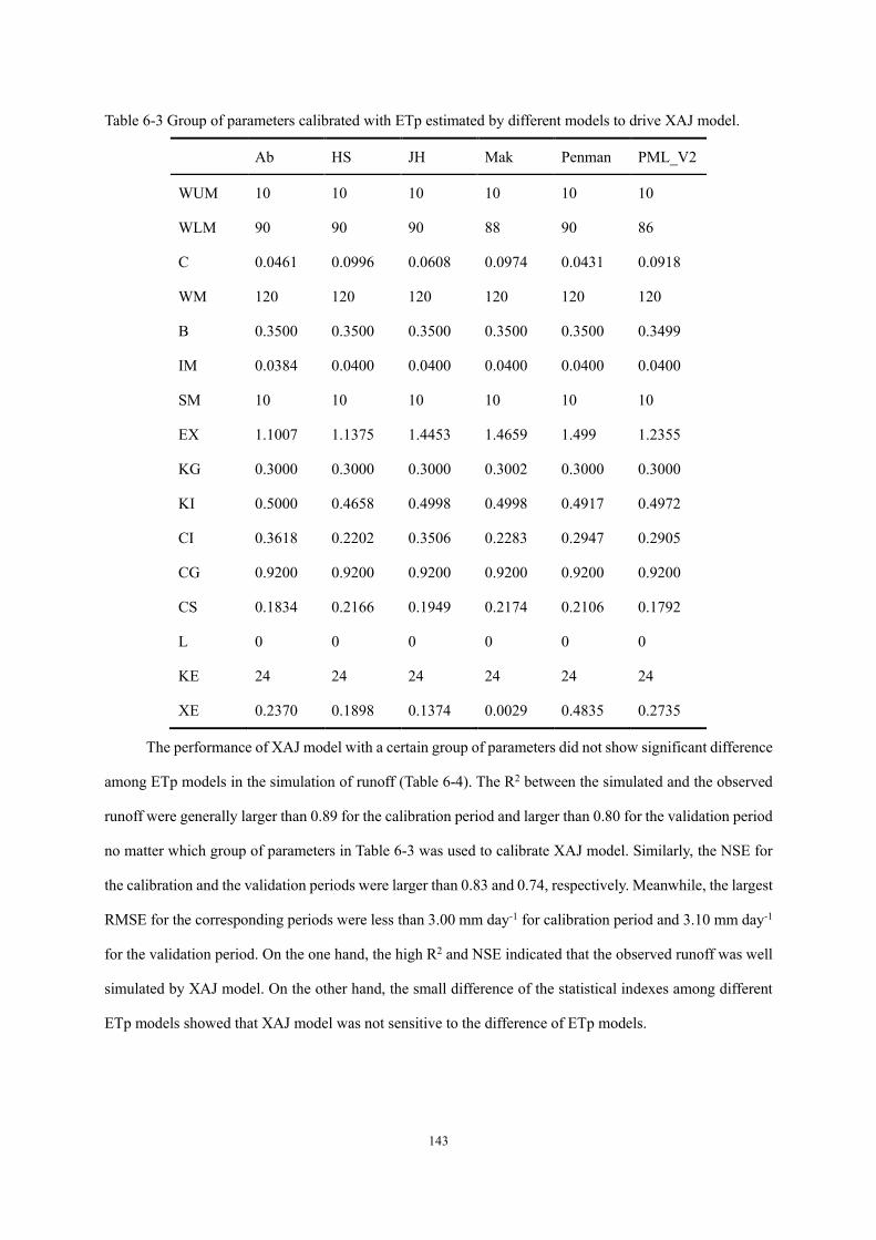
143

Table 6-3 Group of parameters calibrated with ETp estimated by different models to drive XAJ model.

Ab HS JH Mak Penman PML_V2

WUM 10 10 10 10 10 10

WLM 90 90 90 88 90 86

C 0.0461 0.0996 0.0608 0.0974 0.0431 0.0918

WM 120 120 120 120 120 120

B 0.3500 0.3500 0.3500 0.3500 0.3500 0.3499

IM 0.0384 0.0400 0.0400 0.0400 0.0400 0.0400

SM 10 10 10 10 10 10

EX 1.1007 1.1375 1.4453 1.4659 1.499 1.2355

KG 0.3000 0.3000 0.3000 0.3002 0.3000 0.3000

KI 0.5000 0.4658 0.4998 0.4998 0.4917 0.4972

CI 0.3618 0.2202 0.3506 0.2283 0.2947 0.2905

CG 0.9200 0.9200 0.9200 0.9200 0.9200 0.9200

CS 0.1834 0.2166 0.1949 0.2174 0.2106 0.1792

L 0 0 0 0 0 0

KE 24 24 24 24 24 24

XE 0.2370 0.1898 0.1374 0.0029 0.4835 0.2735

The performance of XAJ model with a certain group of parameters did not show significant difference

among ETp models in the simulation of runoff (Table 6-4). The R2 between the simulated and the observed

runoff were generally larger than 0.89 for the calibration period and larger than 0.80 for the validation period

no matter which group of parameters in Table 6-3 was used to calibrate XAJ model. Similarly, the NSE for

the calibration and the validation periods were larger than 0.83 and 0.74, respectively. Meanwhile, the largest

RMSE for the corresponding periods were less than 3.00 mm day-1 for calibration period and 3.10 mm day-1

for the validation period. On the one hand, the high R2 and NSE indicated that the observed runoff was well

simulated by XAJ model. On the other hand, the small difference of the statistical indexes among different

ETp models showed that XAJ model was not sensitive to the difference of ETp models.

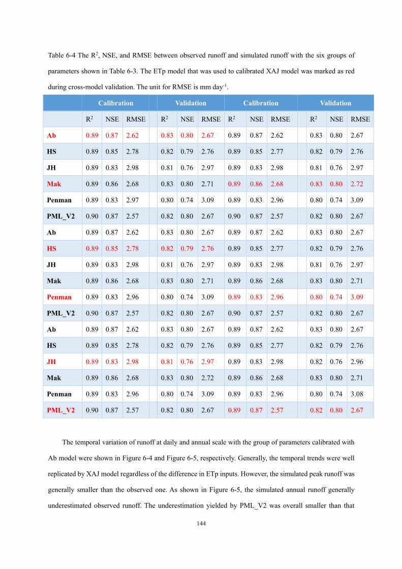
144

Table 6-4 The R2, NSE, and RMSE between observed runoff and simulated runoff with the six groups of

parameters shown in Table 6-3. The ETp model that was used to calibrated XAJ model was marked as red

during cross-model validation. The unit for RMSE is mm day-1.

Calibration Validation Calibration Validation

R2 NSE RMSE R2 NSE RMSE R2 NSE RMSE R2 NSE RMSE

Ab 0.89 0.87 2.62 0.83 0.80 2.67 0.89 0.87 2.62 0.83 0.80 2.67

HS 0.89 0.85 2.78 0.82 0.79 2.76 0.89 0.85 2.77 0.82 0.79 2.76

JH 0.89 0.83 2.98 0.81 0.76 2.97 0.89 0.83 2.98 0.81 0.76 2.97

Mak 0.89 0.86 2.68 0.83 0.80 2.71 0.89 0.86 2.68 0.83 0.80 2.72

Penman 0.89 0.83 2.97 0.80 0.74 3.09 0.89 0.83 2.96 0.80 0.74 3.09

PML_V2 0.90 0.87 2.57 0.82 0.80 2.67 0.90 0.87 2.57 0.82 0.80 2.67

Ab 0.89 0.87 2.62 0.83 0.80 2.67 0.89 0.87 2.62 0.83 0.80 2.67

HS 0.89 0.85 2.78 0.82 0.79 2.76 0.89 0.85 2.77 0.82 0.79 2.76

JH 0.89 0.83 2.98 0.81 0.76 2.97 0.89 0.83 2.98 0.81 0.76 2.97

Mak 0.89 0.86 2.68 0.83 0.80 2.71 0.89 0.86 2.68 0.83 0.80 2.71

Penman 0.89 0.83 2.96 0.80 0.74 3.09 0.89 0.83 2.96 0.80 0.74 3.09

PML_V2 0.90 0.87 2.57 0.82 0.80 2.67 0.90 0.87 2.57 0.82 0.80 2.67

Ab 0.89 0.87 2.62 0.83 0.80 2.67 0.89 0.87 2.62 0.83 0.80 2.67

HS 0.89 0.85 2.78 0.82 0.79 2.76 0.89 0.85 2.77 0.82 0.79 2.76

JH 0.89 0.83 2.98 0.81 0.76 2.97 0.89 0.83 2.98 0.82 0.76 2.96

Mak 0.89 0.86 2.68 0.83 0.80 2.72 0.89 0.86 2.68 0.83 0.80 2.71

Penman 0.89 0.83 2.96 0.80 0.74 3.09 0.89 0.83 2.96 0.80 0.74 3.08

PML_V2 0.90 0.87 2.57 0.82 0.80 2.67 0.89 0.87 2.57 0.82 0.80 2.67

The temporal variation of runoff at daily and annual scale with the group of parameters calibrated with

Ab model were shown in Figure 6-4 and Figure 6-5, respectively. Generally, the temporal trends were well

replicated by XAJ model regardless of the difference in ETp inputs. However, the simulated peak runoff was

generally smaller than the observed one. As shown in Figure 6-5, the simulated annual runoff generally

underestimated observed runoff. The underestimation yielded by PML_V2 was overall smaller than that

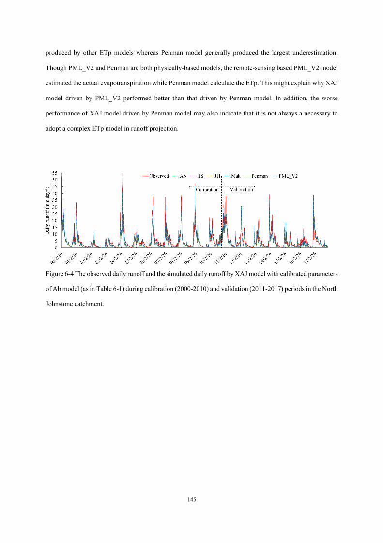
145

produced by other ETp models whereas Penman model generally produced the largest underestimation.

Though PML_V2 and Penman are both physically-based models, the remote-sensing based PML_V2 model

estimated the actual evapotranspiration while Penman model calculate the ETp. This might explain why XAJ

model driven by PML_V2 performed better than that driven by Penman model. In addition, the worse

performance of XAJ model driven by Penman model may also indicate that it is not always a necessary to

adopt a complex ETp model in runoff projection.

Figure 6-4 The observed daily runoff and the simulated daily runoff by XAJ model with calibrated parameters

of Ab model (as in Table 6-1) during calibration (2000-2010) and validation (2011-2017) periods in the North

Johnstone catchment.

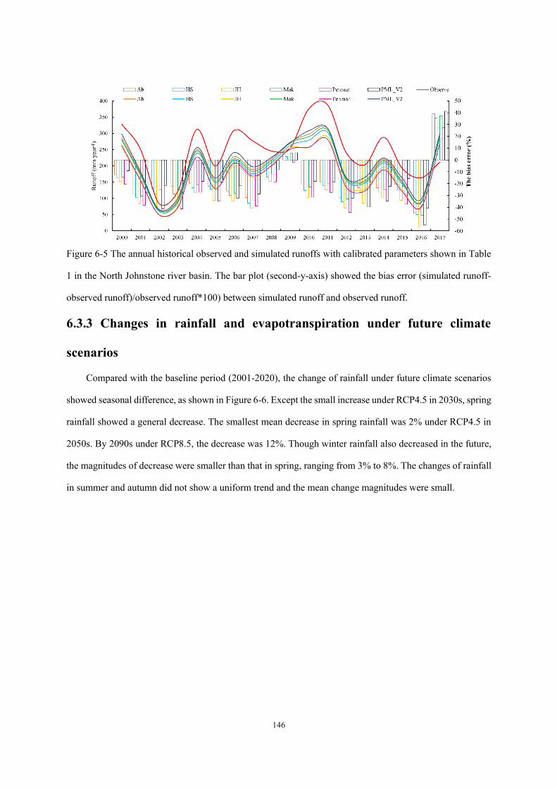
146

Figure 6-5 The annual historical observed and simulated runoffs with calibrated parameters shown in Table

1 in the North Johnstone river basin. The bar plot (second-y-axis) showed the bias error (simulated runoff-

observed runoff)/observed runoff*100) between simulated runoff and observed runoff.

6.3.3 Changes in rainfall and evapotranspiration under future climate

scenarios

Compared with the baseline period (2001-2020), the change of rainfall under future climate scenarios

showed seasonal difference, as shown in Figure 6-6. Except the small increase under RCP4.5 in 2030s, spring

rainfall showed a general decrease. The smallest mean decrease in spring rainfall was 2% under RCP4.5 in

2050s. By 2090s under RCP8.5, the decrease was 12%. Though winter rainfall also decreased in the future,

the magnitudes of decrease were smaller than that in spring, ranging from 3% to 8%. The changes of rainfall

in summer and autumn did not show a uniform trend and the mean change magnitudes were small.

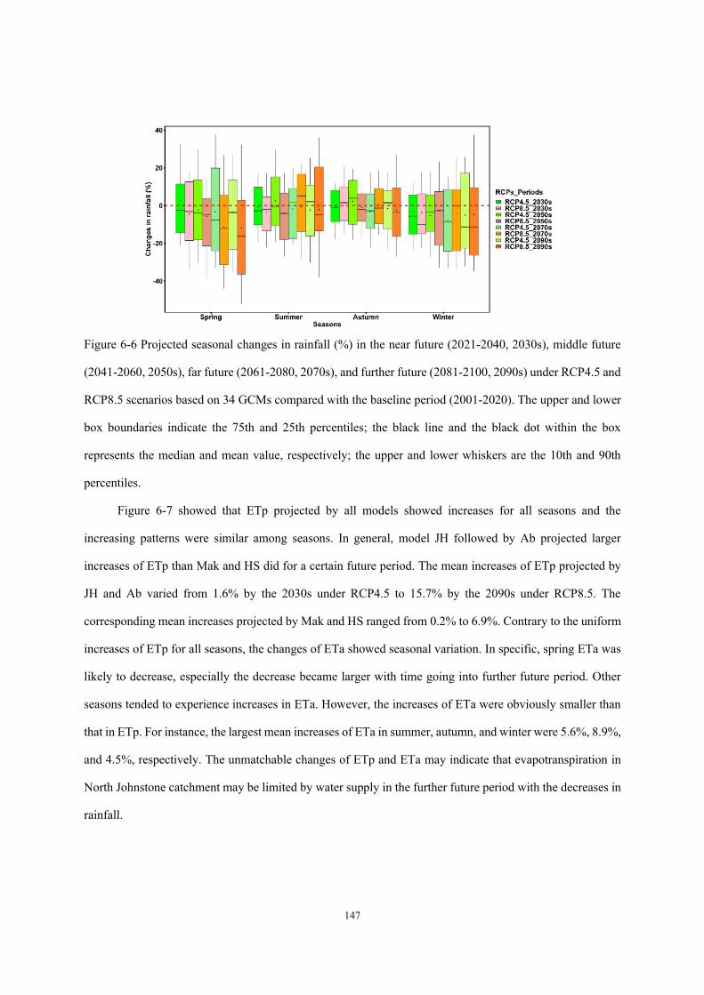
147

Figure 6-6 Projected seasonal changes in rainfall (%) in the near future (2021-2040, 2030s), middle future

(2041-2060, 2050s), far future (2061-2080, 2070s), and further future (2081-2100, 2090s) under RCP4.5 and

RCP8.5 scenarios based on 34 GCMs compared with the baseline period (2001-2020). The upper and lower

box boundaries indicate the 75th and 25th percentiles; the black line and the black dot within the box

represents the median and mean value, respectively; the upper and lower whiskers are the 10th and 90th

percentiles. Figure 6-7 showed that ETp projected by all models showed increases for all seasons and the

increasing patterns were similar among seasons. In general, model JH followed by Ab projected larger

increases of ETp than Mak and HS did for a certain future period. The mean increases of ETp projected by

JH and Ab varied from 1.6% by the 2030s under RCP4.5 to 15.7% by the 2090s under RCP8.5. The

corresponding mean increases projected by Mak and HS ranged from 0.2% to 6.9%. Contrary to the uniform

increases of ETp for all seasons, the changes of ETa showed seasonal variation. In specific, spring ETa was

likely to decrease, especially the decrease became larger with time going into further future period. Other

seasons tended to experience increases in ETa. However, the increases of ETa were obviously smaller than

that in ETp. For instance, the largest mean increases of ETa in summer, autumn, and winter were 5.6%, 8.9%,

and 4.5%, respectively. The unmatchable changes of ETp and ETa may indicate that evapotranspiration in

North Johnstone catchment may be limited by water supply in the further future period with the decreases in

rainfall.

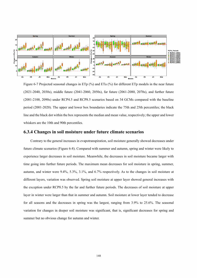
148

Figure 6-7 Projected seasonal changes in ETp (%) and ETa (%) for different ETp models in the near future

(2021-2040, 2030s), middle future (2041-2060, 2050s), far future (2061-2080, 2070s), and further future

(2081-2100, 2090s) under RCP4.5 and RCP8.5 scenarios based on 34 GCMs compared with the baseline

period (2001-2020). The upper and lower box boundaries indicate the 75th and 25th percentiles; the black

line and the black dot within the box represents the median and mean value, respectively; the upper and lower

whiskers are the 10th and 90th percentiles.

6.3.4 Changes in soil moisture under future climate scenarios

Contrary to the general increases in evapotranspiration, soil moisture generally showed decreases under

future climate scenarios (Figure 6-8). Compared with summer and autumn, spring and winter were likely to

experience larger decreases in soil moisture. Meanwhile, the decreases in soil moisture became larger with

time going into further future periods. The maximum mean decreases for soil moisture in spring, summer,

autumn, and winter were 9.4%, 5.3%, 3.1%, and 6.7% respectively. As to the changes in soil moisture at

different layers, variation was observed. Spring soil moisture at upper layer showed general increases with

the exception under RCP8.5 by the far and further future periods. The decreases of soil moisture at upper

layer in winter were larger than that in summer and autumn. Soil moisture at lower layer tended to decrease

for all seasons and the decreases in spring was the largest, ranging from 3.9% to 25.6%. The seasonal

variation for changes in deeper soil moisture was significant, that is, significant decreases for spring and

summer but no obvious change for autumn and winter.

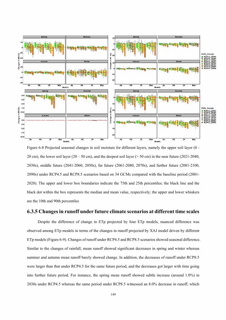
149

Figure 6-8 Projected seasonal changes in soil moisture for different layers, namely the upper soil layer (0 -

20 cm), the lower soil layer (20 – 50 cm), and the deepest soil layer (> 50 cm) in the near future (2021-2040,

2030s), middle future (2041-2060, 2050s), far future (2061-2080, 2070s), and further future (2081-2100,

2090s) under RCP4.5 and RCP8.5 scenarios based on 34 GCMs compared with the baseline period (2001-

2020). The upper and lower box boundaries indicate the 75th and 25th percentiles; the black line and the

black dot within the box represents the median and mean value, respectively; the upper and lower whiskers

are the 10th and 90th percentiles

6.3.5 Changes in runoff under future climate scenarios at different time scales

Despite the difference of change in ETp projected by four ETp models, nuanced difference was

observed among ETp models in terms of the changes in runoff projected by XAJ model driven by different

ETp models (Figure 6-9). Changes of runoff under RCP4.5 and RCP8.5 scenarios showed seasonal difference.

Similar to the changes of rainfall, mean runoff showed significant decreases in spring and winter whereas

summer and autumn mean runoff barely showed change. In addition, the decreases of runoff under RCP8.5

were larger than that under RCP4.5 for the same future period, and the decreases got larger with time going

into further future period. For instance, the spring mean runoff showed subtle increase (around 1.0%) in

2030s under RCP4.5 whereas the same period under RCP8.5 witnessed an 8.0% decrease in runoff, which

150

was even larger than the decrease (6.7%) in 2090s under RCP4.5. By 2090s under RCP8.5 the decrease for

spring runoff was largest with maximum mean decreases ranging from 15.4% to 18.2% by 2090s. The mean

decrease of winter runoff was generally smaller than the corresponding periods of that in spring, ranging

from 2.9% to 14.8%, with the largest decrease found by 2090s under RCP8.5 ranging from 6.9%-14.8%.

Figure 6-9 Projected seasonal changes in runoff (%) for different ETp models in the near future (2021-2040,

2030s), middle future (2041-2060, 2050s), far future (2061-2080, 2070s), and further future (2081-2100,

2090s) under RCP4.5 and RCP8.5 scenarios based on 34 GCMs compared with the baseline period (2001-

2020). The upper and lower box boundaries indicate the 75th and 25th percentiles; the black line and the

black dot within the box represents the median and mean value, respectively; the upper and lower whiskers

are the 10th and 90th percentiles

To disentangle the relationships among runoff and its driving factors, this study analyzed their

correlation based on Pearson correlation coefficients, shown in Figure 6-10. In general, ETp showed negative

relationships with all other factors while the other factors are generally positively related. The coefficients

between rainfall and runoff were generally larger than 0.95, showing the strongest correlation. Following

rainfall, soil moisture at the upper (WU) and lower (WL) layers also showed strong correlation with runoff,

coefficients between them ranging from 0.64 to 0.82. On the contrary, the correlation between soil moisture

at deep layer (WD) and runoff was weak. The correlation between ETa and runoff showed seasonal variation,

that is, they showed stronger relationship in spring and winter than they did in summer and autumn. As to

ETp, its relation with runoff showed variation among ETp models, namely ETp projected by HS followed

by JH showed the weakest relation with runoff while ETp projected by Ab and Mak showed stronger one.

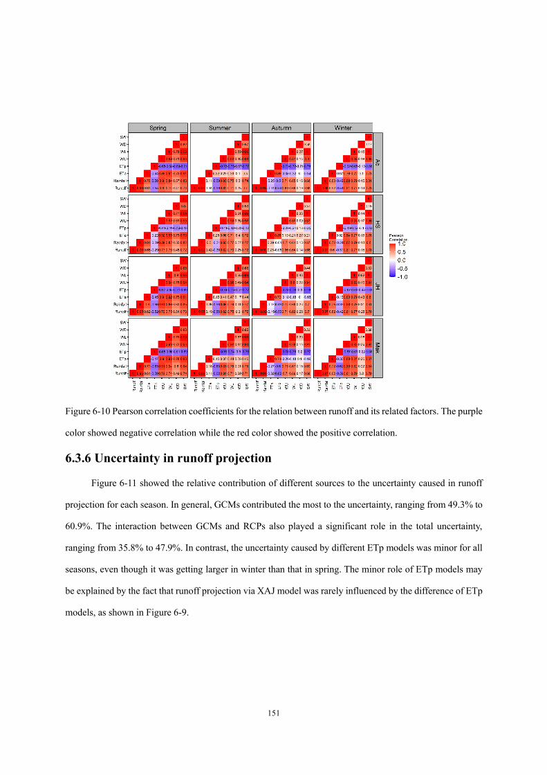
151

Figure 6-10 Pearson correlation coefficients for the relation between runoff and its related factors. The purple

color showed negative correlation while the red color showed the positive correlation.

6.3.6 Uncertainty in runoff projection

Figure 6-11 showed the relative contribution of different sources to the uncertainty caused in runoff

projection for each season. In general, GCMs contributed the most to the uncertainty, ranging from 49.3% to

60.9%. The interaction between GCMs and RCPs also played a significant role in the total uncertainty,

ranging from 35.8% to 47.9%. In contrast, the uncertainty caused by different ETp models was minor for all

seasons, even though it was getting larger in winter than that in spring. The minor role of ETp models may

be explained by the fact that runoff projection via XAJ model was rarely influenced by the difference of ETp

models, as shown in Figure 6-9.

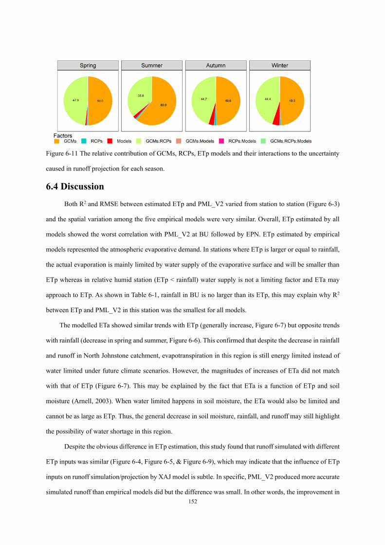
152

Figure 6-11 The relative contribution of GCMs, RCPs, ETp models and their interactions to the uncertainty

caused in runoff projection for each season.

6.4 Discussion

Both R2 and RMSE between estimated ETp and PML_V2 varied from station to station (Figure 6-3)

and the spatial variation among the five empirical models were very similar. Overall, ETp estimated by all

models showed the worst correlation with PML_V2 at BU followed by EPN. ETp estimated by empirical

models represented the atmospheric evaporative demand. In stations where ETp is larger or equal to rainfall,

the actual evaporation is mainly limited by water supply of the evaporative surface and will be smaller than

ETp whereas in relative humid station (ETp < rainfall) water supply is not a limiting factor and ETa may

approach to ETp. As shown in Table 6-1, rainfall in BU is no larger than its ETp, this may explain why R2

between ETp and PML_V2 in this station was the smallest for all models.

The modelled ETa showed similar trends with ETp (generally increase, Figure 6-7) but opposite trends

with rainfall (decrease in spring and summer, Figure 6-6). This confirmed that despite the decrease in rainfall

and runoff in North Johnstone catchment, evapotranspiration in this region is still energy limited instead of

water limited under future climate scenarios. However, the magnitudes of increases of ETa did not match

with that of ETp (Figure 6-7). This may be explained by the fact that ETa is a function of ETp and soil

moisture (Arnell, 2003). When water limited happens in soil moisture, the ETa would also be limited and

cannot be as large as ETp. Thus, the general decrease in soil moisture, rainfall, and runoff may still highlight

the possibility of water shortage in this region.

Despite the obvious difference in ETp estimation, this study found that runoff simulated with different

ETp inputs was similar (Figure 6-4, Figure 6-5, & Figure 6-9), which may indicate that the influence of ETp

inputs on runoff simulation/projection by XAJ model is subtle. In specific, PML_V2 produced more accurate

simulated runoff than empirical models did but the difference was small. In other words, the improvement in

153

runoff projection yielded by improvement of estimates in ETp was marginal (Kelleher and Shaw, 2018). This

may indicate that as a rainfall-runoff model, XAJ was not sensitive to the biases in ETp inputs. Similar to

findings in this study, Oudin et al. (2005) investigated sensitivity of four different rainfall-runoff models to

ETp inputs estimated by 27 models. They observed that temperature-based and radiation-based ETp models

was likely to provide the best runoff simulation whereas the physically-based Penman model seemed less

advantageous. In this study, the difference in changes of runoff among different ETp models under future

climate scenarios was also insignificant (Figure 6-9). In this case, it is an encouraging and convenient result

from the perspective of choice in ETp models in runoff projection in the future as climate data (e.g. wind

speed or relative humidity) from GCMs are not always available or reliable (Oudin et al., 2005; Randall et

al., 2007). However, the sensitivity of different hydrological models may be different with XAJ model, or a

drier climate may make hydrological models more sensitive to ETp inputs (Gosling and Arnell, 2011;

Kingston et al., 2009). Therefore, special attention is still needed to pay to the choice of ETp models to drive

hydrological models.

This study projected a general decrease in runoff under future climate scenarios, especially for the spring

and winter runoff (Figure 6-9). A drier future is consistent with that reported by other studies (Chiew et al.,

2010; Islam et al., 2014). For instance, Chiew et al. (2009) adopted SIMHYD, a conceptual rainfall-runoff

model, driven by climate data from 15 GCMs to project runoff across southeast Australia. They claimed that

there would be less runoff in southeast Australia under a 0.9 °C increase in surface air temperature. The

change patterns in runoff were very similar with that in rainfall (Arnell, 2003). In our study, the Pearson

correlation between runoff and rainfall was largest (Figure 6-10). This indicated that rainfall is the main

driving factors in the change of runoff. Followed rainfall, changes in soil moisture played a secondary role

in the changes of runoff. This finding was also supported by Wasko et al. (2021). The role of

evapotranspiration in runoff change is reported as that it would cause an additional reduction in runoff under

a warming climate but would not change the relative results (Charles et al., 2020). In southwest Western

Australia, Barria et al. (2015) found that runoff by 2050-2080 would decrease by 10%-80% compared to

runoff in 1970-2000 and they claimed that the reduction in runoff was mainly due to reduction in precipitation

and was strengthen by the increase in temperature. Based on Budyko’s curve, Donohue et al. (2011) assessed

the sensitivity of runoff to changes in precipitation and potential evapotranspiration. They found that despite

the spatial variation of the sensitivity of runoff showed to these two factors, the change of precipitation caused

larger change in runoff than the same change of ETp caused. The low sensitivity of runoff to ETp may also

154

partially explain why runoff projected by hydrological models driven by different ETp models did not show

much difference.

GCMs followed by interaction between GCMs and RCPs was the dominant source resulting in

uncertainty in runoff projection (Figure 6-11) (Barria et al., 2015). Similar to our study, Her et al. (2019) also

reported that the uncertainty caused by GCM projections was dominant in runoff projection. At global scale,

Arnell and Gosling (2013) also reported that uncertainty in hydrological projection was mainly dominated

by spatial difference of climate change projected by different GCMs. This may be explained by the fact that

the projection of runoff is more influenced by the projection of rainfall, which showed great uncertainty

among different GCMs (Charles et al., 2020; Rajulapati et al., 2020). The uncertainty in runoff projection

proposed challenge for decision makers in taking measures to adapt to the possible water scarcity and stress.

The possibilities to narrow uncertainty in future projection has been discussed among researchers (Hawkins

and Sutton, 2011). This study adopted the CMIP5 climatic data, with new improved modelling (CMIP6) there

is potential to reduce the uncertainty.

6.5 Conclusion

This study aimed to investigate the influence of different ETp inputs into Xinanjiang model on runoff

simulation and projection in North Johnstone catchment. In historical period, runoff simulated with empirical

ETp models was slightly worse than that simulated with PML_V2 but still showed high correlation with

observed runoff. In the future periods, runoff projected with different ETp models showed similar changes,

decreasing in spring and winter and no significant change in summer and autumn. The subtle difference

among runoff projected with different ETp models indicated that adoption of simple empirical ETp models

in runoff projection is feasible and convenient from an operational point of view as climatic data from GCMs

are not always available or reliable. The unsensitivity of Xinanjiang model to ETp models was also supported

by the relatively small contribution of ETp models to the uncertainty in runoff projection. The runoff decrease

was mainly contributed to the decrease in rainfall. Meanwhile, the unmatched magnitudes of increasing

showed by ETa and ETp and the decrease of soil moisture indicated that North Johnstone region might shift

from energy-limited to water-limited from the perspective of evapotranspiration. Lastly, the decrease of

runoff may make the water-rich North Johnstone catchment shift to the edge of decrease in water availability.

155

6.6 Reference Allan, R.P. et al., 2020. Advances in understanding large-scale responses of the water cycle to climate

change. Annals of the New York Academy of Sciences, 1472(1): 49-75.

DOI:https://doi.org/10.1111/nyas.14337

Arnell, N.W., 2003. Effects of IPCC SRES* emissions scenarios on river runoff: a global perspective. Hydrol.

Earth Syst. Sci., 7(5): 619-641. DOI:10.5194/hess-7-619-2003

Arnell, N.W., 2011. Uncertainty in the relationship between climate forcing and hydrological response in UK

catchments. Hydrol. Earth Syst. Sci., 15(3): 897-912. DOI:10.5194/hess-15-897-2011

Arnell, N.W., Gosling, S.N., 2013. The impacts of climate change on river flow regimes at the global scale.

Journal of Hydrology, 486: 351-364. DOI:https://doi.org/10.1016/j.jhydrol.2013.02.010

Bae, D.-H., Jung, I.-W., Lettenmaier, D.P., 2011. Hydrologic uncertainties in climate change from IPCC AR4

GCM simulations of the Chungju Basin, Korea. Journal of Hydrology, 401(1): 90-105.

DOI:https://doi.org/10.1016/j.jhydrol.2011.02.012

Bai, P. et al., 2016. Assessment of the Influences of Different Potential Evapotranspiration Inputs on the

Performance of Monthly Hydrological Models under Different Climatic Conditions. Journal of

Hydrometeorology, 17(8): 2259-2274. DOI:10.1175/JHM-D-15-0202.1

Barria, P., Walsh, K.J.E., Peel, M.C., Karoly, D., 2015. Uncertainties in runoff projections in southwestern

Australian catchments using a global climate model with perturbed physics. Journal of Hydrology,

529: 184-199. DOI:10.1016/j.jhydrol.2015.07.040

Charles, S.P. et al., 2020. Impact of downscaled rainfall biases on projected runoff changes. Hydrol. Earth

Syst. Sci., 24(6): 2981-2997. DOI:10.5194/hess-24-2981-2020

Chen, Y.-R., Yu, B., 2015. Impact assessment of climatic and land-use changes on flood runoff in southeast

Queensland. Evaluation de l'impact des changements climatiques et de l'utilisation des terres sur

l'écoulement de crue dans le Sud-Est du Queensland., 60(10): 1759-1769.

DOI:10.1080/02626667.2014.945938

Chiew, F., Zheng, H., Potter, N., 2018. Rainfall-Runoff Modelling Considerations to Predict Streamflow

Characteristics in Ungauged Catchments and under Climate Change. Water, 10(10): 1319.

DOI:10.3390/w10101319

Chiew, F.H.S. et al., 2010. Comparison of runoff modelled using rainfall from different downscaling methods

for historical and future climates. Journal of Hydrology, 387(1): 10-23.

DOI:https://doi.org/10.1016/j.jhydrol.2010.03.025

Chiew, F.H.S. et al., 2009. Estimating climate change impact on runoff across southeast Australia: Method,

results, and implications of the modeling method. Water Resources Research, 45(10).

DOI:doi:10.1029/2008WR007338

Chiew, F.H.S., Whetton, P.H., McMahon, T.A., Pittock, A.B., 1995. Simulation of the impacts of climate change

on runoff and soil moisture in Australian catchments Journal of Hydrology, 167(1-4): 121-147.

DOI:https://doi-org.ezproxy.lib.uts.edu.au/10.1016/0022-1694(94)02649-V

Clifton, C.F. et al., 2018. Effects of climate change on hydrology and water resources in the Blue Mountains,

Oregon, USA. Climate Services, 10: 9-19. DOI:https://doi.org/10.1016/j.cliser.2018.03.001

Dakhlaoui, H., Seibert, J., Hakala, K., 2020. Sensitivity of discharge projections to potential

evapotranspiration estimation in Northern Tunisia. Regional Environmental Change, 20(2): 34.

DOI:10.1007/s10113-020-01615-8

Donohue, R.J., Roderick, M.L., McVicar, T.R., 2011. Assessing the differences in sensitivities of runoff to

156

changes in climatic conditions across a large basin. Journal of Hydrology, 406(3): 234-244.

DOI:https://doi.org/10.1016/j.jhydrol.2011.07.003

Fang, D. et al., 2020. Combined effects of urbanization and climate change on watershed evapotranspiration

at multiple spatial scales. Journal of Hydrology, 587: 124869.

DOI:https://doi.org/10.1016/j.jhydrol.2020.124869

Feng, P. et al., 2018a. Projected changes in drought across the wheat belt of southeastern Australia using

a downscaled climate ensemble. International Journal of Climatology, 39(2): 1041-1053.

DOI:doi:10.1002/joc.5861

Feng, P. et al., 2018b. Impacts of rainfall extremes on wheat yield in semi-arid cropping systems in eastern

Australia. Climatic Change, 147(3): 555-569. DOI:10.1007/s10584-018-2170-x

Feng, Y., Cui, N., Zhao, L., Hu, X., Gong, D., 2016. Comparison of ELM, GANN, WNN and empirical models

for estimating reference evapotranspiration in humid region of Southwest China. Journal of

Hydrology, 536: 376-383. DOI:https://doi.org/10.1016/j.jhydrol.2016.02.053

Fowler, K. et al., 2018. Simulating Runoff Under Changing Climatic Conditions: A Framework for Model

Improvement. Water Resources Research, 54(12): 9812-9832.

DOI:https://doi.org/10.1029/2018WR023989

Fowler, K. et al., 2020. Many Commonly Used Rainfall ‐ Runoff Models Lack Long, Slow Dynamics:

Implications for Runoff Projections. Water Resources Research, 56(5). DOI:10.1029/2019wr025286

Freni, G., Mannina, G., Viviani, G., 2009. Urban runoff modelling uncertainty: Comparison among Bayesian

and pseudo-Bayesian methods. Environmental Modelling & Software, 24(9): 1100-1111.

DOI:https://doi.org/10.1016/j.envsoft.2009.03.003

Gan, R. et al., 2018. Use of satellite leaf area index estimating evapotranspiration and gross assimilation for

Australian ecosystems. Ecohydrology, 11(5): e1974. DOI:10.1002/eco.1974

Gosling, S.N., Arnell, N.W., 2011. Simulating current global river runoff with a global hydrological model:

model revisions, validation, and sensitivity analysis. Hydrological Processes, 25(7): 1129-1145.

DOI:doi:10.1002/hyp.7727

Guo, D., Westra, S., Maier, H.R., 2017. Impact of evapotranspiration process representation on runoff

projections from conceptual rainfall-runoff models. Water Resources Research, 53(1): 435-454.

DOI:https://doi.org/10.1002/2016WR019627

Hawkins, E., Sutton, R., 2011. The potential to narrow uncertainty in projections of regional precipitation

change. Climate Dynamics, 37(1): 407-418. DOI:10.1007/s00382-010-0810-6

Her, Y. et al., 2019. Uncertainty in hydrological analysis of climate change: multi-parameter vs. multi-GCM

ensemble predictions. Scientific Reports, 9(1): 4974. DOI:10.1038/s41598-019-41334-7

Islam, S.A., Bari, M.A., Anwar, A.H.M.F., 2014. Hydrologic impact of climate change on Murray–Hotham

catchment of Western Australia: a projection of rainfall–runoff for future water resources planning.

Hydrol. Earth Syst. Sci., 18(9): 3591-3614. DOI:10.5194/hess-18-3591-2014

Kelleher, C.A., Shaw, S.B., 2018. Is ET often oversimplified in hydrologic models? Using long records to

elucidate unaccounted for controls on ET. Journal of Hydrology, 557: 160-172.

DOI:https://doi.org/10.1016/j.jhydrol.2017.12.018

Kingston, D.G., Todd, M.C., Taylor, R.G., Thompson, J.R., Arnell, N.W., 2009. Uncertainty in the estimation of

potential evapotranspiration under climate change. Geophysical Research Letters, 36(20).

DOI:doi:10.1029/2009GL040267

Knutti, R., Sedláč ek, J., 2012. Robustness and uncertainties in the new CMIP5 climate model projections.

Nature Climate Change, 3: 369. DOI:10.1038/nclimate1716

157

https://www.nature.com/articles/nclimate1716#supplementary-information

Kumar, K.K., Kumar, K.R., Rakhecha, P., 1987. Comparison of Penman and Thornthwaite methods of

estimating potential evapotranspiration for Indian conditions. Theoretical and applied climatology,

38(3): 140-146.

Kumar Roy, D., Barzegar, R., Quilty, J., Adamowski, J., 2020. Using ensembles of adaptive neuro-fuzzy

inference system and optimization algorithms to predict reference evapotranspiration in

subtropical climatic zones. Journal of Hydrology: 125509.

DOI:https://doi.org/10.1016/j.jhydrol.2020.125509

Leuning, R., Zhang, Y.Q., Rajaud, A., Cleugh, H., Tu, K., 2008. A simple surface conductance model to

estimate regional evaporation using MODIS leaf area index and the Penman-Monteith equation.

Water Resources Research, 44(10). DOI:10.1029/2007WR006562

Li, H., Zhang, Y., 2017. Regionalising rainfall-runoff modelling for predicting daily runoff: Comparing

gridded spatial proximity and gridded integrated similarity approaches against their lumped

counterparts. Journal of Hydrology, 550: 279-293.

DOI:https://doi.org/10.1016/j.jhydrol.2017.05.015

Li, H., Zhang, Y., Chiew, F.H.S., Xu, S., 2009. Predicting runoff in ungauged catchments by using Xinanjiang

model with MODIS leaf area index. Journal of Hydrology, 370(1): 155-162.

DOI:https://doi.org/10.1016/j.jhydrol.2009.03.003

Li, H., Zhang, Y., Vaze, J., Wang, B., 2012. Separating effects of vegetation change and climate variability

using hydrological modelling and sensitivity-based approaches. Journal of Hydrology, 420-421:

403-418. DOI:https://doi.org/10.1016/j.jhydrol.2011.12.033

Li, Z., Li, Q., Wang, J., Feng, Y., Shao, Q., 2020. Impacts of projected climate change on runoff in upper reach

of Heihe River basin using climate elasticity method and GCMs. Sci Total Environ, 716: 137072.

DOI:10.1016/j.scitotenv.2020.137072

Liu, D.L., Zuo, H., 2012. Statistical downscaling of daily climate variables for climate change impact

assessment over New South Wales, Australia. Climatic Change, 115(3-4): 629-666.

DOI:10.1007/s10584-012-0464-y

Liu, W., Li, Z., Zhu, J., Xu, C., Xu, X., 2020. Dominant factors controlling runoff coefficients in karst watersheds.

Journal of Hydrology, 590: 125486. DOI:10.1016/j.jhydrol.2020.125486

Montaldo, N., Oren, R., 2018. Changing Seasonal Rainfall Distribution With Climate Directs Contrasting

Impacts at Evapotranspiration and Water Yield in the Western Mediterranean Region. Earth's

Future, 6(6): 841-856. DOI:10.1029/2018ef000843

Morim, J. et al., 2019. Robustness and uncertainties in global multivariate wind-wave climate projections.

Nature Climate Change, 9(9): 711-718. DOI:10.1038/s41558-019-0542-5

Oudin, L. et al., 2005. Which potential evapotranspiration input for a lumped rainfall–runoff model? Journal

of Hydrology, 303(1-4): 290-306. DOI:10.1016/j.jhydrol.2004.08.026

Pechlivanidis, I.G. et al., 2016. Analysis of hydrological extremes at different hydro-climatic regimes under

present and future conditions. Climatic Change, 141(3): 467-481. DOI:10.1007/s10584-016-1723-

0

Potter, N.J. et al., 2020. Bias in dynamically downscaled rainfall characteristics for hydroclimatic projections.

Hydrol. Earth Syst. Sci., 24(6): 2963-2979. DOI:10.5194/hess-24-2963-2020

Rajulapati, C.R. et al., 2020. Assessment of extremes in global precipitation products: How reliable are they?

Journal of Hydrometeorology: 1-48. DOI:10.1175/jhm-d-20-0040.1

Randall, D.A. et al., 2007. Climate models and their evaluation, Climate change 2007: The physical science

158

basis. Contribution of Working Group I to the Fourth Assessment Report of the IPCC (FAR).

Cambridge University Press, pp. 589-662.

Ren-Jun, Z., 1992. The Xinanjiang model applied in China. Journal of Hydrology, 135(1): 371-381.

DOI:https://doi.org/10.1016/0022-1694(92)90096-E

Riegger, J., Tourian, M.J., 2014. Characterization of runoff-storage relationships by satellite gravimetry and

remote sensing. Water Resources Research, 50(4): 3444-3466. DOI:10.1002/2013wr013847

Ruan, H. et al., 2018. Future climate change projects positive impacts on sugarcane productivity in southern

China. European Journal of Agronomy, 96: 108-119. DOI:https://doi.org/10.1016/j.eja.2018.03.007

Seiller, G., Anctil, F., 2016. How do potential evapotranspiration formulas influence hydrological projections?

Hydrological Sciences Journal, 61(12): 2249-2266. DOI:10.1080/02626667.2015.1100302

Sharma, A., Wasko, C., Lettenmaier, D.P., 2018. If Precipitation Extremes Are Increasing, Why Aren't Floods?

Water Resources Research, 54(11): 8545-8551. DOI:10.1029/2018wr023749

Teng, J. et al., 2015. How does bias correction of regional climate model precipitation affect modelled runoff?

Hydrol. Earth Syst. Sci., 19(2): 711-728. DOI:10.5194/hess-19-711-2015

Vaze, J., Teng, J., 2011. Future climate and runoff projections across New South Wales, Australia: results and

practical applications. Hydrological Processes, 25(1): 18-35. DOI:10.1002/hyp.7812

Wang, B. et al., 2020. Sources of uncertainty for wheat yield projections under future climate are site-

specific. Nature Food. DOI:10.1038/s43016-020-00181-w

Wasko, C., Nathan, R., 2019. Influence of changes in rainfall and soil moisture on trends in flooding. Journal

of Hydrology, 575: 432-441. DOI:10.1016/j.jhydrol.2019.05.054

Wasko, C. et al., 2021. Understanding trends in hydrologic extremes across Australia. Journal of Hydrology,

593: 125877. DOI:https://doi.org/10.1016/j.jhydrol.2020.125877

Wasko, C., Sharma, A., Lettenmaier, D.P., 2019. Increases in temperature do not translate to increased

flooding. Nat Commun, 10(1): 5676. DOI:10.1038/s41467-019-13612-5

Woldemeskel, F., Sharma, A., 2016. Should flood regimes change in a warming climate? The role of

antecedent moisture conditions. Geophysical Research Letters, 43(14): 7556-7563.

DOI:https://doi.org/10.1002/2016GL069448

Xing, W., Wang, W., Zou, S., Deng, C., 2018. Projection of future runoff change using climate elasticity

method derived from Budyko framework in major basins across China. Global and Planetary

Change, 162: 120-135. DOI:10.1016/j.gloplacha.2018.01.006

Yan, Z. et al., 2020. Ensemble Projection of Runoff in a Large‐Scale Basin: Modeling With a Global BMA

Approach. Water Resources Research, 56(7). DOI:10.1029/2019wr026134

Yang, H., Yang, D., 2011. Derivation of climate elasticity of runoff to assess the effects of climate change on

annual runoff. Water Resources Research, 47(7). DOI:10.1029/2010wr009287

Zhang, H. et al., 2019a. Impacts of future climate change on water resource availability of eastern Australia:

A case study of the Manning River basin. Journal of Hydrology, 573: 49-59.

DOI:https://doi.org/10.1016/j.jhydrol.2019.03.067

Zhang, H. et al., 2020a. Using an improved SWAT model to simulate hydrological responses to land use

change: A case study of a catchment in tropical Australia. Journal of Hydrology, 585.

DOI:10.1016/j.jhydrol.2020.124822

Zhang, Y. et al., 2020b. Can Remotely Sensed Actual Evapotranspiration Facilitate Hydrological Prediction

in Ungauged Regions Without Runoff Calibration? Water Resources Research, 56(1):

e2019WR026236. DOI:10.1029/2019wr026236

Zhang, Y. et al., 2019b. Coupled estimation of 500 m and 8-day resolution global evapotranspiration and

159

gross primary production in 2002–2017. Remote Sensing of Environment, 222: 165-182.

DOI:10.1016/j.rse.2018.12.031

Zhang, Y. et al., 2016. Multi-decadal trends in global terrestrial evapotranspiration and its components.

Scientific Reports, 6: 19124. DOI:10.1038/srep19124

https://www.nature.com/articles/srep19124#supplementary-information

Zheng, H., Chiew, F.H.S., Charles, S., Podger, G., 2018. Future climate and runoff projections across South

Asia from CMIP5 global climate models and hydrological modelling. Journal of Hydrology:

Regional Studies, 18: 92-109. DOI:10.1016/j.ejrh.2018.06.004

160

Chapter 7. Summary and future research

7.1 Summary

Evapotranspiration is an important nexus both to hydrological cycle and climate system. This study

firstly explored the capability of simplified empirical ETp models in estimating ETp rates, detecting its

temporal trends, and capturing its periodically oscillation across different climate zones. Based on findings

of which, three random forest-based models were developed as a comparison with their corresponding

empirical models including radiation-based Jensen-Haise, Abtew, modified Makkink, temperature-based

model Hargreaves in ETp estimation and projection. Then, the response of ETp, drought, and runoff to

climate change and the uncertainty in their projection under both RCP4.5 and RCP8.5 scenarios were

investigated. The main findings and insights displayed by this thesis could be summarized as the following:

(1) Radiation-based models and the temperature-based model HS generally outperformed the other two

temperature-based models and mass transfer-based models. Meanwhile, the performance of random

forest-based models outperformed their corresponding empirical models. This finding shed a light

on model choice for situations when measured evapotranspiration was not available or when the

climatic data was not supportive for the use of physically based Penman model.

(2) Despite the difference in the magnitudes estimated by different models, ETp under both RCP4.5

and RCP8.5 scenarios were likely to increase mainly due to the increase in temperature and solar

radiation. The increases of ETp showed variation among stations, namely the more arid the station

was, the larger increase of ETp showed under future climate scenarios. This may imply that the

western areas of NSW may become drier at a speed than the eastern part of NSW. More than 2/3 of

NSW is characterized with arid or semi-arid climates. The increasing of ETp suggest that the

atmospheric evaporative demand in this region is going to be stronger. In this context, some area of

NSW may shift from sub-humid or humid climates to arid or semi-arid climates without the increase

in rainfall, thus challenging the agricultural production in this region.

Uncertainty in the projection of ETp under future climate scenarios was mainly caused by the

difference of RCPs and GCMs while the contribution of ETp models was relatively small except at

humid stations. This finding highlights the importance of adopting the ensemble method with

multiple GCMs and RCPs to yield reasonable ranges of future projection.

(3) The occurrence of drought under future climate scenarios was likely to increase, especially for

161

moderate and severe droughts. Meanwhile, spring and winter would experience more increases in

drought occurrence than summer and autumn would do. Drought is one of the most serious natural

disasters agricultural production in Australia faces. There is no doubt that more moderate and severe

droughts would bring more challenge to agricultural production, or even worse making some areas

not suitable for crop production any more without proper measures for the adaption. Especially, a

few key growth periods of winter wheat happen in spring and winter, more drought occurrence in

these two seasons may bring serious reduction in crop yield. In order to adapt to the potential

negative effects resulting from more drought, new drought-resistant varieties of crop may be a

necessary. In addition, development of drought-forecasting system will also help to offer powerful

information to guide agricultural production. From the perspective of farmers, they may shift the

sowing windows accordingly to adapt to climate change effects.

Compared with historical period, the role of ETp in drought occurrence was going to improve under

future climate scenarios. This finding confirmed the suggestion that it is necessary to use drought

indexes which not only developed based on rainfall but also include evapotranspiration for drought

projection under future climate scenarios.

(4) The influence of different ETp inputs on runoff simulation and projection by Xinanjiang model was

subtle. In other words, improve the complexity of ETp models can only result in marginal

improvement for the performance of Xinanjiang model in runoff simulation. Independence of ETp

inputs, runoff projected by Xinanjing model was likely to decrease in spring and winter while the

change of summer and autumn runoff did not show uniform pattern. The patterns of runoff changes

were similar with the changes in rainfall. The decrease in runoff is possible to yield hydrological

drought and have negative effects on the tropical ecosystem. The difference in GCMs and their

interaction with RCPs were the two dominant factors leading to uncertainty in runoff projection.

The low sensitivity of Xinanjiang model to different ETp inputs is convenient and encouraging for

ETp models choice in runoff projection under future climate scenarios given the fact that not all

climatic data from GCMs have high reliability to support the use of complex ETp models.

In summary, whether it is from the perspective of agricultural drought occurrence or from the

perspective of runoff, eastern Australia is likely to face higher water stress. Agricultural production

in eastern Australia is mainly rain-fed.

162

7.2 Limitations and future research

Though this study offered useful information on performance of widely used empirical, and random

forest models in ETp estimates, their influence on drought, and runoff projection. There are a few limitations

of this study. First, performance of these ETp models was assessed against the Penman model instead of

observed evapotranspiration, which may result in bias. With the improvement in monitoring technologies,

long time sequences of observed evapotranspiration data from eddy covariance stations or remote sensing

may be available in the future. It is necessary to tap into these state-of-the-art technologies in

evapotranspiration research. Second, the key problem in existing ETp models is that existing ETp models

ignore the vegetation response to elevated CO2, leading to a higher hydrological sensitivity to temperature.

Thus, the drought projection based on such ETp models may have slightly overestimation and bias (Keenan

et al., 2020; Milly and Dunne, 2017). Thus, in future study, it is important to consider the effects of CO2

fertilization on plant evapotranspiration so that to assess the response of drought and runoff to climate change

at a more accurately level (Fowler et al., 2019; Yang et al., 2019; Yang et al., 2020). Lastly, in addition to the

difference of GCMs, RCPs, and ETp models, the downscaling method used to downscale the coarse GCMs

climatic data from global to regional scale is another key source resulting in uncertainty in future projection

(Anandhi et al., 2011; Wilby et al., 2000). This study only adopted data downscaled with a statistical

downscaling method. In future study, it is necessary to do investigation on the influence of different

downscaling methods.

163

7.3 Reference Anandhi, A. et al., 2011. Examination of change factor methodologies for climate change impact assessment.

Water Resources Research, 47(3). DOI:doi:10.1029/2010WR009104

Fowler, M.D., Kooperman, G.J., Randerson, J.T., Pritchard, M.S., 2019. The effect of plant physiological

responses to rising CO2 on global streamflow. Nature Climate Change, 9(11): 873-879.

DOI:10.1038/s41558-019-0602-x

Keenan, T.F., Luo, X., Zhang, Y., Zhou, S., 2020. Ecosystem aridity and atmospheric CO2. Science, 368(6488):

251. DOI:10.1126/science.abb5449

Milly, P.C.D., Dunne, K.A., 2017. A Hydrologic Drying Bias in Water-Resource Impact Analyses of

Anthropogenic Climate Change. JAWRA Journal of the American Water Resources Association,

53(4): 822-838. DOI:10.1111/1752-1688.12538

Wilby, R.L. et al., 2000. Hydrological responses to dynamically and statistically downscaled climate model

output. Geophysical Research Letters, 27(8): 1199-1202. DOI:doi:10.1029/1999GL006078

Yang, Y., Roderick, M.L., Zhang, S., McVicar, T.R., Donohue, R.J., 2019. Hydrologic implications of vegetation

response to elevated CO2 in climate projections. Nature Climate Change, 9(1): 44-48.

DOI:10.1038/s41558-018-0361-0

Yang, Y. et al., 2020. Comparing Palmer Drought Severity Index drought assessments using the traditional

offline approach with direct climate model outputs. Hydrology and Earth System Sciences, 24(6):

2921-2930. DOI:10.5194/hess-24-2921-2020