Climate change impacts and greenhouse gas … change impacts and greenhouse gas mitigation effects...

*Reprinted with permission from Journal of Advances in Modeling Earth Systems, 7(3): 1326–1338 ©2015 the authors

Climate change impacts and greenhouse gas mitigation effects

on U.S. water quality*Brent Boehlert, Kenneth M. Strzepek, Steven C. Chapra, Charles Fant, Yohannes Gebretsadik, Megan Lickley, Richard Swanson,

Alyssa McCluskey, James E. Neumann and Jeremy Martinich

Reprint 2015-19

The MIT Joint Program on the Science and Policy of Global Change combines cutting-edge scientific research with independent policy analysis to provide a solid foundation for the public and private decisions needed to mitigate and adapt to unavoidable global environmental changes. Being data-driven, the Program uses extensive Earth system and economic data and models to produce quantitative analysis and predictions of the risks of climate change and the challenges of limiting human influence on the environment—essential knowledge for the international dialogue toward a global response to climate change.

To this end, the Program brings together an interdisciplinary group from two established MIT research centers: the Center for Global Change Science (CGCS) and the Center for Energy and Environmental Policy Research (CEEPR). These two centers—along with collaborators from the Marine Biology Laboratory (MBL) at Woods Hole and short- and long-term visitors—provide the united vision needed to solve global challenges.

At the heart of much of the Program’s work lies MIT’s Integrated Global System Model. Through this integrated model, the Program seeks to: discover new interactions among natural and human climate system components; objectively assess uncertainty in economic and climate projections; critically and quantitatively analyze environmental management and policy proposals; understand complex connections among the many forces that will shape our future; and improve methods to model, monitor and verify greenhouse gas emissions and climatic impacts.

This reprint is one of a series intended to communicate research results and improve public understanding of global environment and energy challenges, thereby contributing to informed debate about climate change and the economic and social implications of policy alternatives.

Ronald G. Prinn and John M. Reilly, Program Co-Directors

For more information, contact the Program office: MIT Joint Program on the Science and Policy of Global Change

Postal Address: Massachusetts Institute of Technology 77 Massachusetts Avenue, E19-411 Cambridge, MA 02139 (USA)

Location: Building E19, Room 411 400 Main Street, Cambridge

Access: Tel: (617) 253-7492 Fax: (617) 253-9845 Email: [email protected] Website: http://globalchange.mit.edu/

mailto:globalchange%40mit.edu?subject=

mailto:http://globalchange.mit.edu/?subject=

RESEARCH ARTICLE10.1002/2014MS000400

Climate change impacts and greenhouse gas mitigation effectson U.S. water qualityBrent Boehlert1,2, Kenneth M. Strzepek2, Steven C. Chapra3, Charles Fant2, Yohannes Gebretsadik2,Megan Lickley2, Richard Swanson4, Alyssa McCluskey4, James E. Neumann1, and Jeremy Martinich5

1Industrial Economics, Inc., Cambridge, Massachusetts, USA, 2Joint Program on the Science and Policy of Global Change,Massachusetts Institute of Technology, Cambridge, Massachusetts, USA, 3Department of Civil and EnvironmentalEngineering, Tufts University, Medford, Massachusetts, USA, 4Civil Engineering, University of Colorado, Boulder, Colorado,USA, 5U.S. Environmental Protection Agency, Washington, District of Columbia, USA

Abstract Climate change will have potentially significant effects on freshwater quality due to increasesin river and lake temperatures, changes in the magnitude and seasonality of river runoff, and more frequentand severe extreme events. These physical impacts will in turn have economic consequences througheffects on riparian development, river and reservoir recreation, water treatment, harmful aquatic blooms,and a range of other sectors. In this paper, we analyze the physical and economic effects of changes infreshwater quality across the contiguous U.S. in futures with and without global-scale greenhouse gas miti-gation. Using a water allocation and quality model of 2119 river basins, we estimate the impacts of variousprojected emissions outcomes on several key water quality indicators, and monetize these impacts with awater quality index approach. Under mitigation, we find that water temperatures decrease considerablyand that dissolved oxygen levels rise in response. We find that the annual economic impacts on water qual-ity of a high emissions scenario rise from $1.4 billion in 2050 to $4 billion in 2100, leading to present valuemitigation benefits, discounted at 3%, of approximately $17.5 billion over the 2015–2100 period.

1. Introduction

Climate change is likely to have far-reaching impacts on water quality in the United States due to projectedincreases in air and water temperatures, more intense precipitation and runoff, and intensified extremeevents [Georgakakos et al., 2014]. Water temperature has been increasing in many rivers [Kaushal et al.,2010] and lakes [Schneider and Hook, 2010], and the length of time that lakes and reservoirs are thermallystratified has also increased [Sahoo et al., 2012; Sahoo and Schladow, 2008]. Reduced mixing, elevated watertemperatures, and biotic consumption of dissolved oxygen may lead to deteriorated water quality in lakesand ponds across the United States [Sahoo et al., 2011]. Overall, the United States (U.S.) is likely to experi-ence widespread water quality declines in lakes and rivers due to climate change and development, withchanges in water quality parameters and micropollutant concentrations expected to negatively affect drink-ing water treatment and distribution systems [Romero-Lankao and Smith, 2014].

These physical impacts on water quality will also have potentially substantial economic impacts, since waterquality is valued for a number of recreational and commercial activities including river and lake visits, boat-ing, swimming, and fishing, among others. For example, Van Houtven et al. [2014] use a contingent valua-tion study to estimate that households in Virginia would combined pay $184 million per year (in 2010dollars) to improve lake water quality through policy changes, while Boyle et al. [1998] found that a 1 mchange in water clarity at three lakes in Maine led to total property value changes in surrounding commun-ities of $16 to $22 million. Many studies have estimated the value of water quality changes at recreationalsites, for example, Bouwes and Schneider [1979] estimated a potential loss of $85,700 per year in recreationalbenefits at Pike Lake in Wisconsin due to deteriorations in water quality.

Since unmitigated climate change is projected to have negative impacts on water quality in the U.S., conse-quently leading to negative economic effects, greenhouse gas (GHG) mitigation may avoid or reduce theseadverse impacts. In this research, we present a methodology for analyzing the physical and economiceffects of climate change on freshwater quality in the contiguous U.S. (CONUS). We use a coupled water sys-tem and water quality model of 2119 river basins to evaluate the effects of global-scale GHG mitigation

Key Points:! Linked system models are critical to

assess impacts of climate change onwater quality! Mitigation reduces water

temperatures and increases DO levelsconsiderably! Economic impacts on water quality of

mitigating climate change areconsiderable

Supporting Information:! Supporting Information S1! Supporting Information S2

Correspondence to:B. Boehlert,[email protected]

Citation:Boehlert, B., K. M. Strzepek,S. C. Chapra, C. Fant, Y. Gebretsadik,M. Lickley, R. Swanson, A. McCluskey,J. E. Neumann, and J. Martinich (2015),Climate change impacts andgreenhouse gas mitigation effects onU.S. water quality, J. Adv. Model. EarthSyst., 7, 1326–1338, doi:10.1002/2014MS000400.

Received 4 NOV 2014Accepted 9 JUL 2015Accepted article online 16 JUL 2015Published online 12 SEP 2015

VC 2015. The Authors.

This is an open access article under theterms of the Creative CommonsAttribution-NonCommercial-NoDerivsLicense, which permits use anddistribution in any medium, providedthe original work is properly cited, theuse is non-commercial and nomodifications or adaptations aremade.

BOEHLERT ET AL. CLIMATE CHANGE IMPACT ON WATER QUALITY 1326

Journal of Advances in Modeling Earth Systems

PUBLICATIONS

under a range of GHG emis-sion stabilization scenarios. Toour knowledge, such a U.S.-wide nested modeling frame-work has never previouslybeen developed at this level ofdetail to evaluate water qualityimpacts and mitigation bene-fits. The results provide a firstapproximation of the physicaland economic benefits ofglobal GHG mitigation tochanges in U.S. water quality.This analysis is part of the Cli-mate Change Impacts and RiskAnalysis (CIRA) project [seeWaldhoff et al., 2014], anongoing effort to quantify andmonetize the multisector risksof inaction on climate changeand the benefits of global GHGmitigation.

2. MethodologicalApproach

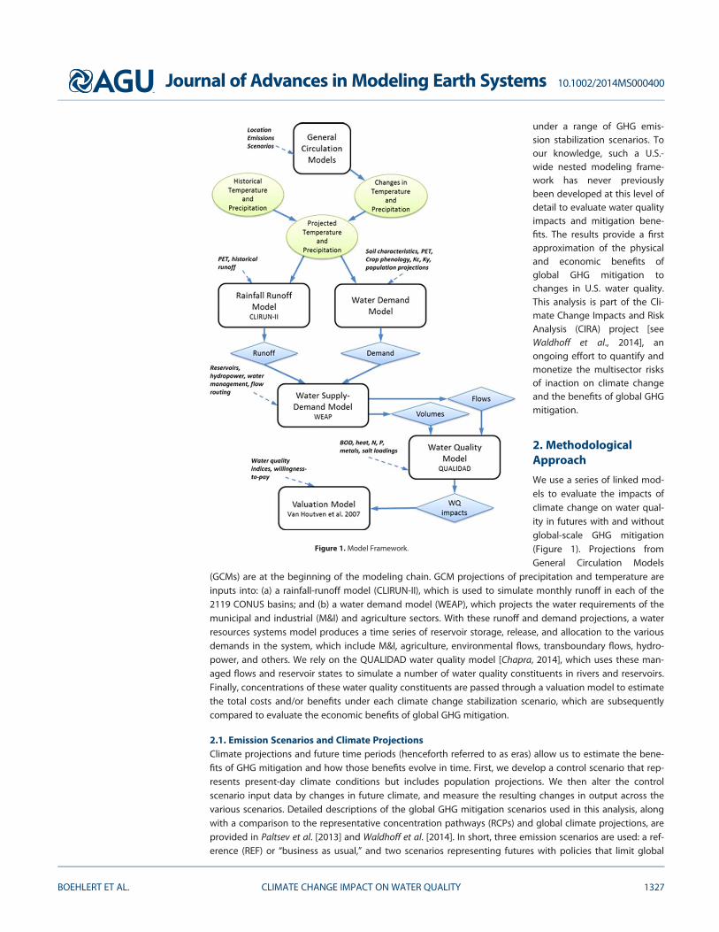
We use a series of linked mod-els to evaluate the impacts ofclimate change on water qual-ity in futures with and withoutglobal-scale GHG mitigation(Figure 1). Projections fromGeneral Circulation Models

(GCMs) are at the beginning of the modeling chain. GCM projections of precipitation and temperature areinputs into: (a) a rainfall-runoff model (CLIRUN-II), which is used to simulate monthly runoff in each of the2119 CONUS basins; and (b) a water demand model (WEAP), which projects the water requirements of themunicipal and industrial (M&I) and agriculture sectors. With these runoff and demand projections, a waterresources systems model produces a time series of reservoir storage, release, and allocation to the variousdemands in the system, which include M&I, agriculture, environmental flows, transboundary flows, hydro-power, and others. We rely on the QUALIDAD water quality model [Chapra, 2014], which uses these man-aged flows and reservoir states to simulate a number of water quality constituents in rivers and reservoirs.Finally, concentrations of these water quality constituents are passed through a valuation model to estimatethe total costs and/or benefits under each climate change stabilization scenario, which are subsequentlycompared to evaluate the economic benefits of global GHG mitigation.

2.1. Emission Scenarios and Climate ProjectionsClimate projections and future time periods (henceforth referred to as eras) allow us to estimate the bene-fits of GHG mitigation and how those benefits evolve in time. First, we develop a control scenario that rep-resents present-day climate conditions but includes population projections. We then alter the controlscenario input data by changes in future climate, and measure the resulting changes in output across thevarious scenarios. Detailed descriptions of the global GHG mitigation scenarios used in this analysis, alongwith a comparison to the representative concentration pathways (RCPs) and global climate projections, areprovided in Paltsev et al. [2013] and Waldhoff et al. [2014]. In short, three emission scenarios are used: a ref-erence (REF) or ‘‘business as usual,’’ and two scenarios representing futures with policies that limit global

Figure 1. Model Framework.

Journal of Advances in Modeling Earth Systems 10.1002/2014MS000400


GHG emissions such that total radiative forcing levels in 2100 are stabilized at 4.5 W/m2 (Policy 4.5) or 3.7W/m2 (Policy 3.7). The REF scenario has a total radiative forcing of 10.0 W/m2 in 2100. Using the IPCC simpli-fied equations, the REF has a total radiative forcing of 8.8 W/m2, and is therefore similar to representativeconcentration pathway (RCP) 8.5. The base framework used to project future climate, the CommunityAtmospheric Model linked with the MIT Integrated Global Systems Model (IGSM-CAM), is presented inMonier et al. [2013, 2014], which also provide a summary of the simulations and details on the regional pro-jections of climate change used in this study. The climate projections for each of the three GHG mitigationscenarios are split into two eras: 2050 and 2100. Each era is represented by daily climate variability (sourcedfrom Sheffield et al. [2006]) with changes in climate applied. For precipitation, we use a simple ratio methodwhere the change in precipitation is expressed as the future monthly mean precipitation divided by the his-torical monthly mean precipitation. For temperature, we use a simple ‘‘delta’’ method, where changes intemperature are expressed as differences between the mean monthly modeled historical temperature andprojected future temperature. The primary climate projections in this analysis assume a climate sensitivityof 38C; to evaluate the effect of higher climate sensitivity levels, two projections assume a sensitivity of 68C.

2.2. Runoff ModelThe climate projections for each emission scenario were used to develop monthly runoff estimates. Runoffmodeling converts the climate changes into changes in surface water availability important for the waterresource model. Surface water runoff was modeled with the rainfall-runoff model CLIRUN-II [see Strzepeket al., 2011, 2013], the latest available application in a family of hydrologic models developed specifically forthe analysis of the impact of climate change on runoff, first proposed by Kaczmarek [1993]. CLIRUN-II modelsrunoff with a lumped watershed defined by climate inputs and soil characteristics averaged over the entirewatershed, simulating runoff at a gauged location at the mouth of the catchment on a monthly time step.

CLIRUN-II has adopted a two-layer approach following the framework of the SIXPAR hydrologic model[Gupta and Sorooshian, 1983, 1985]. A unique conditional calibration procedure was used to determine thecoefficient values that characterize each of the 2119 catchments. This procedure optimizes via a patternsearch algorithm developed by MATLAB minimizing the sum of square errors of the simulated andobserved runoff. As no naturalized runoff data set for the eight-digit HUCs of CONUS is currently available,the observed runoff data used to calibrate CLIRUN-II were based on naturalized runoff data for 99 basins ofCONUS from U.S. Water Resources Council [1978]. To calibrate each eight-digit HUC, the runoff within eachof these 99 basins was allocated to the underlying eight-digit HUCs based on mean annual 1971–1980 pre-cipitation that was spatially averaged from the 1/128 3 1/128 PRISM data set [PRISM Climate Group, 2014].

Although we have confidence in the calibration runoff data set at the resolution of the 99 basins, downscal-ing these data to the 2119 eight-digit HUC introduces uncertainties. An alternative to using a calibratedrainfall-runoff model would have been to rely on a routing model such as the Variable Infiltration Capacity(VIC) or Soil Water Assessment Tool (SWAT) that are capable of simulating runoff without calibration. Theaggregated runoff outputs from these models could be validated and then ‘‘tuned’’ using the 99 basin out-flows, but no assurances exist that the runoff at the eight-digit resolution will fit naturalized observations.Efforts at the U.S. Geological Survey (USGS) are currently underway to develop an improved naturalized run-off data set for the U.S. [e.g., Farmer and Vogel, 2012], although a CONUS-wide data set is far from complete.2.2.1. Water DemandsWater demands are the other side of the water system, and are developed using 2005 data from USGS onannual water withdrawals and consumptive use in a range of sectors including irrigation, municipal, andindustrial (M&I) use, mining, thermal cooling, and several other sectors [Kenny et al., 2009]. These data areavailable at the 3109 counties of CONUS, which were spatially averaged to the eight-digit HUC resolutionusing the same approach taken by the U.S. Forest Service in their development of the Water Supply StressIndex (WaSSI) [U.S. Forest Service, 2014]. For all sectors but irrigation, we assumed that withdrawals wereconstant each day of the year, such that monthly withdrawals are apportioned from yearly values based onthe number of days in each month.

Base monthly 2005 irrigation withdrawals were developed by allocating the total annual withdrawals (fromUSGS) according to the total irrigation water requirements (IWRs) of the irrigated crop mix in each HUC.IWRs were based on the meteorological data set described above [Sheffield et al., 2006], irrigated crop areaestimates from the 2008 Farm and Ranch Irrigation Survey [U.S. Department of Agriculture, 2010], and



estimates of irrigation water depth requirements for each crop using methods developed by the U.N. Foodand Agriculture Organization (FAO) [Allen et al., 1998]. The FAO method requires estimates of potentialevapotranspiration (PET), which were calculated using the Modified Hargreaves approach [Droogers andAllen, 2002]. This procedure generated a base time series of 29 years (1980–2008) of irrigation water require-ments that vary on a monthly basis, with the 2005 annual totals summing to USGS data for each eight-digitHUC. Water requirements for each of the future eras and under each emission and climate scenario weredriven by the FAO method, which vary based on both PET and precipitation under each scenario. As aresult, total CONUS irrigation withdrawals in each era-scenario combination vary from 2005 levels.

2.3. Water Resources Planning ModelWe then simulate reservoir management and routing using a water resources systems model, where thesimulated runoff—used as surface water supply—and projected water demands are used to optimize waterallocation based on a prescribed set of priorities. This model is an adaptation of the Water Evaluation andPlanning (WEAP) model [Sieber and Purkey, 2007], a well-established river basin system modeling software.This version was rewritten in the MATLAB language for computation speed and automation, but remainsconsistent with the WEAP model methodologically, all described in detail in the WEAP documentation.

The WEAP model simulates the sequence of existing and planned reservoir activity and demand nodes alongthe system. Three demand types, or nodes, are modeled throughout the system, which are in competition forwater dependent on the sequence (upstream/downstream). The node types are municipal and industrial(M&I) water use, hydropower generation, and irrigation withdrawal. The hydrologic boundaries used to definethe basins are the 2119 eight-digit HUCs of CONUS. The structure of each basin is generic, prescribed withinput characteristics that are unique to each HUC. Reservoir data, such as locations, hydropower capabilities,and the information needed to calculate surface area and volume are all retrieved from the Army Corps ofEngineers [U.S. Army Corps of Engineers, 2013]. Hydropower production is calculated and calibrated to theNational Renewable Energy Laboratory (NREL) Regional Energy Deployment System (ReEDS) model [Shortet al., 2011]. For each of the basins, the priorities of the various water users are assumed to be in the followingorder: (1) minimum flows driven by environmental and transboundary concerns, (2) M&I water demands(including mining and thermal cooling), (3) irrigation demands, and (4) hydropower production.

2.4. Water Quality Model DescriptionUsing the managed flows from the water planning model and climate parameters, we use the QUALIDADmodel [Chapra, 2014] to track several water quality constituents for each eight-digit HUC, including temper-ature, dissolved oxygen (DO), three nitrogen species, two phosphorus species, a generic metal, and salt. Allvariables in this model have a daily time step except temperature, which is hourly. To track water qualityconstituents within the CONUS framework, each eight-digit HUC is divided into a number of segmentsbased on the Enhanced River Reach File (ERF1) from USGS [U.S. Geological Survey, 1999], which is the U.S.Environmental Protection Agency’s (EPA) digital record of over 60,000 river reaches in the U.S., intended fornational water-quality modeling. For each river segment, the data set contains corresponding parameterssuch as flow, velocity, segment length, and the sequence of segments. Based on these parameters, themain river channel is found within each eight-digit HUC, and then separated into segments at the pointswhere rivers join. The river segments are on average 16 km long, and each HUC contains approximately 30river segments, though only six or seven river segments form the main river that spans each HUC, the restare side branches feeding into the main segment. We assume that each riverbed is parabolic, following Leo-pold and Maddock [1953], which helps to derive a relationship of flow with surface area and velocity. Eachconstituent is modeled separately in each segment, and upstream to downstream mass transfer is governedusing numerical methods documented by Chapra [2007] and Chapra and Canale [2006].

QUALIDAD is a parsimonious water quality model that is designed to model daily water quality dynamics atthe basin scale. The state variables governing the DO, nitrogen, and phosphorus dynamics within the modelare shown in Table 1. A general mass balance for a constituent in an element is written as

dci

dt56 transportð Þ1 Wi

Vi1Si

where ci 5 concentration of element i (mg/L or lg/L), t 5 time (days), Wi 5 the external loading of the con-stituent to element i (g/d or mg/d), Vi 5 element volume (m3), and Si 5 sources and sinks of the constituent



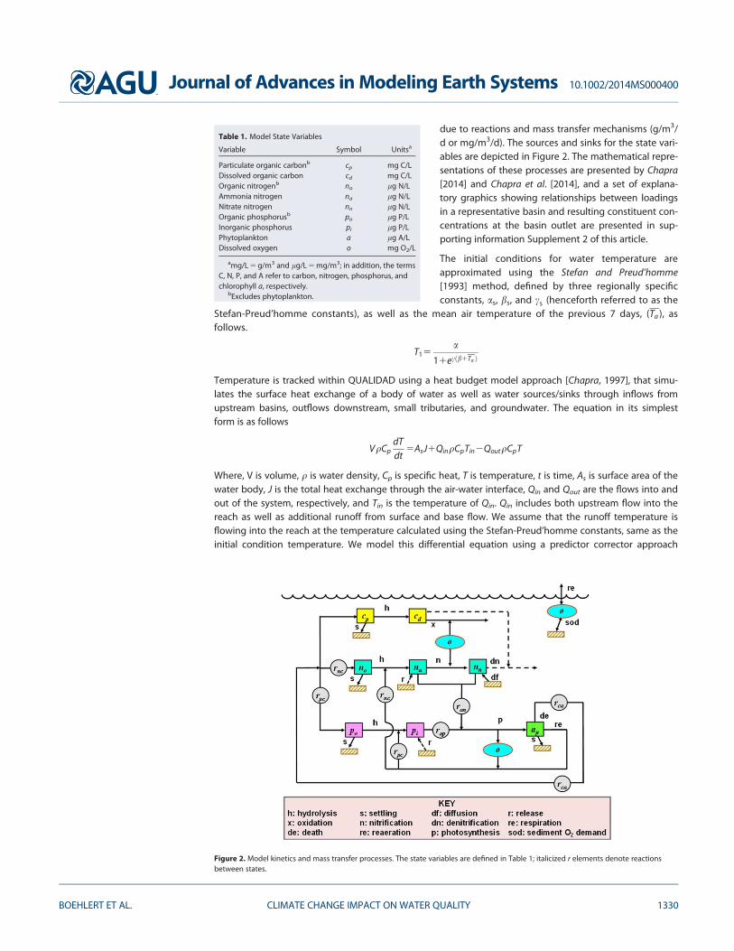
due to reactions and mass transfer mechanisms (g/m3/d or mg/m3/d). The sources and sinks for the state vari-ables are depicted in Figure 2. The mathematical repre-sentations of these processes are presented by Chapra[2014] and Chapra et al. [2014], and a set of explana-tory graphics showing relationships between loadingsin a representative basin and resulting constituent con-centrations at the basin outlet are presented in sup-porting information Supplement 2 of this article.

The initial conditions for water temperature areapproximated using the Stefan and Preud’homme[1993] method, defined by three regionally specificconstants, as, bs, and cs (henceforth referred to as the

Stefan-Preud’homme constants), as well as the mean air temperature of the previous 7 days, (Ta ), asfollows.

T15a

11ecðb1Ta Þ

Temperature is tracked within QUALIDAD using a heat budget model approach [Chapra, 1997], that simu-lates the surface heat exchange of a body of water as well as water sources/sinks through inflows fromupstream basins, outflows downstream, small tributaries, and groundwater. The equation in its simplestform is as follows

VqCpdTdt

5AsJ1QinqCpTin2QoutqCpT

Where, V is volume, q is water density, Cp is specific heat, T is temperature, t is time, As is surface area of thewater body, J is the total heat exchange through the air-water interface, Qin and Qout are the flows into andout of the system, respectively, and Tin is the temperature of Qin. Qin includes both upstream flow into thereach as well as additional runoff from surface and base flow. We assume that the runoff temperature isflowing into the reach at the temperature calculated using the Stefan-Preud’homme constants, same as theinitial condition temperature. We model this differential equation using a predictor corrector approach

Table 1. Model State Variables

Variable Symbol Unitsa

Particulate organic carbonb cp mg C/LDissolved organic carbon cd mg C/LOrganic nitrogenb no lg N/LAmmonia nitrogen na lg N/LNitrate nitrogen nn lg N/LOrganic phosphorusb po lg P/LInorganic phosphorus pi lg P/LPhytoplankton a lg A/LDissolved oxygen o mg O2/L

amg/L 5 g/m3 and lg/L 5 mg/m3; in addition, the termsC, N, P, and A refer to carbon, nitrogen, phosphorus, andchlorophyll a, respectively.

bExcludes phytoplankton.

Figure 2. Model kinetics and mass transfer processes. The state variables are defined in Table 1; italicized r elements denote reactionsbetween states.



outlined in MacCormack [1969], which has the advantage of stability and is not plagued by numericaldispersion.

In the summer, as temperature warms and solar radiation increases, stratification in temperate reservoirsoccurs. Temperature during the season of stratification is modeled differently for reservoirs, where a two-layer model is used, representing both the epilimnion (top) and the hypolimnion (bottom) layers. For exam-ple, if the reservoir is bottom releasing (i.e., outflow is occurring in the hypolimnion), then the following isused to model the reservoir temperature [Chapra, 1997].

VeqCpdTe

dt5AsJ1QinqCpTin1vt AtqCp Th2Teð Þ

VhqCpdTh

dt52QoutqCpTe1vt AtqCpðTe2ThÞ

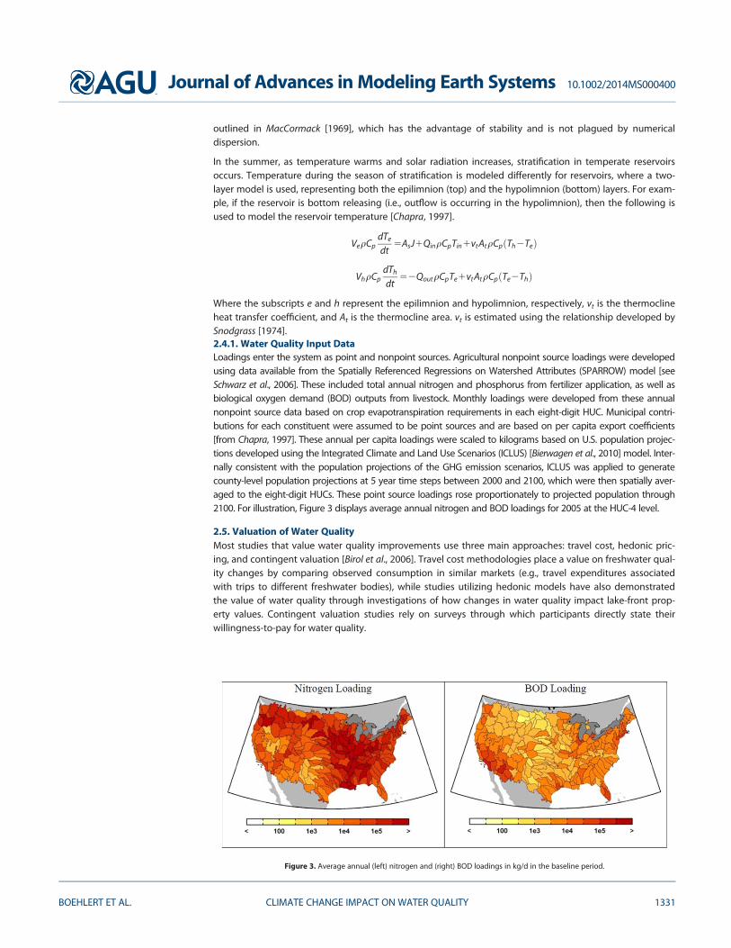
Where the subscripts e and h represent the epilimnion and hypolimnion, respectively, vt is the thermoclineheat transfer coefficient, and At is the thermocline area. vt is estimated using the relationship developed bySnodgrass [1974].2.4.1. Water Quality Input DataLoadings enter the system as point and nonpoint sources. Agricultural nonpoint source loadings were developedusing data available from the Spatially Referenced Regressions on Watershed Attributes (SPARROW) model [seeSchwarz et al., 2006]. These included total annual nitrogen and phosphorus from fertilizer application, as well asbiological oxygen demand (BOD) outputs from livestock. Monthly loadings were developed from these annualnonpoint source data based on crop evapotranspiration requirements in each eight-digit HUC. Municipal contri-butions for each constituent were assumed to be point sources and are based on per capita export coefficients[from Chapra, 1997]. These annual per capita loadings were scaled to kilograms based on U.S. population projec-tions developed using the Integrated Climate and Land Use Scenarios (ICLUS) [Bierwagen et al., 2010] model. Inter-nally consistent with the population projections of the GHG emission scenarios, ICLUS was applied to generatecounty-level population projections at 5 year time steps between 2000 and 2100, which were then spatially aver-aged to the eight-digit HUCs. These point source loadings rose proportionately to projected population through2100. For illustration, Figure 3 displays average annual nitrogen and BOD loadings for 2005 at the HUC-4 level.

2.5. Valuation of Water QualityMost studies that value water quality improvements use three main approaches: travel cost, hedonic pric-ing, and contingent valuation [Birol et al., 2006]. Travel cost methodologies place a value on freshwater qual-ity changes by comparing observed consumption in similar markets (e.g., travel expenditures associatedwith trips to different freshwater bodies), while studies utilizing hedonic models have also demonstratedthe value of water quality through investigations of how changes in water quality impact lake-front prop-erty values. Contingent valuation studies rely on surveys through which participants directly state theirwillingness-to-pay for water quality.

Figure 3. Average annual (left) nitrogen and (right) BOD loadings in kg/d in the baseline period.



Other efforts have used meta-analyses of multiple contingent valuation studies to create valuation modelsfor water quality improvements. For example, Van Houtven et al. [2007] use 131 willingness-to-pay estimatesfrom 18 studies to construct a meta-regression analysis, while Johnston et al. [2005] conduct a similar meta-analysis using 81 observations from 34 studies. More recently, Ge et al. [2013] use such a valuation model toestimate that a typical household in Iowa has a willingness-to-pay of $138 for a water quality increase from40 to 50 (out of 100) at a 2.6 km2 aquatic site. By linking these valuation models to water quality indices, theeconomic benefits (or costs) of changes in water quality can be estimated across a wide range of scenariosand locations.

In this study, the economic impacts of changes in water quality measures are estimated using a valuation ofchanges in the 10-point Water Quality Index (WQI10).The WQI was first developed and applied by theNational Sanitation Foundation (NSF) and explained in detail in McClelland [1974]. We develop WQI follow-ing a similar approach outlined by the U.S. Environmental Protection Agency [2009], which follows threesteps: (1) obtain measurements on water quality constituents, obtained directly from the water qualitymodel previously described, (2) convert each measurement into a subindex using water quality curves, and(3) aggregate the subindex values into the WQI. McClelland [1974] provides water quality curves (step 2)and aggregation weights (step 3) for nine water quality parameters. Four of these parameters coincide withoutput developed by the water quality model used in this study—namely, DO, Nitrates, Phosphates, andTemperature. Although quality curves can vary by location, we use the arithmetic mean for all basins. Wealso use the multiplicative form of the WQI aggregation, as suggested by McClelland [1974], redistributingthe weights of these five parameters to equal 1.

In order to model the relationship between changes in WQI and changes in Willingness-to-Pay (WTP)—used here as an indicator of economic costs and/or benefits—we use the reported values from the full lin-ear meta-regression transfer function from Van Houtven et al. [2007] to develop a piecewise linear functionfor both users and nonusers. We use state-level data from the U.S. Census Bureau [2014] on persons perhousehold to convert WTP per household to WTP per person and use the population projections used toestimate municipal and industrial water demands to develop a national WTP across scenarios and eras. VanHoutven et al. [2007] also distinguish costs by users and nonusers. We use state-level boating survey data[U.S. Coast Guard, 2012] to weight each eight-digit HUC by fraction of users and nonusers. The constituentvalues in each segment are averaged, weighting by segment surface area. Consequently, we are assumingthat each unit area is of equal importance.

3. Results

In the following section, we present the resulting constituent values for the control scenario as well as thechanges from the control to the three GHG emission scenarios. Then, the valuation results are presented interms of the differences between the REF and the Policy 3.7 and Policy 4.5 scenarios, which represent thebenefits of global GHG mitigation. The results presented are based on the year between 1980 and 2009with median level of mean annual runoff, selected for each hydrologically independent U.S. basin.

3.1. Baseline Water QualityFigure 4 shows the baseline annual average of four constituents output by the water quality model: temper-ature, total nitrogen, total phosphorus, and DO. Water temperatures for the baseline range from about 38Cto 238C, with warmer temperatures in the southern HUCs and colder temperatures in north and around themountainous west. Total nitrogen and total phosphorus concentrations vary across the country governedmostly by a ratio of loading over streamflow, with higher concentrations in drier western U.S. DO levels aregenerally higher in the West, and lower DO around the midwest and the coastal southwest.

3.2. Effect of Mitigation on Water QualityWe next evaluate the effects of global GHG mitigation on water quality by comparing changes projectedunder the REF scenario to changes under the mitigation scenarios. Figure 5 shows the difference in temper-ature change between the REF and both the Policy 3.7 and Policy 4.5 scenario in 2100, where negative val-ues indicate that the specified Policy results in lower river temperatures than the REF scenario. Changes inwater body temperature under the Policy 3.7 scenario compared to the REF range from a reduction ofapproximately 28C in the majority of the country, to more than 48C in the inland west. In the Policy 4.5 case,



changes in water body temperatures are lower in absolute value, especially in the inland west where wesee the greatest benefit of the more stringent mitigation policy.

Similarly, Figure 6 shows the relative change, as a percent of the baseline, between the total 2100 nitrogenconcentrations in REF and the two policy scenarios. Again, a negative value means that the specified policyreduces total nitrate concentrations. As shown, mitigation generally results in lower total nitrogen concen-trations compared to REF, especially in the midwest and eastern regions of the U.S. We see a very similarpattern for changes in total phosphorus concentration. Figure 7 shows the same results for the effect of mit-igation on DO concentrations, which show clear improvements under GHG mitigation, especially in thewest, owing largely to the effect of lower temperatures on oxygen saturation levels.

Figure 4. Four maps of constituents over the baseline period: (top left) temperature, (top right) total nitrates, (bottom left) phosphates,and (bottom right) dissolved oxygen.

Figure 5. Change in temperature (8C), where REF temperature change is subtracted from the (left) Policy 3.7 and (right) Policy 4.5 tempera-ture change in 2100 for the four seasons.



It is important to note that given the complex nature of this nested modeling system, interactions acrossspace, time, and within and between modeling components can produces a sometimes-counterintuitivepatchwork of basin and scenario-specific water quality and mitigation results, such as those observed in Fig-ure 7. For example, mitigation generally produces lower air temperatures, and yet there are many basins inFigure 7 where mitigation causes DO to decrease. Similarly, the sign of the effect of mitigation on DO oftendiffers between the Policy 3.7 and Policy 4.5 scenarios (e.g., in southern Florida, mid-Atlantic, Maine),although they are both mitigation scenarios from a common GCM. In these instances, the effects of mitiga-tion on DO are driven by a combination of changes in air temperature, basin-specific changes in river flows,resulting adjustments in reservoir management, and changes in concentrations of BOD. Unlike the uni-formly positive effect on air temperatures, the effect of climate change on precipitation and runoff patterns

Figure 6. Percent change in Total Nitrogen from REF for (left) Policy 3.7 and (right) Policy 4.5 in 2100.

Figure 7. Percent change in Dissolved Oxygen from REF for (left) Policy 3.7 and (right) Policy 4.5 in 2100.

Figure 8. Percent change in WQI from REF for (left) Policy 3.7 and (right) Policy 4.5.



is highly variable across both space and emissions scenario. Reduced river runoff will cause increased watertemperatures, higher concentrations of BOD given constant upstream loadings, and warmer upstream res-ervoir temperatures. Thus, the positive effects of the lower air temperatures are often offset by the negativeeffects of increased BOD concentrations and lower river flows. Similar basin and scenario-specific patternsof change can be observed in the percent change in total nitrogen presented in Figure 6.

3.3. ValuationIn this section, we apply the valuation scheme presented previously to the output of each water qualityconstituent to obtain a WTP value in 2005 USD. Figure 8 shows the annual benefit of GHG mitigation forboth policies as a percent change in the WQI. As the WQI was used to aggregate four water quality meas-ures shown previously into a unitless index, this map shows the overall change in the WQI across the four-digit HUCs of CONUS. The reduced emissions under the Policy scenarios increases WQI from between 3%and 30% compared to REF. The larger changes in WQI are mostly in the west where drier and hotter condi-tions are projected, and the largest effects of the more stringent mitigation policy, Policy 3.7, are in thesouthwest.

Table 2. National Average of the Annual Costs (i.e., Decreases in WTP) in 2050 and 2100 for Each Scenario

Control CS3-REF CS3-pol3.7 CS3-pol4.5 CS6-REF CS6-pol3.7

Mil 2005 USD 2050 $563 $1436 $841 $1202 $2060 $12762100 $928 $4060 $1506 $1953 $5522 $2224

USD/Person 2050 $1.10 $2.80 $1.64 $2.34 $4.02 $2.492100 $1.53 $6.67 $2.47 $3.21 $9.07 $3.65

Figure 9. Costs (decreases in WTP) of each era and scenario in USD/person/year.



Table 2 shows the national average annual costs for the control scenario (future population with historicalclimate conditions), CS3 REF, Policy 3.7 and Policy 4.5, as well as CS6 REF and Policy 3.7 in both 2050 and2100. Figure 9 shows maps of these values over the 18 two-digit HUCs. The difference between the GHGmitigation scenarios and the REF scenario is much higher in 2100, where WTP differences are about $2.5 bil-lion for Policy 3.7 and about $2 billion for Policy 4.5, resulting in a total present value benefit of approxi-mately $17.5 billion and $10.7 billion, respectively, using a 3% discount rate. As present value calculationsrequire a time series of annual values, this calculation assumes a linear increase in GHG mitigation benefitsfrom $0 in 2015 to the 2050 annual estimate between 2015 and 2050, and then another linear increasefrom the 2050 to 2100 value. In the map, we find that the larger costs in the REF are in the West, where hot-ter and drier conditions are projected, as compared to the East where increases in runoff often offsetdecreases in water quality. The southeast also shows large costs under the REF, which is partly driven by thelarger percentage of the population involved in recreational boating.

4. Conclusions and Further Research

In this study, we have linked a network of models to assess the benefits of global-scale GHG mitigation onwater quality in the contiguous U.S. The analysis runs changes in climate through a water resources systemsmodel, which drives a water quality model that ultimately estimates changes in temperature and constitu-ent concentrations of water bodies. Finally, valuation is used to aggregate four water quality constituentsinto a single metric, WQI, which is then used to estimate a benefit of GHG mitigation associated with WTPfor recreational water use. To our knowledge, such a U.S.-wide nested modeling framework has never previ-ously been developed at this level of detail to evaluate the full analytical chain of effects leading from cli-mate change projections, to supply/demand effects, to water quality implications, to the economic benefitsof GHG mitigation. Not surprisingly, we find that water temperatures increase substantially by 2100 in REF,but much less so under the Policy 4.5 and Policy 3.7. DO levels are mostly lower in the REF than Policy 3.7,although this varies across the country. The valuation results show that the overall benefit of GHG mitiga-tion is substantial, at a present value of $17.5 billion for Policy 3.7, discounted at 3%.

Like all current studies on climate change impacts, we are limited by the resolution and confidence levels ofsimulated climate data from GCMs. In this regard, using projections from only one GCM, the IGSM-CAMdoes not address uncertainties caused by assumptions inherent in GCM model structure. Also, note that theIGSM-CAM model projects a relatively ‘‘wet’’ future, i.e., precipitation and runoff increases are large overCONUS as compared to other GCMs [see Strzepek et al., 2014]. Lower relative runoff in the future would leadto higher concentrations of contaminants (i.e., less dilution), and therefore more potential for mitigationbenefit, suggesting that the results of this study are most likely conservative. It is also important to acknowl-edge the cascading errors that occur when employing nested models. The modeling framework employedin this study relies on a climate model, rainfall-runoff and water demand models, a water systems model, awater quality model, and a valuation model. To appropriately capture the uncertainty in such a frameworkwould require a Monte-Carlo simulation or another technique that samples from assumed input probabilitydistributions to develop a distribution of possible outputs.

Further research would evaluate a broader range of models and emissions scenarios to better capture therange of effects projected under climate change, providing a more appropriate risk portfolio for policy deci-sions. We are also limited by the accuracy of the WQI index used to aggregate the overall effect on water qual-ity, including the WTP estimates. While WQI is widely used, the quality curves used to translate model outputvalues into a common index are the same for all CONUS regions, whereas these relationships will likely varyacross the country. Similarly, we use a constant relationship between WTP and changes WQI. Future researchwould disaggregate these relationships to include differences in public opinion on the importance of waterpurity as well as household income, both of which impact the resulting WTP estimates. These modeled WTPestimates could also be compared to observed site-specific values for water quality improvements.

ReferencesAllen, R. G., L. S. Pereira, D. Raes, and M. Smith (1998), Crop evapotranspiration—Guidelines for computing crop water requirements, FAO

Irrig. Drain. Pap. 56, Food and Agric. Organ., Rome.Bierwagen, B. G., D. M. Theobald, C. R. Pyke, A. Choate, P. Groth, J. V. Thomas, and P. Morefield (2010), National housing and impervious sur-

face scenarios for integrated climate impact assessments, Proc. Natl. Acad. Sci. U. S. A., 107(49), 20,887–20,892.

AcknowledgmentsWe acknowledge the financial supportof the U.S. Environmental ProtectionAgency’s (EPA’s) Climate ChangeDivision (contract #EP-D-09–054) andaccess to reservoir data sets from theU.S. Army Corps of Engineers.Technical contributions were providedby Nicolas Tyack, Lisa Rennels, andAndrzej Strzepek. Data used toproduce the results of this paper canbe made available through thecorresponding author, Brent Boehlert,at [email protected].



Birol, E., K. Karousakis, and P. Koundouri (2006), Using economic valuation techniques to inform water resources management: A surveyand critical appraisal of available techniques and an application, Sci. Total Environ., 365, 105–122.

Bouwes, N. W., and R. Schneider (1979), Procedures in estimating benefits of water quality change, Am. J. Agric. Econ., 61, 535–539.Boyle, K. J., S. R. Lawson, H. J. Michael, and R. Bouchard (1998), Lakefront property owners’ economic demand for water clarity in Maine

lakes, Misc. Rep. 410, Univ. of Maine, Orono.Chapra, S. C. (1997), Surface Water-Quality Modeling, McGraw-Hill, N. Y.Chapra, S. C. (2007), Applied Numerical Methods With MATLAB for Engineering and Science, 2nd ed., McGraw-Hill, N. Y.Chapra, S. C. (2014), QUALIDAD: A Parsimonious Modeling Framework for Simulating River Basin Water Quality, Version 1.1, Documentation

and Users Manual, Civ. and Environ. Eng. Dep., Tufts Univ., Medford, Mass.Chapra, S. C., and R. P. Canale (2006), Numerical Methods for Engineers, 5th ed., McGraw-Hill, N. Y.Chapra, S. C., K. Flynn, and J. Rutherford. (2014), Parsimonious model for assessing nutrient impacts on periphyton-dominated streams,

J. Environ. Eng., 140(6), 04014014.Droogers, P., and R. Allen (2002), Estimating reference evapotranspiration under inaccurate data conditions, Irrig. Drain. Syst., 16, 33–45.Farmer, W. H., and R. M. Vogel (2012), Performance-weighted methods for estimating monthly streamflow at ungagged sites, J. Hydrol.,

477, 240–250.Ge, J., C. Kling, and J. Herriges (2013), How much is clean water worth? Valuing water quality improvement using a meta analysis, Working

Pap. 13016, Iowa State Univ., Dep. of Econ., Ames.Georgakakos, A., P. Fleming, M. Dettinger, C. Peters-Lidard, T. C. Richmond, K. Reckhow, K. White, and D. Yates (2014), Water resources, in

Climate Change Impacts in the United States: The Third National Climate Assessment, edited by J. M. Melillo, T. C. Richmond, andG. W. Yohe, chap. 3, pp. 69–112, U.S. Global Change Res. Program, Washington, D. C.

Gupta, V., and S. Sorooshian (1983), Uniqueness and observability of conceptual rainfall-runoff model parameters: The percolation processexamined, Water Resour. Res., 19(1), 269–276, doi:10.1029/WR019i001p00269.

Gupta, V., and S. Sorooshian (1985), The relationship between data and the precision of parameter estimates of hydrologic models, J.Hydrol., 81, 57–77.

Johnston, R. J., E. Y. Besedin, R. Iovanna, C. J. Miller, R. F. Wardwell, and M. H. Ranson (2005), Systematic variation in willingness to pay foraquatic resource improvements and implications for benefit transfer: A meta-analysis, Can. J. Agric. Econ., 53, 221–248.

Kaczmarek, Z. (1993), Water balance model for climate impact analysis, Acta Geophys. Polonica, 41(4), 1–16.Kaushal, S. S., G. E. Likens, N. A. Jaworski, M. L. Pace, A. M. Sides, D. Seekell, K. T. Belt, D. H. Secor, and R. L. Wingate (2010), Rising stream

and river temperatures in the United States, Frontiers Ecol. Environ., 8, 461–466, doi:10.1890/090037.Kenny, J. F., N. L. Barber, S. S. Hutson, K. S. Linsey, J. K. Lovelace, and M. A. Maupin (2009), Estimated use of water in the United States in

2005, U.S. Geol. Surv. Circ., 1344, 52 p.Leopold, L. B., and T. Maddock (1953), The hydraulic geometry channels and some physiographic implications, 57 pp., 252, U.S. Geol. Surv.

Prof. Pap., Washington, D. C.MacCormack, R. W. (1969), The effect of viscosity in hypervelocity impact cratering, Am. Inst. Aeronaut. Astronaut. Pap., 69, pp. 354.McClelland, N. I. (1974), Water quality index application in the Kansas River Basin, prepared for the U.S. Environmental Protection

Agency—Region 7, Rep. EPA-907/9–74-001, Kansas City, Missouri.Monier, E., J. R. Scott, A. P. Sokolov, C. E. Forest, and C. A. Schlosser (2013), An integrated assessment modeling framework for uncertainty

studies in global and regional climate change: The MIT IGSM-CAM (version 1.0), Geosci. Model Dev., 6, 2063–2085, doi:10.5194/gmd-6-2063-2013.

Monier, E., X. Gao, J. Scott, A. Sokolov, and A. Schlosser (2014), A framework for modeling uncertainty in regional climate change, Clim.Change, 131, 51–66, doi:10.1007/s10584-014-1112-5.

Paltsev, S., E. Monier, J. Scott, A. Sokolov, and J. Reilly (2013), Integrated economic and climate projections for impact assessment, Clim.Change, 131, 21–33, doi:10.1007/s10584-013-0892-3.

PRISM Climate Group (2014), Oregon State Univ., Corvallis. [Available at http://www.prism.oregonstate.edu.]Romero-Lankao, P., and J. B. Smith (2014), North America, in Climate Change 2014: Impacts, Adaptation, and Vulnerability, vol. 2, Regional

Aspects, edited by C. Field et al., chap. 26, Cambridge, Mass.Sahoo, G. B., and S. G. Schladow (2008), Impacts of climate change on lakes and reservoirs dynamics and restoration policies, Sustainability

Sci., 3, 189–199.Sahoo, G. B., S. G. Schladow, J. E. Reuter, and R. Coats (2011), Effects of climate change on thermal properties of lakes and reservoirs, and

possible implications, Stochastic Environ. Res. Risk Assess., 25, 445–456.Sahoo, G. B., S. G. Schladow, J. E. Reuter, R. Coats, M. Dettinger, J. Riverson, B. Wolfe, and M. Costa-Cabral (2012), The response of Lake

Tahoe to climate change, Clim. Change, 116, 71–95, doi:10.1007/s10584-012-0600-8.Schneider, P., and S. J. Hook (2010), Space observations of inland water bodies show rapid surface warming since 1985, Geophys. Res. Lett., 37, 1–5.Schwarz, G. E., A. B. Hoos, R. B. Alexander, and R. A. Smith (2006), The SPARROW surface water-quality model: Theory, application, and user

documentation, in U.S. Geological Survey Techniques and Methods, Book 6, chap. 3, sect. B, 248 pp., Reston, Va.Sheffield, J., G. Goteti, and E. F. Wood (2006), Development of a 50-year high-resolution global dataset of meteorological forcings for land

surface modeling, J. Clim., 19, 3088–3111.Short, W., P. Sullivan, T. Mai, M. Mowers, C. Uriarte, and N. Blair (2011), Regional Energy Deployment System (ReEDS), Contract, 303, 275–3000.Sieber, J., and D. Purkey (2007), User Guide for WEAP21, Stockholm Environ. Inst., Somerville, Mass.Snodgrass, W. J. (1974), A predictive phosphorus model for lakes: Development and testing, Ph.D. dissertation, Univ. of N. C., Chapel Hill.Stefan, H. G., and E. B. Preud’homme (1993), Stream temperature estimation from air temperature, Water Resour. Bull., 29(1), 27–45.Strzepek, K., A. McCluskey, B. Boehlert, M. Jacobsen, and C. Fant (2011), Climate variability and change: A basin scale indicator approach to

understanding the risk to water resources development and management, Water Pap. 67338, World Bank, Washington, D. C. [Availableat http://documents.worldbank.org/curated/en/2011/09/15897484/climate-variability-change-basin-scale-indicator-approach-under-standing-risk-water-resources-development-management.]

Strzepek, K., M. Jacobsen, B. Boehlert, and J. Neumann (2013), Toward evaluating the effect of climate change on investments in the waterresources sector: Insights from the forecast and analysis of hydrological indicators in developing countries, Environ. Res. Lett., 8(4),044014, doi:10.1088/1748-9326/8/4/044014.

Strzepek, K., et al. (2014), Benefits of greenhouse gas mitigation on the supply, management, and use of water resources in the UnitedStates, Clim. Change, 131, 127–141, doi:10.1007/s10584-014-1279-9.

U.S. Army Corps of Engineers (2013), National Inventory of Dams. [Available at http://nid.usace.army.mil/cm_apex/f?p=838:12.]U.S. Census Bureau (2014), American Community Survey 3-Year Estimates, Washington, D. C. [Available at http://factfinder2.census.gov.]



U.S. Coast Guard (2014), National Recreational Boating Survey, Washington, D. C. [Available at http://www.uscgboating.org/library/recrea-tional-boating-servey/2012survey%20report.pdf.]

U.S. Department of Agriculture (2010), Farm and Ranch Irrigation Survey (2008), vol. 3, Special Studies, Part 1, AC-07-SS-1, Washington, D. C.U.S. Environmental Protection Agency (2009), Environmental impact and benefits assessment for final effluent guidelines and standards

for the construction and development category, Rep. EPA-821-R-09-012, Off. of Water, Washington D. C.U.S. Forest Service (2014), Water Supply Stress Index (WaSSI), Asheville, N. C. [Available at http://www.forestthreats.org/research/tools/

WaSSI.]U.S. Geological Survey (1999), ERF1—Enhanced River Reach File 1.2, Reston, Va. [Available at http://water.usgs.gov/GIS/metadata/usgswrd/

XML/erf1.xml.]U.S. Water Resources Council (1978), The Nations Water Resources 1975–2000: Second National Water Assessment, Washington, D. C. [Avai-

lablr at http://water.usgs.gov/watercensus/nwr-1975-2000.html.]Van Houtven, G., J. Powers, and S. K. Pattanayak (2007), Valuing water quality improvements in the United States using meta-analysis: Is

the glass half-full or half-empty for national policy analysis?, Resour. Energy Econ., 29, 206–228.Van Houtven, G., C. Mansfield, D. J. Phaneuf, R. von Haefen, B. Milstead, M. A. Kenney, and K. H. Reckhow (2014), Combining expert elicita-

tion and stated preference methods to value ecosystem services from improved lake water quality, Ecol. Econ., 99, 40–52.Waldhoff, S., J. Martinich, M. Sarofim, B. DeAngelo, J. McFarland, L. Jantarasami, K. Shouse, A. Crimmins, S. Ohrel, and J. Li (2014), Overview

of the special issue: A multi-model framework to achieve consistent evaluation of climate change impacts in the United States, Clim.Change, 131, 1–20, doi:10.1007/s10584-014-1206-0.



MIT Joint Program on the Science and Policy of Global Change - REPRINT SERIESFOR THE COMPLETE LIST OF REPRINT TITLES: http://globalchange.mit.edu/research/publications/reprints

For limited quantities, Joint Program Reprints are available free of charge. Contact the Joint Program Office to order.

2014-22 Emissions trading in China: Progress and prospects, Zhang, D., V.J. Karplus, C. Cassisa and X. Zhang, Energy Policy, 75(December): 9–16 (2014)

2014-23 The mercury game: evaluating a negotiation simulation that teaches students about science-policy interactions, Stokes, L.C. and N.E. Selin, Journal of Environmental Studies & Sciences, online first (doi:10.1007/s13412-014-0183-y) (2014)

2014-24 Climate Change and Economic Growth Prospects for Malawi: An Uncertainty Approach, Arndt, C., C.A. Schlosser, K.Strzepek and J. Thurlow, Journal of African Economies, 23(Suppl 2): ii83–ii107 (2014)

2014-25 Antarctic ice sheet fertilises the Southern Ocean, Death, R., J.L.Wadham, F. Monteiro, A.M. Le Brocq, M. Tranter, A. Ridgwell, S. Dutkiewicz and R. Raiswell, Biogeosciences, 11, 2635–2644 (2014)

2014-26 Understanding predicted shifts in diazotroph biogeography using resource competition theory, Dutkiewicz, S., B.A. Ward, J.R. Scott and M.J. Follows, Biogeosciences, 11, 5445–5461 (2014)

2014-27 Coupling the high-complexity land surface model ACASA to the mesoscale model WRF, L. Xu, R.D. Pyles, K.T. Paw U, S.H. Chen and E. Monier, Geoscientific Model Development, 7, 2917–2932 (2014)

2015-1 Double Impact: Why China Needs Separate But Coordinated Air Pollution and CO2 Reduction Strategies, Karplus, V.J., Paulson Papers on Energy and Environment (2015)

2015-2 Behavior of the aggregate wind resource in the ISO regions in the United States, Gunturu, U.B. and C.A. Schlosser, Applied Energy, 144(April): 175–181 (2015)

2015-3 Analysis of coastal protection under rising flood risk, Lickley, M.J., N. Lin and H.D. Jacoby, Climate Risk Management, 6(2014): 18–26 (2015)

2015-4 Benefits of greenhouse gas mitigation on the supply, management, and use of water resources in the United States, K. Strzepek et al., Climatic Change, online first (doi: 10.1007/s10584-014-1279-9) (2015)

2015-5 Modeling Regional Transportation Demand in China and the Impacts of a National Carbon Policy, Kishimoto, P.N., D. Zhang, X. Zhang and V.J. Karplus, Transportation Research Record 2454: 1-11 (2015)

2015-6 Impacts of the Minamata Convention on Mercury Emissions and Global Deposition from Coal-Fired Power Generation in Asia, Giang, A., L.C. Stokes, D.G. Streets, E.S. Corbitt and N.E. Selin, Environmental Science & Technology, online first (doi: 10.1021/acs.est.5b00074) (2015)

2015-7 Climate change policy in Brazil and Mexico: Results from the MIT EPPA model, Octaviano, C., S. Paltsev and A. Gurgel, Energy Economics, online first (doi: 10.1016/j.eneco.2015.04.007) (2015)

2015-8 Changes in Inorganic Fine Particulate Matter Sensitivities to Precursors Due to Large-Scale US Emissions Reductions, Holt, J., N.E. Selin and S. Solomon, Environmental Science & Technology, 49(8): 4834–4841 (2015)

2015-9 Natural gas pricing reform in China: Getting closer to a market system? Paltsev and Zhang, Energy Policy, 86(2015): 43–56 (2015)

2015-10 Climate Change Impacts on U.S. Crops, Blanc, E. and J.M. Reilly, Choices Magazine, 30(2): 1–4 (2015)

2015-11 Impacts on Resources and Climate of Projected Economic and Population Growth Patterns, Reilly, The Bridge, 45(2): 6–15 (2015)

2015-12 Carbon taxes, deficits, and energy policy interactions, Rausch and Reilly, National Tax Journal, 68(1): 157–178 (2015)

2015-13 U.S. Air Quality and Health Benefits from Avoided Climate Change under Greenhouse Gas Mitigation, Garcia-Menendez, F., R.K. Saari, E. Monier and N.E. Selin, Environ. Sci. Technol. 49(13): 7580−7588 (2015)

2015-14 Modeling intermittent renewable electricity technologies in general equilibrium models, Tapia-Ahumada, K., C. Octaviano, S. Rausch and I. Pérez-Arriaga, Economic Modelling 51(December): 242–262 (2015)

2015-15 Quantifying and monetizing potential climate change policy impacts on terrestrial ecosystem carbon storage and wildfires in the United States, Mills, D., R. Jones, K. Carney, A. St. Juliana, R. Ready, A. Crimmins, J. Martinich, K. Shouse, B. DeAngelo and E. Monier, Climatic Change 131(1): 163–178 (2014)

2015-16 Capturing optically important constituents and properties in a marine biogeochemical and ecosystem model, Dutkiewicz, S., A.E. Hickman, O. Jahn, W.W. Gregg, C.B. Mouw and M.J. Follows, Biogeosciences 12, 4447–4481 (2015)

2015-17 The feasibility, costs, and environmental implications of large-scale biomass energy, Winchester, N. and J.M. Reilly, Energy Economics 51(September): 188–203 (2015)

2015-18 Quantitative Assessment of Parametric Uncertainty in Northern Hemisphere PAH Concentrations, Thackray, C.P., C.L. Friedman, Y. Zhang and N.E. Selin, Environ. Sci. Technol. 49, 9185−9193 (2015)

2015-19 Climate change impacts and greenhouse gas mitigation effects on U.S. water quality, Boehlert, B., K.M. Strzepek, S.C. Chapra, C. Fant, Y. Gebretsadik, M. Lickley, R. Swanson, A. McCluskey, J.E. Neumann and J. Martinich, Journal of Advances in Modeling Earth Systems, 7(3): 1326–1338 (2015)

http://globalchange.mit.edu/research/publications/reprints

Climate change impacts and greenhouse gas … change impacts and greenhouse gas mitigation effects...

Documents

Transcript of Climate change impacts and greenhouse gas … change impacts and greenhouse gas mitigation effects...