Enter Climate Change Source: NASA Climate Change Cooperation.
Upload
truongthuyCategory
view
220download
5
4chapter
This chapter uses a global dynamic model to exam-ine the macroeconomic and financial consequences of policies to address climate change. Although these consequences can be rapid and wide-ranging, this chapter finds that the overall costs of mitigation could be minimized if policies are well designed and accepted by a broad group of countries.
Climate change is a potentially cata-strophic global externality and one of the world’s greatest collective action problems. The distribution of causes
and effects is highly uneven across countries and across generations. Enormous uncertainty surrounds existing estimates of future damages that may result from climate change, but these potential damages are to a considerable extent irreversible and may be catastrophic if global warming is unchecked. The costs of abating climate change also have a sunk component—that is, cannot be fully recovered—and are contingent on a multitude of factors, including the rate at which the global economy grows over the long term and the pace at which low-emis-sion technologies emerge and diffuse across the global economy. The discount rate chosen to
aggregate damages from climate change and the costs of abating them across generations also has important implications for how various policy options are weighed by policymakers.
The macroeconomic consequences of policies to abate climate change can be immediate and wide-ranging, particularly when these policies are not designed carefully. The promotion of biofuels provides a good example. Expansion of biofuel production in the United States and western Europe in recent years has pushed up food prices and boosted inflation, creating seri-ous problems for poor food-importing countries around the world and limiting the ability of cen-tral banks to ease monetary policy in response to recent financial turbulence. The main cause of these negative effects is the fact that advanced economies have placed trade restrictions on imports of biofuels, constraining the production of biofuels in lower-cost countries such as Brazil.�
This chapter focuses on examining the macroeconomic and financial implications, for the global economy and for individual countries, of policies to address climate change.� First, the chapter reviews available estimates of damages from climate change, illustrating the potentially significant benefits of abatement and highlighting the key variations among these estimates.� Next, the chapter briefly discusses the need for countries to adapt their ecological, social, and economic systems to climate change. The costs of such adaptation will have significant
�Production of biofuels also needs to be environmen-tally sustainable. For more details on biofuels, see the October �007 World Economic Outlook.
�This study builds on the review of climate change issues in the October �007 World Economic Outlook. For an analysis of the fiscal implications of climate change, see IMF (�008).
�Abatement is defined here as the reduction in green-house gas (GHG) emissions. This term is used inter-changeably with the term “mitigation.” Adaptation means adjustment to climate change.
��
Climate Change and the global eConomy
Note: This chapter was prepared by Natalia Tamirisa (team leader), Florence Jaumotte, Ben Jones, Paul Mills, Rodney Ramcharan, Alasdair Scott, and Jon Strand, under the guidance of Charles Collyns. Nikola Spatafora, Eduardo Borensztein, Douglas Laxton, Marcos Chamon, and Paolo Mauro also made significant contributions to the chapter. Warwick McKibbin, Ian Parry, and Kang Yong Tan served as consultants for the project. Angela Espiritu, Elaine Hensle, and Emory Oakes provided research assistance. Joseph Aldy (Resources for the Future), Fatih Birol (International Energy Agency), Kirk Hamilton (World Bank), Helen Mountford and Jan Cor-fee-Morlot (both Organization for Economic Cooperation and Development, OECD), Georgios Kostakos and Luis Jimenez-McInnis (both Executive Office of the Secre-tary-General, in the Secretariat of the United Nations), Robert Pindyck (Massachusetts Institute of Technology), and Nicholas Stern (London School of Economics) and his team commented on an earlier draft.

Chapter 4 Climate Change and the global eConomy
�
bearing on the estimates of potential losses from climate change, and macroeconomic policies and financial markets can play a role in reduc-ing these costs.
The main contribution of this chapter is its analysis of the macroeconomic and financial implications of alternative mitigation policies across countries, using a global dynamic macro-economic model. An effective mitigation policy must be based on setting a price path for the greenhouse gas (GHG) emissions that drive climate change. The overall costs of such carbon-pricing policies—a global carbon tax, a global cap-and-trade system, or a hybrid policy—could be moderate, provided the policies are well designed.• Carbon pricing should be credible and long
term. If it is, then even small and gradual increases in carbon prices will be sufficient to induce businesses and people to shift away from emission-intensive products and technologies.
• Carbon pricing should be global. It is not feasible to contain climate change unless all major GHG emitters start pricing their emissions.
• Carbon pricing should seek to equalize the price of GHG emissions across countries to maximize the efficiency of abatement. Emis-sions would then be reduced more where it is cheaper to do so.
• Carbon pricing should be flexible, allowing firms to adjust the amount of abatement in response to changes in economic conditions, to avoid excessive volatility in carbon prices. High carbon price volatility could augment mac-roeconomic volatility and generate spillovers across the world. Policy frameworks should also provide scope to adjust policy parameters in response to new scientific information and experiences with policy implementation.
• Carbon pricing should be equitable. No undue burdens should be put on countries least able to bear them.All in all, the analysis highlights the impor-
tance of carefully designing mitigation policies to take into account their macroeconomic and financial effects, and thereby to ensure the sus-
tainability of any future international agreement on climate change.�
how Will Climate Change affect economies?
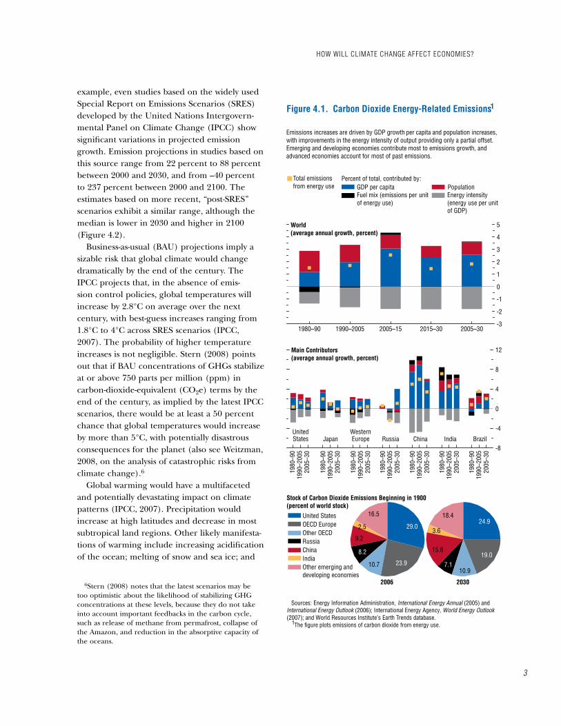
The global climate is projected to continue to warm in coming decades, as new GHG emissions augment the already large stock of past emis-sions. Increases in energy-related emissions of carbon dioxide, the largest and fastest-growing source of GHG emissions, are driven by growth in GDP per capita and increases in population, and these increases are only partially offset by improvements in the intensity of energy use (Figure �.�).� Catching-up economies, espe-cially large and fast-growing countries such as China and India, contribute most to the growth in emissions (Box �.�). Advanced economies account for most past energy-related emissions and thus for most of the current stock of these emissions. However, when changes in land use and deforestation are considered, a differ-ent conclusion emerges: advanced economies account for less than half of the current stock of total emissions (den Elzen and others, �00�; Baumert, Herzog, and Pershing, �00�).
outlook for Climate Change
Without changes in policy, GHG emissions are projected to accelerate. However, these projections are wide-ranging, given uncertainty about the rates at which productivity will grow, energy intensity will improve, and emerging and developing economies will converge toward the living standards of advanced economies. For
�Commitments under the central international agreement on emission levels—the Kyoto Protocol—are set to expire in �0��. At a recent conference in Bali, Indonesia, signatories to the United Nations Framework Convention on Climate Change (UNFCCC)—most of which are IMF members—agreed on the agenda for two years of negotiations on a new agreement, with a �009 deadline.
�Intensity of energy use is defined as energy use per unit of output and calculated as the ratio of total energy use to GDP.
�
example, even studies based on the widely used Special Report on Emissions Scenarios (SRES) developed by the United Nations Intergovern-mental Panel on Climate Change (IPCC) show significant variations in projected emission growth. Emission projections in studies based on this source range from �� percent to 88 percent between �000 and �0�0, and from –�0 percent to ��7 percent between �000 and ��00. The estimates based on more recent, “post-SRES” scenarios exhibit a similar range, although the median is lower in �0�0 and higher in ��00 (Figure �.�).
Business-as-usual (BAU) projections imply a sizable risk that global climate would change dramatically by the end of the century. The IPCC projects that, in the absence of emis-sion control policies, global temperatures will increase by �.8°C on average over the next century, with best-guess increases ranging from �.8°C to �°C across SRES scenarios (IPCC, �007). The probability of higher temperature increases is not negligible. Stern (�008) points out that if BAU concentrations of GHGs stabilize at or above 7�0 parts per million (ppm) in carbon-dioxide-equivalent (CO�e) terms by the end of the century, as implied by the latest IPCC scenarios, there would be at least a �0 percent chance that global temperatures would increase by more than �°C, with potentially disastrous consequences for the planet (also see Weitzman, �008, on the analysis of catastrophic risks from climate change).�
Global warming would have a multifaceted and potentially devastating impact on climate patterns (IPCC, �007). Precipitation would increase at high latitudes and decrease in most subtropical land regions. Other likely manifesta-tions of warming include increasing acidification of the ocean; melting of snow and sea ice; and
�Stern (�008) notes that the latest scenarios may be too optimistic about the likelihood of stabilizing GHG concentrations at these levels, because they do not take into account important feedbacks in the carbon cycle, such as release of methane from permafrost, collapse of the Amazon, and reduction in the absorptive capacity of the oceans.
1980
–90
1990
–200
520
05–3
0
1980
–90
1990
–200
520
05–3
0
1980
–90
1990
–200
520
05–3
0
1980
–90
1990
–200
520
05–3
0
1980
–90
1990
–200
520
05–3
0
1980
–90
1990
–200
520
05–3
0
1980
–90
1990
–200
520
05–3
0 -8
-4
0
4
8
12
1980–90 1990–2005 2005–15 2015–30 2005–30-3
-2
-1
0
1
2
3
4
5
GDP per capitaTotal emissionsfrom energy use Population
Fuel mix (emissions per unit of energy use)
Energy intensity(energy use per unitof GDP)
Percent of total, contributed by:
Figure 4.1. Carbon Dioxide Energy-Related Emissions
Emissions increases are driven by GDP growth per capita and population increases, with improvements in the energy intensity of output providing only a partial offset. Emerging and developing economies contribute most to emissions growth, and advanced economies account for most of past emissions.
World(average annual growth, percent)
1
Sources: Energy Information Administration, International Energy Annual (2005) and International Energy Outlook (2006); International Energy Agency, World Energy Outlook (2007); and World Resources Institute’s Earth Trends database. The figure plots emissions of carbon dioxide from energy use.
Stock of Carbon Dioxide Emissions Beginning in 1900(percent of world stock)
29.0
23.910.7
8.2
9.2
2.5
16.5United StatesOECD EuropeOther OECDRussiaChinaIndiaOther emerging anddeveloping economies
24.9
19.0
10.97.1
15.8
3.6
18.4
2006 2030
1
Main Contributors(average annual growth, percent)
UnitedStates Japan
WesternEurope Russia China India Brazil
how will Climate Change affeCt eConomies?

Chapter 4 Climate Change and the global eConomy
�
an increase in the intensity of extreme events such as heat waves, droughts, floods, and tropi-cal cyclones. At higher temperatures, the prob-ability of catastrophic climate changes would rise (for example, melting of the west Antarctic ice sheet or permafrost; a change in monsoon pat-terns in south Asia; or a reversal of the Atlantic Thermohaline Circulation, which would cool the climate of Europe).
economic Costs of Climate Change
Economic estimates of the impact of cli-mate change are typically based on “damage functions” that relate GDP losses to increases in temperature. The estimates of GDP costs embodied in the damage functions cover a variety of climate impacts that are usually grouped as market impacts and nonmarket impacts. Market impacts include effects on climate-sensitive sectors such as agriculture, for-estry, fisheries, and tourism; damage to coastal areas from sea-level rise; changes in energy expenditures (for heating or cooling); and changes in water resources. Nonmarket impacts cover effects on health (such as the spread of infectious diseases and increased water short-ages and pollution), leisure activities (sports, recreation, and outdoor activities), ecosystems (loss of biodiversity), and human settlements (specifically because cities and cultural heritage cannot migrate).
Existing studies tend to underestimate eco-nomic damages from climate change, particu-larly the risk of worse-than-expected outcomes. The three main benchmark studies (Men-delsohn and others, �000; Nordhaus and Boyer, �000; and Tol, �00�) and the review of the liter-ature in the Stern Review (�007) point to mean GDP losses between 0 percent and � percent of world GDP for a �°C warming (from �990–�000 levels) (Figure �.�).7 However, these estimates of damages are often incomplete—they rarely cover nonmarket damages, the risk of local
7See IPCC (�007) for a detailed review of the literature on damages.
1970 80 90 2000 SRES Post SRES Post0
40
80
120
160
200
240
Sources: EDGAR-HYDE 1.4 database; IPCC (2007); Netherlands Environmental Assessment Agency; Olivier and Berdowski (2001); Van Aardenne and others (2001); and IMF staff calculations. Global greenhouse gas emissions for 1970–2000 and projected baseline emissions for 2030 and 2100 are from the IPCC’s Special Report on Emissions Scenarios (SRES) and post-SRES literature. The figure shows emissions from the six illustrative SRES scenarios.
1
2030 2100
A1FI A2A1B AITB1 B2
SRES scenarios: Post-SRES estimates:5th to 95th percentile
MedianInterquartile range
Historical emissions
Figure 4.2. Emission Forecasts(Gigatons of carbon dioxide equivalent per year)
1
Emission forecasts cover a wide range of potential scenarios and outcomes, ranging from rapid output growth with developments of new energy technologies (the A1 scenario), less regional development convergence (A2), rapid shifts toward information- and services-based economies (B1), and fewer technological improvements (B2). All these scenarios are considered equally plausible, with no probabilities assigned to them. Even within each type of scenario, there is a wide range of emission projections (not shown), typically diverging by hundreds of percentage points by 2100.

�
extreme weather, socially contingent events, or the risk of large temperature increases and global catastrophes.8 Moreover, avail-able estimates tend to be based on a smaller increase in global temperatures than projected in the IPCC’s latest scenarios. Studies typi-cally calculate damages for a doubling of CO�e concentration from pre-industrial levels. Yet the latest IPCC’s BAU scenarios are expected to result in a tripling or quadrupling of concentra-tions by the end of the century, implying higher temperatures than those assumed in most studies. More recent, risk-based approaches to the analysis of damages from climate change point to significantly higher estimates than those suggested in the earlier literature (Stern, �008).
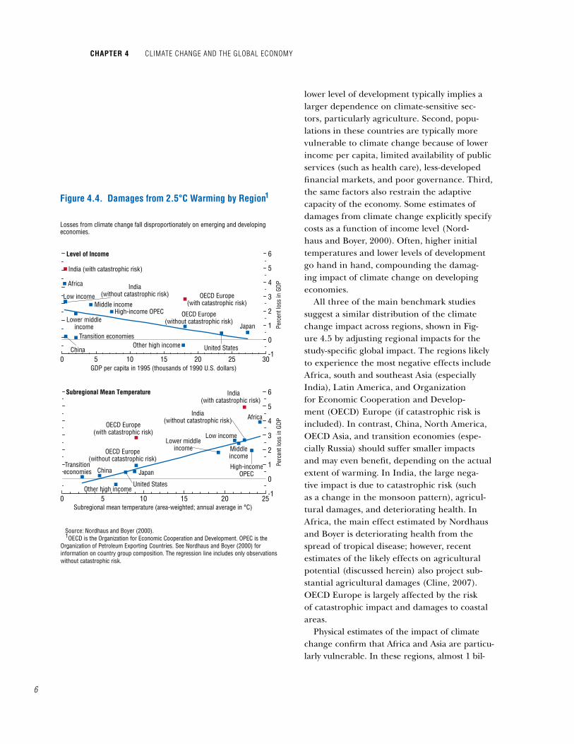
Estimates of total global damages also mask large variations across countries and regions. Damages tend to be greater for countries with higher initial temperatures, greater cli-mate change, and lower levels of development (Figure �.�). A moderate rise in temperature increases agricultural productivity in countries with low initial temperatures, but decreases it in hotter countries. Similarly, warming reduces deaths from cold in countries with initially colder climates, but increases mortality and morbidity in countries with warmer climates. Although warming reduces expenditures on win-ter heating in countries with an initially cooler climate, such countries may incur additional expenditures on summer cooling. Countries with initially warmer climates also incur addi-tional costs for cooling.
Beyond initial temperature, the level of development has a strong effect on the extent of damages from climate change. First, a
8Studies are also incomparable in methodology. Men-delsohn covers only market impacts; Tol covers market and nonmarket impacts; Nordhaus and Boyer and the Stern Review cover market and nonmarket impacts as well as catastrophic risks. The studies differ in their assump-tions about the extent of adaptation to climate change (large in Mendelsohn; smaller in Tol), and about the underlying economy (future or current). Mendelsohn’s estimates are based mostly on U.S. data and extrapolated for other countries.
0 1 2 3 4 5 6-12
-9
-6
-3
0
3
Source: Stern (2007). The studies presented in the Stern Review are from Mendelsohn, Schlesinger, andWilliams (2000), Nordhaus and Boyer (2000), and Tol (2002). Nordhaus and Boyer (2000) data adjusted for catastrophic risk are available only for2.5°C and 6°C. Observations were interpolated using a linear trend.
Global mean temperature increase (°C)
1
Mendelsohn
Nordhaus
Tol
Stern—high climate, market, and nonmarket impacts, and risk of catastrophe
Nordhaus—without catastrophic risk2
2
Figure 4.3. Mean GDP Losses at Various Levels of Warming
Estimates of GDP losses from climate change vary depending on the methodology and coverage of impacts and risks. GDP losses increase with temperature.
1
Perc
ent o
f wor
ld G
DP
how will Climate Change affeCt eConomies?
Chapter 4 Climate Change and the global eConomy
�
lower level of development typically implies a larger dependence on climate-sensitive sec-tors, particularly agriculture. Second, popu-lations in these countries are typically more vulnerable to climate change because of lower income per capita, limited availability of public services (such as health care), less-developed financial markets, and poor governance. Third, the same factors also restrain the adaptive capacity of the economy. Some estimates of damages from climate change explicitly specify costs as a function of income level (Nord-haus and Boyer, �000). Often, higher initial temperatures and lower levels of development go hand in hand, compounding the damag-ing impact of climate change on developing economies.
All three of the main benchmark studies suggest a similar distribution of the climate change impact across regions, shown in Fig-ure �.� by adjusting regional impacts for the study-specific global impact. The regions likely to experience the most negative effects include Africa, south and southeast Asia (especially India), Latin America, and Organization for Economic Cooperation and Develop-ment (OECD) Europe (if catastrophic risk is included). In contrast, China, North America, OECD Asia, and transition economies (espe-cially Russia) should suffer smaller impacts and may even benefit, depending on the actual extent of warming. In India, the large nega-tive impact is due to catastrophic risk (such as a change in the monsoon pattern), agricul-tural damages, and deteriorating health. In Africa, the main effect estimated by Nordhaus and Boyer is deteriorating health from the spread of tropical disease; however, recent estimates of the likely effects on agricultural potential (discussed herein) also project sub-stantial agricultural damages (Cline, �007). OECD Europe is largely affected by the risk of catastrophic impact and damages to coastal areas.
Physical estimates of the impact of climate change confirm that Africa and Asia are particu-larly vulnerable. In these regions, almost � bil-
0 5 10 15 20 25-1
0
1
2
3
4
5
6Subregional Mean Temperature
Perc
ent l
oss
in G
DP
Source: Nordhaus and Boyer (2000). OECD is the Organization for Economic Cooperation and Development. OPEC is the Organization of Petroleum Exporting Countries. See Nordhaus and Boyer (2000) for information on country group composition. The regression line includes only observations without catastrophic risk.
1
India(with catastrophic risk)
OECD Europe(with catastrophic risk)
AfricaIndia(without catastrophic risk)
Low income
Middleincome
High-incomeOPEC
Lower middleincomeOECD Europe
(without catastrophic risk)
Japan
United StatesOther high income
ChinaTransitioneconomies
OECD Europe(with catastrophic risk)
India (with catastrophic risk)
Figure 4.4. Damages from 2.5°C Warming by Region1
0 5 10 15 20 25 30-1
0
1
2
3
4
5
6
Perc
ent l
oss
in G
DP
Level of Income
Africa India(without catastrophic risk)Low income
Middle incomeHigh-income OPEC
Lower middleincome
China
Transition economiesOther high income
OECD Europe(without catastrophic risk)
United States
Japan
Losses from climate change fall disproportionately on emerging and developing economies.
GDP per capita in 1995 (thousands of 1990 U.S. dollars)
Subregional mean temperature (area-weighted; annual average in °C)

�
lion people would experience shortages of water by �080, more than 9 million could fall victim to coastal floods, and many could face increased hunger (Figure �.�). Pacific island countries are perhaps the most immediately vulnerable among the poor countries, as even a small further rise in sea level would dramatically affect their environment.
Two main areas of uncertainty plague esti-mates of damages from climate change at all levels, as is reflected in the large variation in the present value of damages. The first is the limitation of current scientific knowledge about the physical and ecological processes underly-ing climate change. For example, there is only incomplete information about how rapidly GHG concentrations will grow in the future, how sensitive climate and biological systems will be to increased concentrations of GHGs, and where the “tipping points” are, beyond which cata-strophic climate events can occur.9
The second source of uncertainty relates to how best to quantify the economic impact of climate change. The magnitude of losses from climate change depends, for example, on how well people and firms adapt and at what cost, as well as on the extent to which technological innovation can reduce the impact. For exam-ple, health effects from the spread of tropical disease may be lower if the spread of malaria can be reduced. Similarly, losses in agricultural yields may be limited if heat- and drought-resistant crops can be developed. Conven-tional approaches to evaluating damage from climate change also tend to neglect dynamic macroeconomic linkages. Climate change is largely a supply-side shock, but it may have significant effects on trade, capital flows, and
9This has implications for measures of economic damage. For example, the effect of climate change on productivity in agriculture and forestry depends to a large extent on the magnitude of carbon fertilization effects (a process by which higher concentrations of carbon dioxide in the atmosphere could result in increased crop yields), which is not known with certainty. Recent downward revisions to carbon fertilization effects have led to higher estimates of diminished world agricultural potential (Cline, �007).
United States
OECD Europe
Japan
High-income OPEC
Other high income
Middle income
Lower middle income
Low income
Africa
-2 -1 0 1 2 3 4 5 6
Sources: Hope (2006a); Mendelsohn, Schlesinger, and Williams (2000); Nordhaus and Boyer (2000); and Tol (2002). Shows the median impact of the Ricardian and Reduced-Form models for a 2°C warming. South and southeast Asia includes Middle East and China. No data are available for Asian Organization for Economic Cooperation and Development (OECD) countries and high-income OPEC (Organization of Petroleum Exporting Countries) countries. Impact of a 1°C warming. High-income OPEC refers to the Middle East. China includes other centrally planned Asian economies. No data are available for transition economies. Impact of a 2.5°C warming. North America refers only to the United States. OECD Asia refers only to Japan. South and southeast Asia refers only to India. No data are available for Latin America. Shows the median impact of models with and without adaptation at 2.5°C warming. North America refers only to the United States. South and southeast Asia refers only to India. No data are available for OECD Asia and high-income OPEC countries. World impact is estimated as follows: Mendelsohn at 0.13, Tol at 2.30, Nordhaus at -1.50, and Hope at -1.15 percent of GDP. Estimates from Nordhaus and Boyer (2000).
1
2
3
4
5
GDP Loss by Region and Sector (percent)
India
World (populationweighted)
World
Other marketAgricultureOther nonmarketHealthCatastrophicNet effect
6
Figure 4.5. Impact of Warming by Region and Sector
Mendelsohn–at 2.0°C warmingTol–at 1.0°C warming
Hope–at 2.5°C warmingNordhaus–at 2.5°C warming
12
34
Africa, south and southeast Asia (especially India), Latin America, and European OECD countries are likely to be most affected by climate change.
United States
OECD Europe
Japan
High-income OPEC
Transition economies
Latin America
China
Africa
-8 -6 -4 -2 0 2 4
India
GDP Loss by Region (percentage point deviation from world impact)5
China
Transition economies
6
how will Climate Change affeCt eConomies?

Chapter 4 Climate Change and the global eConomy
�
migration, as well as on investment and savings (Box �.�).�0
Quantifying the aggregate losses across genera-tions involves use of a single welfare measure and bears on the present value estimates of global losses. The rate at which the welfare of future generations should be discounted to the pres-ent (which relates to the marginal product of capital) is the subject of considerable debate. The Stern Review’s estimate that climate change would produce a large welfare cost—equivalent to a permanent reduction in consumption of about �� percent of world output over the next two cen-turies—is much higher than the average annual estimated output loss.�� This reflects a low elastic-ity of marginal utility to consumption and an assumed pure rate of time preference of approxi-mately zero, both of which give a large weight to consumption losses from distant generations.�� Many consider these assumptions unpersuasive because they imply a much higher-than-observed savings rate and a lower-than-observed rate of return on capital (Nordhaus, �007a; and Dasgupta, �007). Stern (�008) points out that discount rates are conditional on the path of future growth in consumption, implying that a lower discount rate should apply in a world with climate change than in a world without it, all other things equal. He also underscores that basing discount rates on market rates is funda-mentally inappropriate in cases involving welfare trade-offs across far-apart generations and across countries with different levels of income. Tech-nological change (DeLong, �00�) and uncer-
�0For instance, as climate lowers output now and in the future, investment may fall because there are fewer resources to invest and because the rate of return on capi-tal is lower. Using simulations, Fankhauser and Tol (�00�) show that the capital accumulation effect is important, especially if technological change is endogenous, and may be larger than the direct impact of climate change.
��Under the Stern Review’s “high-climate scenario” with catastrophic, market, and nonmarket impacts, the mean losses are less than � percent of world output in �0�0, �.9 percent in ��00, and ��.8 percent in ��00.
��Raising the pure rate of time preference from 0.� to a still modest �.� reduces the range of expected damage costs from �–�0 percent to �.�–� percent of global con-sumption (see the October �007 World Economic Outlook).
-40
-30
-20
-10
0
10
20
-50
-40
-30
-20
-10
0
10Canada
Mexico
India
Increased Water Resource Stress(millions of people)
0
500
1000
1500
2000
2500
3000
3500
-40
-30
-20
-10
0
10
20
30
40
Euro
pe
Asia
North
Am
eric
aSo
uth
Amer
ica
Afric
a
Aust
rala
sia
Wor
ld
Euro
pe
Asia
North
Am
eric
aSo
uth
Amer
ica
Afric
a
Aust
rala
sia
Wor
ld
0
100
200
300
400
500
600 Increased Risk of Hunger without Carbon Fertilization (millions of people)
Increased Risk of Hunger with Maximum Carbon Fertilization (millions of people)
0
5
10
15
20
25
30
35 Increase in Additional Annual Number of Coastal Flood Victims(millions of people)
Figure 4.6. Physical Impact by 20801
Median
Minimum
Maximum
Physical estimates of climate change impact confirm that Asia and Africa are particularly vulnerable to climate change.
Change in Agricultural Potential (percent)2,3
Without Carbon Fertilization With Carbon Fertilization
Russia
China
Canada
UnitedStates
Brazil
Russia
ChinaUnitedStates
Brazil
India
Mexico
Sources: Cline (2007); and Yohe and others (2007). Data for panels 1–4 are from Yohe and others (2007); sample includes estimates from A1FI, A2, B1, and B2 Special Report on Emissions Scenarios (IPCC, 2007). Data for panels 5–6 are from Cline (2007). All impacts are measured relative to the situation in 2080 with no climate change. Regional compositions may not be comparable across panels. Carbon fertilization refers to the increase in crop productivity as a result of the effect of carbon dioxide on crops. Estimates without carbon fertilization are weighted averages of the estimates from a Ricardian model and crop models. Estimates with carbon fertilization include the effect of a uniform boost of 15 percent in yield. See Cline (2007) for more information.
1
2
2 2
3
Euro
pe
Asia
North
Am
eric
aSo
uth
Amer
ica
Afric
aAu
stra
lasi
a
Wor
ld
Euro
pe
Asia
North
Am
eric
aSo
uth
Amer
ica
Afric
aAu
stra
lasi
a
Wor
ld
Euro
pe
Asia
North
Am
eric
aSo
uth
Amer
ica
Afric
aAu
stra
lasi
a
Wor
ld
Euro
pe
Asia
North
Am
eric
aSo
uth
Amer
ica
Afric
aAu
stra
lasi
a
Wor
ld
�
tainty over future discount rates may also justify using lower discount rates (Pindyck, �007).
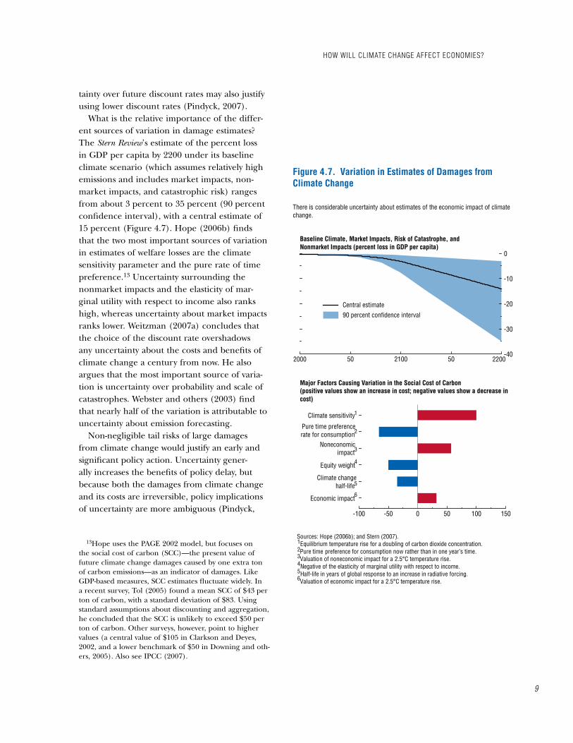
What is the relative importance of the differ-ent sources of variation in damage estimates? The Stern Review’s estimate of the percent loss in GDP per capita by ��00 under its baseline climate scenario (which assumes relatively high emissions and includes market impacts, non-market impacts, and catastrophic risk) ranges from about � percent to �� percent (90 percent confidence interval), with a central estimate of �� percent (Figure �.7). Hope (�00�b) finds that the two most important sources of variation in estimates of welfare losses are the climate sensitivity parameter and the pure rate of time preference.�� Uncertainty surrounding the nonmarket impacts and the elasticity of mar-ginal utility with respect to income also ranks high, whereas uncertainty about market impacts ranks lower. Weitzman (�007a) concludes that the choice of the discount rate overshadows any uncertainty about the costs and benefits of climate change a century from now. He also argues that the most important source of varia-tion is uncertainty over probability and scale of catastrophes. Webster and others (�00�) find that nearly half of the variation is attributable to uncertainty about emission forecasting.
Non-negligible tail risks of large damages from climate change would justify an early and significant policy action. Uncertainty gener-ally increases the benefits of policy delay, but because both the damages from climate change and its costs are irreversible, policy implications of uncertainty are more ambiguous (Pindyck,
��Hope uses the PAGE �00� model, but focuses on the social cost of carbon (SCC)—the present value of future climate change damages caused by one extra ton of carbon emissions—as an indicator of damages. Like GDP-based measures, SCC estimates fluctuate widely. In a recent survey, Tol (�00�) found a mean SCC of $�� per ton of carbon, with a standard deviation of $8�. Using standard assumptions about discounting and aggregation, he concluded that the SCC is unlikely to exceed $�0 per ton of carbon. Other surveys, however, point to higher values (a central value of $�0� in Clarkson and Deyes, �00�, and a lower benchmark of $�0 in Downing and oth-ers, �00�). Also see IPCC (�007).
Climate sensitivity
Equity weight
Economic impact
-100 -50 0 50 100 150
Noneconomicimpact
Pure time preferencerate for consumption
50 2100 50-40
-30
-20
-10
0
90 percent confidence intervalCentral estimate
Baseline Climate, Market Impacts, Risk of Catastrophe, andNonmarket Impacts (percent loss in GDP per capita)
2000
Major Factors Causing Variation in the Social Cost of Carbon(positive values show an increase in cost; negative values show a decrease in cost)
1
2
3
4
Climate changehalf-life 5
6
Sources: Hope (2006b); and Stern (2007). Equilibrium temperature rise for a doubling of carbon dioxide concentration. Pure time preference for consumption now rather than in one year’s time. Valuation of noneconomic impact for a 2.5°C temperature rise. Negative of the elasticity of marginal utility with respect to income. Half-life in years of global response to an increase in radiative forcing. Valuation of economic impact for a 2.5°C temperature rise.
123456
Figure 4.7. Variation in Estimates of Damages from Climate Change
There is considerable uncertainty about estimates of the economic impact of climate change.
2200
how will Climate Change affeCt eConomies?
Chapter 4 Climate Change and the global eConomy
�0
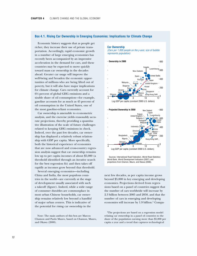
Economic history suggests that as people get richer, they increase their use of private trans-portation. Accordingly, rapid economic growth in a number of large emerging economies has recently been accompanied by an impressive acceleration in the demand for cars, and these countries may be expected to move quickly toward mass car ownership in the decades ahead. Greater car usage will improve the well-being and broaden the economic oppor-tunities of millions who are being lifted out of poverty, but it will also have major implications for climate change. Cars currently account for �½ percent of global GHG emissions and a sizable share of oil consumption—for example, gasoline accounts for as much as �� percent of oil consumption in the United States, one of the most gasoline-reliant economies.
Car ownership is amenable to econometric analysis, and the exercise yields reasonably accu-rate projections, thereby providing a quantita-tive illustration of the scale of future challenges related to keeping GHG emissions in check. Indeed, over the past few decades, car owner-ship has displayed a relatively robust relation-ship with GDP per capita. More specifically, both the historical experience of economies that are now advanced and cross-country regres-sion analysis suggest that car ownership remains low up to per capita incomes of about $�,000 (a threshold identified through an iterative search for the best regression fit) and then takes off rapidly as incomes grow beyond that threshold.
Several emerging economies—including China and India, the most populous coun-tries in the world—are currently at the stage of development usually associated with such a takeoff (figure). Indeed, while a wide range of consumer durables are commonplace in most urban Chinese households, car owner-ship remains relatively low beyond a handful of major urban centers. This is indicative of the potential for rising car ownership in the
next few decades, as per capita income grows beyond $�,000 in key emerging and developing economies. Projections derived from regres-sions based on a panel of countries suggest that the number of cars worldwide will increase by �.� billion between �00� and �0�0, and that the number of cars in emerging and developing economies will increase by �.9 billion.� Compa-
�The projections are based on a regression model relating car ownership in a panel of countries to the share of the population earning more than $�,000 per capita a year and a trend that captures technological
box 4.1. rising Car ownership in emerging economies: implications for Climate Change
Note: The main authors of this box are Marcos Chamon and Paolo Mauro, based on Chamon, Mauro, and Okawa (�008).
Car Ownership(Cars per 1,000 people on the y-axis; size of bubblerepresents population)
10 12Log GDP per capita (constant 2000 U.S. dollars)
Projected Ownership in 2050
Sources: International Road Federation, World Road Statistics; World Bank, World Development Indicators (2007); andprojections from Chamon, Mauro, and Okawa (2008).
800
600
400
200
0
ChinaIndia
Bulgaria
Canada
Chile
Spain
Ethiopia
United Kingdom
Hong Kong SAR
Israel
Japan
Korea
Luxembourg
Mexico
Malaysia
New Zealand
Portugal
Ukraine
Poland
Russia
Singapore
United States
4 6 8 10 12Log GDP per capita (constant 2000 U.S. dollars)
Ownership in 2000
800
600
400
200
0Ethiopia
Nigeria
Bangladesh
Pakistan
IndiaChina
Ukraine
Indonesia Russia
Hong Kong SAR
SingaporeIsrael Chile
MexicoKorea
MalaysiaPortugal
Bulgaria
Poland
New Zealand
Japan
UnitedStates
Canada
Spain
United Kingdom Luxembourg
Box 4.1. Figure 1
4 6 8
��
�007). The significant probability of climate catastrophes strengthens the case for earlier abatement—that is, reduction of GHG emis-sions—with abatement initiatives increasing in
intensity as learning progresses (Stern, �008; and Weitzman, �008). Even with aggressive abate-ment, however, it will be necessary to pursue adaptation—adjustments in ecological, social,
rable projections are supported by microecono-metric estimates based on two surveys of tens of thousands of households in China and India. The results confirm that as more and more households reach income levels that allow them to afford a car, ownership should rise by ½ bil-lion cars in China and !/3 billion cars in India between now and �0�0. The projected increase in car ownership in these emerging market giants (and other countries at a similar stage of development) will not only have substantial fiscal consequences for these countries—which are likely to require infrastructure investment to support such increased demand for transporta-tion—but will also have major implications for emissions and climate change.
A simple back-of-the-envelope calculation regarding GHG emissions may help gauge the implications of an increase in the worldwide car fleet from 0.� billion in �000 to �.9 billion in �0�0. According to the Stern Review (�007), cars (and vans) accounted for emissions equiva-lent to �.� gigatons of carbon dioxide (GtCO�) in �000. Relating the projected increase in the number of cars to additional emissions requires strong simplifying assumptions about future improvements in fuel efficiency. Over the past two and a half decades, the average number of miles per gallon has been broadly stable in most advanced economies, as technological improve-ments have been accompanied by increases in average car weight. Assuming that the growth rate of car emissions is the same as the growth rate of cars, worldwide emissions by cars would amount to �.8 GtCO� in �0�0. To put this in perspective, the Stern Review’s business-as-usual
improvements; long-term projections for economic growth are based on published sources. For more details on the methodology and sources, see Chamon, Mauro, and Okawa (�008).
scenario foresees that total emissions (flow) from all sources will rise from �� GtCO� in �000 to 8� GtCO� in �0�0. Emissions from cars as a share of total CO� emissions from all sources would thus rise from �.� percent in �000 to 8.� percent in �0�0. To sum up, cars could contribute significantly—and more than propor-tionately—to an increase in emissions from all sources that would have profound implications for climate change.
Policymakers in emerging and developing economies have an opportunity to “lean against the wind” of greater car ownership that inevi-tably results from economic development by promoting investment in appropriate subway, rail, and/or public transportation infrastruc-ture. Local pollution concerns also have become an important driver for policy change. The wide variation in gasoline taxes across countries—ranging from $0.� a gallon in the United States (and even less in some develop-ing economies) to more than $� a gallon in the United Kingdom—suggests that there may be significant room to increase fuel taxation in various parts of the world. Some countries also have begun to make substantial use of fuel efficiency standards. Notably, China introduced such standards in �00� and will make them more stringent in �008. At present, China’s fleet average fuel economy standards are more strict than those in Australia, Canada, and the United States, though somewhat less strict than those in Europe and Japan. Additional policy measures include higher taxes on less-fuel-efficient cars.
While such policies seem necessary, they are likely to be insufficient. Ultimately, much will depend on progress with respect to new technologies—such as plug-in hybrids or other breakthroughs that we are unable to fore-see—and incentives for innovation may also be considered in this area.
how will Climate Change affeCt eConomies?
Chapter 4 Climate Change and the global eConomy
��
This box presents some scenarios that illus-trate the economic effects on an open economy of an abrupt change in climate. This example examines the impact of changes in the mon-soon pattern on a representative south Asian country that is heavily reliant on agriculture, but the arguments are relevant to other coun-tries exposed to major climate shocks.
These scenarios were developed using a six-country� annual version of the Global Inte-grated Monetary and Fiscal Model (GIMF).� GIMF is a multicountry dynamic stochastic gen-eral equilibrium model that has been designed for multilateral surveillance. It includes strong non-Ricardian features whereby fiscal policies have significant real effects. It also includes significant nominal and real rigidities, mak-ing it a useful tool to study both the short- and long-term implications of supply and demand shocks.
Abrupt Climate Shock
The baseline climate change scenario, shown as the red lines in the leftmost column of the figure, assumes that a sudden and permanent deterioration in climate leads to failed har-vests and therefore higher mortality rates and emigration to neighboring countries. In the first year � percent of the population either perishes or emigrates, followed by 0.� percent a year over the subsequent five years, leading to a population decline of � percent over the long term.
In addition to the population effects, drastic changes in climate could also make obsolete many existing agricultural, distributional, and associated industrial patterns, forcing the relocation or decommissioning of existing
Note: The main authors of this box are Michael Kumhof and Douglas Laxton, with support from Susanna Mursula.
�The country blocks are emerging Asia, euro area, India, Japan, United States, and the remaining countries. Trade linkages among these countries were calibrated using the �00� matrix of world trade flows.
�For a description of the structure of the model see Kumhof and Laxton (�007).
capital stocks and the relocation or retrain-ing of labor. This represents a large shock to the stock of a country’s technology, which would likely result in a significant decline in total factor productivity.� For this south Asian economy, productivity growth would be significantly reduced over the medium term in both the tradable and the nontradable sectors of the economy. This would be accompanied by negative effects on foreign demand for the country’s products, due to reduced competi-tiveness in the new industries in which the country is forced to specialize.
Relative to baseline, these shocks cause an immediate � percent and ultimately more than 8 percent contraction in GDP, accompanied by a � percent real depreciation as domestic goods prices fall. Policy is accommodative, through both a lowering of interest rates and a deteriora-tion in the fiscal deficit.� Both measures reduce national savings and drive the current account into deficit.
Financial Market Response
The blue lines in the leftmost column of the figure show a scenario that adds to the direct climate-related shocks a risk premium shock of � percentage point a year, as financial markets respond to the country’s deteriorating performance and prospects. Higher interest rates reduce capital accumulation and there-fore GDP, which ultimately ends up � percent lower than in the baseline scenario. Because a higher risk premium raises domestic savings, it leads to depreciation of the real exchange
�For estimates of the long-run effects on productiv-ity see Nordhaus (�007b).
�Fiscal policy is assumed to target a structural interest-inclusive deficit consistent with the preex-isting stock of government debt, with the govern-ment’s estimate of the permanently sustainable tax base reduced only slowly in response to lower realized tax revenue. As a result, tax rates are raised only gradually when the economy contracts, result-ing in several years of deficits and increases in debt. Relative to a balanced budget rule, such a policy is expansionary.
box 4.2. South asia: illustrative impact of an abrupt Climate Shock

��
1 2 3 4 5 6 7 8 9 10-1
0
1
2
3
1 2 3 4 5 6 7 8 9 10-6
-4
-2
0
2
4
Source: IMF staff calculations. A positive value represents an appreciation relative to the baseline.
1 2 3 4 5 6 7 8 9 10-4
-3
-2
-1
0
1
2
3
Real Effective Exchange Rate (percent)
1 2 3 4 5 6 7 8 9 10-1.4
-1.2
-1.0
-0.8
-0.6
-0.4
-0.2
1 2 3 4 5 6 7 8 9 10-0.4
-0.2
0.0
0.2
0.4
0.6
0.8
1 2 3 4 5 6 7 8 9 10-1.0
-0.8
-0.6
-0.4
-0.2
0.0
0.2
0.4
0.6
Current Account/GDP (percentage points)
1 2 3 4 5 6 7 8 9 100
1
2
3
4
5
1 2 3 4 5 6 7 8 9 10-12
-10
-8
-6
-4
-2
0
1 2 3 4 5 6 7 8 9 10-12
-10
-8
-6
-4
-2
0
2GDP (percent)
Negative productivity andpopulation shock
Rapid fiscal response Combined effects withrapid fiscal response
Plus country risk-premium shockGradual fiscal response
Combined effects withgradual fiscal response
Illustrative Impact of Climate Change(Deviations from control; x-axis in years)
Direct Effects withoutGovernment Response
Effect ofGovernment Response
CombinedEffects
1
1
how will Climate Change affeCt eConomies?
Chapter 4 Climate Change and the global eConomy
��
rate in the short run and causes the current-account-to-GDP ratio to be around 0.7 percent-age point higher than in the baseline scenario. After a few years, the improving external asset position causes the real exchange rate to appreciate.
Government Response
Because sufficiently large climate shocks can cause a country’s stock of technology to deteriorate significantly, the question arises of how best to rebuild that technology. Clearly, the private sector will have a significant role to play, but private investment may be hampered by the disincentives to capital accumulation stemming from higher real interest rates. Fur-thermore, the affected economy would require a large-scale investment in public goods such as relief facilities to protect the population, rebuild transportation and communications infrastructure, and retrain the workforce. The middle column of the figure illustrates two such scenarios.�
The red lines show the incremental effects of an increase in public investment by �.� percent of GDP over a period of three years. This is financed by the issuance of additional govern-ment debt, which is allowed to increase by �0 percent of GDP in the long run, accompa-nied by a 0.� percent permanent increase in the government-deficit-to-GDP ratio from year four onward. The model assumes that private agents do not save sufficiently to offset such changes in public sector savings. This implies that the issuance of additional government debt crowds out private sector investment in other assets, in this case principally by reducing net foreign assets by 9 percent of GDP in the long run.
�It may be possible to phase in some public invest-ment ahead of a climate shock. But in order to be effective, this would require advance knowledge of exactly when and where such a shock will hit. Given the tremendous uncertainties associated with climate change, there would seem to be only limited scope for such preemptive action.
Higher public investment increases the stock of public capital by �� percent at the end of year three. The scenario predicts that GDP increases throughout, initially by about � percent as a result of increased government demand, and after a few years by about � per-cent because of the productivity-enhancing effects of a larger public capital stock.� The large increase in demand and corresponding decline in national savings causes an initial current account deficit of more than � percent of GDP and a � percent real appreciation. The current account remains negative as a result of permanently lower government savings, eventu-ally causing the real exchange rate to depreciate enough to generate an export volume sufficient to service the increased external debt.
A policy of rapid government investment may be necessary if the climate shock causes an especially dramatic collapse in activity at the outset. If it does not, as in our baseline scenario, then a more gradual approach may be in order. This is illustrated by the blue lines in the middle column of the figure, which show an increase of public investment by � percent of GDP over a period of �0 years. The effects on GDP are similar but are realized much more gradually. The differences are due to the different implica-tions of the two public investment scenarios on the cumulative public capital stock and on the effect of the rate of depreciation.
The red and blue lines in the rightmost column of the figure combine the climate change scenario, including the risk premium response, with either of the two public invest-ment scenarios. Public investment accomplishes two objectives: (�) mitigating the impact of the climate shock, which is most effective when the investment is concentrated in the period imme-diately following the shock, and (�) mitigating the long-run effects of the shock, which is most effective when the investment is spread over a longer time period.
�The elasticity of output with respect to public capital has been calibrated to be consistent with the empirical literature. See Ligthart and Suárez (�00�).
box 4.2 (concluded)
��
or economic systems in response to climatic impacts.�� If serious efforts to cut emissions were undertaken immediately, some climate warming would still occur, making adaptation unavoid-able. However, adaptation is an inadequate response on its own, because there are natural limitations to humans’ ability to adapt at higher degrees of warming.
how Can Countries best adapt to Climate Change?
Societies have historically adapted to chang-ing environmental conditions, and individuals and firms can be expected to continue altering their behavior in response to changing climate conditions (for example, by planting more drought-resistant crops). However, government involvement is also likely to be needed to spur adaptation, in order to overcome market failures (individual firms and households unable to incorporate the full social benefits of adaptation into their decision making), to meet the need for public goods and services to support adapta-tion (for example, coastal protection or invest-ment in public health infrastructure), and to augment the private sector’s capacity to adapt, for example, in poor countries.
Quantitative analyses of adaptation costs are scant, but studies focusing on public sector costs suggest that adaptation may put a strain on gov-ernment budgets, especially in developing econ-omies that have weak adaptation capacities and are likely to be more severely affected by climate change. Based on simple extrapolations of cur-rent expenditure patterns, the United Nations Framework Convention on Climate Change (�007) estimates additional annual adapta-tion investment in agriculture, health, water,
��More ambitiously, “geoengineering,” that is, tech-nological efforts to stabilize the climate system by direct intervention in the energy balance of the Earth, could be used to reduce global warming. But these technologies are at a very early stage of development and, although promising, open a vast range of potential risks to the environment. See Barrett (�00�) for a discussion of geoengineering.
and coastal protection of about $�0 billion a year in �0�0, perhaps half of which might be expected to fall on the public sector. The study also projects additional infrastructure needs of $8 billion–$��0 billion, some of which would fall directly on governments.�� Further refinements of adaptation cost estimates are needed in order to try to narrow the wide range of uncertainty surrounding these estimates and to broaden their coverage where possible—factoring in, for example, the need to adapt to increased climate variability.
Economic and institutional development is perhaps the best means of improving climate-related adaptive capacity. Development pro-motes diversification away from heavily exposed sectors; improves access to health, education, and water; and reduces poverty. To be effective in fostering adaptation, development strategies need to take climate change vulnerabilities into account, while seeking to avoid maladaptation (IPCC, �007). Higher-quality institutions also strengthen countries’ ability to adapt to climate change (Kahn, �00�).
Fiscal self-insurance against climate change is also needed. Government budgets must include room for adaptation expenditures, and social safety nets must be strengthened, especially in countries that will be severely affected. Exter-nal financing may be needed to complement domestic resources in cases where the demands of adaptation overwhelm poor countries’ capac-ity.�� The recent launch of a UN fund to provide
��The World Bank (�00�) puts the cost of “climate-proof-ing” development investments at $� billion–$�� billion a year, and the United Nations Development Program (�007) estimates this cost at $�� billion a year in �0��. An additional $� billion would be needed for disaster response and $�0 billion a year to strengthen social safety nets. By comparison, the Japanese government puts the total cost of building coastal defenses to one meter of sea level rise at $9� billion (Government of Japan, �00�). The United Kingdom also reports high cost estimates for flood preven-tion—about $� billion annually and a further $8 billion to strengthen the Thames Barrier (UKCIP, �007).
��For example, Easterling and others (�007) conclude that a �°C regional warming would likely exceed the ability of emerging economies to adapt to the impact on crop yields.
how Can Countries best adapt to Climate Change?
Chapter 4 Climate Change and the global eConomy
��
Economic theory suggests that macroeco-nomic policies such as exchange rate flexibility can help reduce the macroeconomic cost of the extreme weather events that are likely to accom-pany climate change. Such shocks typically destroy capital and disrupt production, and adjusting to them requires reallocating people and capital across and within sectors. Cur-rency depreciation helps reduce the cost of the shock and enables the economy to move more quickly to the new equilibrium by raising the domestic price of exports, while a higher price level facilitates adjustment in real wages (Fried-man, �9��; and Mundell, �9��). Adjustment to a negative shock in a fixed-rate regime tends to take longer, with economic activity declining until (sticky) wages and prices fall to their new equilibrium levels (Obstfeld and Rogoff, �00�). The empirical evidence in Ramcharan (�007a) is consistent with these ideas.
However, there are some important caveats to this literature. In part because of concerns about their commitment to price stability, some central banks in developing economies may not have the ability to effectively pursue countercyclical monetary policy. Thus, an important component of the adjustment pro-cess in flexible rate regimes may be limited in practice. Also, prices may not be particularly rigid in many developing economies, making adjustment through the nominal exchange rate superfluous. Moreover, fixed-rate regimes can reduce exchange rate variability and lower transaction costs, thereby stimulating trade, investment, and growth. And depending on the balance-sheet exposure of firms, nominal
exchange rate movements can exacerbate the impact of real shocks.
The reallocation of production factors after a shock also depends on credit market imper-fections and labor market rigidities (Caballero and Hammour, �00�; and Matsuyama, �007). Intuitively, the aggregate economic cost of a shock such as a flood that destroys agricultural production may be lessened if the dislocated farm labor can be readily absorbed in the manufacturing sector. But rigid labor contracts may prevent such a reallocation, idling labor and worsening the shock. Likewise, financial market imperfections that deny firms liquidity to help finance shocks can lead to inefficient closures and economic contractions (Bernanke and Gertler, �989; Kiyotaki and Moore, �997; and Wasmer and Weil, �00�). There is also econometric evidence that highlights the importance of flexible financial sector poli-cies in shaping the impact of extreme weather shocks.
However, identifying the role of economic policy in shaping the aggregate economic response to climate change and other adverse shocks can be very difficult. Policymakers often choose policies and regulations based in part on the expected impact of economic events, potentially blurring the lines between cause and effect. For example, because policymakers may choose exchange rate flexibility when they expect costly changes to the terms of trade, more flexible regimes may coincide with sharp output losses, masking the potential impact of floating exchange rate regimes in smoothing these shocks. Bias can also arise because policy choices can determine the frequency and inten-sity of economic shocks. In this case, exchange rate or financial sector policies may determine
box 4.3. macroeconomic policies for Smoother adjustment to abrupt Climate Shocks
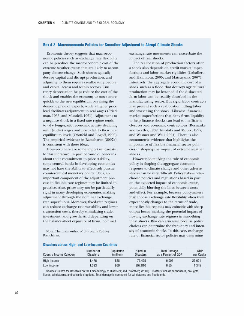
disasters across high- and low-income Countries
Country Income CategoryNumber of Disasters
Population (million)
Killed in Disasters
Total Damage, as a Percent of GDP
GDP per Capita
High income 1,476 828 75,425 0.007 23,021Low income 1,533 869 907,810 0.55 1,345
Sources: Centre for Research on the Epidemiology of Disasters; and Stromberg (2007). Disasters include earthquakes, droughts, floods, windstorms, and volcanic eruptions. Total damage is computed for windstorms and floods only.
Note: The main author of this box is Rodney Ramcharan.

��
specialization patterns and thus the intensity and frequency of terms-of-trade shocks.
Natural disasters can, however, provide cred-ible insight into the impact of economic policy in shaping the aggregate economic response to climate change and other shocks. In particu-lar, disasters are easily observed and yet highly unpredictable. They are also, at least in the short run, not determined by economic choices. Thus, in economics jargon, they can be treated as conditionally exogenous with respect to policy choices. That said, these events do cluster geographically (first and second tables), and the general susceptibility of some countries to natu-ral shocks may influence both economic policy and the response to such shocks. But suscepti-bility is an observable phenomenon that can be included in the estimation framework, reducing the possibility of bias. And even after accounting for geographic clustering, these shocks remain mostly low-probability and unpredictable events for many countries, and therefore are unlikely to be a powerful force in determining economic policy. The Caribbean, for example, is notori-ously hurricane prone, yet an Atlantic hurricane on average has struck one of these islands just seven times in the past �00 years.
The methodology in Ramcharan (�007a) can be used to estimate the role of financial sector policies in shaping the output impact of natural disasters. In the case of floods, for example, let Sit–� denote a variable that takes on the value of zero if there are no floods in country i in year t – � (the previous year) and the ratio of affected land area to the country’s total land
area if a flood does occur. Let Rit denote the Abiad, Detragiache, and Thierry Tressel (�007) de jure financial liberalization index observed in country i on year t. The vector Xit denotes the set of control variables observed for country i in year t.
The estimating equation is
yit = ∑j=�
� [aj Sit–j + ljRit + gj Sit–j *Rit + Xit–jSit–jθj]
+ Xitb + νt + uit,
where the parameters gj test whether the impact of a shock on the outcome variable, yit, depends on the market orientation of the financial system. Because the financial system as well as the shock can affect the equilibrium level of yit, the specifi-
regional differences in disaster incidence and impact
Number of Disasters
Killed per 100,000
Affected per 100,000
Africa 861 2.61 1,453Asia 2,352 0.74 4,303Americas 1,626 0.59 564Europe 863 0.60 206Oceania 324 0.46 2,363
Sources: Centre for Research on the Epidemiology of Disasters; and Stromberg (2007).
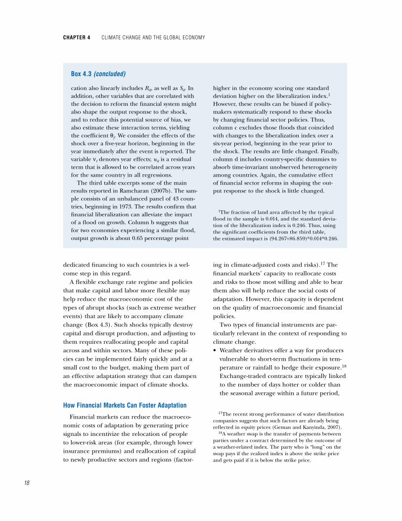
Financial Sector reforms and the impact of Floods on output growth(Dependent variable: real per capita GDP growth)
(a)(b)
Baseline
(c)“ConstantPolicies”
(d)Fixed
Effects
Flood (t – 1) 37.945 70.707 32.146[40.916] [62.509] [51.284]
Index*Flood (t – 1) –7.343 –75.724 –0.244[24.954] [100.034] [27.582]
Flood (t – 2) 13.043 2.490 4.323[35.767] [36.658] [33.569]
Index*Flood (t – 2) 27.832 40.557 30.428[33.379] [32.498] [28.258]
Flood (t – 3) 89.142** 104.159 86.924**[36.503] [102.895] [40.527]
Index*Flood (t – 3) –10.844 –150.389 –13.505[26.197] [169.852] [25.770]
Flood (t – 4) –37.606 –73.439** –39.671*[25.417] [27.862] [23.146]
Index*Flood (t – 4) 86.859** 127.332*** 92.125**[37.567] [35.185] [36.152]
Flood (t – 5) –77.633** –226.517*** –83.121**[35.548] [47.327] [35.773]
Index*Flood (t – 5) 94.267*** 70.670*** 97.687***[14.572] [10.574] [14.122]
Observations 989 842 989R-squared 0.28 0.30 0.37
Source: Ramcharan (2007b). Note: Standard errors, in brackets, are clustered at the
country level. *, **, and *** denote significance at the 10 percent, 5 percent, and 1 percent level, respectively.
how Can Countries best adapt to Climate Change?
Chapter 4 Climate Change and the global eConomy
��
dedicated financing to such countries is a wel-come step in this regard.
A flexible exchange rate regime and policies that make capital and labor more flexible may help reduce the macroeconomic cost of the types of abrupt shocks (such as extreme weather events) that are likely to accompany climate change (Box �.�). Such shocks typically destroy capital and disrupt production, and adjusting to them requires reallocating people and capital across and within sectors. Many of these poli-cies can be implemented fairly quickly and at a small cost to the budget, making them part of an effective adaptation strategy that can dampen the macroeconomic impact of climate shocks.
how Financial markets Can Foster adaptation
Financial markets can reduce the macroeco-nomic costs of adaptation by generating price signals to incentivize the relocation of people to lower-risk areas (for example, through lower insurance premiums) and reallocation of capital to newly productive sectors and regions (factor-
ing in climate-adjusted costs and risks).�7 The financial markets’ capacity to reallocate costs and risks to those most willing and able to bear them also will help reduce the social costs of adaptation. However, this capacity is dependent on the quality of macroeconomic and financial policies.
Two types of financial instruments are par-ticularly relevant in the context of responding to climate change.• Weather derivatives offer a way for producers
vulnerable to short-term fluctuations in tem-perature or rainfall to hedge their exposure.�8 Exchange-traded contracts are typically linked to the number of days hotter or colder than the seasonal average within a future period,
�7The recent strong performance of water distribution companies suggests that such factors are already being reflected in equity prices (Geman and Kanyinda, �007).
�8A weather swap is the transfer of payments between parties under a contract determined by the outcome of a weather-related index. The party who is “long” on the swap pays if the realized index is above the strike price and gets paid if it is below the strike price.
cation also linearly includes Rit, as well as Sit. In addition, other variables that are correlated with the decision to reform the financial system might also shape the output response to the shock, and to reduce this potential source of bias, we also estimate these interaction terms, yielding the coefficient θj. We consider the effects of the shock over a five-year horizon, beginning in the year immediately after the event is reported. The variable νt denotes year effects; uit is a residual term that is allowed to be correlated across years for the same country in all regressions.
The third table excerpts some of the main results reported in Ramcharan (�007b). The sam-ple consists of an unbalanced panel of �� coun-tries, beginning in �97�. The results confirm that financial liberalization can alleviate the impact of a flood on growth. Column b suggests that for two economies experiencing a similar flood, output growth is about 0.�� percentage point
higher in the economy scoring one standard deviation higher on the liberalization index.� However, these results can be biased if policy-makers systematically respond to these shocks by changing financial sector policies. Thus, column c excludes those floods that coincided with changes to the liberalization index over a six-year period, beginning in the year prior to the shock. The results are little changed. Finally, column d includes country-specific dummies to absorb time-invariant unobserved heterogeneity among countries. Again, the cumulative effect of financial sector reforms in shaping the out-put response to the shock is little changed.
�The fraction of land area affected by the typical flood in the sample is 0.0��, and the standard devia-tion of the liberalization index is 0.���. Thus, using the significant coefficients from the third table, the estimated impact is (9�.��7+8�.8�9)*0.0��*0.���.
box 4.3 (concluded)
��
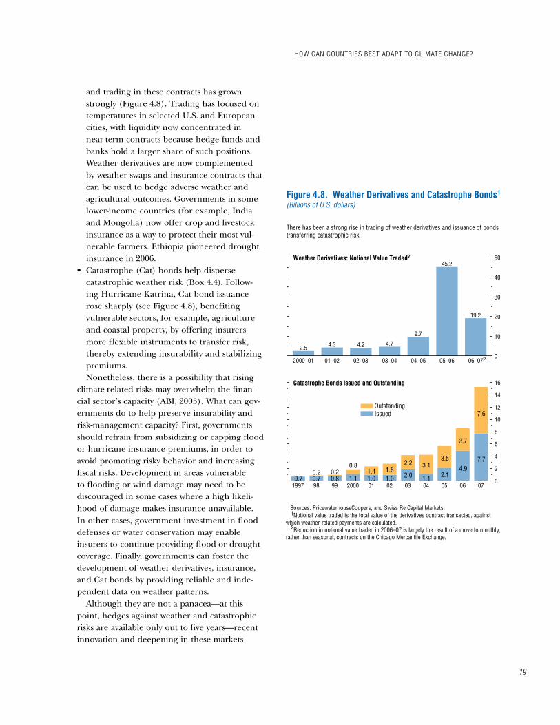
and trading in these contracts has grown strongly (Figure �.8). Trading has focused on temperatures in selected U.S. and European cities, with liquidity now concentrated in near-term contracts because hedge funds and banks hold a larger share of such positions. Weather derivatives are now complemented by weather swaps and insurance contracts that can be used to hedge adverse weather and agricultural outcomes. Governments in some lower-income countries (for example, India and Mongolia) now offer crop and livestock insurance as a way to protect their most vul-nerable farmers. Ethiopia pioneered drought insurance in �00�.
• Catastrophe (Cat) bonds help disperse catastrophic weather risk (Box �.�). Follow-ing Hurricane Katrina, Cat bond issuance rose sharply (see Figure �.8), benefiting vulnerable sectors, for example, agriculture and coastal property, by offering insurers more flexible instruments to transfer risk, thereby extending insurability and stabilizing premiums.Nonetheless, there is a possibility that rising
climate-related risks may overwhelm the finan-cial sector’s capacity (ABI, �00�). What can gov-ernments do to help preserve insurability and risk-management capacity? First, governments should refrain from subsidizing or capping flood or hurricane insurance premiums, in order to avoid promoting risky behavior and increasing fiscal risks. Development in areas vulnerable to flooding or wind damage may need to be discouraged in some cases where a high likeli-hood of damage makes insurance unavailable. In other cases, government investment in flood defenses or water conservation may enable insurers to continue providing flood or drought coverage. Finally, governments can foster the development of weather derivatives, insurance, and Cat bonds by providing reliable and inde-pendent data on weather patterns.
Although they are not a panacea—at this point, hedges against weather and catastrophic risks are available only out to five years—recent innovation and deepening in these markets
2000–01 01–02 02–03 03–04 04–05 05–06 06–070
10
20
30
40
50
2.5 4.3 4.2 4.7
9.7
45.2
19.2
Figure 4.8. Weather Derivatives and Catastrophe Bonds(Billions of U.S. dollars)
There has been a strong rise in trading of weather derivatives and issuance of bondstransferring catastrophic risk.
Sources: PricewaterhouseCoopers; and Swiss Re Capital Markets. Notional value traded is the total value of the derivatives contract transacted, against which weather-related payments are calculated. Reduction in notional value traded in 2006–07 is largely the result of a move to monthly, rather than seasonal, contracts on the Chicago Mercantile Exchange.
Weather Derivatives: Notional Value Traded2
1997 98 99 2000 01 02 03 04 05 06 070
2
4
6
8
10
12
14
16
0.7 0.7 0.8 1.1 1.0 1.0 2.0 1.1 2.14.9
7.7
0.2 0.20.8
1.4 1.82.2 3.1
3.5
3.7
7.6OutstandingIssued
Catastrophe Bonds Issued and Outstanding
2
1
1
2
how Can Countries best adapt to Climate Change?
Chapter 4 Climate Change and the global eConomy
�0
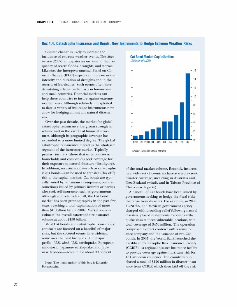
Climate change is likely to increase the incidence of extreme weather events. The Stern Review (�007) anticipates an increase in the fre-quency of severe floods, droughts, and storms. Likewise, the Intergovernmental Panel on Cli-mate Change (IPCC) expects an increase in the intensity and duration of droughts and in the severity of hurricanes. Such events often have devastating effects, particularly in low-income and small countries. Financial markets can help these countries to insure against extreme weather risks. Although relatively unexploited to date, a variety of insurance instruments now allow for hedging almost any natural disaster risk.
Over the past decade, the market for global catastrophe reinsurance has grown strongly in volume and in the variety of financial struc-tures, although its geographic coverage has expanded to a more limited degree. The global catastrophe reinsurance market is the wholesale segment of the insurance market. Typically, primary insurers (those that write policies to households and companies) seek coverage for their exposure to natural disasters (first figure). In addition, securitizations—such as catastrophe (Cat) bonds—can be used to transfer (“lay off”) risk to the capital markets. Cat bonds are typi-cally issued by reinsurance companies, but are sometimes issued by primary insurers or parties who seek self-insurance, such as governments. Although still relatively small, the Cat bond market has been growing rapidly in the past few years, reaching a total capitalization of more than $�� billion by end-�007. Market sources estimate the overall catastrophe reinsurance volume at about $��0 billion.
Most Cat bonds and catastrophe reinsurance contracts are focused on a handful of major risks, but the covered events have widened some over the past two years. The major perils—U.S. wind, U.S. earthquake, European windstorm, Japanese earthquake, and Japa-nese typhoon—account for about 90 percent
of the total market volume. Recently, insurers in a wider set of countries have started to seek disaster coverage, including in Australia and New Zealand (wind), and in Taiwan Province of China (earthquake).
A handful of Cat bonds have been issued by governments seeking to hedge the fiscal risks that arise from disasters. For example, in �00�, FONDEN, the Mexican government agency charged with providing relief following natural disasters, placed instruments to cover earth-quake risks at three vulnerable locations, with total coverage of $��0 million. The operation comprised a direct contract with a reinsur-ance company and the issuance of two Cat bonds. In �007, the World Bank launched the Caribbean Catastrophe Risk Insurance Facility (CCRIF)—a regional disaster insurance facility to provide coverage against hurricane risk for �� Caribbean countries. The countries pur-chased a total of $��0 million in disaster insur-ance from CCRIF, which then laid off the risk
box 4.4. Catastrophe insurance and bonds: new instruments to hedge extreme Weather risks
Note: The main author of this box is Eduardo Borensztein.
1998 99 2000 01 02 03 04 05 06 070
2
4
6
8
10
12
14
16
Cat Bond Market Capitalization(Billions of USD)
Source: Swiss Re Capital Markets.
Box 4.4 Figure 1

��
through reinsurers and capital markets. Scale is a significant advantage of pooling multicoun-try risk. The minimum economically feasible size for a Cat bond is estimated to be about $�00 million.
Market instruments typically do not provide full insurance coverage for macro risks. The stan-dard contract or Cat bond, including those used by FONDEN and CCRIF, applies a “parametric” trigger—the insurance payment is triggered by the occurrence of a natural event of a certain magnitude, rather than by a calculation of the losses suffered. The trigger can be a particular wind speed or a certain intensity and/or depth of an earthquake measured at a specified location. The parametric trigger simplifies enormously the monitoring and execution of the insurance contract and permits immediate payment upon the occurrence of the covered disaster.� The event can be monitored by a third party, such as the U.S. National Hurricane Center.
Parametric insurance, however, can leave a fair amount of residual risk uncovered (“basis risk” in insurance language). A natural phenom-enon may cause considerable damage without crossing the parametric boundary. Indeed, Hur-ricane Dean, which caused significant damage in Belize and Jamaica in August �007, did not trigger any payments under the CCRIF because winds did not reach the required speeds at the specified locations. As with any other insurance structure, there is a trade-off between cost and coverage in parametric insurance. Basis risk can be reduced but only at a higher cost, and the insured must choose their preferred trade-off between risk and cost.
Pricing in the Cat market has been punctu-ated by the impact of large disasters—par-ticularly U.S. hurricanes Andrew in �99� and Katrina in �00� (second figure). There has also been an upward trend in insurance premi-
�A more common feature of standard reinsurance contracts is an “indemnity” trigger—namely, the dam-age suffered by the insured. There are also intermedi-ate options such as modeled losses and indices based on a parametric occurrence.
ums, in part related to upward reassessments of disaster risk. The reason for the premium spikes is that, after a large disaster, reinsurance companies need to rebuild capital in order to preserve their solvency and credit ratings. This may be a long process if capital markets are not fluid, and in the meantime insurance premiums remain elevated. Yet the figure also suggests that the post-Katrina rise, although broadly com-mensurate with the post-Andrew increase, was fairly short lived. The reversal of the premium increase took place despite both a tightening of standards by credit rating agencies and an upward reassessment of disaster risk by weather modeling firms and market participants. Part of the reason for the quick reversal was the rapid entry of new investors such as hedge funds, banks, and private equity investors, who sup-plied additional capital through various market structures. In addition to Cat bonds, new mar-ket instruments include bank loans and equity, especially in the form of “sidecars”—legally
1985 87 89 91 93 95 97 99 2001 03 05 07:Q10
20
40
60
80
100
120
140
160
180
200
Detrended Catastrophe Insurance Premiums(Index, 1985 = 100)
Source: IMF staff calculations based on Lane Financial, LLC.
Box 4.4 Figure 2
Andrew
Post 9/11
Katrina
how Can Countries best adapt to Climate Change?

Chapter 4 Climate Change and the global eConomy
��
separate, special-purpose reinsurance compa-nies that raise short-term capital through private equity and debt.
An Unexploited Opportunity?
Low-income and small countries are espe-cially vulnerable to natural disasters because of more limited geographical diversification, higher percentages of the population living in exposed areas, and higher dependence on natural rainfall and benign weather conditions for agricultural production. According to the World Health Organization’s Emergency Events Database, two hurricanes that hit Belize in �000 and �00� each caused damage equivalent to more than �0 percent of GDP and impaired public debt sustainability (Borensztein, Cavallo, and Valenzuela, �008).� Even less-extreme events can involve enormous indirect costs. Drought has been linked to higher incidence of armed conflict in low-income countries, essen-tially through its effect on economic growth and poverty (Miguel, Satyanath, and Sergenti, �00�).
Faced with such catastrophic risk, low-income countries tend to rely on foreign aid or some form of self-insurance (Borensztein, Cavallo, and Valenzuela, �008). Aid flows, however, are unreliable, may arrive late, and seem somewhat dependent on the extent to which the media covers the disaster. Self-insurance strategies include borrowing when a disaster occurs or accumulating resources in a dedicated fund. But there is a critical difference between insurance and self-insurance. If a country purchases insur-ance (say by issuing a Cat bond), it will receive ensured payment in a disaster that offsets the loss suffered, albeit imperfectly. By resorting to borrowing, by contrast, the country can spread over time the cost of the disaster but still bears the full economic loss. Moreover, self-insur-ance strategies may have other problems. For example, self-insurance funds may be appropri-ated for other uses when they become sizable. There is, in fact, an optimal combination of
�Cost estimates should be viewed with appropriate caution and are subject to significant revisions.
insurance and borrowing (or self-insurance), which depends on many factors, including the size of the potential loss, the cost of insurance, interest rates, ease of access to external financ-ing, and the extent to which credit rating agen-cies incorporate market insurance coverage in their evaluation.
Despite their advantages, few countries have issued Cat bonds or sought disaster insurance. One reason may be cost. Cat premiums can be high owing to various factors, including the required technical studies by modeling agen-cies, legal costs, and remuneration of the capital requirements for insurance and reinsurance companies under imperfect market conditions (see Froot, �00�). (To some extent, however, the cost of insurance for emerging and develop-ing economies is tempered by the diversification value of these perils within the global financial market.) Another reason may be policymak-ers’ fears of engaging in unusual and complex operations, which they may not fully under-stand. Politicians also tend to focus on the near term and hence are not motivated to spend money on insurance that may mainly benefit their successors in office.
Catastrophe insurance instruments also can be useful for international financial institu-tions that seek to provide broad support for such insurance programs, as in the case of CCRIF. The World Bank has other projects under way to provide insurance to farmers in various countries, including India and Mon-golia, and it is hedging these risks in global markets. Disaster insurance is a means for aid agencies to deal with the budget limitations that can arise in years when they must respond to several large disasters. In this regard, the United Nations’ World Food Program (WFP), in collaboration with the World Bank, ran a pilot program for drought insurance in Ethio-pia in �00�, which offered coverage to farmers who could be affected by insufficient rainfall. The WFP laid off the risk in the global reinsur-ance market. In the event, no payments were triggered because rains were adequate in all the covered areas.
box 4.4 (concluded)
��
holds the promise that they have considerable potential to promote adaptation to climate change. The growth of hedge funds and the strong appetite for risks that are uncorrelated with other financial markets should ensure con-tinuing demand for financial instruments that pay investors a premium for taking weather risk even in the face of climate change (van Lennep and others, �00�; and Bonaccolta, �007).
All in all, countries’ adaptive capacity is likely to increase in the future, as incomes rise, technologies emerge, financial markets develop, and understanding of climate change improves. Nonetheless, at high degrees of warming, the limitations of adaptation are likely to be reached relatively quickly. Together with the rising prob-ability of catastrophic risk, this points to a need for mitigation.
how Can Countries effectively and efficiently mitigate Climate Change?
A successful policy framework for mitigating climate change must satisfy several criteria.• To be effective, mitigation policy must raise
the prices of GHGs to reflect the marginal social damage from emissions. Higher GHG prices would help generate incentives for reducing production and consumption of emission-intensive goods and for develop-ment and adoption of new, low-emission technologies.
• Mitigation policy must be applied across all GHGs, firms, countries, sectors, and time peri-ods in order to ensure that policy achieves the desired objectives at the lowest possible cost.
• It is important to address distributional con-siderations across firms, income groups, and generations, both for reasons of fairness and distributional justice as well as to ensure that policies remain politically viable.
• Mitigation policies must be flexible and robust to changing economic conditions and to new scientific information about climate change, because highly volatile outcomes could increase the economic costs of policies and reduce political support.
• Mitigation policies must be enforceable and have “dynamic consistency,” meaning that governments have incentives to keep them in place, in order to induce the needed behav-ioral response.Many policy instruments have been con-
sidered for reducing emissions. The most prominent have been emission taxes, tradable emission permits, performance standards, incentives for the adoption of energy-saving technologies, and subsidies for the reduction of emissions or introduction of clean technolo-gies (Box �.�).�9 Market-based policies, such as emission taxes (often called carbon taxes�0) and permit-trading programs, have an impor-tant advantage over performance standards in that they create a common price for emissions. Common pricing encourages emissions to be concentrated in firms that can produce more efficiently.
The choice between carbon taxes and cap-and-trade systems is less clear cut. Carbon taxes have an important advantage over cap-and-trade systems in that they result in a stable price for emissions (cap-and-trade policies seek to stabi-lize the quantity of emissions, but allow prices to fluctuate). Stable prices for emissions are critical for firms making long-term decisions about investment and innovation in low-emission tech-nologies. Carbon taxes also provide for greater flexibility in the face of changing economic conditions, allowing firms to reduce emissions more during periods of slow demand growth and less during periods of high demand growth, when the cost of doing so would be higher. In contrast, cap-and-trade systems could give rise to volatile emission pricing when demand conditions change. Carbon taxes also generate revenues that can be used to enhance efficiency
�9Performance standards include, for example, limits on emissions per kilowatt hour of electricity and fuel-economy requirements on vehicles.
�0Taxing the carbon content of emissions is equivalent to taxing carbon dioxide. Carbon dioxide accounts for the largest share of emissions. Emissions of other GHGs (methane, nitrous oxide, and fluorinated gases) are often expressed in terms of their carbon dioxide equivalents.
how Can Countries effeCtively and effiCiently mitigate Climate Change?
Chapter 4 Climate Change and the global eConomy
��
Under Annex I of the Kyoto Protocol, signatory countries� agree to reduce their greenhouse gas (GHG) emissions by 8 per-cent relative to �990 levels by �008–��. This is the principal international policy framework providing incentives to mitigate the impact of global warming. The main implementation mechanism for the Kyoto Protocol in Europe is the European Union Emissions Trading Scheme (EU-ETS). Two additional compliance vehicles, the Clean Development Mechanism (CDM) and Joint Implementation, enable Annex I countries to gain credits for emission reductions arising from investments made in countries not subject to binding targets.
The EU-ETS is an international cap-and-trade system, projected to reduce emissions by �.� percent compared to a business-as-usual scenario by �0�0,� although it needs further reform in order to realize its full potential for large-scale, efficient mitigation. During Phases I (�00�–07) and II (�008–��), carbon dioxide (CO�) emission rights were allocated to about ��,000 energy-intensive installations across the European Union (mostly electric power utilities and major industrial emitters), representing about �0 percent of total EU carbon emissions. The volume of trading in the market was about �.� billion tons of CO� in �007 and was valued at about €�8 billion (up �� percent over �00� val-ues).� Intended to minimize abatement costs for a given emission target, the system is subject to a number of design flaws, which have reduced its effectiveness. First, excess quotas and market uncertainty have caused permit prices to be too low and volatile. In fact, prices fell to zero in the second half of �007 (although prices are generally higher under Phase II). Second, the high share of free allocations (at least 9� per-
Note: The main authors of this box are Ben Jones and Jon Strand, with input from Paul Mills.
�A group of industrialized nations including east-ern Europe, the OECD, Russia, and the United States (although the latter did not ratify the treaty).
�See Capoor and Ambrosi (�007).�See Point Carbon Research (�008).
cent in Phase I and 90 percent in Phase II) led to windfall profits and forgone public revenues and reduced abatement incentives by creating expectations of future free allocations based on current emissions.� These problems were exac-erbated by rules under which exiting firms lose their free allocations while new firms typically receive free allocations.� Third, the carbon price is poorly coordinated with policies, taxes, and regulations implemented in markets outside the scope of the scheme, such as heating and trans-portation. Efforts to limit the extent of some of these (and other) problems are under way, for example, by expanding the system to include new industries (including, for example, aviation within the European Union) and new gases; preannouncing future constraints (starting with an �� percent reduction in Phase III against the previous commitment framework); moving to full auctioning of permits (starting with at least �0 percent in �0��); and harmonizing the rules for cap-setting and entry and exit.
The CDM enables Annex I countries to gain credits for investment in less-carbon-intensive technologies in developing and emerging market economies (currently not subject to mitigation targets), facilitating access to lower-cost abatement opportunities and helping to promote development by adding to the capital stock in these economies. The CDM market has grown rapidly in recent years, with primary markets estimated at 9�0 million tons of CO� and valued at approximately €�� billion in �007 (up almost �00 percent over �00� values). Sev-eral issues, however, warrant attention. First, the capacity to monitor and verify the “additional-ity” of emission reductions, formally a condition for CDM project approval, is often unclear. Although emissions may be reduced through a
�See Böhringer and Lange (�00�) and Rosendahl (�00�) for discussion. Rosendahl points out that when future quotas are updated to reflect current emis-sions, the quota price could be several times the level of marginal emission abatement cost, indicating that very little abatement is taking place.
�See, for example, Åhman and Holmgren (�00�); and Åhman, Burtraw, Kruger, and Zetterberg (�007).
box 4.5. recent emission-reduction policy initiatives
��
particular CDM project, it is difficult to quantify overall emission reductions in economies that are not subject to overarching emission con-straints or policies (such counterfactuals are in some sense impossible to ascertain, even given elaborate case-by-case administrative proce-dures). Second, given the high degree of policy risk after �0��, virtually no abatement has been achieved for projects subject to long invest-ment-return periods, such as in energy supply markets—most investment has targeted emis-sion reductions from industrial processes. Third, forgone deforestation has so far been left out of the CDM, and its inclusion will require over-coming complex administrative and governance problems, especially in relation to establishing a baseline, monitoring and enforcing compli-ance, and managing “leakage” risks. Finally, few CDM projects have yet been carried out in the poorest countries (with Brazil, China, and India so far dominating), which raises distributional concerns.
In addition, many countries, including non-signatories to the Kyoto Protocol (such as the United States) and major developing economies that are not subject to binding targets under the agreement, have implemented domestic policies that reduce emissions. (The table summarizes these policies for a selected group of countries.) These policies are typically motivated less by cli-mate change concerns than by other consider-ations, for example, productivity improvements, energy security, and the abatement of local pollution. However, other domestic policies, such as energy subsidies, may have opposing effects, leading to strong overall growth in emis-sions, particularly from expansion of fossil-fuel-based energy supply in developing economies. Although domestic efforts are welcome—indeed essential—thus far they have provided weak and often poorly coordinated incentives and have also lacked transparency. These factors have impeded effective and efficient international coordination of mitigation efforts. Two primary types of such domestic emission-reduction poli-cies are performance standards and technology subsidies.
Performance standards, though often less attractive than market mechanisms, have resulted in substantial emission reductions in markets for vehicles, buildings, and appliances, for which emissions are diffuse, transaction costs from compliance with market incentives are high, and the credibility of carbon markets is still being established. In road transport, Japan’s Top Runner program (see table) has yielded significant energy savings, estimated at �� per-cent during �99�–�00� in the case of diesel passenger vehicles (Energy Conservation Centre Japan, �00�). In the United States, Corporate Average Fuel Economy (CAFE) standards, while less demanding than European or Japanese standards, have improved vehicle efficiency since their introduction in �97�. However, laxer restrictions on sport-utility vehicles and small trucks have constrained their overall effec-tiveness when consumer preferences shifted toward heavier vehicle classes. Regulatory codes applied to buildings, for example in Califor-nia, are estimated to have saved approximately �0,000 gigawatt hours (GWh) of electricity annually, about � percent of total electricity use in �00� (California Energy Commission, �00�). More stringent commitments to improve the energy efficiency of U.S. federal buildings were announced in December �007. U.S. standards on appliances are projected to reduce annual residential emissions by about �7 metric tons of CO� (MtCO�) by �0�0, roughly 9 percent of household emissions (Meyers and others, �00�).
Technology subsidies (including tax incen-tives) have been widely used to support renew-able electricity and biofuel production, but they are not a cost-effective substitute for proper carbon pricing. Even so, they may be an appropriate response to failures in technology markets. Support typically aims to reduce the cost of research and development and capital investment, or to guarantee higher end-user prices. In Germany, for example, a renewable electricity “feed-in” tariff system is expected to impose additional costs of €�0 billion–€�� bil-lion on consumers between �000 and �0�� at a cost of approximately €0.�0 a kilowatt hour
how Can Countries effeCtively and effiCiently mitigate Climate Change?
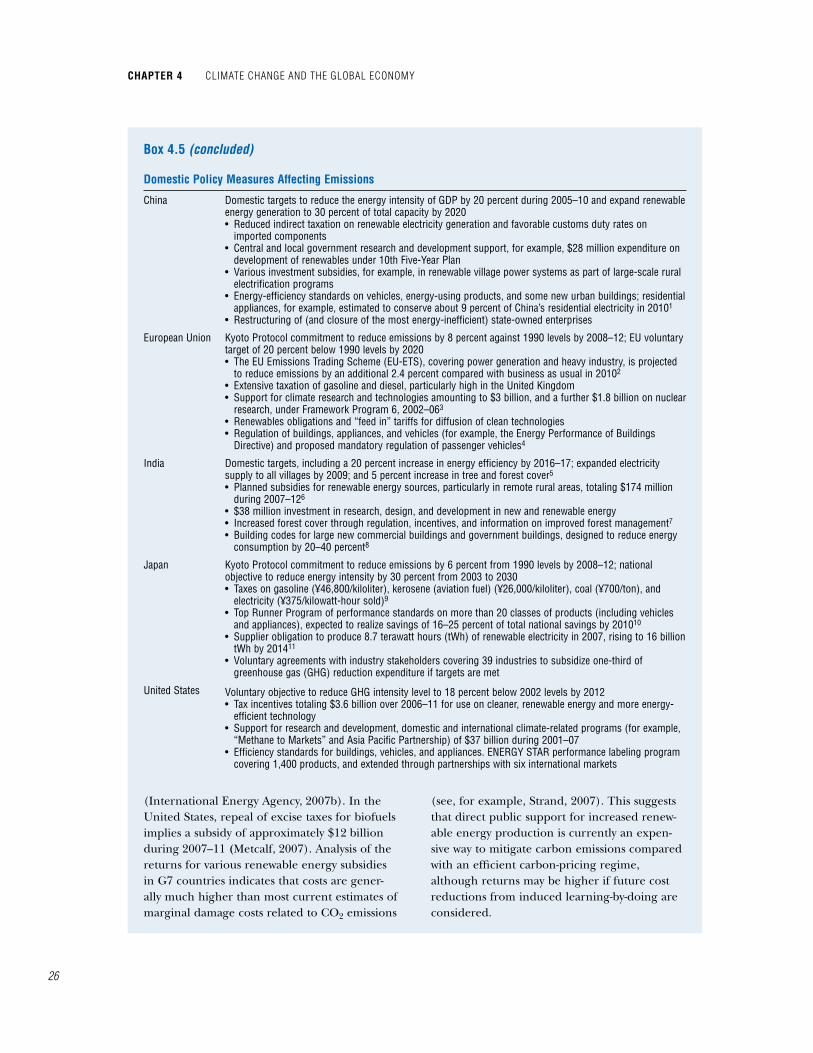
Chapter 4 Climate Change and the global eConomy
��
(International Energy Agency, �007b). In the United States, repeal of excise taxes for biofuels implies a subsidy of approximately $�� billion during �007–�� (Metcalf, �007). Analysis of the returns for various renewable energy subsidies in G7 countries indicates that costs are gener-ally much higher than most current estimates of marginal damage costs related to CO� emissions
(see, for example, Strand, �007). This suggests that direct public support for increased renew-able energy production is currently an expen-sive way to mitigate carbon emissions compared with an efficient carbon-pricing regime, although returns may be higher if future cost reductions from induced learning-by-doing are considered.
box 4.5 (concluded)
domestic policy measures affecting emissions
China Domestic targets to reduce the energy intensity of GDP by 20 percent during 2005–10 and expand renewable energy generation to 30 percent of total capacity by 2020• Reduced indirect taxation on renewable electricity generation and favorable customs duty rates on
imported components• Central and local government research and development support, for example, $28 million expenditure on
development of renewables under 10th Five-Year Plan • Various investment subsidies, for example, in renewable village power systems as part of large-scale rural
electrification programs• Energy-efficiency standards on vehicles, energy-using products, and some new urban buildings; residential
appliances, for example, estimated to conserve about 9 percent of China’s residential electricity in 20101
• Restructuring of (and closure of the most energy-inefficient) state-owned enterprises
European Union Kyoto Protocol commitment to reduce emissions by 8 percent against 1990 levels by 2008–12; EU voluntary target of 20 percent below 1990 levels by 2020• The EU Emissions Trading Scheme (EU-ETS), covering power generation and heavy industry, is projected
to reduce emissions by an additional 2.4 percent compared with business as usual in 20102
• Extensive taxation of gasoline and diesel, particularly high in the United Kingdom• Support for climate research and technologies amounting to $3 billion, and a further $1.8 billion on nuclear
research, under Framework Program 6, 2002–063
• Renewables obligations and “feed in” tariffs for diffusion of clean technologies• Regulation of buildings, appliances, and vehicles (for example, the Energy Performance of Buildings
Directive) and proposed mandatory regulation of passenger vehicles4
India Domestic targets, including a 20 percent increase in energy efficiency by 2016–17; expanded electricity supply to all villages by 2009; and 5 percent increase in tree and forest cover5
• Planned subsidies for renewable energy sources, particularly in remote rural areas, totaling $174 million during 2007–126
• $38 million investment in research, design, and development in new and renewable energy• Increased forest cover through regulation, incentives, and information on improved forest management7• Building codes for large new commercial buildings and government buildings, designed to reduce energy
consumption by 20–40 percent8
Japan Kyoto Protocol commitment to reduce emissions by 6 percent from 1990 levels by 2008–12; national objective to reduce energy intensity by 30 percent from 2003 to 2030 • Taxes on gasoline (¥46,800/kiloliter), kerosene (aviation fuel) (¥26,000/kiloliter), coal (¥700/ton), and
electricity (¥375/kilowatt-hour sold)9
• Top Runner Program of performance standards on more than 20 classes of products (including vehicles and appliances), expected to realize savings of 16–25 percent of total national savings by 201010
• Supplier obligation to produce 8.7 terawatt hours (tWh) of renewable electricity in 2007, rising to 16 billion tWh by 201411
• Voluntary agreements with industry stakeholders covering 39 industries to subsidize one-third of greenhouse gas (GHG) reduction expenditure if targets are met
United States Voluntary objective to reduce GHG intensity level to 18 percent below 2002 levels by 2012• Tax incentives totaling $3.6 billion over 2006–11 for use on cleaner, renewable energy and more energy-
efficient technology• Support for research and development, domestic and international climate-related programs (for example,
“Methane to Markets” and Asia Pacific Partnership) of $37 billion during 2001–07• Efficiency standards for buildings, vehicles, and appliances. ENERGY STAR performance labeling program
covering 1,400 products, and extended through partnerships with six international markets

��
(by lowering other taxes) or equity (by com-pensating groups disadvantaged by the policy). However, under carbon taxes, the quantity of emission reductions is uncertain. Taxes also may be politically difficult to implement.
There are ways to reduce the disadvantages of cap-and-trade systems. Price volatility, for example, can be reduced by introducing safety valves that allow governments to sell some temporary permits if permit prices exceed some prespecified “trigger” levels, by allow-ing the depositing and borrowing of permits, or by creating a central-bank-type institution for overseeing permit markets. Such hybrid policies—combining elements of a carbon tax and a permit-trading system—could be superior to the respective single policy instru-ments (Pizer, �00�). Raising the trigger price of the safety valve over time would allow for the simultaneous targeting of emission prices, over the short run, and their quantity, over the long
run.�� See Box �.� for a further discussion of these and other issues that arise in the context of mitigation policies.��
macroeconomic effects of international mitigation policies
The importance of cross-border linkages is assessed by examining the macroeconomic effects of alternative mitigation policies using a dynamic intertemporal global general equi-librium model (the �007 version of G-Cubed, developed by McKibbin and Wilcoxen, �998). G-Cubed is well suited for evaluating the short-, medium-, and long-term effects of mitigation
��See Aldy and Stavins (�007) for a discussion of alternative mitigation policy proposals, including hybrid schemes proposed by Kopp, Morgenstern, and Pizer (�997) and McKibbin and Wilcoxen (�997, �00�b, �00�c).
��See also the October �007 World Economic Outlook.
Brazil National objective to increase the share of renewable energy sources to 10 percent by 2030 and expand availability of electricity to an additional 12 million citizens• Roughly 50 percent reduction in deforestation between 2004 and 2006 through improved satellite
monitoring, land use controls, and sustainable logging incentives• Mandatory 22 percent blend of ethanol in gasoline and 2 percent mix of biosourced diesel (rising to 5
percent in 2013)• Subsidized lines of credit for biodiesel production; support for research into biodiesel and expansion of
ethanol and sugar program to other products• 20-year feed-in tariffs for renewable electricity generators;12 supplier obligation to invest 1 percent of net
operational income in efficiency measures and research and development• Adoption of U.S. efficiency standards for light vehicles and EU standards for motorcycles and heavy
vehicles• Investment in decentralized, renewable electricity as part of “Light for All” electrification program
1China Markets Group, Lawrence Berkeley Laboratories: http://china.lbl.gov/china_buildings-asl-standards.html.2See Capoor and Ambrosi (2007).3EU action against climate change: research and development to stimulate climate-friendly technologies.4The Energy Performance of Buildings Directive is designed to realize an estimated cost-effective savings potential of about 22 percent
of present consumption in buildings across the European Union by 2010. The European Commission is proposing to reduce the average emissions of CO2 from new passenger cars in the European Union from about 160 grams a kilometer to 130 grams a kilometer in 2012.
5India, Planning Commission (2007).6India, Ministry of New and Renewable Energy (2006).7India, Ministry of Environment and Forests (2006), p. 25.8India, Ministry of Environment and Forests and Ministry of Power Bureau of Energy Efficiency (2007), p. 7.9Japan (2006).10Nordqvist (2006), p. 6.11“Outline of the Renewable Portfolio Standard (RPS) System.” www.rps.go.jp/RPS/new-contents/english/outline.html.12Brazil (2007), pp. 22, 27.
domestic policy measures affecting emissions (concluded)
how Can Countries effeCtively and effiCiently mitigate Climate Change?
Chapter 4 Climate Change and the global eConomy
��
This box highlights some broader issues in the design of domestic emission-mitigation policies, beyond the basic choice between an emission tax and a cap-and-trade system (see Kopp and Pizer, �007, for an in-depth discussion of design issues).
Building Flexibility into Emission-Control Policies
A major concern with rigid annual emission caps is the risk of volatility in emission prices that might be caused, for example, by changes in demand conditions or disruptions in energy markets. Severe volatility in allowance prices may deter investments in emission-saving tech-nologies that have large upfront costs and could undermine political support for a cap-and-trade system. However, there are ways to partly address this problem.
One option is to include a safety-valve mecha-nism, under which permit prices are prevented from exceeding a certain ceiling price, with the regulator authorized to sell whatever addi-tional allowances must be introduced into the market to prevent prices rising beyond this level (Pizer, �00�). Another option is to allow firms to borrow permits from the government during periods of high permit prices and to deposit such permits when there is downward price pressure, to help smooth out sharp price fluctu-ations. The European Union Emissions Trading Scheme (EU-ETS) now allows for permit bank-ing (though not borrowing). A further option is government oversight of carbon markets through a new body, much like a central bank, which would intervene to sell or buy permits in response to unexpectedly high or low permit prices. Again, this type of oversight could help to stabilize the permit market while also provid-ing greater confidence in the achievement of longer-run emission goals.
Yet some flexibility in permit prices actu-ally may be beneficial, as this enables future knowledge about the likely impact of global warming to be reflected in real-time permit prices and abatement decisions. For example,
when deciding whether there is a need for intervention, a “climate central bank” could take into account the factors driving changes in emission prices and allow permanent shocks to be reflected in prices. Even without the climate central bank, under a cap-and-trade regime that allowed depositing and borrow-ing of permits, if new evidence emerges that warming is occurring faster than projected, speculators would anticipate a tightening of the future emission cap, which would instantly shift up the trajectory of current and expected future permit prices (before any adjustment to the cap). In contrast, it may take some time to enact a legislative change in emission tax rates to reflect new scientific information, leaving emission control suboptimal during the period of policy stickiness.
Using Revenues to Keep Policy Costs Down
How the government uses the revenues from carbon taxes or cap-and-trade systems, to the extent that allowances are auctioned, can have a substantial effect on the overall costs of the policy. For example, if revenues are used to lower personal income taxes, this reduces the disincentive effects of these broader taxes on work effort and savings, offsetting the negative effect of higher energy prices on economic activity. Policies that do not exploit the revenue-recycling benefit are more costly, namely, cap-and-trade systems with free allowance allocation or emission taxes and cap-and-trade policies with auctioned allowances, where revenues are not used productively. For example, Parry, Williams, and Goulder (�999) estimate that the overall costs of moderately scaled emission per-mit systems with free allocation are more than double those for the equivalent, revenue-neutral carbon tax for the United States.
Compensating Low-Income Households and Energy-Intensive Firms
Fairness is a major issue for emission-mitiga-tion policies because low-income households spend a relatively high share of their budgets on energy-intensive goods such as electricity, home
box 4.6. Complexities in designing domestic mitigation policies
Note: The main author of this box is Ian Parry.
��
heating fuels, and gasoline, and are therefore more vulnerable to increases in the price of these goods. Cap-and-trade systems with free permit allocation provide no mechanism for addressing these concerns. But if allowances are auctioned, or emission taxes are implemented, fairness concerns may be addressed by recycling some of the revenue in ways that particularly benefit low-income households, such as reduc-tions in payroll taxes or increases in income tax thresholds (Metcalf, �007; and Dinan and Rog-ers, �00�). Some elderly or other nonworking households may require compensation through other means, such as targeted energy-assistance programs.
On the other hand, free allowance alloca-tions can provide compensation for (politically influential) industries adversely affected by climate policy, which helps to reduce opposi-tion from vested interests. However, according to Bovenberg and Goulder (�00�), only a small fraction of allowances must be given away for free to provide such compensation, and so most allowances could still be auctioned. Ideally, any compensation would be progressively phased out over time. This would avoid practical dif-ficulties in updating free allowance allocations as firms grow at different rates over time and would increase the potential fiscal dividend. In fact, after power companies reaped large windfall profits from the allowance giveaway in the initial phase of the EU-ETS, the plan is now to transition to �00 percent allowance auctions by �0�0. Transitory compensation for affected industries also could be provided under an emission tax, for example, by applying the tax only to emissions in excess of some threshold level or by providing temporary corporate tax relief for energy-intensive firms downstream of the formal emission tax regime.
Advantages of an Upstream Program
Ideally, a carbon tax or emission trading system would be applied upstream in the fossil fuel supply chain (on petroleum refiners, coal producers, etc.), because this would encompass all possible sources of emissions when fuels are
later combusted. Fuel producers would pay a tax, or be required to hold permits, in propor-tion to a fuel’s carbon content, and therefore emission taxes or permit prices would be passed forward into fossil fuel prices and ultimately into the price of electricity and other energy-intensive products. This would provide incen-tives for emission-reducing behavior throughout the economy. Downstream trading programs, like the EU-ETS, currently cover electricity and large industrial emitters, which account for only about one-half of total CO� emissions (Kopp and Pizer, �007). Therefore, they preclude many low-cost abatement opportunities, for example in the transportation sector. Upstream programs are also easier to administer. In the European Union or the United States, they would involve regulation of only about �,000–�,000 entities, compared with ��,000 entities or more in a downstream program.
Incorporating All Sources of GHGs and Options for Sequestration
Insofar as possible, it is important to include non-CO� greenhouse gases (GHGs) into any emission-mitigation program. In the United States these gases currently account for about �0 percent of total GHGs when gases are expressed on an equivalent basis for warming potential over their atmospheric lifespan, whereas at the global level these gases account for about one-third of total GHGs (US CCSP, �007). Some of these gases (such as vented methane from underground coal mines and fluorinated gases used as refrigerants and in air conditioners) are fairly straightforward to monitor and incorporate through permit-trading ratios or emission taxes, reflecting their relative global warming potential. Methane and nitrous oxides from landfills, manure manage-ment, and soil management might be incor-porated into an emission-offset program. In that case, the onus would be on the individual entity to demonstrate valid emission reductions for crediting. However the remaining emission sources, which account for about a third of non-CO� GHGs in the United States, are especially
how Can Countries effeCtively and effiCiently mitigate Climate Change?
Chapter 4 Climate Change and the global eConomy
�0
difficult to monitor (for example, methane from ruminants).
Although still in the developmental stage, a potentially important means of reducing emissions from coal plants could be emission capture and storage underground (for example, in depleted oil reservoirs). Incentives for adopt-ing this sequestration technology could be provided through emission offsets or tax credit provisions, although, according to Deutsch and Moniz (�007), the price of carbon would need to be higher than about $�� a ton to make the technology commercially viable. At least for the short term, facilities should be charged for any emission seepage from the underground sink. Because the incorporation and operation of carbon-capture technologies would be fairly easy to verify, emission sources in advanced econo-mies might fund such investments in emerging economies to offset some of their own mitiga-tion obligations.
Biological sequestration could also be a potentially cost-effective way to reduce emis-sions (Stavins and Richards, �00�). Ideally, farms that increased forestland coverage would be credited, and those that shifted from forests to agriculture would be penalized. For the United States, it would be feasible to incorpo-rate forestry into a national emission-mitiga-tion program, given that transitions between forest and agricultural land in the absence of any carbon policy are relatively small (Sedjo and Toman, �00�). Land use changes might be monitored through remote sensing from satellites or aircraft, with the carbon implica-tions then assessed based on tree species, age in the growth cycle, and so on. Incorporating incentives for reduced deforestation in tropical regions into an international emission-offset program is more challenging, because there would need to be agreement on country base-lines indicating forest coverage in the absence of policy. Moreover, major timber-producing regions would need to be covered by the pro-gram to lower the risk that reduced harvesting in one area was offset by additional harvesting elsewhere.
Difficulties in Preventing Emission Leakage
Some studies suggest that emission leakage, caused by footloose firms relocating to countries without carbon policies, may be significant, perhaps offsetting about �0 percent or more of the potential effects of abatement policies in developed countries (Gupta and others, �007). However leakage is difficult to project in prac-tice, as it depends on many factors (including, for example, how strictly abatement policies are enforced, whether potentially footloose firms receive any compensation for forgoing such opportunities, exchange rate risks, and political stability in countries without climate policies).
Preventing this international emission leakage is very tricky. Foreign suppliers from countries without climate policies might be required to pay fines, or purchase domestic permits, to cover the embodied carbon in products they sell domestically. Administratively, however, this would be very complex and contentious and may run afoul of international free-trade obligations. In the EU-ETS, firms are presently deterred from relocating outside the region through confiscation of their (free) allow-ance allocations. Conversely, so as not to deter new incoming investment, entering firms are granted free emission allowances. But these provisions also have perverse effects (Ellerman and Buchner, �007). Allowance confiscation retards the exit of inefficient facilities, whereas new firm entry is excessive, given that firms do not pay for their new emission sources.
Complementing Mitigation Policies with Technology Incentives
There is general agreement that, in prin-ciple, carbon-abatement policies should be complemented with additional incentives to promote basic and applied clean technology research and development (R&D) at govern-mental and private institutions. Additional policies are justified on grounds of economic efficiency because of a second source of market failure (in addition to the carbon emission externality), which arises from the inability of innovators to fully appropriate the benefits to
box 4.6 (concluded)
��
policies across countries. Detailed modeling of regions helps account for differences in coun-tries’ initial income levels and potential growth rates. Disaggregated production structures summarize the input-output relationships and sectoral cost structures. Forward-looking expec-tations underscore the importance of policy credibility for inducing changes in behavior.�� Careful modeling of relative prices helps track the potential implications of rising energy costs for expenditure switching, factor substitution, terms of trade, and balance of payments adjust-ment. The latter reflects not only trade flows, but also international capital flows—a feature that has so far received little attention in most models used for climate policy analysis.
G-Cubed simulations are intended to illustrate the economic mechanisms at work following the introduction of mitigation policies and should not be taken as long-term macroeconomic fore-casts or recommendations on specific emission targets or policies. G-Cubed focuses on model-ing energy-related CO� emissions, which consti-tute the largest and the fastest-growing type of GHG emissions. The baseline used in this study broadly matches the stylized facts of the Interna-
��To be precise, expectations in G-Cubed are partially forward looking, because some households and firms are assumed to be myopic and to have recursive expectations. For more details, see Appendix �.�.
tional Energy Agency’s latest World Energy Outlook (IEA, �007a). In particular, it assumes stronger growth in the demand for energy from emerg-ing economies than most other studies do. For more details on G-Cubed and how it compares to other models used to analyze mitigation poli-cies, see Appendix �.�.
The eventual benefits of mitigation policies targeted to reducing emissions are not modeled in G-Cubed, but this is not a major drawback. That is because the focus is on the costs of mitigation policies during the three decades fol-lowing their introduction, a period during which the benefits of mitigation policies are expected to be small.
Simulation results in G-Cubed are largely driven by assumptions about countries’ technolo-gies, particularly their ability to substitute away from emission-intensive inputs. The shift to low-emission technologies is modeled through two channels—exogenous improvements in energy efficiency and endogenous substitution from carbon-intensive inputs such as fossil fuels into other raw materials, intermediate goods, capi-tal, and labor, in response to changes in carbon prices. These technological changes can be inter-preted as a shift to alternative sources of energy, such as biofuels, nuclear power, and renewables, and the introduction of carbon capture and storage technologies. Technology is assumed to be freely transferable across countries—if firms
other firms of their new knowledge. However, available literature provides limited guidance on how R&D policies might be designed and implemented to complement emission-con-trol policies. For example, it is unclear which is more efficient: subsidies for private R&D, strengthened patent rules, or technology prizes (Wright, �98�). It is also very difficult to project in advance how effective a given package of emission controls and technology incentives will be in bringing forth (as yet undeveloped) emission-saving technologies.
Finally, some analysts argue that, even after the successful development of new technologies or cleaner fuels, further incentives are needed to encourage their diffusion, such as vehicle fuel-economy regulations, energy-efficiency standards for household appliances, or clean fuel subsidies. Such policies would be warranted if there were additional market failures, such as an undervaluation by consumers of energy-efficiency improvements. However, there is little solid empirical evidence either way on the exis-tence and magnitude of such market failures.
how Can Countries effeCtively and effiCiently mitigate Climate Change?
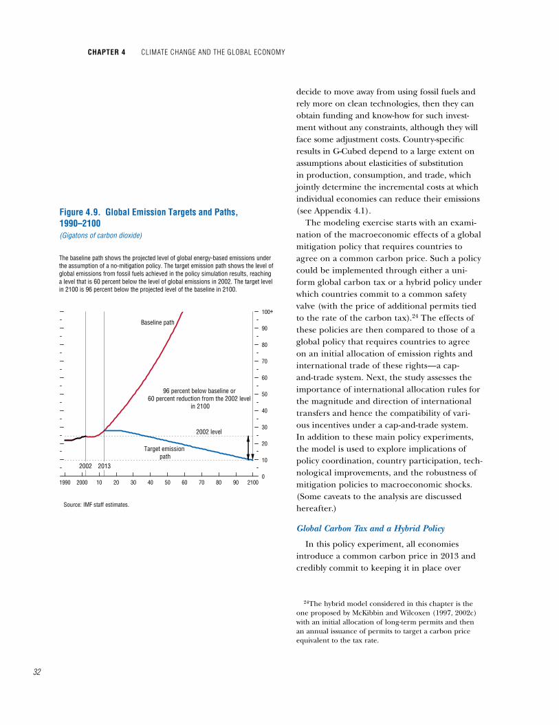
Chapter 4 Climate Change and the global eConomy
��
decide to move away from using fossil fuels and rely more on clean technologies, then they can obtain funding and know-how for such invest-ment without any constraints, although they will face some adjustment costs. Country-specific results in G-Cubed depend to a large extent on assumptions about elasticities of substitution in production, consumption, and trade, which jointly determine the incremental costs at which individual economies can reduce their emissions (see Appendix �.�).
The modeling exercise starts with an exami-nation of the macroeconomic effects of a global mitigation policy that requires countries to agree on a common carbon price. Such a policy could be implemented through either a uni-form global carbon tax or a hybrid policy under which countries commit to a common safety valve (with the price of additional permits tied to the rate of the carbon tax).�� The effects of these policies are then compared to those of a global policy that requires countries to agree on an initial allocation of emission rights and international trade of these rights—a cap-and-trade system. Next, the study assesses the importance of international allocation rules for the magnitude and direction of international transfers and hence the compatibility of vari-ous incentives under a cap-and-trade system. In addition to these main policy experiments, the model is used to explore implications of policy coordination, country participation, tech-nological improvements, and the robustness of mitigation policies to macroeconomic shocks. (Some caveats to the analysis are discussed hereafter.)
Global Carbon Tax and a Hybrid Policy
In this policy experiment, all economies introduce a common carbon price in �0�� and credibly commit to keeping it in place over
��The hybrid model considered in this chapter is the one proposed by McKibbin and Wilcoxen (�997, �00�c) with an initial allocation of long-term permits and then an annual issuance of permits to target a carbon price equivalent to the tax rate.
1990 2000 10 20 30 40 50 60 70 80 90 21000
10
20
30
40
50
60
70
80
90
100
Source: IMF staff estimates.
Figure 4.9. Global Emission Targets and Paths, 1990–2100(Gigatons of carbon dioxide)
The baseline path shows the projected level of global energy-based emissions underthe assumption of a no-mitigation policy. The target emission path shows the level ofglobal emissions from fossil fuels achieved in the policy simulation results, reachinga level that is 60 percent below the level of global emissions in 2002. The target levelin 2100 is 96 percent below the projected level of the baseline in 2100.
2013
Baseline path
Target emission path
2002 level
96 percent below baseline or 60 percent reduction from the 2002 level
in 2100
2002
+

��
the long run, adjusting the rate as necessary to achieve the profile of global emissions depicted in Figure �.9. Global emissions are assumed to follow a mildly hump-shaped path, peaking around �0�8 and then gradually declining to �0 percent of the �00� levels by ��00 (that is, a �0 percent reduction from the �00� levels or a 9� percent reduction from the business-as-usual baseline that assumes no policy change).�� The carbon price rises gradually over time, reaching $8� a ton by �0�0 (an average annual rate of about $� per ton of carbon).�� This corresponds to a $0.�� increase in the price of a gallon of gasoline by �0�0 and a $�8 increase in the price of a short ton of bituminous coal. The price is imposed upstream in the fuel production chain, with revenues from carbon pricing used to fund government consumption and investment, and with the budget deficit and debt held constant (Appendix �.�). Other energy pricing policies are assumed to remain intact.
The macroeconomic effects of the carbon tax and the hybrid system with a safety valve are equivalent in this experiment and are depicted in Figure �.�0. (Note, however, that carbon taxes and hybrid policies generally are not equiva-
��The profile broadly matches the characteristics of the profiles shown as “Category III” in the Fourth Assess-ment Report of Working Group III of the IPCC (�007): peaking during �0�0–�0, and stabilizing CO�–equivalent concentrations in the range of ���–�90 parts per million (ppm) by volume by ��00. The scenario corresponds to a temperature increase of approximately �.8°C –�.�°C by ��00.
��By ��00, carbon prices are projected to rise to $��8 a ton of carbon. These estimates are lower, for comparable experiments, than those obtained by Nordhaus (�007a) and US CCSP (�007), where carbon prices range from $�00 to $�,000 in ��00. The difference stems mainly from the assumption of free capital flows in G-Cubed and a more flexible technological structure, both of which facilitate an efficient adaptation by firms and individu-als to higher carbon prices. Further, G-Cubed models only CO� emissions from fossil fuels, which implies that smaller increases in carbon prices are needed to achieve a given reduction in emissions than in multigas models where emission reductions are specified in CO�- equivalent terms. Comparisons with US CCSP (�007) are also complicated by the fact that the studies covered by that exercise targeted radiative forcings, not concentra-tions of CO�-equivalent emissions.
Each region is assumed to introduce a carbon tax in 2013. The tax rate is common across regions and is calibrated to achieve a 60 percent reduction relative to the 2002 level in world (energy-based) carbon dioxide emissions by 2100. This corresponds to a 96 percent reduction in global emissions relative to the baseline at 2100. The emission profile is mildly hump shaped, allowing for some increases in the medium term, peaking in 2018.
Source: IMF staff estimates. Output refers to gross national product. Interest rate refers to 10-year real interest rate. For real effective exchange rate, a positive value is an appreciation relative to the baseline.
20 30 40-140-120-100-80-60-40-20
020
2013 20 30 400
20
40
60
80
100
2013 20 30 40-30
-24
-18
-12
-6
0
6
20 30 40-4
-3
-2
-1
0
1
2 Investment
20 30 40-24
-20
-16
-12
-8
-4
0
4
2013 20 30 40-1.0
-0.8
-0.6
-0.4
-0.2
0.0
0.2Interest Rate(percentage points)
2013 20 30 40-1
0
1
2
3
20 30 40-20
-15
-10
-5
0
5
10 Real Effective Exchange Rate Current Account(percent of GDP; percentage points)
Consumption
Output
Emissions Carbon Price(U.S. dollars per tonof carbon)
Other emerging and developing economiesEastern Europe and RussiaUnited States Japan ChinaW. Europe OPEC
1
Figure 4.10. Uniform Carbon Tax, 2013–40(Deviation from the baseline; percent unless otherwise stated)
1
2013
2013
2013
2013
how Can Countries effeCtively and effiCiently mitigate Climate Change?

Chapter 4 Climate Change and the global eConomy
��
lent.)�7 Firms change their technology, substitut-ing away from carbon-intensive inputs and into capital (including noncarbon alternative tech-nologies), materials, and labor. Households alter their consumption patterns, also substituting away from carbon-intensive goods. With higher carbon prices raising costs for firms, productiv-ity and output fall. Aggregate investment falls because the average marginal product of capital is lower in each region, while consumption declines, following real incomes. Policy would be more effective to the extent that firms and households are forward looking and react imme-diately to the anticipated future prices. Although the levels of real activity fall permanently relative to the baseline, the shock has only a temporary effect on GNP growth rates: over time they return to baseline levels.�8
Changes in national levels of GNP and con-sumption reflect countries’ emission-reduction commitments and the costs of an incremental reduction in emissions. Each economy’s mar-ginal abatement costs (MACs) in G-Cubed depend on how intensely it uses carbon-based energy to produce goods for domestic consump-tion and for export, which in turn are driven by such factors as energy efficiency, factor endow-ments, and the production and export structure. China, Organization of Petroleum Exporting Countries (OPEC) members, and the United States have low MACs. MACs for eastern Europe and Russia and other emerging and developing economies are in the middle range, and MACs for Japan and western Europe are high. China is
�7The hybrid policy is not equivalent to the carbon tax under conditions of uncertainty about abatement costs. In a scenario of slower-than-expected growth, the carbon price would fall under the hybrid policy and would remain constant under the tax. Hybrid policies may differ from carbon taxes in other respects as well, for example, in how emission reduction targets are achieved or how new information on damages from climate change is reflected in carbon prices. For a more detailed discussion of hybrid policies, see McKibbin and Wilcoxen (�997, �00�a) and Aldy and Stavins (�007).
�8The study uses GNP as a measure of output. It is a better comparator of each region’s fortunes under differ-ent mitigation policies, because, unlike GDP, it takes into account transfer payments.
United Japan Western Eastern China Other OPEC World, World,-15
-10
-5
0
5
United Japan Western Eastern China Other OPEC World, World,-3
-2
-1
0
1
2Consumption
Figure 4.11. Total Costs of Mitigation, 2013–40(Deviation of the net present value from the baseline, percent)
This figure shows the costs of mitigation for the three policies shown in Figures 4.10, 4.12, and 4.14. The first panel shows the net present value of the difference between the path for real consumption in the policy experiment and the path for real consumption in the baseline, divided by the net present value of the path for real consumption in the baseline. The bottom panel shows the net present value of output (real gross national product) losses, defined in the same way as for consumption. The discount rate is constant over time and across regions at 2.2 percent, which is the difference between long-term world interest rates and trend GNP growth rates.
Uniform carbon tax and hybrid policyCap-and-trade system, allocation by initial emission sharesCap-and-trade system, allocation by population shares
States Europeand Russia
emerging anddevelopingeconomies
GNP Population1
2 3Europe
States Europeand Russia
emerging anddevelopingeconomies
GNP Population
Output
12 3Europe
Source: IMF staff estimates. Organization of Petroleum Exporting Countries. Weighted by GNP shares in 2013. Weighted by population shares in 2013. Average prices of GNP and consumption can differ widely, owing to exchange rate movements. This implies that the rankings of GNP and consumption losses across countries are not necessarily the same.
1234
4
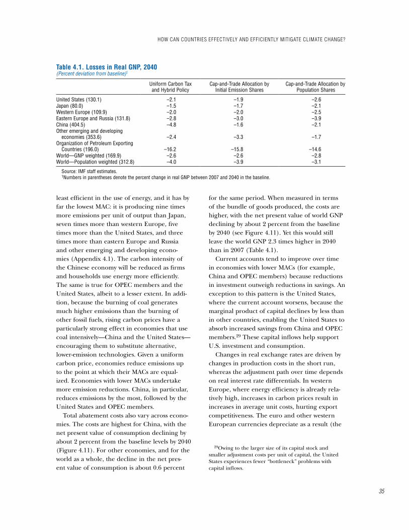
��
least efficient in the use of energy, and it has by far the lowest MAC: it is producing nine times more emissions per unit of output than Japan, seven times more than western Europe, five times more than the United States, and three times more than eastern Europe and Russia and other emerging and developing econo-mies (Appendix �.�). The carbon intensity of the Chinese economy will be reduced as firms and households use energy more efficiently. The same is true for OPEC members and the United States, albeit to a lesser extent. In addi-tion, because the burning of coal generates much higher emissions than the burning of other fossil fuels, rising carbon prices have a particularly strong effect in economies that use coal intensively—China and the United States—encouraging them to substitute alternative, lower-emission technologies. Given a uniform carbon price, economies reduce emissions up to the point at which their MACs are equal-ized. Economies with lower MACs undertake more emission reductions. China, in particular, reduces emissions by the most, followed by the United States and OPEC members.
Total abatement costs also vary across econo-mies. The costs are highest for China, with the net present value of consumption declining by about � percent from the baseline levels by �0�0 (Figure �.��). For other economies, and for the world as a whole, the decline in the net pres-ent value of consumption is about 0.� percent
for the same period. When measured in terms of the bundle of goods produced, the costs are higher, with the net present value of world GNP declining by about � percent from the baseline by �0�0 (see Figure �.��). Yet this would still leave the world GNP �.� times higher in �0�0 than in �007 (Table �.�).
Current accounts tend to improve over time in economies with lower MACs (for example, China and OPEC members) because reductions in investment outweigh reductions in savings. An exception to this pattern is the United States, where the current account worsens, because the marginal product of capital declines by less than in other countries, enabling the United States to absorb increased savings from China and OPEC members.�9 These capital inflows help support U.S. investment and consumption.
Changes in real exchange rates are driven by changes in production costs in the short run, whereas the adjustment path over time depends on real interest rate differentials. In western Europe, where energy efficiency is already rela-tively high, increases in carbon prices result in increases in average unit costs, hurting export competitiveness. The euro and other western European currencies depreciate as a result (the
�9Owing to the larger size of its capital stock and smaller adjustment costs per unit of capital, the United States experiences fewer “bottleneck” problems with capital inflows.
table 4.1. losses in real gnp, 2040(Percent deviation from baseline)1
Uniform Carbon Tax and Hybrid Policy
Cap-and-Trade Allocation byInitial Emission Shares
Cap-and-Trade Allocation byPopulation Shares
United States (130.1) –2.1 –1.9 –2.6Japan (80.0) –1.5 –1.7 –2.1Western Europe (109.9) –2.0 –2.0 –2.5Eastern Europe and Russia (131.8) –2.8 –3.0 –3.9China (404.5) –4.8 –1.6 –2.1Other emerging and developing
economies (353.6) –2.4 –3.3 –1.7Organization of Petroleum Exporting
Countries (196.0) –16.2 –15.8 –14.6World—GNP weighted (169.9) –2.6 –2.6 –2.8World—Population weighted (312.8) –4.0 –3.9 –3.1
Source: IMF staff estimates. 1Numbers in parentheses denote the percent change in real GNP between 2007 and 2040 in the baseline.
how Can Countries effeCtively and effiCiently mitigate Climate Change?
Chapter 4 Climate Change and the global eConomy
��
euro by about �� percent during �0��–�0). By contrast, in China, the marginal costs of reduc-ing emissions are low, and increases in carbon prices can be largely offset by improvements in energy efficiency. The resulting terms-of-trade improvement is reflected in an exchange rate appreciation.
MACs and emission reductions per dollar increase in carbon prices are similar to those obtained by Nordhaus (�007a) but lower than those in many other models (for example, US CCSP, �007). This is true for three reasons. First, in contrast to models that assume tech-nologies in which energy can be used only in fixed proportions with other inputs of produc-tion, G-Cubed allows for substitution between factors of production. Second, forward-looking expectations in G-Cubed make carbon price increases more effective in lowering emissions. The third factor driving down cost estimates is that G-Cubed explicitly models international capital flows, in contrast to most other models in the literature (Appendix �.�). Free flow of capital implies that capital moves to economies with higher MACs, facilitating both the replace-ment of old capital stock and the transition to low-emission technology, and allowing the sav-ings of economies with lower MACs to go where expected returns are higher.
The total costs of mitigation in G-Cubed are higher than in many other studies, but they are within the range of estimates reported in IPCC (�007).�0 The main reasons this analysis yields higher estimates is that it assumes relatively strong emission growth in the baseline (bench-marked in IEA, �007a), and that G-Cubed uses conservative assumptions about the availability of so-called backstop technologies with zero emissions. In many other studies, GDP losses are substantially reduced or even eliminated by �0�0 because innovation and the diffusion of backstop technologies and other low-emission
�0In this study, mitigation policies reduce world GDP by �.8 percent by �0�0 compared with the business-as-usual baseline. The range of estimates reported in IPCC (�007) is 0 to � percent.
technologies are assumed to proceed rapidly, at a faster pace than in G-Cubed (for example, US CCSP, �007; Criqui and others, �00�; den Elzen and others, �00�; and Nakicenovic and Riahi, �00�).��
A Global Cap-and-Trade System
This experiment assumes that a permanent cap-and-trade policy is put in place in �0��. Emission rights for the world as a whole are assumed to follow the emission profile shown in Figure �.9—by �0�0 the world is allowed to emit only �0 percent of the �00� emission levels. Individual economies receive emission rights for each year from �0�� onward. These rights are proportional to the economy’s share of global emissions in �0��, following the profile depicted in Figure �.9. Emission permits can be traded internationally, which establishes a common price.�� Economies with higher MACs buy permits from economies with lower MACs, compensating them for undertaking more abate-ment than implied by their share of emissions. Hence, the actual emission paths of individual economies differ from their initial allocations of permits, whereas the world emission path is consistent with the targeted profile.
The macroeconomic effects of the global cap-and-trade system are similar to those of the global carbon tax and the hybrid policy with a safety valve, with differences reflecting the various mechanisms through which a common carbon price is established (Figure �.��). Under the global tax, countries are assumed to agree on a common carbon price, whereas under the
��The carbon tax system considered in this study does not require international transfers: governments are assumed to agree on a common tax rate. In practice, however, the establishment of such a system may require side payments, which would alter macroeconomic out-comes. Border tax adjustments also may be used as a way to induce other countries to participate, albeit at the risk of a protectionist response.
��Emission permits are allocated to governments, which then sell them to the private sector. Firms are free to trade permits internationally. Governments spend revenues from permit auctioning on consumption and investment, keeping deficits unchanged.

��
global cap-and-trade system, a common carbon price is established through international trade in emission permits. For most economies, trans-fers are small and hence the macroeconomic effects are similar; for China (a recipient), other emerging and developing economies (payers), and OPEC members (recipients), transfers reach about �0 percent, –� percent, and � percent of GDP, respectively, by �0�0 (Figure �.��). China receives the largest transfers because it is com-paratively inefficient in the use of energy and can reduce emissions at much lower costs than other economies. Advanced economies, as well as other emerging and developing economies, buy emission rights from China because emis-sion reductions are very costly for them. The above findings concerning the direction and magnitude of transfers are highly sensitive to marginal abatement costs assumed in G-Cubed for individual economies (see Appendix �.�) as well as to the rule used for allocating permits across countries (see below).
Differences in the macroeconomic effects of a global cap-and-trade system, a global carbon tax, and the hybrid with a safety valve are thus most vivid for China. China’s consumption rises under a cap-and-trade system, but declines under a carbon tax and under the hybrid (see Figure �.��). Under cap and trade, the current account remains broadly stable for the first �0 years (and gradually improves after that); there would be an immediate improvement under both a carbon tax and the hybrid (see Fig-ure �.�0). International transfers also result in a larger real appreciation of the renminbi under cap and trade (�0 percent by �0�0 compared with � percent under a carbon tax and the hybrid).
Total (GNP-weighted) world abatement costs are similar under a cap-and-trade system, a car-bon tax, and the hybrid policy, but the popula-tion-weighted costs are higher under cap and trade, because the increase in costs for other emerging and developing economies outweighs the decrease in costs for China. The costs for economies paying transfers (Europe, Japan, Russia, and other emerging and developing
Each region is assumed to introduce a cap-and-trade system in 2013. Each region has to achieve a 60 percent reduction relative to the 2002 level in world (energy-based) carbon dioxide emissions by 2100, but is able to buy and sell emission permits to do so. This corresponds to a 96 percent reduction in global emissions relative to the baseline at 2100. Each region’s emission target is mildly hump shaped, allowing for some increases in the medium term, peaking in 2018.
2013 20 30 40-1
0
1
2
3
4
2013 20 30 40-2.0
-1.5
-1.0
-0.5
0.0
0.5
2013 20 30 40-30
-25
-20
-15
-10
-5
0
5
2013 20 30 400
20
40
60
80
100
Source: IMF staff estimates. Output refers to gross national product. Interest rate refers to 10-year real interest rate. For real effective exchange rate, a positive value is an appreciation relative to the baseline.
Carbon Price(U.S. dollars per tonof carbon)
Investment
20 30 40-20
-15
-10
-5
0
5
20 30 40-3
-2
-1
0
1
2
3
20 30 40-140-120-100-80-60-40-20
020
Consumption
Output Interest Rate(percentage points)
20 30 40-25-20
-15-10
-505
1015 Real Effective Exchange Rate Current Account
(percent of GDP; percentage points)
Emissions
Figure 4.12. Cap-and-Trade System, 2013–40(Deviation from the baseline; percent unless otherwise stated)
1
1
2013
2013
2013
2013
Other emerging and developing economiesEastern Europe and RussiaUnited States Japan ChinaW. Europe OPEC
how Can Countries effeCtively and effiCiently mitigate Climate Change?
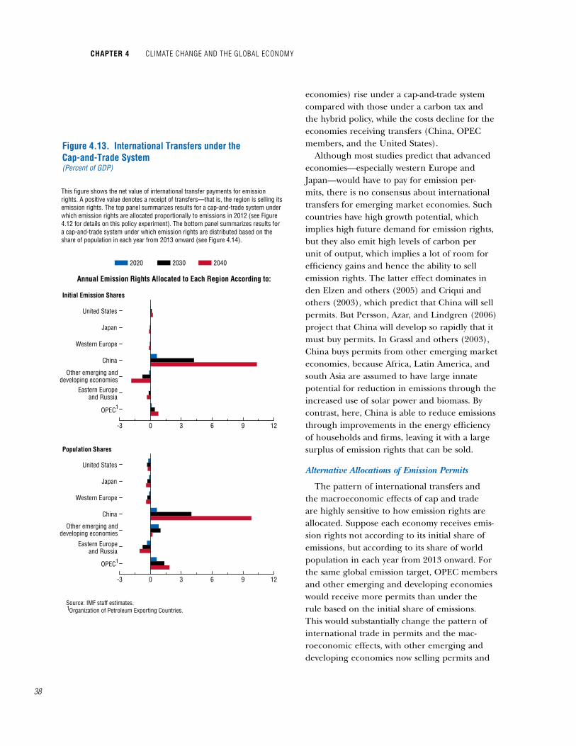
Chapter 4 Climate Change and the global eConomy
��
economies) rise under a cap-and-trade system compared with those under a carbon tax and the hybrid policy, while the costs decline for the economies receiving transfers (China, OPEC members, and the United States).
Although most studies predict that advanced economies—especially western Europe and Japan—would have to pay for emission per-mits, there is no consensus about international transfers for emerging market economies. Such countries have high growth potential, which implies high future demand for emission rights, but they also emit high levels of carbon per unit of output, which implies a lot of room for efficiency gains and hence the ability to sell emission rights. The latter effect dominates in den Elzen and others (�00�) and Criqui and others (�00�), which predict that China will sell permits. But Persson, Azar, and Lindgren (�00�) project that China will develop so rapidly that it must buy permits. In Grassl and others (�00�), China buys permits from other emerging market economies, because Africa, Latin America, and south Asia are assumed to have large innate potential for reduction in emissions through the increased use of solar power and biomass. By contrast, here, China is able to reduce emissions through improvements in the energy efficiency of households and firms, leaving it with a large surplus of emission rights that can be sold.
Alternative Allocations of Emission Permits
The pattern of international transfers and the macroeconomic effects of cap and trade are highly sensitive to how emission rights are allocated. Suppose each economy receives emis-sion rights not according to its initial share of emissions, but according to its share of world population in each year from �0�� onward. For the same global emission target, OPEC members and other emerging and developing economies would receive more permits than under the rule based on the initial share of emissions. This would substantially change the pattern of international trade in permits and the mac-roeconomic effects, with other emerging and developing economies now selling permits and
United States
Japan
Western Europe
China
Less developed count
Eastern Europe
OPEC
-3 0 3 6 9 12
United States
Japan
Western Europe
China
Less developed count
Eastern Europe
OPEC
-3 0 3 6 9 12
Initial Emission Shares
Source: IMF staff estimates. Organization of Petroleum Exporting Countries.
Other emerging anddeveloping economies
Annual Emission Rights Allocated to Each Region According to:
Population Shares
This figure shows the net value of international transfer payments for emission rights. A positive value denotes a receipt of transfers—that is, the region is selling its emission rights. The top panel summarizes results for a cap-and-trade system under which emission rights are allocated proportionally to emissions in 2012 (see Figure 4.12 for details on this policy experiment). The bottom panel summarizes results for a cap-and-trade system under which emission rights are distributed based on the share of population in each year from 2013 onward (see Figure 4.14).
Figure 4.13. International Transfers under the Cap-and-Trade System(Percent of GDP)
2020 2030 2040
Eastern Europeand Russia
Eastern Europeand Russia
Other emerging anddeveloping economies
OPEC1
OPEC1
1

��
receiving transfers in the amount of about � per-cent of GDP during �0�0–�0 (see Figure �.��). Transfers to OPEC members would also rise to about � percent of GDP in �0�0, whereas those to China would remain broadly unchanged.
Transfers to other emerging and developing economies would improve their consumption outcomes, but would lead to real exchange rate appreciation and a phenomenon akin to Dutch disease (Figure �.��). Agriculture and services sectors in other emerging and developing economies would experience a larger contrac-tion than under the emission-based cap-and-trade system. Appreciation would persist during several decades following the introduction of the population-based cap and trade.
Nonetheless, when measured in GNP-weighted terms, world abatement costs would be similar under a population-based cap and trade, under an emission-based cap-and-trade system, and under a uniform global carbon tax, reflect-ing similar outcomes in terms of increased energy efficiency. In population-weighted terms, world costs decline owing to consumption benefits now accruing to other emerging and developing economies and OPEC members (see Figure �.��).
Other Findings
Nonharmonized mitigation policies—for example, under which each economy indepen-dently chooses its own path for carbon prices in order to achieve a �0 percent reduction from �00� emission levels by ��00—would be more costly than harmonized policies because they do not provide for an efficient allocation of abatement across the world (Nordhaus, �007a). Under G-Cubed simulations, total costs at least double for other emerging and developing economies, eastern and western Europe, Rus-sia, and Japan, compared with the costs of the uniform global carbon tax. Although China, OPEC, and the United States would have lower costs than under a uniform carbon tax, the total global costs of uncoordinated policies are still �0 percent higher than those of harmonized policies. Countries with higher MACs would
Beginning in 2013, there is a cap-and-trade system for all regions to gradually achieve 60 percent reductions in total world (energy-based) carbon dioxide emissions relative to the 2002 level by 2100, allowing for some increases in the medium term, peaking in 2018. This corresponds to a 96 percent reduction in global emissions relative to the baseline at 2100. Emission rights are allocated by share of global population in each year from 2013 onward.
Source: IMF staff estimates. Output refers to gross national product. Interest rate refers to 10-year real interest rate. For real effective exchange rate, a positive value is an appreciation relative to the baseline.
2013 20 30 40-30
-25
-20
-15
-10
-5
0
5
2013 20 30 40-2.0
-1.5
-1.0
-0.5
0.0
0.5
20 30 40-20
-15
-10
-5
0
5
2013 20 30 400
20
40
60
80
100
20 30 40-3
-2
-1
0
1
2
3 Investment
Carbon Price(U.S. dollars per tonof carbon)
20 30 40-140-120-100-80-60-40-20
020
Consumption
Output Interest Rate(percentage points)
2013 20 30 40-1
0
1
2
3
4
20 30 40-20
-15
-10
-5
0
5
10 Real Effective Exchange Rate Current Account(percent of GDP; percentage points)
Emissions
Figure 4.14. Cap-and-Trade System for All Regions Based on Share of World Population, 2013–40(Deviation from the baseline; percent unless otherwise stated)
1
1
2013
2013
2013
2013
Other emerging and developing economiesEastern Europe and RussiaUnited States Japan ChinaW. Europe OPEC
how Can Countries effeCtively and effiCiently mitigate Climate Change?

Chapter 4 Climate Change and the global eConomy
�0
be particularly adversely affected by the lack of policy coordination, because these countries would no longer be able to relocate abatement to other destinations. This policy experiment suggests that an international policy architecture based on country-specific carbon prices would be less efficient than an architecture establishing a common world carbon price.
An international agreement that does not include emerging and developing economies will be ineffective in stemming climate change. If only Annex I economies�� (Australia, Canada, eastern and western Europe, Japan, New Zea-land, Russia, and the United States) were to assume the full burden of reducing world emis-sions by �0 percent from �00� levels by ��00, their emissions would need to be ��!/2 times lower than in the baseline. This is because they would need to offset the large contribution of non-Annex I countries (China and other emerg-ing and developing economies) to the growth of world emissions. This would represent an unrealistically high cost to Annex I economies. Alternatively, if only Annex I economies decided to reduce their total emissions by �0 percent by ��00, global emissions would be 7!/2 times higher than in �00�, resulting in greater warming.
The carbon tax and the hybrid policy with a safety valve provide more flexibility for firms and households to respond to fluctuations in abatement costs stemming, for example, from changes in the rate of economic growth. During periods of cyclically high demand and expand-ing production, cap and trade may become too restrictive, requiring firms to abate to the same extent despite higher abatement costs. When one region experiences unexpectedly higher growth, this would drive up the price of carbon permits for all countries, with the result that those countries that were previously net beneficiaries of transfer payments might find themselves having to pay (McKibbin and
��Annex I of the Kyoto Protocol lists the assigned emis-sion targets over the commitment period �008–��. This does not necessarily mean that the emission targets have been agreed to or met.
Wilcoxen, �00�). If carbon prices are volatile, variations in growth may put a stress on a global cap-and-trade agreement. This is not the case under the carbon tax or the hybrid policy.��
This policy experiment also illustrates that mitigation policies may have important implica-tions for the way macroeconomic shocks are transmitted across countries. For example, under a price-setting policy, unanticipated growth spills over positively to other countries, although this implies that the world misses its emission targets. By contrast, under the global cap-and-trade system, the world global emission target can be achieved, but higher economic growth in one large economy may have negative repercussions across other countries by driving up permit prices.
Energy-efficiency improvements are unlikely to eliminate the need for carbon prices, but they would reduce their level (Nordhaus, �007a). Even assuming that energy efficiency exog-enously improves at a pace that is twice as high as in the baseline, carbon prices would still need to rise to achieve the same reduction in emis-sions (the carbon price would need to reach $7� by �0�0, instead of $8�, as in the original policy experiments with the global price-based policies). This points to the potential benefits of complementing carbon pricing with well-designed incentives for innovation and the broad diffusion of clean technologies (see Box �.�).
Less-stringent emission targets—aiming to stabilize GHG concentrations at about ��0 ppm in CO�e terms, rather than ��0 ppm, by ��00—would be less costly to achieve, but the differ-ence in costs would not be dramatic. Analysis of an alternative mitigation scenario, under which emissions were only �0 percent below �00� levels by ��00 and were allowed to continue to grow for longer before declining,�� shows that
��The hybrid has a number of advantages under uncer-tainty, such as directly addressing the problem of time consistency that arises under the cap-and-trade system and carbon-tax approaches.
��Matching the “Category IV” scenarios in IPCC (�007) and corresponding to �90–7�0 ppm in CO�e terms.
��
the patterns of macroeconomic responses under carbon taxes, hybrid policies, and cap-and-trade systems remain largely unchanged. However, under the less-stringent scenario, carbon prices would rise more slowly, to $��� by ��00, imply-ing slightly lower consumption and GNP losses (of about 0.� percent and �.7 percent in net present value, respectively).
Caveats
Several caveats need to be underlined. The most important is that it is difficult to say anything precise about the state of the world economy and individual country economies in �0�0, let alone ��00, especially if there are large and fundamental changes in the price of energy. Many innovations in technology could occur that would change the outlook dramati-cally over several decades, and these innovations could diffuse at different rates across countries. Results are most sensitive to assumptions about economic growth, autonomous energy-efficiency improvements, and marginal abatement costs—small changes in these assumptions can have a big impact on results in G-Cubed. The direction and magnitude of macroeconomic effects for individual countries, including financial trans-fers, are particularly sensitive to assumptions about elasticities of substitution in production, consumption, and trade. Using only current technologies, many firms may be unable to react to market demand to the extent estimated in this analysis; yet by basing many of the estimates of the price responsiveness of households and firms on historical experience through econo-metric estimation, the model attempts to reflect plausible outcomes in technological change. Although G-Cubed does not model when backstop technologies would emerge, it assumes that changes in carbon prices can induce large substitutions away from fossil fuels. Many other models have more rigid technological struc-tures or assume that capital and technology do not flow freely across countries, even over the long run. At the same time, by focusing only on energy-related CO� emissions, G-Cubed does not take into account cheap abatement opportuni-
ties that may exist in other areas, for example, by reducing deforestation.
ConclusionsClimate change is a powerful global trend
that, along with trade and financial integration, is likely to have profound effects on economies and markets in coming decades. As tempera-tures and sea levels rise and precipitation pat-terns change, the global pattern of comparative advantage will shift in tandem. This will prompt structural changes within economies, at the domestic as well as at the global level. There will be shifts in international trade, in capital and migration flows, and in the prices of commodi-ties, other goods and services, and assets.
The macroeconomic effects of climate change will unfold unevenly across time and space. Poor countries will be hit earlier and harder, owing to their geography, heavier reliance on agricul-ture, and more limited capacity to adapt. Their health and water systems may come under stress from more frequent natural disasters, coasts may be flooded, and populations may migrate. Rich countries may be affected by spillovers from cli-mate change in poor countries, and they would also face severe direct damage if the tail risks of climate catastrophes were to materialize.
The ability of domestic macroeconomic poli-cies to help public and private sectors cope with climate-related risks will be increasingly tested over time. Sound macroeconomic policies and innovative financial and development strategies will be needed to help countries successfully adapt to climate change. Countries with higher incomes, stronger fiscal positions, more devel-oped financial markets, and greater structural policy flexibility will be better positioned to adapt to the adverse consequences of climate change. Countries that are increasingly subject to risks from weather volatility and extreme weather events will need to devise strategies for managing such risks, including the appropri-ate use of self-insurance through budgetary management, the building of reserves, and the use of weather derivatives, catastrophe bonds,
ConClusions
Chapter 4 Climate Change and the global eConomy
��
and other forms of disaster insurance. Global cooperation in transferring knowledge about the financial management of weather-related risks would help poor countries better adapt to climate change.
Dealing with climate change also poses enormous multilateral policy challenges. These range from fostering synergies in adaptation and protecting the natural environment to preserv-ing energy security and managing the risks of protectionism. Yet the main task is to address the causes and impacts of climate change by signifi-cantly reducing emissions of GHGs over the next several decades, and to do this at the lowest pos-sible cost. This requires joint action by advanced, emerging market, and developing economies.
This chapter concludes that climate change can be addressed without imposing heavy damages either on the global economy or on individual countries. For climate policies to be successful, their potentially adverse economic consequences—slower growth, higher inflation, loss of competitiveness—must be addressed, either through carefully designed climate poli-cies or through supportive macroeconomic and financial policies. Measures to limit the adverse economic effects would strengthen the incen-tives for a broad range of countries to fully participate in mitigation efforts and would help unleash the potential economic and financial benefits of the transition to a more climate-friendly global economy.• Carbon-pricing policies need to be long term
and credible. They must establish a time horizon for steadily rising carbon prices that people and businesses consider believable. Increases in world carbon prices need not be large—say a $0.0� initial increase in the price of a gallon of gasoline that rises by $0.0� every three years. Such gradual increases, if started early, would allow the cost of adjust-ment to be spread over a longer period of time. The total cost to the global economy of such policies could be moderate for policies introduced in �0�� that aim to stabilize CO�e concentrations at ��0 ppm by ��00—entailing only a 0.� percent reduction in the net pres-
ent value of world consumption by �0�0. Even with this loss, world GNP would still be �.� times higher in �0�0 than in �007.
• Carbon-pricing policies should induce all groups of economies—advanced, emerg-ing, and developing—to start pricing their emissions. Any policy framework that does not include emerging and developing econo-mies (particularly, large and fast-growing economies such as Brazil, China, India, and Russia) in some way (for example, with a lag or with initially less-stringent targets) would be extremely costly and would be politically untenable. That is because during the next �0 years, 70 percent of emissions are projected to come from these and other emerging and developing economies. Some countries may need to strengthen their institutional capacity, however, to implement carbon pricing.
• Carbon-pricing policies should strive to estab-lish a common world price for emissions. This would ensure that emission reduction occurs where it is least costly to do so. Emerging and developing economies, in particular, will likely be able to reduce emissions much more cheaply than advanced economies. For exam-ple, if China and India have access to technol-ogies similar to those available in Europe and Japan, they could cut emissions dramatically by improving their intensity of energy use and by reducing their reliance on coal. The difference in costs can be significant—for the world as a whole, costs would be �0 percent lower if carbon prices were the same across countries. Countries would either need to agree to harmonize the rate of a carbon tax, coordinate trigger prices for the safety valve under a hybrid policy, or allow international trading of emission permits under a cap-and-trade system.
• Carbon-pricing policies should be sufficiently flexible to accommodate cyclical economic fluctuations. During periods of high demand, for example, it would be more costly for firms to reduce their emissions, and the opposite would be true when demand is low. Abate-ment costs would be lower if firms could vary
��
their emissions over the business cycle. That would allow a given average level of emission reductions to be achieved over the medium term. In contrast to carbon taxes and hybrid policies, a cap-and-trade system could prove restrictive in periods of higher growth owing to increased demand and prices for emission permits, unless it incorporates elements that help control price volatility.
• The costs of mitigation should be distributed equitably across countries. Some mitigation policies—for example, a uniform tax, a cap-and-trade system under which permits are allocated based on countries’ current shares of emissions, or a hybrid policy combining elements of the two—would impose high costs on some emerging and developing econo-mies. Substantial cross-border transfers may be needed to encourage them to participate and to help them deal with the negative impact. The direction and magnitude of trans-fers under cap and trade generally depend on the incremental costs of reducing emissions in individual countries (which in turn are a function of countries’ domestic technological capabilities and access to foreign technology) as well as on the specific design features of mitigation policies (for example, rules for allocating emission permits, the timing of countries’ entry into the climate agreement, supplementary conditions, and the like). If policies were designed so that transfers flow from advanced economies to emerging and developing economies, this would reduce the costs of carbon-pricing policies for the latter two groups, encouraging them to participate. Using border tax adjustments as a way to induce countries to join could elicit a pro-tectionist response that would detract from mitigation efforts. In addition, countries may need to comple-
ment carbon pricing with appropriate macro-economic and financial policies. For example, under a global cap-and-trade system, transfers from economies that buy permits to economies that sell them could be potentially large—for example, several percentage points of GDP.
Such transfers may cause real exchange rates in the recipient countries to appreciate consider-ably, making some sectors of their economies less competitive—Dutch disease. Such macroeco-nomic effects can be reduced if countries save a portion of these inflows, continue to improve their business environments, and, depending on their exchange rate regimes, allow appreciation to take place at least partly through the nominal exchange rate rather than through inflation.
This chapter also points to the supporting role of international capital movements and technology transfer in dealing with climate change. Capital and technology flows can reduce the costs of mitigation by helping allo-cate abatement to the least costly destinations, while making abatement easier through the use of modern technology. Initiatives by major advanced economies to subsidize the transfer of clean technologies to emerging and developing economies can complement a global commit-ment to contain carbon emissions through a broadly accepted global carbon-pricing frame-work. While unlikely to eliminate the need for carbon pricing, well-designed incentives for innovation and the diffusion of clean technolo-gies can help reduce the costs of addressing climate change.
Climate change is a complex global problem that does not lend itself to easy policy solutions. This chapter does not pretend to provide a solu-tion. Its focus has been narrow—on the cross-country macroeconomic dimensions of climate change. Yet its conclusion has broad relevance for ongoing policy debates: climate change can be addressed with minimum damage to the economy, if policy solutions follow some basic principles.
appendix 4.1. the g-Cubed model, baseline assumptions, and other models in the Climate Change literatureThe main author of this appendix is Alasdair Scott.
This appendix outlines the key features of the model used to produce the analysis in Chap-
appendix 4.1. the g-Cubed model, baseline assumptions, and other models in the Climate Change literature
Chapter 4 Climate Change and the global eConomy
��
ter �, the baseline scenario and its underlying assumptions, the factors affecting the differences in marginal abatement costs (MACs) across countries, and comparisons with some other models that have been prominently used in the literature on climate change mitigation.
the g-Cubed model
G-Cubed (see McKibbin and Wilcoxen, �998) is a dynamic general equilibrium model of the global economy. The world is divided into multiple regions linked by international trade and capital flows, with each region divided into multiple production sectors. Decisions about saving, investment, and asset pricing are mod-eled by assuming that forward-looking house-holds and firms aim to maximize, respectively, consumption utility and profits, but are subject to cash flow constraints, while backward-look-ing households and firms follow simple rules of thumb.�� Outputs of different sectors are linked to emissions of carbon dioxide using data for the emission intensity and the energy efficiency of each sector.
Some of the key features of G-Cubed relevant for this study include the following:• disaggregation of the real sector into an
input-output structure to allow for produc-tion and trade of multiple goods and services within and across economies, facilitating the examination of how changes in energy prices are transmitted within and across economies;
• “stock-flow” accounting for capital stock and financial assets and enforcement of cash flow and budget constraints;
• integration of real and financial markets, including the modeling of international capi-tal flows along with trade balances; and
��Thirty percent of households are forward looking and 70 percent follow rules of thumb. Expectations play a key role in the effectiveness of carbon prices at reducing emissions, because forward-looking households will factor all future carbon price increases into their current deci-sions. Hence, for the same carbon price profile, a larger share of forward-looking households would imply earlier reductions in emissions.
• modeling of fiscal and monetary policies.The �007 version of G-Cubed used in this
study splits the world into the following nine economies:�7
• United States;• Japan;• Western Europe (Austria, Belgium, Denmark,
Finland, France, Germany, Greece, Iceland, Ireland, Italy, Luxembourg, Netherlands, Norway, Portugal, Spain, Sweden, Switzerland, and United Kingdom);
• Australia;• Canada and New Zealand;• Eastern Europe and Russia (Albania, Bulgaria,
Czech Republic, Hungary, Poland, Romania, and Russia);
• China;• other emerging and developing economies
(Argentina, Brazil, Cambodia, Chile, Egypt, Hong Kong SAR, India, People’s Democratic Republic of Korea, Republic of Korea, Lao PDR, Malaysia, Mexico, Morocco, Myanmar, Nepal, Pakistan, Philippines, Singapore, South Africa, Sri Lanka, Thailand, Turkey, and Vietnam);
• OPEC economies (Algeria, Indonesia, Islamic Republic of Iran, Iraq, Kuwait, Libya, Niger, Oman, Qatar, Saudi Arabia, and United Arab Emirates).The six economies covering Australia, Canada
and New Zealand, western Europe, eastern Europe and Russia, Japan, and the United States are broadly equivalent to the definition of Annex I under the Kyoto Protocol (United Nations, �998).
The production structure of each region is the same, with the following �� production sectors:• energy sectors: electric utilities, gas utilities,
petroleum refining, coal mining, crude oil and gas extraction; and
�7Country coverage is constrained by data limitations. Hence, the definition of the “world” may differ from that in other studies, and this may need to be taken into consideration when comparing policy scenarios.

��
• nonenergy sectors: mining; agriculture, fish-ing, and hunting; forestry and wood products; durable goods manufacturing; nondurable goods manufacturing; transportation; and services.The structure of each region is identical but
varies in the values of parameters describing shares, weights, and elasticities. Each region consists of several economic agents: households, a consolidated government, the financial sector, and the production sectors listed above. Each firm makes decisions about capital investment and the use of labor, intermediate materials, and energy so as to maximize the value of the firm, given available technology and the prices the firm faces for inputs and outputs. Labor supply is assumed to meet labor demand from firms in the short run—in the long run, it is constrained by population levels—and workers are fully mobile across sectors (they receive the same real wage). By contrast, it takes time to shift and install capital. Each household receives labor and dividend income from firms and (net) transfer income from the government. Given its period-by-period budget constraints and the prices of goods relative to income and other goods, each household makes decisions about total consumption expenditure and the way that expenditure is allocated across a basket of energy and nonenergy goods.
The government administers monetary and fiscal policy. It faces a binding period-by-period fiscal constraint, balancing revenues with expen-ditures. Each region has the same fiscal rule: given targets for tax rates, transfers, deficits, and expenditures on wages, extra revenues—such as from carbon taxes or sales of emission permits—are used to fund government con-sumption and investment. To the extent that a rise in carbon prices reduces private demand, this rule will have a small offsetting effect on aggregate demand. The main conclusions in this study are broadly robust to using alterna-tive fiscal rules.�8 There are nominal rigidi-
�8For example, the most efficient use of carbon rev-enues would be to reduce distortionary taxes on capital.
ties for prices and wages. Governments in the model can use nominal interest rates to achieve targets for inflation, money growth, nominal GDP growth, or exchange rates, or for a mix-ture of these.
An important aspect of the model is the way in which sectors and economies are linked by trade in goods and services, current transfers, and capital flows. All goods are potentially tradable, but the degree to which they are traded depends on how much they are used as inputs of production in other countries and on their relative prices, which depend in turn on their elasticities of substitution in produc-tion and consumption. Relative prices, such as terms of trade and real exchange rates, adjust to clear the worldwide market for goods and services. In addition, capital is assumed to flow freely across borders in search of the highest rate of return. Current flows include transfers from permit trades under a cap-and-trade system, in addition to investment returns on foreign assets.
Baseline Assumptions
The baseline—which is sometimes referred to in other studies as the reference path or busi-ness-as-usual (BAU) scenario—is a set of paths, for variables such as GDP and emissions, that is generated by the model and does not include any shocks other than those implicit in assump-tions about population and productivity growth and does not include any policy interventions other than those implicit in fiscal and mon-etary rules. The main assumptions that drive the baseline are those that affect underlying trend growth (here, population and productivity growth), policy assumptions (such as tax rates and spending levels), emission-related assump-tions (such as any improvements in energy efficiency), and the structure of the economies
Equity considerations might argue for a reduction in income tax rates for those with lower incomes, as carbon taxes are regressive. Alternatively, carbon revenues could be used to fund research in clean technologies or to pay down debt.
appendix 4.1. the g-Cubed model, baseline assumptions, and other models in the Climate Change literature
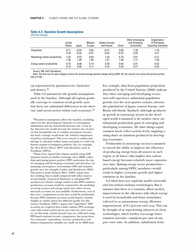
Chapter 4 Climate Change and the global eConomy
��
(as represented by parameters for elasticities and shares).�9
Table �.� summarizes the growth assumptions used in the baseline. Although all regions gradu-ally converge to common trend growth, note that there are substantial differences in the short run (and across sectors within each economy).�0
�9Parameter assumptions affect the baseline, including values for the intertemporal elasticity of consumption substitution and the household discount rate. A rise in the discount rate would increase the market rate of inter-est that households use to evaluate permanent income, but such a change would leave the ordinal comparisons of policies unchanged. This is in contrast to studies that attempt to calculate welfare losses and gains in a full cost-benefit analysis of mitigation policies. See, for example, the Stern Review (Stern, �007) and discussion, such as Nordhaus (�007a).
�0Some have argued that climate models using GDP measures based on market exchange rates (MER) rather than purchasing power parities (PPP) understate the size of emerging and developing economies and therefore, by assuming convergence, overestimate GDP and emission growth (see, for example, Castles and Henderson, �00�). This point is hotly debated. IPCC (�007) argues that the resulting bias is small compared with other sources of uncertainty. A practical limitation to adopting PPP measures for climate change studies is that PPP-consistent production accounts would be required for the modeling of energy sectors and energy inputs into other sectors, and such accounts are not available. Furthermore, even if they were, comparisons across time would be problematic because PPP-consistent accounts would impose constant weights or relative prices for different goods. For this reason, Nordhaus (�007c) argues that “superlative” PPP accounts are required that would combine PPP exchange rates with actual market prices over time for each coun-try. In this study, relative growth rates are calibrated using PPP-based national income comparisons, but projections for economies’ expenditure, income, production, and balance-of-payments variables are made on an MER basis.
For example, data from population projections produced by the United Nations (�00�) indicate that other emerging and developing econo-mies will experience substantial population growth over the next quarter century, whereas the populations of Japan, eastern Europe, and Russia will shrink. Similarly, although productiv-ity growth in nonenergy sectors in the devel-oped world is assumed to be modest, there are substantial productivity gains in emerging and developing economies. All other things equal, emission levels reflect activity levels, implying a rising share of emissions produced by develop-ing economies.
Productivity in nonenergy sectors is assumed to exceed the ability to improve the efficiency of producing energy from all sources in each region at all times—this implies that carbon-based energy becomes relatively more expensive over time. Raising energy sector productivity—particularly among OPEC members—would result in higher economic growth and higher emissions in the baseline.
G-Cubed does not explicitly model renewable and low-carbon-emission technologies. But it assumes that there is a constant, albeit modest, improvement in the efficiency with which energy is used by households and firms (sometimes referred to as autonomous energy efficiency improvement) of 0.� percent each year. This can be thought of as representing advances in clean technologies, which further encourage lower emission intensity—emissions per unit of out-put—over time. In addition, substitution from
table 4.2. baseline growth assumptions(Percent change)
United States Japan
Western Europe
Eastern Europe and Russia China
Other Developingand Emerging Economies
Organizationof Petroleum
Exporting Countries
Population 0.710.18
–0.54–0.56
0.03–0.07
–0.57–0.53
0.08–0.23
1.290.20
1.180.27
Nonenergy sector productivity 1.551.56
0.521.49
0.621.50
1.551.57
6.781.58
2.611.71
0.721.26
Energy sector productivity 0.100.10
0.060.09
0.140.11
0.290.16
0.940.20
0.310.21
0.030.03
Source: IMF staff calculations. Note: The first row for each category shows the annual average percent change during 2003–30; the second row shows the percent growth
rate in 2100.

��
carbon-based energy toward capital as a factor of production can be seen as a type of techno-logical progress toward clean technologies. This plays an important role in reactions to policies and contrasts with some models that model energy sectors and technologies in more detail but implicitly assume that energy and capital must be used in fixed proportions.
In the short run, monetary policy assump-tions have an effect on the baseline as regions converge to their trend growth paths. Western Europe, Japan, the United States, Canada, Australia, and New Zealand are assumed to have fully flexible exchange rates, and other regions are assumed to have managed exchange rate regimes. Monetary policy is summarized by an augmented Taylor-type monetary reaction function; in managed exchange rate regimes, a relatively large weight is put on changes in the nominal exchange rate, as well as on output gaps and inflation. Tax rates, transfers, and deficits (the last as a share of GDP) are assumed to stay constant.
In addition to assumptions about economic growth and policy, assumptions made about the structures of the economies—in particular, how intensively and flexibly they use energy, as sum-marized by share parameters and elasticities—play an important role in determining the baseline paths. One important subset describes the emissions produced from the use of coal or crude oil in each economy to produce a unit of output, which is illustrated by the coefficients in Table �.�. These parameters are backed out from the model-consistent data to match observed activity levels with measured carbon emissions. China is the most coal intensive, fol-lowed by the United States, other emerging and
developing economies, and OPEC economies. OPEC economies are the most oil intensive, per unit of output, followed by the United States, China, and other emerging and developing economies.
Elasticities of substitution—the ease with which firms and households can alter the com-position of the factors of production they use and the goods they consume—also affect the baseline. Firms have the ability, to some degree, to change the proportions of energy they use to produce a given unit of output by substituting toward capital, labor, and materials. They also can alter the mix of fossil fuels used to produce energy. Production elasticities have otherwise been estimated, where possible, and have been calibrated to match typical values (averaging around 0.�) from other studies. Trade elasticities are about 0.9, except for energy goods, which are more substitutable (�.0).�� Higher elasticities imply that economies respond more to relative price movements; they also imply that baseline activity grows faster because they allow econo-mies to reduce their reliance on energy earlier than otherwise.
Together, these assumptions generate the baseline scenario summarized in Table �.�. Most economic growth over the baseline is com-ing from non-Annex I regions. Although most
��The values of these elasticities are standard. But the so-called constant elasticity production functions and consumption bundles used here are vulnerable to the criti-cism that, in reality, firms and households cannot always substitute away from carbon-based energy (even at a very high price). For example, reducing fossil fuel use by just one more unit might actually imply that completely new technologies—such as renewables, hydro power, or nuclear energy—would have to be installed. This implies that there are nonlinearities that are not addressed in this analysis.
table 4.3. Carbon-based emission Coefficients(Metric tons of carbon emissions per unit of real GDP in U.S. dollars)
UnitedStates Japan
WesternEurope
Eastern Europe and Russia China
Other Developingand Emerging Economies
Organizationof Petroleum
Exporting Countries
Coal 20.88 7.67 7.68 5.48 76.09 15.08 13.62Crude oil 7.89 2.56 1.75 1.50 7.14 4.90 9.77
Sources: Global Trade Analysis Project database; and IMF staff calculations.
appendix 4.1. the g-Cubed model, baseline assumptions, and other models in the Climate Change literature
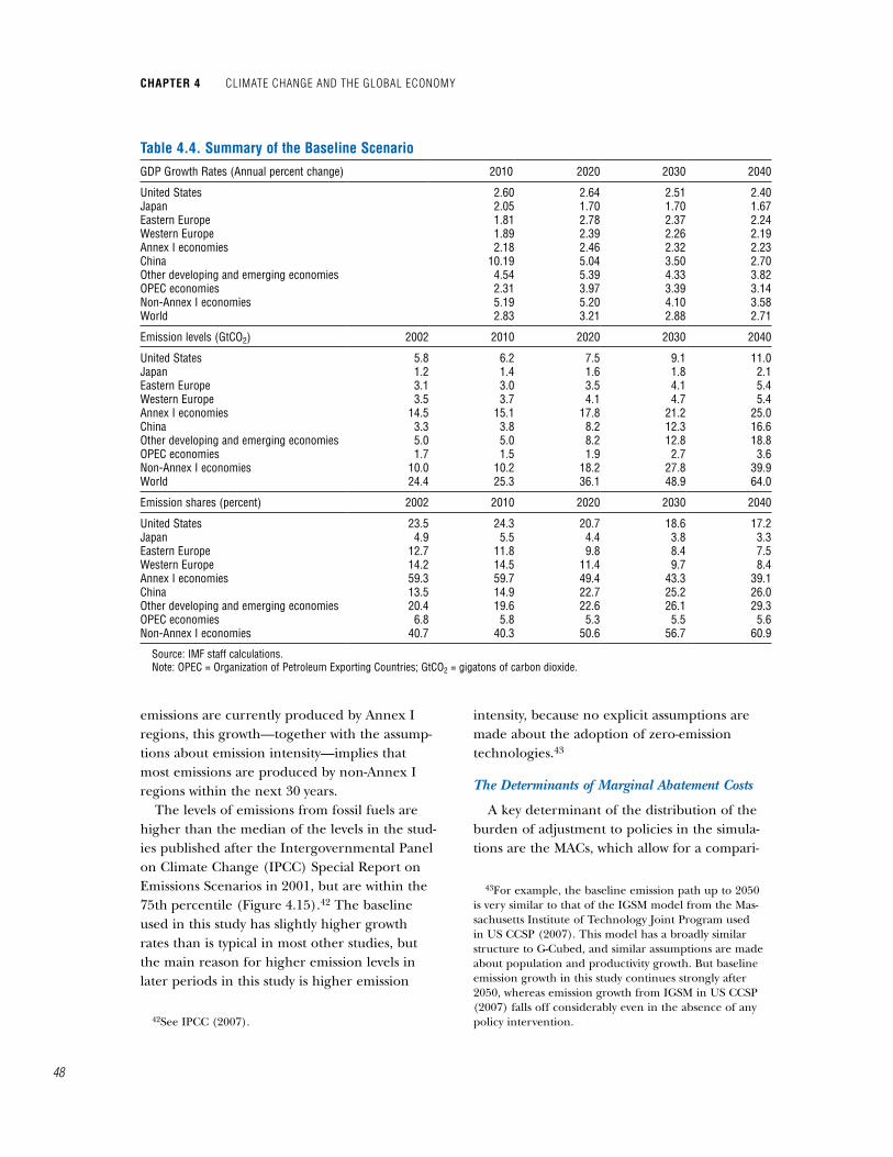
Chapter 4 Climate Change and the global eConomy
��
emissions are currently produced by Annex I regions, this growth—together with the assump-tions about emission intensity—implies that most emissions are produced by non-Annex I regions within the next �0 years.
The levels of emissions from fossil fuels are higher than the median of the levels in the stud-ies published after the Intergovernmental Panel on Climate Change (IPCC) Special Report on Emissions Scenarios in �00�, but are within the 7�th percentile (Figure �.��).�� The baseline used in this study has slightly higher growth rates than is typical in most other studies, but the main reason for higher emission levels in later periods in this study is higher emission
��See IPCC (�007).
intensity, because no explicit assumptions are made about the adoption of zero-emission technologies.��
The Determinants of Marginal Abatement Costs
A key determinant of the distribution of the burden of adjustment to policies in the simula-tions are the MACs, which allow for a compari-
��For example, the baseline emission path up to �0�0 is very similar to that of the IGSM model from the Mas-sachusetts Institute of Technology Joint Program used in US CCSP (�007). This model has a broadly similar structure to G-Cubed, and similar assumptions are made about population and productivity growth. But baseline emission growth in this study continues strongly after �0�0, whereas emission growth from IGSM in US CCSP (�007) falls off considerably even in the absence of any policy intervention.
table 4.4. Summary of the baseline ScenarioGDP Growth Rates (Annual percent change) 2010 2020 2030 2040
United States 2.60 2.64 2.51 2.40Japan 2.05 1.70 1.70 1.67Eastern Europe 1.81 2.78 2.37 2.24Western Europe 1.89 2.39 2.26 2.19Annex I economies 2.18 2.46 2.32 2.23China 10.19 5.04 3.50 2.70Other developing and emerging economies 4.54 5.39 4.33 3.82OPEC economies 2.31 3.97 3.39 3.14Non-Annex I economies 5.19 5.20 4.10 3.58World 2.83 3.21 2.88 2.71
Emission levels (GtCO2) 2002 2010 2020 2030 2040
United States 5.8 6.2 7.5 9.1 11.0Japan 1.2 1.4 1.6 1.8 2.1Eastern Europe 3.1 3.0 3.5 4.1 5.4Western Europe 3.5 3.7 4.1 4.7 5.4Annex I economies 14.5 15.1 17.8 21.2 25.0China 3.3 3.8 8.2 12.3 16.6Other developing and emerging economies 5.0 5.0 8.2 12.8 18.8OPEC economies 1.7 1.5 1.9 2.7 3.6Non-Annex I economies 10.0 10.2 18.2 27.8 39.9World 24.4 25.3 36.1 48.9 64.0
Emission shares (percent) 2002 2010 2020 2030 2040
United States 23.5 24.3 20.7 18.6 17.2Japan 4.9 5.5 4.4 3.8 3.3Eastern Europe 12.7 11.8 9.8 8.4 7.5Western Europe 14.2 14.5 11.4 9.7 8.4Annex I economies 59.3 59.7 49.4 43.3 39.1China 13.5 14.9 22.7 25.2 26.0Other developing and emerging economies 20.4 19.6 22.6 26.1 29.3OPEC economies 6.8 5.8 5.3 5.5 5.6Non-Annex I economies 40.7 40.3 50.6 56.7 60.9
Source: IMF staff calculations. Note: OPEC = Organization of Petroleum Exporting Countries; GtCO2 = gigatons of carbon dioxide.
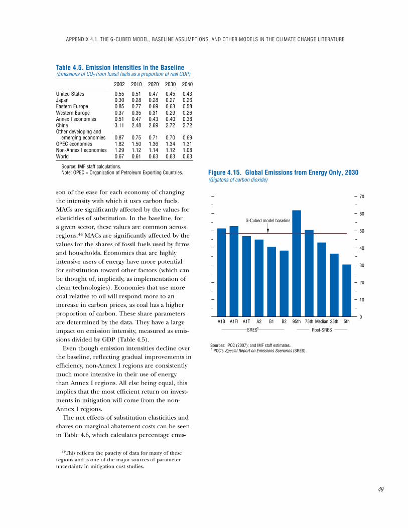
��
son of the ease for each economy of changing the intensity with which it uses carbon fuels. MACs are significantly affected by the values for elasticities of substitution. In the baseline, for a given sector, these values are common across regions.�� MACs are significantly affected by the values for the shares of fossil fuels used by firms and households. Economies that are highly intensive users of energy have more potential for substitution toward other factors (which can be thought of, implicitly, as implementation of clean technologies). Economies that use more coal relative to oil will respond more to an increase in carbon prices, as coal has a higher proportion of carbon. These share parameters are determined by the data. They have a large impact on emission intensity, measured as emis-sions divided by GDP (Table �.�).
Even though emission intensities decline over the baseline, reflecting gradual improvements in efficiency, non-Annex I regions are consistently much more intensive in their use of energy than Annex I regions. All else being equal, this implies that the most efficient return on invest-ments in mitigation will come from the non-Annex I regions.
The net effects of substitution elasticities and shares on marginal abatement costs can be seen in Table �.�, which calculates percentage emis-
��This reflects the paucity of data for many of these regions and is one of the major sources of parameter uncertainty in mitigation cost studies.
table 4.5. emission intensities in the baseline(Emissions of CO2 from fossil fuels as a proportion of real GDP)
2002 2010 2020 2030 2040
United States 0.55 0.51 0.47 0.45 0.43Japan 0.30 0.28 0.28 0.27 0.26Eastern Europe 0.85 0.77 0.69 0.63 0.58Western Europe 0.37 0.35 0.31 0.29 0.26Annex I economies 0.51 0.47 0.43 0.40 0.38China 3.11 2.48 2.69 2.72 2.72Other developing and
emerging economies 0.87 0.75 0.71 0.70 0.69OPEC economies 1.82 1.50 1.36 1.34 1.31Non-Annex I economies 1.29 1.12 1.14 1.12 1.08World 0.67 0.61 0.63 0.63 0.63
Source: IMF staff calculations.Note: OPEC = Organization of Petroleum Exporting Countries.
A1B A1FI A1T A2 B1 B2 95th 75th Median 25th 5th0
10
20
30
40
50
60
70
Figure 4.15. Global Emissions from Energy Only, 2030(Gigatons of carbon dioxide)
Sources: IPCC (2007); and IMF staff estimates. IPCC’s Special Report on Emissions Scenarios (SRES).
Post-SRES
G-Cubed model baseline
1
SRES1
appendix 4.1. the g-Cubed model, baseline assumptions, and other models in the Climate Change literature

Chapter 4 Climate Change and the global eConomy
�0
sion reductions and consumption losses from the baseline following a standardized carbon price increase of $�0 per ton of carbon.
The table shows that Japan achieves the low-est emission reduction of all economies when it raises carbon prices by the same amount. It has the highest MAC, which implies that it will reduce emissions less than all other regions when faced with a common carbon price, or will find it advantageous to buy emission rights under a cap-and-trade system. On the other hand, China can achieve approximately seven times the emission reduction as Japan for the same cost.��
For the world economy, G-Cubed has the same or lower abatement costs compared with other models. The main reason is that it explicitly models capital flows, which makes it easier for economies to install new capital and shift away from carbon-based energy in production.��
Comparisons with Other Models
The range of issues implied by climate change economics is reflected in the wide range
��In the experiment where a uniform carbon tax is imposed on all countries, this ratio increases to nearly 9:�, which illustrates the importance of reductions in export demand.
��The model is solved using linearization methods commonly applied to dynamic macroeconomic models. Linearization implies that responses of endogenous variables are proportional to the shock—a doubling of an increase in carbon taxes produces twice the reduction in emissions, for example. In practice, it may be that there are important nonlinearities in making the transition from old to new energy technologies.
of models, each of which emphasizes different aspects of the problem. In general, all these models aim to bring climate change analysis into a macroeconomic framework. But they differ substantially in the complexity with which they model the macroeconomy, climate, and technologies.
To illustrate the range of differences, Table �.7 summarizes features of some promi-nent models in the climate change literature:�7
• PAGE, maintained by Chris Hope and Cam-bridge University and used for the Stern Review simulations (Plambeck, Hope, and Anderson, �997);
• DICE, maintained by William Nordhaus at Yale and used in Nordhaus (�007b);
• EPPA/IGSM, maintained by a team at the Massachusetts Institute of Technology (Paltsev and others, �00�);
• MERGE, maintained by a team at Stanford University (Manne, Mendelsohn, and Richels, �99�); and
• MiniCAM, maintained by a team at Pacific Northwest National Laboratories (Brenkert and others, �00�).All of these models can claim some com-
parative advantage, usually because of more elaborate modeling of a particular sector or mechanism. Some of the main differences include the following:• whether behavior is optimizing and/or for-
ward looking (which can affect the effective-ness of carbon price increases);
�7The latter three were used in US CCSP (�007).
table 4.6. emission reductions and Consumption losses Following a Standardized Carbon price Shock(Percent deviations from baseline path)
UnitedStates Japan
WesternEurope
Eastern Europe and Russia China
Other Developingand Emerging Economies
Organizationof Petroleum
Exporting Countries
Emission reductionRank
8.007.00
2.101.00
2.302.00
2.403.00
15.00 9.00
3.004.00
9.008.00
Consumption lossRank
0.223.00
0.121.00
0.192.00
0.335.00
0.50 8.00
0.254.00
2.009.00
Source: IMF staff calculations. Note: Reduction in emissions and consumption losses measured at 2040, following a permanent unanticipated increase of $10 a ton of
carbon beginning in 2013 for each region, leaving all other regions’ carbon prices unchanged.
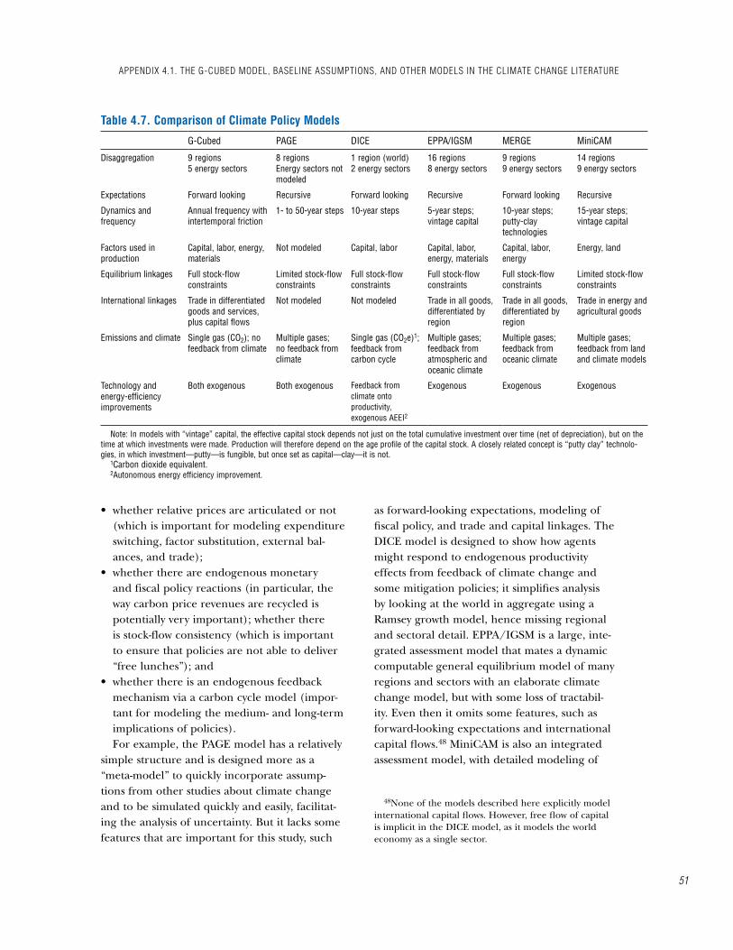
��
• whether relative prices are articulated or not (which is important for modeling expenditure switching, factor substitution, external bal-ances, and trade);
• whether there are endogenous monetary and fiscal policy reactions (in particular, the way carbon price revenues are recycled is potentially very important); whether there is stock-flow consistency (which is important to ensure that policies are not able to deliver “free lunches”); and
• whether there is an endogenous feedback mechanism via a carbon cycle model (impor-tant for modeling the medium- and long-term implications of policies).For example, the PAGE model has a relatively
simple structure and is designed more as a “meta-model” to quickly incorporate assump-tions from other studies about climate change and to be simulated quickly and easily, facilitat-ing the analysis of uncertainty. But it lacks some features that are important for this study, such
as forward-looking expectations, modeling of fiscal policy, and trade and capital linkages. The DICE model is designed to show how agents might respond to endogenous productivity effects from feedback of climate change and some mitigation policies; it simplifies analysis by looking at the world in aggregate using a Ramsey growth model, hence missing regional and sectoral detail. EPPA/IGSM is a large, inte-grated assessment model that mates a dynamic computable general equilibrium model of many regions and sectors with an elaborate climate change model, but with some loss of tractabil-ity. Even then it omits some features, such as forward-looking expectations and international capital flows.�8 MiniCAM is also an integrated assessment model, with detailed modeling of
�8None of the models described here explicitly model international capital flows. However, free flow of capital is implicit in the DICE model, as it models the world economy as a single sector.
table 4.7. Comparison of Climate policy models
G-Cubed PAGE DICE EPPA/IGSM MERGE MiniCAM
Disaggregation 9 regions5 energy sectors
8 regionsEnergy sectors not modeled
1 region (world)2 energy sectors
16 regions8 energy sectors
9 regions9 energy sectors
14 regions9 energy sectors
Expectations Forward looking Recursive Forward looking Recursive Forward looking Recursive
Dynamics and frequency
Annual frequency with intertemporal friction
1- to 50-year steps 10-year steps 5-year steps;vintage capital
10-year steps; putty-clay technologies
15-year steps; vintage capital
Factors used in production
Capital, labor, energy, materials
Not modeled Capital, labor Capital, labor, energy, materials
Capital, labor, energy
Energy, land
Equilibrium linkages Full stock-flow constraints
Limited stock-flow constraints
Full stock-flow constraints
Full stock-flow constraints
Full stock-flow constraints
Limited stock-flow constraints
International linkages Trade in differentiated goods and services, plus capital flows
Not modeled Not modeled Trade in all goods, differentiated by region
Trade in all goods, differentiated by region
Trade in energy and agricultural goods
Emissions and climate Single gas (CO2); no feedback from climate
Multiple gases; no feedback from climate
Single gas (CO2e)1; feedback from carbon cycle
Multiple gases; feedback from atmospheric and oceanic climate
Multiple gases; feedback from oceanic climate
Multiple gases; feedback from land and climate models
Technology and energy-efficiency improvements
Both exogenous Both exogenous Feedback from climate onto productivity, exogenous AEEI2
Exogenous Exogenous Exogenous
Note: In models with “vintage” capital, the effective capital stock depends not just on the total cumulative investment over time (net of depreciation), but on the time at which investments were made. Production will therefore depend on the age profile of the capital stock. A closely related concept is “putty clay” technolo-gies, in which investment—putty—is fungible, but once set as capital—clay—it is not.
1Carbon dioxide equivalent.2Autonomous energy efficiency improvement.
appendix 4.1. the g-Cubed model, baseline assumptions, and other models in the Climate Change literature
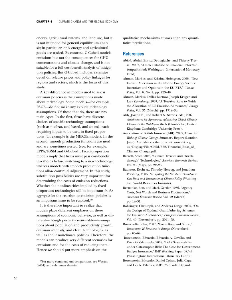
Chapter 4 Climate Change and the global eConomy
��
energy, agricultural systems, and land use, but it is not intended for general equilibrium analy-sis; in particular, only energy and agricultural goods are traded. By contrast, G-Cubed models emissions but not the consequences for GHG concentrations and climate change, and is not suitable for a full cost-benefit analysis of mitiga-tion policies. But G-Cubed includes extensive detail on relative prices and policy linkages for regions and sectors, which is the focus of this study.
A key difference in models used to assess emission policies is the assumptions made about technology. Some models—for example, PAGE—do not make any explicit technology assumptions. Of those that do, there are two main types. In the first, firms have discrete choices of specific technology assumptions (such as nuclear, coal-based, and so on), each requiring inputs to be used in fixed propor-tions (an example is the MERGE model). In the second, smooth production functions are used and are sometimes nested (see, for example, EPPA/IGSM and G-Cubed). Fixed-proportion models imply that firms must pass cost-benefit thresholds before switching to a new technology, whereas models with smooth production func-tions allow continual adjustment. In this study, substitution possibilities are very important for determining the costs of emission reductions. Whether the nonlinearities implied by fixed-proportion technologies will be important in the aggregate for the reaction to emission policies is an important issue to be resolved.�9
It is therefore important to realize that models place different emphases on these assumptions of economic behavior, as well as dif-ferent—though perfectly reasonable—assump-tions about population and productivity growth, emission intensity, and clean technologies, as well as about nonclimate policies. Therefore, the models can produce very different scenarios for emissions and for the costs of reducing them. Hence we should put more emphasis on the
�9For more comment and comparisons, see Weyant (�00�) and references therein.
qualitative mechanisms at work than any quanti-tative predictions.
referencesAbiad, Abdul, Enrica Detragiache, and Thierry Tres-
sel, �007, “A New Database of Financial Reforms” (unpublished; Washington: International Monetary Fund).
Åhman, Markus, and Kristina Holmgren, �00�, “New Entrant Allocation in the Nordic Energy Sectors: Incentives and Options in the EU ETS,” Climate Policy, Vol. �, No. �, pp. ���–�0.
Åhman, Markus, Dallas Burtraw, Joseph Kruger, and Lars Zetterberg, �007, “A Ten-Year Rule to Guide the Allocation of EU Emission Allowances,” Energy Policy, Vol. �� (March), pp. �7�8–�0.
Aldy, Joseph E., and Robert N. Stavins, eds., �007, Architectures for Agreement: Addressing Global Climate Change in the Post-Kyoto World (Cambridge, United Kingdom: Cambridge University Press).
Association of British Insurers (ABI), �00�, Financial Risks of Climate Change, Summary Report (London, June). Available via the Internet: www.abi.org.uk/Display/File/Child/���/Financial_Risks_of_ Climate_Change.pdf.
Barrett, Scott, �00�, “Climate Treaties and ‘Break-through’ Technologies,” American Economic Review, Vol. 9� (May), pp. ��–��.
Baumert, Kevin A., Timothy Herzog, and Jonathan Pershing, �00�, Navigating the Numbers: Greenhouse Gas Data and International Climate Policy (Washing-ton: World Resources Institute).
Bernanke, Ben, and Mark Gertler, �989, “Agency Costs, Net Worth and Business Fluctuations,” American Economic Review, Vol. 79 (March), pp. ��–��.
Böhringer, Christoph, and Andreas Lange, �00�, “On the Design of Optimal Grandfathering Schemes for Emission Allowances,” European Economic Review, Vol. �9 (November), pp. �0��–��.
Bonaccolta, John, �007, “Come Rain and Shine,” Investment & Pensions in Europe (November), pp. ��–��.
Borensztein, Eduardo, Eduardo A. Cavallo, and Patricio Valenzuela, �008, “Debt Sustainability under Catastrophic Risk: The Case for Government Budget Insurance,” IMF Working Paper 08/�� (Washington: International Monetary Fund).
Borensztein, Eduardo, Daniel Cohen, Julia Cage, and Cécile Valadier, �008, “Aid Volatility and
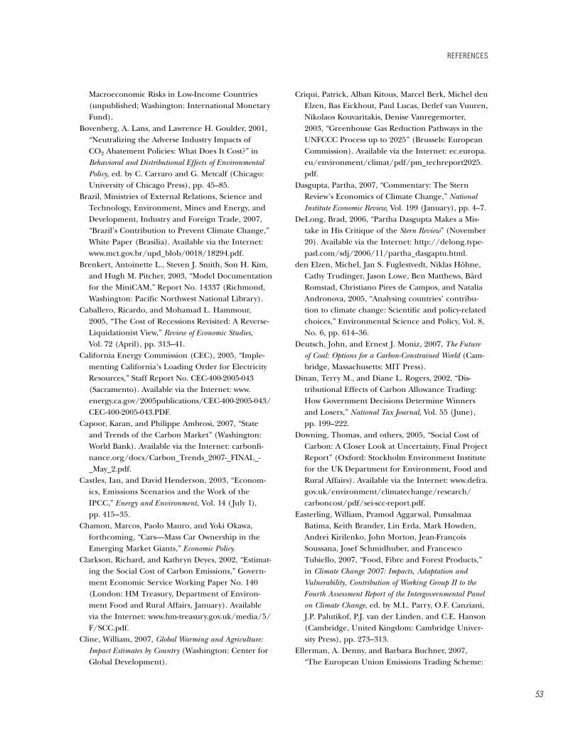
��
Macroeconomic Risks in Low-Income Countries (unpublished; Washington: International Monetary Fund).
Bovenberg, A. Lans, and Lawrence H. Goulder, �00�, “Neutralizing the Adverse Industry Impacts of CO� Abatement Policies: What Does It Cost?” in Behavioral and Distributional Effects of Environmental Policy, ed. by C. Carraro and G. Metcalf (Chicago: University of Chicago Press), pp. ��–8�.
Brazil, Ministries of External Relations, Science and Technology, Environment, Mines and Energy, and Development, Industry and Foreign Trade, �007, “Brazil’s Contribution to Prevent Climate Change,” White Paper (Brasilia). Available via the Internet: www.mct.gov.br/upd_blob/00�8/�8�9�.pdf.
Brenkert, Antoinette L., Steven J. Smith, Son H. Kim, and Hugh M. Pitcher, �00�, “Model Documentation for the MiniCAM,” Report No. ����7 (Richmond, Washington: Pacific Northwest National Library).
Caballero, Ricardo, and Mohamad L. Hammour, �00�, “The Cost of Recessions Revisited: A Reverse- Liquidationist View,” Review of Economic Studies, Vol. 7� (April), pp. ���–��.
California Energy Commission (CEC), �00�, “Imple-menting California’s Loading Order for Electricity Resources,” Staff Report No. CEC-�00-�00�-0�� (Sacramento). Available via the Internet: www.energy.ca.gov/�00�publications/CEC-�00-�00�-0��/ CEC-�00-�00�-0��.PDF.
Capoor, Karan, and Philippe Ambrosi, �007, “State and Trends of the Carbon Market” (Washington: World Bank). Available via the Internet: carbonfi-nance.org/docs/Carbon_Trends_�007-_FINAL_-_May_�.pdf.
Castles, Ian, and David Henderson, �00�, “Econom-ics, Emissions Scenarios and the Work of the IPCC,” Energy and Environment, Vol. �� (July �), pp. ���–��.
Chamon, Marcos, Paolo Mauro, and Yoki Okawa, forthcoming, “Cars—Mass Car Ownership in the Emerging Market Giants,” Economic Policy.
Clarkson, Richard, and Kathryn Deyes, �00�, “Estimat-ing the Social Cost of Carbon Emissions,” Govern-ment Economic Service Working Paper No. ��0 (London: HM Treasury, Department of Environ-ment Food and Rural Affairs, January). Available via the Internet: www.hm-treasury.gov.uk/media/�/F/SCC.pdf.
Cline, William, �007, Global Warming and Agriculture: Impact Estimates by Country (Washington: Center for Global Development).
Criqui, Patrick, Alban Kitous, Marcel Berk, Michel den Elzen, Bas Eickhout, Paul Lucas, Detlef van Vuuren, Nikolaos Kouvaritakis, Denise Vanregemorter, �00�, “Greenhouse Gas Reduction Pathways in the UNFCCC Process up to �0��” (Brussels: European Commission). Available via the Internet: ec.europa.eu/environment/climat/pdf/pm_techreport�0��.pdf.
Dasgupta, Partha, �007, “Commentary: The Stern Review’s Economics of Climate Change,” National Institute Economic Review, Vol. �99 (January), pp. �–7.
DeLong, Brad, �00�, “Partha Dasgupta Makes a Mis-take in His Critique of the Stern Review” (November �0). Available via the Internet: http://delong.type-pad.com/sdj/�00�/��/partha_dasgaptu.html.
den Elzen, Michel, Jan S. Fuglestvedt, Niklas Höhne, Cathy Trudinger, Jason Lowe, Ben Matthews, Bård Romstad, Christiano Pires de Campos, and Natalia Andronova, �00�, “Analysing countries’ contribu-tion to climate change: Scientific and policy-related choices,” Environmental Science and Policy, Vol. 8, No. �, pp. ���–��.
Deutsch, John, and Ernest J. Moniz, �007, The Future of Coal: Options for a Carbon-Constrained World (Cam-bridge, Massachusetts: MIT Press).
Dinan, Terry M., and Diane L. Rogers, �00�, “Dis-tributional Effects of Carbon Allowance Trading: How Government Decisions Determine Winners and Losers,” National Tax Journal, Vol. �� (June), pp. �99–���.
Downing, Thomas, and others, �00�, “Social Cost of Carbon: A Closer Look at Uncertainty, Final Project Report” (Oxford: Stockholm Environment Institute for the UK Department for Environment, Food and Rural Affairs). Available via the Internet: www.defra.gov.uk/environment/climatechange/research/carboncost/pdf/sei-scc-report.pdf.
Easterling, William, Pramod Aggarwal, Punsalmaa Batima, Keith Brander, Lin Erda, Mark Howden, Andrei Kirilenko, John Morton, Jean-François Soussana, Josef Schmidhuber, and Francesco Tubiello, �007, “Food, Fibre and Forest Products,” in Climate Change 2007: Impacts, Adaptation and Vulnerability, Contribution of Working Group II to the Fourth Assessment Report of the Intergovernmental Panel on Climate Change, ed. by M.L. Parry, O.F. Canziani, J.P. Palutikof, P.J. van der Linden, and C.E. Hanson (Cambridge, United Kingdom: Cambridge Univer-sity Press), pp. �7�–���.
Ellerman, A. Denny, and Barbara Buchner, �007, “The European Union Emissions Trading Scheme:
referenCes
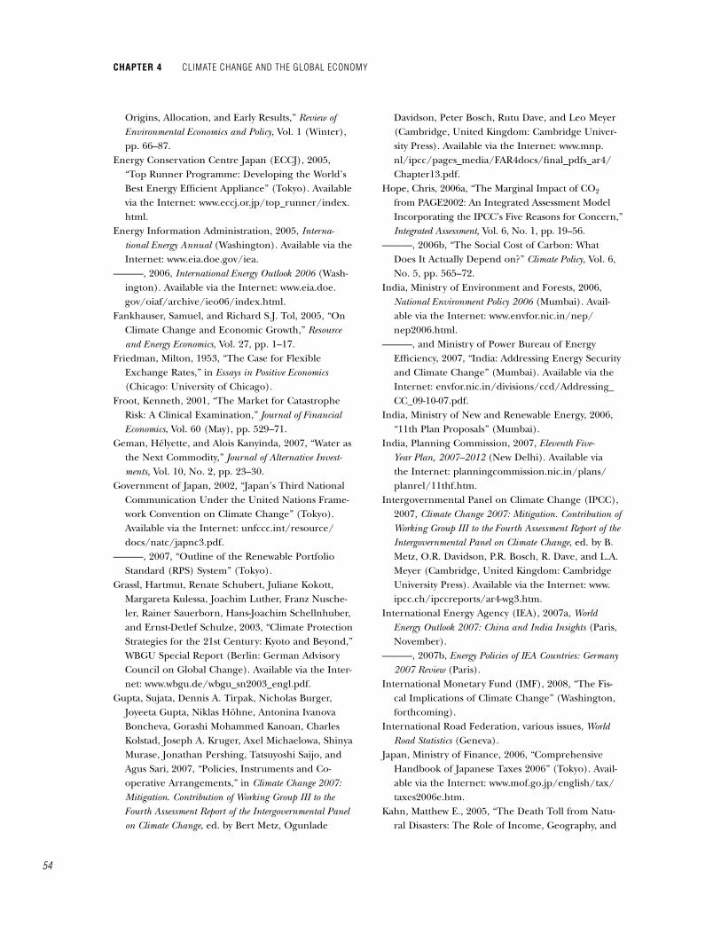
Chapter 4 Climate Change and the global eConomy
��
Origins, Allocation, and Early Results,” Review of Environmental Economics and Policy, Vol. � (Winter), pp. ��–87.
Energy Conservation Centre Japan (ECCJ), �00�, “Top Runner Programme: Developing the World’s Best Energy Efficient Appliance” (Tokyo). Available via the Internet: www.eccj.or.jp/top_runner/index.html.
Energy Information Administration, �00�, Interna-tional Energy Annual (Washington). Available via the Internet: www.eia.doe.gov/iea.
———, �00�, International Energy Outlook 2006 (Wash-ington). Available via the Internet: www.eia.doe.gov/oiaf/archive/ieo0�/index.html.
Fankhauser, Samuel, and Richard S.J. Tol, �00�, “On Climate Change and Economic Growth,” Resource and Energy Economics, Vol. �7, pp. �–�7.
Friedman, Milton, �9��, “The Case for Flexible Exchange Rates,” in Essays in Positive Economics (Chicago: University of Chicago).
Froot, Kenneth, �00�, “The Market for Catastrophe Risk: A Clinical Examination,” Journal of Financial Economics, Vol. �0 (May), pp. ��9–7�.
Geman, Hélyette, and Alois Kanyinda, �007, “Water as the Next Commodity,” Journal of Alternative Invest-ments, Vol. �0, No. �, pp. ��–�0.
Government of Japan, �00�, “Japan’s Third National Communication Under the United Nations Frame-work Convention on Climate Change” (Tokyo). Available via the Internet: unfccc.int/resource/docs/natc/japnc�.pdf.
———, �007, “Outline of the Renewable Portfolio Standard (RPS) System” (Tokyo).
Grassl, Hartmut, Renate Schubert, Juliane Kokott, Margareta Kulessa, Joachim Luther, Franz Nusche-ler, Rainer Sauerborn, Hans-Joachim Schellnhuber, and Ernst-Detlef Schulze, �00�, “Climate Protection Strategies for the ��st Century: Kyoto and Beyond,” WBGU Special Report (Berlin: German Advisory Council on Global Change). Available via the Inter-net: www.wbgu.de/wbgu_sn�00�_engl.pdf.
Gupta, Sujata, Dennis A. Tirpak, Nicholas Burger, Joyeeta Gupta, Niklas Höhne, Antonina Ivanova Boncheva, Gorashi Mohammed Kanoan, Charles Kolstad, Joseph A. Kruger, Axel Michaelowa, Shinya Murase, Jonathan Pershing, Tatsuyoshi Saijo, and Agus Sari, �007, “Policies, Instruments and Co-operative Arrangements,” in Climate Change 2007: Mitigation. Contribution of Working Group III to the Fourth Assessment Report of the Intergovernmental Panel on Climate Change, ed. by Bert Metz, Ogunlade
Davidson, Peter Bosch, Rutu Dave, and Leo Meyer (Cambridge, United Kingdom: Cambridge Univer-sity Press). Available via the Internet: www.mnp.nl/ipcc/pages_media/FAR�docs/final_pdfs_ar�/Chapter��.pdf.
Hope, Chris, �00�a, “The Marginal Impact of CO� from PAGE�00�: An Integrated Assessment Model Incorporating the IPCC’s Five Reasons for Concern,” Integrated Assessment, Vol. �, No. �, pp. �9–��.
———, �00�b, “The Social Cost of Carbon: What Does It Actually Depend on?” Climate Policy, Vol. �, No. �, pp. ���–7�.
India, Ministry of Environment and Forests, �00�, National Environment Policy 2006 (Mumbai). Avail-able via the Internet: www.envfor.nic.in/nep/nep�00�.html.
———, and Ministry of Power Bureau of Energy Efficiency, �007, “India: Addressing Energy Security and Climate Change” (Mumbai). Available via the Internet: envfor.nic.in/divisions/ccd/Addressing_ CC_09-�0-07.pdf.
India, Ministry of New and Renewable Energy, �00�, “��th Plan Proposals” (Mumbai).
India, Planning Commission, �007, Eleventh Five-Year Plan, 2007–2012 (New Delhi). Available via the Internet: planningcommission.nic.in/plans/planrel/��thf.htm.
Intergovernmental Panel on Climate Change (IPCC), �007, Climate Change 2007: Mitigation. Contribution of Working Group III to the Fourth Assessment Report of the Intergovernmental Panel on Climate Change, ed. by B. Metz, O.R. Davidson, P.R. Bosch, R. Dave, and L.A. Meyer (Cambridge, United Kingdom: Cambridge University Press). Available via the Internet: www.ipcc.ch/ipccreports/ar�-wg�.htm.
International Energy Agency (IEA), �007a, World Energy Outlook 2007: China and India Insights (Paris, November).
———, �007b, Energy Policies of IEA Countries: Germany 2007 Review (Paris).
International Monetary Fund (IMF), �008, “The Fis-cal Implications of Climate Change” (Washington, forthcoming).
International Road Federation, various issues, World Road Statistics (Geneva).
Japan, Ministry of Finance, �00�, “Comprehensive Handbook of Japanese Taxes �00�” (Tokyo). Avail-able via the Internet: www.mof.go.jp/english/tax/taxes�00�e.htm.
Kahn, Matthew E., �00�, “The Death Toll from Natu-ral Disasters: The Role of Income, Geography, and
��
Institutions,” Review of Economics and Statistics, Vol. 87 (May), pp. �7�–8�.
Kiyotaki, Nobuhiro, and John Moore, �997, “Credit Cycles,” Journal of Political Economy, Vol. �0� (April), pp. ���–�8.
Kopp, Raymond, Richard Morgenstern, and William Pizer, �997. “Something for Everyone: A Climate Policy that Both Environmentalists and Industry Can Live With” (Washington: Resources for the Future). Available via the Internet: www.weather-vane.rff.org/SomethingForEveryone.pdf.
Kopp, Raymond J., and William A. Pizer, eds., �007, Assessing U.S. Climate Policy Options (Washington: Resources for the Future). Available via the Inter-net: www.rff.org/rff/Publications/CPF_Assessin-gUSClimatePolicyOptions.cfm.
Kumhof, Michael, and Douglas Laxton, �007, “A Party Without a Hangover? On the Effects of U.S. Government Deficits,” IMF Working Paper 07/�0� (Washington: International Monetary Fund).
Ligthart, Jenny, and Rosa Martín Suárez, �00�, “The Productivity of Public Capital: A Meta Analysis,” (unpublished; Tilburg, Netherlands: Tilburg University). Available via the Internet: center.uvt.nl/staff/ligthart/meta.pdf.
Manne, Alan S., Robert Mendelsohn, and Richard G. Richels, �99�, “MERGE—A Model for Evaluat-ing Regional and Global Effects of GHG Reduc-tion Policies,” Energy Policy, Vol. �� (January), pp. �7–��.
Matsuyama, Kiminori, �007, “Aggregate Implications of Credit Market Imperfections,” NBER Work-ing Paper No. ���09 (Cambridge, Massachusetts: National Bureau of Economic Research).
McKibbin, Warwick J., and Peter J. Wilcoxen, �997, “A Better Way to Slow Global Climate Change,” Policy Brief No. �7 (Washington: The Brookings Institution).
———, �998, “The Theoretical and Empirical Struc-ture of the G-Cubed Model” Economic Modelling, Vol. �� (January �), pp. ���–�8.
———, �00�a, “An Alternative to Kyoto?” New Economy, Vol. 9 (September), pp. ���–�8.
———, �00�b, Climate Change Policy After Kyoto: A Blue-print for a Realistic Approach (Washington: Brookings Institution Press).
———, �00�c, “The Role of Economics in Climate Change Policy,” Journal of Economic Perspectives, Vol. �� (Spring), pp. �07–�9.
———, �00�, “Estimates of the Costs of Kyoto-Mar-rakesh Versus the McKibbin-Wilcoxen Blueprint,” Energy Policy, Vol. �� (March), pp. ��7–79.
Mendelsohn, Robert, Michael Schlesinger, and Larry Williams, �000, “Comparing Impacts Across Climate Models,” Integrated Assessment, Vol. � (March), pp. �7–�8.
Metcalf, Gilbert E., �007, “A Proposal for a U.S. Car-bon Tax Swap: An Equitable Tax Reform to Address Global Climate Change,” Hamilton Project Discus-sion Paper No. �007-�� (Washington: The Brook-ings Institution). Available via the Internet: www.brookings.edu/~/media/Files/rc/papers/�007/�0carbontax_metcalf/�0_carbontax_metcalf.pdf.
Meyers, Stephen, James McMahon, Michael McNeil, and Xiaomin Liu, �00�, “Realized and Prospective Impacts of U.S. Energy Efficiency Standards for Residential Appliances,” Report No. LBNL-�9�0� (Berkeley, California: Lawrence Berkeley National Laboratory).
Miguel, Edward, Shanker Satyanath, and Ernest Ser-genti, �00�, “Economic Shocks and Civil Conflict: An Instrumental Variables Approach,” Journal of Political Economy, Vol. ��� (August), pp. 7��–��.
Mundell, Robert A., �9��, “A Theory of Optimum Currency Areas,” American Economic Review, Vol. �� (September), pp. ��7–��.
Nakicenovic, Nebosja, and Keywan Riahi, �00�, “Model Runs with MESSAGE in the Context of the Further Development of the Kyoto Protocol,” Expertise for the WBGU Special Report “Climate Protection Strategies for the ��st Century: Kyoto and Beyond” (Berlin). Available via the Internet: www.wbgu.de/wbgu_sn�00�_ex0�.pdf.
Nordhaus, William D., �007a, “A Review of the Stern Review of the Economics of Climate Change,” Jour-nal of Economic Literature, Vol. �� (September), pp. �8�–70�.
———, �007b, “The Challenge of Global Warm-ing: Economic Models and Environmental Policy” (unpublished). Available via the Internet: nordhaus.econ.yale.edu/dice_mss_09��07_public.pdf.
———, �007c, “Alternative Measures of Output in Global Economic-Environmental Models: Purchas-ing Power Parity or Market Exchange Rates?” Energy Economics, Vol. �9 (May), pp. ��9–7�.
———, and Joseph Boyer, �000, Warming the World: Economic Models of Global Warming (Cambridge, Massachusetts: MIT Press).
Nordqvist, Joakim, �00�, “Evaluation of Japan’s Top Runner Programme Within the Framework of the AID-EE Project,” Active Implementation of the European Directive on Energy Efficiency. Avail-
referenCes

Chapter 4 Climate Change and the global eConomy
��
able via the Internet: www.aid-ee.org/documents/0�8TopRunner-Japan.pdf.
Obstfeld, Maurice, and K. Rogoff, �00�, Foundations of International Macroeconomics, Fifth Edition (Cam-bridge, Massachusetts: MIT Press).
Olivier, Jos, and Jan Berdowski, �00�, “Global Emis-sion Sources and Sinks,” in The Climate System, ed. by Jan Berdowski, Robert Guicherit, and BertJan Heij (Lisse, Netherlands: Swets & Zeitlinger B.V.), pp. ��–78.
Paltsev, Sergey, John M. Reilly, Henry D. Jacoby, Richard S. Eckaus, James McFarland, Marcus Sarofim, Malcolm Asadoorian, and Mustafa Babiker, �00�, “The MIT Emissions Prediction and Policy Analysis (EPPA) Model: Version �,” Report No. ��� (Cambridge, Massachusetts: Massachusetts Institute of Technology, Joint Program on the Science and Policy of Global Change).
Parry, Ian W.H., Roberton C. Williams, III, and Lawrence H. Goulder, �999, “When Can Carbon Abatement Policies Increase Welfare? The Funda-mental Role of Distorted Factor Markets,” Journal of Environmental Economics and Management, Vol. �7 (January), pp. ��–8�.
Persson, Tobias, Christian Azar, and Kristian Lind-gren, �00�, “Allocation of CO� Emission Permits—Economic Incentives for Emissions Reductions in Developing Countries,” Energy Policy, Vol. �� (September), pp. �889–99.
Pindyck, Robert S., �007, “Uncertainty in Environmen-tal Economics,” Review of Environmental Economics and Policy, Vol. �, No. �, pp. ��–��.
Pizer, William A., �00�, “Combining Price and Quan-tity Controls to Mitigate Global Climate Change,” Journal of Public Economics, Vol. 8� (September), pp. �09–��.
Plambeck, Erica L., Chris Hope, and John Anderson, �997, “The [PAGE9�] Model: Integrating the Sci-ence and Economics of Global Warming,” Energy Economics, Vol. �9 (March), pp. 77–�0�.
Point Carbon Research, �008, “A Review of �007,” Carbon Market Monitor (January).
Ramcharan, Rodney, �007a, “Does the Exchange Rate Regime Matter for Real Shocks? Evidence from Windstorms and Earthquakes,” Journal of Interna-tional Economics, Vol. 7� (September), pp. ��–�7.
———, �007b, “Floods, Windstorms, and the Finan-cial System” (unpublished; Washington: Interna-tional Monetary Fund).
Rosendahl, Knut Einar, �007, “Incentives and Quota Prices in an Emission Trading Scheme with
Updating,” Research Department Working Paper No. �9� (Oslo: Statistics Norway). Available via the Internet: www.ssb.no/publikasjoner/DP/pdf/dp�9�.pdf.
Sedjo, Roger A., and Michael Toman, �00�, “Can Carbon Sinks Be Operational? RFF Workshop Proceedings,” Discussion Paper No. 0�–�� (Washington: Resources for the Future). Available via the Internet: www.rff.org/rff/Documents/ RFF-DP-0�-��.pdf.
Stavins, Robert N., and Kenneth R. Richards, �00�, “The Cost of U.S. Forest-Based Carbon Sequestra-tion” (Arlington, Virginia: Pew Center on Global Climate Change). Available via the Internet: http://www.pewclimate.org/docUploads/Sequest_Final.pdf.
Stern, Nicholas, �008, “The Economics of Climate Change,” Richard T. Ely Lecture, American Eco-nomic Association Meetings, New Orleans, Louisi-ana (January �).
Stern, Nicholas, and others, �007, The Economics of Climate Change: The Stern Review (London: HM Treasury).
Strand, Jon, �007, “Energy Efficiency and Renewable Energy Supply for the G-7 Countries, with Emphasis on Germany,” IMF Working Paper 07/�99 (Wash-ington: International Monetary Fund).
Stromberg, David, �007, “Natural Disasters, Economic Development, and Humanitarian Aid,” Journal of Economic Perspectives, Vol. �� (Summer), pp. �99–���.
Tol, Richard S.J., �00�, “Estimates of the Damage Costs of Climate Change. Part �: Benchmark Esti-mates,” Environmental and Resource Economics, Vol. �� (January), pp. �7–7�.
———, �00�, “The Marginal Damage Costs of Carbon Dioxide Emissions: An Assessment of the Uncertainties,” Energy Policy, Vol. �� (November), pp. �0��–7�.
United Kingdom Climate Impacts Programme (UKCIP), �007, UKCIP Climate Digest: April 2007 (Oxford). Available via the Internet: www. ukcip.org.uk/news_releases/�8.pdf.
United Nations, �998, “Kyoto Protocol to the United Nations Framework Convention on Climate Change” (New York). Available via the Internet: unfccc.int/resource/docs/convkp/kpeng.pdf.
———, �00�, “World Population Prospects: The �00� Revision Population Database” (New York). Avail-able via the Internet: esa.un.org/unpp.
United Nations Development Program (UNDP), �007, Human Development Report 2007/2008, Fighting
��
Climate Change: Human Solidarity in a Divided World (New York).
United Nations Framework Convention on Climate Change (UNFCCC), �007, Investment and Financial Flows to Address Climate Change (Bonn).
U.S. Climate Change Science Program (US CCSP), �007, Scenarios of Greenhouse Gas Emissions and Atmospheric Concentrations and Review of Integrated Scenario Development and Application, Synthesis and Assessment Product �.� (Washington: Depart-ment of Energy). Available via the Internet: www.climatescience.gov/Library/sap/sap�-�/default.php.
van Aardenne, J.A., F.J. Dentener, J.G.J. Olivier, C.G.M. Klein Goldewijk, and J. Lelieveld, �00�, “A � Degree x � Degree Resolution Dataset of Historical Anthropogenic Trace Gas Emissions for the Period �890–�990,” Global Biogeochemical Cycles, Vol. ��, No. �, pp. 909–�8.
van Lennep, David, Teddy Oetomo, Maxwell Stevenson, and André de Vries, �00�, “Weather Derivatives: An Attractive Additional Asset Class,” Journal of Alternative Investments, Vol. 7 (Fall), pp. ��–7�.
Wasmer, Etienne, and Philippe Weil, �00�, “The Macroeconomics of Labor and Credit Market Imperfections,” American Economic Review, Vol. 9� (September), pp. 9��–��.
Webster, Mort, Chris Forest, John Reilly, Mustafa Babiker, David Kicklighter, Monika Mayer, Ron-ald Prinn, Marcus Sarofim, Andrei Sokolov, Peter Stone, and Chien Wang, �00�, “Uncertainty Analysis of Climate Change and Policy Response,” Climatic Change, Vol. ��, No. �, pp. �9�–��0.
Weitzman, Martin, �007a, “The Role of Uncertainty in the Economics of Catastrophic Climate Change,” Working Paper 07-�� (Washington: AEI-Brookings Joint Center).
———, �007b, “A Review of the Stern Review of the Economics of Climate Change,” Journal of Economic Literature, Vol. �� (September), pp. 70�–��.
———, �008, “On Modeling and Interpreting the Economics of Catastrophic Climate Change” (unpublished). Available via the Internet: www.economics.harvard.edu/faculty/weitzman/files/modeling.pdf.
Weyant, John P., �00�, “Introduction and Overview,” Energy Economics, Vol. ��, “EMF �9 Alternative Tech-nology Strategies for Climate Change Policy” (July), pp. �0�–��.
World Bank, �00�, Clean Energy and Development: Towards an Investment Framework (Washington).
Wright, Brian D., �98�, “The Economics of Invention Incentives: Patents, Prizes and Research Contracts,” American Economic Review, Vol. 7� (September), pp. �9�–707.
Yohe, Gary, Rodel Lasco, Qazi Ahmad, Nigel Arnell, Stewart Cohen, Chris Hope, Anthony Janetos, and Rosa Perez, �007, “Perspectives on Climate Change and Sustainability,” in Climate Change 2007: Impacts, Adaptation, and Vulnerability. Contributions of Working Group II to the Fourth Assessment Report of the Inter-governmental Panel on Climate Change, ed. by Martin Parry, Osvaldo Canziani, Jean Palutikof, Paul van der Linden, and Clair E. Hanson (Cambridge, United Kingdom: Cambridge University Press), pp. 8��–��. Available via the Internet: www.ipcc.ch/pdf/assess-ment-report/ar�/wg�/ar�-wg�-chapter�0.pdf.
referenCes