Click on the desired section below to position to that page. You may

Click on the desired section below to position to that page. You may also scroll to browse the document. Supplemental Topic 2: Nonparametric Tests of Hypotheses S2.1 Sign Test S2.2 The Two-Sample Rank Sum Test S2.3 Wilcoxon Signed-Rank Test S2.4 Kruskal-Wallis Test Exercises

S2-1

SUPPLEMENTALTOPIC 2

Will the highest ranked wines come from here?See Example S2.6 (p. S2-17)

Ian

Shaw

/Sto

ne/G

etty

Imag

es

S2-W3527 9/28/05 4:03 PM Page S2-1

Chapter Title

Chapter opeing quote (8pts b/r to box end, 36pts to ch op text)

S2-2

A distinguishing feature of a nonparametric test is that it can beused without having to assume a specific type of distribution forthe measurements in the population(s) being studied. The validity

of a nonparametric method, for instance, does not depend on the assump-tion that the response variable has a normal distribution, as is the casefor the t-test procedures described in Sections 13.2, 13.3, and 13.4 for test-ing hypotheses about either one or two population means. Thus, almostby definition, nonparametric methods are robust, which means that theyare valid over a broad range of circumstances.

Most nonparametric tests are based on simple counting and rankingprocedures. As an example, suppose that we want to know whether themedian amount spent on textbooks last year by students at a universitywas $700 (a null value) or more than $700 (an alternative hypothesis). Wecould simply count how many students in a random sample spent morethan $700. If the population median actually was $700, then by the defini-tion of a median, roughly half of the sample would have spent more than$700 (and the other half would have spent less). If “significantly” morethan half of the sample spent over $700, it would be evidence that thepopulation median was greater than $700. We’ll learn how to determine ap-value for this type of situation in Section S2.1, where we describe thesign test. An important point to note is that the procedure we use to findthe p-value is appropriate for any continuous random variable, not justnormal random variables.

Generally, nonparametric procedures are resistant to the influence ofoutliers. The number of students who spent over $700 will not be undulyinfluenced by outliers. Somebody who had the misfortune to have spent$2,000 is merely counted as a student who spent more than $700, just assomebody who spent $750 would be. Because the test statistic (how manyspent over $700) does not use the specific amounts, it is resistant to theinfluence of outliers.

Nonparametric Tests of Hypotheses

Most nonparametric tests are based on simple counting and ranking procedures. Gener-ally, nonparametric procedures are resistant to the influence of outliers and are robust,which means that they are valid over a broad range of circumstances.

Throughout the chapter, this icon introduces a list of resources on theStatisticsNow website at http://1pass.thomson.com that will:• Help you evaluate your knowledge

of the material• Allow you to take an exam-

prep quiz• Provide a Personalized Learning

Plan targeting resources thataddress areas you should study

S2-W3527 9/28/05 4:03 PM Page S2-2

The term nonparametric test originated because the test statistic insuch a test does not depend on sample estimate(s) of parameter(s) in apopulation distribution. In contrast, recall the one-sample t-test proce-dure described in Section 13.2 for testing hypotheses about a populationmean. The one-sample t-test is a parametric test. The t-statistic involves

and s, the sample mean and sample standard deviation. These are esti-mates of the parameters m and s, the mean and standard deviation of thepopulation distribution, which is assumed to be a normal curve in theone-sample t-test problem. ❚

S2.1 The Sign TestThe sign test can be used to test hypotheses about the population median whenthe response is a continuous variable. (Recall from Chapter 8 that a continuousrandom variable is one for which any value within some interval is a possibleoutcome.) We will use the symbol h (“eta”) to represent the population median.Thus, the null hypothesis for a sign test could be written as

H0: h� h0 (population median equals a specified value)

The alternative hypothesis can be one-sided (either Ha: h� h0 or Ha: h� h0) ortwo-sided (Ha: h � h0). When the alternative hypothesis is one-sided, the nullhypothesis can be written to include an inequality in the opposite direction.

If the response of interest is a discrete random variable (a variable with acountable set of possible outcomes), the hypotheses must be written differ-ently, particularly when the number of possible outcomes is small. We willcover that situation later in this section. For now, we assume that the responsevariable is continuous. In that case, we are using the sign test to test hypothesesabout the value of the population median.

As an example, we could use the sign test to test whether the medianamount spent on textbooks last year at a university was $700 (or less) or morethan $700. The null and alternative hypotheses in this situation are

H0: h� 700 (population median equals 700)

Ha: h� 700 (population median is greater than 700)

The null hypothesis could also be written as H0: h� 700.Most commonly, the sign test is used to analyze paired data, and this appli-

cation gives the test its name. The usual null hypothesis for the difference be-tween the paired measurements is that the median difference is 0 (H0: h � 0).Suppose, for example, that a sample of college men reports their actual anddesired weights. For each man, we could find difference � actual � desired, thedifference between the two responses. This difference will be greater than 0(positive) when a man wants to lose weight; it will be less than 0 (negative) whena man wants to gain weight. To consider the null hypothesis that the populationmedian difference is 0, we could count the number of positive differences andthe number of negative differences in the sample. If the null hypothesis weretrue, these counts should each be roughly equal to one-half of the sample size.

x

Nonparametric Tests of Hypotheses S2-3

S2-W3527 9/28/05 4:03 PM Page S2-3

Finding the p-Value for a Sign TestIn a sign test of the null hypothesis that a population median equals a specifiedvalue (the null value), S� � number of observations in the sample greater thanthe null value can be used as a test statistic. If the null hypothesis is true, fromthe definition of a median, it follows that p � .5 would be the probability thatany randomly selected value is greater than the null value. For a random sampleof n values, the statistic S� � number of values greater than the null value has abinomial distribution (covered in Section 8.4) with parameters n and p � .5when the null hypothesis is true. Thus a p-value for the sign test can be de-termined using the binomial distribution to find the probability that S� wouldbe as “extreme” as it is (or more extreme) in the direction of the alternativehypothesis.

S2-4 Supplemental Topic 2

Finding the p-Value for a Sign TestSuppose the response variable is continuous, h� population median, the nullhypothesis is H0: h� h0, and a random sample of n observations is available. Let

S� � number of values in the sample greater than h0

S� � number of values in the sample less than h0

nU � S� � S�, the number of values in the sample not equal to h0

Finding an Exact p-ValueDefine Y to be a binomial random variable with parameters nU and p � .5. UsingS� as the test statistic, we can find an exact p-value for the sign test as follows:

� For Ha: h� h0, the p-value � P(Y � S�).

� For Ha: h� h0, the p-value � P(Y S�).

� For Ha: h� h0, the p-value � 2 [smaller of P(Y � S�) and P(Y S�)].

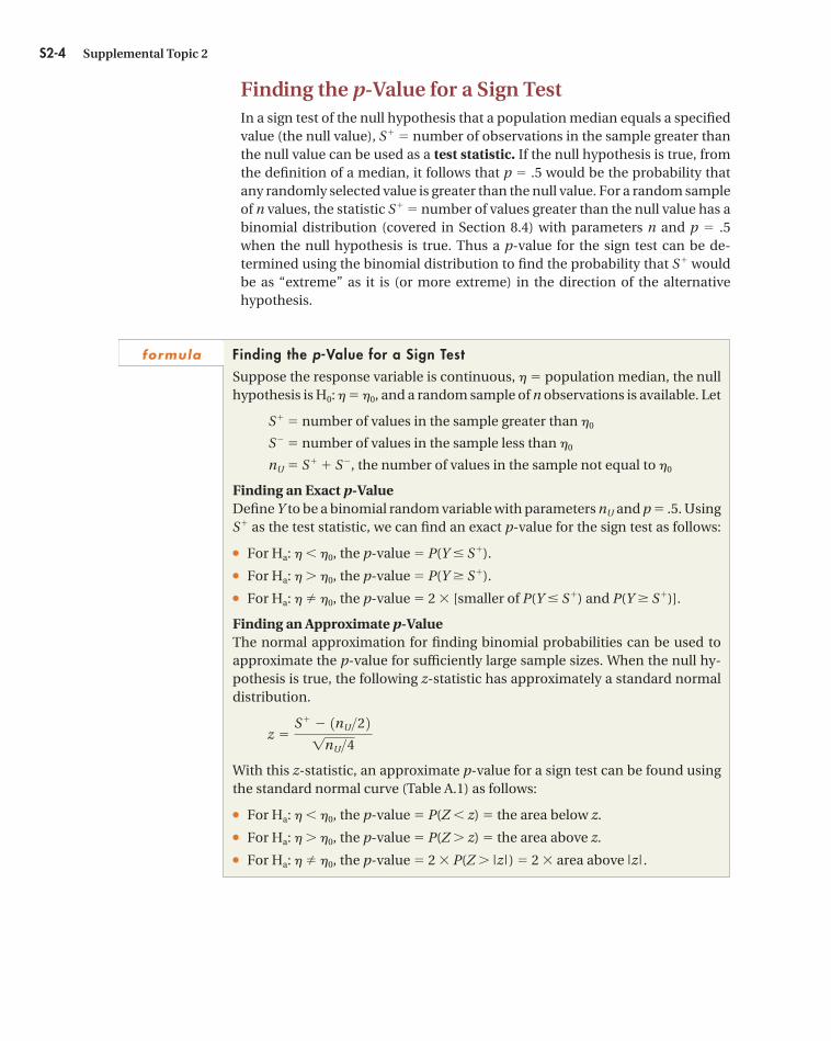
Finding an Approximate p-ValueThe normal approximation for finding binomial probabilities can be used toapproximate the p-value for sufficiently large sample sizes. When the null hy-pothesis is true, the following z-statistic has approximately a standard normaldistribution.

With this z-statistic, an approximate p-value for a sign test can be found usingthe standard normal curve (Table A.1) as follows:

� For Ha: h� h0, the p-value � P(Z � z) � the area below z.

� For Ha: h� h0, the p-value � P(Z � z) � the area above z.

� For Ha: h� h0, the p-value � 2 P(Z � |z|) � 2 area above |z| .

z �S� � 1nU>2 21nU>4

formula

S2-W3527 9/28/05 4:03 PM Page S2-4

Watch a video example at http://1pass.thomson.com or on your CD.

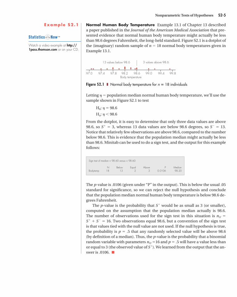
Example S2.1 Normal Human Body Temperature Example 13.1 of Chapter 13 describeda paper published in the Journal of the American Medical Association that pre-sented evidence that normal human body temperature might actually be lessthan 98.6 degrees Fahrenheit, the long-held standard. Figure S2.1 is a dotplot ofthe (imaginary) random sample of n � 18 normal body temperatures given inExample 13.1.

Letting h� population median normal human body temperature, we’ll use thesample shown in Figure S2.1 to test

H0: h� 98.6

Ha: h� 98.6

From the dotplot, it is easy to determine that only three data values are above98.6, so S� � 3, whereas 13 data values are below 98.6 degrees, so S� � 13. Notice that relatively few observations are above 98.6, compared to the numberbelow 98.6. This is evidence that the population median might actually be lessthan 98.6. Minitab can be used to do a sign test, and the output for this examplefollows:

The p-value is .0106 (given under “P” in the output). This is below the usual .05standard for significance, so we can reject the null hypothesis and concludethat the population median normal human body temperature is below 98.6 de-grees Fahrenheit.

The p-value is the probability that S� would be as small as 3 (or smaller),computed on the assumption that the population median actually is 98.6.The number of observations used for the sign test in this situation is nU �

S� � S� � 16. Two observations equal 98.6, but a convention of the sign testis that values tied with the null value are not used. If the null hypothesis is true,the probability is p � .5 that any randomly selected value will be above 98.6(by definition of a median). Thus, the p-value is the probability that a binomialrandom variable with parameters nU �16 and p � .5 will have a value less thanor equal to 3 (the observed value of S�). We learned from the output that the an-swer is .0106. �

Sign test of median = 98.60 versus < 98.60

N Below Equal Above P MedianBodytemp 18 13 2 3 0.0106 98.20


Body temperature97.0

13 values below 98.6 3 values above 98.6

97.4 97.8 98.2 98.6 99.0 99.4 99.8

Figure S2.1 ❚ Normal body temperature for n � 18 individuals

S2-W3527 9/28/05 4:03 PM Page S2-5

Example S2.2 Heights of Male Students and Their Fathers Do male college students tendto be taller than their fathers? The UCDavis2 dataset on the CD for this book in-cludes student height (inches) and father’s height (reported by the student) forn � 76 male students in an elementary statistics class. To compare the heightsof sons and fathers, we can compute difference � student height � father’s heightfor each of the 76 men in the sample. The sample of differences is graphed inFigure S2.2. One notable feature of the plot is the outlier. One student reportedthat he is 37 inches taller than his father! A positive difference (�0) occurswhen the student is taller than his father, and a negative difference occurs whenthe student is shorter. Notice in Figure S2.2 that more values fall above 0 thanbelow.

Figure S2.2 ❚ Difference between student height and father’s height for n � 76 college men

It is believed that humans are gradually getting taller from one generation tothe next, so let’s use the sign test to test the following:

H0: h� 0 (population median difference � 0)

Ha: h� 0 (population median difference is greater than 0)

Minitab output for this situation follows:

The p-value given in the output is .0032 (under “P”), so we can reject the nullhypothesis and conclude that the population median difference is greater than0. In particular, this indicates that students in the population represented bythe sample tend to be taller than their fathers. The sample median is given in

Sign test of median = 0.00000 versus > 0.00000

N N* Below Equal Above P MedianDifference 76 10 21 11 44 0.0032 1.000

Difference in heights (in.)–10 0 10 20 30 40


Using Minitab to Do a Sign TestFor paired data, it will be necessary to first calculate a column of differencesbetween the paired measurements.

� Use StatbNonparametricsb1-Sample Sign.

� In the box labeled “Variables,” specify the column that contains the data.

� Click the Test Median radio button and enter the null value in the adja-cent box.

� Select the desired alternative hypothesis.

MINITAB t ip

S2-W3527 9/28/05 4:03 PM Page S2-6

the output; the median difference in the sample was 1 inch. We also see in theoutput that S� � 44 (number of differences above 0) and S� � 21 (number ofdifferences below 0). The difference was equal to 0 for 11 students. The alterna-tive hypothesis is a “greater than” hypothesis, so the p-value was computedas the probability that S� would be greater than or equal to 44, assuming thatthe null hypothesis is true. The exact p-value can be found as P(Y 44) �

1 � P(Y � 43) � 1 � .997 � .003, where Y is a binomial random variable withparameters nU � 65 and p � .5. A z-statistic could be also be used to find the p-value. In this example,

Using this z-statistic, we find the approximate p-value to be P(Z � 2.85) �

.0022. �

z �S� � 1nU>2 21nU>4 �

44 � 165>2 2165>4 � 2.85


S2.1 Exercises are on page S2-19.

Hypotheses for Discrete VariablesWhen the response variable is discrete, the null hypothesis should be writ-ten as H0: P(X � h0) � P(X � h0) where X denotes the response variable. Forcontinuous variables, this is the same as writing that h0 is the populationmedian, but this is not the case for discrete variables, owing to the nonzeroprobability for P(X � h0). For discrete variables, the two possible one-sidedalternative hypotheses are

Ha: P(X � h0) � P(X � h0) (X below h0 is more probable than Xabove h0.)

or

Ha: P(X � h0) � P(X � h0) (X below h0 is less probable than Xabove h0.)

The two-sided alternative hypothesis can be written as

Ha: P(X � h0) � P(X � h0) (X below h0 and X above h0 are not equallyprobable.)

technical note

S2.2 The Two-Sample Rank-Sum TestThe Wilcoxon rank-sum test, also known as the Mann–Whitney test andsometimes called the Mann–Whitney–Wilcoxon test, is a nonparametric alter-native to the two-sample t-test for comparing two means described in Section13.4 of Chapter 13. Usually, we will refer to this test simply as the two-samplerank-sum test. It can be used to compare two populations when the variableof interest is either quantitative or ordinal and the data are from two indepen-dent samples. The hypotheses of interest concern whether or not values in onepopulation tend to be larger than values in the other population. Some ex-

S2-W3527 9/28/05 4:03 PM Page S2-7

amples of research questions that could be addressed using a two-sample rank-sum test follow:

1. Do the resting pulse rates of women tend to be greater than the restingpulse rates of men?

2. Do students who say that religion is very important in their life tend tomiss fewer classes than do students who say that religion is not veryimportant?

3. When people rate how much they like rap music on a scale of 1 (don’tlike) to 6 (like a lot), do individuals from big cities tend to give rap higherratings than individuals from small towns do?

The Null and Alternative Hypotheses for the Two-Sample Rank-Sum TestThe null and alternative hypotheses for the two sample rank-sum test can bestated as

H0: No difference in the distribution of values in the two populations.Ha: The values in one population tend to be larger than values in the other.

The alternative will be one-sided if we specify which particular populationmight tend to have larger values. For instance, a statement that women tend tohave higher pulse rates than men would be a one-sided alternative hypothesis.

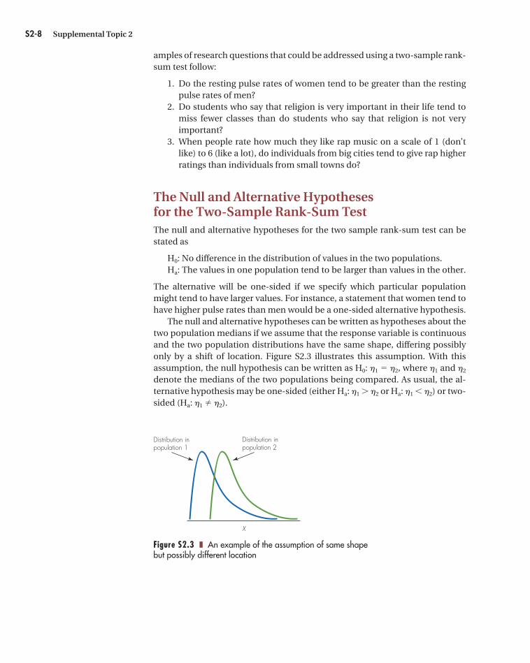
The null and alternative hypotheses can be written as hypotheses about thetwo population medians if we assume that the response variable is continuousand the two population distributions have the same shape, differing possiblyonly by a shift of location. Figure S2.3 illustrates this assumption. With thisassumption, the null hypothesis can be written as H0: h1 � h2, where h1 and h2

denote the medians of the two populations being compared. As usual, the al-ternative hypothesis may be one-sided (either Ha: h1 � h2 or Ha: h1 � h2) or two-sided (Ha: h1 � h2).


X

Distribution inpopulation 1

Distribution inpopulation 2

Figure S2.3 ❚ An example of the assumption of same shape but possibly different location

S2-W3527 9/28/05 4:03 PM Page S2-8


The Rank-Sum StatisticThe two-sample rank-sum test is based on ranks that are assigned to the ob-served values in the two samples. The rank of an observation is its location inthe ordered list of data, where the data are ordered from smallest to largest. Therank is 1 for the smallest data value, 2 for the second smallest value, and so on.For instance, the ranks for the values 65, 62, 67 are 2, 1, 3. When two or more ob-servations have the same value, the rank for each observation is the midrank,or average, of the lowest and highest ranks that would have been given if thevalues had not been tied. For example, the ranks for the ordered list of values60, 65, 65, 67, 70 are 1, 2.5, 2.5, 4, 5, respectively. The two observations equal to65 are tied for second and third place in the ordered list, so each is given therank 2.5, the average of 2 and 3.

The test statistic for the two-sample rank-sum test is W � sum of the ranks(within the overall dataset) for the observations in the first sample. The proce-dure for determining W is simple:

1. Combine the data from two samples and assign ranks to the values as 1 � smallest value, 2 � second smallest, and so on.

2. When observations have the same value, assign the midrank of the tiedvalues to each of the tied values.

3. Find W � sum of ranks for the values in sample 1.

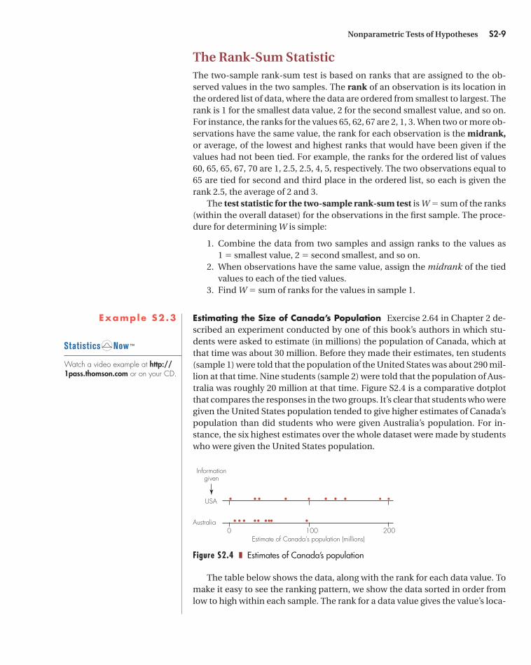
Example S2.3 Estimating the Size of Canada’s Population Exercise 2.64 in Chapter 2 de-scribed an experiment conducted by one of this book’s authors in which stu-dents were asked to estimate (in millions) the population of Canada, which atthat time was about 30 million. Before they made their estimates, ten students(sample 1) were told that the population of the United States was about 290 mil-lion at that time. Nine students (sample 2) were told that the population of Aus-tralia was roughly 20 million at that time. Figure S2.4 is a comparative dotplotthat compares the responses in the two groups. It’s clear that students who weregiven the United States population tended to give higher estimates of Canada’spopulation than did students who were given Australia’s population. For in-stance, the six highest estimates over the whole dataset were made by studentswho were given the United States population.

Figure S2.4 ❚ Estimates of Canada’s population

The table below shows the data, along with the rank for each data value. Tomake it easy to see the ranking pattern, we show the data sorted in order fromlow to high within each sample. The rank for a data value gives the value’s loca-

Estimate of Canada's population (millions)0

Australia

USA

Informationgiven

100 200


S2-W3527 9/28/05 4:03 PM Page S2-9

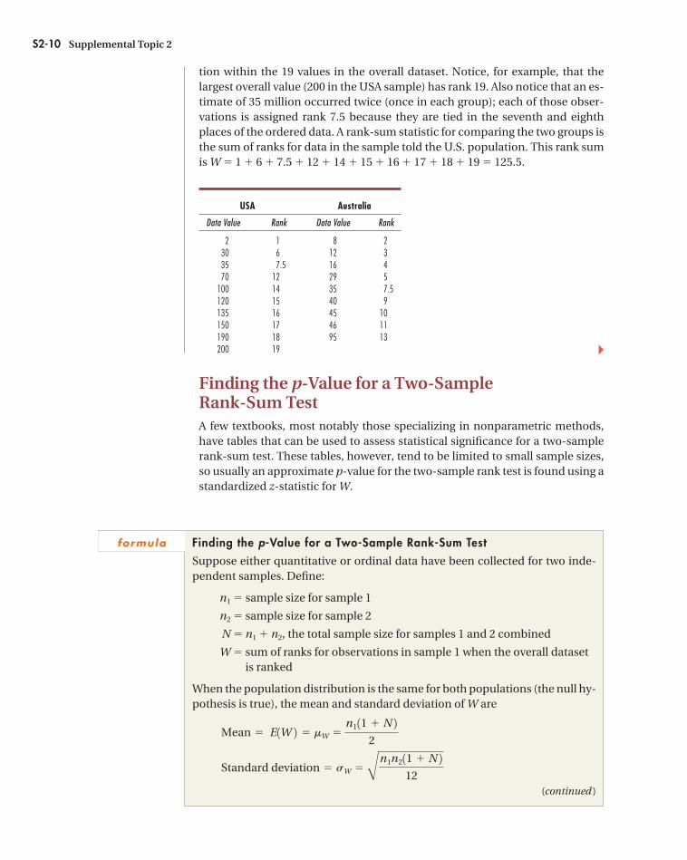
tion within the 19 values in the overall dataset. Notice, for example, that thelargest overall value (200 in the USA sample) has rank 19. Also notice that an es-timate of 35 million occurred twice (once in each group); each of those obser-vations is assigned rank 7.5 because they are tied in the seventh and eighthplaces of the ordered data. A rank-sum statistic for comparing the two groups isthe sum of ranks for data in the sample told the U.S. population. This rank sumis W � 1 � 6 � 7.5 � 12 � 14 � 15 � 16 � 17 � 18 � 19 � 125.5.

USA Australia

Data Value Rank Data Value Rank

2 1 8 230 6 12 335 7.5 16 470 12 29 5

100 14 35 7.5120 15 40 9135 16 45 10150 17 46 11190 18 95 13200 19 �

Finding the p-Value for a Two-Sample Rank-Sum TestA few textbooks, most notably those specializing in nonparametric methods,have tables that can be used to assess statistical significance for a two-samplerank-sum test. These tables, however, tend to be limited to small sample sizes,so usually an approximate p-value for the two-sample rank test is found using astandardized z-statistic for W.


Finding the p-Value for a Two-Sample Rank-Sum TestSuppose either quantitative or ordinal data have been collected for two inde-pendent samples. Define:

n1 � sample size for sample 1

n2 � sample size for sample 2

N � n1 � n2, the total sample size for samples 1 and 2 combined

W � sum of ranks for observations in sample 1 when the overall datasetis ranked

When the population distribution is the same for both populations (the null hy-pothesis is true), the mean and standard deviation of W are

(continued )

Standard deviation � sW � Bn1n211 � N 212

Mean � E1W 2 � mW �n111 � N 2

2

formula

S2-W3527 9/28/05 4:03 PM Page S2-10

Example S2.3 (cont.) p-Value for Testing Whether Information Given Affects Estimates of Can-ada’s Population The experiment was done to determine whether the infor-mation given would influence the estimate of Canada’s population. Specifically,it was believed that people who were told the U.S. population would tend to givehigher estimates than people who were told the Australia population.

The null and alternative hypotheses about the populations represented bythe two samples can be stated as

H0: No difference in the population distribution of values guessed for thetwo conditions.

Ha: Estimates made by people told the U.S. population tend to be larger thanestimates made by people told the Australia population.

To find the p-value, we can use the normal curve approximation describedabove. We found that the sum of ranks for the U.S. sample is W � 125.5, andthe sample sizes are n1 � 10 (U.S. sample), n2 � 9 (Australia sample), and N �

10 � 9 � 19 overall. Details for finding the z-statistic are

Because the alternative is a “greater than” hypothesis, the p-value is P(Z � 2.08),the area to the right of z � 2.08 under a standard normal curve. UtilizingTable A.1, we find that P(Z � 2.08) � 1 � P(Z � 2.08) � 1 � .9812 � .0188 � .02.The p-value is below the usual .05 standard used for significance, so we canconclude that the experiment is evidence that estimates of Canada’s populationby people who were told the U.S. population size will tend to be higher than es-timates by people who were told the Australia population size. �

z � 1125.5 � 100 2 >12.25 � 2.08

Standard deviation � sW � B 110 2 19 2 11 � 9 212

� 12.25

E1W 2 � mW � 31011 � 19 2 >2 4 � 100


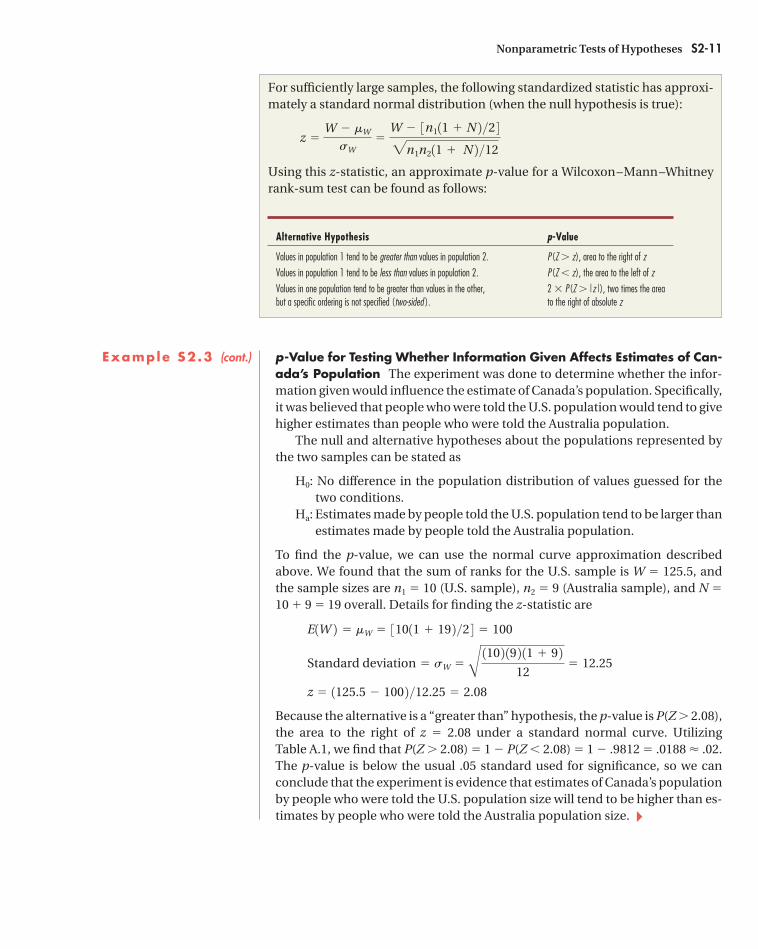
For sufficiently large samples, the following standardized statistic has approxi-mately a standard normal distribution (when the null hypothesis is true):

Using this z-statistic, an approximate p-value for a Wilcoxon–Mann–Whitneyrank-sum test can be found as follows:

Alternative Hypothesis p-Value

Values in population 1 tend to be greater than values in population 2. P(Z � z), area to the right of z

Values in population 1 tend to be less than values in population 2. P(Z � z), the area to the left of z

Values in one population tend to be greater than values in the other, 2 P(Z � |z |), two times the area but a specific ordering is not specified (two-sided ). to the right of absolute z

z �W � mW

sW�

W � 3n111 � N 2 >2 42n1n211 � N 2 >12

S2-W3527 9/28/05 4:03 PM Page S2-11

Example S2.3 (cont.) Minitab Output for the Population of Canada Experiment In Minitab,the two-sample rank-sum test is called the Mann–Whitney test. The Mann–Whitney test for our estimates of Canada’s population follows:

The last line gives a p-value that is adjusted for the presence of tied observationsin the data, and the next-to-last line gives a p-value that is not adjusted for ties.Here, the two p-values are identical; they rarely will differ by very much. Thephrase is significant at used in the last two lines can be interpreted as “the p-value is.” Notice that the output contains references to the population me-dians “ETA1” and “ETA2.” The next-to-last line includes information about thenull hypothesis (ETA1 � ETA2) and alternative hypothesis (ETA1 � ETA2) forthe test. �

S2.3 The Wilcoxon Signed-Rank TestThe Wilcoxon signed-rank test (not to be confused with the Wilcoxon rank-sum test in the previous section) is used to test hypotheses about the median ofone population. As with the sign test and the one-sample t-test, the signed-ranktest can be used either to examine a single response variable or to examine thedifference between paired measurements. Most often, in practice, the test is ap-plied to paired data. An important necessary condition for using this test is thatthe response variable have a symmetric (but not necessarily bell-shaped) dis-tribution in the population; the signed-rank test should not be used when thedata are skewed.

The specific hypotheses tested are the same as those for the sign test whenthe response is continuous. Again, we will use the symbol h (“eta”) to representthe population median. Thus, the null hypothesis for a signed-rank test couldbe written as

H0: h� h0 (population median equals a specified value)

USA N = 10 Median = 110.00Australi N = 9 Median = 35.00Point estimate for ETA1-ETA2 is 72.5095.5 Percent CI for ETA1-ETA2 is (1.02,123.01)W = 125.5Test of ETA1 = ETA2 vs ETA1 > ETA2 is significant at 0.0206The test is significant at 0.0206 (adjusted for ties)



Using Minitab to Do a Two-Sample Rank-Sum TestThe data for the two samples must be in two separate columns.

� Use StatbNonparametricsbMann–Whitney.

� Specify the columns containing the data for samples 1 and 2 in the boxeslabeled “Sample 1” and “Sample 2.”


MINITAB t ip

S2-W3527 9/28/05 4:03 PM Page S2-12

The alternative hypothesis can be one-sided (either Ha: h � h0 or Ha: h � h0) or two-sided (Ha: h � h0). When the alternative hypothesis is one-sided, the null hypothesis can be written to include an inequality in the opposite direc-tion. For paired differences, the null value of interest in most situations is h0 �0(“no difference”).

The Test Statistic for the Wilcoxon Signed-Rank TestThe procedure for determining the test statistic used in the Wilcoxon signed-rank test is as follows:

1. For each data value xi, record whether the value is below h0 (a negativedifference) or above h0 (a positive difference). Values equal to h0 are notused in the test.

2. For each data value xi, calculate |xi � h0|, the absolute difference betweenthe data value and the null value.

3. Assign ranks to the absolute differences computed in the previous step.(Do not include observations for which the difference � 0.)

4. The test statistic is T � � sum of ranks for data values above h0 (the posi-tive differences).

Notice that T � will be influenced both by how many observations are above thenull value (as in the sign test) and by how far the positive differences are fromthe null value (not a feature of the sign test).

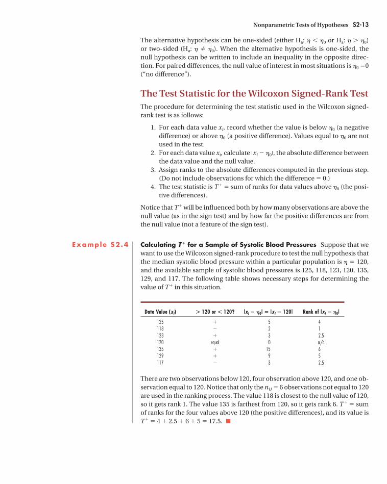
Example S2.4 Calculating T � for a Sample of Systolic Blood Pressures Suppose that wewant to use the Wilcoxon signed-rank procedure to test the null hypothesis thatthe median systolic blood pressure within a particular population is h � 120,and the available sample of systolic blood pressures is 125, 118, 123, 120, 135,129, and 117. The following table shows necessary steps for determining thevalue of T � in this situation.

Data Value (xi) b 120 or a 120? |xi � h0| � |xi � 120| Rank of |xi � h0|

125 � 5 4.0118 � 2 1.0123 � 3 2.5120 equal 0 n/a135 � 15 6.0129 � 9 5.0117 � 3 2.5

There are two observations below 120, four observation above 120, and one ob-servation equal to 120. Notice that only the nU � 6 observations not equal to 120are used in the ranking process. The value 118 is closest to the null value of 120,so it gets rank 1. The value 135 is farthest from 120, so it gets rank 6. T � � sumof ranks for the four values above 120 (the positive differences), and its value isT � � 4 � 2.5 � 6 � 5 � 17.5. �


S2-W3527 9/28/05 4:03 PM Page S2-13


Example S2.5 Difference Between Student Height and Mother’s Height for CollegeWomen The UCDavis2 dataset on the CD for this book includes studentheight (inches) and mother’s height for n � 132 women in an elementary statis-tics class. For each woman, we can compute difference � own height � mother’sheight, and a histogram of those differences is shown in Figure S2.5. Notice thatthe majority of observations are above 0, so more students are taller than theirmothers rather than being shorter. Also notice that the shape of the histogramis more or less symmetric, so the Wilcoxon signed-rank test could be used to testhypotheses about the population median difference between student heightand mother’s height.

Finding the p-Value for a Wilcoxon Signed-Rank TestIn general, a relatively large value of T � may be evidence that h� h0, and a rela-tively small value may be evidence that h � h0. An approximate p-value forevaluating the statistical significance of T � can be found by using a standard-ized z-statistic that has approximately a standard normal distribution.


Finding the p-Value for a Wilcoxon Signed-Rank TestSuppose the response variable is continuous and symmetric, h � populationmedian, the null hypothesis is H0: h � h0, and a random sample of n observa-tions x1, x2, . . . , xn is available. Let

T � � Wilcoxon signed-rank statistic

nU � The number of values in the sample not equal to h0, the samplesize used for the test

When the null hypothesis is true (h � h0), the mean and standard deviation ofT � are

Standard deviation

For sufficiently large samples, the following standardized statistic has approxi-mately a standard normal distribution (when the null hypothesis is true):

With this z-statistic, an approximate p-value for a Wilcoxon signed-rank testcan be found using the standard normal curve (Table A.1) as follows:

� For Ha: h� h0, the p-value � P(Z � z) � the area below z.

� For Ha: h� h0, the p-value � P(Z � z) � the area above z.

� For Ha: h� h0, the p-value � 2 P(Z � |z|) � 2 area above |z|.

z �T � � mT�

sT�

�T � � 3nU 1nU � 1 2 >4 42nU 1nU � 1 2 12nU � 1 2 >24

� sT� � BnU 1nU � 1 2 12nU � 1 224

Mean � E1T � 2 � mT� �nU 1nU � 1 2

4

formula

S2-W3527 9/28/05 4:03 PM Page S2-14

We’ll use the Wilcoxon signed-rank procedure to test

H0: h� 0 (population median difference � 0)

Ha: h� 0 (population median difference is greater than 0)

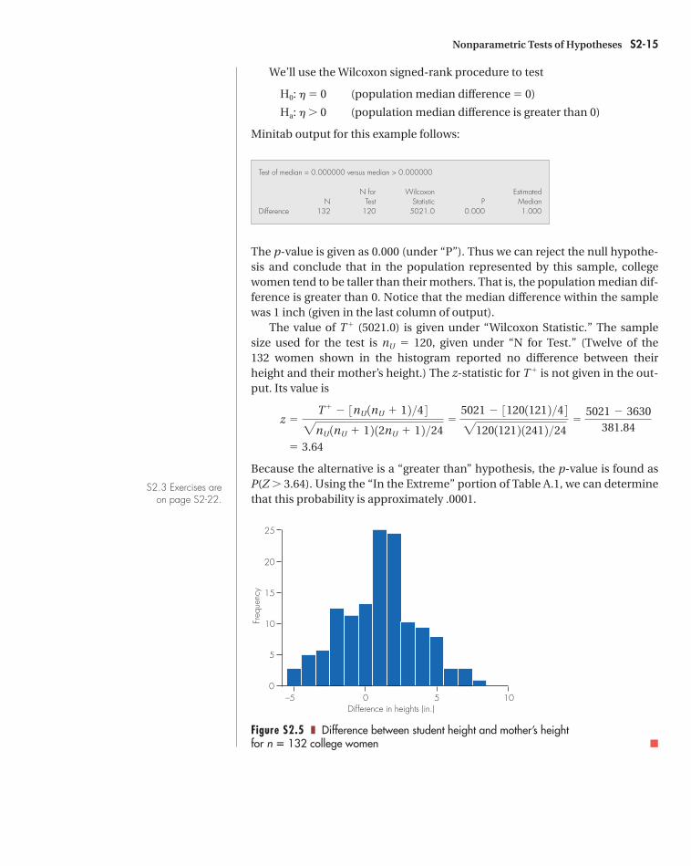
Minitab output for this example follows:

The p-value is given as 0.000 (under “P”). Thus we can reject the null hypothe-sis and conclude that in the population represented by this sample, collegewomen tend to be taller than their mothers. That is, the population median dif-ference is greater than 0. Notice that the median difference within the samplewas 1 inch (given in the last column of output).

The value of T � (5021.0) is given under “Wilcoxon Statistic.” The samplesize used for the test is nU � 120, given under “N for Test.” (Twelve of the132 women shown in the histogram reported no difference between theirheight and their mother’s height.) The z-statistic for T � is not given in the out-put. Its value is

Because the alternative is a “greater than” hypothesis, the p-value is found asP(Z � 3.64). Using the “In the Extreme” portion of Table A.1, we can determinethat this probability is approximately .0001.

� 3.64

z �T � � 3nU 1nU � 1 2 >4 42nU 1nU � 1 2 12nU � 1 2 >24

�5021 � 31201121 2 >4 421201121 2 1241 2 >24

�5021 � 3630

381.84

Test of median = 0.000000 versus median > 0.000000

N for Wilcoxon EstimatedN Test Statistic P Median

Difference 132 120 5021.0 0.000 1.000


25

20

15

10

5

0

Difference in heights (in.)

Freq

uenc

y

0 105–5

Figure S2.5 ❚ Difference between student height and mother’s heightfor n � 132 college women �


S2-W3527 9/28/05 4:03 PM Page S2-15

S2.4 The Kruskal–Wallis TestWe briefly discussed the Kruskal–Wallis test in Section 16.3 of Chapter 16.Here, we provide more details of the test. The Kruskal–Wallis test is used tocompare three or more populations when the response variable is quantitativeand the data are from independent random samples from the populations be-ing compared. Some examples of questions that could be examined using aKruskal–Wallis test follow:

1. Are testosterone levels the same for men in four different occupations(teachers, doctors, firefighters, and lawyers)?

2. Is the number of classes missed per week the same for students who saythat religion is very important, students who say that religion is fairly im-portant, and students who say that religion is not very important?

3. Students rate how much they like Rap music on a scale of 1 (don’t like)to 6 (like a lot). Do the ratings differ by type of hometown (big city, sub-urban, small town, rural)?

The precise nature of hypotheses for the Kruskal–Wallis test depends onwhat assumptions, if any, are made about the distribution of the response vari-able in the populations. In all circumstances, the null hypothesis and alterna-tive hypothesis could be written as

H0: The distribution of values is the same for all populations.Ha: Values in at least one population tend to be larger (or smaller) than val-

ues in the other populations.

If we can assume that the variable of interest is continuous and that the popu-lation distributions all have the same shape (see Figure S2.3 in Section S2.2 foran example), we can express the hypotheses as statements about populationmedians. In this case, the null and alternative hypotheses are

H0: h1 � h2 � . . . � hk (population medians are equal)Ha: At least one population median differs from the others.

We wrote the hypotheses in this manner in Section 16.3, although we did notstate the assumption that the population distributions all have the same shape.


Using Minitab to Do a Wilcoxon Signed-Rank TestFor paired data it will be necessary to first calculate a column of differencesbetween the paired measurements.

� Use StatbNonparametricsb1-Sample Wilcoxon.

� In the box labeled “Variables,” specify the column that contains the data.

� Click the Test Median radio button and enter the null value in the adja-cent box.


MINITAB t ip

S2-W3527 9/28/05 4:03 PM Page S2-16


Determining the Test Statistic for the Kruskal–Wallis TestThe value of the test statistic for the Kruskal–Wallis test is found by using thesesteps:

1. Assign ranks to all values within the overall dataset (all samples com-bined). The ranking procedure is the same as it was for the two-samplerank-sum test. The smallest data value is assigned rank 1, the secondsmallest is assigned rank 2, and so on. Use midranks for tied observations.

2. For each independent sample, find the average rank assigned to obser-vations within that sample. Let represent the average rank in sample i.

3. Let ni � sample size in sample i, N � the total of the sample sizes for allgroups, and k � number of independent samples. The Kruskal–Wallisstatistic is

The average rank for all observations in the combined dataset is (1 � N )>2.Notice that the test statistic is a function of the difference between the av-erage rank in each sample and the overall average rank for the dataset, (1 � N )>2.

Finding the p-Value for a Kruskal–Wallis TestWhen the null hypothesis is true, the test statistic, H, has a chi-square distribu-tion with degrees of freedom � number of samples � 1 � k � 1. The p-value fora Kruskal–Wallis test is found as the probability that a chi-square variable withk � 1 degrees of freedom will have a value greater than the value of H. Table A.5in the Appendix can be used to approximate the p-value.

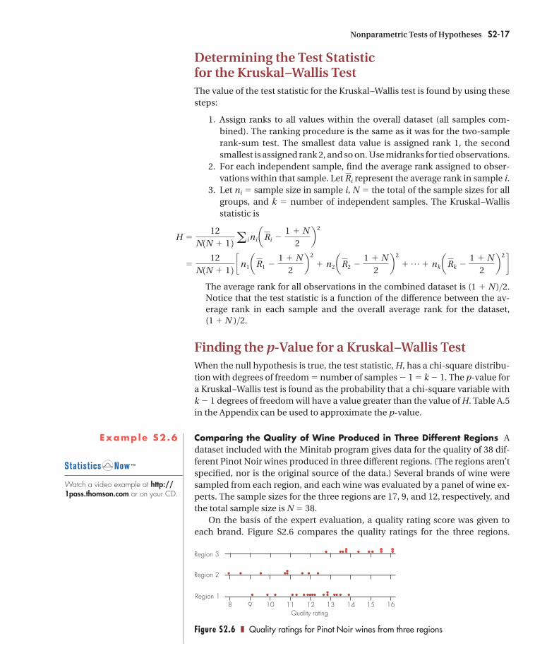
Example S2.6 Comparing the Quality of Wine Produced in Three Different Regions Adataset included with the Minitab program gives data for the quality of 38 dif-ferent Pinot Noir wines produced in three different regions. (The regions aren’tspecified, nor is the original source of the data.) Several brands of wine weresampled from each region, and each wine was evaluated by a panel of wine ex-perts. The sample sizes for the three regions are 17, 9, and 12, respectively, andthe total sample size is N � 38.

On the basis of the expert evaluation, a quality rating score was given to each brand. Figure S2.6 compares the quality ratings for the three regions.

Figure S2.6 ❚ Quality ratings for Pinot Noir wines from three regions

Quality rating8

Region 1

Region 2

Region 3

10 11 12 13 14 159 16

�12

N1N � 1 2 cn1 aR1 �1 � N

2b 2

� n2 aR2 �1 � N

2b 2

� p � nk aRk �1 � N

2b 2 d

H �12

N1N � 1 2 a i ni aRi �1 � N

2b 2

Ri


S2-W3527 9/28/05 4:03 PM Page S2-17

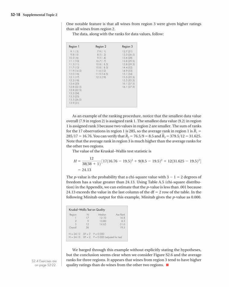
One notable feature is that all wines from region 3 were given higher ratingsthan all wines from region 2.

The data, along with the ranks for data values, follow:

As an example of the ranking procedure, notice that the smallest data valueoverall (7.9 in region 2) is assigned rank 1. The smallest data value (9.2) in region1 is assigned rank 3 because two values in region 2 are smaller. The sum of ranksfor the 17 observations in region 1 is 285, so the average rank in region 1 is �

285>17 � 16.76. You can verify that � 76.5>9 � 8.5 and � 379.5>12 � 31.625.Note that the average rank in region 3 is much higher than the average ranks forthe other two regions.

The value of the Kruskal–Wallis test statistic is

The p-value is the probability that a chi-square value with 3 � 1 � 2 degrees offreedom has a value greater than 24.13. Using Table A.5 (chi-square distribu-tion) in the Appendix, we can estimate that the p-value is less than .001 because24.13 exceeds the value in the last column of the df � 2 row of the table. In thefollowing Minitab output for this example, Minitab gives the p-value as 0.000.

We barged through this example without explicitly stating the hypotheses,but the conclusion seems clear when we consider Figure S2.6 and the averageranks for three regions. It appears that wines from region 3 tend to have higherquality ratings than do wines from the other two regions. �

Kruskal–Wallis Test on Quality

Region N Median Ave Rank1 17 12.10 16.82 9 10.80 8.53 12 14.65 31.6

Overall 38 19.5

H = 24.13 DF = 2 P = 0.000H = 24.15 DF = 2 P = 0.000 (adjusted for ties)

� 24.13

H �12

38138 � 1 2 317116.76 � 19.5 22 � 918.5 � 19.5 22 � 12131.625 � 19.5 22 4

R3R2

R1

Region 1 Region 2 Region 3

9.1 ( 3) 7.9 ( 1) 12.7 (21)9.8 ( 5) 8.5 ( 2) 13.5 (26.5)

10.3 ( 6) 9.5 ( 4) 13.6 (28)11.1 (10) 10.7 ( 7) 13.8 (29.5)11.3 (11) 10.8 ( 8.5) 13.8 (29.5)11.7 (13) 10.8 ( 8.5) 14.4 (32)11.9 (14.5) 11.6 (12) 14.9 (33)12.0 (16) 11.9 (14.5) 15.1 (34)12.1 (17) 12.3 (19) 15.5 (35.5)12.2 (18) 15.5 (35.5)12.6 (20) 16.1 (37.5)12.8 (22.5) 16.1 (37.5)12.8 (22.5)13.2 (24)13.3 (25)13.5 (26.5)13.9 (31)


S2.4 Exercises areon page S2-22.

S2-W3527 9/28/05 4:03 PM Page S2-18

� Denotes basic skills exercises� Denotes dataset is available in StatisticsNow at http://

1pass.thomson.com or on your CD but is not required to solve the exercise.

Bold-numbered exercises have answers in the back of the text andfully worked solutions in the Student Solutions Manual.

Go to the StatisticsNow website at http://1pass.thomson.com to:• Assess your understanding of this chapter• Check your readiness for an exam by taking the Pre-Test quiz and

exploring the resources in the Personalized Learning Plan

Section S2.1S2.1 In each situation, explain whether it would be appro-

priate to use a sign test to analyze the question of in-terest. If so, write the null and alternative hypothesesin words, and again using proper statistical notation.a. Resting pulse rates are measured for n � 25 adult

women. Is the median pulse rate of women equal to72 or is it greater than 72?

b. Are the median heights of 11-year-old girls and 11-year-old boys the same, or are they different?

c. Blood pressures are measured in the morning andagain at night for each individual in a random

sample of n � 100 college students. On average, arethe morning and nighttime blood pressure mea-surements about equal, or does blood pressure tendto be higher at night?

S2.2 � A sample of n � 63 college men reports their actualand ideal (desired) weights (pounds). The difference,computed as actual � ideal, was positive for 28 of themen, was negative for 19 others, and was equal to 0 forthe remaining 16 men. (Data source: idealwtmen onthe CD for this book.)a. Suppose the data are used to test the null hypothe-

sis that the population median difference is 0 versusthe alternative hypothesis that the population me-dian difference is greater than 0. What are the valuesof S�, S�, and nU?

b. Explain how a p-value would be found in this situa-tion. Specifically, what probability should be found,and what are the parameters of the binomial distri-bution that would be used to determine it?

c. Compute the value of the z-statistic that could beused to find an approximate p-value for this prob-lem.

d. Find the p-value based on the z-statistic, and write aconclusion about the hypotheses.

S2.3 Twenty individuals each place as many beans as theycan into a container during a 30-second time period


� Basic skills � Dataset available but not required Bold-numbered exercises answered in the back

Key Terms

Introductionnonparametric test, S2-2robust, S2-2resistant, S2-2

Section S2.1sign test, S2-3test statistic for sign test, S2-4p-value for sign test, S2-4

Section S2.2Wilcoxon rank-sum test, S2-7Mann–Whitney test, S2-7two-sample rank-sum test, S2-7rank, S2-9midrank, S2-9test statistic for two-sample rank-sum test,

S2-9p-value for two-sample rank-sum test,

S2-10, S2-11

Section S2.3Wilcoxon signed-rank test, S2-12test statistic for signed-rank test, S2-13p-value for Wilcoxon signed-rank test,

S2-14

Section S2.4Kruskal–Wallis test, S2-16test statistic for Kruskal–Wallis test, S2-17p-value for Kruskal–Wallis test, S2-17

Exercises

Kruskal –Wallis Test� Use StatbNonparametricsbKruskal–Wallis.

� Specify the column containing the response data in the box labeled“Response.”

� Specify the column containing the group designations in the box labeled“Explanatory.”

MINITAB t ip

S2-W3527 9/28/05 4:03 PM Page S2-19

using their dominant hand and again using their non-dominant hand. The order of using the dominant andnondominant hands is randomly determined for eachperson. Thirteen individuals in the sample placedmore beans with their dominant hand, three peopleplaced more beans with their nondominant hand, andfour people placed the same number with each hand.Consider a sign test to determine whether the dataare statistically significant evidence that, in general,people are able to place more beans with their domi-nant hand.a. Write null and alternative hypotheses in words and

using statistical notation.b. What are the values of S�, S�, and nU?c. Refer to part (a). Carry out a sign test and state a

conclusion.S2.4 Suppose that a sample of 16 students at a university

is asked about how much they spent on textbooks forthe present semester, and the responses (in dollars)are as follows:

250, 450, 300, 279, 360, 300, 670, 50, 430, 350, 220,420, 375, 275, 360, 365

Consider a test of the null hypothesis that the popula-tion median amount spent is $400 (or more) versus thealternative hypothesis that the population median isless than $400.a. Write the null and alternative hypotheses using sta-

tistical notation.b. What is the value of the sample median amount

spent?c. What are the values of S �, S �, and nU?d. Explain how a p-value would be found in this situa-

tion. Specifically, what probability should be found,and what are the parameters of the binomial distri-bution that would be used to determine it?

e. Carry out a sign test and write a conclusion. Eitherfind an exact p-value using the binomial distribu-tion or use a z-statistic to find an approximate p-value.

S2.5 In a survey about music interests done in a statisticsclass at Penn State, students were asked to rate howmuch they like various types of music on a scale of 1(don’t like) to 6 (like a lot). The Minitab output givenfor this exercise is for a sign test for the differencebetween student ratings of punk and country music(computed as punk � country). The output indicatesthat the test is of whether the median difference is 0 ornot 0. Because the response is discrete with few pos-sible values, it is more appropriate to write H0 as P(dif-ference below 0) � P(difference above 0) and Ha asP(difference below 0) � P(difference above 0).

a. How many students said that they like punk musicmore than country music? How many said that they

Sign test of median � 0.00000 versus not � 0.00000

N Below Equal Above P Medianpunk � country 738 229 136 373 0.0000 1.000

like country better than punk? How many gave thetwo types of music the same rating?

b. What value is given in the output for the p-valueof the test? On the basis of this p-value, what is theappropriate conclusion? Write a conclusion in thecontext of this situation.

c. Find the value of the z-statistic that could be used tofind the p-value given in the output.

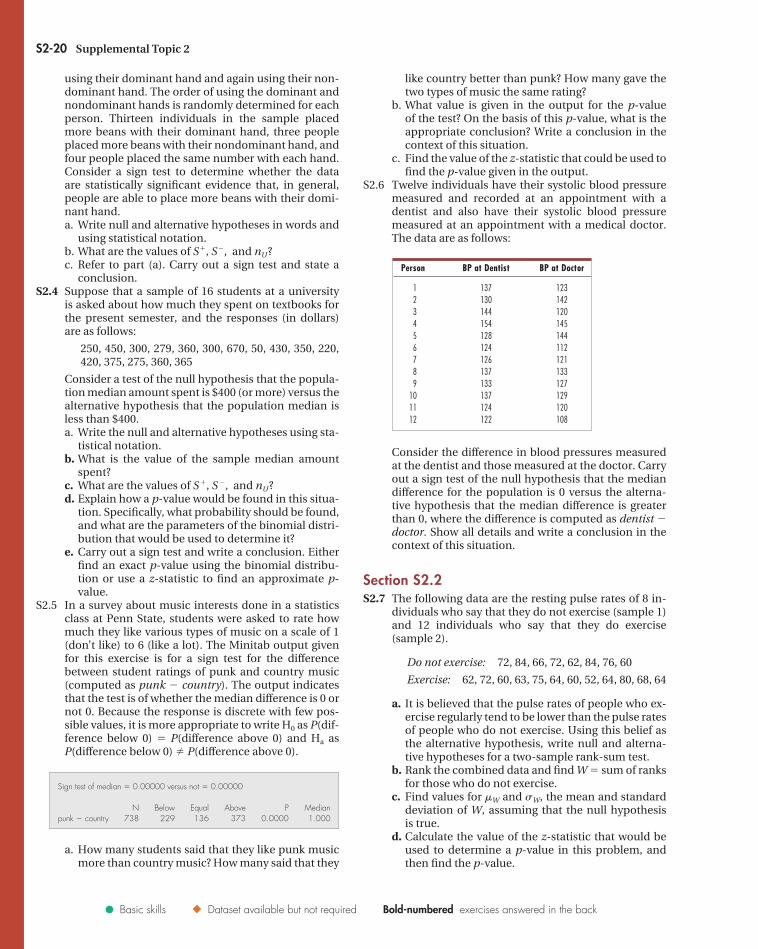
S2.6 Twelve individuals have their systolic blood pressuremeasured and recorded at an appointment with adentist and also have their systolic blood pressuremeasured at an appointment with a medical doctor.The data are as follows:

Consider the difference in blood pressures measuredat the dentist and those measured at the doctor. Carryout a sign test of the null hypothesis that the mediandifference for the population is 0 versus the alterna-tive hypothesis that the median difference is greaterthan 0, where the difference is computed as dentist �doctor. Show all details and write a conclusion in thecontext of this situation.

Section S2.2S2.7 The following data are the resting pulse rates of 8 in-

dividuals who say that they do not exercise (sample 1)and 12 individuals who say that they do exercise(sample 2).

Do not exercise: 72, 84, 66, 72, 62, 84, 76, 60

Exercise: 62, 72, 60, 63, 75, 64, 60, 52, 64, 80, 68, 64

a. It is believed that the pulse rates of people who ex-ercise regularly tend to be lower than the pulse ratesof people who do not exercise. Using this belief asthe alternative hypothesis, write null and alterna-tive hypotheses for a two-sample rank-sum test.

b. Rank the combined data and find W � sum of ranksfor those who do not exercise.

c. Find values for mW and sW, the mean and standarddeviation of W, assuming that the null hypothesisis true.

d. Calculate the value of the z-statistic that would beused to determine a p-value in this problem, andthen find the p-value.



Person BP at Dentist BP at Doctor

1 137 1232 130 1423 144 1204 154 1455 128 1446 124 1127 126 1218 137 1339 133 127

10 137 12911 124 12012 122 108

S2-W3527 9/28/05 4:03 PM Page S2-20

e. State a conclusion about the null and alternativehypotheses in the context of this situation.

S2.8 Suppose that 14 overweight individuals are dividedrandomly into two groups, with 7 in each group. Thefirst group is assigned to use a diet intended tocause weight loss, and the second group is assignedto use an exercise plan to lose weight. After threemonths, weight losses (pounds) in the two groups areas follows:

Diet plan: 10, 8, 12, 16, 0, 7, 35

Exercise plan: 12, 7, 2, 3, 5, 4, 9

a. Find the value of W, the test statistic for a two-sample rank-sum test that would compare the twomethods for losing weight. Give the details of howyou found W.

b. Carry out a two-sample rank-sum test (Mann–Whitney–Wilcoxon test) in which the alternativehypothesis is that median weight loss is greater ifdieting is the weight-loss method used. Show alldetails and state a conclusion in the context of thissituation.

S2.9 Refer to data given in Exercise S2.8. Explain why itwould not be advisable to use those data to do a two-sample t-test to compare the mean weight losses forthe two methods.

S2.10 Case Study 1.1 in Chapter 1 gave data for responsesby 189 Penn State students to the question “What’sthe fastest you have ever driven a car? mph.”The data showed that male respondents tended to re-port faster speeds than females. The following dataare responses to the same question for 14 men and 10women in a different statistics class at Penn State:

Males: 100, 95, 85, 130, 125, 90, 110, 120, 95, 92,120, 85, 105, 75

Females: 95, 110, 87, 55, 95, 105, 80, 90, 80, 70

Carry out a two-sample rank-sum test in which thealternative hypothesis is that the fastest speeds everdriven reported by men tend to be faster than thefastest speeds ever driven reported by women. Statethe hypotheses, show all details of the test, and statea conclusion in the context of this situation.

S2.11 Example S2.3 described an experiment in which in-dividuals were asked to estimate the population ofCanada. Some participants were given informationabout the population of the United States (condi-tion 1), and others were given information about thepopulation of Australia (condition 2). The same ex-periment was performed with a different group ofparticipants. Those data were given in Exercise 13.69and are given again here:

Condition 1 (n1 � 11): 20, 90, 1.5, 100, 132, 150,130, 130, 40, 200, 20

Condition 2 (n2 � 10): 12, 20, 10, 81, 15, 20, 30,20, 9, 10, 20

a. Find the sample medians for condition 1 (given U.S. population) and condition 2 (given Australia population).

b. Rank the combined set of 21 values, and find W � sum of ranks for condition 1.

c. Using the data given for this exercise, carry outa two-sample rank-sum test (Mann–Whitney–Wilcoxon test) of the same hypotheses tested inExample S2.3. State the hypotheses, show detailsof finding the p-value, and state a conclusion inthe context of this situation.

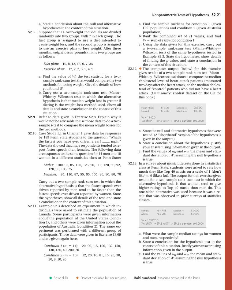
S2.12 � The computer output (below) for this exercisegives results of a two-sample rank-sum test (Mann–Whitney–Wilcoxon test) done to compare the mediancholesterol level of heart attack patients (measuredtwo days after the heart attack) to the median choles-terol of “control” patients who did not have a heartattack. (Data source: cholest dataset on the CD forthis book.)

a. State the null and alternative hypotheses that weretested. (A “shorthand” version of the hypotheses isgiven in the output.)

b. State a conclusion about the hypotheses. Justifyyour answer using information given in the output.

c. Find the values of mW and sW, the mean and stan-dard deviation of W, assuming the null hypothesisis true.

S2.13 In a survey about music interests done in a statisticsclass at Penn State, students were asked to rate howmuch they like Top 40 music on a scale of 1 (don’tlike) to 6 (like a lot). The output for this exercise givesresults for a two-sample rank-sum test in which thealternative hypothesis is that women tend to givehigher ratings to Top 40 music than men do. Thisone-sided alternative was used because it was a re-sult that was observed in prior surveys of statisticsclasses.

a. What were the sample median ratings for womenand men, respectively?

b. State a conclusion for the hypothesis test in thecontext of this situation. Justify your answer usinginformation given in the output.

c. Find the values of mW and sW, the mean and stan-dard deviation of W, assuming the null hypothesisis true.

Females N = 448 Median = 5.0000Males N = 283 Median = 4.0000

W = 183726.5Test of ETA1 = ETA2 vs ETA1 > ETA2 is significant at 0.0000

Heart Attack N = 28 Median = 268.00Control N = 30 Median = 187.00

W = 1140.0Test of ETA1 = ETA2 vs ETA1 > ETA2 is significant at 0.0000



S2-W3527 9/28/05 4:03 PM Page S2-21

d. Calculate the value of a z-statistic that could beused to determine a p-value in this problem.

Section S2.3S2.14 Refer to Exercise S2.4, in which data are given for

the amount spent on textbooks. Suppose a Wilcoxonsigned-rank procedure will be used to test the nullhypothesis that the population median amount spentis $400 (or more) versus the alternative hypothesisthat the population median is less than $400.a. Find the value of T �, the Wilcoxon signed-rank test

statistic. Show details.b. Calculate the value of the z-statistic that would be

used to determine a p-value in this problem, andthen find the p-value.

c. On the basis of the p-value found in part (b), whatconclusion can be made about the hypotheses?

S2.15 Refer to Exercise S2.6, in which data are given forblood pressures measured at a visit to a dentist anda visit to a doctor. Carry out a Wilcoxon signed-ranktest of the null hypothesis that the population me-dian difference is 0 versus the alternative hypothesisthat the median difference is greater than 0, wherethe difference is computed as dentist � doctor. Showall details, and write a conclusion in the context ofthis situation.

S2.16 Refer to Example S2.1 about normal human bodytemperature. The data are as follows:

98.2 97.8 99.0 98.6 98.2 97.8 98.4 99.798.2 97.4 97.6 98.4 98.0 99.2 98.6 97.197.2 98.5

Minitab output for a Wilcoxon signed-rank test of H0: h� 98.6 versus Ha: h� 98.6 is as follows:

a. Show the details for finding the value of T � (givenin the output as 27.0).

b. On the basis of the p-value given in the output,what conclusion can be reached about the hy-potheses? Write a conclusion in the context of thissituation.

S2.17 Refer to Exercise S2.16. Find values for and the mean and standard deviation of T �, assuming thenull hypothesis is true.

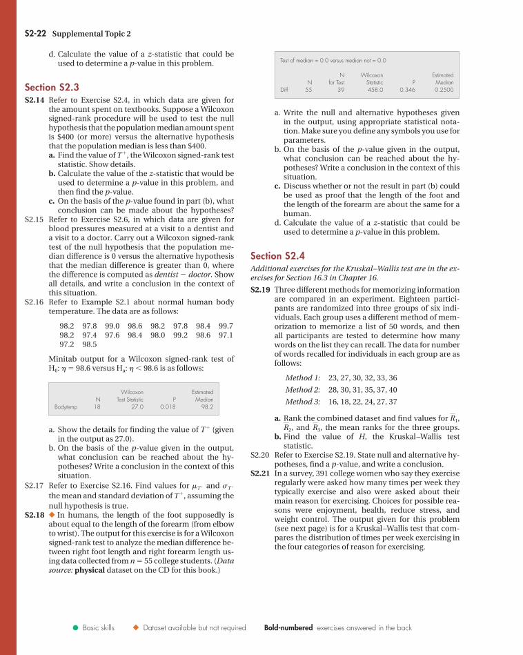
S2.18 � In humans, the length of the foot supposedly isabout equal to the length of the forearm (from elbowto wrist). The output for this exercise is for a Wilcoxonsigned-rank test to analyze the median difference be-tween right foot length and right forearm length us-ing data collected from n � 55 college students. (Datasource: physical dataset on the CD for this book.)

sT�mT�

Wilcoxon EstimatedN Test Statistic P Median

Bodytemp 18 27.0 0.018 98.2

a. Write the null and alternative hypotheses givenin the output, using appropriate statistical nota-tion. Make sure you define any symbols you use forparameters.


c. Discuss whether or not the result in part (b) couldbe used as proof that the length of the foot andthe length of the forearm are about the same for ahuman.

d. Calculate the value of a z-statistic that could beused to determine a p-value in this problem.

Section S2.4Additional exercises for the Kruskal–Wallis test are in the ex-ercises for Section 16.3 in Chapter 16.

S2.19 Three different methods for memorizing informationare compared in an experiment. Eighteen partici-pants are randomized into three groups of six indi-viduals. Each group uses a different method of mem-orization to memorize a list of 50 words, and thenall participants are tested to determine how manywords on the list they can recall. The data for numberof words recalled for individuals in each group are asfollows:

Method 1: 23, 27, 30, 32, 33, 36

Method 2: 28, 30, 31, 35, 37, 40

Method 3: 16, 18, 22, 24, 27, 37

a. Rank the combined dataset and find values for and the mean ranks for the three groups.

b. Find the value of H, the Kruskal–Wallis teststatistic.

S2.20 Refer to Exercise S2.19. State null and alternative hy-potheses, find a p-value, and write a conclusion.

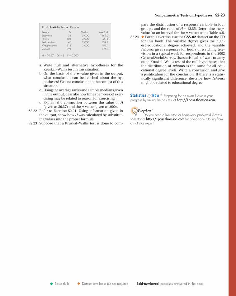
S2.21 In a survey, 391 college women who say they exerciseregularly were asked how many times per week theytypically exercise and also were asked about theirmain reason for exercising. Choices for possible rea-sons were enjoyment, health, reduce stress, andweight control. The output given for this problem(see next page) is for a Kruskal–Wallis test that com-pares the distribution of times per week exercising inthe four categories of reason for exercising.

R3,R2,R1,

Test of median = 0.0 versus median not = 0.0

N Wilcoxon EstimatedN for Test Statistic P Median

Diff 55 39 458.0 0.346 0.2500



S2-W3527 9/28/05 4:03 PM Page S2-22

pare the distribution of a response variable in fourgroups, and the value of H � 12.35. Determine the p-value (or an interval for the p-value) using Table A.5.

S2.24 � For this exercise, use the GSS-02 dataset on the CDfor this book. The variable degree gives the high-est educational degree achieved, and the variabletvhours gives responses for hours of watching tele-vision in a typical week for respondents in the 2002General Social Survey. Use statistical software to carryout a Kruskal–Wallis test of the null hypotheses thatthe distribution of tvhours is the same for all edu-cational degree levels. Write a conclusion and givea justification for the conclusion. If there is a statis-tically significant difference, describe how tvhoursmight be related to educational degree.

Preparing for an exam? Assess yourprogress by taking the post-test at http://1pass.thomson.com.

Do you need a live tutor for homework problems? AccessvMentor at http://1pass.thomson.com for one-on-one tutoring froma statistics expert.

a. Write null and alternative hypotheses for theKruskal–Wallis test in this situation.


c. Using the average ranks and sample medians givenin the output, describe how times per week of exer-cising may be related to reason for exercising.

d. Explain the connection between the value of H(given as 30.37) and the p-value (given as .000).

S2.22 Refer to Exercise S2.21. Using information given inthe output, show how H was calculated by substitut-ing values into the proper formula.

S2.23 Suppose that a Kruskal–Wallis test is done to com-

Kruskal–Wallis Test on Reason

Reason N Median Ave RankEnjoyment 31 5.000 282.2Health 101 3.000 200.4Reduce stress 48 2.000 139.2Weight control 211 3.000 194.1Overall 391 196.0

H = 30.37 DF = 3 P = 0.000



S2-W3527 9/28/05 4:03 PM Page S2-23

Click on the desired section below to position to that page. You may

Documents

Transcript of Click on the desired section below to position to that page. You may