An efficient rounding-off rule estimator:

Application to daily rainfall time series

Roberto Deidda1

Received 7 August 2006; revised 22 February 2007; accepted 7 June 2007; published 15 December 2007.

[1] An overview of problems and errors arising when fitting parametric distributions andapplying goodness of fit tests on samples containing roughly rounded off measurementsis first illustrated. The paper then presents the rounding-off rule estimator (RRE), anoriginal method that allows the estimation of the percentages of rainfall measurementsthat have been rounded at some potential resolutions. The efficiency of the RRE isevaluated using a wide set of samples drawn by different distributions and rounded offaccording to different rounding rules. Finally, the RRE is applied on 340 daily rainfall timeseries collected by the rain gauge network of the Sardinian Hydrological Survey (Italy).In most stations, results revealed the presence of significant percentages of roughlyrounded-off measurements, even at 1 and 5 mm resolutions, rather than at the standard0.1 or 0.2 mm discretization. The application of the proposed RRE may give importantsupport to perform quality data analyses, to assess and discriminate methods to fitparametric distributions on rounded-off samples, and to detect if and how the precision ofrecorded measurements might have changed in long time series used for climatic changestudies.

Citation: Deidda, R. (2007), An efficient rounding-off rule estimator: Application to daily rainfall time series, Water Resour. Res.,

43, W12405, doi:10.1029/2006WR005409.

1. Introduction

[2] The analysis of long time series of observations oftenrequires taking into account the different sampling rulesthroughout the considered period. This is a well knownproblem when dealing with paleoclimatic time series wherethe older data are usually estimated by indirect measurementof other variables or proxies, while the more recent data arerecorded by dedicated instruments. In these cases, series canbe easily split into records of old measures where data mayassume discrete and/or very approximate values (which areoften censored and sampled at irregular time intervals)and records of more recent measures collected at regularsampling times with appropriate resolutions to correctlydescribe the process of interest. To take into account theseand other kinds of inhomogeneities in the sampling of data,methods have been developed and widely applied [e.g., seeMartins and Stedinger, 2001; Brunetti et al., 2006, andreferences therein].[3] When dealing with time series recorded in the last

century, such as daily rainfall collected by rain gauges, oneexpects to analyze records with an appropriate resolution.For instance, the standard resolution of daily rainfall meas-urements taken by the Hydrological Surveys in Italy, andalso in many other countries, should be 0.1 or 0.2 mm/d.Unfortunately, as it will be shown in section 4 of this paper,a systematic analysis conducted on 340 time series collectedbetween 1922 and 1980 by the Hydrological Survey of the

Sardinia Region (Italy) revealed a different situation. Only33 series (i.e., less than 10% of the whole data set) werecorrectly recorded at the standard discretization of 0.1 or0.2 mm/d, while in most stations a lot of values wererounded off at larger resolutions, often at 1 or 5 mm/dand sometimes even at 10 mm/d. In 160 time series thepercentage of records rounded off at 5 mm resolution rangesbetween 10% to 40% of the whole record.[4] The reason of the presence of such roughly rounded-

off values should be searched in the way in which dailyrainfall depths were measured in the analyzed period. Tillthe 80s, in Italy, as in many other countries, rain gaugenetworks were set up mainly with two types of instruments:a lot of nonrecording standard rain gages (that require dailymanual measurement by an entrusted person) and veryfew recording gages (mainly tipping buckets that tracerainfall signals on weekly strip charts). Only after the 80s,rain gauge networks were progressively updated with theinstallation of automatically recording rain gauges that storerainfall information directly in memory chips and are oftenable to transmit, in real time, the rainfall evolution to acentral office.[5] Recording tipping bucket rain gauges have been

adopted since the beginning of the 1900s by the Italianand many other Hydrological Surveys. These devices tracevertical tips, each one corresponding to 0.2 mm rainfalldepth, in rotating strip charts. Daily rainfall depths are thenestimated on these paper charts by specialized staff, thustime series derived from these kind of stations are usuallycorrectly discretized at 0.2 mm resolution.[6] Anomalous percentages of roughly rounded-off

records are instead present in most time series collectedby nonrecording standard rain gauges. These devices

1Dipartimento di Ingegneria del Territorio, Universita di Cagliari,Cagliari, Italy.

Copyright 2007 by the American Geophysical Union.0043-1397/07/2006WR005409$09.00

W12405

WATER RESOURCES RESEARCH, VOL. 43, W12405, doi:10.1029/2006WR005409, 2007ClickHere

for

FullArticle

1 of 15

consist of a cylindrical collector above a funnel leading to areceiver. Italian and many other European standard gaugeshave a 0.1 m2 orifice [Tonini, 1959], thus 1 L of storedwater corresponds to 10 mm of rainfall depth. Dailymeasurements are then obtained by pouring the catch fromthe receiver into measuring glasses. Sardinian HydrologicalSurvey adopted three sizes of glasses: 1 L, 1/2 L, and 1 dLcapacity, corresponding to 10 mm, 5 mm, and 1 mm rainfalldepth respectively. A truncated measure of daily rainfalldepth (in millimeters) can be obtained by counting howmany times the 1-L glass can be fully filled, and then howmany times the water remaining in the last incompletelyfilled glass allows fully filling the 1/2-L and the 1-dLglasses. Finally, inserting a calibrated measuring stick inthe last incompletely filled 1-dL glass allows the estimationof how many tenths of millimeter should be added to theprevious measure. Thus the standard discretization of thesekinds of data should be 0.1 mm.[7] These very simple, but delicate, measurements were

not carried out by Hydrological Survey staff, but by peopleworking or living in places close to the rain gauge location.They were entrusted with the daily measuring operationsdescribed above, and had to annotate the number of fullyfilled glasses of each type, as well as the stick measure, onregisters that today remain the only information we haveabout rainfall occurred in the past. Annotations werethen converted by Hydrological Survey staff into dailyrainfall depths that were published in yearly reports (AnnaliIdrologici).[8] We suppose that the anomalous concentrations of

roughly rounded-off values may be attributed to thescarce devotion of these entrusted people to the delicatemeasuring operations required to estimate daily rainfalldepths. Rounded-off values at 5 mm resolution may bedue to the use of the first two glasses only. Instead,anomalous concentration of ties at multiples of 1 mm meansthat all the three glasses were used, but the final estimationby the stick was not carried out.[9] Standard discretization of 0.1 or 0.2 mm resolution,

usually prescribed for rainfall measurements, should be fineenough to allow parametric distributions to be accuratelyfitted without the need of applying estimation methodsfor discrete data (such as, e.g., the binned maximumlikelihood). Nevertheless, even the standard discretizationmay be a source of errors for some kind of statisticalanalysis, such as the moment scaling function estimation[Harris et al., 1997].[10] However, when significant percentages of records

are rounded off at resolutions larger than the standarddiscretization, as detected in many of the time seriesanalyzed here, even errors in fitting parametric distributionsand in applying goodness of fit tests become particularlyrelevant and cannot be disregarded, as described in section 2of this paper. The knowledge of the rounding-off rules, i.e.,the percentage of records rounded off at different resolu-tions, is fundamental to overcome some of these problems,such as the derivation of the proper percentage points forstatistical tests aimed at evaluating the goodness of fitteddistributions [Deidda and Puliga, 2006]. Nevertheless, theempirical determination of the rounding-off rules may be adifficult task when dealing with databases containing manystations, and, moreover, it may be affected by subjective

sensibility. Thus, in this paper, we develop an objectivestatistically based method to estimate the rounding-off rulesin any time series. The derivation of this rounding-off ruleestimator (RRE) is presented in Appendix A, while theperformances are evaluated and discussed in section 3.section 4 is devoted to show the results of a systematicapplication of the proposed estimator on 340 time series ofdaily rainfall depths in our database. In section 5, conclu-sions are drawn and potential applications of the RRE arebriefly discussed.

2. Undesirable Effects Arising With Rounded-offRecords

[11] The aim of this section is to highlight and commenton some undesirable effects arising in fitting parametricdistributions and applying goodness of fit tests on samplescontaining roughly rounded-off records. We refer to the realcases of two daily rainfall time series: the first one (recordedby station 007) is a badly discretized time series, since ahigh percentage of data were rounded off at 1 mm and 5 mmresolution, while the second one (recorded by station 235)is a quasi-perfect discrete time series with most valuesrounded at 0.1 or 0.2 mm. In the following, we will nameperfect discrete time series only those series containing allrecords rounded at 0.1 mm. In detail, the application of therounding-off rule estimator, derived in Appendix A,revealed that the 44-year-long time series recorded by thebad station 007 contains 37% of values rounded off at0.1 mm resolution, 24% rounded at 1 mm, and 39% ofvalues rounded at 5 mm. The same analysis performed onthe quasi-perfect time series (50 years long), retrieved bystation 235, determined that 85% of data were rounded at0.1 or 0.2 mm, while the remaining 15% were rounded at1 mm.

2.1. Fitting Parametric Distributions

[12] Time series of daily rainfall data usually contain zeroand non zero values. Thus several modeling approachesfirst separate rainy from not rainy data, and then separatelydeal with the distribution of rainfall occurrences (i.e., thesuccession of wet and dry periods) and the distribution ofrainfall values in rainy days. Often, all strictly positiverainfall data are then used to fit a distribution of rainyvalues. If this is the case, the following general equationF(x) can be assumed as cumulative distribution function(CDF) of rainy and not rainy values x on each time series:

F xð Þ ¼ 1� z0ð Þ þ z0F0 xð Þ x � 0 ð1Þ

where z0 = Pr{X > 0} represents the probability ofoccurrence of rainy days, while F0(x) = Pr{X � xjX > 0}is the CDF of only rainy values.[13] Nevertheless, it would be advisable to carefully

analyze the smallest record values before fitting F0(x) usingall strictly positive rainfall data. Indeed, distribution of verysmall values may be not clearly definite: small values maybe due to dew processes rather than being true rainfall, theremay be effects of subjective rounding and errors, and,whatever the cause may be, there are empirical evidencesthat small values often depart from the distribution ofhigher rainfall values. The generalized Pareto distribution[Pickands, 1975] explicitly requires to put a threshold on

2 of 15

W12405 DEIDDA: AN EFFICIENT ROUNDING-OFF RULE ESTIMATOR W12405

data and to infer parameter values only on records exceed-ing the threshold. Anyhow, it would be a good rule to applythe same approach whatever distribution is candidate todescribe daily rainfall, and to choose a threshold value thatallows the inferred distribution to be accepted, applying forinstance a goodness of fit test.[14] Adopting this last approach, once the threshold u has

been selected, we can fit a CDF Fu(y) on the (strictlypositive) exceedances y = x � u, where x is the originalsample of daily rainfall. The fitted distribution Fu(y)allows then to compute quantiles of daily rainfall (in therange x > u) as x = u + Fu

�1(P), where P = Pr{Y � yjY > 0} =Pr{X � xjX > u}, and Fu

�1 is the inverse function of Fu.[15] Let us consider the case that an estimation method

based on the simple moments (SM) or on the probabilityweighted moments (PWM) is applied to infer parametervalues of any distribution Fu(y) chosen as candidate formodeling the excesses y. If the chosen distribution maycorrectly describe only data exceeding a nonzero threshold u,moments or L moments have to be computed only on the(strictly positive) exceedances y = x � u. As an example, forthe two time series selected above, Figure 1 shows themean, the coefficient of variation CV and the L momentcoefficient of variation L-CVof the exceedances y computedfor left-censoring thresholds u ranging from 0 to 10 mm. Forthe badly discretized time series (left plots in Figure 1) wecan observe how the mean of excesses y decreases when uranges from 0 to 5 mm; for u = 5 mm there is a jump wherethe mean assumes again an high value; than the meandecreases again for u ranging from 5 to 10 mm. Althoughnot shown, the mean decreases with the same behavior ineach following 5-mm interval, while other jumps are local-ized at u = 10 mm, 15 mm, 20 mm, etc. Similar commentshold for CV and L-CV statistics computed on y for differentleft-censoring thresholds u, but the statistics are nowincreasing in each 5-mm interval of thresholds u. Therepetition of the described patterns are an effect of the largepercentage of values rounded at 5 mm resolution. Indeed, if

we look at moments and L moments computed on the quasi-perfect discrete time series (right plots in Figure 1) we canobserve a regular behavior for thresholds u larger thanabout 2 3 mm: mean increases linearly with u, whileCV and L-CV become nearly constant, and jumps onmultiples of 5 mm are not present any more. Looking morein detail, also in this case we can observe small jumpsrepeated for u multiples of 1 mm: they are due to thepresence of about 15% of values rounded off at 1 mmresolution. Anyhow, the spread remains very limited sincemost of data are anyway correctly discretized. Although notshown in Figure 1, similar behaviors can be observedcomputing higher moments and L moments that are neededto fit distributions with more than two parameters.[16] Using the sample moments or L moments shown in

Figure 1 to fit any one or two parameters distribution leadsto a consequent spread on the parameter estimates. As anexample, for the two considered time series, we show inFigure 2 the estimates of the parameters of the followinggeneralized Pareto distribution (GPD):

Fu x;au; xð Þ ¼ Pr X � xjX > uf g

¼1� 1þ x

x� u

au

� ��1=x

x 6¼ 0

1� exp � x� u

au

� �x ¼ 0:

8>>><>>>:

where x is the shape parameter, au the scale parameter,while u is the threshold value.[17] Although u is often referred to as ‘‘position’’ or

‘‘location’’ parameter, it cannot be considered as a truedistribution parameter. Indeed, it is used to left-censorsample x before fitting equation (2), and thus it should befixed a priori. This is also the reason why the maximumlikelihood (ML) estimation method does not allowto estimate u (indeed we cannot maximize a likelihoodfunction for a sample where some values may be excludedby the left-censoring threshold u itself), and why the SM

Figure 1. Simple moments and L moments of excess y over thresholds u: y = x � u, where x > u areleft-censored daily rainfall records. Mean m, coefficient of variation CV, and L moment coefficient ofvariation L-CV of y are plotted versus u for (left) station 007 and (right) station 235.

ð2Þ

W12405 DEIDDA: AN EFFICIENT ROUNDING-OFF RULE ESTIMATOR

3 of 15

W12405

and PWM methods require only the first two moments or Lmoments, computed on the excesses y, to estimate x and au.[18] In order to estimate the shape x and the scale au

parameters of the generalized Pareto distribution, weapplied the SM and PWM methods on the basis of theexpression reported by Hosking and Wallis [1987] andStedinger et al. [1993]. The ML estimates of the sameparameters were obtained by the optimized univariateapproach proposed by Grimshaw [1993]. Note that the signadopted for the shape parameter in the above referred worksis opposite with respect to equation (2).[19] The x parameter controls the tail behavior of the

distribution. For x = 0 the distribution has the ordinaryexponential form. For x > 0 the distribution has a long righttail, thus it is often referred to as ‘‘heavy tailed distribu-tion’’: in this case, simple moments of order greater than orequal to 1/x are degenerate, thus for x 1/2 mean andvariance do not degenerate and allow fitting equation (2)with the SM method. For x < 0 the distribution is shorttailed with an upper bound value (u � au/x).[20] The generalized Pareto distribution has a very

important property: if a sample can be reasonably consid-ered drawn by a GPD Fu0(x) with threshold u0 and param-eters x and au0, then the excesses above any other thresholdu > u0 should also follow the GPD in equation (2) with thesame shape parameter x and a scale parameter au given bythe following equation [Coles, 2001, p. 83]:

au ¼ au0 þ x u� u0ð Þ ð3Þ

[21] Thus, once GPD parameters x and au of Fu(x) inequation (2) are estimated on the excesses above anythreshold u > u0, equation (3) allows also to reparameterizea generalized Pareto distribution F0(x) that will be perfectlyoverlapping to the fitted Fu(x) for any x > u. Such adistribution F0(x) can be described by equation (2) with athreshold u = 0, the same x parameter estimated for Fu(x),

and a shape parameter a0 obtained for u0 = 0 by equation (3),which can be rewritten as

a0 ¼ au � xu ð4Þ

[22] The reparameterized distribution F0(x) is able todescribe all rainy values since it is defined for x > 0,although there may be departures from very small valuesx 2 (0, u0). Moreover, inserting F0(x) in equation (1) allowsmodeling in a simple way the whole rainfall process,including the rainy and not rainy occurrences. Finally, wehighlight that, in virtue of equation (4), both the x and a0

parameters should be constant if they are estimated fordistributions Fu(x) with any threshold u > u0.[23] Figure 2 shows the estimates of x and a0 obtained

by the simple moments (SM), the probability weightedmoments (PWM) and the maximum likelihood (ML)methods for thresholds u ranging form 0 to 10 mm. Leftplots of Figure 2 refer to the badly discretized time seriesand clearly show how the spread of moments and Lmoments observed in the left plots of Figure 1 reflect alsoon parameter estimates obtained by the SM and PWMmethods. Moreover, it is apparent that also the ML esti-mates, shown in the same plots, display a similar spread,revealing that also the ML estimation method is sensitive tothe presence of ties. The spread of the x estimates for station007 ranges from �0.3 to 0.3, with some differences amongthe considered fitting methods: it is clearly unlikely that byvarying the left-censoring threshold u the behavior of thefitted distribution may oscillate from a bounded type (x < 0)to an heavy tailed one (x > 0). As a matter of fact (as shownin Figure 8 discussed in section 4), the distribution of databelonging to station 007 is very close to an exponential one(x � 0). The oscillation of the distribution shape, when left-censoring data with different threshold values, is clearly anartificial effect that is driven by the large percentage ofvalues rounded off at 5 mm resolution.

Figure 2. Parameters x and a0 of the generalized Pareto distribution F0(x) in equation (2): SM, PWM,and LM estimates obtained using different thresholds u are compared. Shown are data from (left) station007 and (right) station 235.

4 of 15

W12405 DEIDDA: AN EFFICIENT ROUNDING-OFF RULE ESTIMATOR W12405

[24] Let us now look at the right plots of Figure 2, whichrefer to the quasi-perfect discrete time series. We canobserve that both the x and a0 estimates become nearlyconstant, as expected by theoretical arguments, for anythreshold larger then u0 � 2 3 mm. As already noticedin Figure 1, very small jumps are still present every 1 mm.Nevertheless, the spread of estimates remains very limitedbecause of the small percentage of values rounded at 1 mmas well as to the small rounding resolution itself.[25] The size of errors induced by fitting parametric

distributions to roughly rounded-off measurements is illus-trated in Figure 3. Empirical cumulative distribution func-tions of daily rainfall depths recorded by station 007 and235 are compared with the generalized Pareto distributionsfitted to left-censored samples with thresholds u in the range2.5 12.5 mm (the ML estimates displayed in Figure 2 areused). For the badly discretized time series (left plot inFigure 3), a wide spread of fitted distributions is apparent.Moreover, depending on the applied threshold, the 5-yearreturn period quantile provided by the fitted distributionmay be larger than the largest observed value in 44 years ofobservations! Conversely, distributions fitted on the quasi-perfect discrete time series (right plot in Figure 3) resultclose each other.

2.2. Goodness of Fit Tests

[26] Other undesirable effects arise when computinggoodness of fit statistics on rounded-off records. In fact,the presence of ties may change the distribution of teststatistics, thus using the percentage points derived byasymptotic distributions for continuous samples (usuallyavailable in tables of books and scientific papers) may leadto misinterpret the goodness of fit test results [Deidda andPuliga, 2006]. To clarify better this aspect, we focus on theW2 Cramer–von Mises and A2 Anderson-Darling statistics.Both are empirical distribution function (EDF) statisticssince they measure the discrepancy between the empiricaldistribution function and the tested cumulative distribution

function G(x), whose parameters may be known orunknown [Stephens, 1986]. For a sample of size n, W2

and A2 can be defined as

W 2 ¼ 1

12nþXni¼1

G xið Þ � 2i� 1

2n

� �2

ð5Þ

A2 ¼ �n�Xni¼1

2i� 1

nlog G xið Þð Þ þ log 1� G xnþ1�ið Þð Þ½ � ð6Þ

where xi are sample values arranged in increasing order,while G is the cumulative distribution function that will betested for fitting.[27] W2 and A2 statistics are often employed in goodness

of fit tests: first, equations (5) and (6) are evaluated usingsample data and the fitted distribution G, then the results arecompared with percentage points at a given confidencelevel. Examples of applications of these tests to evaluatethe goodness of fit of various distributions to hydrologicdata can be found in work by Ahmad et al. [1988], Clapsand Laio [2003], Choulakian and Stephens [2001], Dupuis[1999], and Laio [2004]. It is worthwhile to remark that thedistributions of EDF statistics, and thus also percentagepoints to be used in statistical tests, depend on the fittingdistribution G itself (e.g., distributions of W 2 and A2 forthe generalized extreme value and the GPD families aredifferent), on the shape of G, on the parameters of G to beestimated, on the parameter estimation method, and on thesample size.[28] Stephens [1986] provided percentage points of W 2

and A2 in case parameters of some widely used distributionsare estimated by the ML method, but the generalized Paretodistribution was not considered. Choulakian and Stephens[2001] studied asymptotic distributions of W 2 and A2

statistics in case equations (5) and (6) are evaluated on

Figure 3. Points (drawn using the Weibull plotting position) displaying the empirical distributionfunctions of daily rainfall depth collected by (left) station 007 and (right) station 235. Lines representfitted GPD Fu(x) in equation (2) for different thresholds u (values from 2.5 to 12.5 mm with increment of0.1 mm are used). Right vertical axes report some return periods T that were associated with exceedanceprobability P = 1 � 1/(365.25 T).

W12405 DEIDDA: AN EFFICIENT ROUNDING-OFF RULE ESTIMATOR

5 of 15

W12405

samples drawn by a generalized Pareto distribution, andonly one or both the scale and shape parameters areestimated by the ML method. They highlighted how EDFstatistics for GPD are only affected by the shape parameter(being invariant under scale changes) and provided tables ofpercentage points ofW2 and A2 at several significance levelsfor different x shape parameters.[29] In addition, we stress that percentage points of W 2

and A2 provided in tables and expressions within some ofthe above cited works were derived for the case of distri-butions G fitted on continuous samples. In case we aredealing with rounded measures, percentage points providedfor continuous samples cannot be applied anymore, sincethe presence of ties changes the distribution of the teststatistics. The Monte Carlo approach represents in thesecases the only way to correctly take into account sampleswith rounded records, once the rounding rule of the sampleitself is known. Moreover, the Monte Carlo approach takeseasily into account also the family and the shape of thefitting distribution, the estimation method, the parameters tobe estimated, and the sample size.[30] As an example, in Figure 4 the CDFs of test statistics

W 2 and A2 determined by Monte Carlo generations of10,000 GPD random samples are compared for the followingcases: case A, continuous samples (only computer roundoffdiscretization); case B, perfect discrete samples rounded offat the standard 0.1 mm resolution; case C, samples roundedoff at 0.1, 1 and 5 mm accordingly to the same rounding-offrule estimated for the badly discretized time series (station007), as reported at the beginning of the section. Allsamples have size 3000 and were drawn by a GPD F0(x)with parameters x = 0.02 and a0 = 8.7 mm, that allows agood fit on station 007 data to be obtained (see Figure 8).Both x and a0 parameters were first estimated by the MLmethod on each generated (continuous for case A orrounded for cases B and C) sample, then each fitted

distribution was used together with the same synthetic(and eventually rounded) sample in equations (5) and (6).The 10,000 values of W2 and A2 obtained in such a way areplotted in Figure 4.[31] It is apparent from Figure 4 that, even with a perfect

discrete sample, percentage points derived for continuoussamples need to be redetermined. The differences becomeeven more significant for samples with values roundedat larger resolutions, as it is the case of many time seriesin the analyzed database. A way to determine the correctpercentage points is illustrated in the same Figure 4. Indeed,once the confidence level has been chosen, quantiles orpercentage points can be obtained by (interpolation of) theempirical distribution of the test statistics obtained byMonte Carlo generations. Values obtained by Figure 4 forthe 90% confidence level (p value = 0.1) are reported inTable 1 and compared with percentage points provided by

Table 1. Dependence of A2 and W2 Percentage Points at 90%

Confidence Level on the Rounding-off Rule of the Samplea

W 2 A2

Asymptotic results (x = 0) 0.124 0.796Asymptotic results (x = 0.1) 0.116 0.766MC: case A continuous samples 0.121 0.789MC: case B perfect discrete samples 0.153 1.403MC: case C mixed rounded samples 5.411 31.215

aAsymptotic results are derived from Choulakian and Stephens [2001,Table 2] for GPD with shape parameters x = 0 and x = 0.1 and refer to thecase that both the unknown x and a0 parameters are estimated by the MLmethod. Monte Carlo (MC) results were obtained by applying the MLmethod on 10,000 GPD random samples of size 3000 generated withparameters x = 0.02 and a = 8.7 mm. MC results refer to the followingcases: case A, continuous samples; case B, perfect discrete samples (allrecords rounded at 0.1 mm); and case C, mixed rounded samples with thesame rounding-off rule estimated on station 007. Percentage points for MCexperiments are obtained by quantiles of CDFs plotted in Figure 4.

Figure 4. CDFs of test statistics (left) W2 and (right) A2 determined by Monte Carlo generations of10,000 GPD random samples with parameters x = 0.02 and a = 8.7 mm. Solid line (case A) refers tocontinuous samples; dashed line (case B) refers to perfect discrete samples, rounded off at resolution0.1 mm; and dotted line (case C) is traced for samples rounded off with the same rounding rule estimatedon station 007, i.e., 37% at resolution 0.1 mm, 24% at resolution 1 mm, and 39% at resolution 5 mm.

6 of 15

W12405 DEIDDA: AN EFFICIENT ROUNDING-OFF RULE ESTIMATOR W12405

Choulakian and Stephens [2001, Table 2]. Table 1 showsthat percentage points for continuous samples (case A) arevery close to the linear interpolations of values provided byChoulakian and Stephens [2001] for x = 0 and x = 0.1;percentage points for perfect discrete samples (case B)become about 1.5 2 times the values for continuous case;and for samples rounded as station 007 records, percentagepoints become about 50 times greater than those valid forcontinuous samples. This example clearly shows howapplying goodness of fit tests without knowing how theanalyzed sample has been rounded off would certainly bringwrong conclusions. Indeed, only once the rounding-off rulesare estimated, the proper percentage points for applicationof statistical tests can be derived.

2.3. Final Remarks

[32] In this section we have highlighted, with the aid ofsome examples, how the presence of rounded-off recordsmay lead to undesirable and sometimes unexpected prob-lems when fitting parametric distributions and/or whenapplying goodness of fit tests. Although we considered onlythe generalized Pareto distributions, we stress that similarproblems arise also for any other continuous parametricdistribution, with one, two or more parameters. The follow-ing sections develop a methodology to estimate the round-ing-off rules from sample data. The knowledge of thepercentages of rounded-off values is necessarily the firststep to assess the best approach to estimate parameters ofparametric distributions, and to determine the percentagepoints for goodness of fit test correctly accounting for therounding of the sample.

3. Description and Performances of theRounding-off Rule Estimator

[33] The aim of this section is to briefly describe therounding-off rule estimator (RRE), whose derivation isprovided in Appendix A together with some details fornumerical implementation, and to evaluate the perform-ances of the estimator on synthetic samples that may beconsidered representative of daily rainfall time series.[34] The RRE provides the estimation of the percentages

of measurements rounded off at different resolutions withina given sample. It requires only a preliminary exploration ofthe data set in order to detect the r potential rounding-offresolutions D = {D j: j = 1,� � �,r}. This aim can be easilypursued by visual inspection of the empirical cumulativedistribution functions and frequency histograms, looking foranomalous recurrent ties. For instance, an exploration in the

data set analyzed in this paper revealed that recorded valuesmay have been rounded off at the following resolutions:

D ¼ 0:1; 0:2; 0:5; 1; 5½ �mm ð7Þ

[35] Then the RRE application requires to solve the setof linear algebraic equations (equation (A1)), given inAppendix A, where the matrix A of known coefficientscan be univocally determined once the vector D is defined.The solution of this set of equations is finally used inequation (A7), provided in Appendix A as well, to estimatethe probability P(D = Dj) that a value has been rounded offat each resolution D j, for j = 1,� � �,r.[36] Before applying the rounding-off rule estimator on

observed data (as exemplified in section 4, where wediscuss the results obtained by a systematic application ofthe RRE on a wide database of daily rainfall time series), itis essential to evaluate errors and performances of theestimator on synthetic series where we know a priori therounding-off rule. Thus, in subsection 3.1, we present apreliminary analysis of our data set aimed at identifyingreliable probability distributions of daily rainfall timeseries, while in Subsection 3.2 we discuss the setting oftest cases to evaluate the RRE performances, that are thensummarized in subsection 3.3.

3.1. Reliable Probability Distributions for RREPerformances Evaluation

[37] We assume that rainy values can be considereddrawn by a generalized Pareto distribution F0(x), describedby equation (2) with threshold u = 0. We assume also that,once F0(x) has been fitted and the probability of rainy daysz0 has been estimated, equation (1) is able to describe thewhole distribution of rainy and not rainy daily values. Westress that although equation (2) can often satisfactorily fitdaily rainfall data only adopting a non zero threshold u(generally a few millimeters may be enough), once au hasbeen estimated for any given threshold u, equation (4)allows to reparameterize equation (2) in order to obtainF0(x). In such a way, equation (1) not only gives a verysimple representation of rainy and not rainy values, butalso perfectly overlaps the GPD fitted on data exceedinga reliable threshold u. Certainly, there may be a littledeparture between equation (1) and the empirical distribu-tion of observed data in the range (0, u), but this does notaffect the finding of this section.[38] There are many reasons to assume rainfall depths

distributed as a GPD. Indeed, several studies have provedthat GPD is able to correctly fit rainfall depths at daily or

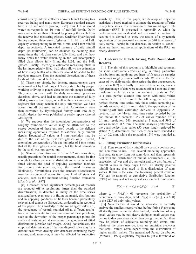
Table 2. Summary of the Rounding-off Rules P(D) and RRE Performances in All the Groups of Tests Considereda

Group D 0.1 m 0.2 m 0.5 m 1.0 m 5.0 m

Maximum Bias Maximum RMSE

N = 700 N = 3000 N = 700 N = 3000

A P(D) 0.4 0.1 0.1 0.1 0.3 0.018 0.018 0.042 0.023B P(D) 0.1 0.2 0.3 0.3 0.1 0.028 0.027 0.046 0.032C P(D) 0.2 0.2 0.2 0.2 0.2 0.023 0.022 0.038 0.027D P(D) 1 0 0 0 0 0.022 0.012 0.038 0.018E P(D) 0.5 0.2 0.3 0.004 0.004 0.022 0.011F P(D) 0.5 0.2 0.3 0.023 0.023 0.045 0.030

aIn the last four columns, the maximum RMSE and absolute bias among all Djs and all considered couples of (a, x) for parent distributions are reported.

W12405 DEIDDA: AN EFFICIENT ROUNDING-OFF RULE ESTIMATOR

7 of 15

W12405

smaller scales [see, e.g., Cameron et al., 2000; Coles et al.,2003; De Michele and Salvadori, 2005; Fitzgerald, 1989;Madsen et al., 2002; Salvadori and De Michele, 2001; VanMontfort and Witter, 1986]. Recently, Deidda and Puliga[2006] also gave evidence, using L moment ratio diagram[Hosking, 1990], that GPD is the best candidate to be theparent distribution of daily rainfall time series analyzedhere. Moreover, besides the above reasons, the GPD familyis particularly suitable for the scope of this section. IndeedF0(x) provided by equation (2) can easily represent datadistributions with different shapes and different scales, justchanging the x and a0 parameters, allowing the evaluationof the performances of the estimator in very differentconditions.[39] In order to reduce the estimation variance, parame-

ters x and a0 were estimated for the 200 longest time seriesof daily rainfall, each more than 40 years long. Moreover, todeal with the spread of estimates (x, a0) in stations withrounded data (as shown in Figure 2), the median valuesof the estimates for thresholds u ranging from 2.5 mm to12.5 mm were adopted. Figure 5 shows the couplesof parameters (x, a0) determined in such a way for the200 time series. For most stations, the generalized Paretodistributions F0(x), drawn adopting these couples of param-eters, appeared, at a visual inspection, very close to theempirical distribution functions. The aspects related toparameter estimation on samples containing rounded-offvalues would certainly deserve to be better deepened (e.g.,some of the adopted estimates would benefit from furtherrefinements), but this matter goes beyond the scope of thispaper. Here we use estimates (x, a0) presented in Figure 5only with the aim to evaluate the performances of the RREfor all the possible distributions of daily rainfall time seriesin our database.[40] As far as the last free parameter is concerned, i.e., z0

in equation (1), we found that in most stations the proba-

bility of rainy days is slightly larger than 20%, with a smallspread around this value.

3.2. Test Cases for RRE Performances Evaluation

[41] On the basis of results presented in subsection 3.1,we evaluated the performances of the RRE on samplesdrawn by generalized Pareto distributions F0(x) with shapeparameter x in the range from �0.15 to 0.35, and the scaleparameter a0 ranging from 5 to 15 mm. Moreover, samplesize N = 700 and N = 3000 were taken into account, sincethese lengths are representative of daily rainfall time seriesabout 10 years and 40 years long with a probability of rainz0 � 20%.[42] All test were performed in the following way. For

each couple (x, a0) in the ranges given above, we generatedS = 10,000 GPD random samples of size 700 and 3000, andthen we rounded-off data according to the rounding-off ruleP(D) chosen for the test. Finally we applied the RRE oneach rounded sample and evaluated the bias and the rootmean square error (RMSE) of the estimated probability ofeach rounding resolution Dj:

Bias P Dj

� �¼ 1

S

XSs¼1

Ps Dj

� � P Dj

� �

RMSE P Dj

� �¼

ffiffiffiffiffiffiffiffiffiffiffiffiffiffiffiffiffiffiffiffiffiffiffiffiffiffiffiffiffiffiffiffiffiffiffiffiffiffiffiffiffiffiffiffiffiffiffiffiffiffi1

S

XSs¼1

Ps Dj

� � P Dj

� �2vuut ð8Þ

where Ps(Dj) is the estimate, on the sth synthetic series, ofthe probability that records have been rounded off atresolution Dj, while P(Dj) is the probability really used toround off Monte Carlo samples at resolution Dj.[43] Performances of the RRE were evaluated for differ-

ent vectors of rounding-off resolutions D and associatedprobabilities P(D), that are reported in Table 2, where labelsA, B, C, D, E and F identify each couple D, P(D) used asrounding rule. In such a way we analyzed the performancesof the RRE for different rounding-off rules and for allpossible distributions of rainfall data. Examples of theRRE performances evaluated by equation (8) on eachrounding-off resolution Dj are presented in Tables 3 and 4.[44] In detail, for group A, B, C and D the RRE was

tested for the five-element vector of potential rounding

Figure 5. Parameters x and a0 of the generalized Paretodistribution F0(x) in equation (2), with u = 0, estimated from200 daily rainfall time series collected by the rain gaugenetwork of the Sardinian Hydrological Survey. Theobservation period is longer than 40 years for all consideredseries.

Table 3. Evaluation of Performances of the Rounding-off Rule

Estimator on S = 10,000 Samples Drawn by an Exponential

Distribution (x = 0) With Scale Parameter a0 = 10 mm and Then

Rounded off According to the Rounding-off Rule of Group A

D 0.1 mm 0.2 mm 0.5 mm 1 mm 5 mm

Rounding-off Rule Adopted for Group of Tests AP(D) 0.4 0.1 0.1 0.1 0.3

RRE Performances for Sample Size N = 3000Mean[P(D)] 0.402 0.101 0.091 0.105 0.301Bias[P(D)] 0.002 0.001 �0.009 0.005 0.001RMSE[P(D)] 0.019 0.016 0.015 0.014 0.011

RRE Performances for Sample Size N = 700Mean[P(D)] 0.402 0.100 0.092 0.105 0.301Bias[P(D)] 0.002 0.000 �0.008 0.005 0.001RMSE[P(D)] 0.039 0.034 0.027 0.027 0.022

8 of 15

W12405 DEIDDA: AN EFFICIENT ROUNDING-OFF RULE ESTIMATOR W12405

resolutions defined in equation (7). Thus, according toequation (A3), the matrix of probabilities aij becomes

A ¼

1 1 1 1 1

1

21

1

21 1

1

5

1

51 1 1

1

10

1

5

1

21 1

1

50

1

25

1

10

1

51

2666666666666664

3777777777777775

ð9Þ

[45] To understand better the meaning of probabilities inequation (A3), let us look at the values of the above matrixA. The first row contains the probabilities a1,js that thevalues rounded off at resolutions Djs provided in equation(7) might be multiples of 0.1 mm (D1). Thus the rowcontains only ones, since whatever discretization Dj is used,the rounded value is certainly a multiple of 0.1 mm. Thesecond row contains probabilities a2,js that the valuesrounded off at resolutions Djs might be multiples of0.2 mm (D2). Thus a2,1 = 1/2 means that we expect thatonly one half of values rounded off at resolution 0.1 mmwill be multiples of 0.2 mm; obviously a2,2 = 1; whilemeasurements rounded off with resolution 0.5 mm (D3) willbe multiples of 0.2 mm only when they take the values1 mm, 2 mm, 3 mm, etc., thus a2,3 = 1/2. Conversely, a3,2is equal to 1/5 since we expect that only one fifth ofmeasurements rounded off with resolution 0.2 mm aremultiples of 0.5 mm (this happens again when roundedmeasurements take the values 1 mm, 2 mm, 3 mm, etc.).Similar considerations hold also for the other coefficients.[46] Groups of tests A, B, C and D differ only for the

vector of probabilities P(D) used to round data at resolu-tions D provided in equation (7), as shown in Table 2.In group A, most data are rounded off at the smallest (D1 =0.1 mm) and largest resolutions (D5 = 5 mm). In group B,most data are rounded off at the inner and close resolutionsD3 = 0.5 mm and D4 = 1 mm. In group C, data are roundedoff with equiprobable rule. In group D, all data are rounded

off at the smallest resolution D1 = 0.1 mm (perfect discretesample).[47] Groups of tests E and F are instead aimed at showing

how the performances of RRE increase when the numberof potential resolutions decreases. For group E the vectorD = [0.1, 1, 5] mm has been used, while D = [0.1, 0.2, 0.5]mm was used for group F. The probability of rounding atsmallest, medium and largest resolution is the same for bothgroup of tests: P(D) = [50%, 20%, 30%].[48] Matrices A for test E and F become, respectively,

AE ¼

1 1 1

1

101 1

1

50

1

51

2666664

3777775; AF ¼

1 1 1

1

21

1

2

1

5

1

51

2666664

3777775

ð10Þ

[49] Tests of group D deserve a special comment sincethey were aimed at evaluating the size of false roundingdetections that may be induced by equation (A7) in casesRRE is applied to estimate probabilities of rounding atresolutions D, but sample values are rounded off only at asubset of resolutions. We chose the most critical case inwhich we are dealing with perfect discrete samples whereall values are rounded at resolution 0.1 mm, but the RRE isapplied with the vector of resolutions D provided inequation (7). An example of test results is presented inTable 4 for samples drawn by an exponential distribution(x = 0) with scale parameter a0 = 10 mm. If we look atresults for Dj 6¼ 0.1 mm, it is apparent from Table 4 thatRRE may provide probabilities different from zero forresolutions not used to round off data. Nevertheless, theerrors on probabilities of rounding at resolutions Dj 6¼0.1 mm, erroneously detected by the RRE, are still small:absolute values of bias and RMSE remain lower than 1%and 2% respectively for sample sizeN = 3000, correspondingto about 40-year-long series, and increase only to valueslower than 2% and 4% respectively for shorter series (N =700, corresponding to about 10-year-long series). We high-light also that owing to equation (A7), the size of theunderestimation of the probability of rounding at resolution0.1 mm is equal to the sum of probabilities estimated forrounding resolutions Dj 6¼ 0.1 mm. Since the aim of thisgroup of tests was to evaluate the size of false detection, themaximum absolute bias and the maximum RMSE weredetermined only among Dj 6¼ 0.1 mm.

3.3. Discussion of RRE Performances

[50] For the sake of synthesis in presenting results of thewide amount of cases considered in the tests, Table 2reports, for each group of test, only the maximum absolutevalue of the bias and the maximum RMSE among all theconsidered Dj and all the distributions F0(x) drawn with thedifferent couples of considered parameters (x, a0).[51] In Table 2 we can observe that the overall perform-

ances of RRE are generally very good, although there is aslight worsening when data are rounded at very closeresolutions, as in groups B and F. However, we want tostress here that our major interest is mainly addressed todetect rounding rules when data have been rounded at farand significantly different resolutions. Indeed, in these casesthe rounded values exert the larger statistical impact when

Table 4. Same as Table 3 but Here Samples Are Rounded off

According to the Rounding-off Rule of Group Da

D 0.1 mm 0.2 mm 0.5 mm 1 mm 5 mm

Rounding-off Rule Adopted for Group of Tests DP(D) 1 0 0 0 0

RRE Performances for Sample Size N = 3000Mean[P(D)] 0.980 0.009 0.002 0.007 0.001Bias[P(D)] �0.020 0.009 0.002 0.007 0.001RMSE[P(D)] 0.024 0.016 0.005 0.010 0.002

RRE Performances for Sample Size N = 700Mean[P(D)] 0.960 0.019 0.007 0.011 0.002Bias[P(D)] �0.040 0.019 0.007 0.011 0.002RMSE[P(D)] 0.050 0.034 0.016 0.017 0.004

aPerfect discrete samples: All records are rounded off at resolution0.1 mm.

W12405 DEIDDA: AN EFFICIENT ROUNDING-OFF RULE ESTIMATOR

9 of 15

W12405

fitting parametric distributions, or when applying testsbased on goodness of fit statistics, as shown in section 2.An example can better clarify this point. First, let usconsider a time series where all data were rounded at closeresolutions, for instance half and half at 0.1 mm and 0.2 mm.In this case, there is certainly a worsening of the perfor-mance (although bias and RMSE do not exceed fewpercentage points), nevertheless, we have less interest indiscriminating the percentage of data rounded at the twopossible resolutions: for instance, distributions of test sta-tistics, as those shown in Figure 4, do not significantlychange if RRE provides percentages of rounding at reso-lutions 0.1 mm and 0.2 mm slightly different from 50% and50% (note that RRE errors are anyhow lower than fewpercentage points). Conversely, if we look at a sample withvalues rounded at very far resolutions, for instance 0.1 mm

and 5 mm, there is a greater interest in discriminating thepercentage of roundings at the two resolutions, and in thiscase the RRE becomes even more efficient (as proved bygroups of tests A and E).[52] In conclusion, a general good efficiency of the RRE

has been verified in all the considered groups of tests:results can be summarized as follows. For the five-resolu-tion vector D, the maximum RMSE is about 2–3% for40-year-long time series (N = 3000) and only increases toabout 4% for 10-year-long time series (N = 700), while themaximum absolute value of the bias is around 2%. Consid-ering the most interesting case (group E) for the three-resolution vectors D, the maximum RMSE resulted about1% for 40-year-long time series (N = 3000) and about 2%for 10-year-long time series (N = 700), while the maximum

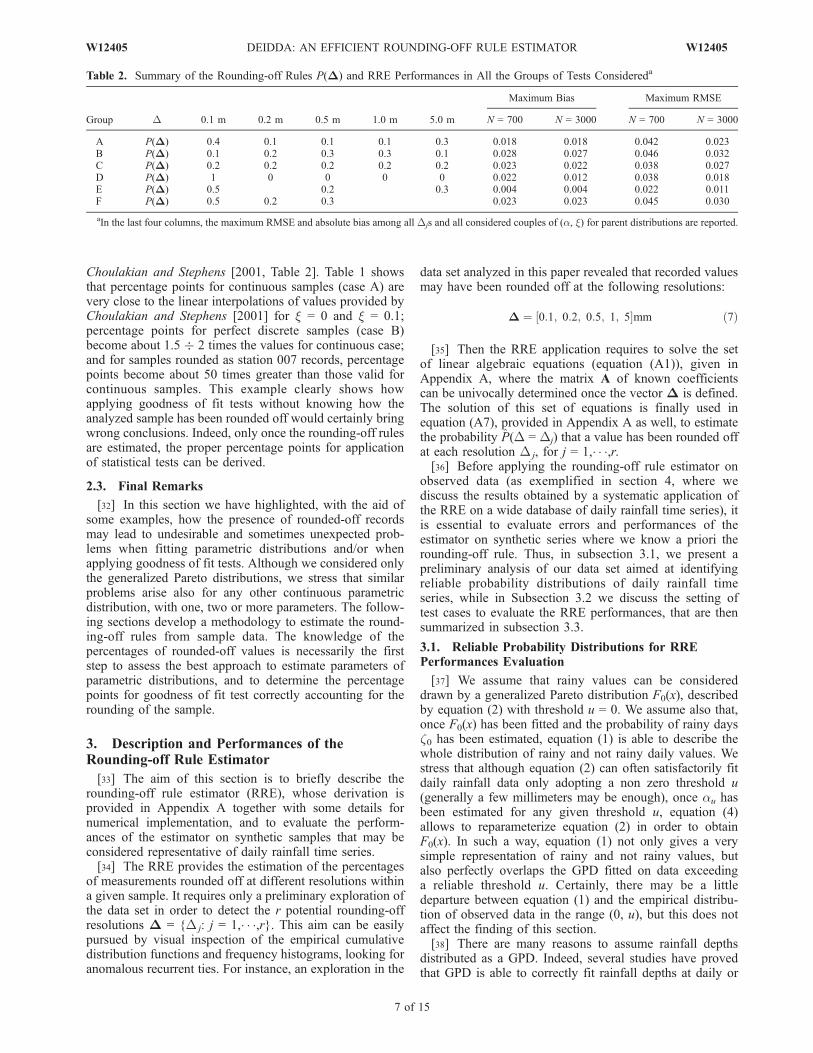
Figure 6. Results of the RRE on 340 daily rainfall time series that are more than 10 years long. For eachseries, rounding probabilities were first determined for resolutions D = [0.1, 0.2, 0.5, 1, 5] mm and thenwere recomputed only for those Dls for which P(Dl) > 10% resulted in order to exclude false detections.(a) Histogram classifying stations on the probability that measurements have been rounded at the smallestresolution D = 0.1 mm. (b) Histogram based on the probability that measurements have been rounded atD = 0.1 mm or D = 0.2. (c) Histogram based on the probability that measurements have been rounded atresolution D = 0.5 mm or smaller. (d) Histogram based on the probability that measurements have beenrounded at resolution D = 1 mm or smaller: Only 180 time series count more than 90% of data roundedoff at resolutions smaller than or equal to 1 mm; consequently, 160 series have more than 10% of recordsrounded off at larger resolutions (see Figure 7 for details).

10 of 15

W12405 DEIDDA: AN EFFICIENT ROUNDING-OFF RULE ESTIMATOR W12405

absolute value of the bias is less than 0.5% irrespective ofthe sample size.

4. RRE Application on Daily Rainfall Data

[53] The rounding-off rule estimator, described in Appen-dix A and tested in section 3, proved to be very efficienteven with small samples. Thus we applied it on the 340daily rainfall time series with more than 10 years of records,which were collected by the Hydrological Survey of theSardinia Region (Italy) from 1922 to 1980. Among these340 series, 200 ones count more than 40-year records andwere already used to produce Figure 5.[54] On each time series, the application has been per-

formed in two steps. At the first step the RRE has beenapplied to estimate the probabilities of rounding at resolu-tionsD = [0.1, 0.2, 0.5, 1, 5] mm. At a second step the RREhas been applied again only for those resolutions Dls forwhich resulted P(Dl) > 10%. On the basis of the resultsobtained for group of tests D, discussed in section 3, we arequite confident to exclude, in such a way, the chance toestimate non zero probabilities for unused rounding-offresolutions. Moreover, we obtain a secondary advantagesince reducing the size of vector D increases the efficiencyof the RRE.[55] Results of the RRE obtained for the 340 time series

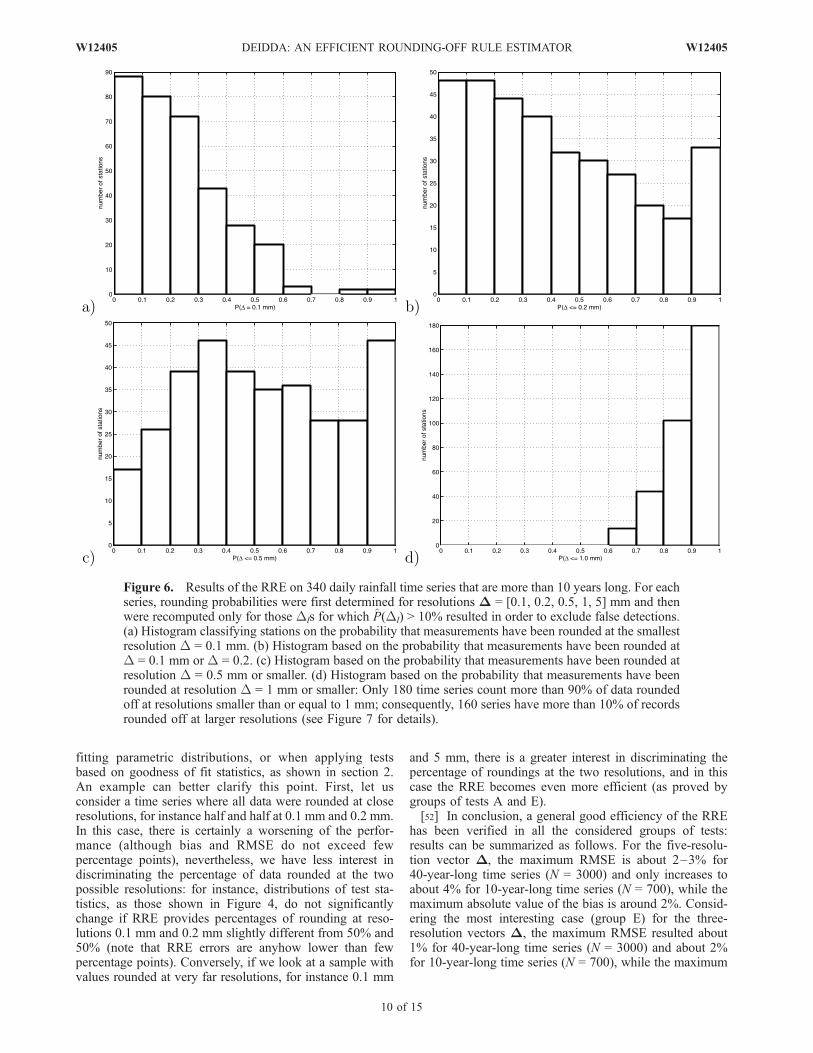
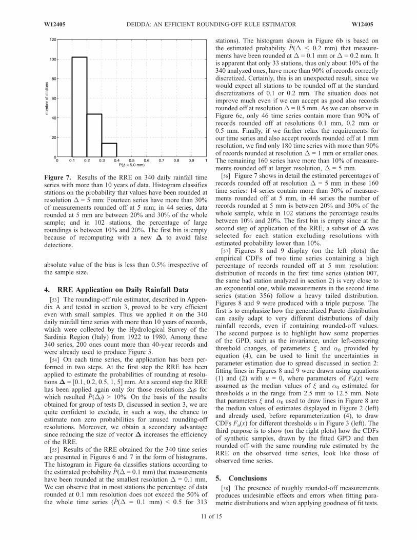
are presented in Figures 6 and 7 in the form of histograms.The histogram in Figure 6a classifies stations according tothe estimated probability P(D = 0.1 mm) that measurementshave been rounded at the smallest resolution D = 0.1 mm.We can observe that in most stations the percentage of datarounded at 0.1 mm resolution does not exceed the 50% ofthe whole time series (P(D = 0.1 mm) < 0.5 for 313

stations). The histogram shown in Figure 6b is based onthe estimated probability P(D � 0.2 mm) that measure-ments have been rounded at D = 0.1 mm or D = 0.2 mm. Itis apparent that only 33 stations, thus only about 10% of the340 analyzed ones, have more than 90% of records correctlydiscretized. Certainly, this is an unexpected result, since wewould expect all stations to be rounded off at the standarddiscretizations of 0.1 or 0.2 mm. The situation does notimprove much even if we can accept as good also recordsrounded off at resolution D = 0.5 mm. As we can observe inFigure 6c, only 46 time series contain more than 90% ofrecords rounded off at resolutions 0.1 mm, 0.2 mm or0.5 mm. Finally, if we further relax the requirements forour time series and also accept records rounded off at 1 mmresolution, we find only 180 time series with more than 90%of records rounded at resolution D = 1 mm or smaller ones.The remaining 160 series have more than 10% of measure-ments rounded off at larger resolution, D = 5 mm.[56] Figure 7 shows in detail the estimated percentages of

records rounded off at resolution D = 5 mm in these 160time series: 14 series contain more than 30% of measure-ments rounded off at 5 mm, in 44 series the number ofrecords rounded at 5 mm is between 20% and 30% of thewhole sample, while in 102 stations the percentage resultsbetween 10% and 20%. The first bin is empty since at thesecond step of application of the RRE, a subset of D wasselected for each station excluding resolutions withestimated probability lower than 10%.[57] Figures 8 and 9 display (on the left plots) the

empirical CDFs of two time series containing a highpercentage of records rounded off at 5 mm resolution:distribution of records in the first time series (station 007,the same bad station analyzed in section 2) is very close toan exponential one, while measurements in the second timeseries (station 356) follow a heavy tailed distribution.Figures 8 and 9 were produced with a triple purpose. Thefirst is to emphasize how the generalized Pareto distributioncan easily adapt to very different distributions of dailyrainfall records, even if containing rounded-off values.The second purpose is to highlight how some propertiesof the GPD, such as the invariance, under left-censoringthreshold changes, of parameters x and a0 provided byequation (4), can be used to limit the uncertainties inparameter estimation due to spread discussed in section 2:fitting lines in Figures 8 and 9 were drawn using equations(1) and (2) with u = 0, where parameters of F0(x) wereassumed as the median values of x and a0 estimated forthresholds u in the range from 2.5 mm to 12.5 mm. Notethat parameters x and a0 used to draw lines in Figure 8 arethe median values of estimates displayed in Figure 2 (left)and already used, before reparameterization (4), to drawCDFs Fu(x) for different thresholds u in Figure 3 (left). Thethird purpose is to show (on the right plots) how the CDFsof synthetic samples, drawn by the fitted GPD and thenrounded off with the same rounding rule estimated by theRRE on the observed time series, look like those ofobserved time series.

5. Conclusions

[58] The presence of roughly rounded-off measurementsproduces undesirable effects and errors when fitting para-metric distributions and when applying goodness of fit tests.

Figure 7. Results of the RRE on 340 daily rainfall timeseries with more than 10 years of data. Histogram classifiesstations on the probability that values have been rounded atresolution D = 5 mm: Fourteen series have more than 30%of measurements rounded off at 5 mm; in 44 series, datarounded at 5 mm are between 20% and 30% of the wholesample; and in 102 stations, the percentage of largeroundings is between 10% and 20%. The first bin is emptybecause of recomputing with a new D to avoid falsedetections.

W12405 DEIDDA: AN EFFICIENT ROUNDING-OFF RULE ESTIMATOR

11 of 15

W12405

Assuming the generalized Pareto distribution (GPD) asparent distribution of daily rainfall records, we have shownhow roughly rounded-off values in the analyzed samplesmay cause wide spreads of parameters estimates when somecommon and widely adopted estimation methods are ap-plied (the simple moments, the probability weightedmoments and the maximum likelihood estimators wereconsidered here). Although we only showed results for theGPD, we highlight that similar problems arise even if anyother continuous parametric distribution is candidate tomodel left-censored samples. Indeed, the spread of param-eters estimates is driven by the spread of the samplestatistics computed on the excesses above left-censoringthresholds. Moreover, the presence of rounded-off valuesmay also change the distribution of goodness of fit statistics,as shown for the Cramer–von Mises and the Anderson-Darling ones. Thus the right determination of percentagepoints for a correct application of statistical tests requires

the knowledge of the rounding-off rule of the analyzedsample.[59] The paper presents an original objective statistically

based method that allows the estimation of the percentagesof measurements that were rounded off at some predeter-mined resolutions. The efficiency of the rounding-off ruleestimator (RRE) has been proved to be high on differentdistributions (that can reliably describe the variety of dailyrainfall distributions in the analyzed data set) and differentrounding-off rules. A wide set of tests showed that for40-year-long time series the maximum RMSE of probabil-ities estimated on 5 potential rounding-off resolutions isabout 2–3%, and that it becomes lower than 1% whenconsidering 3 potential rounding-off resolutions. The effi-ciency remains good also for shorter time series. Indeed,considering 10-year-long time series the maximum RMSEincrease only to 4% and 2% for probabilities estimatedrespectively on 5 and 3 potential rounding-off resolutions.

Figure 8. GPD mixed with zeros according to equation (1) with parameters x = 0.02, a0 = 8.66 mm,and z0 = 21% (solid line). (left) Empirical CDFs of daily rainfall data collected by station 007 (circles).(right) Empirical CDFs of a synthetic sample drawn by a GPD with the parameters given above androunded off with rule D = [0.1, 1, 5], P(D) = [37%, 24%, 39%] (circles). (top) Plots in semi-log scale tohighlight the tail behavior. (bottom) Zoom of smaller values.

12 of 15

W12405 DEIDDA: AN EFFICIENT ROUNDING-OFF RULE ESTIMATOR W12405

[60] The RRE has been systematically applied to estimatethe rounding-off rules on 340 time series of daily rainfallrecords collected by the rain gauge network of the Hydro-logical Survey of the Sardinian Region (Italy). Resultsrevealed that most series contain significant percentagesof values rounded off at very large resolutions, even 1 mmand 5 mm, rather than being discretized at the standard 0.1or 0.2 mm resolution. The reasons for the presence ofanomalous tie concentrations at these resolutions werediscussed in the Introduction of the paper. We believe thatsimilar problems might also have happened in measuringrainfall depths in other rain gage networks, and thus theproposed rounding-off rule estimator represents a veryuseful method to evaluate the goodness of records also inother data sets.[61] In order to choose reliable estimates of GPD param-

eters, despite the large spreads due to the presence ofrounded values, we adopted the median values of parame-

ters estimated for different thresholds. In such a way,acceptable fit in most time series was obtained, as in theexamples shown in Figures 8 and 9. Nevertheless, therewere a few time series where, even adopting the medianvalues among multiple thresholds estimates, the fitted GPDsdid not perfectly describe the empirical distributions. Thusthe assessment of the best approach for parameter estima-tion on roughly discretized samples certainly deserves to bedeepened in forthcoming research activities, and the round-ing-off rule estimator may give an important support forthese tasks.[62] Finally, over the last years there has been an increas-

ing interest in assessing possible climate change on the basisnot only of meteorological scenarios, but also by theanalysis of long rainfall time series (e.g., some analyseson Italian daily rainfall time series has been performed byBrunetti et al. [2001a, 2001b, 2006] and Cislaghi et al.[2005]). The good performances demonstrated by the

Figure 9. GPD mixed with zeros according to equation (1) with parameters x = 0.28, a0 = 6.80 mm,and z0 = 23% (solid line). (left) Empirical CDFs of daily rainfall data collected by station 356 (circles).(right) Empirical CDFs of a synthetic sample drawn by a GPD with the parameters given above androunded off with rule D = [0.1, 0.5, 1, 5], P(D) = [31%, 11%, 31%, 27%] (circles). (top) Plots in semi-log scale to highlight the tail behavior. (bottom) Zoom of smaller values.

W12405 DEIDDA: AN EFFICIENT ROUNDING-OFF RULE ESTIMATOR

13 of 15

W12405

rounding-off rule estimator, even in the case of short timeseries (10 years long), make it an important analysis methodto support these kind of studies. In drawing conclusions inthis delicate subject, as well as in performing quality controland homogenizing procedures, the chance that the precisionof measurements and the rounding-off rules have changedduring the analyzed periods is certainly an important aspectto evaluate. Indeed, as we have shown, the rounding processmay affect the inference of distributions and may also alterthe percentage of recorded rainy days.

Appendix A: Rounding-off Rule Estimator (RRE)

[63] LetD = {Dl: l = 1,� � �,r} be the vector containing ther potential rounding-off resolutions of the data. Estimates ofthe rounding-off rules can be obtained by solving thefollowing set of linear algebraic equations:

A � n ¼ m ðA1Þ

where A = {ai,j: i, j = 1,� � �,r} is a r-by-r matrix of knowncoefficients defined in equation (A3), m = {mi: i = 1,� � �,r}is a r-by-1 vector of right-hand side known values providedby equation (A6), while n = {nj: j = 1,� � �,r} is the r-by-1vector of unknowns.[64] Each unknown nj represents the number of measure-

ments rounded off at resolutionDj. Thus the probability thata value has been rounded off at resolution Dj can beestimated as

P D ¼ Dj

� ¼ njPr

k¼1 nkj ¼ 1; � � � ; r ðA2Þ

which obviously assures that propertyPr

j¼1 P(D = Dj) = 1holds.[65] Each value mi represents the number of measure-

ments that are multiples of Di. The number mi includescertainly all the ni measurements rounded off at Di resolu-tion, but can also include some other measurements roundedoff at different resolutions Djs. Thus we introduce thefollowing equation to estimate the probability ai,j that ameasure rounded off at resolution Dj might also be amultiple of Di:

ai;j ¼1

Di;Dj

�= Dj

i; j ¼ 1; � � � ; r ðA3Þ

where [Di,Dj] is the least common multiple ofDi andDj. IfDi or Dj is not an integer, it may be convenient to multiplyboth of them by a common factor before evaluatingequation (A3), since numerical algorithms usually requirearguments of [�] to be integers. Examples of matrices A andsome comments on the meaning of coefficients provided byequation (A3) are given in section 3.[66] If the unknowns njs were known, the expected

number mi of measurements that are multiples of Di wouldbe estimated by summing the products of the number nj ofvalues rounded off at resolution Dj by the probability ai,j:

mi ¼Xr

j¼1

ai;jnj i ¼ 1; � � � ; r ðA4Þ

[67] Nevertheless, our problem is dual. Indeed, we candetermine exactly vector m on any given sample, while thenjs are unknowns. Thus equation (A4) takes the form of theset of equation (A1) which provides, together with equation(A2), the rounding-off rule estimator.[68] Let x = {xk: xk > Dmax/2 and k = 1,� � �,N} be the

sample where we have an interest in determining theunknown rounding rule P(D) = {P(D = Dl): l = 1,� � �,r}.The need of the constraint xk > Dmax/2, where Dmax =max{Dl: l = 1,� � �,r}, will be discussed later. For each Di wecan define a working vector y(i) = {yk

(i) = ROUND(xk/Di)*Di: k = 1,� � �,N}, where ROUND(�) is the nearestinteger function. The number mi of multiples of Di canthus be evaluated as

mi ¼ # xk : xk ¼ yið Þk

n oi ¼ 1; � � � ; r ðA5Þ

where #{�} returns the number of elements within the set,thus equation (A5) provides the number of elements in the xvector that are equal to the corresponding rounded values inthe working vector y(i). To avoid mistakes due to floating-point representation of numbers in numerical calculation,equation (A5) should be substituted by

mi ¼ # xk : ABS xk � yið Þk

� �< �

n oi ¼ 1; � � � ; r ðA6Þ

where ABS(�) is a function that returns the absolute value,while e is a small quantity (larger than the floating-pointroundoff errors and smaller than the data resolution Dmin =min {Dl: l = 1,� � �,r}).[69] In rainfall time series there are usually some data

equal to zeros, other ones that are strictly positive. Never-theless, some zero values may come from the rounding ofsmall rainfall depths. If equation (A5) or (A6) were evalu-ated for all positive values of our series, the number of thesezeros-nonzeros could not be taken into account, leading toan underestimation of rounding probability at larger reso-lutions, and specially of P(Dmax). Thus the constraint xk >Dmax/2 has been introduced to avoid this cause of bias (thatwas observed in numerical experiments performed withoutthe constraint).[70] A final remark regards the case that we are looking

for possible roundings D = {Dl: l = 1,� � �,r}, but data wererounded off using only a subset of resolutions. Let Df be aresolution within the set of potential resolutions D that wasnot used to round any value in the analyzed sample. Solvingthe set of equation (A1) we would expect the correspondingunknown nf to be zero. Nevertheless, because of estimationvariance, estimates nf will be distributed around zero andcan take positive and negative values. We thus suggest thesubstitution of equation (A2) with the following ones thatforce unreliable negative values to be zero:

P D ¼ Dj

� ¼

max nj; 0� �

Prk¼1 max nk ; 0f g

j ¼ 1; � � � ; r ðA7Þ

which still assure thatPr

j¼1 P(D = Dj) = 1 holds.[71] While unreliable negative values are simply cor-

rected by the above equations, positive nf values can leadto false rounding detection P(D = Df) > 0: the size of these

14 of 15

W12405 DEIDDA: AN EFFICIENT ROUNDING-OFF RULE ESTIMATOR W12405

errors is evaluated in section 3 (tests of group D). We justremark here that for resolutions Djs actually used to rounddata in the analyzed sample, equation (A7) provides thesame results as equations (A2), thus we strongly suggest theimplementation of the RRE using the new equation (A7).

ReferencesAhmad, M. I., C. D. Sinclair, and B. D. Spurr (1988), Assessment of floodfrequency models using empirical distribution function statistics, WaterResour. Res., 24(8), 1323–1328.

Brunetti, M., M. Colacino, M. Maugeri, and T. Nanni (2001a), Trends indaily intensity of precipitation in Italy from 1951 to 1996, Int. J. Clima-tol., 21, 299–316.

Brunetti, M., M. Maugeri, and T. Nanni (2001b), Changes in total precipi-tation, rainy days and extreme events in northeastern Italy, Int. J. Clima-tol., 21, 861–871.

Brunetti, M., M. Maugeri, F. Monti, and T. Nanni (2006), Temperature andprecipitation variability in Italy in the last two centuries from homoge-nised instrumental time series, Int. J. Climatol., 26, 345–381.

Cameron, D., K. Beven, and J. Tawn (2000), An evaluation of three sto-chastic rainfall models, J. Hydrol., 228, 130–149.

Choulakian, V., and M. A. Stephens (2001), Goodness-of-fit tests for thegeneralized Pareto distribution, Technometrics, 43, 478–484.

Cislaghi, M., C. De Michele, A. Ghezzi, and R. Rosso (2005), Statisticalassessment of trends and oscillations in rainfall dynamics: Analysis oflong daily Italian series, Atmos. Res., 77, 188–202.

Claps, P., and F. Laio (2003), Can continuous streamflow data support floodfrequency analysis? An alternative to the partial duration series approach,Water Resour. Res., 39(8), 1216, doi:10.1029/2002WR001868.

Coles, S. (2001), An Introduction to Statistical Modeling of Extreme Values,Springer, London.

Coles, S., L. R. Pericchi, and S. Sisson (2003), A fully probabilistic ap-proach to extreme rainfall modeling, J. Hydrol., 273, 35–50.

Deidda, R., and M. Puliga (2006), Sensitivity of goodness of fit statistics torainfall data rounding off, Phys. Chem. Earth, 31(18), 1240–1251,doi:10.1016/j.pce.2006.04.041.

De Michele, C., and G. Salvadori (2005), Some hydrological applicationsof small sample estimators of generalized Pareto and extreme value dis-tributions, J. Hydrol., 301, 37–53.

Dupuis, D. J. (1999), Exceedances over high thresholds: A guide to thresh-old selection, Extremes, 1(3), 251–261.

Fitzgerald, D. L. (1989), Single station and regional analysis of daily rain-fall extremes, Stochastic Hydrol. Hydraul., 3, 281–292.

Grimshaw, S. D. (1993), Computing maximum likelihood estimates for thegeneralized Pareto distribution, Technometrics, 35, 185–191.

Harris, D., A. Seed, M. Menabde, and G. Austin (1997), Factors affectingmultiscaling analysis of rainfall time series, Nonlinear Processes Geo-phys., 4, 137–155.

Hosking, J. R. M. (1990), L-moments: Analysis and estimation of distribu-tions using linear combinations of order statistics, J. R. Stat. Soc., Ser. B,52(1), 105–124.

Hosking, J. R. M., and J. R. Wallis (1987), Parameter and quantile estima-tion for the generalized Pareto distribution, Technometrics, 29, 339–349.

Laio, F. (2004), Cramer–von Mises and Anderson-Darling goodness of fittests for extreme value distributions with unknown parameters, WaterResour. Res., 40, W09308, doi:10.1029/2004WR003204.

Madsen, H., P. S. Mikkelsen, D. Rosbjerg, and P. Harremoes (2002), Re-gional estimation of rainfall intensity-duration-frequency curves usinggeneralized least squares regression of partial duration series statistics,Water Resour. Res., 38(11), 1239, doi:10.1029/2001WR001125.

Martins, E. S., and J. R. Stedinger (2001), Historical information in ageneralized maximum likelihood framework with partial duration andannual maximum series, Water Resour. Res., 37(10), 2559–2568.

Pickands, J. (1975), Statistical inference using extreme order statistics, Ann.Stat., 3, 119–131.

Salvadori, G., and C. De Michele (2001), From generalized Pareto to ex-treme values law: Scaling properties and derived features, J. Geophys.Res., 106(D20), 24,063–24,070.

Stedinger, J. R., R. M. Vogel, and E. Foufoula-Georgiou (1993), Frequencyanalysis of extreme events, in Handbook of Hydrology, edited by D. R.Maidment, chap. 18, pp. 1–66, McGraw-Hill, New York.

Stephens, M. A. (1986), Tests based on EDF statistics, in Goodness-of-FitTechniques, edited by R. B. D’Agostino and M. A. Stephens, pp. 97–193, Marcel Dekker, New York.

Tonini, D. (1959), Elementi di Idrografia ed Idrologia, vol. 1, Libr. Univ.,Venice, Italy.

Van Montfort, M. A. J., and J. V. Witter (1986), The generalized Paretodistribution applied to rainfall depths, Hydrol. Sci. J., 31(2), 151–162.

����������������������������R. Deidda, Dipartimento di Ingegneria del Territorio, Universita di

Cagliari, Piazza d’Armi, I-09123 Cagliari, Italy. (rdeidda@unica.it)

W12405 DEIDDA: AN EFFICIENT ROUNDING-OFF RULE ESTIMATOR

15 of 15

W12405