
CLEARING THE AIR: A TALE OF THREE CITIES a Public ...
73
CLEARING THE AIR: A TALE OF THREE CITIES | a Public Disclosure Authorized Public Disclosure Authorized Public Disclosure Authorized Public Disclosure Authorized
Transcript of CLEARING THE AIR: A TALE OF THREE CITIES a Public ...

CLEARING THE AIR: A TALE OF THREE CITIES | a
Pub
lic D
iscl
osur
e A
utho
rized
Pub
lic D
iscl
osur
e A
utho
rized
Pub
lic D
iscl
osur
e A
utho
rized
Pub
lic D
iscl
osur
e A
utho
rized

b | CLEARING THE AIR: A TALE OF THREE CITIES
©2020 The World Bank Group1818 H Street NWWashington, DC 20433Telephone: 202-473-1000Internet: www.worldbank.org
All rights reserved.
This work is a product of the staff of The World Bank with external contributions. The findings, interpretations, and conclusions expressed in this work do not necessarily reflect the views of The World Bank, its Board of Executive Directors, or the governments they represent.
The World Bank does not guarantee the accuracy of the data included in this work. The boundaries, colors, denominations, and other information shown on any map in this work do not imply any judgment on the part of The World Bank concerning the legal status of any territory or the endorsement or acceptance of such boundaries.
Rights and Permissions: The material in this work is subject to copyright Figures B2.1, B2.2, and 11 have been reproduced with permission from the authors. Because The World Bank encourages dissemination of its knowledge, this work may be reproduced, in whole or in part, for noncommercial purposes as long as full attribution to this work is given. Any queries on rights and licenses, including subsidiary rights, should be addressed to World Bank Publications, The World Bank Group, 1818 H Street NW, Washington, DC 20433, USA; fax: 202-522-2625; e-mail: [email protected].
Attribution: World Bank. 2020. Clearing the Air: A tale of three cities. ©World Bank
Editor: Simi Mishra
Designed and Printed: Roots Advertising
Photo Credit: [Cover photo: ESB Professional/Shutterstock.com, Azhar_khan/Shutterstock.com, Gill_figueroa/Shutterstock.com]Marianna Ianovska/Shutterstock.com, Rudra Narayan Mitra/Shutterstock.com, Daniel Prudek/Shutterstock. com, testing/Shutterstock.com, pinholeimaging/Shutterstock.com, 4H4 Photography/Shutterstock.com, Kamira/Shutterstock.com, HelloRF Zcool/Shutterstock.com, AJP/Shutterstock.com

A tale of three cities CLEARING THE AIR

Acknowledgements v
Abbreviations and Acronyms vii
EXECUTIVE SUMMARY 1
1. AIR POLLUTION: A GLOBAL CHALLENGE 7
2. WHAT IS THE RELATIONSHIP BETWEEN AIR QUALITY AND 14 ECONOMIC GROWTH?
3. TACKLING AIR POLLUTION: LESSONS FROM MEXICO CITY, 22 BEIJING, AND DELHI
3a. Air Quality Management in Mexico City 23 3b. Air Quality Management in Beijing and the Greater Jing-Jin-Ji (JJJ) Region 30 3c. Air Quality Management in Delhi 37
4. WHAT LESSONS CAN OTHER COUNTRIES DRAW? 47
REFERENCES 52
ANNEX: POLLUTION INTENSITY OF ECONOMIC GROWTH IN SOUTH 56 ASIA AND OTHER REGIONS
Contents
BOXESBOX 1: Air Quality Trends in India 10BOX 2: Explaining two paradoxes about pollution intensity of India’s growth path 18BOX 3: Controlling Air Pollution from Coal-Fired Power in India 38BOX 4: Pradhan Mantri Ujjwala Yojana Expands Clean Cooking in India 45
FIGURESFIGURE ES1: Air pollution is a challenge across the world 1FIGURE ES2: Air pollution is the fourth largest health risk globally 2FIGURE ES3: India is on a pollution-intensive growth path, driven by states in the 3
Indo-GangeticFIGURE ES4: High pollution intensive growth path is not the norm 3FIGURE ES5: Key Components of Air Quality Management 4FIGURE 1: Mean annual ambient PM2.5 pollution across the world, 1990-2015 9FIGURE B1.1: Monitored PM2.5 pollution in 47 Indian cities, January-November 2018 10FIGURE B1.2: Mean annual ambient PM2.5 pollution across the Indo-Gangetic Plain, 11
1990-2015FIGURE 2: Leading fatal health risks globally, 2017 12

FIGURE 3: Mean annual ambient PM2.5 pollution versus GNI per capita, 15 1990 and 2015
FIGURE 4: GDP per capita versus mean annual ambient PM2.5 in select large 16 middle-income countries, 1990-2015
FIGURE 5: GDP per capita versus mean annual ambient PM2.5 in select large 17 middle-income countries, 1990-2015
FIGURE B2.1: State-wise origin of mean annual population-weighted ambient 18 PM2.5 by sector, 2015
FIGURE B2.2: Contribution of local, regional, and transboundary sources of 19 ambient PM2.5 exposure in Indian states, 2015
FIGURE 6: Mean annual PM2.5 in 2015 (left) and change in mean annual PM2.5 20 from 1990 to 2015 (right) for low- and middle-income countries with average annual GDP per capita growth of at least 3 percent
FIGURE 7: Monitored concentrations of pollutants in Mexico City compared 24-25 to national standards and WHO guidelines, January 1986 to September 2018
FIGURE 8: Monthly PM2.5 concentrations in Beijing, February 2009 to October 2018 30FIGURE 9: Timeline of air quality management actions in Beijing, 1998-2013 31FIGURE 10: Daily average PM2.5 concentrations during severe pollution 32
episodes in Beijing (January 2013) and New Delhi (November 2017)FIGURE 11: Sources of PM2.5 pollution in cities in the JJJ region 34FIGURE B3.1: Share of coal-fired power in total electricity generation in India, 38
1980-2018 FIGURE 12: Monitored concentrations of pollutants in Delhi compared to national 42-43
standards, 1990-2018FIGURE 13: Sources of PM2.5 pollution in Delhi NCR region, 2017-18 44FIGURE 14: Key Components of Air Quality Strategy 48
TABLESTABLE 1: Mean annual population-weighted exposure to ambient PM2.5 per region, 9
1990-2015 TABLE 2: Mean annual population-weighted exposure to ambient PM2.5 per 15
income group and for China, India, and Mexico, 1990-2015TABLE 3: Primary Emissions from Mobile Sources in the Mexico City 26
Metropolitan Area TABLE 4: Timing of Mexico’s Emission Standards and Alignment with 27
Standards from the United States and the European UnionTABLE 5: Driving Restrictions in Mexico City 28TABLE B3.1: Power Plant Emissions Standards in Various Countries 39TABLE 6: Timeline of key measures to tackle air pollution in Delhi
in the 1990s and early 2000s TABLE A.1: Generalized spatial two-stage least squares (GS2SLS) regression results 59TABLE A.2: Maximum likelihood (ML) estimator regression results 60TABLE A.3: Estimated elasticity values of mean annual PM2.5 with respect to GDP 61
per capita for countries at India’s income level in 1995 (a) versus 2015 (b), in and outside the South Asia region

This report was prepared by a team led by Urvashi Narain and composed of Christopher Sall, Jostein Nygard, Dafei Huang, Ernesto Sanchez Triana, and Katharina Siegmann. Contributions were also received from Pedro Arizti, Sharlene Chichgar, Momoe Kanada, Heey Jin Kim and Ishaa Srivastava.
The team is very grateful for the support and overall guidance received from Karin Kemper (Global Director, World Bank), Junaid Ahmad (Country Director, World Bank), John Roome (Regional Director, World Bank), Christophe Crepin (Practice Manager, World Bank), Magda Lovei (Practice Manager, World Bank), and Kseniya Lvovsky (Practice Manager, World Bank). Constructive comments on the report were received from the following peer reviewers: Helena Naber, Garo Batmanian, Gailius Draugelis, Michael Toman, and Madhur Gautam. The team would also like to acknowledge the suggestions received from several other colleagues, including Poonam Gupta, Aurelien Kruse, Sumila Gulyani, Sudip Mazumdar, Rinku Murgai, Charles Undeland, Luc Lecuit, and Andrew Zakharenka. Ajay Mathur (Director General, The Energy Research Institute), Anumita Roy Chowdhury (Executive Director, Centre for Science and Environment), and Mukesh Kumar (Professor, Indian Institute of Technology, Kanpur) also provided comments on an earlier draft. Extensive constructive
Acknowledgements
comments were also received from participants at the meetings held by the Department of Economic Affairs, Ministry of Finance, Government of India on March 15, 2019 and July 15, 2019 to discuss the draft report, and in writing from Ministry of Agriculture & Farmers Welfare, Ministry of Coal, Ministry of Health & Family Welfare, Ministry of Heavy Industries & Public Enterprises, Ministry of Mines, Ministry of Petroleum & Natural Gas, Ministry of Power, Ministry of Road Transport & Highways, Niti Aayog, Climate Change Finance Unit, and Office of Indian Executive Director, World Bank. Comments on the Mexico case study were provided by Eduardo Olivares Lechuga (National Institute of Ecology and Climate Change), Victor Paramo Figueroa and Ramiro Barrios Castrejon (Secretary of Environment and Natural Resources -SEMARNAT), the Environmental Commission of the Megalopolis (CAMe), and Santiago Enriquez and Mariana Aguirre (World Bank) for which the team is grateful. Special thanks to Nitika Man Singh Mehta and Latha Sridhar for their support in the publication of the report.
Any remaining errors or omissions are the authors’ own.
The team also recognizes the financial support received from the World Bank’s Pollution Management and Environmental Health Trust Fund.


CAA Clean Air Act
CAAQM Continuous Ambient Air Quality Monitoring
CAM Metropolitan Environmental Commission
CEEW Council on Energy, Environment and Water
CEM Continuous Emissions Monitoring
CNG Compressed Natural Gas
CPCB Central Pollution Control Board
EKC Environmental Kuznets Curve
EPA United States Environmental Protection Agency
EPCA Environmental Pollution (Prevention and Control) Authority
GDP Gross Domestic Product
IGP Indo-Gangetic Plain
IIASA International Institute for Applied Systems Analysis
JJJ Jing-Jin-Ji
LPG Liquefied Petroleum Gas
MCMA Mexico City Metropolitan Area
MoEFCC Ministry of Environment, Forest and Climate Change
NAAQS National Ambient Air Quality Standards
NAMP National Air Quality Monitoring Programme
NCR National Capital Region
PICCA Integrated Program against Atmospheric Pollution in the Mexico City Metropolitan Area
PPP Purchasing Power Parity
PROAIRE Program to Improve Air Quality
SC Supreme Court
SIP State Implementation Plan
SPCB State Pollution Control Board
UT Union Territory
WHO World Health Organization
WTP Willingness to pay
All dollar amounts are in US dollars, unless otherwise indicated.
Abbreviations and Acronyms

viii | CLEARING THE AIR: A TALE OF THREE CITIES

Air pollution is a major health risk, and a drag on a country’s development.
Air pollution presents an increasingly apparent challenge to health and development across the globe (see Figure ES1). In 2015, the latest year for which global coverage of air quality is available, about 94 percent of the world’s people resided in areas for which the average annual PM2.5 exceeded the World Health Organization’s (WHO) guideline value. This challenge is only growing in a number of low and lower-middle income countries. Air quality has deteriorated across many of these countries since the 1990s, and their population is being exposed to increasing and unhealthy levels of ambient PM2.5,
small particulates with a diameter of less than 2.5 microns, about one-thirtieth the width of a human hair. Exposure to PM2.5 can cause such deadly illnesses as lung cancer, stroke, and heart disease, and the WHO has recommended that people should not be exposed to concentrations of PM2.5 pollution higher than 10 micrograms per cubic meter (µg/m3) on average each year (WHO, 2005). In 2015, the mean annual exposure for countries in South Asia, and in the Middle East and North Africa was 77 µg/m3, almost eight times the WHO guideline values. Exposure to PM2.5 is a major health risk. Worldwide, an estimated 4.13-5.39 million people died prematurely in
Executive Summary
FIGURE ES1: Air pollution is a challenge across the world (Mean annual ambient PM2.5 pollution across the world, 1990-2015)
Mean annual PM2.5 in 1990 Mean annual PM2.5 in 2015
Mean annual PM2.5 (top)(micrograms per cubic meter)
0-10 (WHO guideline)
10 - 35 (WHO IT-1)
35 - 50
50 - 75
75 - 100
Above 100
10 - 20
20+ (increase)
5 -10
0 - 5
-15 - 0 (decrease)
Sources: IHME (2017), van Donkelaar et al. (2016), Shaddick et al. (2018)
Change from 1990 to 2015

2 | CLEARING THE AIR: A TALE OF THREE CITIES
2017 from exposure to PM2.5 pollution. About 8 percent of all attributable deaths globally in 2017 were thus linked to PM2.5 pollution (Figure ES2), more than the number of people who died from HIV/AIDS, tuberculosis, and malaria combined.1
The health impacts of pollution also represent a heavy cost to the economy. Lost labor income due to fatal illness from PM2.5 pollution globally in 2017 was in the range of US$ 131-317 billion,2 equal in magnitude to about 0.1-0.3 percent of GDP. Beyond reduced labor earnings, when the broader costs of fatal illness to people’s wellbeing are measured—following a method adopted by public agencies in many countries—the damages from PM2.5 pollution are equal in magnitude to 1.9 percent of GDP. Air pollution is also likely reducing agricultural productivity. One study found that ozone and black carbon (emitted mostly from household cookstoves) cut yields of wheat and rice by about 33 percent and 22 percent, respectively, in India’s largest producing states in 2010. Lower yields have translated into an annual loss of 24 million tons of harvested wheat alone, worth about US$ 5 billion (Burney and Ramanathan, 2015).
1 The range represents the 95-percent uncertainty interval. Estimates are from the Global Burden of Disease Study 2017 (GBD 2017) and include exposure to ambient PM2.5 pollution as well as PM2.5 in households cooking with solid fuels (Stanaway et al., 2018).
2 The estimates of the costs of pollution in terms of lost labor income and welfare loss are based on the methodology used in World Bank-IHME (2016) and detailed in Narain and Sall (2016). Damages are expressed in constant US dollars at purchasing power parity (PPP) and year 2011 prices. Both the costs of fatal illness from ambient PM2.5 and household PM2.5 from cooking with solid fuels are included.
Countries appear to follow growth paths with different levels of pollution intensity, suggesting that policy decisions, investments, and technologies all have an important role to play in affecting the pollution intensity of growth, and that countries cannot simply grow their way out of pollution.
Figure ES3 (left panel) illustrates the relationship between mean annual PM2.5 exposure and the level of income, as measured by GDP per capita, for large middle-income countries from 1990 to 2015.
Pollution in the countries shown in the lower part of the figure appears to have already reached a turning point. On the other hand, as seen in the upper left of the figure, India, Nepal, and Pakistan appear to be on an entirely different, more pollution-intensive path, with no obvious turning point. More granular state-level analysis reveals that India’s pollution-intensive growth pattern is driven primarily by trends in the Indo-Gangetic Plain (IGP), including in Bihar, Delhi, Haryana, Jharkhand, Punjab, Uttar Pradesh, and West Bengal. These seven states had the highest elasticities of PM2.5 with respect to income
Notes: “Air pollution (PM2.5)” includes ambient PM2.5 pollution and household PM2.5 pollution from cooking with solid fuels; “WASH” includes unsafe water, sanitation, and handwashing.Source: Institute for Health Metrics and Evaluation, Global Burden of Disease Study 2017 (2018); Stanaway et al. (2018).
FIGURE ES2: Air pollution is the fourth largest health risk globally (All cause mortality globally in 2017)
Share of all-cause mortality globally in 2017(%)
Metabolic risks 31.4Dietary risks 19.5
Tobacco 14.5Air pollution (PM2.5) 8.2Child and maternal
malnutrition 5.7WASH 2.9
Low physical activity 2.3
0 5 10 15 20 25 30 35

CLEARING THE AIR: A TALE OF THREE CITIES | 3
Source: Global Burden of Disease Study 2016 data provided by Institute for Health Metrics and Evaluation (IHME); estimates by IHME (2017), van Donkelaar et al. (2016), and Shaddick et al. (2018); GDP per capita data from World Bank, World Development Indicators database.
FIGURE ES3: India is on a pollution-intensive growth path, driven by states in the Indo-Gangetic Plain (GDP per capita versus mean annual ambient PM2.5 in select large middle-income countries, 1990-2015)
Pakistan
Myanmar Iran, Islamic Rep.
Turkey
KazakhstanMexico
Brazil
Thailand
Sri LankaSouth Africa
0 5,000
GDP per capita, 1990-2015 (year 2011 US$, PPP)
10,000 15,000 20,000 25,000
UkraineVietnam
China
India
Mea
n an
nual
PM
2.5,
1990
-201
5 (μ
g/m
3 )
Mea
n an
nual
PM
2.5 (μ
g/m
3 )
80
70
60
50
40
30
20
10
0
Nepal160
140
100
80
60
40
20
0
120
2,0000 4,000 6,000 8,000 10,000 12,000 14,000 16,000
GDP per capita (2011 US$, PPP)
Delhi
China
Mexico
Haryana
Punjab
Uttar PradeshBihar
West Bengal
Jharkhand
Source: Global Burden of Disease Study 2016 data provided by Institute for Health Metrics and Evaluation (IHME); estimates by IHME (2017), van Donkelaar et al. (2016), and Shaddick et al. (2018); GDP per capita data from World Bank, World Development Indicators database.
FIGURE ES4: High pollution intensive growth path is not the norm (Change in mean annual PM2.5 from 1990 to 2015 for low- and middle-income countries with average annual GDP per capita growth of at least 3 percent)
40Bangladesh
Nigeria
Chad
Iraq
EthiopiaMongolia
Malaysia Azerbaijan
AlbaniaVietnam
Cambodia
Sri Lanka
Belarus
Bulgaria
Romania
Bosnia and Herzegovina
Moldova
Serbia
ThailandUzbekistan
PDRLaoArmenia China
Myanmar
Sudan
Uganda
India
2
30
20
10
0
-10
-20
-303 4 5 6 7 8 9 10
Average GDP per capita growth rate, 1990-2015 (%)
Cha
nge
in m
ean
annu
al P
M2.
5, 19
90-2
015
(μg/
m3 )

4 | CLEARING THE AIR: A TALE OF THREE CITIES
(that is, the largest increases in pollution per unit increase in income)—although at markedly different levels of per capita income. Bihar and Jharkhand had the lowest levels of GDP per capita in the country, while Delhi and Haryana had the highest (see right panel of Figure ES3).
The high pollution intensity of economic growth for South Asian countries is not the norm. Many low- and middle-income countries that have experienced rapid income growth have achieved a reduction in ambient PM2.5. Only six of the 42 low- and middle-income countries with average annual rates of GDP per capita growth higher than 3 percent between 1990 and 2015 saw air quality deteriorate as much as it did in India. All the countries with GDP per capita growth rates higher than India saw smaller increases or decreases in ambient PM2.5 (see Figure ES4).
These trends suggest that policy decisions, investments, and technologies have a role to play in bending, flattening or shifting the Environmental Kuznets Curve – the notion that pollution first worsens and then improves at higher levels of income as a country develops. The experiences of three cities – Mexico City, Beijing, and Delhi – offers some lessons on how countries can tackle the growing challenge of air pollution.
There is no silver bullet, and air pollution will only be tackled through sustained political commitment. Information, incentives, and institutions are the three prongs of an effective air pollution management strategy for any country (see Figure ES5).
Information: adequate and accessibleData on air pollution concentrations and its health implications, on sources of pollution, on violations of regulations, etc. are critical to the design and implementation of air quality programs. Expanding air quality monitoring networks, supporting public disclosure of information on air quality levels, and raising awareness on the health and other economic costs of air pollution have been found to increase demand for action. In Mexico City, for example, careful analysis of the impacts of air pollution on the health of children helped galvanize public support for the city’s first air quality management strategy. In Delhi too, overall public support and awareness about the health impacts of air pollution contributed to the government throwing its support behind the CNG conversion
FIGURE ES5: Key Components of Air Quality Management
Information
InstitutionsIncentives
Air Quality Management
program (Bell et al. 2004). The India National Air Quality Index program, initiated in 2015, is an important step towards supporting action. Additionally, apart from better monitoring data, it is important to improve data to inform air quality action plans, which, in turn, require data on pollution sources and cost effectiveness of different policy interventions. Data on emissions and sources of pollution allow policymakers to build models to assess expected improvements from current and planned policy interventions, to set measurable targets and to identify strategies to meet targets in a cost-effective manner, and monitor progress. Finally, timely and accessible data can support enforcement of regulations. Installing emissions monitors in large industrial facilities and power plants and making these data public can help hold local regulators and plant operators accountable for upholding environmental standards, as has been the case in China. India’s policy requiring polluting industries to install Online Continuous Emissions/Effluent Monitoring Systems will similarly improve enforcement of existing regulations.
Incentives: mainstreamedCountries need a strong regulatory mechanism to ensure that states and cities are incentivized to implement policies and programs to reduce air pollution. Be it carrot- or stick-based, a mechanism to incentivize implementation of air quality management plans is needed. An examination of the role of the government and the Supreme Court in the efforts to clean Delhi’s air points to a pattern

CLEARING THE AIR: A TALE OF THREE CITIES | 5
of dependence on the courts for compliance. Time and time again, the government announced measures to reduce pollution but did not follow through on implementation. The Supreme Court then weighed in to force the government to implement the policy measures it had previously announced. Should the Supreme Court continue to play this role, or can a stronger legal framework provide a mechanism to incentivize governments to implement policies designed to tackle air pollution? Sanction powers granted to the United States Environment Protection Agency (EPA) under the United States’ Clean Air Act (CAA) offer some lessons to countries on how to incentivize implementation. As per the provisions of the CAA, if an area or city is found to have pollution levels above acceptable standards, they are required to prepare and submit to the EPA a State Implementation Plan (SIP). The SIP provides a time bound set of measures, potentially to be imposed on industry, transportation, etc., that are necessary to achieve compliance with air quality standards. The CAA, however, includes additional provisions to enforce SIP implementation. Namely, if the state fails to submit an acceptable plan or fails to implement the measures of an approved plan, the CAA empowers EPA to impose one of two sanctions: (i) withholding certain federal highway funds by prohibiting the Secretary of Transportation from awarding funds from the Federal-aid Highway Program; or (ii) imposing a “2:1 offset” requirement on new sources of emissions such that new sources are granted permits to establish and operate only if they agree to offset every unit of emission by reduction of two units of emission elsewhere, a requirement that imposes a heavy cost on new facilities and discourages development. The US Clean Air Act also provides a “carrot”: section 105 of the Act authorizes the federal government to provide grants equal up to 60 percent of the cost of state air quality management programs. Currently, federal funds on average provide 25 percent of the funding needs of state air programs. Finally, the recently announced performance-based grants to Indian cities as part of India’s Fifteenth Finance Commission recommendations is a step in the right direction to create a mechanism to incentivize cities to act.
While enforcement of regulations is essential, it is not enough; incentives should also be provided to support compliance, and these can entail substantial fiscal outlays. In China, between 2013 and 2017, the
central government provided US$ 9.29 billion in special funds and budgetary resources to support air quality management in the region, including Beijing and the surrounding provinces and cities. These financial resources were used to support a variety of incentive programs, including subsidies for end-of-pipe controls and boiler retrofits in power plants and factories, rebates for scrapping older vehicles, and payments to households switching out coal-fired heating stoves for gas or electric systems. Provinces, moreover, committed their own resources and used their own and centrally-allocated funds to leverage additional financing from the private sector to the order of US$ 2.96 billion. In the mid-2000s, Mexico City provided direct subsidies to drivers of old taxis in exchange for retiring and scrapping their old vehicles, along with access to low-cost loans for vehicle renovations or purchase of more efficient vehicles. Similarly, a range of incentives were offered to encourage industrial enterprises to make the switch from fuel oil to natural gas and to install emissions control equipment. Fiscal incentives and exemptions from emergency restrictions were included which require industrial plants to curtail their production when air pollution reaches high levels.
Institutions: fit-for-purposeThe multi-jurisdictional nature of air pollution requires an institutional setup that reaches across individual jurisdictions – an airshed-based3 management approach. Because air pollution travels across administrative boundaries, and pollution sources are located both inside and outside any given city, an airshed-based management approach that cuts across jurisdictions is essential to achieving results. In other words, to effectively address the sources of pollution, air quality should be managed at the same scale as the problem. The Jing-Jin-Ji (JJJ) Regional Air Quality Prevention and Control Coordination Group was established in China to achieve cross-jurisdictional coordination. The group has high-level participation from all administrative entities in the JJJ region, including the Beijing City Governor, Tianjin City Governor, and Hebei Provincial Governor, as well as leading officials from the relevant sectoral ministries, including the Ministry of Housing and Urban Development, Ministry of Transportation, Ministry of Agriculture, and so on. The group is led by the State Council, China’s highest governmental body. The
3 An airshed is a part of the atmosphere that behaves in a coherent way with respect to the dispersion of emissions.

6 | CLEARING THE AIR: A TALE OF THREE CITIES
group is responsible for formulating targets and annual implementation plans for air quality management acrossthe JJJ region and setting policies for cross-jurisdictional issues such as fuel standards, energy supply, and public transportation. Provincial and city-level governments continued to be the primary implementers for these air quality management programs, however. A similar role is played by the Megalopolis Environmental Commission in Mexico, which brings together federal authorities from the ministries of environment, health, and transport with local authorities from Mexico City and 224 municipalities from the neighboring states of Mexico, Hidalgo, Morelos, Puebla, and Tlaxcala, which jointly define an airshed for Mexico City.
Air pollution management strategies need to be integrated into multi-sector development plans, and an institutional set up is similarly required to facilitate this, to match the cross-sectoral nature of the air pollution challenge. To be effective, air quality management activities need to be embedded in national and state development plans, and not just in standalone air quality management plans. Notably, three significant sources of pollution in India – residential biomass burning,
agricultural emissions, and dust – do not fall under the direct purview of pollution boards. Programs such as the Pradhan Mantri Ujjwala Yojana that has expanded access to clean cooking fuels, most notably LPG, thereby reducing the reliance on residential biomass burning, is essential to efforts to reduce air pollution. Such a program goes well beyond the mandate of a pollution control board and gets to the heart of how development programs are designed. Similarly, reducing emissions from power generation and small and medium enterprises will entail increasing the use of natural gas and renewable energy and goes well beyond the provisions of the Indian Air Act to prescribe and enforce emission standards for power plants and industry. In China, for example, the ministries of Environmental Protection (now the Ministry of Ecology and Environment), Industry and Information Technology, Finance, Housing and Rural Development, along with the National Development and Reform Commission and National Energy Administration, joined together to issue a five-year action plan for air pollution prevention and control for the entire JJJ airshed. Their joint efforts led to the dramatic reduction in coal use in the JJJ region.

CLEARING THE AIR: A TALE OF THREE CITIES | 7
Air Pollution: A Global Challenge

4 Other pollutants that are commonly monitored to assess the quality of air include PM10 (particulates with diameter 10 microns or smaller), Carbon Monoxide (CO), Nitrogen Dioxide (NO2), Sulphur Dioxide (SO2), Lead (Pb), and Ozone (O3).
5 Although dust may sound benign, the available evidence supports that it is still harmful to people’s health. The current practice of the WHO, the International Agency for Research on Cancer, the U.S. Environmental Protection agency in evaluating the health impacts of PM2.5 is to include dust together with other kinds of particulates (EPA 2009; IARC 2013; WHO 2013).
6 The range represents the 95-percent uncertainty interval. Estimates are from the Global Burden of Disease Study 2017 and include exposure to ambient PM2.5 pollution as well as PM2.5 in households cooking with solid fuels (Stanaway et al. 2018).
7 Beyond the official monitoring in cities, satellite data can help fill the gaps in creating a more complete picture of people’s exposure over time and across the entire country, including in both urban and rural areas. Satellite-flown instruments measure aerosol optical depth (AOD)—the extent to which light reflecting off the Earth’s surface is scattered by particulates and other aerosols in the atmosphere. The data on AOD are then translated into estimates of surface concentrations of PM2.5 using numerical models of atmospheric chemistry and transport. The estimates are calibrated against measurements of PM2.5 (and PM10) at monitoring stations.
8 Data are for the latest year available for measured PM2.5 by city or town. 9 Estimates are based on gridded data for average annual PM2.5 estimated for the Global Burden of Disease Study 2016, as provided to the authors by the
Institute for Health Metrics and Evaluation. These satellite-based estimates have been calibrated using ground measurements of PM from more than 6,000 stations in 117 countries.
1. Air pollution is one of the leading risks to public health. One of the most dangerous forms of air pollution is very fine particulates that are capable of penetrating deep into the lungs and entering the bloodstream. Known as PM2.5, these particulates have an aerodynamic diameter of less than 2.5 microns—about one-thirtieth the width of a human hair.4 PM2.5 comes in many forms, including dust, dirt, smoke, vapors, gases, microscopic liquid droplets, and heavy metals and comes from a variety of sources. Some of the most common sources include emissions from burning fossil fuels such as coal or oil and solid biomass such as wood, charcoal, or crop residues. PM2.5
can also come from windblown dust, including natural dust as well as dust from construction sites, roads, and industrial plants.5 Apart from direct emissions, PM2.5 can be formed indirectly (known as secondary PM2.5) from chemical reactions of other pollutants such as ammonia (NH3) interacting with sulfur dioxide (SO2) and nitrogen oxides (NOx). Exposure to PM2.5 from any or all of these sources can cause such deadly illnesses as lung cancer, stroke, and heart disease. Worldwide, an estimated 4.13-5.39 million people died prematurely in 2017 from exposure to PM2.5 pollution—more than the number of people who died from HIV/AIDS, tuberculosis, and malaria combined.6
2. In many parts of the world, the latest available data show that air pollution is far above levels that are considered healthy. The WHO has recommended as a guideline that people should not be exposed
Air Pollution: A global challenge
to concentrations of PM2.5 pollution higher than 10 micrograms per cubic meter (µg/m3) on average each year, or 25 µg/m3 on average every 24 hours (WHO 2005). The available data – drawn from a combination of monitors measuring PM2.5 on the ground and satellites observing aerosols from space -- indicate that pollution is far above healthy limits in many parts of the world.7 Of the 2,602 cities and towns in 89 countries for which the WHO has compiled ground-monitored data for average annual PM2.5, about 58 percent (1,517) had concentrations above the WHO’s guideline, including 97 percent of the 581 cities and towns in low- and middle-income countries with data (WHO 2018).8 More broadly, incorporating satellite data to measure exposure in areas for which monitoring does not yet exist, Shaddick et al. (2018) estimate that about 94 percent of the world’s people reside in areas for which average annual PM2.5 exceeded the WHO guideline value in 2015, although the severity of air pollution varies across these areas.9
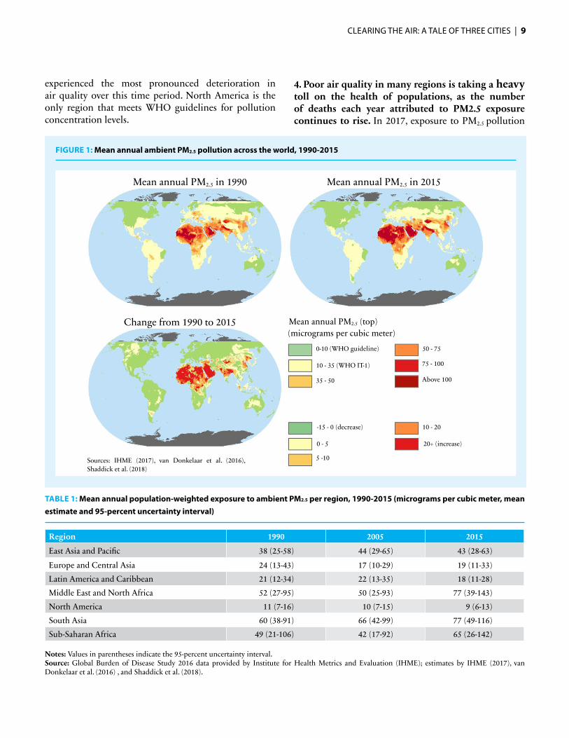
3. Air quality trends have been mixed across the world since the 1990s, with some areas experiencing improvement and others deterioration. The satellite data also indicate the extent to which air pollution has worsened in some regions and improved in others in recent decades. Estimates for average annual PM2.5
concentrations in 1990 and 2015 are illustrated in Figure 1. Table 1 shows average population-weighted exposure by region. Countries in the Middle East and North Africa, Sub-Saharan Africa, and South Asia have
CLEARING THE AIR: A TALE OF THREE CITIES | 9
experienced the most pronounced deterioration in air quality over this time period. North America is the only region that meets WHO guidelines for pollution concentration levels.
4. Poor air quality in many regions is taking a heavy toll on the health of populations, as the number of deaths each year attributed to PM2.5 exposure continues to rise. In 2017, exposure to PM2.5 pollution
FIGURE 1: Mean annual ambient PM2.5 pollution across the world, 1990-2015
Mean annual PM2.5 in 1990 Mean annual PM2.5 in 2015
Mean annual PM2.5 (top)(micrograms per cubic meter)
0-10 (WHO guideline)
10 - 35 (WHO IT-1)
35 - 50
50 - 75
75 - 100
Above 100
10 - 20
20+ (increase)
5 -10
0 - 5
-15 - 0 (decrease)
Sources: IHME (2017), van Donkelaar et al. (2016), Shaddick et al. (2018)
Change from 1990 to 2015
Region 1990 2005 2015East Asia and Pacific 38 (25-58) 44 (29-65) 43 (28-63)Europe and Central Asia 24 (13-43) 17 (10-29) 19 (11-33)Latin America and Caribbean 21 (12-34) 22 (13-35) 18 (11-28)Middle East and North Africa 52 (27-95) 50 (25-93) 77 (39-143)North America 11 (7-16) 10 (7-15) 9 (6-13)South Asia 60 (38-91) 66 (42-99) 77 (49-116)Sub-Saharan Africa 49 (21-106) 42 (17-92) 65 (26-142)
TABLE 1: Mean annual population-weighted exposure to ambient PM2.5 per region, 1990-2015 (micrograms per cubic meter, mean estimate and 95-percent uncertainty interval)
Notes: Values in parentheses indicate the 95-percent uncertainty interval.Source: Global Burden of Disease Study 2016 data provided by Institute for Health Metrics and Evaluation (IHME); estimates by IHME (2017), van Donkelaar et al. (2016) , and Shaddick et al. (2018).
10 | CLEARING THE AIR: A TALE OF THREE CITIES
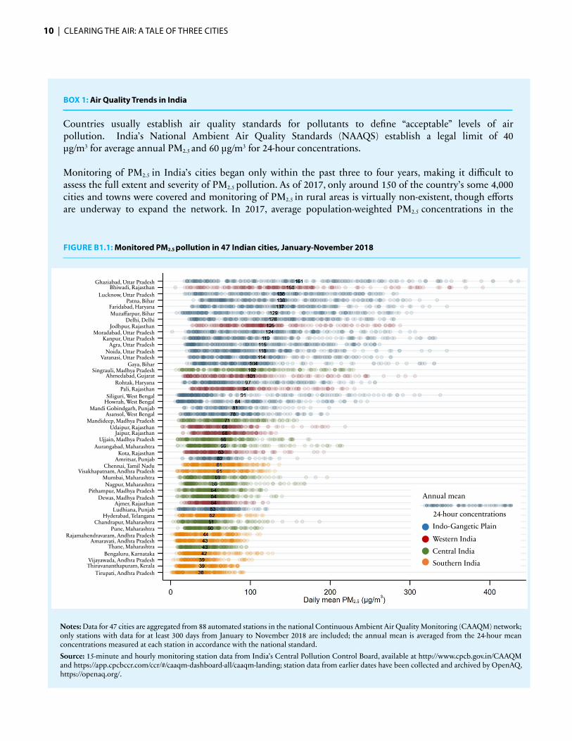
BOX 1: Air Quality Trends in India
Countries usually establish air quality standards for pollutants to define “acceptable” levels of air pollution. India’s National Ambient Air Quality Standards (NAAQS) establish a legal limit of 40 µg/m3 for average annual PM2.5 and 60 µg/m3 for 24-hour concentrations.
Monitoring of PM2.5 in India’s cities began only within the past three to four years, making it difficult to assess the full extent and severity of PM2.5 pollution. As of 2017, only around 150 of the country’s some 4,000 cities and towns were covered and monitoring of PM2.5 in rural areas is virtually non-existent, though efforts are underway to expand the network. In 2017, average population-weighted PM2.5 concentrations in the
Notes: Data for 47 cities are aggregated from 88 automated stations in the national Continuous Ambient Air Quality Monitoring (CAAQM) network; only stations with data for at least 300 days from January to November 2018 are included; the annual mean is averaged from the 24-hour mean concentrations measured at each station in accordance with the national standard.Source: 15-minute and hourly monitoring station data from India’s Central Pollution Control Board, available at http://www.cpcb.gov.in/CAAQM and https://app.cpcbccr.com/ccr/#/caaqm-dashboard-all/caaqm-landing; station data from earlier dates have been collected and archived by OpenAQ, https://openaq.org/.
FIGURE B1.1: Monitored PM2.5 pollution in 47 Indian cities, January-November 2018
Indo-Gangetic Plain
Annual mean
24-hour concentrations
Western IndiaCentral IndiaSouthern India
Ghaziabad, Uttar PradeshBhiwadi, Rajasthan
Lucknow, Uttar PradeshPatna, Bihar
Faridabad, HaryanaMuzaffarpur, Bihar
Delhi, DelhiJodhpur, Rajasthan
Moradabad, Uttar PradeshKanpur, Uttar Pradesh
Agra, Uttar PradeshNoida, Uttar Pradesh
Varanasi, Uttar PradeshGaya, Bihar
Singrauli, Madhya PradeshAhmedabad, Gujarat
Rohtak, HaryanaPali, Rajasthan
Siliguri, West BengalHowrah, West Bengal
Mandi Gobindgarh, PunjabAsansol, West Bengal
Mandideep, Madhya PradeshUdaipur, Rajasthan
Jaipur, RajasthanUjjain, Madhya Pradesh
Aurangabad, MaharashtraKota, Rajasthan
Amritsar, PunjabChennai, Tamil Nadu
Visakhapatnam, Andhra PradeshMumbai, MaharashtraNagpur, Maharashtra
Pithampur, Madhya PradeshDewas, Madhya Pradesh
Ajmer, RajasthanLudhiana, Punjab
Hyderabad, TelanganaChandrapur, Maharashtra
Pune, MaharashtraRajamahendravaram, Andhra Pradesh
Vijayawada, Andhra PradeshThiruvananthapuram, Kerala
Tirupati, Andhra Pradesh
Amaravati, Andhra PradeshThane, Maharashtra
Bengaluru, Karnataka

CLEARING THE AIR: A TALE OF THREE CITIES | 11
10 Data are for 72 monitoring stations covering 40 cities that had data for at least 104 days in 2017, the minimum required by India’s National Ambient Air Quality Standard (NAAQS), out of a total of 288 stations and 137 cities in the network as of the end of 2017. Both manual stations in the National Ambient Air Monitoring Programme (NAMP) and automated stations in the Continuous Ambient Air Quality Monitoring (CAAQM) network are included. The population-weighted average is based on the city population as reported in the 2011 census. NAMP and CAAQM monitoring data are provided by the Central Pollution Control Board at http://cpcb.nic.in/manual-monitoring/ and https://app.cpcbccr.com/ccr/#/caaqm-dashboard-all/caaqm-landing.
monitored cities was 73 µg/m3.10 Only one-third of the cities met the national standard for average annual PM2.5 concentrations; none of the locations with continuous monitoring met the national 24-hour standard; and none of the monitored locations met the WHO guidelines. In 2018, the trends remained largely consistent, with the highest levels of PM2.5 being experienced by cities in the Indo-Gangetic Plain (IGP) (Figure B1.1). Average PM2.5 for cities in the IGP during the first 11 months of 2018 ranged from 53 µg/m3 in Ludhiana, Punjab to 161 µg/m3 in Ghaziabad, Uttar Pradesh. Cities in the IGP and western India frequently experienced days when PM2.5 averaged over 200 µg/m3. Pollution levels in cities in southern India tended to be far lower and without the extreme day-to-day variation seen in the IGP, although still higher than acceptable limits.
Satellite data provide a more complete picture, across the country and over time, as shown in figure B1.2. These data reinforce the spatial disparities in air quality across the regions but also show that air quality has deteriorated across much of the country since the 1990s. According to these estimates,
FIGURE B1.2: Mean annual ambient PM2.5 pollution across the Indo-Gangetic Plain, 1990-2015
1990 - 2015
Sources: IHME (2017), van Donkelaar et al. (2016),Shaddick et al. (2018)
Mean annual PM2.5 in 1990
Mean annual PM2.5 in 2015
Mean annual PM2.5 (top)
Change in mean annual PM2.5 (bottom)
(micrograms per cubic meter)
(micrograms per cubic meter)
0-10 (WHO guideline)
10 - 40 (India NAAOS)
40 - 75
75 - 100
100 - 150
150 - 200
-15 - 0 (decrease)
0 - 5
5 -10
10 - 20
20+ (increase)

12 | CLEARING THE AIR: A TALE OF THREE CITIES
11 The ranges presented here represent 95-percent uncertainty intervals, with a central estimate of 60 µg/m3 for 1990 and 76 µg/m3 for 2015. These estimates of ambient PM2.5 exposure are from the Global Burden of Disease Study 2016 (GBD 2016), an international scientific effort led by the Institute for Health Metrics and Evaluation at the University of Washington, Seattle, United States
12 The ranges represent 95-percent uncertainty intervals. Deaths from exposure to PM2.5 pollution as estimated for the Global Burden of Disease Study 2017 (GBD 2017) and reported here included deaths from acute lower respiratory infections, diabetes, ischemic heart disease, stroke, chronic obstructive pulmonary disease, and lung cancer (Balikrishnan et al. 2018; Stanaway et al. 2018).
resulted in 4.13-5.03 million premature deaths globally, including about 2.50-3.36 million deaths from outdoor ambient PM2.5 and 1.40-1.93 million deaths from PM2.5
in households cooking with solid fuels (Balikrishnan et al. 2018; Stanaway et al. 2018).12 In other words, about 7.4-9.0 percent of attributable deaths globally in 2017 were linked to PM2.5 pollution (Figure 2), more than were caused by HIV/AIDS, tuberculosis, and malaria combined. Furthermore, about half of the deaths attributed to PM2.5
pollution occurred among people younger than 70 years.
5. The health impacts of air pollution also represent a heavy cost to the economy. Public agencies in many countries have taken a variety of approaches to quantifying the economic cost of air pollution and the benefits of policies aimed at reducing pollution. One of the most widely accepted approaches applied by governments is based on individuals’ expressed willingness to pay to reduce their risk of dying.13 Following this approach, the economic cost of fatal illness caused by PM2.5 pollution globally in 2017 was on the order of US$ 2.248 trillion
Notes: “Air pollution (PM2.5)” includes ambient PM2.5 pollution and household PM2.5 pollution from cooking with solid fuels; “WASH” includes unsafe water, sanitation, and handwashing.Source: Institute for Health Metrics and Evaluation, Global Burden of Disease Study 2017 (2018); Stanaway et al. (2018).
FIGURE 2: Leading fatal health risks globally, 2017
Share of all-cause mortality globally in 2017(%)
Metabolic risks 31.4Dietary risks 19.5
Tobacco 14.5Air pollution (PM2.5) 8.2Child and maternal
malnutrition 5.7WASH 2.9
Low physical activity 2.3
0 5 10 15 20 25 30 35
the average level of outdoor or “ambient” PM2.5 pollution to which people are exposed each year rose from 39-89 µg/m3 in 1990 to 49-112 µg/m3 in 2015 (IHME 2017; van Donkelaar et al. 2016; Gakidou et al. 2017; Shaddick et al. 2018).11 Anywhere from 732 million to 1.270 billion people in India (56-97 percent of the country ’s population) were exposed to ambient PM2.5 in 2015 above the NAAQS, up from 339-829 million in 1990. Some regions have seen improvements in air quality (areas in green in the bottom panel of Figure B1.2), though concentrations remain high and above healthy levels even in these areas. Finally, poor air quality is not only an urban issue. As Figure B1.2 shows, air pollution particularly in the IGP and a few other regions is widespread and affects rural communities as well as people in cities.

CLEARING THE AIR: A TALE OF THREE CITIES | 13
13 Economists use a variety of methods to elicit people’s willingness to pay (WTP). One method is through so-called stated preference surveys. When people who are surveyed tell economists how much they are willing to pay to reduce their fatality risk, they are thinking about much more than their paychecks. Losses may also reflect the loss of enjoyment that people get from intangibles such as being alive or spending time with loved ones. Another method is by looking at the differences in wages for more or less risky jobs. The estimates of the costs of pollution presented here are based primarily on findings from stated preference surveys. For a discussion of why, please refer to Narain and Sall (2016).
14 Monetary losses are reported in terms of US dollars calculated at constant year 2011 prices on a purchasing power parity (PPP) basis. Global welfare losses here represent the sum of losses as calculated for 168 countries. See World Bank-IHME (2016) for a description of how the uncertainty interval is calculated based on varying key assumptions such as WTP for reduced fatality risk using a database of WTP estimates from stated preference studies around the world. The central estimate represents the median estimate from 5,000 random draws.
15 Global estimates presented here are for 164 countries. Fewer countries have the necessary data to calculate forgone labor output than welfare losses. As above, see World Bank-IHME (2016) for a description of how the uncertainty interval is constructed.
to US$ 13.692 trillion (95-percent uncertainty interval), with a central estimate of US$ 4.334 trillion.14 The wide range accounts for uncertainty owing to the health impacts as well as people’s willingness to pay. In other words, even under the most conservative scenario, the annual economic cost of PM2.5 pollution is equivalent in magnitude to at least 1.9 percent of the world GDP. (Costs are expressed as an equivalent percent of GDP just to provide a convenient sense of scale, not to suggest they are a direct loss of GDP. GDP is a measure of output, not economic wellbeing.) As an alternative, other governments have also measured the loss of human capital due to fatal illness. Under this approach, losses are estimated in terms of the expected labor income that people would have earned over their lifetimes had they not died prematurely. The estimated loss of income is typically much smaller than the total economic cost of fatal illness as estimated based on individuals’ willingness to pay, reflecting how people value more than just their paychecks. Alternatively, if losses are calculated only on the basis of forgone lifetime labor earnings, the expected
loss of income loss due to fatal illness from PM2.5 pollution in 2017 would be in the range of US$ 131-317 billion globally, with a central estimate of US$ 200 billion, equal in magnitude to 0.1-0.3 percent of GDP.15
6. Apart from the cost of fatal illness, air pollution impacts a country’s economy in other ways too. Ground-level ozone (O3) pollution, for example, which forms when volatile organic compounds (VOCs) react with NOx, is toxic to plants and has been shown to reduce crop yields. One study found that ozone and black carbon (emitted mostly from household cookstoves) cut yields of wheat and rice by about 33 percent and 22 percent, respectively, in India’s largest producing states in 2010. Lower yields translated into a loss of 24 million tons of harvested wheat alone, worth about US$ 5 billion (Burney and Ramanathan, 2015). Elsewhere, research from China shows that air pollution is also making skilled workers in urban areas less productive (Chang et al. 2016), suggesting that worsening air quality may be dulling the competitive edge of cities too.

14 | CLEARING THE AIR: A TALE OF THREE CITIES
What is the relationship between air quality and economic growth?

What is the relationship between air quality and economic growth?
1. Low income and lower-middle income countries (LICs and LMCs) have experienced deteriorating air quality since 1990, though not upper-middle and high-income countries (see Table 2). Between 1990 and 2015, mean annual PM2.5 in LICs increased from 44 µg/m3 to 56 µg/m3, while mean annual PM2.5 in the LMCs (excluding India) rose from 45 µg/m3 to 59 µg/m3. In India, during this time period, mean annual PM2.5 also increased, from an average of 60 µg/m3 in 1990 to 76 µg/m3 in 2015. At the same time, ambient PM2.5 stabilized in some upper-middle-income – China -- and improved in others – Mexico, for example -- and in high-income countries. These trends imply that the disparity in air quality between poorer and richer countries has grown over time, as further illustrated in Figure 3. In the figure, blue dots represent mean annual PM2.5 concentrations at different levels of per capita income in 2015, and orange dots the same in 1990. A steeper trend line in 2015 illustrates the growing disparity.
Income Group or Country 1990 2005 2015Low income 44 (15-106) 40 (14-96) 56 (19-137)India (lower middle income) 60 (39-89) 66 (42-98) 76 (49-112)Other lower middle income 45 (24-79) 44 (24-76) 59 (31-104)China (upper middle income) 48 (31-72) 57 (38-83) 56 (38-82)Mexico (upper middle income) 25 (15-37) 26 (16-39) 19 (12-28)Other upper middle income 26 (15-45) 23 (13-39) 25 (14-44)High income 18 (11-26) 16 (10-23) 19 (12-29)
Notes: Values in parentheses indicate the 95-percent uncertainty interval; data for China, India, and Mexico are highlighted in grey; income group classifications are as of the 2015 calendar year.Source: Global Burden of Disease Study 2016 data provided by Institute for Health Metrics and Evaluation (IHME); estimates by IHME (2017), van Donkelaar et al. (2016), and Shaddick et al. (2018).
TABLE 2: Mean annual population-weighted exposure to ambient PM2.5 per income group and for China, India, and Mexico, 1990-2015 (micrograms per cubic meter, mean estimate and 95-percent uncertainty interval)
Notes: Mean annual PM2.5 is population-weighted mean exposure; PM2.5 and GNI per capita are rescaled logarithmically.Source: Global Burden of Disease Study 2016 data provided by Institute for Health Metrics and Evaluation (IHME); estimates by IHME (2017), van Donkelaar et al. (2016), and Shaddick et al. (2018); GNI per capita data from World Bank, World Development Indicators database.
Mea
n an
nual
PM
2.5
GNI per capita (constant 2010 US$)
160
80
40
20
10
5250 1,000 4,000 16,000 64,000
199020151990 trend2015 trend
FIGURE 3: Mean annual ambient PM2.5 pollution versus GNI per capita, 1990 and 2015

16 | CLEARING THE AIR: A TALE OF THREE CITIES
2. These trends would seem to reinforce that the experience of any country is part of a larger trend consistent with the so-called “Environmental Kuznets Curve”. Named after Simon Kuznets, who theorized that income inequality initially worsens and then improves at higher levels of income as a country develops (Kuznets, 1955), the notion that pollution and income also form an inverted U-shaped curve was first popularized in the early 1990s and is referred to as the Environmental Kuznets Curve (EKC).16 The possibility that a country’s development path follows an EKC, raises the question whether poor air quality is a reflection of a country’s low level of development. Will countries simply grow their way out of pollution?
3. Large middle-income countries appear to be on very different growth paths when assessed by the level of pollution intensity. Figure 4 illustrates the relationship between mean annual PM2.5 exposure and the level of income, as measured by GDP per capita, for large middle-income countries from 1990 to 2015. A few countries – China and Mexico among them – appear to follow the inverted U-shaped curve, where pollution first increases as the country grows. These countries appear to have reached a turning point, though at different levels of income per capita, after which pollution started to fall. Number of other countries are yet to reach a turning point and mean annual PM2.5 is increasing in these countries along with income. Among this group of countries, countries in South Asia – India, Nepal, and Pakistan – stand out and appear to have a more pollution-intensive growth path than countries of similar income levels, where pollution intensity is measured by the steepness of the curve. Econometric analysis further reveals that income elasticity of ambient PM2.5 is systematically higher in the South Asia region than for other regions, even after accounting for differences in economic structure, demographics, energy supply, and natural characteristics such as topography and climate (see Annex).
4. Trends at the state-level within India also suggest that economic growth has been much more pollution-intensive in some parts of the country than in others. Figure 5 compares GDP per capita in purchasing power parity (PPP) terms with mean annual exposure to PM2.5 in the various states and regions of India. Trends for China and Mexico are shown for comparison. As the figure reveals, India’s pollution-intensive growth pattern is driven primarily by trends in states of the IGP, including Bihar, Delhi, Haryana, Jharkhand, Punjab, Uttar Pradesh, and West Bengal. These seven states had the highest elasticities of PM2.5 with respect to income, although at markedly different levels of per capita income: Bihar and Jharkhand had the lowest levels of GDP per capita in the country, while Delhi and Haryana had the highest. Other than states in the IGP, states in Central India, and Western states appear to be on more pollution-intensive development paths. Box 2 explores the reasons underlying these somewhat paradoxical trends.
16 One of the first empirical studies to suggest the existence of an EKC was a 1991 paper by Grossman and Krueger. Responding to concerns that environmental quality in Mexico might suffer if its economy was opened to polluting industries under the North American Free Trade Agreement, Grossman and Krueger (1991) tested how air quality in a cross-section of cities in more than 40 countries varied across different levels of GDP per capita and trade openness (exports as a share of GDP). They found that average concentrations of SO2 and smoke tended to increase with GDP per capita in the lowest-income countries but then fell as GDP continued to increase beyond a certain level.
FIGURE 4: GDP per capita versus mean annual ambient PM2.5 in select large middle-income countries, 1990-2015
Source: Global Burden of Disease Study 2016 data provided by Institute for Health Metrics and Evaluation (IHME); estimates by IHME (2017), van Donkelaar et al. (2016), and Shaddick et al. (2018); GDP per capita data from World Bank, World Development Indicators database.
Pakistan
Myanmar Iran, Islamic Rep.
Turkey
KazakhstanMexico
Brazil
Thailand
Sri LankaSouth Africa
0 5,000
GDP per capita, 1990-2015 (year 2011 US$, PPP)
10,000 15,000 20,000 25,000
UkraineVietnam
China
India
Mea
n an
nual
PM
2.5,1
990-
2015
(μg/
m3 )
80
70
60
50
40
30
20
10
0
Nepal

CLEARING THE AIR: A TALE OF THREE CITIES | 17
a. Indo-Gangetic Plain (plus China and Mexico)
160
140
120
100
80
60
40
20
0 0 2,000 4,000 6,000 8,000 10,000 12,000 14,000 16,000GDP per capita (2011 US$, PPP)
Mea
n an
nual
PM
2.5 (μ
g/m
3 )
Mexico
China
JharkhandWest Bengal Punjab
HaryanaUttar Pradesh
Bihar
Delhi
c. Southern States160
140
120
100
80
60
40
20
0
Mea
n an
nual
PM
2.5 (μ
g/m
3 )
Mexico
China
Karnataka
Andhra PradeshTamil Nadu
Kerala
Telangana
0 2,000 4,000 6,000 8,000GDP per capita (2011 US$, PPP)
10,000 12,000 14,000 16,000
e. Western Himalayan States
160
140
120
100
80
60
40
20
0
Mexico
0 2,000 4,000 6,000 8,000GDP per capita (2011 US$, PPP)
10,000 12,000 14,000 16,000
Mea
n an
nual
PM
2.5 (μ
g/m
3 )
ChinaJammu and Kashmir
Himachal Pradesh
Uttarakhand
b. Central States
160
140
120
100
80
60
40
20
0 0 2,000 4,000 6,000 8,000 10,000 12,000 14,000 16,000GDP per capita (2011 US$, PPP)
Mea
n an
nual
PM
2.5 (μ
g/m
3 )
Chhattisgarh
Madhya PradeshOdisha
MaharashtraChina
Mexico
d. Northeastern States160
140
120
100
80
60
40
20
0
Mea
n an
nual
PM
2.5 (μ
g/m
3 )
0 2,000 4,000 6,000 8,000GDP per capita (2011 US$, PPP)
10,000 12,000 14,000 16,000
Mexico
China
Sikkim
Mizoram
Assam Tripura
Meghalaya
Arunachal PradeshManipur
f. Western States
Mexico
China
150
125
100
75
50
25
0
Mea
n an
nual
PM
2.5 (μ
g/m
3 )
RajasthanGujarat
Assam
0 2,000 4,000 6,000 8,000GDP per capita (2011 US$, PPP)
10,000 12,000 14,000 16,000
FIGURE 5: Mean annual PM2.5 pollution and GDP per capita in various regions of India, 1990-2015
Notes: “PPP” = purchasing power parity.Sources: Ambient PM2.5 exposure data from Global Burden of Disease Study 2016, as provided by IHME; estimates by IHME (2017), van Donkelaar et al. (2016) , and Shaddick et al. (2018); gridded GDP data from Kummu et al. (2018).

18 | CLEARING THE AIR: A TALE OF THREE CITIES
BOX 2: Explaining two paradoxes about pollution intensity of India’s growth path
State-level trends of air pollution and economic growth shown in Figure 5 reveal two seeming paradoxes about India’s growth path. First, how can some states with the lowest GDP per capita and slowest rates of economic growth also suffer from the worst air pollution? Such high levels of air pollution are commonly associated with the processes of industrialization and urbanization, which tend to occur at relatively higher levels of income per capita than the current levels in the poorest states of the IGP. Second, how can states such as Delhi, Haryana, and Punjab have high levels of pollution despite being relatively rich? As shown in Figure 4, countries at income levels comparable to these three states were able to improve their air quality while continuing to grow. Why have these three states not been able to do the same?
Recent studies examining how emissions from different sectors have contributed to overall ambient concentrations of pollution in the air that people breathe across Indian states reinforce the cross-sector and cross-border nature of pollution in India, offering an explanation for the paradoxes. Analysis by the Council on Energy, Environment and Water (CEEW) and International Institute for Applied Systems Analysis (IIASA) sheds light on the contribution of different sectors and different regions to poor air quality in a particular region. Figure B2.1 shows that residential emissions from households using solid fuels for heating and cooking, emission from industry, power plants, agriculture, and transport, and natural dust all contribute to poor air quality, though to differing levels in different states. It also points to the significant contribution of secondary PM2.5 formed by reactions involving other pollutants. Because PM2.5 can remain suspended in the atmosphere for
Source: CEEW-IIASA (2018).
PM2.
5 (μ
g/m
3 )
120
100
80
60
40
20
0
Him
acha
l Pra
desh
Jam
mu,
Kas
hmir
Mad
hya
Prad
esh
Goa
Raj
asth
an
Chh
attis
garh
Karn
atak
a
Har
yana
Guj
arat
Odi
sha
And
hra
Prad
esh*
Punj
ab
Utta
rakh
and
Mah
aras
htra
Biha
r
Jhar
khan
d
Nor
th E
ast
Utta
r Pra
desh
Del
hi
Wes
t Ben
gal
Ass
am
Kera
la
Tam
il N
adu
NAAQS
WHO guideline
Natural sources Secondary PM2.5* Coal thermal power plants Other high stacks
Households Transport Waste Agriculture
FIGURE B2.1: State-wise origin of mean annual population-weighted ambient PM2.5 by sector, 2015

CLEARING THE AIR: A TALE OF THREE CITIES | 19
long periods of time and travel hundreds or thousands of kilometers, PM2.5 emissions can cross state boundaries. Figure B2.2 captures this characteristic feature of PM2.5 concentrations finding that states and Union Territories (UTs) with the greatest amount of ambient PM2.5 originating from other states and regions in India include Bihar, Delhi, Haryana, Jharkhand, and Odisha. These results suggest that individual states acting in isolation are unlikely to solve their air quality problems on their own.
The high levels of pollution at relatively low levels of development in four IGP states and the high level of pollution in the three IGP states with the highest GDP per capita can be explained by a combination of factors that follow from the contribution of the different sources to air pollution and regional nature of the challenge.
Agricultural intensification, high population density, a high reliance on residential biomass, and regional sources of PM2.5 from other states and areas help explain the high levels of pollution in the IGP at relatively low levels of economic development. Low levels of development are characterized by a high share of agriculture in the economy and certain consumption patterns, such as a high degree of dependence on biomass for cooking and heating. In fact, most of India’s IGP is covered by cropland (about 85 percent of the land area), scattered with a few large (7) and medium-sized (22) cities and many smaller cities (37) and towns (648). The agriculture sector is an important contributor to the economy as well as PM2.5 pollution, with intensive farming, high fertilizer use, and the seasonal burning of crop residues. Consequently, Chakraborty and Gupta (2010) found
FIGURE B2.2: Contribution of local, regional, and transboundary sources of ambient PM2.5 exposure in Indian states, 2015 (micrograms per cubic meter)
Source: CEEW-IIASA (2018).
Natural sources
Mad
hya
Prad
esh
120
100
80
60
40
PM2.
5 (μg
/m3 )
20
0
Goa
Raj
asth
an
Chh
attis
garh
Karn
atak
a
Har
yana
Guj
arat
Odi
sha
And
hra
Prad
esh*
Punj
ab
Utta
rakh
and
Mah
aras
htra
Biha
r
Jhar
khan
d
Nor
th E
ast
Him
acha
l Pra
desh
Utta
r Pra
desh
Del
hi
Wes
t Ben
gal
Ass
am
Kera
la
Tam
il N
adu
Jam
mu
and
Kash
mir
NAAQS
WHO guideline
Outside India Other India Neighboring States This States
20 | CLEARING THE AIR: A TALE OF THREE CITIES
that secondary sources (with NH3 from agriculture reacting with NOx and SO2) contributed about 40 percent of PM2.5 concentrations in the city of Kanpur in Uttar Pradesh. High population density in rural areas compounds the problem, with households continuing to depend primarily on biomass for cooking and heating. Apart from Tamil Nadu and Kerala, the states in the IGP have the highest population density of any in the country. High population density and low levels of development also make small township-based industries an important source. Finally, due to features of the IGP’s geography and climate, the dispersion of pollution is weak, particularly in the winter months, and pollution from upwind areas is funneled into the region, adding to the challenge.
The same factors, combined with greater emissions from motor vehicles, further help to explain why India’s states with the highest levels of GDP per capita—Delhi, Haryana, and Punjab—also experience some of the worst pollution. Studies in the Delhi National Capital Region (NCR) have found that vehicular emissions contribute about 23-25 percent of ambient PM2.5 in the winter and about 19 percent of mean annual ambient PM2.5. Also, although cooking and heating with liquified petroleum gas (LPG), electricity, and natural gas is more common in urban districts of the NCR and surrounding areas, the three states also continue to have a high density of households reliant on solid fuels. Furthermore, as in the other states in the IGP, agriculture continues to be an important economic sector for Punjab and Haryana, with farming characterized by greater intensification, higher fertilizer use, and the seasonal burning of crop residues. Regional sources of air pollution also contribute a large share of overall ambient PM2.5 concentrations, with as much as 60 percent of Delhi’s pollution coming from neighboring states (Amman et al. 2016).
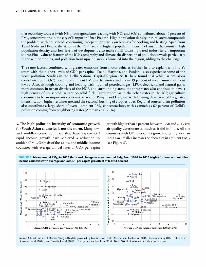
FIGURE 6: Mean annual PM2.5 in 2015 (left) and change in mean annual PM2.5 from 1990 to 2015 (right) for low- and middle-income countries with average annual GDP per capita growth of at least 3 percent
Source: Global Burden of Disease Study 2016 data provided by Institute for Health Metrics and Evaluation (IHME); estimates by IHME (2017), van Donkelaar et al. (2016), and Shaddick et al. (2018); GDP per capita data from World Bank, World Development Indicators database.
MyanmarChina
Bosnia and Herzegovina Azerbaijan
ArmeniaMozambique
AlbaniaSri Lanka
Lao PDRAngola
MongoliaTurkmenistan
UzbekistanEthopia
Rwanda
India
Cambodia
IraqSudan
Uganda
ChadBangladesh
Nigeria
140
120
100
80
60
40
20
02 3
Average GDP per capita growth rate, 1990-2015 (%)
Mea
n an
nual
PM
2.5 in
201
5 (μ
g/m
3 )
4 5 6 7 8 9 10
Vietnam
MyanmarChina
Bosnia and Herzegovina
AzerbaijanArmenia
Sri Lanka
Georgia Lao PDR
Belarus
Albania
Mongolia
Bulgaria
RomaniaMoldova
UzbekistanThailand
Malasia
Ethopia
Serbia
India
Cambodia
IraqSudan
Uganda
Chad
BangladeshNigeria
40
30
20
10
0
-10
-20
-302 3
Average GDP per capita growth rate, 1990-2015 (%)
Cha
nge
in m
ean
annu
al P
M2.
5 in
199
0-20
15 (μ
g/m
3 )
4 5 6 7 8 9 10
Vietnam
5. The high pollution intensity of economic growth for South Asian countries is not the norm. Many low- and middle-income countries that have experienced rapid income growth have achieved a reduction in ambient PM2.5. Only six of the 42 low and middle-income countries with average annual rates of GDP per capita
growth higher than 3 percent between 1990 and 2015 saw air quality deteriorate as much as it did in India. All the countries with GDP per capita growth rates higher than India saw smaller increases or decreases in ambient PM2.5 (see Figure 6).

CLEARING THE AIR: A TALE OF THREE CITIES | 21
6. These trends reinforce the role of policies and programs in affecting the shape of the relationship between economic growth and pollution, suggesting that countries cannot simply grow their way out of pollution. Although the existence of the EKC continues to be debated in the academic literature (see Stern 2015 for a recent review), critics have rightly questioned its shaky
17 Indeed, this point was raised by one of the earliest EKC studies, published in 1992 by World Bank economists Nemat Shafik and Sushenjit Bandyopadhyay, and is worth revisiting. Shafik and Bandyopadhyay tracked the relationship of income, investment, trade, debt and other macroeconomic characteristics with a variety of indicators for environmental quality, including mean annual concentrations of TSP in cities. Looking at trends in urban air quality across countries from the 1970s to the 1980s, they found evidence of an inverted U-shaped relationship of TSP with income—like that observed for SO2 and smoke by Grossman and Krueger (1991). They conclude: “The evidence suggests that it is possible to ‘grow out of’ some environmental problems. But there is nothing automatic about this—policies and investments must be made to reduce degradation” (Shafik and Bandyopadhyay 1992: 23). As they note, not all indicators of environmental quality improved at higher income levels: carbon emissions and municipal waste per capita, for example, increased exponentially.
foundation. Policy decisions, investments, technologies, and external shocks can bend, flatten, or shift the curve (Payanotou 1997; Unruh and Moomaw 1998; Dasgupta et al. 2002), meaning that countries cannot simply rely on economic growth to produce a cleaner environment in the end.17

22 | CLEARING THE AIR: A TALE OF THREE CITIES
Tackling air pollution: Lessons from Mexico City, Beijing, and Delhi

1. Role of policies, technologies, and investments Come to light when one looks at the experience of many countries, and urban agglomerations within them, that have successfully tackled the air pollution challenge. Three cities -- Mexico City, Beijing, and Delhi – offer lessons for other cities as they take on the fight to reduce air pollution.
3A. AIR QUALITY MANAGEMENT IN MEXICO CITY
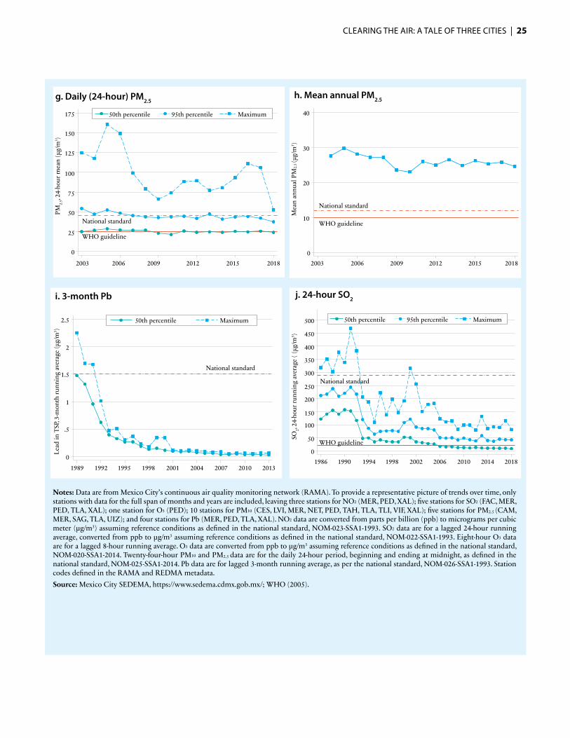
2. Mexico City suffered from hazardous air pollution in the 1980s and 1990s, as a result of rapid population growth, industrialization, and motorization. In 1992, a comparison of key pollutants – lead (Pb), sulfur dioxide (SO2) and total suspended particles (TSP) -- across several mega cities in Mexico led the World Health Organization and the United Nations Environment Program to conclude that Mexico City was the most polluted megalopolis on the planet (WHO-UNEP 1992). Monitoring data for these pollutants and nitrogen oxide (NOx) and ozone (O3) collected in the city beginning in 1986 showed that pollution frequently exceeded national standards and the WHO air quality guidelines (see Figure 7).
3. Facing a public health crisis, the Government of Mexico launched the first multi-year air quality management strategy in 1990. At this time Mexico City was known as the Federal District and was administered by the Chief of the Federal District, as part of the Federal Administration and reporting directly to the President. In response to the President’s call to act immediately to abate air pollution, an inter-agency working group was established that included representatives from the Ministries of Urban Development and Environment, Finance, Planning and Budget, Commerce and Industrial Promotion, Health, Energy, Mines and State-Owned Industries, Agriculture and Hydraulic Resources, and Transport and Communications, as well as representatives
from the Governments of the Federal District and the State of Mexico, municipal governments in the greater metropolitan area, the Federal Electricity Commission, the Mexican Institute of Petroleum, and the Mexican state-owned petroleum company -- Pemex. The working group developed the Integrated Program against Atmospheric Pollution in the Mexico City Metropolitan Area (PICCA) for 1990-1994 (GoM 1990), the first air quality management strategy.
4. A number of measures were implemented as part of the PICCA to reduce air pollution. Under the PICCA, pollution abatement measures were introduced in the greater metropolitan area, which then encompassed Mexico City and 17 municipalities from the State of Mexico. The biggest achievements were: improving fuel quality (phasing out of lead in gasoline, introduction of oxygenated gasoline, introduction of diesel with a maximum sulfur content of 500 PPM, and substitution of heavy fuel oil with light fuel oil in 1991 and gasoil in 1995), installation of pollution control technologies in vehicles (three way catalytic converters, evaporative emission controls, and electronic fuel injection and ignition accessories), and the establishment of stricter vehicular pollution norms (GoM, n.d.). As a result, Pb, carbon monoxide (CO), PM10, and SO2 emissions fell significantly, and O3 emission levels stabilized (GoM 1996). Pollution declined dramatically in just a few years (see Figure 7).
5. Building on lessons from the implementation of PICCA, additional programs were introduced to control air pollution, starting in the mid-90s. PICCA was followed by the Program to Improve Air Quality (PROAIRE) 1995-2000, that included for the first time in Mexico quantitative air quality improvement goals. The PROAIRE’s main goal was to reduce peak and average concentrations of ozone, which had not been reduced significantly under PICCA. Though PROAIRE succeeded in reducing O3 levels significantly, concentrations of O3 remained above the legal standard for more than 80
Tackling air pollution: Lessons from Mexico City, Beijing, and Delhi

24 | CLEARING THE AIR: A TALE OF THREE CITIES
FIGURE 7: Monitored concentrations of pollutants in Mexico City compared to national standards and WHO guidelines, January 1986 to September 2018
a. Hourly NO2
1986
700650600550500450400350300250200150100500
1990 1994 1998 2002 2006 2010 2014 2018
Hou
rly N
O2 (
μg/m
3 )
WHO guideline
National standard
50th percentile 95th percentile Maximum
b. Mean Annual NO2
Mea
n an
nual
NO
2 (μg
/m3 )
WHO guideline
100
90
80
70
60
50
40
30
20
10
01986 1990 1994 1998 2002 2006 2010 2014 2018
c. Hourly O3
Hou
rly o
zone
(μg/
m3 )
900
800
700
600
500
400
300
200
100
0
National standard
50th percentile 95th percentile Maximum
1986 1990 1994 1998 2002 2006 2010 2014 2018
d. 8-hour O3
Ozo
ne, 8
-hou
r run
ning
ave
rage
(μg/
m3 )
National standard
WHO guideline
600550
500
450
400
350
300
250
200
150
100
50
0
50th percentile 95th percentile Maximum
1986 1990 1994 1998 2002 2006 2010 2014 2018
e. Daily (24-hour) PM10
National standard
WHO guideline
1995 2000 2005 2010 2015
450
400
350
300
250
200
150
100
50
0
PM10
, 24-
hour
mea
n (μ
g/m
3 )
50th percentile 95th percentile Maximum
f. Mean annual PM10
80
70
60
50
40
30
20
10
01995 2000 2005 2010 2015
Mea
n an
nual
PM
10 (μ
g/m
3 )
National standard
WHO guideline
CLEARING THE AIR: A TALE OF THREE CITIES | 25
g. Daily (24-hour) PM2.5h. Mean annual PM2.5
i. 3-month Pb
2003 2006 2009 2012 2015 2018
175
150
125
100
75
50
25
0
PM2.
5, 24
-hou
r mea
n (μ
g/m
3 )
National standard
WHO guideline
50th percentile 95th percentile Maximum
2003 2006 2009 2012 2015 2018
40
30
20
10
0
Mea
n an
nual
PM
2.5 (μ
g/m
3 )
National standard
WHO guideline
1989 1992 1995 1998 2001 2004 2007 2010 2013
Lead
in T
SP, 3
-mon
th ru
nnin
g av
erag
e (μ
g/m
3 )
National standard
50th percentile Maximum2.5
2
1.5
1
.5
0
j. 24-hour SO2
1986 1990 1994 1998 2002 2006 2010 2014 2018
500
450
400
350
300
250
200
150
100
50
0
SO2,
24-h
our r
unni
ng a
vera
ge (
(μg/
m3 )
National standard
WHO guideline
50th percentile 95th percentile Maximum
Notes: Data are from Mexico City’s continuous air quality monitoring network (RAMA). To provide a representative picture of trends over time, only stations with data for the full span of months and years are included, leaving three stations for NO2 (MER, PED, XAL); five stations for SO2 (FAC, MER, PED, TLA, XAL); one station for O3 (PED); 10 stations for PM10 (CES, LVI, MER, NET, PED, TAH, TLA, TLI, VIF, XAL); five stations for PM2.5 (CAM, MER, SAG, TLA, UIZ); and four stations for Pb (MER, PED, TLA, XAL). NO2 data are converted from parts per billion (ppb) to micrograms per cubic meter (µg/m3) assuming reference conditions as defined in the national standard, NOM-023-SSA1-1993. SO2 data are for a lagged 24-hour running average, converted from ppb to µg/m3 assuming reference conditions as defined in the national standard, NOM-022-SSA1-1993. Eight-hour O3 data are for a lagged 8-hour running average. O3 data are converted from ppb to µg/m3 assuming reference conditions as defined in the national standard, NOM-020-SSA1-2014. Twenty-four-hour PM10 and PM2.5 data are for the daily 24-hour period, beginning and ending at midnight, as defined in the national standard, NOM-025-SSA1-2014. Pb data are for lagged 3-month running average, as per the national standard, NOM-026-SSA1-1993. Station codes defined in the RAMA and REDMA metadata.Source: Mexico City SEDEMA, https://www.sedema.cdmx.gob.mx/; WHO (2005).

26 | CLEARING THE AIR: A TALE OF THREE CITIES
percent of the days in 2000. The next phase of PROAIRE (2002-2010) incorporated new scientific information and adopted goals to reduce the number of days in which the concentrations of O3, PM10, SO2, and CO exceeded respective air quality standards. A national standard for PM2.5 concentrations was also introduced for the first time in 2004. The interventions implemented under the second PROAIRE helped to reduce the emissions of all measured pollutants but annual concentrations of PM10 and PM2.5 and daily concentrations for O3 continued to exceed the legal standards. PROAIRE 2011-2020 built on previous experience, incorporated the latest scientific findings, and proposed managing the Mexico City Metropolitan Area (MCMA) as an ecosystem (MESM-MEFD-MENR-MH 2011). Finally, in 2017, Secretariat of Environment and Natural Resources (Secretaria del Medio Ambiente y Recursis Naturales, “SEMARNAT”) published the “Federal Program to Improve Air Quality in the Megalopolis: PROAIRE of the Megalopolis 2017-2030.” (MENR 2017).
6. Coordination between the federal and local governments has been key to air quality management in the Mexico City Metropolitan Area. In 1992, the Metropolitan Environmental Commission (CAM) was created by Presidential Decree to improve coordination between federal and local government agencies in the airshed.18 The CAM brought together federal authorities from the ministries of environment, health, and transport and local authorities from the Federal District (now Mexico City) and the State of Mexico. The Federal Government also established a trust fund that would serve as CAM’s financial mechanism and that was funded by a gasoline charge that was in place between 1995 and 1997 (NIGSI 2005). In its early years, the CAM struggled to fulfill its role as the coordinating body for air quality management due to frequent personnel changes, lack of an independent budget, lack of enforcement powers, and an unclear organizational structure (Molina and Molina 2006). However, CAM’s gradual strengthening allowed it to play an instrumental role in the development and implementation of PICCA and air quality programs (PROAIRE) for 1995-2000, 2002-2010, and 2011-2020. The CAM evolved into the Megalopolis Environmental
Commission (la Comisión Ambiental de la Megalópolis, “CAMe”) in 2013, to cover a greater geographic area, recognizing that the metropolitan area had grown and that the sources of and responses to pollution required a geographical coverage that was wider than CAM’s. CAMe’s geographical coverage included Mexico City and a total of 224 municipalities in the surrounding states of Hidalgo, Mexico, Morelos, Puebla, and Tlaxcala. In addition, CAMe had a more comprehensive governance structure that included a high level government body (with Mexico’s Minister of Environment and Natural Resources, the five state governors, and the Chief of Mexico City’s Government), an Executive Commissioner, and a Scientific Advisory Committee.19 States that were part of CAMe agreed in 2014 to transfer to the commission MX$ 5.00 for each vehicle inspection conducted within their jurisdiction to complement the trust fund created in 1992 to finance new environmental projects.
18 The commission was established by a Presidential Decree published on January 8, 1992 and its original name was the Commission for the Prevention and Control of Atmospheric Pollution in the Metropolitan Area of the Valley of Mexico. The Governments of the Federal District Department, the State of Mexico and the State of Hidalgo signed an agreement on September 13, 1996 to increase the commission’s geographic coverage to the entire Federal District, 59 municipalities in the State of Mexico and 29 municipalities in the State of Hidalgo. The agreement also changed the commission’s name to Metropolitan Environmental Commission (Comisión Ambiental Metropolitana-CAM).
19 Agreement published in the Diario Oficial de la Federación, October 3, 2013
Year PM10 PM2.5 SO2 NOx VOC1998 36% N/A 21% 81% N/A2004 23% 57% 45% 82% 35%2008 16% 52% 49% 82% 31%2016 53% 56% 28% 86% 17%
Source: Emissions Inventory of the Mexico City Metropolitan Area 1998, 2004, 2008, and 2016.
TABLE 3: Primary Emissions from Mobile Sources in the Mexico City Metropolitan Area (% of total emissions, selected years)
7. Reducing pollution from vehicles has remained a top priority of the Mexico City Metropolitan Area (MCMA) pollution management strategy. Emissions inventories published since 1998 showed that mobile sources are a key source of primary particle emissions in the MCMA and precursors to secondary pollutants, particularly PM2.5 and oxidants like ozone (see Table 3). Policies aimed at reducing harmful emissions from vehicles in the MCMA have combined gradually tighter standards, improved inspection and maintenance, and monetary incentives. Air quality management plans for

CLEARING THE AIR: A TALE OF THREE CITIES | 27
20 Norma Oficial Mexicana NOM-086-SEMARNAT-SENER-SCFI-2005, Especificaciones de los Combustibles Fósiles para la Protección Ambiental.
2002- 2010 and 2011-2020 (“PROAIRE 2002-2010” and “PROAIRE 2011-2020”) include vehicular emission reduction policies such as:
< Progressively tighter fuel quality standards: State and local authorities have coordinated with the Federal Government and PEMEX through the CAM (and later CAMe) to advocate for more stringent fuel standards An official norm published in January 2006 (NOM-086-SEMARNAT-SENER-SCFI-2005) restricted the sulfur content in premium gasoline to a maximum of 80 parts per million (PPM) by October 2006 and required a similar sulfur content for magna gasoline sold in the MCMA by October 2008. The same norm required that only diesel with a maximum sulfur content of 15 ppm be sold in the MCMA by January 2009.20 In the rest of the country, the use of ultra-low sulfur diesel was required starting in December 2018, bringing Mexico’s fuel quality in line with the highest European and US standards (NIECC 2019).
< Vehicle emissions standards: Vehicle emissions standards have been progressively tightened in step with better fuel quality. Mexico City has anticipated tightening emissions standards and forged ahead of the national timetable by adopting standards equivalent to the strictest European and US standards (Euro VI or US EPA 2010) as part of its voluntary inspection and maintenance program (see Table 4). Nationwide implementation of
Euro VI/US EPA 2010 standards is not scheduled until 2021.
< Subsidies and low-cost loans for the replacement and upgrading of taxis and buses: By the early-2000s, there were about 110,000 taxis on the streets of the greater metropolitan area and most of these were at least nine years old. Due to their age and the long distances traveled each day, taxis contributed an oversized share of NOx, CO, VOC, and PM emissions. To confront this problem, during the PROAIRE plan (2002-2010), the city set a goal of scrapping about 80 percent of old taxis by 2007. In the Federal District, the city provided direct subsidies of about US$ 1,500 to drivers in exchange for retiring and scrapping their old vehicles, along with access to low-cost loans for vehicle refurbishment or the purchase of more efficient, less polluting vehicles. Economists estimate that by providing subsidies and low-cost loans, public authorities were able to leverage private investment by a ratio of about 3:1 and that the benefit of annual fuel savings outweighed the public cost by about 6:1 (McKinley et al. 2005).
< Improved public transit: During PROAIRE 2002-2010, the city began operating a new bus rapid transit (BRT) system known as the Metrobus to supplant informal buses known as colectivos and reduce private vehicle use along major routes. Since then, the Metrobus has expanded to seven lines, serving
Source: The International Council on Clean Transportation, “Mexico Heavy-Duty Vehicle Emission Standards,” 22 February 2018, https://www.theicct.org/publications/mexico-heavy-duty-vehicle-emission-standards
Heavy-duty engines Complete Vehicles
Implementation NOM-044 Aligned standard NOM-044 Aligned standard
Until June 30, 20191 A U.S. 2004 3 A California LEV I
2 A Euro IV 4 A Euro 4
January 1, 2019– December 31, 2020
1 AA U. S. 2007 – –
2 AA Euro V 4 AA Euro 5
From January 1, 20191 B U.S. 2010 3B U.S. 2010
2 B Euro VI 4 B Euro 6
TABLE 4: Timing of Mexico’s Emission Standards and Alignment with Standards from the United States and the European Union

28 | CLEARING THE AIR: A TALE OF THREE CITIES
21 https://cdm.unfccc.int/Projects/DB/AENOR1309257514.77/view.22 https://cdm.unfccc.int/Projects/DB/SQS1347027039.13/view.23 https://www.metrobus.cdmx.gob.mx/dependencia/acerca-de/reduccionemisiones.24 Electric, hybrid and brand new vehicles that meet low emissions criteria are exempted from the verification program for period of two and eight years,
depending on their characteristics.
800,000 passengers per day, with about 180 million passenger trips per year. Line 1 of the Metrobus was registered under the Clean Development Mechanism (CDM) in August 2011 for a crediting period between 2012 and 2019.21 The rest of the lines were registered as a separate CDM project in September 2012 for a crediting period between 2013 and 2022.22 The Metrobus reported a reduction of 143,952 tons of carbon dioxide equivalent in 2016.23
• Driving restrictions: Since 1989, Mexico City has enforced driving restrictions on a rotating daily basis according to vehicle license plate numbers (locally known as Hoy No Circula). When imposed in 1989, the restrictions applied to 2.3 million vehicles, or 460,000 vehicles per day (Davis 2008). In response to these restrictions, an estimated 22 percent of drivers purchased a second vehicle, frequently older and more polluting units that contributed to worsening air quality (Eskeland and Feyzioglu 1995). The program was reformed in 1997 to exempt new vehicles (those manufactured after 1993) equipped with catalytic converters, thereby accelerating vehicular renewal (Blackman et al. 2018). Authorities have revised the driving restrictions several times with the aim of increasing program efficiency.
• Vehicle inspection program: Mexico’s vehicle inspection program that verifies each vehicle’s emissions is a key complement to the driving restrictions program. Most vehicles must be inspected semi-annually at an authorized verification center.24 Based on the results of the inspection, vehicles receive a hologram with a number that is associated with
different driving restrictions (see Table 5). In 2016, in response to an air quality emergency, the federal government established more stringent emission standards for all vehicles in the MACA (NOM-EM-167-SEMARNAT-2016) that, in turn, meant that only vehicles equipped with an on-board diagnostic system to monitor engine emissions were qualified to obtain a hologram that exempted them from driving restrictions. The norm also updated the technological requirements of authorized verification centers in the MCMA to be able to access data from vehicles’ on-board diagnostic system and create a centralized depository of data that could be audited by federal authorities and used to inform new policies. The norm established remote detection test methods to collect data from ostensibly polluting vehicles. Prior to the adoption of the norm, only private vehicles were subject to the vehicle verification program. The new norm also included vehicles that provide public and private services regulated by the federal or state governments. In 2017, the emergency norm was substituted by permanent norm (NOM-167-SEMARNAT-2017). As of May 2020, governments of the states that are part of CAMe have been working to harmonize these rules and the associated inspection programs across jurisdictions.
8. Beyond measures to reduce vehicular pollution, the MCMA has taken important steps to reduce pollution from industries. Industries emit a smaller share of total emissions in the MCMA compared to area sources and motor vehicles, largely due to the interventions supported by the air quality programs mentioned above, which led to the closure of heavy industries, including the refinery (known as 18 de marzo), cement factories, and smelters.
Hologram Weekday Restrictions Saturday Restrictions00 and 0 Exempted Exempted
1 Unable to drive one day between Monday and Friday Unable to drive two Saturdays per month2 Unable to drive one day between Monday and Friday Unable to drive on Saturdays
Source: Secretaría del Medio Ambiente. 2020. Aviso por el que se da a conocer el Programa de Verificación Vehicular Obligatorio para el primer semestre del año 2020. Gaceta Oficial Distrito Federal, January 2, 2020. https://www.sedema.cdmx.gob.mx/storage/app/media/f835e1f556a4143a44ccbc8a76b92dcf.pdf.
TABLE 5: Driving Restrictions in Mexico City

CLEARING THE AIR: A TALE OF THREE CITIES | 29
In addition to the measures implemented in the 1990s, efforts to convert facilities to use cleaner fuels such as natural gas or electricity continued under the 2002-2010 and 2011-2020 plans. NOM-086 also established a limit on the quantity of sulfur in industrial fuels used in the MCMA to 500 PPM. In 2010, established the Program to Reduce Emissions of Atmospheric Pollutants to promote the development and use of cleaner technologies, equipment and processes to improve air quality in the MCMA. The Program exempted firms regulated by the federal government from environmental contingency restrictions if they invested in technological improvements or energy efficiency measures that resulted in reduced emissions and/or if they implemented programs to reduce emissions from their transport fleet, to report and reduce GHGs, or to improve their environmental performance (SEMARNAT 2010). Mexico City and State of Mexico governments have adopted similar provisions for locally regulated industries, including in their most recent rules on environmental contingencies adopted in 2019 (PAMC 2019; SESM 2019)
9. Mexico City Metropolitan Area has also wrestled with air pollution from household solid fuel use and open burning. Studies in the 1990s and 2000s found that open biomass burning and household use of solid fuels for cooking contributed around 5-13 percent of the ambient PM2.5 concentrations in Mexico City (Vega et al. 2010). Within the megalopolis (CAMe’s geographic coverage), fuelwood and agricultural burning were the source of 39 percent of PM10, 50 percent of PM2.5 and 60 percent of black carbon emissions in 2015 (PROAIRE of the Megalopolis 2017-2030). Cooking with solid fuels also results in household air pollution, that mainly affects vulnerable groups, given that cooking with solid fuels is almost exclusively concentrated among the poorest households (INSP-UNICEF 2016). During the dry season (November to April), forest fires and agricultural burning can contribute an even larger share of PM pollution (Lei et al. 2013). Episodes of high PM2.5 concentrations in the region were associated with the increased frequency of wildfires during 2019, for example.25 Recognizing the problem of open burning, authorities
in the area expanded their air quality management strategy to include such measures as controlled early-season burning in the surrounding forests to reduce fuel loads and prevent large-scale, destructive fires.26 Improved control of wildfires was one of the 14 measures announced in December 2019 to improve air quality in the megalopolis.27
10. Despite the tremendous progress made since the 1980s, air pollution continues to be a challenge for the Mexico City Metropolitan Area, demonstrating the importance of sustained political and financial commitment. Pollution concentrations have decreased steadily since 1990, but the mean annual concentrations of PM2.5 and PM10 have increased slightly since 2015 and remain above the national standard. Ozone concentrations have also fallen significantly since the 1990s but remain a perennial issue, with maximum hourly concentrations frequently exceeding the national air quality standard. These conditions highlight the importance of continuously incorporating scientific evidence and lessons learned to strengthen air quality management, particularly as continuing trends such as urbanization and motorization remain associated with increased pollution.
11. Civil society has played an indispensable role in ensuring that commitment to cleaner air in the MCMA is sustained. A participatory approach, incorporating public opinion is required to establish the legitimacy of actions to improve air quality. Local authorities and CAMe have used social media and other channels to disseminate hourly air quality information to raise awareness, provide actionable recommendations to groups at risk from air pollution, and elicit stakeholders’ perspectives. Since February 2020, authorities have implemented a new federal standard that requires the use of a new color-coded index, called the Air and Health Index, to better communicate air quality and empower individuals to take actions to reduce their exposure to air pollution (NOM-072-SEMARNAT-2019). Public access to data and the legitimacy it engenders for public entities, as well as an evidence-based approach, has allowed CAMe
25 Secretaría de Salud de la Ciudad de México (Secretariat of Health of Mexico City). 2019. “Sobre el impacto en la calidad del aire por los incendios en el Valle de México.” https://salud.cdmx.gob.mx/comunicacion/nota/12052019-sobre-el-impacto-en-la-calidad-del-aire-por-los-incendios-en-el-valle-de-mexico.
26 Breathelife2030.org, “Mexico’s Mega City Advances the Fight for Cleaner Air,” Climate and Clean Air Coalition, U.N. Environment, 13 August 2018, http://ccacoalition.org/en/news/mexicos-mega-city-advances-fight-cleaner-air.
27 Comisión Ambiental de la Megalópolis. 2019. Medidas para mejorar la calidad del aire en la Zona Metropolitana del Valle de México. https://www.gob.mx/cms/uploads/attachment/file/518260/Presentacio_n_final_de_medidas_ZMVM-20dic2019__2_.pdf.
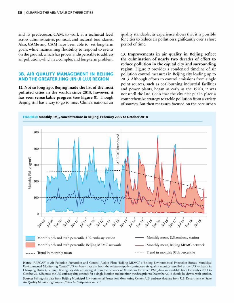
30 | CLEARING THE AIR: A TALE OF THREE CITIES
and its predecessor, CAM, to work at a technical level across administrative, political, and sectoral boundaries. Also, CAMe and CAM have been able to set long-term goals, while maintaining flexibility to respond to events on the ground, which has proven indispensable to address air pollution, which is a complex and long-term problem.
3B. AIR QUALITY MANAGEMENT IN BEIJING AND THE GREATER JING-JIN-JI (JJJ) REGION
12. Not so long ago, Beijing made the list of the most polluted cities in the world; since 2013, however, it has seen remarkable progress (see Figure 8). Though Beijing still has a way to go to meet China’s national air
quality standards, its experience shows that it is possible for cities to reduce air pollution significantly over a short period of time.
13. Improvements in air quality in Beijing reflect the culmination of nearly two decades of effort to reduce pollution in the capital city and surrounding region. Figure 9 provides a condensed timeline of air pollution control measures in Beijing city leading up to 2013. Although efforts to control emissions from single point sources, such as coal-burning industrial facilities and power plants, began as early as the 1970s, it was not until the late 1990s that the city first put in place a comprehensive strategy to tackle pollution from a variety of sources. But then measures focused on the core urban
Notes: “APPCAP” = Air Pollution Prevention and Control Action Plan; “Beijing MEMC” = Beijing Environmental Protection Bureau Municipal Environmental Monitoring Center.” U.S. embassy data are from the reference-grade continuous air quality monitor installed at the U.S. embassy in Chaoyang District, Beijing. Beijing city data are averaged from the network of 37 stations for which PM2.5 data are available from December 2013 to October 2018. Because the U.S. embassy data are only for a single location and monitor, the data prior to December 2013 should be viewed with caution.Source: Beijing city data from Beijing Municipal Environmental Protection Monitoring Center; U.S. embassy data are from U.S. Department of State Air Quality Monitoring Program, “StateAir,” http://stateair.net/.
FIGURE 8: Monthly PM2.5 concentrations in Beijing, February 2009 to October 2018
500
400
300
200
100
0
Jan 09
Jan 10
Jan 11
Jan 12
Jan 13
Jan 14
Jan 15
Jan 16
Jan 17
Jan 18
Jul 09
Jul 10
Jul 11
Jul 12
Jul 13
Jul 14
Jul 15
Jul 16
Jul 17
Jul 18
Mon
thly
PM
2.5 (μ
g/m
3 )
APP
CA
P in
trod
uced
Monthly 5th and 95th percentile, U.S. embassy station
Monthly 5th and 95th percentile, Beijing MEMC network
Trend in monthly mean Trend in monthly 95th percentile
Monthly mean, U.S. embassy station
Monthly mean, Beijing MEMC network

CLEARING THE AIR: A TALE OF THREE CITIES | 31
FIGURE 9: Timeline of air quality management actions in Beijing, 1998-2013
1998 1999 2000 2001 2002 2003 2004 2005 2006 2007 2008 2009 2010 2011 2012 2013
Source: Reproduced from UNEP (2016).
2003-2013 - Conversion to electric heating and energy efficiency retrofits in old single-story houses in core urban districts
1998-2002Replacement with electricity for selected old one-storey houses
1999/1-2002/12 China 1
1999/1-2002/12 China I
2003/12005/6 <500 ppm
2003/12005/6 <500 ppm
2001-2003 Transition
1999- CNG public buses
2008/10-Driving restriction on light-duty passengers cars
2011- License control
2011-expanded to older vehicles
2009-Subsidized scrappage of yellow-labelled vehicles
Oddeven restrictions, ban on yellow-labelled vehicles, reducing use of government-owned vehicles
Pre-2008 - 27 monitors in city, PM10 monitoring begins
2001 – public air quality forecasting begins
2012 – AQI forecasting under new national standards
2013 –35 stations with continuous PM2.5, all data made public
2009-New energy vehicles promoted by the “Ten City & Thousand Units” programme
2012- LNG buses
2013- On Road RS3
2003- Full implementation of ASM and lug down methods
2003-Yellow-labelled vehicles 2004-Freight trucks and motorcycles
2005/6-2007/12 <150 ppm
2005/6-2007/12 <350 ppm
2008/1-2012/5 <50 ppm
2001/72012/5 <50 ppm
2012/5- <10 ppm
2012/5- <10 ppm
2003/1-2005/12 China II
2005/12-2008/2 China III
2003/1-2005/12 China 2
2005/12-2008/2 China 3
2008/3-2013/1 China 4
2008/7- China IV1.2
2013/2- Beijing 5
2013/2- Beijing V1
Emission standards
1998-2010 Dedusting
retrofit
1998-2002Renovation of small boilers
in core areas
2003-2008 Renovation of coal-fired boilers (capacity below 14 MW) in
core areas
2009-2012 Renovation of coal-fired boilers (capacity over 14 MW) in six
urban districts
2006-2009Centralized heating supply centers
in rural districts/counties
2000-2006 Desulfurization
retrofit
2005- Coal to gas
2007 Denitrification
retrofit
2010- Natural gas thermal-power
cogeneration centres
Coal-fired boilers
Residential heating
Light – duty gasoline vehicles
Heavy – duty diesel vehicles
Improve gasoline quality Uncleaded Reducing
gasoline sulfur since 1998 contentImprove diesel
quality
I/M programmes and in-use inspections
Traffic restrictions on specific in-use fleets
Clean energy and new energy vehicles
Traffic management and economic measures
Temporary measures for the Olympic Games
Air quality monitoring and forecasting
Power plants

32 | CLEARING THE AIR: A TALE OF THREE CITIES
districts of Beijing, gradually expanding to cover other parts of Beijing Municipality.28 They had limited success because a large share of ambient PM2.5 pollution in Beijing originated from other areas in the Jing-Jin-Ji (JJJ) region (see Figure 11), which apart from the municipality of Beijing also includes the municipality of Tianjin, the province of Hebei, and small parts of Henan, Shanxi, inner Mongolia, and Shandong. Since 2013, with the support of the national government and line ministries, Beijing and the other cities in the JJJ have worked in coordination to tackle sources of emissions across the region, irrespective of administrative jurisdiction.
14. The year 2013 in fact marked a shift in strategy in the fight against pollution in Beijing and the JJJ region, signaled by the intervention of the State Council, China’s highest governmental body. A
year earlier, the Ministry of Environmental Protection (MEP)29 had issued new ambient air quality standards and ordered cities in the JJJ and other key regions to begin publicly monitoring PM2.5 in accordance with the new standards (MEP 2012b).30 Then, in January 2013, Beijing and much of eastern and northern China experienced several weeks of severe pollution, with concentrations of PM2.5 reaching levels similar to those experienced in Delhi during November 2017 (see Figure 10). Following this episode, in September 2013, the State Council issued the national-level Air Pollution Prevention and Control and Action Plan (APPCAP) for 2013 to 2017. The APPCAP set a target for Beijing to reduce mean annual concentrations of PM2.5 to around 60 µg/m3 in 2017 (that is, about 33 percent), while calling for the rest of the JJJ region to reduce mean annual PM2.5 by around 25 percent.
Notes: Notes: data are for illustrative purposes only; measurements are obtained by different instruments and have not been calibrated or adjusted according to a common standard or reference conditions.Sources: hHourly monitoring data from U.S. Embassy in Beijing, U.S. Department of State Air Quality Monitoring Program, http://www.stateair.net/; daily monitoring data from the Central Pollution Control Board for four stations in central New Delhi (Mandir Marg, Shadipur, Punjabi Bagh, and ITO), http://www.cpcb.gov.in/CAAQM/mapPage/frmdelhi.aspx?stateID=6
FIGURE 10: Daily average PM2.5 concentrations during severe pollution episodes in Beijing (January 2013) and New Delhi (November 2017)
0 101 Jan
11 Feb
11 Oct
600
400
200
0
19 Nov
29 Jan, 430 μg/m3
12 Nov, 499 μg/m3
8 Nov, 576 μg/m38 - 12 Jan, 569 μg/m3
24-h
our m
ean
PM2.
5 (μ
g/m
3 )
20Day
New Delhi, 2017 Beijing, 2013
30 40
28 The downtown area includes East City District, West City District, Haidian District, Chaoyang District, Fengtai District, and Shijingshan District. These, along with peri-urban districts and counties, make up Beijing Municipality
29 In 2018, the MEP went through a milestone institutional reform to be the Ministry of Ecology and Environment (MEE). 30 The MEP order applied to cities at the prefecture level and above, which correspond roughly with districts in India.
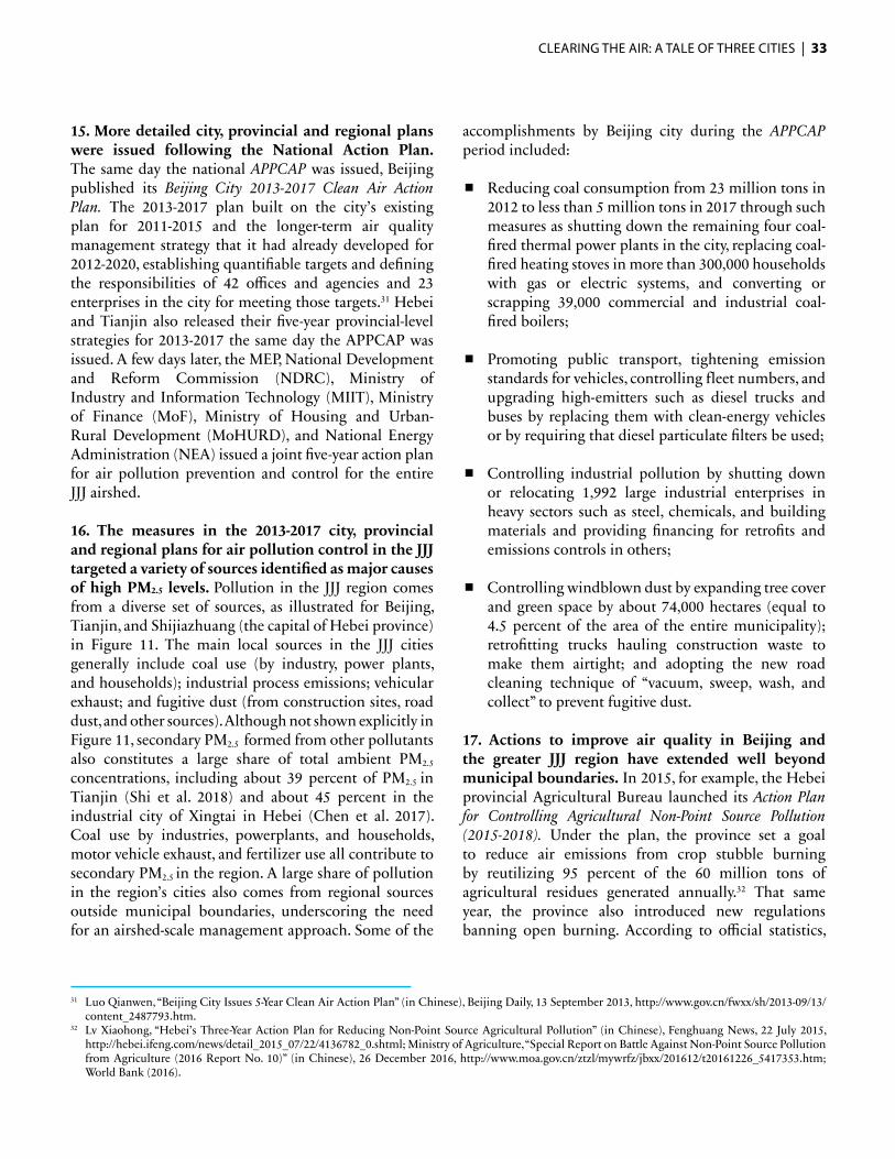
CLEARING THE AIR: A TALE OF THREE CITIES | 33
15. More detailed city, provincial and regional plans were issued following the National Action Plan. The same day the national APPCAP was issued, Beijing published its Beijing City 2013-2017 Clean Air Action Plan. The 2013-2017 plan built on the city’s existing plan for 2011-2015 and the longer-term air quality management strategy that it had already developed for 2012-2020, establishing quantifiable targets and defining the responsibilities of 42 offices and agencies and 23 enterprises in the city for meeting those targets.31 Hebei and Tianjin also released their five-year provincial-level strategies for 2013-2017 the same day the APPCAP was issued. A few days later, the MEP, National Development and Reform Commission (NDRC), Ministry of Industry and Information Technology (MIIT), Ministry of Finance (MoF), Ministry of Housing and Urban-Rural Development (MoHURD), and National Energy Administration (NEA) issued a joint five-year action plan for air pollution prevention and control for the entire JJJ airshed.
16. The measures in the 2013-2017 city, provincial and regional plans for air pollution control in the JJJ targeted a variety of sources identified as major causes of high PM2.5 levels. Pollution in the JJJ region comes from a diverse set of sources, as illustrated for Beijing, Tianjin, and Shijiazhuang (the capital of Hebei province) in Figure 11. The main local sources in the JJJ cities generally include coal use (by industry, power plants, and households); industrial process emissions; vehicular exhaust; and fugitive dust (from construction sites, road dust, and other sources). Although not shown explicitly in Figure 11, secondary PM2.5 formed from other pollutants also constitutes a large share of total ambient PM2.5
concentrations, including about 39 percent of PM2.5 in Tianjin (Shi et al. 2018) and about 45 percent in the industrial city of Xingtai in Hebei (Chen et al. 2017). Coal use by industries, powerplants, and households, motor vehicle exhaust, and fertilizer use all contribute to secondary PM2.5 in the region. A large share of pollution in the region’s cities also comes from regional sources outside municipal boundaries, underscoring the need for an airshed-scale management approach. Some of the
accomplishments by Beijing city during the APPCAP period included:
< Reducing coal consumption from 23 million tons in 2012 to less than 5 million tons in 2017 through such measures as shutting down the remaining four coal-fired thermal power plants in the city, replacing coal-fired heating stoves in more than 300,000 households with gas or electric systems, and converting or scrapping 39,000 commercial and industrial coal-fired boilers;
< Promoting public transport, tightening emission standards for vehicles, controlling fleet numbers, and upgrading high-emitters such as diesel trucks and buses by replacing them with clean-energy vehicles or by requiring that diesel particulate filters be used;
< Controlling industrial pollution by shutting down or relocating 1,992 large industrial enterprises in heavy sectors such as steel, chemicals, and building materials and providing financing for retrofits and emissions controls in others;
< Controlling windblown dust by expanding tree cover and green space by about 74,000 hectares (equal to 4.5 percent of the area of the entire municipality); retrofitting trucks hauling construction waste to make them airtight; and adopting the new road cleaning technique of “vacuum, sweep, wash, and collect” to prevent fugitive dust.
17. Actions to improve air quality in Beijing and the greater JJJ region have extended well beyond municipal boundaries. In 2015, for example, the Hebei provincial Agricultural Bureau launched its Action Plan for Controlling Agricultural Non-Point Source Pollution (2015-2018). Under the plan, the province set a goal to reduce air emissions from crop stubble burning by reutilizing 95 percent of the 60 million tons of agricultural residues generated annually.32 That same year, the province also introduced new regulations banning open burning. According to official statistics,
31 Luo Qianwen, “Beijing City Issues 5-Year Clean Air Action Plan” (in Chinese), Beijing Daily, 13 September 2013, http://www.gov.cn/fwxx/sh/2013-09/13/content_2487793.htm.
32 Lv Xiaohong, “Hebei’s Three-Year Action Plan for Reducing Non-Point Source Agricultural Pollution” (in Chinese), Fenghuang News, 22 July 2015, http://hebei.ifeng.com/news/detail_2015_07/22/4136782_0.shtml; Ministry of Agriculture, “Special Report on Battle Against Non-Point Source Pollution from Agriculture (2016 Report No. 10)” (in Chinese), 26 December 2016, http://www.moa.gov.cn/ztzl/mywrfz/jbxx/201612/t20161226_5417353.htm; World Bank (2016).

34 | CLEARING THE AIR: A TALE OF THREE CITIES
Source: figures reproduced from ICCS (2018)
a. Beijing city, 2012-2013
b. Tianjin city, 2012-2013
c. Shijiazhuang city, Hebei province, 2013-2014
FIGURE 11: Sources of PM2.5 pollution in cities in the JJJ region
region transmission 28%-36%
local pollution emissions 64%-72%
local pollution emissions
coal combustion
industrial production
motor vehicles
dust
other
22.4%14.1%
14.3%
31.1%18.1%
region transmission 22%-34%
local pollution emissions 66%-78%
local pollution emissions
coal combustion
industrial production
motor vehicles
dust
other
27%
6%
30%
20%
17%
region transmission 23%-30%
local pollution emissions 70%-77%
local pollution emissions
coal combustion
industrial production
motor vehicles
dust
other
28.5%
8.8%
22.5%
15.0% 25.2%

CLEARING THE AIR: A TALE OF THREE CITIES | 35
by 2017 the reutilization rate for agricultural residues had reached 96 percent, with most being returned to the field to enhance soil nutrient content or being used for animal feed. Still, provincial authorities report that enforcement continues to be a problem and burning has continued in some areas.33 In addition, to tackle generation of secondary PM2.5, the local government in Hebei initiated a pilot program (under the World Bank supported Hebei AQM Program for Results (P4R) project) to increase Nitrogen Use Efficiency (NUE) on 6.2 million hectares of farmland that will reduce NH3 through balanced fertilizer application. This pilot is expected to be further expanded to other parts of China. China is also: (i) piloting the use of covered tanks for storage of animal manure to minimize NH3 emission on large livestock farms; (ii) applying technologies that ensure that fertilizer is injected sufficiently into the soil on large farms for both crop and vegetable production; and (iii) developing new plasma reactor technology that transforms manure from liquid to solid form prior to being used on farmland.
18. The central government has provided dedicated financial resources to support implementation of pollution control strategies in the JJJ region. All told, between 2013 and 2017, direct outlays by the central government totaled RMB 52.8 billion (US$ 7.81 billion) in special-purpose funds and RMB 10 billion (US$ 1.48 billion) in budgetary resources to support air quality management in the JJJ provinces.34 In 2016, for example, Hebei province received earmarked resources of about RMB 4.01 billion (US$ 593 million) from the central government plus RMB 902 million (US$ 130 million) in transfers from Beijing and Tianjin cities, while committing RMB 800 million (US$ 120 million) in specially designated provincial resources to implement its air pollution control plan.35 The province used these
resources to leverage an additional RMB 20 billion (US$ 2.96 billion) in financing from the private sector.
19. Financing from the central government and city for air pollution control in Beijing has supported a variety of incentive programs. Examples of incentive programs include:
< Subsidies for end-of-pipe controls and boiler retrofits in power plants and factories: Since 2004, the national government has offered coal-fired power plants a price subsidy to offset the increased marginal cost of installing and operating end-of-pipe controls.36 Smaller industries have also received incentives for installing control technologies and lower-emissions equipment. In 2017, businesses retrofitting small boilers (steam capacity up to 20 tons) to reduce NOx emissions could receive subsidies from the city of RMB 96,000 to RMB 580,000 depending on the size of the boilers. District governments in the city were expected to offer matching subsidies.37
< Cash for clunkers: By 2015, Beijing had already banned the worst-polluting vehicles from entering the city.38 Additionally, it offered cash incentives for owners with vehicles that had been registered for at least 6 years to scrap their older vehicles. The incentives ranged from RMB 3,500 (US$ 518) for small passenger vehicles to RMB 21,500 (US$ 3,180) for large buses. Vehicle owners had to dispose of their vehicles at least a year ahead of the mandatory retirement date, if applicable (e.g. for example, for public buses), in order to receive the subsidy. The city has also offered subsidies to encourage drivers to purchase clean-energy vehicles. In 2017, for example, drivers could receive RMB 44,000 (US$ 6,509) in national subsidies plus RMB 22,000 (US$ 3,254) in
33 Ministry of Agriculture, “Hebei Maintains Reutilization Rate for Agricultural Residue above 96%,” 5 June 2017, http://www.moa.gov.cn/ztzl/2017sxsc/sxdt/201706/t20170605_5660829.htm; Sohu News, “Reutilization Rate for Agricultural Residues Reaches 96% This Year, Still a Structural Problem” (in Chinese), 4 December 2017, http://www.sohu.com/a/208280431_115479.
34 Data on central government support for air pollution control are from remarks by Liu Bingjiang, MEP Atmospheric Division Chief, GoC, “Responses from Ministry of Environmental Protection on Progress Made in Air Pollution Prevention and Control Work” (in Chinese), 27 February 2018, http://www.gov.cn/xinwen/2018-02/27/content_5269486.htm.
35 Gao Zhili, Director of Hebei Province Financing Department, “Report on the Implementation of the 2016 Budget and Drafting of the 2017 Budget in Hebei Province” (in Chinese), http://www.mof.gov.cn/zhuantihuigu/2017ysbghb/201703/t20170306_2547723.html.
36 In 2013, power plants received electricity price subsidies from desulfurization, denitrification, and dust-removal equipment of RMB 0.015/kWh, RMB 0.01/kWh, and RMB 0.002/kWh, respectively. Christopher James, “China’s Power Sector and Air Quality Reforms: Global Lessons on Getting Institutional Responsibilities Right,” 7 November 2017, https://www.raponline.org/knowledge-center/chinas-power-sector-air-quality-reforms-global-lessons-getting-institutional-responsibilities-right/?sf_action=get_data&sf_data=results&_sft_region=china&_sft_language=english.
37 Beijing, Sanhui Heating and Environmental Technology Development Company, Limited, “Beijing City Subsidy Policies for Low-Nitrogen Retrofits of Boilers” (in Chinese), http://www.bjshnh.com/gaizao/91.html.
38 Called “yellow-label” vehicles for the color of their emissions stickers, these included gasoline vehicles that failed to meet the China I standard and diesel vehicles that could not meet the China III standard.

36 | CLEARING THE AIR: A TALE OF THREE CITIES
subsidies from Beijing city for buying all-electric vehicles.39
< Household subsidies for clean heating: By October 2017, Beijing had imposed a total ban on coal use by households for cooking and heating within city limits, including in peri-urban villages. To help families make the switch, the city heavily subsidized the purchase of new boilers and stoves and lowered the price of energy for heating. Households in rural areas switching to electric heating, for example, could receive RMB 24,000 (US$ 3,550) in subsidies for a new heating system, reducing the upfront cost per household to around RMB 3,000 (US$ 444). Additionally, they enjoyed a lower tariff rate for electricity use during winter nights, reducing the average winter heating cost per household to around RMB 1,661 (US$ 246). By comparison, the average winter heating cost for a household burning coal would have been around RMB 5,000 (US$ 740).40
20. Cross-jurisdictional coordination on air pollution control in the JJJ region has been led by the State Council and the JJJ Regional Air Quality Prevention and Control Coordination Group, with high-level participation. Provincial and city-level governments continued to be the primary implementers for air quality management in the JJJ region. At the same time, the JJJ Regional Air Quality Prevention and Control Coordination Group was established in 2013 to ensure cross-jurisdictional coordination. Originally housed in the Beijing Environmental Protection Bureau, the group included representatives from seven provinces and municipalities and eight ministries under the State Council, with the Vice Premier serving as its head. Mirroring the regional group, multi-agency leadership groups were also established at the provincial and local levels of government. The ministries and provinces in the regional coordination group formulated annual implementation plans for air quality management in the JJJ region and set policies for cross-jurisdictional
issues such as fuel standards, energy supply, and public transportation.41 In July 2018, the State Council decided to further elevate the administrative status of the coordination group, with the Minister of Ecology and Environment (MEE), Beijing City Governor, Tianjin City Governor, and Hebei Provincial Governor now acting as its vice-chairs. Other members now include vice- ministers from the NDRC, MIIT, Ministry of Finance, Public Security Administration, Ministry of Housing and Urban Development, Ministry of Transportation, Ministry of Agriculture, Chinese Meteorological Administration, and other agencies. The Secretariat is expected to sit within the national-level MEE (formerly MEP).42
21. Local government officials and state-owned-enterprise managers were held accountable for implementing air quality management plans by integrating air quality targets and measures into official performance reviews. In 2014, the State Council issued rules for evaluating the performance of government officials in carrying out the responsibilities defined in the local-level air pollution prevention and control plans.43 Per the rules, officials failing to meet the 2017 targets would be ordered to appear before the State Council, and approvals for new development projects in their area would be suspended. The rules also made the achievement of air quality targets a more integral part of official cadre performance reviews. China’s government first started to embed environmental targets in the system for evaluating cadres in the early 2000s. The annual reviews can determine bonuses and an official’s prospects. Although far from perfect (see Kostka, 2015), the reviews have become an influential lever in shaping official behavior (Wang, 2013). Officials that consistently fail to meet targets may be demoted, reassigned to a less prestigious locality, or possibly expelled (Eaton and Kostka, 2014). In the closing months of the APPCAP, the MEP announced that it had disciplined 12,000 officials.44 The government has taken continuous efforts to refine policies. For example, to enhance environmental
39 Subsidy amounts are for an all-electric vehicle with a range of greater than 250 km. Beijing People’s Government, “Beijing City Subsidy for New Energy Vehicles Set at 50% of National Subsidy, Maximum of RMB 44,000” (in Chinese), 10 February 2017, http://www.beijing.gov.cn/bmfw/zxts/t1468354.htm.
40 Xinhua, “Beijing Resolutely Switches from Coal to Electric Heating” (in Chinese), 22 April 2017, http://www.xinhuanet.com/politics/2017-04/22/c_1120854758.htm; He Cong, Jia Yong, Xi Bo, Wan Jintao, “Another Heating Season Arrives, How Can the North Have Heat While Also Having Good Air?” (in Chinese), People’s Daily, 15 November 2017, http://www.bjd.com.cn/sd/hcr/201711/15/t20171115_11074943.html.
41 Beijing Environmental Protection Bureau Press Office, “Air Pollution Prevention and Control Work in the Expanded Jing-Jin-Ji Region” (in Chinese), 24 July 2014, http://bjepb.gov.cn/bjhrb/xxgk/jgzn/jgsz/jjgjgszjzz/xcjyc/xwfb/607628/index.html.
42 General Office of State Council, Notice of General Office of the State Council Regarding the Formation of the Leading Group for Air Pollution Prevention and Control in the Extended Jing-Jin-Ji Region, 11 July 2018, http://zhengce.beijing.gov.cn/library/192/33/50/438650/1558190/index.html.
43 State Council, “Notice of the General Office of the State Council on the Issuances of Rules for Evaluation of Implementation of the Air Pollution Prevention and Control Plan” (in Chinese), 30 April 2014, http://www.gov.cn/zhengce/content/2014-05/27/content_8830.htm.

CLEARING THE AIR: A TALE OF THREE CITIES | 37
44 Nectar Gan, “12,000 Officials Disciplined and 18,000 Companies Punished in China’s Sweeping Crackdown Against Pollution,” South China Morning Post, 2 September 2017, https://www.scmp.com/news/china/policies-politics/article/2109342/top-level-china-pollution-inspections-wrapping.
45 By some estimates, better-than-usual atmospheric circulation and other favorable weather conditions contributed about 30 percent to the reduction in mean PM2.5 in 2017 compared to 2013. Li He, “Air Quality Takes a Turn for the Better in the Jing-Jin-Ji Region – Experts Credit More Focused, Targeted Pollution Control Efforts” (in Chinese), Xinhua, 28 February 2017, http://www.xinhuanet.com/energy/2018-02/28/c_1122463587.htm.
46 Hebei News, “PM2.5 Concentrations Drop 8%! Target Fixed for Xingtai to Improve Air Quality in 2018” (in Chinese), 27 April 2018, http://hebei.hebnews.cn/2018-04/27/content_6863379.htm.
47 Other Central Acts (Water, Environment Protection, Motor Vehicles, and Public Liability) also have provisions to regulate air quality (CSE 2016).
performance accountability at the city level, provinces such as Hebei and Shanxi introduced a transparent fiscal budget reward and penalty scheme to take account of municipal Air Quality Index (AQI), PM2.5, PM10 and SO2 concentrations levels using a formula.
22. Regulatory changes and greater openness in the public dissemination of environmental data have also helped improve government accountability for air quality. Rules promulgated by the MEP have required that they make their environmental monitoring data public, and near-real-time data on air quality is now available for most cities and stations. The government has also required continuous emissions monitors to be installed in large industrial facilities and for the data from these facilities to be made public.
23. The JJJ region made tremendous progress in reducing PM2.5 pollution during the APPCAP period, finally bending the curve on rising concentrations. Average PM2.5 concentrations in Beijing exhibit a distinct drop beginning around September 2013, as the city reduced its mean annual PM2.5 from around 90 µg/m3 to 58 µg/m3 in 2017 (see Figure 8). Severe pollution episodes have also abated. Mean annual PM2.5 in the larger JJJ region dropped by nearly 40 percent, far exceeding the APPCAP target of 25 percent.45 Some cities in the JJJ region achieved even larger declines, including the industrial center of Xingtai in Hebei province, which had some of the worst pollution in the country at the start of the APPCAP. Mean annual PM2.5 in Xingtai declined from 160 µg/m3 in 2013 to just below 80 µg/m3 in 2017.46
24. Much remains to be done before the cities will reach compliance with the national standards, however. By early 2018, average levels of PM2.5 in the JJJ remained about two times higher than the national standard and seven times higher than the guideline value recommended by the WHO. To continue the momentum of the APPCAP, in August 2018 the State Council issued the Three-Year Action Plan to Win the Battle for Clean Skies in 2018 to 2020. Beijing, Hebei, Tianjin, and other local governments in the JJJ region have followed
closely with their own three-year strategies. As air quality continues to improve, many of the cheapest no-regrets solutions have already been taken, and the challenge for the next round of air pollution management will be for the governments in the JJJ to analysis and identify measures that deliver the greatest reduction in exposure at the least cost to the economy. Furthermore, innovative financing mechanisms and private sector investments will need to be mobilized to sustainably finance air quality management for the long term.
3C. AIR QUALITY MANAGEMENT IN DELHI
25. There is a long history of tackling air pollution in India, with supporting legislation. The main legislation that governs air pollution management in India is the Air (Prevention and Control of Pollution) Act (“Air Act”), first issued in 1981 and amended in 1987.47 The Air Act empowers the Ministry of Environment, Forest, and Climate Change (MoEFCC), and its subordinate institutions, Central Pollution Control Board (CPCB) and the state pollution control boards (SPCBs), to perform a range of functions to help prevent, control, and abate air pollution in the country. CPCB, for example, has the responsibility to prescribe air quality standards, the first set of which were issued in 1984 and have been since been expanded and strengthened. Additionally, the Air Act requires CPCB and SPCBs to develop nationwide programs and state-level plans, respectively, to help achieve ambient air quality standards. Program and plan implementations are left to state governments, however.
26. Pollution control boards also have powers to prescribe and enforce emission standards for stationary and mobile source of air pollution, in coordination with other government agencies. For stationary sources of pollution – industrial plants and thermal power plants, for example -- India relies on an emission-standards-and-permit system. Emission standards for different categories of industry (including power plants) have been established, and facilities must obtain permits to establish and operate, that, in turn, allows regulators to enforce the set standards (see

38 | CLEARING THE AIR: A TALE OF THREE CITIES
Box 3). Regulators also monitor emission levels and have the authority to shut down or disconnect water or power to non-compliant units. Fines and imprisonment can be pursued through courts. For mobile source of pollution, vehicles, as in much of the world, India relies on emission standards for newly manufactured vehicles along with fuel quality standards. Vehicle inspection and maintenance (I and M) programs are used for in-use vehicles. Central Motor Vehicles Rules of 1989 grants the Ministry of Road Transport and Highways (MoRTH) the responsibility to establish vehicle specifications. Therefore, standards for vehicles and I and M program are developed jointly by MoEFCC and MoRTH. Ministry of Petroleum and Natural Gas (MoPNG) and the Bureau of Indian Standards are in charge of setting standards for quality of gasoline and diesel in the country. Furthermore, MoRTH enforces vehicular
emission standards, MoPNG fuel quality standards, and state police and state transport departments enforce I and M programs. In critically polluted areas (including non-attainment cities), pollution boards can also prohibit the use of certain fuels and burning of any materials deemed to cause air pollution and mandate the use of certain pollution control equipment. For example, use of pet coke and furnace oil has been restricted in Delhi and the National Capital Region (NCR), and brick kilns are required to use prescribed technologies to reduce air pollution in this area. This provision also allows SPCBs to restrict trash burning in non-attainment areas.
27. Based on this legislation, but driven by public interest litigation and public pressure, Delhi began to tackle air pollution starting in the mid-1980s. Air pollution started to deteriorate in Delhi beginning in
BOX 3: Controlling Air Pollution from Coal-Fired Power in India
India has made great strides in extending access to electricity to its people. In 1990, only 43 percent of the population had some form of access to electricity. By 2016, that number had risen to nearly 85 percent.48 Still, about 25 million rural households continue to be unconnected,49 and per capita consumption of electricity in India in 2016 was less than a quarter that of the other BRICS countries, at 916 kWh compared to 4,262 kWh. The power sector in India has ample room to grow, and demand is expected only to rise.
Coal has largely fueled India’s expanding access to electricity and will continue to do so in the coming decades. By the end of 2018, India’s power utilities had 197 gigawatts (GW) of installed coal-fired capacity, out of a total generating capacity of 347 GW, as the share of coal-fired generation in India’s total electricity supply reached 78 percent (see Figure B3.1). Separately, industries operated another 57 GW of captive thermal generating capacity
48 World Bank, “Access to Electricity (% of population)” (EG.ELC.ACCS.ZS), World Development Indicators database.49 Bhasker Tripathi, “15 Million Indian Households Have Meters But No Electricity,” Bloomberg, 1 November 2018, https://www.bloombergquint.com/
global-economics/15-million-indian-households-have-meters-but-no-electricity#gs.tUw7ok1D.
Notes: The data include generation by utilities and exclude captive generation by industries.Sources: 1980-2014 data from IEA (2018b); 2015-18 data from India’s Central Electricity Authority (CEA) and Indiastat
FIGURE B3.1: Share of coal-fired power in total electricity generation in India, 1980-2018
85807570656055
Elec
tric
ity g
ener
ated
from
coa
l (%
tota
l)
504540
1980
1982
1984
1986
1988
1990
1992
1994
1996
1998
2000
2002
2004
2006
2008
2010
2012
2014
2016
2018

CLEARING THE AIR: A TALE OF THREE CITIES | 39
50 Projections are for the “New Policies Scenario” in IEA’s World Energy Outlook 2018 (IEA 2018a).51 Densely populated areas include areas with more than 400 people per square kilometer. Manka Behl, “Supreme Court to 57 Power Plants: Clean Up Act
within 28 Months,” TNN, 11 September 2018, https://timesofindia.indiatimes.com/city/nagpur/supreme-court-to-57-power-plants-clean-up-act-within-28-months/articleshow/65761232.cms.
TABLE B3.1: Power Plant Emissions Standards in Various Countries
Notes: Existing plants refer to plants in operation as of when the respective standards were issued; new plants are plants that enter operation after the respective dates that the standards were issued or entered into force; the date of issue varies by region/country; the ranges shown in the table depend on the size, type, age, and location of the plant as per the standards for the respective countries/regions shown in the table; averaging or sampling periods vary; standards for the United States and Japan have been converted into units of µg per Nm3 by Zhu and Wang (2014); standards for China shown in the table are for the 11 provinces in the eastern region; standards for the EU shown in the table apply to a plant with a generating capacity of 300 MW to 1 GW and are effective as of 2021; all other standards are currently in effect.Sources: Zhang (2016) and EU (2017)
for their own use. The International Energy Agency projects that, by 2040, the share of coal in total generation will drop to just below half, as India’s electricity mix becomes more diversified. Still, coal will continue to be the single largest fuel source, and, in absolute terms, coal-fired generation will be about twice what it was in 2017.50
Although expanding access to electricity has improved the lives of hundreds of millions of people, the growing reliance on coal-fired generation has also come at a cost. Coal-fired power is a major source of air pollutant emissions.
Amid growing public concern over pollution, in 2015 the Ministry of Environment, Forest and Climate Change (MoEFCC) introduced new standards for emissions from thermal power plants, which were amended in 2018. The new standards restricted SO2, NOx, and mercury (Hg) emissions for the first time and tightened the existing limits on PM emissions. The new standards were comparable to those in other countries although above the limits currently achievable with the best available technologies (see Table B3.1). The MoEFCC set a deadline for power plants to comply with the standards by the end of 2017. The deadline was later extended to 2019 for Delhi and to 2022 for all other states and UTs. India’s Supreme Court has called for the government to implement the new standards by 2021 for 57 generating units located in India’s most densely populated areas.51 As of mid-2018, only 15 out of 650 units had installed emissions controls capable of meeting the new standards for SO2, and 273 units were in non-compliance with the PM standards. While some of the non-compliant units are older and will be retired, more than 410 units will need to be retrofitted with SO2 controls and over 230 units will need to have their PM controls upgraded to meet the 2022 deadline (CEA 2018). A range of viable technologies exist to control SO2, NOx, and PM before, during, and after combustion Pre-combustion controls include coal washing, which reduces the content ash and other impurities and improves the heating value of coal. During-combustion controls include optimizing the temperature, burn time, and boiler load and injecting sorbents such as limestone into the ame zone of the boiler. Post-combustion controls
Existing plants New plantsNOx SO2 PM2.5 NOx SO2 PM2.5
China (2014) 100 50-200 20-30 50 35 10India (2015) 300-600 200-600 50-100 100 100 30Japan (2015) 410 100 200 200 50South Africa (2012) 1,100 3,500 100 750 500 50
USA (2014) 135 185 18.5 95.3 136 12.3
EU (2017) 165-220 (daily)65-85 (annual)
165-220 (daily)130-180 (annual)
11-20 (daily)8-12 (annual)
125 (daily)85 (annual)
110 (daily)75 (annual)
10 (daily)5 (annual)

40 | CLEARING THE AIR: A TALE OF THREE CITIES
include end-of-pipe technologies to capture or remove pollutants from f lue gas. Examples of new technologies to emerge in recent years include f lue gas conditioning, enhanced ESP, better fabric filters, agglomeration (binding small particles together to make them easier to capture), and hybrid systems (Zhang, 2016). In parallel with emissions controls, installing continuous emissions monitoring (CEM) equipment and making CEM data publicly available can improve compliance by ensuring that companies operate within standards and that the most egregious violators are held accountable.
The MoEFCC has prescribed specific pollution control equipment for power plants to meet the new standards. New PM emission standards are to be met through the augmentation of ESP, f lue gas desulphurization to control SO2 is recommended as are post combustion measures like selective catalyst reduction and selective non-catalyst reduction systems for more stringent NOx standards. On its part, the Ministry of Power has taken measures to remove existing hurdles in the implementation of the new emission standards. The Central Electricity Authority, for example, has issued standard technical specifications for wet limestone-based f lue gas desulphurization for a typical 500 MW unit which can readily be used by the utilities.
Retrofitting thermal power plants with emissions control technologies can be technically challenging and expensive. Power producers will need to recoup the costs of putting in place control measures by raising tariffs. Ultimately, accelerating the retirement of older plants while promoting more renewable energy and energy efficiency may prove more cost-effective, allowing India to reduce harmful emissions from the power sector and avoid the lock-in effects that may also increase climate mitigation costs down the road.52 As part of its commitment to global climate change mitigation efforts, the Government of India has set an ambitious target of meeting energy demand through 175 GW of renewable energy.
52 Authors’ email correspondence with Gailius Draugelis, World Bank Lead Energy Specialist, February 2019.
the 1980s. In 1985, public interest lawyer, M.C. Mehta, asked the Supreme Court of India to direct government agencies and departments to implement the Air Act in Delhi. The Supreme Court has been granted the authority to hear cases that infringe on a citizen’s fundamental rights that are guaranteed under Article 21 of the Indian Constitution. Right to a clean environment is one such fundamental right. Spurred by the case, the Supreme Court began to push not only the Delhi government, but also the Central government, to take measures to improve Delhi’s air quality.
28. Over the course of the next decade and a half, a number of measures were implemented based on the push from the Supreme Court and pressure from the public, that brought some temporary relief from poor air quality. In the 90s, emissions from transport were understood to contribute 60-70 percent of the total, with the rest coming from industry and residential sources; sources were understood to be located within the city boundaries. As a result, most measures to reduce air pollution in Delhi focused on transportation (see Table 6). Between 1994 and 1998, the Court pushed the
government to enforce the phaseout of leaded gasoline, to introduce pre-mix fuels for two-stroke engines, relocate polluting industries, and implement scrapping of commercial vehicles in use for 15 years or more. The Delhi government and MoEFCC developed their first comprehensive plans for controlling pollution in 1996 and 1997, respectively, on the Court’s urging. The Delhi government plan called for a Mass Rapid Transport System, a highway bypass around Delhi, improved vehicular technology, higher-quality fuels, increased use of CNG, restrictions on excessively polluting vehicles, urban greening, and a program of public awareness. The MoEFCC plan was similar and focused on transport. The Court subsequently asked for a committee to be established to monitor the progress on implementation and to suggest other policies to control pollution. This committee was called the Environment Pollution (Prevention and Control) Authority (EPCA). Soon after, based on a report from EPCA, the Court mandated that all commercial vehicles switch to CNG by 2001. This order initiated one of the most ambitious vehicular-fuel-conversion programs globally, and one that was implemented in less than two years by December 2002.

CLEARING THE AIR: A TALE OF THREE CITIES | 41
With coordinated action from a range of stakeholders -- suppliers of CNG, bus manufactures, public vehicle operators -- about 10,000 buses converted from diesel to CNG, and approximately 20,000 taxis and 50,000 three-wheelers from petrol to CNG, bringing some brief relief to Delhi’s citizens (see Figure 12).
29. Air quality, however, steadily declined in the 2000s, building up to a crisis in the late 2010s. As shown in Figure 12c, mean annual PM10 concentrations in Delhi have increased year after year from the early 2000s. The winter of 2016 brought very poor air quality to the city, with PM2.5 concentrations of up to 759 µg/m3, 12.7 times higher than the national standard (EPCA-CSE 2018), for example. Delhi has consistently featured on top in WHO’s list of most polluted cities in the world during this period.
30. Delhi’s air pollution challenge has come to be recognized as multi-sectoral and multi-jurisdictional. Over the last few years, three different source apportionment studies (Sharma et al. 2016, Amman et al. 2016, and ARAI-TERI 2018) have estimated the contribution of different sectors to seasonal (winter and summer) and mean annual ambient concentrations of PM2.5 in Delhi and the NCR. Findings from the latest of these studies --- ARAI-TERI 2018 -- are illustrated in Figure 13. These studies show that there are multiple dominant sources of pollution which require a multi-source strategy for pollution management in Delhi. Though there are differences, all three studies rank secondary inorganic aerosols (formed by reactions involving primarily NH3 from agriculture mixed with NOx and SO2); biomass (household cookstoves); waste burning; and vehicular emissions (including pollution from diesel vehicles,
Date Measure1985 Mr. Mehta petitions the Supreme Court (SC) to direct various government departments to enact the Air Act in Delhi.1986 SC directs the Delhi Government to specify what steps have been taken to reduce air pollution.
1990First set of vehicular exhaust emission standards are set (for in-use vehicles) and committee established to recommend vehicular emission standards (for new vehicles); Central Government approves Delhi Second Master Plan which calls for polluting industries to be relocated by 1993.
Early 1990 MoEFCC proposes that all vehicles have compulsory catalytic convertors by 1995.
1991 SC asks MoEFCC to establish statutory committee (under provision of Environment Protection Act (1986)) to devise policies to reduce air pollution. The Saikia Committee is established.
1992 The Saikia Committee recommends phase-out of unleaded gasoline in Delhi and use of CNG as an alternative fuel.1993 MoEFCC established vehicular emission standards to be met by 1996 and 2000.
1994 The Motor Vehicles Act is amended to encourage use of alternative fuels; SC mandates phase out of unleaded fuel in Delhi by 1995 and gradually reduction in the sulfur content of diesel by 1998. These deadlines are met.
1995 The Delhi Government announces subsidy for 2-3 wheelers to install catalytic convertors and MoRTH bans registration of 4 wheelers without catalytic convertors in Delhi. These initiatives are successful.
1996 With further deteriorations in air quality, SC orders Delhi Government to prepare a comprehensive air quality management plan.
1996-97On orders from the Supreme Court, Delhi Government relocates highly polluting industries from Delhi having missed the 1993 deadline. Delhi Government and MoEFCC present first comprehensive actions plans for air quality management.
1997 Based on its Action Plan, Delhi Government develops policy to phase- out old vehicles starting in 1998 to 2000 and encourage the use of CNG.
1998
SC orders MoEFCC to establish the third in a series of committees to monitor implementation of action plans and devise new policies. This committee is called Environment Pollution (Prevention and Control) Authority (EPCA) and is still functioning. Based on recommendations from EPCA, SC orders that all commercial passenger vehicles -- autos, taxis, and buses -- switch to CNG by 2000.
1999On orders from the Supreme Court, Delhi Government implements policy to phase out vehicles older than 15 years having missed previous deadline of 1998. Incentive scheme -- exemption from 8% sales tax and subsidy of 4% on the interest rate of the loan -- is used to incentivize conversion.
2002 SC's 1998 CNG conversion order is implemented.
TABLE 6: Timeline of key measures to tackle air pollution in Delhi in the 1990s and early 2000s

42 | CLEARING THE AIR: A TALE OF THREE CITIES
FIGURE 12: Monitored concentrations of pollutants in Delhi compared to national standards,1990-2018
b. Mean annual NO2 concentrations in Delhi NCR, 1990-2018
NAMP max annual mean
CAAQM mean, 2016-2018 (9-10 stations)
CAAQM max annual mean
NAMP mean, 1990-2017 (2-7 stations)
140
1990 1995 2000 2005 2010 2015
WHO guideline and national standard
90
100
110
120
130
80
70
60
50
40
30
20
10
0
Mea
n an
nual
NO
2 (μg
/m3 )
a. Mean annual SO2 concentrations in Delhi NCR, 1990-2018
1990 1995 2000 2005 2010 2015
National standard (2009)
20
30
40
50
60
10
0
Mea
n an
nual
SO
2 (μg
/m3 )
NAMP mean, 1990-2017 (2-7 stations) NAMP max annual mean
CAAQM mean, 2017-2018 (7 stations) CAAQM max annual mean

CLEARING THE AIR: A TALE OF THREE CITIES | 43
c. Mean annual PM10 concentrations in Delhi NCR, 2003-2018
Notes: For O3, CO, NO2, and SO2, data for 1990 to 2017 are from the manual monitoring stations in the National Ambient Air Quality Monitoring Programme (NAMP) network; for PM10, data for 2003 to 2015 are from the NAMP network; for all other years, data are from the automated stations in the Continuous Ambient Air Quality Monitoring (CAAQM) network as 2018 data were not available from the manual NAMP stations. Source: India Central Pollution Control Board, available at https://app.cpcbccr.com/ccr/#/caaqm-dashboard-all/caaqm-landing.
NAMP max annual mean
CAAQM mean, 2016-2018 (5-6 stations)
CAAQM max annual mean
NAMP mean, 2003-2017 (3-8 stations)
500
2003 2005 2007 2009 2011 2013 2015 2017
WHO guideline
National standard
450
400
350
300
250
200
150
100
50
0
Mea
n an
nual
PM
10 (μ
g/m
3 )
road dust, tire wear, and brakes) as the most important sources of pollution in the winter months. Confirming these findings, Cusworth et al. (2018) find that smoke from agricultural burning in upwind states contributed about 21-72 percent of ambient PM2.5 in Delhi during early November when the NCR frequently experiences severe pollution episodes. There is less agreement among the studies on pollution sources in the summer months, though dust and construction are likely the largest contributors. Regional sources of air pollution also contribute a large share of overall ambient PM2.5
concentrations, with as much as 60 percent of Delhi’s pollution comes from neighboring states (Amman et al. 2016).
31. Delhi has once again taken on the challenge of deteriorating air quality with EPCA continuing to play an important role. The tenure of EPCA has been extended time and again, and most recently EPCA was reconstituted in October 2018 to include a larger number of representatives from civil society. Other
members who have served longer term on EPCA include officers from Government of Delhi’s Environment Department, Transport Department, Jal (Water) Board, officials from Delhi’s four municipal corporations, and Delhi police. EPCA has continued to play a role in advising the Supreme Court in matters pertaining to air pollution management and to ensure implementation of air quality standards and related Court orders in Delhi and the NCR (MoEFCC 2018). In consultation with the Central government and relevant state governments, EPCA developed a comprehensive action plan that provides timelines for different responsible agencies to implement medium and long-term measures to tackle air pollution in Delhi NCR. This plan was subsequently notified by CPCB in 2018 per directions of the Court. The plan includes measures of reduce emissions from vehicles, power plants, industry, construction, waste burning, and solid fuels in domestic and hotel sectors. In addition, an emergency action plan – Graded Response Action Plan -- developed also by EPCA was notified in 2017 and becomes effective during high pollution

44 | CLEARING THE AIR: A TALE OF THREE CITIES
a. During winter months b. During summer months
FIGURE 13: Sources of PM2.5 pollution in Delhi NCR region, 2017-18
Source: ARAI-TERI (2018)
Delhi/NCR, 2017-2018 (winter)
motor vehicles
industry
dust
other
biomass
secondary
Delhi/NCR, 2017-18 (summer)
motor vehicles
industry
dust
other
biomass
secondary
episodes initiating costly, short-term measures to bring down pollution (EPCA 2019). For example, following the spike in air pollution on November 7, 2017, when PM2.5 concentration in Delhi was 504 µg/m3, EPCA issued directives to state governments in the Delhi NCR to close polluting industries, continue ban on generator sets, stop use of unapproved fuels and coal and firewood in eateries, among other measures to reduce dependence on private vehicles.
32. A number of measures have been implemented to improve air quality in Delhi, some at the national level and others specifically in the NCR.
< To tackle vehicular pollution: India has progressively tightened vehicular emission and fuel quality standards and has announced plans to jump from BS-IV (equivalent to ES-IV) to BS-VI (equivalent to ES-VI) from 2020, an unprecedented advancement of emission standards. Moreover, BS-VI (equivalent for ES-VI) grade fuel was made available in the National Capital Territory two years ahead of schedule.
< To tackle industrial and power plant emissions: Highly polluting fuels used in industry – petroleum coke and furnace oil – were prohibited in NCR states as per the directions issued by CPCB in November
2017. New emissions standards for eighteen categories of industries were issued in 2018 to reduce emissions of NOx and SOx in the NCR but will also contribute to better air quality nationally. The Badarpur coal-based power plants that supplied power to Delhi for over four decades was permanently shut in 2018. Additionally, brick kilns in the NCR have been ordered to move to zig-zag technology, which will substantially reduce pollution.
< To tackle agriculture residue burning: A National Policy for Management of Crop Residues was announced in 2014 and in 2018 the Cabinet Committee on Economic Affairs gave approval for the promotion of Agricultural Mechanization for in-situ Management of Crop Residue in the states of Punjab, Haryana and Uttar Pradesh, and in National Capital Territory of Delhi, in efforts to reduce large-scale burning of crop residue from paddy crop in October-November and wheat in April.
33. Delhi, and other regions in the country, will also benefit from a number of other national initiatives to tackle air pollution, and others that though not initiated for air pollution concerns will nonetheless help reduce air pollution as a co-benefit. In 2015, for example, MOEFCC introduced new emission standards

CLEARING THE AIR: A TALE OF THREE CITIES | 45
for power plants, which, once enforced, will bring benefits in terms of reduction in PM2.5 concentrations (see Box 3). In addition, seventeen categories of polluting industries have been directed to install Online Continuous Emissions/Effluent Monitoring Systems, in an effort to improve enforcement. Rules for construction and demolition waste management were issued in 2016 and five waste management rules – for solid waste, hazardous waste, plastic waste, biomedical waste, and e-waste -- revised. The National Solar Mission and National Mission on Energy Efficiency that were initiated to achieve India’s ambitious climate targets will also help shift the energy mix towards renewables and away from thermal power plants, yielding air quality improvements as a co-benefit. India is also promoting electric vehicles53 and has initiated plans to develop hydrogen as a transport fuel for the future. Programs such as the Pradhan Mantri Ujjwala Yojana that has expanded access to clean cooking fuels, most notably LPG (see Box 4), reducing the reliance on residential biomass burning, is essential to efforts to reduce air pollution. Ministry of Agriculture is also promoting programs to reduce the use of fertilizers such as Soil Health Card Scheme, which provide soil fertility status and recommendations on per crop fertilizer dose, and Integrated Nutrient Management practices. Bringing
these and other initiatives together with a concentrated focus on air pollution management, in 2019, MoEFCC also launched the National Clean Air Programme (NCAP). The NCAP has set a time-bound goal for improving air quality across the country to help around 100+ cities, where air pollution standards are currently not being met, meet standards over time. The NCAP provides cities an overall framework for developing air quality management plans and guidance on interventions across a range of sectors (power plants, transport, industry, agriculture, residential, waste management, and road and construction dust management) to reduce air pollution. The NCAP will also support the development of a national air quality monitoring network, dissemination of data, and involvement of the public in air quality management planning and implementation. More recently, the Fifteenth Finance Commission of India, the constitutionally-mandated body established every five years to recommend sharing of tax revenues between the federal and the state governments, recommended a US$ 500 million grant for one year to reward large cities for improvements in air quality. This performance-based grant is a powerful, innovative mechanism to incentivize cities to act.
BOX 4: Pradhan Mantri Ujjwala Yojana Expands Clean Cooking in India
The incomplete combustion of solid fuels such as wood, charcoal, dried dung, and crop residues in household cookstoves has long been a major source of both indoor and outdoor concentrations of air pollution in India. In 2000, only about 20 percent of households had access to clean fuels and stoves for cooking. Since then, India has made tremendous progress in expanding household access to clean fuels and technologies for cooking. By around 2017, the proportion of households with access to clean cooking had doubled.
Successive initiatives launched by the central government over the past five years have accelerated the transition toward clean fuels and technologies for cooking, most notably liquefied petroleum gas (LPG). Starting around 2013, the Pratyaksha Hastaantarit Laabh (PAHAL) program revamped the government’s subsidy program for LPG. Instead of purchasing LPG in the market at a subsidized price, users received direct electronic payments linked to their bank accounts, preventing misuse of funds and allowing LPG distributors and program implementers to keep track of LPG connections through a centralized database. In 2015, the ‘Give it Up’ (GIU) campaign was launched, as 11 million LPG users voluntarily donated their LPG subsidies to give to poorer households. The GIU program leveraged the digital infrastructure created by the PAHAL scheme, allowing individual donors to look up on the GIU website which beneficiary received their subsidies. Building on the public momentum of the GIU campaign, in May 2016, the Ministry of Petroleum and Natural Gas (MoPNG) rolled out the Pradhan
53 Faster Adoption and Manufacturing of (Hybrid &) Electric Vehicles in India (FAME India) Scheme was launched in 2015 to promote hybrid and electric vehicles in the country. Phase II of the Scheme has been approved with an allocation of INR 10,000 crores to provide financial incentives for adoption and to establish a network of charging stations.

46 | CLEARING THE AIR: A TALE OF THREE CITIES
54 The states are Bihar, Jharkhand, Madhya Pradesh, Odisha, Uttar Pradesh, and West Bengal.
Mantri Ujjwala Yojana initiative, with the goal of providing free LPG connections to 50 million poor households by 2019. Under the program, women were the only ones eligible to receive new connections, which were linked to their individual bank accounts and ID cards. The Ujjwala initiative reached its target ahead of schedule, so in 2018 the MoPNG decided to scale up its target even more to connect 80 million households by the end of 2020. As of November 2018, 57 million households had already received LPG connections.
Evidence of the Ujjwala initiative’s success is plain to see. A large-scale field survey carried out in six states in central and northern India in 2018 by researchers with the Council on Energy, Environment, and Water (CEEW) showed that LPG use had expanded from 22 percent of households to 58 percent by 2018.54 About half of those households that had recently started using LPG credited the Ujjwala initiative as the reason for them getting a connection. The poorest households saw rates of LPG usage increase the fastest between 2015 to 2018 compared to the general population.
Still, challenges remain with the use of LPG for cooking, including affordability, reliability, and convenience. According to the data from the CEEW survey, about 55 percent of households that received new LPG connections through the Ujjwala program continued to use traditional biomass as their primary fuel for cooking. The longer households use LPG, the more they are likely to rely on it for their primary fuel, so it could be that many of the Ujjwala participants are still in the phase of transitioning. Yet, LPG users who continued to cook with biomass commonly frequently said that buying fuel was not affordable, or that procuring fuel was difficult and time consuming. Other than in West Bengal, more than half of all households cannot receive LPG cylinders delivered to their homes. Most travel four kilometers or more to have their cylinders refilled, and most only have a single cylinder (while urban users typically have two). Of those who reportedly did not use LPG to cook, about 90 percent cited the expense of fuel as the main reason.
Ultimately, by solving problems related to affordability, reliability, and convenience, the goal will be for households to move toward using gaseous fuels and electricity as their exclusive source of energy for cooking. Indeed, research has found that continuing to use traditional biomass even a small fraction of the time may still result in adverse health effects. In Ecuador, for example, which has provided large LPG price subsidies for decades, resulting in more than 90 percent of households using LPG as the primary cooking fuel, a recent study found that biomass continued to be used in rural areas, with two drivers being that biomass was frequently free and could also heat homes at the same time (Gould et al. 2018).
Sources: Smith (2018); Jain et al. (2018); household air pollution health impacts data from Institute for Health Metrics and Evaluation (IHME), “Global Burden of Disease Study 2017 (GBD 2017) Results” (2018), http://ghdx.healthdata.org/gbd-results-tool; data on household access to clean fuels and cooking technologies from World Bank, “Sustainable Energy for all (SE4ALL)” database, available at https://databank.worldbank.org; email correspondence from Masami Kojima, 20 February 2019.
34. These efforts at the national and state level are showing some limited impact on the ground. As shown in Figure B1.1, with air quality improvements in some regions. Air quality in Delhi is also improving as
seen in the decline of PM10 from 2016 to 2018 (Figure 12c). Pollution levels, though, remain well above healthy levels and much remains to be done to clear the air in Delhi and a growing number of Indian cities.

CLEARING THE AIR: A TALE OF THREE CITIES | 47
What lessons can other countries draw?

1. The experiences of these three cities suggest that there is no silver bullet. Improving air quality takes time, as solutions require changes to policies and to institutions, and sustained political commitment over many years is required. Substantial reductions in pollution are possible over a relatively short period with persistence, as are rebounds in pollution if enforcement is relaxed and commitment wanes. Mexico City began implementing policies to reduce air pollution in 1990. As a result, NO2, O3, Pb, and SO2 concentrations declined dramatically in the 1990s. Mean annual concentrations of PM2.5, for which monitoring data are only available since in the mid-2000s, also declined in the early 2000s, but rebounded in 2010s and remain above the national standard. Beijing similarly began efforts to tackle air pollution in 1990s, and finally saw some dramatic declines between 2013 and 2018. Air pollution remains a challenge and average levels in Beijing remained two times higher than the national standard and seven times higher than the WHO guideline values. Delhi saw a brief period of stable pollution concentration levels in early 2000s having begun its air pollution management efforts in the early 1990s. Air quality however steadily declined in the 2000s, building up to a crisis in the late 2010s. With concerted efforts of the federal and the Delhi governments, Delhi appears to be turning the corner again on pollution levels.
2. The experiences of these three cities also point to information, incentives, and institutions as the three prongs of an effective air pollution management strategy. As noted above, and interestingly, all three cities began their programs of air quality management in the early 1990s but ended up in very different places in late 2010s, pointing to differences in policies and programs to tackle air pollution. Three features of programs and policies – adequacy and accessibility of information, incentives for compliance, and institutions fit-for-purpose – stand out and offer lessons to other cities.
Information: adequate and accessible3. Data on air pollution concentrations and its health implications, on sources of pollution, on enforcement, etc. are critical to the design and implementation of air quality programs. Expanding air quality monitoring networks, supporting public disclosure of information on
FIGURE 14: Key Components of Air Quality Strategy
Information
InstitutionsIncentives
Air Quality Management
air quality levels and raising awareness on the health and other economic costs of air pollution have been found to increase demand for action. In Mexico City, for example, careful analysis of the impacts of air pollution on the health of children helped galvanized public support for the city’s first air quality management strategy. In Delhi too, overall public support and awareness about the health impacts of air pollution contributed to the government throwing its support behind the CNG conversion program (Bell et al. 2004). And India’s National Air Quality Index program initiated in 2015 is an important step towards supporting action. Additionally, apart from better monitoring data, it is important to improve data to inform air quality action plans, which, in turn, require data on pollution sources and cost effectiveness of different policy interventions. Data on emissions and sources of pollution allow policymakers to build models to assess expected improvements from current and planned policy interventions, to set measurable targets and to identify strategies to meet targets in a cost-effective manner, and to monitor progress. Finally, timely and accessible data can support enforcement of regulations. Installing emissions monitors in large industrial facilities and power plants and making these data public can help hold local regulators and plant operators accountable for upholding environmental standards, as has been the case in China. India’s policy requiring polluting industries
What lessons can other countries draw?

CLEARING THE AIR: A TALE OF THREE CITIES | 49
to install Online Continuous Emissions/Effluent Monitoring Systems will similarly improve enforcement of existing regulations.
Incentives: mainstreamed4. Countries need a strong regulatory mechanism to ensure that states and cities are incentivized to implement policies and programs to reduce air pollution. Be it carrot- or stick-based, a mechanism to incentivize implementation of air quality management plans is needed. Cities other than Delhi -- Bengaluru, Hyderabad, Chennai, Ahmedabad, Kanpur, and Sholapur -- developed air quality management plans in 2003-04 to reduce air pollution, at the behest of the Supreme Court. The 11th Five-Year Plan (2007-2012) also provided for cities to develop action plans to manage air pollution (CSE 2016). Given the continued deterioration of air quality, these plans did not lead to any meaningful reduction in air pollution, in part because of a lack of a mechanism to incentivize compliance. Additionally, an examination of the role of the government and Supreme Court in efforts to clean Delhi’s air points to a pattern of dependence on the courts for compliance. Time and time again, the government announced measures to reduce pollution but did not follow through on implementation. The Supreme Court then weighed in to force the government to implement the policy measures it had previously announced. Should the Supreme Court continue to play this role, or can a stronger regulatory framework provide a mechanism to incentivize governments to implement policies designed to tackle air pollution? Sanction powers granted to the United States Environment Protection Agency (EPA) under the United States’ Clean Air Act (CAA) offer some lessons to countries to incentivize implementation. As per the provisions of the CAA, if an area or city is found to have pollution levels above acceptable standards, they are required to prepare and submit to the EPA a State Implementation Plan (SIP). The SIP provides a time bound set of measures, potentially to be imposed on industry, transportation, etc., that are necessary to achieve compliance with air quality standards. The CAA, however, includes additional provisions to enforce SIP implementation. Namely, if the state fails to submit an acceptable plan or fails to implement the measures of an approved plan, the CAA empowers EPA to impose one of two sanctions: (i) withholding certain federal highway funds by prohibiting the Secretary of Transportation from awarding funds from the Federal-aid Highway Program; or (ii) imposing a “2:1 offset” requirement on new sources
of emissions such that new sources are granted permits to establish and operate only if they agree to offset every unit of emission from the unit by reduction of two units of emission elsewhere, a requirement that imposes a heavy cost on new facilities and discourages development. US Clean Air Act also provides a carrot: section 105 of the Act authorizes the federal government to provide grants equal up to 60 percent of the cost of state air quality management programs. Currently federal funds on average provide 25 percent of the funding needs of state air programs. The recently announced performance-based grants to Indian cities for air quality improvements is a step in the right direction to create a mechanism to incentivize cities to act. In China, local government officials and state-owned enterprise managers were held accountable for implementing air quality management plan by integrating air quality targets and measures into official performance reviews. Officials that consistently failed to meet targets were demoted and reassigned to less prestigious jobs. Though effective, such a mechanism is not necessarily transferrable to other countries with different governance structures.
5. While enforcement of regulations is essential, it is insufficient; incentives should also be provided to support compliance, and these can entail substantial fiscal outlays. In China, between 2013 and 2017, the central government provided US$ 9.29 billion in special funds and budgetary resources to support air quality management in the region including Beijing and the surrounding provinces and cities. These financial resources were used to support a variety of incentive programs, including subsidies for end-of-pipe controls and boiler retrofits in power plants and factories, rebates for scrapping older vehicles, and payments to households switching out coal-fired heating stoves for gas or electric systems. Provinces, moreover, committed their own resources and used own and centrally allocated funds to leverage additional financing from the private sector in the order of US$ 2.96 billion. In the mid-2000s, Mexico City provided direct subsidies to drivers of old taxis in exchange for retiring and scrapping their old vehicles, along with access to low-cost loans for vehicle renovations or purchase of more efficient vehicles. Similarly, a range of incentives were offered to encourage industrial enterprises to make the switch from fuel oil to natural gas and to install emissions control equipment. Fiscal incentives and exemptions from emergency restrictions that require industrial plants to curtail their production when air pollution reaches high level were included. The

50 | CLEARING THE AIR: A TALE OF THREE CITIES
Government of India provided US$ 160 million between 2018 and 2019 to subsidize the distribution of machinery for in-situ management of crop residue to farmers in the states of Punjab, Haryana, and Uttar Pradesh.
Institutions: fit-for-purpose6. The multi-jurisdictional nature of air pollution requires an institutional setup that reaches across individual jurisdictions – an airshed-based55 management approach. Because air pollution travels across administrative boundaries, and pollution sources are located both inside and outside any given city, an airshed-based management approach that cuts across jurisdictions is essential to achieving results. In other words, to effectively address the sources of pollution, air quality should be managed at the same scale as the problem. The JJJ Regional Air Quality Prevention and Control Coordination Group was established in China to achieve cross-jurisdictional coordination. The group has high-level participation from all administrative entities in the JJJ region, including the Beijing City Governor, Tianjin City Governor, and Hebei Provincial Governor, as well as leading officials from the relevant sectoral ministries, including the Ministry of Housing and Urban Development, Ministry of Transportation, Ministry of Agriculture, and so on. The group is led by the State Council, China’s highest governmental body. The group is responsible for formulating targets and annual implementation plans for air quality management across the JJJ region and to set policies for cross-jurisdictional issues such as fuel standards, energy supply, and public transportation. Provincial and city-level governments continue to be the primary implementers for these air quality management programs, however. A similar role is played by the Megalopolis Environmental Commission in Mexico, which brings together federal authorities from the ministries of environment, health, and transport with local authorities from Mexico City and 224 municipalities from the neighboring states of Mexico, Hidalgo, Morelos, Puebla, and Tlaxcala, which jointly define an airshed for Mexico City. Lessons from these and other countries with effective intergovernmental coordination suggest that such mechanisms are successful if they are: (i) executive driven; (ii) housed within central agencies at the federal level or an autonomous institution; and that are (iii) formalized to ensure that governments interact with one another on a regular basis.
7. Air pollution management strategies need to be integrated into multi-sector development plans, and an institutional set up is similarly required to facilitate this, to match the cross-sectoral nature of the air pollution challenge. Addressing air pollution requires both national-level policies and local action. Examples of national policies include regulations, standards, sectoral policies, and supporting measures that incentivize implementation, such as taxes or subsidies. Local actions include planning, monitoring, enforcement, and investments. Moreover, to be effective, air quality management activities need to be embedded in national and state development plans, and not just in standalone air quality management plans. Notably, three significant sources of pollution in India – residential biomass burning, agricultural emissions, and dust – do not fall under the direct purview of pollution boards. Program such as the Pradhan Mantri Ujjwala Yojana (see Box 4) that has expanded access to clean cooking fuels, most notably LPG, reducing the reliance on residential biomass burning, is essential to efforts to reduce air pollution. Such a program goes well beyond the mandate of pollution control board and gets to the heart of how development programs are designed. Similarly, reducing emissions from power generation and small and medium enterprises will entail increasing the use of natural gas and renewable energy and goes well beyond the provisions of the Indian Air Act to prescribe and enforce emission standards for power plants and industry. In China, for example, the Ministries of Environmental Protection, Industry and Information Technology, Finance, Housing and Rural Development, along with the National Development and Reform Commission and National Energy Administration, joined together to issue a five-year action plan for air pollution prevention and control for the entire JJJ airshed. Their joint efforts led to the dramatic reduction in coal use in the JJJ region.
8. In summary, air pollution is a critical challenge for many countries. It is today a major health risk and a drag on their economies. But it is a challenge that can nevertheless be tackled with sustained political commitment, policy innovations, and fit-for-purpose institutional arrangements. At the same time, it is a challenge that is best addressed now, before countries put in place their built environment and make energy mix choices, among other development choices, that will lock them into a more or less pollution intensive growth path.
55 An airshed is a part of the atmosphere that behaves in a coherent way with respect to the dispersion of emissions.

CLEARING THE AIR: A TALE OF THREE CITIES | 51
References and Annexure

References
Amman, M., P. Purohit, I. Bertok, J. Borken-Kleefeld, J. Cofala, C. Heyes, G. Kiesewetter, Z. Klimont, L. Jun, B. Ngyuen, P. Rafaj, R. Sander, W. Schopp, A.D. Bhanarkar, P. S. Rao, A. Shrivastava, D. Majumdar, B. Harsh Vardhan. 2016. Managing future air quality in Delhi. National Environmental Engineering Research Institute, Nagpur, India, and International Institute for Applied Systems Analysis, Austria.
ARAI-TERI (The Automotive Research Association of India and The Energy and Resources Institute). 2018. “Source Apportionment of PM2.5 and PM10 of Delhi NCR for Identification of Major Sources.” Report to Department of Heavy Industry, Ministry of Heavy Industries and Public Enterprises, New Delhi, India, August 2018.
Balikrishnan, Kalpana et al. (India State-Level Disease Burden Initiative Air Pollution Collaborators). 2018. “The Impact of Air Pollution on Deaths, Disease Burden, and Life Expectancy Across the States of India: The Global Burden of Disease Study 2017.” The Lancet Planetary Health (December 6), doi: 10.1016/S2542-5196(18)30261-4.
Bell, R. G., K. Mathur, U. Narain, and D. Simpson. 2004. Clearing the Air: How Delhi Broke the Logjam on Air Quality Reforms. Environment Science and Policy for Sustainable Development 46(3):22-39.
Blackman, A., F. Alpízar, F. Carlsson and M. Rivera. 2018. “A Contingent Valuation Approach to Estimating Regulatory Costs: Mexico’s Day Without Driving Program.” Journal of the Association of Environmental and Resource Economists 5(3): 607–641.
Burney, Jennifer and V. Ramanathan. 2015. “Recent Climate and Air Pollution Impacts on Indian Agriculture.” Proceedings of the National Academy of Sciences 111, no. 46: 16319-324.
CEA (Central Electricity Authority, Ministry of Power, Government of India). 2018. “Quarterly Review Report, Renovation and Modernization of Thermal Power Stations.” CEA, New Delhi, September 2018.
CEEW (Council on Energy, Environment and Water) - IIASA (International Institute for Applied Systems Analysis). 2018. Pathways to Achieve National Ambient Air Quality Standards in India. March 2019.
Chakraborty, Abhishek and Tarun Gupta. 2010. “Chemical Characterization and Source Apportionment of Submicron (PM1) Aerosol in Kanpur Region, India.” Aerosol and Air Quality Research 10: 433–445.
Chang, Tom, Joshua Graff Zivin, Tal Gross, and Matthew Neidell. 2016. “The Effect of Pollution on Worker Productivity: Evidence from Call-Center Workers in China.” National Bureau of Economic Research Working Paper 22328, Cambridge, MA, United States, June 2016.
Chen, Fei, Hongxia Yu, Jun Hu, and Fahe Chai. 2017. “Analysis of Sources of PM2.5 in Xingtai Using Chemical Mass Balance Model” (in Chinese). Journal of Ecology and Rural Environment 33, no. 12: 1075-1083.
CSE (Centre for Science and Environment). 2016. Legal Framework for Clean Air in Cities: Gaps and Potential. Centre for Science and Environment, New Delhi.
Cusworth, Daniel, Loretta Mickley, Melissa Sulprizio, Tianjin Liu, Miriam Marlier, Ruth DeFries, Sarath Guttikunda, and Pawan Gupta. 2018. “Quantifying the Influence of Agricultural Fires in Northwest India on Urban Air Pollution in Delhi, India.” Environmental Research Letters 13, DOI: 10.1088/1748-9326/aab303.
Dasgupta, Susmita, Benoit Lapante, Hua Wang, and David Wheeler. 2002. “Confronting the Environmental Kuznets Curve.” Journal of Environmental Perspectives 16, no. 1: 147-168.
Davis, L. W. 2008. “The Effect of Driving Restrictions on Air Quality in Mexico City”. Journal of Political Economy 116, 1: 38–79.
Eaton, Sarah and Genia Kostka. 2014. “Authoritarian Environmentalism Undermined? Local Leaders’ Time Horizons and Environmental Policy Implementation in China.” The China Quarterly 218: 359-380.
EPA (U.S. Environmental Protection Agency). 2009. “Integrated Science Assessment for Particulate Matter.” http://cfpub.epa.gov/ncea/risk/recordisplay.cfm?deid=216546.
EPCA (Environment Pollution (Prevention and Control) Authority). 2019. Note on Constitution and Functioning of EPCA by Amicus Curiae dated 26.8.2019. http://www.epca.org.in/EPCA-Reports1999-1917/Note-on-the-Constitution-and-Functioning-of-EPCA.pdf.
EPCA-CSE. 2018. Air Pollution Report Card 2017-18. A status report by Environment Pollution (Prevention & Control) Authority for Delhi and Centre for Science and Environment. February 28, 2018.

CLEARING THE AIR: A TALE OF THREE CITIES | 53
Eskeland, G. S., and T. Feyzioglu. 1995. “Rationing Can Backfire. The Day without a Car in Mexico City.” Policy Research Working Paper 1554. Washington, D.C.: The World Bank.
EU (European Union). 2017. Commission Implementing Decision (EU) 2017/1442 of 31 July 2017. Establishing Best Available Techniques (BAT) Conclusions, Under Directive 2010/75/EU of the European Parliament and of the Council, for Large Combustion Plants. Official Journal of the European Union, 17 August 2017, L 212.
GBD 2016 Risk Factors Collaborators. 2017. “Global, Regional, and National Comparative Risk Assessment of 84 Behavioural, Environmental and Occupational, and Metabolic Risks or Clusters of Risks, 1990-2016: A Systematic Analysis for the Global Burden of Disease Study 2016.” The Lancet 2017 390: 1345- 1422.
GoI (Government of India). 2018. National Clean Air Programme (NCAP)-India.
GoM (Government of Mexico). 1990. Metropolitan Commission for the Prevention and Control of Pollution in the Valley of Mexico. Comprehensive Program against Air Pollution: A Common Commitment. Department of the Federal District (in Spanish). http://www.aire.cdmx.gob.mx/descargas/publicaciones/gestion-ambiental-aire-memoria-documental-2001-2006/descargas/programa_integral_contra_la_contaminacion_atmosferica.pdf.
GoM (Government of Mexico). 1996. Program to Improve Air Quality in the Valley of Mexico 1995-2000 (in Spanish).
GoM (Government of Mexico). N.d. Program to Improve Air Quality in the Metropolitan Zone of the Valley of Mexico 2011-2020 (in Spanish). http://www.aire.cdmx.gob.mx/descargas/publicaciones/flippingbook/proaire-2011-2020-anexos/
Gould, Carlos F., Samuel Schlesinger, Andres Ochoa Toasa, Mark Thurber, William F. Waters, Jay P. Graham, and Darby W. Jack. 2018. “Government policy, clean fuel access, and persistent fuel stacking in Ecuador.” Energy for Sustainable Development 46: 111–122, https://doi.org/10.1016/j.esd.2018.05.009.
Grossman, Gene and Alan Krueger. 1991. “Environmental Impacts of a North American Free Trade Agreement.” Working Paper No. 3914, National Bureau of Economic Research (NBER), Cambridge, United States, November 1991.
IARC (International Agency for Research on Cancer). 2013. “Air Pollution and Cancer.” IARC Scientific Publication No. 161. http://www.iarc.fr/en/publications/books/sp161/.
ICCS (Innovation Center for Clean-Air Solutions). 2018. “Assessment of Jing-Jin-Ji Air Quality Improvement (2013-2017). Draft report to World Bank, Beijing, China, June 2018.
IEA. 2018a. World Energy Outlook 2018. Paris, OECD.
IEA. 2018b. World Energy Statistics and Balances. Paris, OECD.
IHME (Institute for Health Metrics and Evaluation, University of Washington, Seattle). 2017. “Global Burden of Disease Study 2016 (GBD 2016) Results.” Global Burden of Disease Collaborative Network, IHME, http://ghdx.healthdata.org/gbd-results-tool.
INSP-UNICEF Mexico. 2016. National Survey of Boys, Girls, and Women 2015 (Survey of Multiple Indicators by Cluster 2015) – Final Report. Mexico City, Mexico: National Institute of Public Health and UNICEF Mexico.
Jain, Abhishek, Saurabh Tripathi, Sunil Mani, Sasmita Patnaik, Tauseef Shahidi, and Karthik Ganesan. “Access to Clean Cooking Energy and Electricity: Survey of States 2018.” Report by Council on Energy, Environment, and Water (CEEW), November 2018.
James, Christopher. 2017. “China’s Power Sector and Air Quality Reforms: Global Lessons on Getting Institutional Responsibilities Right.” Regulatory Assistance Program, Beijing, China, 7 November 2017, https://www.raponline.org/knowledge-center/chinas-power-sector-air-quality-reforms-global-lessons-getting-institutional-responsibilities-right/?sf_action=get_data&sf_data=results&_sft_region=china&_sft_language=english.
Kostka, Genia. 2015. “Command Without Control: The Case of China’s Environmental Target System.” Regulation and Governance, DOI:10.1111/rego.12082.
Kummu, Matti, Maija Taka, and Joseph Guillaume. 2018. “Gridded Global Datasets for Gross Domestic Product and Human Development Index Over 1990-2015.” Nature: Scientific Data 5, DOI: 10.1038/sdata.2018.4.
Kuznets, Simon. 1955. “Economic Growth and Income Inequality.” The American Economic Review 45, no. 1: 1-28.
Lei, W., G. Li, and L.T. Molina. 2013. “Modeling the Impacts of Biomass Burning on Air Quality in and around Mexico City.” Atmospheric Chemistry and Physics 13: 2299-2319.
McKinley, Galen, Miriam Zuk, Morton Höjer, Montserrat Avalos, Isabel González, Rodolfo Iniestra, Israel Laguna, Miguel Martínez, Patricia Osnaya, Luz Reynales, Raydel Valdés, and Julia Martínez. 2005. “Quantification of Local and Global Benefits from Air Pollution Control in Mexico City.” Environmental Science and Technology 39, no. 7: 1954-1961.

54 | CLEARING THE AIR: A TALE OF THREE CITIES
MENR (Ministry of Environment and Natural Resources) 2017. Federal Management Program to Improve the Air Quality of the Megalopolis: PROAIRE of the Megalopolis 2017-2030 (in Spanish).
MEP (Ministry of Environmental Protection, Government of China). 2012. Notice Regarding Implementation of Ambient Air Quality Standards (GB 3095-2012) (in Chinese), 29 February 2012.
MESM-MEFD-MENR-MH (Ministry of Environment of the Government of the State of Mexico, Ministry of the Environment of the Federal District, Ministry of the Environment and Natural Resources and Ministry of Health). 2011. Programa para mejorar la calidad del aire de la Zona Metropolitana del Valle de México 2011-2020. http://dsiappsdev.semarnat.gob.mx/datos/portal/proaire/11_ProAire%20ZMVM.pdf
Mexico City. 1990. Integrated Program to Control Atmospheric Pollution – A Shared Promise (in Spanish), October 1990.
MoEFCC (Ministry of Environment, ForestBe, and Climate Change). 2018. EPCA Reconstituted order dated 03rd October 2018. http://epca.org.in/EPCA-reconstitution-order-dt.3Oct2018.pdf
Molina, Luisa and Mario Molina. 2006. “Improving Air Quality in Megacities: Mexico City Case Study.” Annals of the New York Academy of Sciences, DOI: 10.1196/annals.1319.006.
NIECC (National Institute of Ecology and Climate Change). 2019. Environmental Impact of the Sulfur Content in Commercial Diesel Vehicles in Mexico (in Spanish). General Coordination of Pollution and Environmental Health. https://www.gob.mx/cms/uploads/attachment/file/457768/Azufre_en_diesel_y_emisiones.pdf.
NISGI (National Institute of Statistics, Geography and Informatics). 2005. Statistics of the Environment of the Federal District and Metropolitan Area 2002 (in Spanish). http://www.paot.org.mx/centro/inegi/amdf2002/archivo10.pdf.
Narain, Urvashi and Christopher Sall. 2016. “Methodology for Valuing the Health Impacts of Air Pollution: Discussion of Challenges and Proposed Solutions.” World Bank, Washington, DC, 16 June 2016.
Payanotou, Theodore. 1997. “Demystifying the Environmental Kuznets Curve: Turning a Black Box into a Policy Tool.” Environment and Development Economics 2: 465-484.
PAMC (Public Administration of Mexico City) 2019. Notice on Program to Prevent and Respond to Atmospheric Environmental Contringencies in Mexico City. Official Gazatte of Mexico City (in Spanish). May 28, 2019. http://www.aire.cdmx.gob.mx/descargas/ultima-hora/calidad-aire/pcaa/Gaceta_Oficial_CDMX.pdf
SESM (Secretary of Environment of State of Mexico). 2019. Agreement establishing the Program for Attention to Ambient Contingencies in the Metropolitan Area of the Valley of Toluca and the Metropolitan Area of Santiago Tianguistenco. Government Gazatte (in Spanish). May 28, 2019. http://legislacion.edomex.gob.mx/sites/legislacion.edomex.gob.mx/files/files/pdf/gct/2019/may282.pdf
SEMARNAT. 2010. Agreement establishing the Program for the Reduction of Pollutant Emissions to the Atmosphere. Official Journal of the Federation (in Spanish). May 19, 2010. https://dof.gob.mx/nota_detalle.php?codigo=5143329&fecha=19/05/2010
Shaddick, G., M.L. Thomas, A. Jobling, M. Brauer, A. van Donkelaar, R. Burnett, H.H. Chang, A. Cohen, R. Van Dingenen, C. Dora, S. Gumy, Y. Liu, R.V. Martin, L.A. Waller, J. West, J.V. Zidek, and A. Prüss-Ustün. 2018. "Data Integration Model for Air Quality: A Hierarchical Approach to the Global Estimation of Exposures to Ambient Air Pollution." Applied Statistics Series C 67, no. 1: 231-253.
Shafik, Nemat and Sushenjit Bandyopadhyay. 1992. “Economic Growth and Environmental Equality.” World Bank Policy Research Working Paper 904, Background Paper for World Development Report 1992, World Bank, Washington, DC, June 1992.
Sharma, M. and O. Dikshit. 2016. Comprehensive Study of Air Pollution and Green House Gases (GHGs) in Delhi (Final Report: Air Pollution component) accessed at http://delhi.gov.in/DoIT/Environment/PDFs/Final_Report.pdf on 17th February 2017.
Shi, Guoliang, Jiayuan Liu, Haiting Wang, Yingze Tian, Jie Wen, Xurong Shi, Yinchang Feng, Cesunica E. Ivey, and Armistead G. Russell. 2018. “Source Apportionment for Fine Particulate Matter in a Chinese City Using an Improved Gas-Constrained Method and Comparison with Multiple Receptor Models.” Environmental Pollution 233: 1058-67
Smith, Kirk. 2018. “Pradhan Mantri Ujjwala Yojana: Transformation of Subsidy to Social Investment in India” in Making of New India: Transformation under Modi Government, ed. Bibek Debroy, Anirban Ganguly, and Kishore Desai, 401-411. New Delhi: Wisdom Tree.
Stanaway, Jeffrey et al. (GBD 2017 Risk Factor Collaborators). 2018. “Global, Regional, and National Comparative Risk Assessment of 84 Behavioral, Environmental and Occupational, and Metabolic Risks or Clusters of Risks for 195 Countries and Territories, 1990-2017: A Systematic Analysis for the Global Burden of Disease Study 2017.” The Lancet 392: 1923-94.

CLEARING THE AIR: A TALE OF THREE CITIES | 55
Stern, D. I. 2015. The environmental Kuznets curve after 25 years. Crawford School of Public Policy, Australian National University, Australia.
UNEP (United Nations Environment Programme). 2016. “A Review of Air Pollution Control in Beijing: 1998-2013.” UNEP, Nairobi, Kenya, May 2016.
Unruh, Gregory and William Moomaw. 1998. “An Alternative Analysis of Apparent EKC-Type Transitions.” Ecological Economics 25: 221-229.
van Donkelaar, A., R.V. Martin, M. Brauer, N.C. Hsu, R.A. Kahn, R.C. Levy, A. Lyapustin, A.M. Sayer, and D.M. Winker. 2016. "Global Estimates of Fine Particulate Matter using a Combined Geophysical-Statistical Method with Information from Satellites, Models, and Monitors." Environmental Science and Technology 50, no. 7: 3762–3772.
Vega, Elizabeth, Silvia Eidels, Hugo Ruiz, Diego López-Veneroni, Gustavo Sosa, Eugenio Gonzalez, Jorge Gasca, Virginia Mora, Elizabeth Reyes, Gabriela Sánchez-Reyna, Rafael Villaseñor, Judith Chow, John Watson, and Silvia Egerton. 2010. “Particulate Air Pollution in Mexico City: A Detailed View.” Aerosol and Air Quality Research 10: 193-211.
Wang, Alex. 2013. “The Search for Sustainable Legitimacy: Environmental Law and Bureaucracy in China.” Harvard Environmental Law Review 37, no. 2: 365-440.
WHO (World Health Organization). 2005. “WHO Air Quality Guidelines for Particulate Matter, Ozone, Nitrogen Dioxide, and Sulfur Dioxide – Global Update 2005: Summary of Risk Assessment.” Document WHO/SDE/PHE/OEH/06.02, WHO, Geneva, Switzerland.
WHO. 2013. “Review of Evidence on Health Aspects of Air Pollution - REVIHAAP Project: Final Technical Report.” December 2. http://www.euro.who.int/en/health-topics/environment-and-health/air-quality/publications/2013/review-of-evidence-on-health-aspects-of-air-pollution-revihaap-project-final-technical-report.
WHO. 2018. “WHO Global Ambient Air Quality Database (Update 2018),” http://www.who.int/airpollution/data/cities/en/.
WHO-UNEP. 1992. Urban Air Pollution in the Mega Cities of the World. World Health Organization, United Nations Environment Programme, Blackwell, Oxford.
World Bank. 2016. “Program Appraisal Document on a Proposed Loan in the Amount of US$ 500 Million to the People’s Republic of China for a Hebei Air Pollution Prevention and Control Program.” Washington, DC, United States, May 2016, http://projects.worldbank.org/P154672?lang=en.
World Bank-IHME (World Bank and Institute for Health Metrics and Evaluation, University of Washington, Seattle). 2016. The Cost of Air Pollution: Strengthening the Economic Case for Action. World Bank, Washington, DC, 8 September 2016.
Zhang, Xing. 2016. “Emissions Standards and Control of PM2.5 from Coal-Fired Power Plant.” IEA Clean Coal Centre Report CCC/267, London, July 2016.
Zhu, F. and L. Wang. 2014. “Analysis on Technology-Economy and Environment Benefit of Ultra-Low Emission from Coal-Fired Power Units.” Environmental Protection 41, no. 21: 28-33.

Econometric Analysis Reveals Economic Growth in South Asia Systematically More Pollution-Intensive Than in Other Regions
Econometric analysis was performed to test the hypothesis that economic growth has been systematically more pollution-intensive in India and the other South Asian countries than it has for countries at comparable levels. Adapting an approach developed by Stern et al. (2016), the relationship between the long-run growth in pollution and income per capita as:
= 0 + 1 + 1 ,0 + 2 ,0 + 3 ,0 + =4 + (1)
where the subscript indexes countries. The dependent variable is the average annual rate of change in pollution,56 calculated for the period from year 0 to year T as = ( , ,0) / ; is the average annual growth rate of GDP per capita (year 2011 US$, market rates), calculated similarly to ; ,0 is the initial level of GDP per capita in year 0; ,0 is the initial level of pollution in year 0; Xi is a vector of control variables; and εi is an error term.
The vector of controls, Xi, includes both time-invariant and time-varying variables. Time-invariant variables include: (a) the minimum temperature of the coldest month; (b) the maximum temperature of the warmest month; (c) the length of coastline as a ratio of the length of a country’s total perimeter; (d) the mean terrain ruggedness index (TRI) score for urban areas in the country; and (e) the share of a country’s land area with mean annual precipitation of less than 250 mm. Minimum and maximum temperatures are included
AnnexPollution Intensity of Economic Growth in South Asia and Other Regions
to account for possible differences in energy needs for heating and cooling, which may result in greater emissions and poorer air quality, particularly in areas where households do not have access to clean fuels and technologies for heating and cooking. Countries where large areas are classified as arid (that is, with less than 250 mm precipitation annually) may experience more problems with windblown dust. The length of coastline and mean TRI reflect differences in topographic and geographic characteristics that might influence the diffusion of PM2.5 pollution.
Time-varying controls account for changes in the variables, , as well as the initial levels, X_(i,0). Time-varying controls include: (a) the share of coal, oil, and primary solid biofuels in total primary energy consumption; (b) population density; (c) the share of gross value added (GVA) by manufacturing in total GDP; (d) the share of GVA by agriculture, forestry, and fishing in total GDP; and (e) the degree of outward integration and openness of a country’s economy, measured as the ratio of exports to GDP. (a) will result in greater emissions intensity of energy and therefore worse air quality. Higher population density is also likely to result in worse air quality, given a higher household demand for energy and a greater concentration of pollutant-emitting economic activities. Controls (c) and (d) account for differences in the structure of economic output. Manufacturing is assumed to be the most emissions-intensive sector of the economy, so it is expected that (c) will translate into more pollution. Agriculture (d) may also contribute to PM2.5
emissions, including through burning crop stubble, and contributions to secondary particle. We are agnostic
56 In the Stern et al. (2016) study, p is the log of emissions per capita. In our analysis, we instead use the log of population-weighted mean annual PM2.5
exposure.

CLEARING THE AIR: A TALE OF THREE CITIES | 57
about the effect of (e), though researchers have included this variable in previous studies to try to capture the potential effect of polluting, export-oriented industries migrating to countries with lax environmental standards.
The timeframe of the analysis is 1995 to 2015, so T = 20. As in Stern et al. (2017), we subtract the across-sample means of all continuous levels variables before estimating the equation. Thus, the average annual rate of change in PM2.5 for the “average” country in the sample is given by 0 + 1 , where α1 is similar to a time effect and α1 is the income elasticity. The implied EKC turning
point where pollution peaks occurs where = 0 as GDP
per capita reaches τ = exp ( 1+ 1 0
1) with y0
denoting the across-sample mean of ln (GDP per capita) in 1995. If τ occurs within the observed range of GDP per capita for countries in the sample, this would support the EKC hypothesis and the existence of a turning point in pollution levels as incomes rise. τ below the observed range of GDP per capita would suggest that the pollution declines inversely with income for all observed levels of income and τ above the observed range of GDP per capita would suggest that pollution is expected to worsen for all observed levels of income.57
To test if the income elasticity of pollution is systematically different in South Asian countries after controlling for other characteristics, we introduce a regional dummy variable r_i, equal to 1 if the country is in the South Asian region and 0 otherwise:
57 In the usual setup, the EKC hypothesis suggests that α1>0 and β1<0, meaning that pollution initially worsens with income growth and then eventually improves, as the elasticity of pollution with respect to income declines with the level of income. Because we have subtracted the sample mean from yi,0, however, this is not necessarily the case. Depending on the relative magnitude of α1 and β1, an inverted U-shape can also occur α1<0 and β1<0, as yi,0<0 for all yi,0 below the sample mean. What is important for the EKC hypothesis to hold is that β1<0.
58 We could also interact yiyi,0ri, allowing for the rate at which the income elasticity of pollution declines with higher income to vary across regions. We omit this term, however, to make the interpretation of the coefficients and hypothesis testing more straightforward.
59 We also estimate equation (2) with a full set of dummies for the other regions and test if β5 is equal to the coefficients for the other regions.60 This would include all the studies reviewed by Dasgupta et al. (2002) and Stern (2004). Examples of more recent studies that have taken a spatially-explicit
approach include studies by Keene and Deller (2013) of ambient PM2.5 US counties and by Wang et al. (2018) of CO2 emissions in different regions of China.
61 Distances are measured between the centroids of countries. The W matrix is scaled so the largest eigen value equals 1. In theory, we would want data for all countries in the world to construct the W matrix. In practical terms, however, this is not very realistic. We estimate the model with data for 176 countries. Any countries with missing data are assumed to have zero influence on neighboring countries. Most of the countries with missing data are small island nations, for which it seems reasonable to assume zero influence on downwind countries; however, there are a few large countries with missing data. These include Eritrea, Finland, Niger, and South Sudan. We do have data for all the South Asian countries.
= 0 + 1 + 1 ,0 + 2 ,0 + 3 ,0 +
4 + 5 + 6 ,0 + =7 + (2)
The regional dummies are interacted with GDP per capita and GDP growth, so the overall effect of GDP per capita growth on air quality is 1 + 1 ,0 + 5 for countries in South Asia and 1 + 1 ,0 elsewhere.58 The coefficient of interest is β5. If β5 ≠ 0, then the income elasticity is systematically different for countries in South Asia.59
Changes in air quality in one country may affect in downwind countries, though much of the earlier EKC literature ignored the spatial nature of pollution.60 To capture the transboundary nature of air pollution, we estimate equation (2) by introducing a spatial lag of the dependent variable and allowing for spatial dependence in the error terms. Rewriting the equation in column-vector notation:
+ = 0 + 1 + 1 0 + 2 0 + + = + (3)
where W is a matrix of spatial weights, proportional to the inverse distance between countries; λW represents the spillover effect from the estimated change in PM2.5 in neighboring countries; and ε is a spatially autoregressive error term, with ρW accounting for the spillover of the errors.61

58 | CLEARING THE AIR: A TALE OF THREE CITIES
Equation (3) is estimated using generalized spatial two-stage least squares (GS2SLS) and maximum likelihood (ML) methods.62 The regression results are provided in tables A.1 and A.2 below. Large differences in the results of the GS2SLS and ML estimates may suggest that the data are not independent and identically distributed. Considering this, we estimate the GS2LS model for equation (3) with heteroskedastic-robust errors. We also experiment with two different spatial weighting matrices. In the first set of GS2SLS and ML regressions (“Model 1” in tables A.1 and A.2 ), we impose no restrictions on the maximum distance over which countries can influence each other. In the second set of regressions (“Model 2” in tables A.1 and A.2), we set the values in the W matrix equal to zero if countries’ centroids are farther than 1,500 km apart. Because of the spatial lag of the dependent variable , the coefficients in tables A.1 and A.2 are difficult to interpret on their own and should not be misconstrued as the direct effect of the variables on the outcome after eliminating spillover effects.
62 Large differences in the results of the GS2SLS and ML estimates may suggest that the data are not independent and identically distributed. Considering this, we estimate the GS2LS model for equation (3) with heteroskedastic-robust errors. We experiment with two different spatial weighting matrices. In the first case, we impose no restrictions on the maximum distance over which countries can influence each other. In the second case, we set the values in the W matrix equal to zero if countries are farther than 1,500 km apart. We also estimate equation (2) first using ordinary least squares (OLS) and apply the Moran’s I test to determine if spatial clustering exists in the residuals. The results of Moran’s I test confirm that spatial dependencies do exist.
63 Estimates of the EKC turning point here are for the second set of models in which spatial weights are restricted to countries with centroids within 1,500 km of each other. GDP per capita is taken in constant year 2010 US$ at market rates. Although GDP per capita measured at purchasing power parity (PPP) would be preferable, data are missing for too many countries to estimate the model for 1995 to 2015.
Two main results are as follows:
First, the signs of the estimated EKC coefficients α1 and β1in the GS2SLS and ML models are consistent with the EKC hypothesis, although α1 is statistically insignificant. The implied EKC turning point at which mean annual PM2.5 is expected to peak occurs with GDP per capita somewhere between US$ 3,379 and US$ 4,578 for countries outside South Asia in the different models.63
Second, in all the models, the estimated coefficient of interest β5 is positive and statistically significant, meaning that the income elasticity of ambient PM2.5 is systematically higher in the South Asia region than for other regions. The implied EKC turning point for South Asia would occur at GDP per capita far above the sample range—effectively meaning that there is no EKC turning point for South Asian countries if they continue along their current growth path.

CLEARING THE AIR: A TALE OF THREE CITIES | 59
Notes and sources: (se) = heteroskedastic-robust standard errors; * significant at 90% level, ** significant at 95% level, *** significant at 99% level. Data on coastline length is from the CIA World Factbook. Data on maximum temperature, minimum temperature, and precipitation are from the WorldClim V1 Bioclim dataset (Hijmans et al.), obtained and processed in Google Earth Engine. Temperature variables have been standardized to have a mean of zero and standard deviation of one. Areas with less than 250 mm of annual precipitation are classified as arid. TRI is calculated following the method of Riley et al. (1999) using SRTM digital elevation model (v4) data, also obtained and processed through Google Earth Engine, and extents of built-up urban areas from Schneider et al. (2009), obtained from Natural Earth. Population data are from the UN’s World Population Prospects 2017 dataset. Share of agriculture and manufacturing gross value added (GVA) in GDP are calculated using official country national accounts data from UNdata.org and the UN Statistical Divisions’ National Accounts Main Aggregates database. Data on exports are from the World Bank World Development Indicators database.
Dependent Variable: PM2.5
exposure growth rate (pi)GS2SLS Model 1
(se) GS2SLS Model 2
(se)
GDP/person growth rate (yi) 0.019 (0.029) 0.001 (0.030)ln of GDP/person in 1995 (yi,0) 0.000 (0.001) 0.000 (0.001)yi yi,0 -0.016 (0.011) -0.023** (0.011)ln of PM2.5 in 1995 (pi,0 ) 0.000 (0.001) 0.000 (0.001)Coastline length / country perimeter (km/km) -0.001 (0.002) 0.000 (0.002)ln of urban terrain ruggedness index (TRI) 0.002* (0.001) 0.002** (0.001)Max temp of warmest month 0.001 (0.001) 0.002* (0.001)Min temp of coldest month -0.001 (0.001) -0.003** (0.001)Fraction of territory that is arid 0.006 (0.004) 0.007* (0.004)Change in fraction of energy from oil, coal, biofuels 0.005 (0.053) 0.026 (0.054)Fraction of energy from oil, coal, biofuels in 1995 0.001 (0.003) 0.001 (0.003)Population density growth rate 0.080 (0.075) 0.059 (0.078)ln of population density in 1995 -0.000 (0.001) 0.000 (0.001)Change in ratio of exports to GDP -0.019 (0.047) 0.007 (0.042)Ratio of exports to GDP in 1995 -0.002 (0.002) -0.000 (0.002)Change in share of manufacturing GVA in GDP 0.014** (0.007) 0.017** (0.007)Share of manufacturing GVA in GDP in 1995 (fraction) 0.007 (0.006) 0.011* (0.006)Change in share of agriculture GVA in GDP 0.008 (0.009) 0.008 (0.009)Share of agriculture GVA in GDP in 1995 (fraction) 0.007 (0.008) 0.010 (0.008)Country is in South Asia region (r_i) -0.034*** (0.011) -0.028*** (0.010)yi ri 0.385** (0.162) 0.326** (0.154)yi,0 ri -0.014*** (0.005) -0.013*** (0.005)Constant (α0) -0.001 (0.001) -0.000 (0.002)Coefficient on spatial lag of dependent variable (λ) 2.306*** (0.452) 0.678*** (0.253)Coefficient on spatially autoregressive error (ρ) 2.479*** (0.470) 2.536*** (0.326)Observations (countries) 176 176Pseudo R2 -0.236 0.511
TABLE A.1: Generalized spatial two-stage least squares (GS2SLS) regression results

60 | CLEARING THE AIR: A TALE OF THREE CITIES
Notes and sources: (se) = standard errors; * significant at 90% level, ** significant at 95% level, *** significant at 99% level. See sources and variable explanations for table 2 above.
Dependent Variable: PM2.5
exposure growth rate (pi)ML
Model 1(se) ML
Model 2(se)
GDP/person growth rate (yi) 0.024 (0.036) 0.008 (0.035)ln of GDP/person in 1995 (yi,0) 0.000 (0.001) 0.000 (0.001)yi yi,0 -0.021 (0.017) -0.023 (0.016)ln of PM2.5 in 1995 (pi,0) -0.001 (0.001) -0.000 (0.001)Coastline length / country area (km/km2) -0.001 (0.002) -0.001 (0.002)ln of urban terrain ruggedness index (TRI) 0.002** (0.001) 0.002** (0.001)Max temp of warmest month 0.002** (0.001) 0.002* (0.001)Min temp of coldest month -0.002** (0.001) -0.003*** (0.001)Fraction of territory that is arid 0.006* (0.003) 0.007** (0.003)Change in the fraction of energy from oil, coal, biofuels -0.031 (0.067) 0.007 (0.065)Fraction of energy from oil, coal, biofuels in 1995 0.002 (0.003) 0.002 (0.003)Population density growth rate 0.129** (0.060) 0.105* (0.062)ln of population density in 1995 0.000 (0.001) 0.000 (0.000)Change in ratio of exports to GDP 0.011 (0.059) 0.035 (0.057)Ratio of exports to GDP in 1995 -0.002 (0.003) -0.000 (0.003)Change in share of manufacturing GVA in GDP 0.013 (0.009) 0.015* (0.008)Share of manufacturing GVA in GDP in 1995 (fraction) 0.010* (0.006) 0.012** (0.005)Change in share of agriculture GVA in GDP 0.016 (0.011) 0.014 (0.011)Share of agriculture GVA in GDP in 1995 (fraction) 0.016** (0.008) 0.015* (0.008)Country is in South Asia region (ri) -0.036*** (0.014) -0.032** (0.014)yi ri 0.473** (0.200) 0.414** (0.198)yi,0 ri -0.014** (0.006) -0.013** (0.006)Constant (α0) -0.003 (0.002) -0.001 (0.002)Coefficient on spatial lag of dependent variable (λ) 0.930*** (0.068) 0.874*** (0.100)Coefficient on spatially autoregressive error (ρ) 0.901*** (0.094) 0.827*** (0.134)Observations 176 176Pseudo R2 0.200 0.481
TABLE A.2: Maximum likelihood (ML) estimator regression results

CLEARING THE AIR: A TALE OF THREE CITIES | 61
Table A.3 provides the estimated income elasticities of ambient PM2.5 for countries at the same level of GDP per capita as India in 1995 (a) and 2015 (b). The estimated elasticities are shown for countries in South Asia compared to countries outside South Asia. They can be interpreted roughly as the percent change in mean annual PM2.5 associated with a one-percent change in GDP per capita. Higher elasticity values suggest that pollution increases by a larger margin for each one-percent increase in income. These elasticities represent the direct effect of income growth on ambient PM2.5 in a country after removing the spillover effects of pollution from neighboring countries. As the table shows, the estimated income elasticities are slightly higher with the ML model, but the differences between South Asia and other regions are large and broadly consistent across all the models.
TABLE A.3: Estimated elasticity values of mean annual PM2.5 with respect to GDP per capita for countries at India’s income level in 1995 (a) versus 2015 (b), in and outside the South Asia region
In South Asia Outside South Asia (a) (b) (a) (b)
GS2SLS model 1 .392 (.189)**
.384 (.188)**
.041(.025)*
.032 (.025)
GS2SLS model 2 .374(.159)**
.360 (.159)**
.040 (.027)*
.027 (.027)
ML model 1 .575 (.219)***
.562 (.219)**
.064 (.035)*
.050 (.034)
ML model 2 .490 (.210)**
.476 (.210)**
0.049 (0.034)
0.035 (0.032)
Notes: * significant at 10% level, ** significant at 5% level; (a) India’s GDP per capita in 1995 was US$ 621 and (b) in 2015 was US$ 1,752 (constant year 2010 prices, market rates); “OLS” = (non-spatial) ordinary least squares; “GS2SLS” = generalized spatial two-stage least squares; “ML” = maximum likelihood; the implied elasticity values represent the direct average marginal effect of GDP per capita growth on PM2.5 exposure, separate from spillover effects from neighboring countries.
REFERENCES
Dasgupta, S., B. Laplante, H. Wang, D. Wheeler. 2002. Confronting the Environmental Kuznets Curve. Journal of Economic Perspectives 16(1) 147-168.
Keene, A., and S. C. Deller. 2013. Evidence of the Environmental Kuznets’ Curve among US Counties and the Impact of Social Capital. International Regional Science Review 38(4)
Stern, D. I. 2004. The rise and fall of the environmental Kuznets curve. World Development, 32(8), 1419-1439.
Stern, D.I. and Van Dijk, J. (2016). Economic growth and global particulate pollutant concentrations. CCEP Working Papers 1604.
Wang, Y., W. Chen, Y. Kang, W. Li, F. Guo. 2018. Spatial correlation of factors affecting CO2 emissions at the provincial level in China: A geographically weighted regression approach.

62 | CLEARING THE AIR: A TALE OF THREE CITIES

CLEARING THE AIR: A TALE OF THREE CITIES | 63
1818 H Street, NWWashington, D.C. 20433 USATelephone: 202-473-1000Internet: www.worldbank.org/environment


![Tale of Two Cities[1]](https://static.fdocuments.in/doc/165x107/577d2f141a28ab4e1eb0ba7b/tale-of-two-cities1.jpg)