Classifying Rate Adaptation Algorithms in IEEE … · Classifying Rate Adaptation Algorithms in...

UNIVERSITY OF OSLODepartment of Informatics

Classifying RateAdaptationAlgorithms inIEEE 802.11b/g/nWireless Networks

Master Thesis

Tor Martin Slåen

August 23, 2012

Classifying Rate Adaptation Algorithms inIEEE 802.11b/g/n Wireless Networks

Tor Martin Slåen

August 23, 2012

Abstract

This thesis provides a tool for helping wireless network professionalsto recognize different Rate Adaptation Algorithms (RAA) implementedin IEEE 802.11 wireless network device drivers. The RAA used in thewireless network adapters are responsible for selecting the bit-rate usedby the hardware when transmitting frames over the wireless channel.This algorithm heavily affects the performance of wireless devices.

We present the Rate Adaptation Classifier (RAC) which passivelylistens to data traffic between wireless stations. Based on the observedtraffic, RAC performs logging and statistics. The final output of theapplication can be used to classify the rate adaptation algorithm usedby the observed wireless device. RAC can be used on any platformwhich exports the correct headers to user-space through the PCAPframework. RAC has the ability to listen to and analyse any IEEE802.11b/g wireless network and contains code to perform basic statisticson IEEE 802.11n.

RAC captures and logs the important pieces of observed data trafficand is not affected by the encryption used by the wireless network.RAC is only interested in the Physical (PHY) and some Link-Layerinformation exported by the monitor interface.

We present a series of validation tests, analyse the results obtainedfrom RAC and compare these results against the theoretical expectedbehaviour of each RAA. We show that the results produced are directlycomparable to the RAAs expected behaviour. We will also present theresults from a series of experiments where we test Rate AdaptationClassifier (RAC) and the proposed method to match its output to knownrate adaptation algorithms.

Thesis Supervisors: Prof. Michael Welzl and Naeem Khademi.

iii

Preface

This work is the result of a 60 point master thesis project at theUniversity of Oslo, Institute of Informatics. The project was performedby Tor Martin Slåen in the time period 2011 – 2012.

Special thanks to Naeem Khademi for the support and guidancethroughout the thesis. Both Naeem and my main supervisor Prof.Michael Welzl deserves special thanks for reviewing the work andproviding feedback before final delivery.

Many thanks to all my fellow students at the Network andDistributed systems lab. You have all been a great help and a fantasticsource of encouragement throughout the project.

Thanks to my family for their support.

v

Contents

I Introduction 1

II Background and literature review 5

1 Related work 7

2 IEEE 802.11 standard 92.1 Physical layer . . . . . . . . . . . . . . . . . . . . . . . . . . . . 9

2.1.1 Modulation Techniques . . . . . . . . . . . . . . . . . . 92.1.2 Extended modulation techniques . . . . . . . . . . . . 112.1.3 Long and short preamble . . . . . . . . . . . . . . . . . 12

2.2 Media Access Control . . . . . . . . . . . . . . . . . . . . . . . 132.2.1 RTS/CTS . . . . . . . . . . . . . . . . . . . . . . . . . . . 132.2.2 Frames Types . . . . . . . . . . . . . . . . . . . . . . . . 14

2.3 Bit-rates in 802.11a/b/g . . . . . . . . . . . . . . . . . . . . . . 162.4 Bit-rates in 802.11n . . . . . . . . . . . . . . . . . . . . . . . . 16

2.4.1 MCS index . . . . . . . . . . . . . . . . . . . . . . . . . . 182.4.2 Rate Selection . . . . . . . . . . . . . . . . . . . . . . . 18

3 Rate Adaptation 213.1 PHY-based algorithms . . . . . . . . . . . . . . . . . . . . . . . 21

3.1.1 Receiver-Based AutoRate (RBAR) . . . . . . . . . . . 223.2 Link-Layer-Based algorithms . . . . . . . . . . . . . . . . . . 22

3.2.1 Automatic Rate Fallback (ARF) . . . . . . . . . . . . . 233.2.2 Adaptive ARF (AARF) . . . . . . . . . . . . . . . . . . 233.2.3 Adaptive Multi-Rate Retry (AMRR) . . . . . . . . . . 243.2.4 Onoe . . . . . . . . . . . . . . . . . . . . . . . . . . . . . 243.2.5 SampleRate . . . . . . . . . . . . . . . . . . . . . . . . . 253.2.6 Minstrel . . . . . . . . . . . . . . . . . . . . . . . . . . . 253.2.7 PID . . . . . . . . . . . . . . . . . . . . . . . . . . . . . . 263.2.8 MiSer . . . . . . . . . . . . . . . . . . . . . . . . . . . . . 26

3.3 MAC802.11 framework . . . . . . . . . . . . . . . . . . . . . . 26

III Rate Adaptation Classifier (RAC) 27

4 Design 294.1 Fingerprinting Rate Adaptation Algorithms . . . . . . . . . 29

vii

4.1.1 ARF and AARF . . . . . . . . . . . . . . . . . . . . . . . 314.1.2 Adaptive Multi-Rate Retry (AMRR) . . . . . . . . . . 334.1.3 Onoe . . . . . . . . . . . . . . . . . . . . . . . . . . . . . 344.1.4 SampleRate . . . . . . . . . . . . . . . . . . . . . . . . . 354.1.5 Minstrel . . . . . . . . . . . . . . . . . . . . . . . . . . . 384.1.6 PID . . . . . . . . . . . . . . . . . . . . . . . . . . . . . . 41

4.2 Retry Strategies . . . . . . . . . . . . . . . . . . . . . . . . . . . 434.2.1 Strategy A: Simple Fallback . . . . . . . . . . . . . . . 434.2.2 Strategy B: Best-rate or Base-rate . . . . . . . . . . . 434.2.3 Strategy C: Intelligent Selection . . . . . . . . . . . . 44

4.3 Summary . . . . . . . . . . . . . . . . . . . . . . . . . . . . . . . 44

5 Implementation 455.1 Packet Capture Engine . . . . . . . . . . . . . . . . . . . . . . 45

5.1.1 Radiotap Header . . . . . . . . . . . . . . . . . . . . . . 465.1.2 PRISM Header . . . . . . . . . . . . . . . . . . . . . . . 485.1.3 AVS Header . . . . . . . . . . . . . . . . . . . . . . . . . 485.1.4 Capturing RAW Packets . . . . . . . . . . . . . . . . . 485.1.5 Capture using PCAP . . . . . . . . . . . . . . . . . . . 485.1.6 Parsing Radiotap Headers . . . . . . . . . . . . . . . . 485.1.7 Parsing 802.11 WLAN Frames . . . . . . . . . . . . . 485.1.8 Filtering Frames . . . . . . . . . . . . . . . . . . . . . . 50

5.2 Frame Parse Validation . . . . . . . . . . . . . . . . . . . . . . 505.3 Packet Classification Engine . . . . . . . . . . . . . . . . . . . 52

5.3.1 Sampling Events . . . . . . . . . . . . . . . . . . . . . . 525.3.2 Best Rate Change . . . . . . . . . . . . . . . . . . . . . 545.3.3 Capturing Frames from Device . . . . . . . . . . . . . 555.3.4 Measuring Frame Loss . . . . . . . . . . . . . . . . . . 55

5.4 RAC Statistics and Classification Engine . . . . . . . . . . . 555.4.1 Statistics . . . . . . . . . . . . . . . . . . . . . . . . . . . 555.4.2 Classification . . . . . . . . . . . . . . . . . . . . . . . . 56

5.5 Procedure for RAA classification . . . . . . . . . . . . . . . . 575.5.1 Capture Process . . . . . . . . . . . . . . . . . . . . . . 575.5.2 Analysis . . . . . . . . . . . . . . . . . . . . . . . . . . . 595.5.3 Comparison . . . . . . . . . . . . . . . . . . . . . . . . . 59

IV Experimental setup 61

6 802.11 Testbed 636.1 Hardware . . . . . . . . . . . . . . . . . . . . . . . . . . . . . . . 636.2 Software . . . . . . . . . . . . . . . . . . . . . . . . . . . . . . . 63

7 Experiment 657.1 Test Details . . . . . . . . . . . . . . . . . . . . . . . . . . . . . 65

viii

V Evaluation Results 69

8 Classifying Known Algorithms 718.1 Madwifi validation tests . . . . . . . . . . . . . . . . . . . . . . 71

8.1.1 Analysing AMRR . . . . . . . . . . . . . . . . . . . . . . 718.1.2 Analysing Onoe . . . . . . . . . . . . . . . . . . . . . . . 758.1.3 Analysing SampleRate . . . . . . . . . . . . . . . . . . 788.1.4 Analysing Minstrel . . . . . . . . . . . . . . . . . . . . 84

8.2 Measured RAA characteristics . . . . . . . . . . . . . . . . . . 898.2.1 Madwifi . . . . . . . . . . . . . . . . . . . . . . . . . . . 89

8.3 Comparing Rate Adaptation Algorithm Behaviour . . . . . 89

VI Conclusion and future work 95

Glossary 101

ix

List of Figures

2.1 802.11 Frame Components . . . . . . . . . . . . . . . . . . . . 142.2 General MAC Frame Format . . . . . . . . . . . . . . . . . . . 152.3 A-MSDU . . . . . . . . . . . . . . . . . . . . . . . . . . . . . . . 152.4 A-MPDU . . . . . . . . . . . . . . . . . . . . . . . . . . . . . . . 16

5.1 Sampling event . . . . . . . . . . . . . . . . . . . . . . . . . . . 545.2 Sampling event with immediate following best rate change 54

7.1 Validation tests: Fixed AP . . . . . . . . . . . . . . . . . . . . 677.2 Validation tests: Moving AP. 10 and 50 is the time (in

seconds) where the AP is located during the test. . . . . . . 67

8.1 AMRR Rate Changes . . . . . . . . . . . . . . . . . . . . . . . . 748.2 Onoe Rate Changes . . . . . . . . . . . . . . . . . . . . . . . . . 778.3 RAC rate changes per second deficiency . . . . . . . . . . . . 778.4 SampleRate Rate Changes . . . . . . . . . . . . . . . . . . . . 838.5 Minstrel Rate Changes . . . . . . . . . . . . . . . . . . . . . . 88

xi

List of Tables

2.1 MAC Frame Address Field Contents . . . . . . . . . . . . . . 152.2 Bit-rates in IEEE 802.11 . . . . . . . . . . . . . . . . . . . . . 172.3 Radiotap defined-fields/Rate . . . . . . . . . . . . . . . . . . . 172.4 Radiotap defined-fields/MCS . . . . . . . . . . . . . . . . . . . 172.5 Radiotap defined-fields/MCS/known . . . . . . . . . . . . . . 182.6 Radiotap defined-fields/MCS/flags . . . . . . . . . . . . . . . 192.7 Radiotap MCS index table . . . . . . . . . . . . . . . . . . . . 19

4.1 Madwifi Retry Chain . . . . . . . . . . . . . . . . . . . . . . . . 304.2 AMRR Retry Chain with best rate of 36Mbps. . . . . . . . . 314.3 AMRR Retry Chain . . . . . . . . . . . . . . . . . . . . . . . . . 344.4 Onoe Retry Chain . . . . . . . . . . . . . . . . . . . . . . . . . . 354.5 SampleRate Retry Chain . . . . . . . . . . . . . . . . . . . . . 364.6 madwifi SampleRate packet size separation . . . . . . . . . 384.7 Minstrel Retry Chain during normal operation . . . . . . . 404.8 Minstrel Retry Chain during lookaround operation . . . . . 404.9 Fingerprinting Summary: Madwifi r4180 . . . . . . . . . . . 44

5.1 Radiotap defined-fields . . . . . . . . . . . . . . . . . . . . . . 475.2 Comparison between the RAC capture engine and Wire-

shark using the Buffalo WLI-UC-G300N USB WirelessAdapter . . . . . . . . . . . . . . . . . . . . . . . . . . . . . . . . 53

5.3 Rate match between the RAC capture engine and Wire-shark using the Atheros AR9285 Wireless Network Adapter 53

5.4 Packet capture sequentiality . . . . . . . . . . . . . . . . . . . 54

6.1 Testbed Technical Specifications . . . . . . . . . . . . . . . . 636.2 Testbed Wireless Hardware . . . . . . . . . . . . . . . . . . . 64

8.1 AMRR retry chain with best rate of 18Mbps . . . . . . . . . 738.2 AMRR retry chain with best rate of 5.5Mbps . . . . . . . . . 738.3 AMRR Validation Statistics . . . . . . . . . . . . . . . . . . . 758.4 Onoe validation test statistics . . . . . . . . . . . . . . . . . . 778.5 SampleRate Retry Chain as implemented in madwifi . . . 808.6 SampleRate validation test statistics . . . . . . . . . . . . . 828.7 Rate Statistics, experiment 1, SampleRate (rates80211bg.dat

aggregated, 3 runs) . . . . . . . . . . . . . . . . . . . . . . . . . 848.8 Minstrel validation test statistics . . . . . . . . . . . . . . . . 868.9 RAA Comparison Table (Madwifi) . . . . . . . . . . . . . . . . 89

xiii

8.10 RAA Test Hardware . . . . . . . . . . . . . . . . . . . . . . . . 928.11 RAA Test Results . . . . . . . . . . . . . . . . . . . . . . . . . . 93

xiv

Part I

Introduction

1

Wireless Local Area Networks (WLAN) first entered the market inthe late 1990s after the IEEE 802.11 Working Group was establishedto work on the first standard. They finished their work and publishedthe standard in 1997. Since the original standard was published, therehave been several extended versions of the same base technology. Thelegacy 802.11 standard was designed using two bit-rates at the PHYlayer, 1Mbps and 2Mbps. This was the basic design principle of the firstRate Adaptation Algorithm Auto Rate Fallback (ARF). This algorithmwas designed to select the best performing rate out of the two under achanging wireless environment.

Shortly after the first IEEE 802.11 standard was published, twoadditions were released, 802.11a [8] and 802.11b [9]. These standardsused more physical modulation schemes and improvements to thestandard in order to provide higher data rates. The 802.11a standardwas designed to work in the 5GHz band providing data rates up to54Mbps while the IEEE 802.11b standard were designed to work in the2.4GHz band, extending the legacy IEEE 802.11 rates, adding 5.5Mbpsand 11Mbps.

In 2009, the IEEE 802.11n amendment [11] was published. Thisaddition enables rates up to 600Mbps using several spatial streams andincludes other improvements to the physical transmission protocol.

In this thesis, a tool for network professionals trying to get a betterunderstanding of their wireless network devices is presented. The toolis aimed towards Rate Adaptation Algorithm (RAA) in 802.11 wirelessNetworks. The tool is called Rate Adaptation Classifier (RAC); it is ableto listen and capture wireless network traffic and help the user to geta better understanding of the RAA used in a specific device. To remainflexible in the face of constantly changing device drivers and algorithmupdates, this tool is not intended to give the user a definite answer ofwhich RAA any particular device is using, but to provide useful data tothe user which must be interpreted and analysed in order to determinewhich RAA is used in any specific case. A method is presented tosystematically derive the RAA.

RAC passively listens, captures and analyses traffic of any IEEE802.11 capable wireless device. The tool requires the host computer tohave an IEEE 802.11 capable wireless network adapter which is capableof running in monitor mode [22, 29]. The 802.11 standard defines a setof physical rates for transmitting frames between wireless stations, butit does not, however, define how the wireless hardware selects one ofthese rates when transmitting a frame.

Selecting the correct rate is vital in order to maximize the perfor-mance of the wireless device [5, 26, 12]. The performance can be de-fined to be the raw throughput, power saving, low loss or via other per-formance metrics. As the standard does not define the rate selectionmechanism, several have been proposed and implemented, the first onebeing ARF [16] which was designed for WaveLAN-II devices. ARF iscalled a Rate Adaptation Algorithm (RAA) or Rate Selection Algorithms(RSA), but this thesis will use the term Rate Adaptation Algorithms

3

(RAA) exclusively.The IEEE 802.11a/b/g standard defines a set of available rates up to

a physical rate of 54Mbps in 802.11a and 802.11g. An improvement toARF was presented in [18]; Adaptive Auto Rate Fallback (AARF), whichimproves both long-term and short-term adaptation of the algorithm.Several other Rate Adaptation Algorithms have been published, e.g.Adaptive MultiRate Retry (AMRR), Onoe, SampleRate [23], Minstreland CARA [17].

Problem Statement

RAAs implemented in drivers accompanying IEEE 802.11 wirelessdevices are vendor-specific and are highly likely to be proprietary.Information regarding RAAs may or may not be released to the public.Network administrators and researchers want to know which algorithmis implemented in these drivers to better understand the observedtraffic and performance of a certain device under different scenarios.

4

Part II

Background and literaturereview

5

Chapter 1

Related work

Little work has been done trying to fingerprint, or to classify RateAdaptation Algorithms used in IEEE 802.11 wireless devices. The workdone by [21] tries to determine the RAA by using a relatively newmachine learning technique called Support Vector Machine (SVM). Theidea of this work is that by collecting wireless traffic over a sufficientperiod of time and then use the collected information as an input to theSVM, one can generate a set of rules which can be used to recognizeRAAs by listening to station communications. The method, which isdescribed by [21] to be relatively simple, shows a classification accuracyof 95% to 100%.

In this thesis, a part of the presented tool is designed to efficientlycapture wireless network traffic. In [20], the authors present acomprehensive study of the MAC level behaviour of wireless networks.Their approach to measurements of 802.11 wireless networks was touse a number of wireless monitors which captured all relevant partsof wireless data. They developed a tool call Wit, which had threeparts. halfWit, the merging component, was used to merge capturedtraffic from all monitor devices into one capture stream. nitWit takesoutput from halfWit and creates annotated copies of the captured andinterfered packets, and dimWit, the analysis component, takes theoutput from nitWit and uses it for different analysis purposes. Whilethe work of [20] did not consider RAAs in their analysis, they had aninteresting approach to the wireless capture process.

7

Chapter 2

IEEE 802.11 standard

Local wireless computer networks today usually implement the IEEE802.11 protocol. The IEEE 802.11 wireless network standard wasdeveloped in order to provide wireless local area networks over the non-licensed ISM band [15].

802.11 defines and specifies the protocol over two layers, thePhysical Layer (PHY) and the Link-Layer. Section 2.1 will introducethe important and relevant parts of the 802.11 PHY while Section 2.2will introduce the Link-Layer.

2.1 Physical layer

The Physical layer of the 802.11 protocol stack is associated with thefirst layer of the OSI model with the same name. 802.11 uses severalmodulation and coding schemes at the physical layer namely, DSSS,FHSS, OFDM and HR-DSSS.

In Section 2.1.1, we will describe the different modulation tech-niques used. This section also introduces the main amendments forIEEE 802.11 including IEEE 802.11n. In Section 2.1.3 we will intro-duce the different 802.11 preamble mechanics (long and short).

2.1.1 Modulation Techniques

The IEEE 802.11 standard implements three main modulation tech-niques, namely Direct Sequence Spread Spectrum (DSSS), FrequencyHopping Spread Spectrum (FHSS) and Infrared (IR).

Direct Sequence Spread Spectrum (DSSS)

DSSS is one of the modulation technique used in the 2.4GHz frequencyband and is the primary technique used in 802.11b. The DSSSmodulation technique is somewhat tolerant to noise, and even if thesignal is distorted during transfer, the original sequence can still beextracted from the transmission due to its redundancy in the carryingsignal.

9

The use of Direct Sequence Spread Spectrum (DSSS) in mobile net-works, eg. GPRS severely outperforms the direct radio communicationused in GSM, where the stations are time divided and each station geta time-window for when they can communicate with the base-station.DSSS (as used in GPRS) has a built-in multi-signal simultaneous trans-mission capability as data from two sources can be sent at the sametime. This is made possible by the modulation of the signal and the factthat different stations use their own pseudo-random numbers (chippingcode) which is known by only the station and the base-station. Thisalso enables DSSSs built in privacy mechanism where the station andthe base-station are the only ones with knowledge about the randomnumber used. This gives DSSS a rudimentary encryption scheme sinceother stations would not be able to decode the DSSS modulated signalwithout knowing the chipping code. However, this method is not used inthe 802.11b DSSS modulation, as DSSS was chosen because of its otherproperties.

In 802.11 radio networks, all stations are required to be able toreceive and understand broadcast transmissions. If DSSS was usedwith one chipping code for each station, the Point Controller (PC) wouldhave to encode broadcast messages with every stations key for themto be able to pick up on broadcast messages. This would have createda whole lot of unnecessary traffic over an already saturated wirelessmedium. Rather, DSSS was chosen because of its natural resistancetowards noise.

Frequency Hopping Spread Spectrum (FHSS)

FHSS is another modulation technique used in 802.11 wireless net-works. This technique uses the notion of hopping from one channelto another at evenly spaced frequencies and time slots. Whenever thetransmission has occupied a certain frequency for a set period of time,the communication is moved to another frequency for the next time win-dow. The PC uses broadcast management messages to announce whichchannels it uses for its hopping scheme, and this is decided by the PC ina pseudo-random fashion. A station who wishes to join the PC usuallylistens for these broadcast messages and when one arrives, it can starthopping between channels with the PC in order to communicate withother members of the same Basic Service Set (BSS).

The advantage of using the Frequency Hopping Spread Spectrum(FHSS) technique is mainly the ability to circumvent noise appearingon certain frequencies. If the FHSS scheme hops to a channel which isheavily affected by noise, it will only affect the communication betweenthe stations during the time spent in the current frequency. Once thePC hops to another channel, the noise from the previous channel willmost likely be negligible, and the communication can resume its normaloperation utilizing higher transmission rates.

The downside of using this technique is the need for accurate timingon all stations. To be able to follow all communications in the channel,

10

every station needs to switch to the new frequency whenever the otherstations and the PC do. If the internal clock of a certain station isrunning slower or faster than the PCs clock, the station may switchto the new frequency at an earlier time than the rest of the members.This could result in data loss and retransmissions which could lowerthe throughput of the entire channel.

2.1.2 Extended modulation techniques

Shortly after the original 802.11 standard was published, the IEEE802 Executive Committee approved two extensions to the original802.11 standard. These were named 802.11a and 802.11b and providedmechanisms and methods to achieve higher physical rates in thewireless medium.

802.11a - OFDM in the 5GHz Band

IEEE 802.11a [8] was the first approved extension to the 802.11 stan-dard. It defines improvements and an additional modulation techniquefor transmitting data between stations. This extension adopts the Or-thogonal Frequency Division Multiplexing (OFDM) scheme to the phys-ical layer, which supports rates up to 54Mbps operating in the Unli-censed National Information Infrastructure [28] 5.0 GHz band.

The OFDM modulation scheme in 802.11a is based on the principleof sub-carriers which are orthogonal to a base sub-carrier. Each sub-carrier is modulated from a high-speed binary signal divided intoseveral lower speed signals, in conjunction with one of the channels inthe same band. The U-NII 5GHz band is in some countries custom tolocal laws and regulations, which may limit the allowed transmissionpower and some channels may be excluded.

802.11b - High Rate DSSS in the 2.4GHz band

IEEE 802.11b [9] was the second approved extension to the 802.11standard. The physical layer extension is commonly referred to as theHigh Rate Direct Sequence Spread Spectrum (HR/DSSS), and it extendsthe 802.11 legacy data rates of 1Mbps and 2Mbps with data rates of5.5Mbps and 11Mbps. This is made possible by the extension definingtwo new Physical Layer Convergence Protocol (PLCP) preambles;short– and long preamble. The long preamble uses the same PLCPpreamble and header as the legacy 802.11 DSSS Physical Layer (PHY).It operates in the 1Mbps and 2 Mbps rates and is backwards compatiblewith 802.11 wireless networks using 1Mbps and 2Mbps rates. Theshort– and long preamble are further explained in Section 2.1.3.

802.11g - Higher Rate Extensions in the 2.4GHz Band

IEEE 802.11g [10] extends the physical layer of 802.11 wireless localarea networks with rates up to 54Mbps using the same frequency

11

band as 802.11b. This extension is backwards compatible with the802.11b extension and the two are commonly used together whendeploying 802.11 wireless networks. Although 802.11g is backwardscompatible with the previously approved 802.11b extension, it mayreduce the overall throughput of the network to deploy combined802.11b/g networks. This is due to the legacy overhead of the backwardscompatibility for the 802.11b PHY layer.

The physical modulation scheme used in 802.11g networks is thesame OFDM scheme as used in 802.11a. Data rates supported in802.11g are 6, 9, 12, 18, 24, 36, 48 and 54Mbps. The 802.11g standardfalls back to CCK (used in 802.11b) for the 5.5 and 11Mbps rates, andDBPSK/DQPSK+DSSS as used in the legacy 802.11 standard for 1 and2Mbps.

802.11n - Enhancements for Higher Throughput

IEEE 802.11n [11] is the fifth amendment for the 802.11 standard. Thisamendment provides, among several other things, the ability to usewider channels, frame aggregation and delayed acknowledgements. Thephysical layer of IEEE 802.11n operates in three modes:

Non-HT (Legacy) Mode is for compatibility with legacy deviceswhich do not support the new MAC layer format. The AP operates in theold 802.11a/b/g format, thus all new features are disabled. This modecan only use 20MHz channel-width.

HT Mixed Mode is a mode for mixing legacy IEEE 802.11a/b/g withthe new enhanced modes of IEEE 802.11n. This mode permits stationswhich only support legacy communication to communicate with the AP,but opens up the enhanced modes to stations able to communicate overthe new 802.11n frame format, in addition to also having support forolder devices not capable of the enhanced operating modes.

High Throughput (Greenfield) Mode is used with APs that wantto transmit exclusively over the new IEEE 802.11n MAC layerframe format. This format is called Greenfield and supports all thenew features of IEEE 802.11n. Stations which only support IEEE802.11a/b/g cannot communicate with the AP in this mode.

2.1.3 Long and short preamble

There are two defined preambles in the 802.11 physical layer, the LongPreamble (802.11 legacy) and the Short Preamble. The preamble is usedby any station when it wants to send data onto the wireless medium.The format of the preamble and its position in the packet is definedby the PLCP, and the PLCP Protocol Data Unit (PPDU) is the dataunit during PLCP transmission. The Physical layer Service Data Unit

12

(PSDU) must have a PLCP Preamble and Header inserted before it tocreate a PPDU.

The Long Preamble and header is used in the original 1 and 2MbpsDSSS IEEE 802.11 standard. The Long Preamble consist of a 128bitsync field in the beginning of the frame, while the Short Preambleuses a 56bit sync field. The Short Preamble was introduced in orderto maximize the throughput of a wireless link to support live videostreaming, voice communications and other high demand applicationsand protocols. All devices in a BSS running in the original 802.112.4GHz frequency band are required to be able to transmit and receiveLong Preamble frames. All devices in a 802.11g BSS are required to beable to both receive and transmit both Long and Short Preamble frames,while support for Short Preamble frames in 802.11b are optional.

2.2 Media Access Control

The Media Access Control (MAC) layer used by the 802.11 familyprotocols is the foundation of the transmission protocol. It usesthe Carrier Sense Multiple Access/Collision Avoidence (CSMA/CA)technique to organize transmissions between nodes operating on thesame BSS. In 802.11, a single Access Point (AP) connected to one ormore stations is called a BSS. Unlike the Ethernet standard, whichuses Carrier Sense Multiple Access/Collision Detection (CSMA/CD), the802.11 protocol family aims to avoid collisions rather than to detectingthem after the transmission is completed. The MAC layer is responsiblefor the frame exchange protocol which consists of a two-frame sequence,a forward data-frame and a return ack-frame. If the source of thetransmission does not receive an ACK frame within a predeterminedamount of time, the frame is considered lost and retransmitted basedon instructions given by the wireless hardware or the driver. The MAClayer is responsible for

• Reliable Data Delivery.

• Media Access.

• Security.

2.2.1 RTS/CTS

The Request To Send (RTS)/Clear To Send (CTS) protocol was intro-duced in an attempt to better the hidden node problem. A hidden nodeis a node only visible to a subset of the nodes in the same BSS. Themechanism is based on an initial communication between the senderand the receiver where the sender sends an RTS frame. The receiverreplies to this RTS frame with a CTS frame. Both the RTS and theCTS frame contain information about the upcoming transmission forall nodes in the BSS to receive. The RTS/CTS mechanism introducescommunication overhead to the wireless channel [7] and the authors of

13

[6] show that the RTS/CTS mechanism produces little advantages to aIEEE 802.11 network when no hidden nodes are present.

Wireless drivers may use a light version of the RTS/CTS mechanism.Instead of transmitting the RTS frame and waiting for the receiver toreply with a CTS, the station may transmit the CTS frame itself. Thiswill not work as intended with the hidden node problem, but it willtell stations nearby that the wireless channel will be occupied for a setamount of time.

2.2.2 Frames Types

The IEEE 802.11 standard defines three main types of frames

Data: Frames used for data transmission

Control: Frames used to control access to the medium (e.g. RTS, CTS,and ACK).

Management: Frames transmitted like data frames for exchangingmanagement information, but not forwarded to the upper layers.

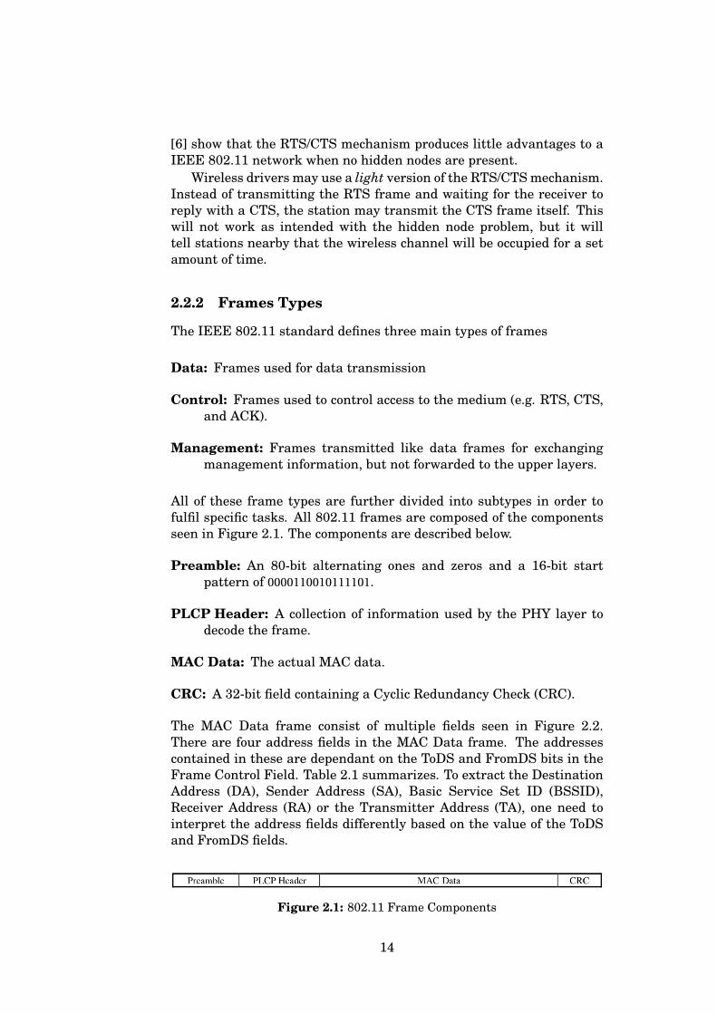
All of these frame types are further divided into subtypes in order tofulfil specific tasks. All 802.11 frames are composed of the componentsseen in Figure 2.1. The components are described below.

Preamble: An 80-bit alternating ones and zeros and a 16-bit startpattern of 0000110010111101.

PLCP Header: A collection of information used by the PHY layer todecode the frame.

MAC Data: The actual MAC data.

CRC: A 32-bit field containing a Cyclic Redundancy Check (CRC).

The MAC Data frame consist of multiple fields seen in Figure 2.2.There are four address fields in the MAC Data frame. The addressescontained in these are dependant on the ToDS and FromDS bits in theFrame Control Field. Table 2.1 summarizes. To extract the DestinationAddress (DA), Sender Address (SA), Basic Service Set ID (BSSID),Receiver Address (RA) or the Transmitter Address (TA), one need tointerpret the address fields differently based on the value of the ToDSand FromDS fields.

Figure 2.1: 802.11 Frame Components

14

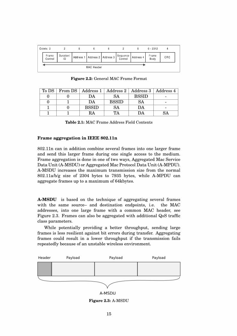
Figure 2.2: General MAC Frame Format

To DS From DS Address 1 Address 2 Address 3 Address 40 0 DA SA BSSID -0 1 DA BSSID SA -1 0 BSSID SA DA -1 1 RA TA DA SA

Table 2.1: MAC Frame Address Field Contents

Frame aggregation in IEEE 802.11n

802.11n can in addition combine several frames into one larger frameand send this larger frame during one single access to the medium.Frame aggregation is done in one of two ways, Aggregated Mac ServiceData Unit (A-MSDU) or Aggregated Mac Protocol Data Unit (A-MPDU).A-MSDU increases the maximum transmission size from the normal802.11a/b/g size of 2304 bytes to 7935 bytes, while A-MPDU canaggregate frames up to a maximum of 64kbytes.

A-MSDU is based on the technique of aggregating several frameswith the same source– and destination endpoints, i.e. the MACaddresses, into one large frame with a common MAC header, seeFigure 2.3. Frames can also be aggregated with additional QoS trafficclass parameters.

While potentially providing a better throughput, sending largeframes is less resilient against bit errors during transfer. Aggregatingframes could result in a lower throughput if the transmission failsrepeatedly because of an unstable wireless environment.

Figure 2.3: A-MSDU

15

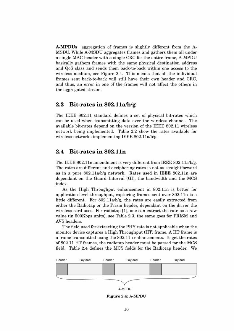
A-MPDUs aggregation of frames is slightly different from the A-MSDU. While A-MSDU aggregates frames and gathers them all undera single MAC header with a single CRC for the entire frame, A-MPDUbasically gathers frames with the same physical destination addressand QoS class and sends them back-to-back within one access to thewireless medium, see Figure 2.4. This means that all the individualframes sent back-to-back will still have their own header and CRC,and thus, an error in one of the frames will not affect the others inthe aggregated stream.

2.3 Bit-rates in 802.11a/b/g

The IEEE 802.11 standard defines a set of physical bit-rates whichcan be used when transmitting data over the wireless channel. Theavailable bit-rates depend on the version of the IEEE 802.11 wirelessnetwork being implemented. Table 2.2 show the rates available forwireless networks implementing IEEE 802.11a/b/g.

2.4 Bit-rates in 802.11n

The IEEE 802.11n amendment is very different from IEEE 802.11a/b/g.The rates are different and deciphering rates is not as straightforwardas in a pure 802.11a/b/g network. Rates used in IEEE 802.11n aredependant on the Guard Interval (GI), the bandwidth and the MCSindex.

As the High Throughput enhancement in 802.11n is better forapplication-level throughput, capturing frames sent over 802.11n is alittle different. For 802.11a/b/g, the rates are easily extracted fromeither the Radiotap or the Prism header, dependant on the driver thewireless card uses. For radiotap [1], one can extract the rate as a rawvalue (in 500Kbps units), see Table 2.3, the same goes for PRISM andAVS headers.

The field used for extracting the PHY rate is not applicable when themonitor device captures a High Throughput (HT) frame. A HT frame isa frame transmitted using the 802.11n enhancements. To get the ratesof 802.11 HT frames, the radiotap header must be parsed for the MCSfield. Table 2.4 defines the MCS fields for the Radiotap header. We

Figure 2.4: A-MPDU

16

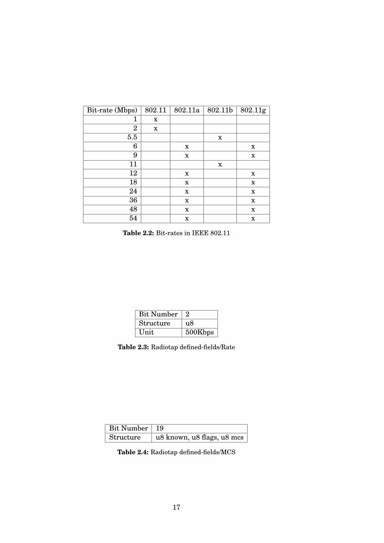
Bit-rate (Mbps) 802.11 802.11a 802.11b 802.11g1 x2 x

5.5 x6 x x9 x x

11 x12 x x18 x x24 x x36 x x48 x x54 x x

Table 2.2: Bit-rates in IEEE 802.11

Bit Number 2Structure u8Unit 500Kbps

Table 2.3: Radiotap defined-fields/Rate

Bit Number 19Structure u8 known, u8 flags, u8 mcs

Table 2.4: Radiotap defined-fields/MCS

17

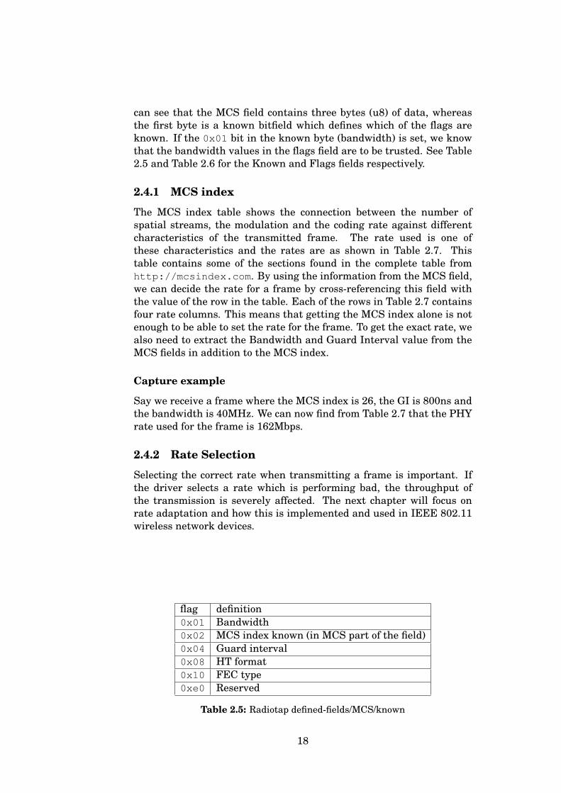
can see that the MCS field contains three bytes (u8) of data, whereasthe first byte is a known bitfield which defines which of the flags areknown. If the 0x01 bit in the known byte (bandwidth) is set, we knowthat the bandwidth values in the flags field are to be trusted. See Table2.5 and Table 2.6 for the Known and Flags fields respectively.

2.4.1 MCS index

The MCS index table shows the connection between the number ofspatial streams, the modulation and the coding rate against differentcharacteristics of the transmitted frame. The rate used is one ofthese characteristics and the rates are as shown in Table 2.7. Thistable contains some of the sections found in the complete table fromhttp://mcsindex.com. By using the information from the MCS field,we can decide the rate for a frame by cross-referencing this field withthe value of the row in the table. Each of the rows in Table 2.7 containsfour rate columns. This means that getting the MCS index alone is notenough to be able to set the rate for the frame. To get the exact rate, wealso need to extract the Bandwidth and Guard Interval value from theMCS fields in addition to the MCS index.

Capture example

Say we receive a frame where the MCS index is 26, the GI is 800ns andthe bandwidth is 40MHz. We can now find from Table 2.7 that the PHYrate used for the frame is 162Mbps.

2.4.2 Rate Selection

Selecting the correct rate when transmitting a frame is important. Ifthe driver selects a rate which is performing bad, the throughput ofthe transmission is severely affected. The next chapter will focus onrate adaptation and how this is implemented and used in IEEE 802.11wireless network devices.

flag definition0x01 Bandwidth0x02 MCS index known (in MCS part of the field)0x04 Guard interval0x08 HT format0x10 FEC type0xe0 Reserved

Table 2.5: Radiotap defined-fields/MCS/known

18

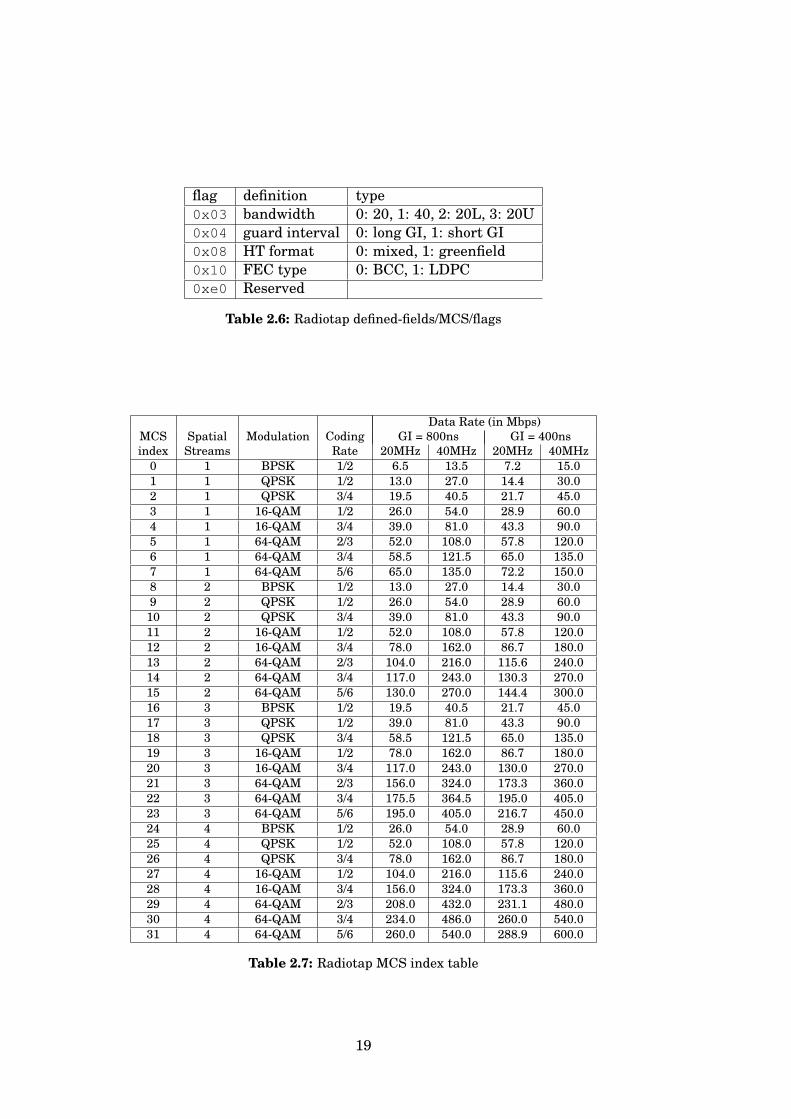
flag definition type0x03 bandwidth 0: 20, 1: 40, 2: 20L, 3: 20U0x04 guard interval 0: long GI, 1: short GI0x08 HT format 0: mixed, 1: greenfield0x10 FEC type 0: BCC, 1: LDPC0xe0 Reserved

Table 2.6: Radiotap defined-fields/MCS/flags

MCS Spatial Modulation CodingData Rate (in Mbps)

index Streams RateGI = 800ns GI = 400ns

20MHz 40MHz 20MHz 40MHz0 1 BPSK 1/2 6.5 13.5 7.2 15.01 1 QPSK 1/2 13.0 27.0 14.4 30.02 1 QPSK 3/4 19.5 40.5 21.7 45.03 1 16-QAM 1/2 26.0 54.0 28.9 60.04 1 16-QAM 3/4 39.0 81.0 43.3 90.05 1 64-QAM 2/3 52.0 108.0 57.8 120.06 1 64-QAM 3/4 58.5 121.5 65.0 135.07 1 64-QAM 5/6 65.0 135.0 72.2 150.08 2 BPSK 1/2 13.0 27.0 14.4 30.09 2 QPSK 1/2 26.0 54.0 28.9 60.0

10 2 QPSK 3/4 39.0 81.0 43.3 90.011 2 16-QAM 1/2 52.0 108.0 57.8 120.012 2 16-QAM 3/4 78.0 162.0 86.7 180.013 2 64-QAM 2/3 104.0 216.0 115.6 240.014 2 64-QAM 3/4 117.0 243.0 130.3 270.015 2 64-QAM 5/6 130.0 270.0 144.4 300.016 3 BPSK 1/2 19.5 40.5 21.7 45.017 3 QPSK 1/2 39.0 81.0 43.3 90.018 3 QPSK 3/4 58.5 121.5 65.0 135.019 3 16-QAM 1/2 78.0 162.0 86.7 180.020 3 16-QAM 3/4 117.0 243.0 130.0 270.021 3 64-QAM 2/3 156.0 324.0 173.3 360.022 3 64-QAM 3/4 175.5 364.5 195.0 405.023 3 64-QAM 5/6 195.0 405.0 216.7 450.024 4 BPSK 1/2 26.0 54.0 28.9 60.025 4 QPSK 1/2 52.0 108.0 57.8 120.026 4 QPSK 3/4 78.0 162.0 86.7 180.027 4 16-QAM 1/2 104.0 216.0 115.6 240.028 4 16-QAM 3/4 156.0 324.0 173.3 360.029 4 64-QAM 2/3 208.0 432.0 231.1 480.030 4 64-QAM 3/4 234.0 486.0 260.0 540.031 4 64-QAM 5/6 260.0 540.0 288.9 600.0

Table 2.7: Radiotap MCS index table

19

Chapter 3

Rate Adaptation

Rate Adaptation Algorithm (RAA), Rate Control Algorithm (RCA) orRate Selection Algorithm (RSA) (hereafter RAA), are algorithms andcontrol mechanisms located in either the driver of a 802.11 wirelessnetwork card, or implemented partly or fully in its hardware. Thepurpose of the RAA is to try to optimize the data throughput, orin some cases optimize the power consumption or other metrics ofa wireless device. The RAA consists of a set of rules on how toselect the preferred bit-rate for outgoing transmissions in a wirelessnetwork taking the condition of the channel into account. The conditionof a wireless channel can be determined by the level of the Signal-To-Noise Ratio (SNR), when classifying the condition based on thephysical characteristics of the channel, or it can be determined usingLink-Layer information such as packet-loss and retransmission ofoutgoing or incoming frames. Rate Adaptation Algorithms can use thephysical layer, the link layer, or even both to determine the state ofthe channel before scheduling an outgoing packet. This section willdescribe the different Rate Adaptation Algorithms used in this thesis,and the difference between them to be able to differentiate one fromanother. We will start by describing algorithms using the physicallayer in Section 2.1, then describe link-layer algorithms in Section 2.2.Thereafter we will describe algorithms using both the physical layerand the link-layer to determine the state of the wireless channel.

3.1 PHY-based algorithms

PHY-based rate adaptation algorithms, are algorithms using informa-tion about the physical condition of a wireless channel to determine thebest suited transmission rate for an outgoing frame. The hardware ofan 802.11 enabled wireless network device usually exports the currentsignal-to-noise ratio of the associated wireless channel. This can be usedin wireless drivers to determine the state of the channel by comparingthe SNR to a table of pre-calculated values between the SNR and trans-mission rates used by the channel.

21

3.1.1 Receiver-Based AutoRate (RBAR)

Receiver-Based AutoRate (RBAR) is a receiver based algorithm whichhas the goal of optimizing the application level throughput. While thisalgorithm is an important tool for theoretical comparison between otherRAAs, it cannot be implemented in current 802.11 networks because itrequires incompatible changes to the protocol. RBAR interprets someMAC control frames differently, and each data frame must include anew header field.

RBAR is an algorithm which works in the receiver end of twodata-exchanging parties over the 802.11 Wireless Local Area Network(WLAN) protocol. It uses RTS/CTS and the sender states at which datarate it wants to send the data packet. The only thing the receiverare allowed to suggest to the sender in the returning CTS packetis an alternate power level of the transmission. The data rate ofthe sender can be adjusted by Acknowledgement (ACK) or NegativeAcknowledgement (NACK) received from the receiver at the end of adata transmission.

To summarize, the protocol works like this:

1. The sender sends a RTS packet to the receiver

2. The receiver, if available, responds with a CTS packet, which mayor may not contain a suggestion to alter the transmit power of thedata transmission.

• If the CTS packet contains a message about changing thetransmit power, the sender may adjust the power accordingly

3. The sender starts sending the packet once it has received andinterpreted the CTS packet,

4. The receiver can adjust the rate of the next data transmission bysending ACK or NACK after the data transmission is completed.

• If changes to the data rate are suggested by the receiver,these changes are then used for the subsequent packettransmission.

The RBAR algorithm suffers from several issues [18], the main issuebeing that it is incompatible with the IEEE 802.11 standard, and assuch, cannot be deployed in any existing 802.11 wireless environments.

3.2 Link-Layer-Based algorithms

The link-layer in 802.11 WLAN protocol is used by some RAAs toestimate the quality of the channel. In the Link-Layer, one may collectinformation from data– or signalling frames, or both.

When using the data frame, there are two methods of finding thebest rate estimation for a channel. One may probe the channel, by

22

occasionally sending data frames at a rate different than the currentrate, or use the method of non-probing which never sends out probeframes.

3.2.1 Automatic Rate Fallback (ARF)

Automatic Rate Fallback [16], also called ARF, was the first RAA tobe published. The algorithm is a transmitter based rate adaptationalgorithm whose goal it is to increase the application level throughputof the wireless transmission. The idea behind ARF is that eachsender tries to use a higher transmission rate after a set number ofsuccessful transmissions at the current rate. If it experiences one ortwo consecutive losses, it falls back to the next lower rate. When ARFincreases the sending rate, the subsequent transmission decides if ARFwill continue to use the higher rate or fall back to the previous lowerone. The first packet is often referred to as a probing packet.

The algorithm works as follows:

1. If ACKs for two consecutive data packets are not received by thesender

• Then, the sender drops the transmission rate to the nextlower rate and starts a timer

2. If ten (10) consecutive ACKs are received

• Then, the transmission rate is raised to the next higher datarate and the timer is cancelled

3. If the timer expires, the transmission rate is raised as before,but with a condition that if an ACK is not received with the firsttransmission (the probing transmission), the data rate is loweredagain and the timer is restarted.

There are two problems with the ARF algorithm as described in[18], and quickly summarized. The algorithm has problems when theconditions of the channel changes very quickly, as it cannot adaptrapidly enough to the changing environment, and the algorithm alwaystries to increase the transmission rate even when the channel conditionsare very stable, which in terms lowers the application throughput. Indefence of the algorithm, it was mainly designed to work in a 2-rateenvironment.

3.2.2 Adaptive ARF (AARF)

AARF [18] is an algorithm based on ARF with the goal of performingbetter in stable channel conditions. ARF tries to increase thetransmission rate after 10 consecutive successful transmissions. Thiswill lower application-level throughput in stable channel conditions

23

where the next higher rate always fails. AARF tries to optimize thisby using history of the channel, and increase the number of consecutivesuccessful transmissions if the channel is stable and works best with afixed transmissions rate.

AARF behaves more or less like ARF, but unlike ARF it increasesthe number of consecutive successful transmissions it needs before ittries to send a transmission at a higher rate than the current one.It does this by remembering the number of failed attempts to probethe channel at a higher rate, and each time the probe transmissionfails, the algorithm multiplies the number of consecutive successfultransmissions by two, up to a maximum of 50. If a packet fails twicewhile in the current transmission, it lowers the transmission rate onestep and resets the consecutive successful transmission counter to 10just like ARF.

3.2.3 Adaptive Multi-Rate Retry (AMRR)

AMRR is an algorithm based on ARF with an additional BinaryExponential Backoff (BEB) much like AARF. The Atheros AR 5212chipset exports a mechanism to drivers called Multi-Rate Retry (MRR).The MRR is a descriptor table sent to the hardware along with thedata to be transmitted. The descriptor table is populated with fourrates used when transmitting the frame. Each rate is accompaniedwith a count value stating the number of times each rate is attemptedsent. To get the BEB in AMRR, the values of the count fields in therate/transmission count are set to one, c0=1, c1=1, c2=1 and c3=1. Formore information on the MRR, see Chapter 4. The transmission ratesare chosen based on the current transmission rate and the minimumrate of the wireless medium used. R3 is always set to the minimumtransmission rate, while R1 and R2 are set to the two rates just belowR0. R0 is determined by the previous value of R0 and the transmissionresults for the elapsed period.

3.2.4 Onoe

Onoe is a credit based algorithm where the credit is determined by thefrequency of successful deliveries, erroneous deliveries and retransmis-sions accumulated during a fixed invocation period of 1000ms (1sec). Asthe credit is determined using a relative long period of time, it is lesssensitive to individual packet loss than ARF and AMRR.

Onoe keeps track of the number of successfully transmitted framesand the number of error frames. Onoe increases its credit when lessthan 10% of packets require retransmission at a particular rate. Thecredit is increased until it reaches a value of 10, at which point thealgorithm starts sending transmissions at the next available higherrate, and the credit is reset to 0. In the case where retransmissionsoccurred for more than 10% of the packets sent in the last period, Onoereduces the rate to the next lower rate and the process is restarted with

24

a credit value of 0. If a rate has been abandoned because of transmissionfailures, Onoe marks that rate as a failure rate, and will not attempt touse it again until 10 seconds have elapsed.

3.2.5 SampleRate

SampleRate is an algorithm presented in “Bit-rate Selection in WirelessNetworks” by John C. Bicket [23]. This algorithm aims to providethe highest possible application throughput by using statistics andsampling over rates which could provide a better throughput than thecurrent rate. The algorithm keeps track of previously transmittedframes in a table for each rate for each station. Each rate in thetable contains the number of attempted transmissions, the number ofsuccessive failed transmissions, the number of ACK’ed frames, the totaltransmission time, average transmission time and lossless transmissiontime. This helps the algorithm select the rate which gives the maximumthroughput even if this is not the highest rate available.

The algorithm uses sampling over rates which are not the currentbest rate to build statistics about other rates in order to determine thebest suited rate for a given “health” of the wireless channel. This is doneby sending a frame at a selected rate other than the current one at everyten transmissions. The selection chooses its rate based on the estimatedframe transmission time for a given rate, which is based on previoustransmissions. Rates which have four successive failed transmissionsare not sampled, and if no rate has an estimated transmission timelower than the current rate, SampleRate sends the frame using therate which has the lowest average transmission time. To calculatethe estimated transmission time for a selected rate, the algorithm usestransmission results from the last ten seconds.

3.2.6 Minstrel

Minstrel [24] is a bit-rate selection algorithm designed by the teambehind the madwifi driver. Minstrel was designed to maximize thethroughput of wireless communications implementing the IEEE 802.11standard. Minstrel has many similarities to SampleRate, but thealgorithm has two different primary metrics. While SampleRate selectsits best rate based on the transmission time of each frame, Minstrelselects its bit-rate based on which rate can reach maximum throughputtaking into account the expected number of retransmissions, based onstatistical history of the wireless channel.

Minstrel, like SampleRate, probes the wireless channel in order toget an overview of its “health”. Minstrel defines these probing packetsas “Lookaround” packets and spends a set amount of time probing bit-rates other than the current best. The bit-rates selected for the probingframes are selected more intelligently than in SampleRate. Minstrel,for example, does not sample rates that cannot possibly provide a betterthroughput than the current best.

25

The rate statistics of the channel are evaluated periodically. Min-strel uses EWMA in order to update historical statistics, and new re-sults (results from the just completed time period) are added to thestatistics of every evaluation event.

3.2.7 PID

PID Rate Control [25] is a RAA created for use in the mac80211 frame-work [19]. The PID Rate Control builds on a general control theo-retic feedback technique which consists of the Proportional, Integraland Derivative elements. The basic function of the PID controller isa feedback loop that controls the output based on the input of the previ-ous output state. The algorithm is controlled through a set of variables,each set to tune the output of the PID controller in order to achieve thebest possible results.

3.2.8 MiSer

MiSer [27] is an algorithm constructed with the goal of optimizing localpower consumption. This algorithm does an offline calculation of theoptimal power/rate pairs using a wireless channel model. At runtime,the algorithm uses the offline constructed table to find the optimaltransmission rate and power level for each transmission.

The work presented in [18] mentions problems with this algorithm.A quick summary is that the algorithm requires a priori knowledgeabout the channel and the environment of the wireless network.

3.3 MAC802.11 framework

The mac80211 framework [19] is a framework written to help devel-opers write drivers for SoftMAC wireless devices. SoftMAC wirelessdevices require a software part in order to function properly. The soft-ware is responsible for controlling the MAC Sublayer Management En-tity, and the mac80211 framework is there to provide a common API fordriver developers.

The mac80211 framework comes with three built-in RAAs, twoimplementing the Minstrel algorithm, Minstrel and Minstrel HT andthe other being a PID Rate Control implementation. These RAAs canbe used by drivers using the mac80211 framework in order to not haveto implement their own. Minstrel HT is an implementation of Minstrelsupporting High Throughput (802.11n) rates.

26

Part III

Rate Adaptation Classifier(RAC)

27

Chapter 4

Design

The goal of this thesis is to design and implement an application capableof helping to classify Rate Adaptation Algorithms used by 802.11wireless devices. We will analyse and research different rate adaptationalgorithms in open-source drivers to better understand their behaviourand to be able to recognize traffic governed by these algorithms. Thiswill enable us to reliably distinguish one RAA from another.

Up to this point, we have mentioned many different RAAs. Weare going to focus on RAAs which are used in current popular open-source WLAN drivers such as madwifi. The ath5k and the ath9k driveruse the mac80211 framework, which currently deploys three RAAs,Minstrel, Minstrel HT and PID. The madwifi driver has four, AMRR,Onoe, SampleRate and Minstrel.

We chose the approach of manually analysing and classifyingRAAs instead of fingerprinting algorithms based on a machine-learningtechnique, as used by the authors of [21]. This because we believe theSVM technique does not deliver enough details when trying to classifyRAAs. We want information about traffic patterns, sampling– andrate change frequency, RTS/CTS usage, retry rates and other metricsmaking us able to reliably differentiate between algorithms. Thisapproach, while being very precise, requires the user to have deepknowledge of different RAAs. We will provide the user with a method ofanalysing the output of the tool and draw the correct conclusion basedon this method.

This chapter contains the initial research and characteristics of thepreviously mentioned RAAs. The RAAs are explained in detail and thefocus will be on locating characteristics of the RAA that make it standout. This will be used by the method in order to map traffic patternsand behaviour to algorithms.

4.1 Fingerprinting Rate Adaptation Algorithms

In order to distinguish RAAs, we will analyse and find specificcharacteristics for each of the selected RAAs. We will determine howwe can use this in order to decide which RAA is producing which traffic

29

pattern. Following this will be a discussion of what to use and how touse it.

Different RAAs have different characteristics. Some change theirrate selection at a set time interval, while others change their rateselection based on the number of transmitted packets. RAAs handleframe retransmission differently and the ones using Multi-Retry Chain(MRR) populate the retry chain differently. RAAs select their best ratebased on the rate they decide to be the best performing rate. The metricsused to decide the best performing rate may differ.

IEEE 802.11 WLANs retransmit failed frames. Rates used duringretransmission can differ from the rate used in the original frame, butthe sequence number is kept the same. There are different ways ofhandling this, but wireless devices using Atheros chipsets can passa descriptor to the hardware containing the selected rates. Thisdescriptor is called the MRR. Different RAAs populate the retry chaindifferently, and capturing retransmissions enables us to analyse thisrate selection.

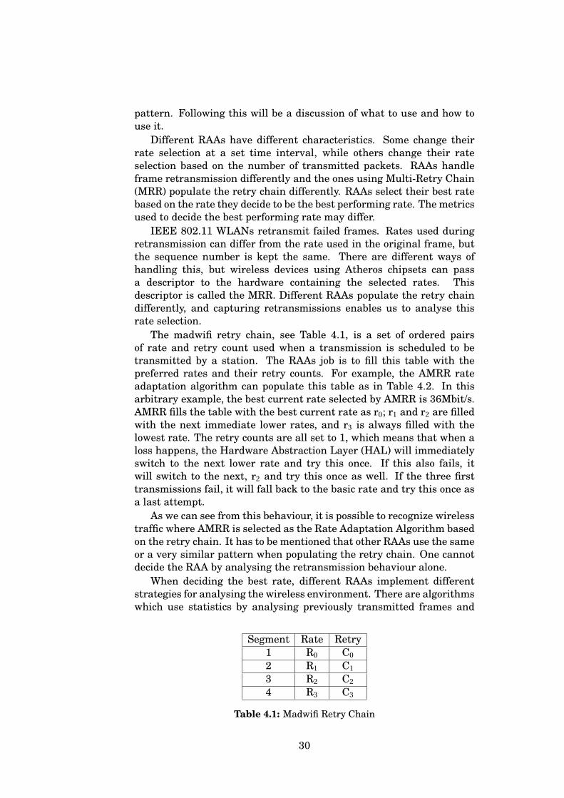
The madwifi retry chain, see Table 4.1, is a set of ordered pairsof rate and retry count used when a transmission is scheduled to betransmitted by a station. The RAAs job is to fill this table with thepreferred rates and their retry counts. For example, the AMRR rateadaptation algorithm can populate this table as in Table 4.2. In thisarbitrary example, the best current rate selected by AMRR is 36Mbit/s.AMRR fills the table with the best current rate as r0; r1 and r2 are filledwith the next immediate lower rates, and r3 is always filled with thelowest rate. The retry counts are all set to 1, which means that when aloss happens, the Hardware Abstraction Layer (HAL) will immediatelyswitch to the next lower rate and try this once. If this also fails, itwill switch to the next, r2 and try this once as well. If the three firsttransmissions fail, it will fall back to the basic rate and try this once asa last attempt.

As we can see from this behaviour, it is possible to recognize wirelesstraffic where AMRR is selected as the Rate Adaptation Algorithm basedon the retry chain. It has to be mentioned that other RAAs use the sameor a very similar pattern when populating the retry chain. One cannotdecide the RAA by analysing the retransmission behaviour alone.

When deciding the best rate, different RAAs implement differentstrategies for analysing the wireless environment. There are algorithmswhich use statistics by analysing previously transmitted frames and

Segment Rate Retry1 R0 C0

2 R1 C1

3 R2 C2

4 R3 C3

Table 4.1: Madwifi Retry Chain

30

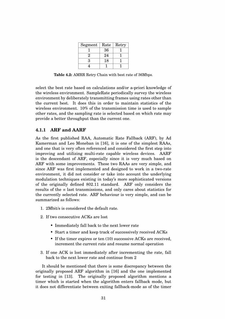
Segment Rate Retry1 36 12 24 13 18 14 1 1

Table 4.2: AMRR Retry Chain with best rate of 36Mbps.

select the best rate based on calculations and/or a-priori knowledge ofthe wireless environment. SampleRate periodically survey the wirelessenvironment by deliberately transmitting frames using rates other thanthe current best. It does this in order to maintain statistics of thewireless environment. 10% of the transmission time is used to sampleother rates, and the sampling rate is selected based on which rate mayprovide a better throughput than the current one.

4.1.1 ARF and AARF

As the first published RAA, Automatic Rate Fallback (ARF), by AdKamerman and Leo Moneban in [16], it is one of the simplest RAAs,and one that is very often referenced and considered the first step intoimproving and utilizing multi-rate capable wireless devices. AARFis the descendant of ARF, especially since it is very much based onARF with some improvements. These two RAAs are very simple, andsince ARF was first implemented and designed to work in a two-rateenvironment, it did not consider or take into account the underlyingmodulation techniques existing in today’s more sophisticated versionsof the originally defined 802.11 standard. ARF only considers theresults of the n last transmissions, and only cares about statistics forthe currently selected rate. ARF behaviour is very simple, and can besummarized as follows:

1. 2Mbit/s is considered the default rate.

2. If two consecutive ACKs are lost

• Immediately fall back to the next lower rate

• Start a timer and keep track of successively received ACKs

• If the timer expires or ten (10) successive ACKs are received,increment the current rate and resume normal operation

3. If one ACK is lost immediately after incrementing the rate, fallback to the next lower rate and continue from 2

It should be mentioned that there is some discrepancy between theoriginally proposed ARF algorithm in [16] and the one implementedfor testing in [13]. The originally proposed algorithm mentions atimer which is started when the algorithm enters fallback mode, butit does not differentiate between exiting fallback-mode as of the timer

31

expiring or when 10 successive ACKs are received. Either way, ARFexits fallback-mode and tries to send the next packet at the nexthigher rate. If no ACK is received for this first transmission, thealgorithm immediately falls back into fallback-mode and restarts thetimer. Reference [13] interprets the timer expiration and the 10successive ACKs as two distinctly different steps exiting fallback-mode;if 10 successive ACKs are received, the algorithm increases the rate tothe next higher rate and resumes normal operation. This requires theloss of two consecutive ACKs in order to fall back into fallback-mode.However, if the timer expires, ARF exits fallback-mode on the conditionthat the first transmission must be successfully ACK’d, if not it willimmediately fall back into fallback-mode.

AARF is very similar to ARF, although with some improvements,it still follows the same rules. The main difference between ARF andAARF is the way AARF handles stable network conditions. While ARFalways requires 10 successive ACKs to increase the rate, AARF hasthe ability to tweak this to some extent. AARF keeps incrementingthe number of successful ACKs required to increase the rate whenthe channel is in poor condition and the probing packet fails. Theprobing packet is the first packet sent after incrementing the currentrate. If this packet fails, AARF doubles the amount of successfullyacknowledged packets required in order to attempt another probepacket up to a maximum of 50 packets. This counter is reset to 10when the algorithm steps down to the next lower rate as a result oftwo consecutive lost ACKS.

Fingerprinting ARF/AARF

When fingerprinting ARF and AARF, a few characteristics are worthkeeping an eye on. One very important characteristic is that theycan only use the next higher rate after having successfully received 10consecutive ACKs for ARF, or 10, 20, 40 or 50 for AARF. Another is thatneither ARF nor AARF can change the current best rate by more thanone step at a time. For example, if the current best rate is 36Mbit/s,then ARF/AARF cannot switch to 12Mbit/s directly, it has to step downone rate at the time. This means that ARF/AARF will have to try 24–and 18– before it can try 12Mbit/s. To summarize, ARF/AARF havecharacteristics as shown below:

• Reducing the sendrate

– ARF/AARF reduce the current rate if two consecutive packetsare lost.

– They fall back to the next lower rate if probing packet fails.

• Frequency of best rate changes

– Current rate may change upwards as quickly as every 10packets.

32

– Current rate may change downwards as quickly as every 2packets.

– For AARF, the rate of change upwards may decrease as therequired consecutive successfully acknowledged packets maydouble up to a maximum of 50 packets before probing the nexthigher rate.

• Stepping

– Cannot skip rates while changing best rate.

4.1.2 Adaptive Multi-Rate Retry (AMRR)

The team behind AARF [18] realised that the Binary ExponentialBackoff mechanism used in AARF could still be useful when workingwith the Multi-Rate Retry capability exported by the hardware layer inAtheros based chipsets. The introduction of the BEB into the madwifidriver became AMRR. The madwifi driver was already using the MRRchain. The original madwifi driver periodically changed the MRRpopulation scheme (interval between 0.5 and 1 seconds), but the AMRRimplementation changed this in order to improve the algorithm reactiontime to short-term changes in the wireless environment.

Fingerprinting AMRR

When observing traffic governed by AMRR, we should easily be able todetect its characteristics. One is its inability to change the current bestby rate more than one step at the time. Unlike the more sophisticatedRAAs, which can change the current best rate from the highest to thelowest rate in one decision step, AMRR is only able to change thecurrent best rate to the immediate next lower or higher rate. AMRR,like its predecessors ARF and AARF, is fairly simple when it comesto how it decides whether or not to change the current rate. AMRRcollects statistics over a period of time to see if it needs to change thecurrent best rate. In the madwifi driver, this time period is set to1000ms (500ms if operating in station mode), which can be observedwhen looking at AMRR governed traffic.

Multi-Rate Retry

AMRRs Multi-Rate Retry Chain population is very simple. AMRR keepstrack of which rate is the current best rate, and puts this rate in theMRRs R0. As AMRR does not keep any other statistics of rates, itcannot determine if rates other than the immediate lower rates belowthe current best are better choices for the MRRs R1,2. R3 is alwayspopulated with the lowest base rate and all counters in MRR is set to1. The reason for setting the counters to 1 is to make AMRR moreresponsive to sudden changes in the wireless environment, althoughhaving the rate calculation run as seldom as it does, may defeat this

33

goal. A representation of AMRRs MRR population is shown in Table4.3.

This behaviour is very advantageous for our fingerprinting. Byobserving AMRR governed traffic, we should be able to see the contentsof the retry chain as packets are lost and retransmitted, and it shouldbe easy to recognize the pattern of AMRR.

• Multi-Rate Retry population

– Lowest baserate at R3.

– Retry fields are all always 1.

– R1,2 are always the two rates just below the current.


– Current rate changes only after rate update event (1000ms/500msfor madwifi).

– Can only change rates one step at a time.

4.1.3 Onoe

Onoe is the least known Rate Adaptation Algorithm in the madwifidriver. This algorithm is based on using credits for determining thebest rate. Rates collect credits by performing well during a samplingperiod, which is set to 1000ms in the madwifi driver. Every 1000ms,Onoe evaluates the result from the elapsed period and adjust creditsbased on a few simple rules as shown below:

• increase by one if less than 10% of the packets in the last intervalrequired a retransmission.

• decrease by one if more than 10% of the packets required aretransmission.

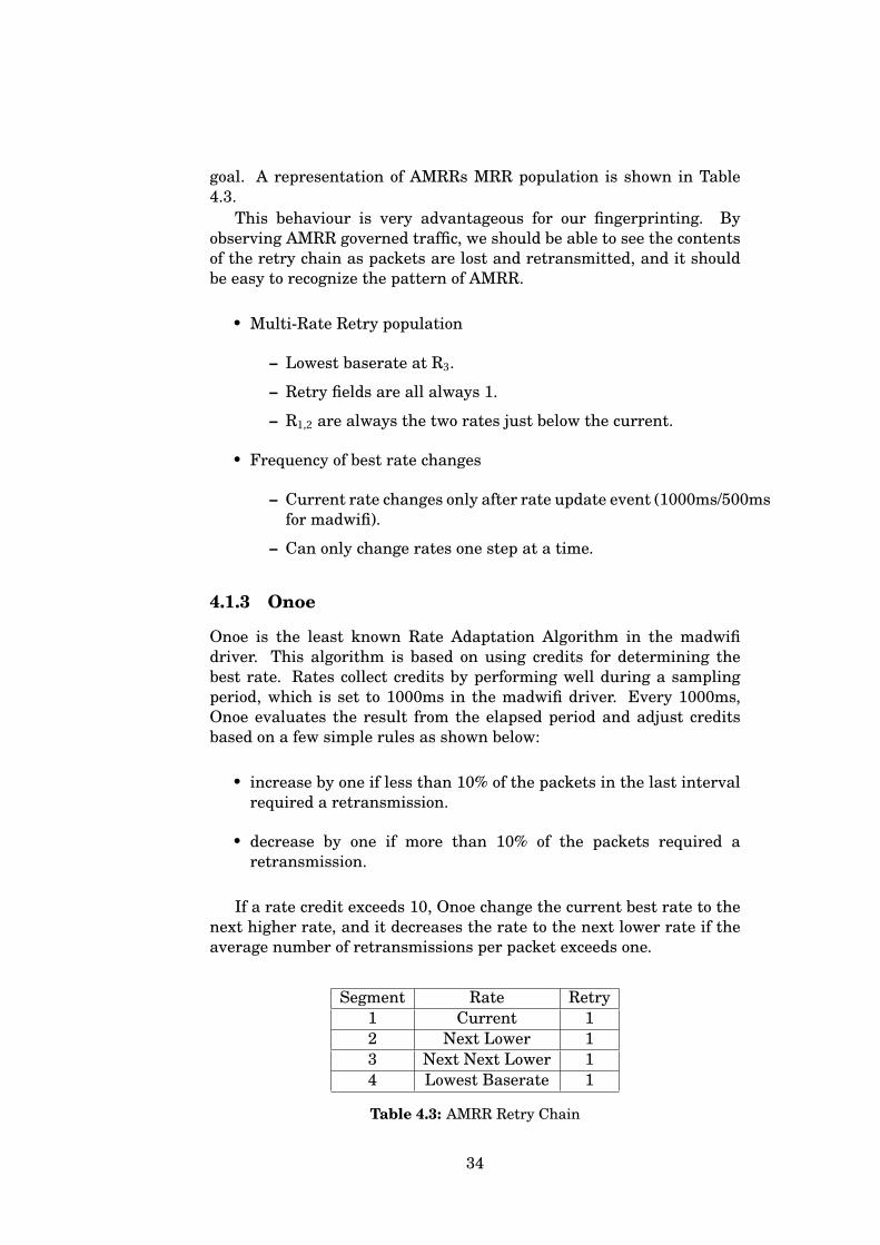
If a rate credit exceeds 10, Onoe change the current best rate to thenext higher rate, and it decreases the rate to the next lower rate if theaverage number of retransmissions per packet exceeds one.

Segment Rate Retry1 Current 12 Next Lower 13 Next Next Lower 14 Lowest Baserate 1

Table 4.3: AMRR Retry Chain

34

Multi-Rate Retry

Onoe populates the Multi-Rate Retry chain according to Table 4.4. TheMRR population for Onoe is very similar to ARF/AARF and AMRR. R0

is the current best rate and R1,2 contains the immediate lower rates. R3

is always the lowest base rate. The count fields for Onoe are populatedwith C0 = 4 and C1−3 = 2.

Fingerprinting Onoe

When trying to fingerprint Onoe, there are certain characteristics wecan look for. Mainly, we look at the MRR and how it is populated. Wealso know that Onoe has the ability to change the current best rate onlyevery 1000ms.


– Population as seen in Table 4.4.

• Best rate changes

– Frequency of rate changes.

– Can only change rates one step at a time.

4.1.4 SampleRate

SampleRate, first published by J. Bicket in [23] was the first RAA whichdid not take for granted that lower transmission rates would lead to alower chance of packet loss.

SampleRate aims to maximize the throughput on wireless linksby choosing the bit-rate which it predicts to have the smallest per-packet transmission time based on probing alternative bit-rates thanthe current rate and estimating the transmission time based on theresult of probe packets.

Fingerprinting SampleRate

In order to decide whether observed traffic from a wireless stationis using the SampleRate RAA, we need to analyse the behaviourof SampleRate, and try to find characteristics which are typical toSampleRate. This section will find and describe typical behaviour

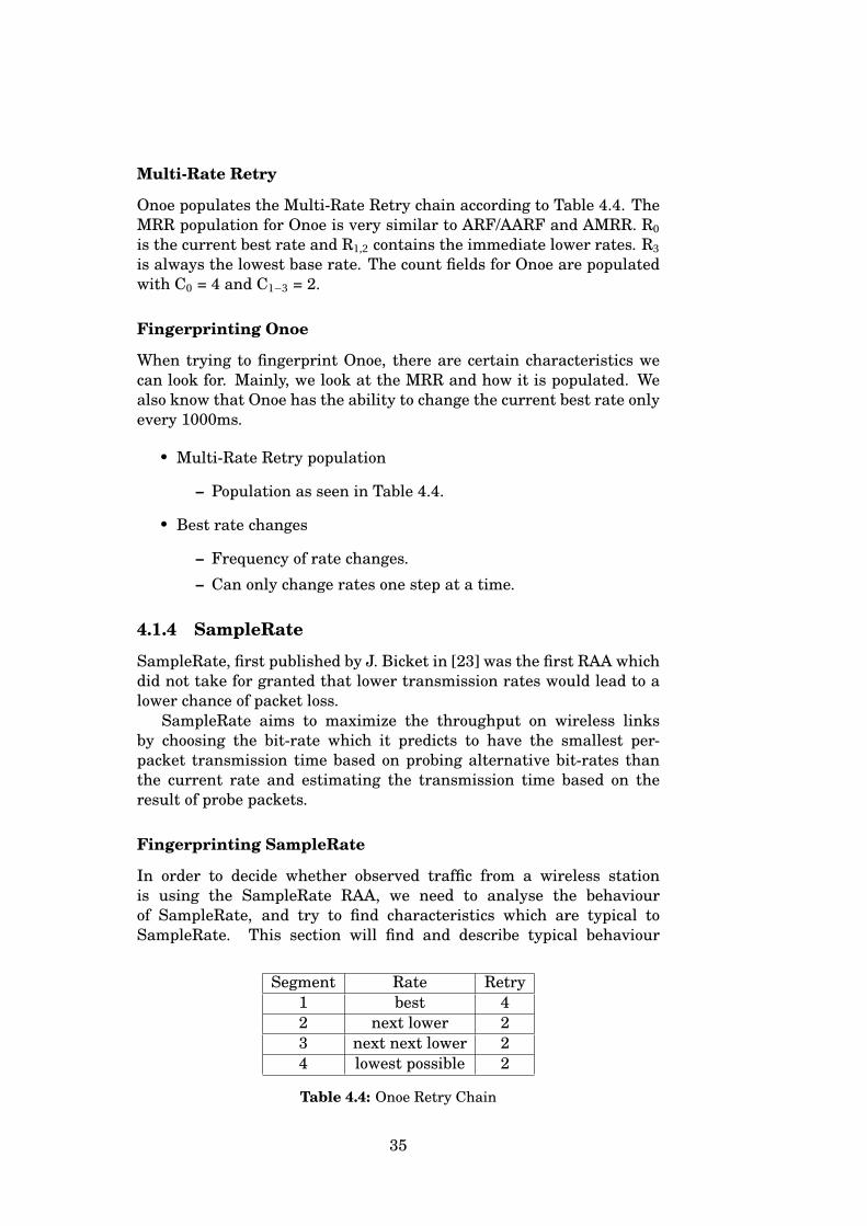
Segment Rate Retry1 best 42 next lower 23 next next lower 24 lowest possible 2

Table 4.4: Onoe Retry Chain

35

for SampleRate, and create a scheme of how we can determine thatobserved behaviour has originated from a station using SampleRate asits RAA.

New associations

The initial transmission when using SampleRate is set to the highestrate possible. For 802.11.b/g, this is 54Mbit/s. SampleRate will transmiteach packet four times before it considers a rate as not working. Ifwe were able to pick up the traffic at the initial stages of a connectionbetween a station and an access-point, we would see that the first packetis transmitted at 54Mbit/s.

Multi-Rate Retry Chain

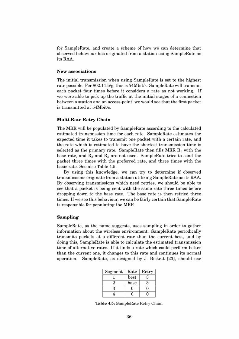
The MRR will be populated by SampleRate according to the calculatedestimated transmission time for each rate. SampleRate estimates theexpected time it takes to transmit one packet with a certain rate, andthe rate which is estimated to have the shortest transmission time isselected as the primary rate. SampleRate then fills MRR R1 with thebase rate, and R2 and R3 are not used. SampleRate tries to send thepacket three times with the preferred rate, and three times with thebasic rate. See also Table 4.5.

By using this knowledge, we can try to determine if observedtransmissions originate from a station utilizing SampleRate as its RAA.By observing transmissions which need retries, we should be able tosee that a packet is being sent with the same rate three times beforedropping down to the base rate. The base rate is then retried threetimes. If we see this behaviour, we can be fairly certain that SampleRateis responsible for populating the MRR.

Sampling

SampleRate, as the name suggests, uses sampling in order to gatherinformation about the wireless environment. SampleRate periodicallytransmits packets at a different rate than the current best, and bydoing this, SampleRate is able to calculate the estimated transmissiontime of alternative rates. If it finds a rate which could perform betterthan the current one, it changes to this rate and continues its normaloperation. SampleRate, as designed by J. Bickett [23], should use

Segment Rate Retry1 best 32 base 33 0 04 0 0

Table 4.5: SampleRate Retry Chain

36

10% of the transmission time for sampling other rates. The ratesare chosen intelligently, as SampleRate only samples rates which mayperform better than the current best and have not recently seen packetsunacknowledged four successive times. A rate is considered unusable iftransmissions using the rate fails four times in a row, and is then notconsidered for transmission or sampling for the next 10 seconds. Byselecting the sampling rates intelligently, SampleRate will not samplea rate which has a theoretical transmission time lower than the currentrate. For example, if the current rate is 11Mbit/s on a 802.11b network,and the average transmission time of 11Mbit/s is less than the losslesstransmission time of 5.5Mbit/s which is 2976µs [23], SampleRate willnot select 5.5Mbit/s as a sampling rate. However, as SampleRatecontinues to transmit packets on 11Mbit/s, the wireless environmentmay degrade, and the average transmission time of 11Mbit/s mayincrease above 2976µs. At this point, 5.5Mbit/s is eligible for sampling.SampleRate will now chose 5.5Mbit/s as the sampling rate in order todetermine if it performs better than the current 11Mbit/s rate.

As SampleRate periodically samples rates other than the currentone (if there exist a better alternative), we could possibly use this toour advantage. By keeping track of the number of packets sent by astation, we could, e.g. observe every 10th packet, and look for changesin the rate selection. If we see that the rate selected is different fromthe current (the last n packets), we could consider this as a samplingpacket and continue to observe traffic with this in mind. If we see thatthis trend continues, we could conclude that the observed traffic may becontrolled by SampleRate.

Quarantine

As mentioned, sample rate has the ability to “quarantine” a ratewhen it suffers from four successive failures. When a rate has beenquarantined, it will not be eligible for transmission or sampling duringthe next ten seconds. This can be used by keeping track of each ratewhich has been observed, and setting a timestamp when the rate waslast used. If we observe a rate failing four successive times, and do notsee this rate being used for the next ten seconds, it might be SampleRatewhich dictates the rate selection for the station in question.

Size buckets

The madwifi implementation of SampleRate additionally uses bucketsto separate three packet sizes. The driver separates transmissions intopackets with a size from 0– up to 250bytes, packets with size from250– to 1600bytes and the packets from 1600– to 3000bytes, see Table4.6. This means that SampleRate handles transmissions differently fordifferent size packets. Packets of size smaller than 250bytes may havea different best rate than packets with a size of 1500bytes. This is anadvantage for us. By implementing tests which looks at transmissions

37

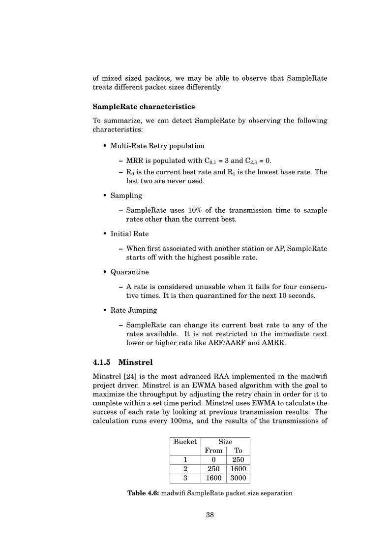
of mixed sized packets, we may be able to observe that SampleRatetreats different packet sizes differently.

SampleRate characteristics

To summarize, we can detect SampleRate by observing the followingcharacteristics:


– MRR is populated with C0,1 = 3 and C2,3 = 0.– R0 is the current best rate and R1 is the lowest base rate. The

last two are never used.

• Sampling

– SampleRate uses 10% of the transmission time to samplerates other than the current best.

• Initial Rate

– When first associated with another station or AP, SampleRatestarts off with the highest possible rate.

• Quarantine

– A rate is considered unusable when it fails for four consecu-tive times. It is then quarantined for the next 10 seconds.

• Rate Jumping

– SampleRate can change its current best rate to any of therates available. It is not restricted to the immediate nextlower or higher rate like ARF/AARF and AMRR.

4.1.5 Minstrel

Minstrel [24] is the most advanced RAA implemented in the madwifiproject driver. Minstrel is an EWMA based algorithm with the goal tomaximize the throughput by adjusting the retry chain in order for it tocomplete within a set time period. Minstrel uses EWMA to calculate thesuccess of each rate by looking at previous transmission results. Thecalculation runs every 100ms, and the results of the transmissions of

Bucket SizeFrom To

1 0 2502 250 16003 1600 3000

Table 4.6: madwifi SampleRate packet size separation

38

the last 100ms are given a 25% weight in the EWMA calculation. Thisparameter of 25% can be set in the driver by a programmer.

Fingerprinting Minstrel

Minstrels behaviour is somewhat similar to SampleRates. Thereare a few differences, and these are what we want to find, as wellas determine how to use these differences to be able to fingerprintMinstrel.

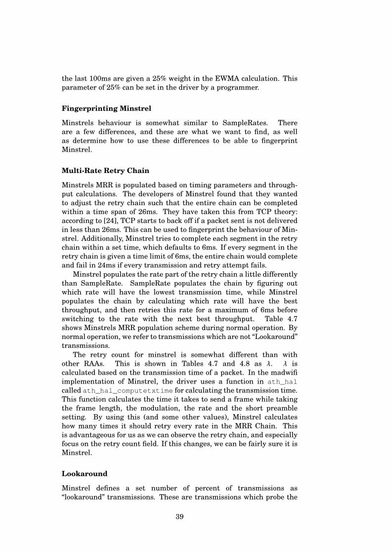
Multi-Rate Retry Chain

Minstrels MRR is populated based on timing parameters and through-put calculations. The developers of Minstrel found that they wantedto adjust the retry chain such that the entire chain can be completedwithin a time span of 26ms. They have taken this from TCP theory:according to [24], TCP starts to back off if a packet sent is not deliveredin less than 26ms. This can be used to fingerprint the behaviour of Min-strel. Additionally, Minstrel tries to complete each segment in the retrychain within a set time, which defaults to 6ms. If every segment in theretry chain is given a time limit of 6ms, the entire chain would completeand fail in 24ms if every transmission and retry attempt fails.

Minstrel populates the rate part of the retry chain a little differentlythan SampleRate. SampleRate populates the chain by figuring outwhich rate will have the lowest transmission time, while Minstrelpopulates the chain by calculating which rate will have the bestthroughput, and then retries this rate for a maximum of 6ms beforeswitching to the rate with the next best throughput. Table 4.7shows Minstrels MRR population scheme during normal operation. Bynormal operation, we refer to transmissions which are not “Lookaround”transmissions.

The retry count for minstrel is somewhat different than withother RAAs. This is shown in Tables 4.7 and 4.8 as λ. λ iscalculated based on the transmission time of a packet. In the madwifiimplementation of Minstrel, the driver uses a function in ath_halcalled ath_hal_computetxtime for calculating the transmission time.This function calculates the time it takes to send a frame while takingthe frame length, the modulation, the rate and the short preamblesetting. By using this (and some other values), Minstrel calculateshow many times it should retry every rate in the MRR Chain. Thisis advantageous for us as we can observe the retry chain, and especiallyfocus on the retry count field. If this changes, we can be fairly sure it isMinstrel.

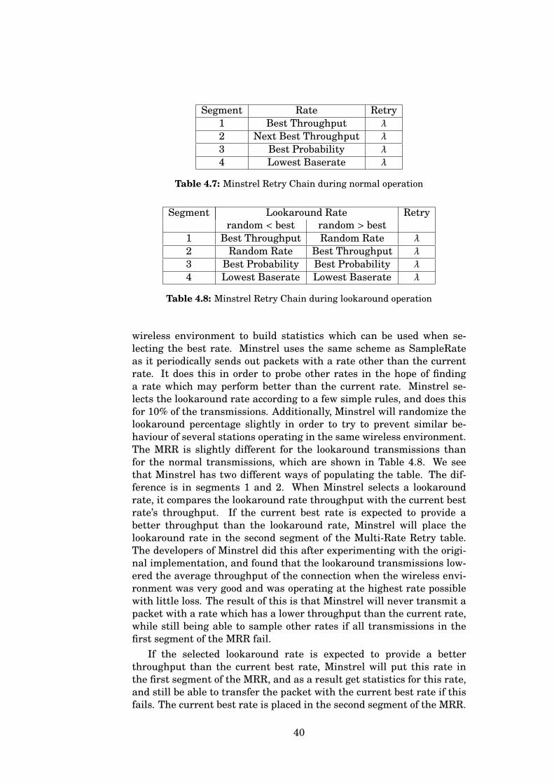
Lookaround

Minstrel defines a set number of percent of transmissions as“lookaround” transmissions. These are transmissions which probe the

39

Segment Rate Retry1 Best Throughput λ

2 Next Best Throughput λ

3 Best Probability λ

4 Lowest Baserate λ

Table 4.7: Minstrel Retry Chain during normal operation

Segment Lookaround Rate Retryrandom < best random > best

1 Best Throughput Random Rate λ

2 Random Rate Best Throughput λ

3 Best Probability Best Probability λ

4 Lowest Baserate Lowest Baserate λ

Table 4.8: Minstrel Retry Chain during lookaround operation

wireless environment to build statistics which can be used when se-lecting the best rate. Minstrel uses the same scheme as SampleRateas it periodically sends out packets with a rate other than the currentrate. It does this in order to probe other rates in the hope of findinga rate which may perform better than the current rate. Minstrel se-lects the lookaround rate according to a few simple rules, and does thisfor 10% of the transmissions. Additionally, Minstrel will randomize thelookaround percentage slightly in order to try to prevent similar be-haviour of several stations operating in the same wireless environment.The MRR is slightly different for the lookaround transmissions thanfor the normal transmissions, which are shown in Table 4.8. We seethat Minstrel has two different ways of populating the table. The dif-ference is in segments 1 and 2. When Minstrel selects a lookaroundrate, it compares the lookaround rate throughput with the current bestrate’s throughput. If the current best rate is expected to provide abetter throughput than the lookaround rate, Minstrel will place thelookaround rate in the second segment of the Multi-Rate Retry table.The developers of Minstrel did this after experimenting with the origi-nal implementation, and found that the lookaround transmissions low-ered the average throughput of the connection when the wireless envi-ronment was very good and was operating at the highest rate possiblewith little loss. The result of this is that Minstrel will never transmit apacket with a rate which has a lower throughput than the current rate,while still being able to sample other rates if all transmissions in thefirst segment of the MRR fail.

If the selected lookaround rate is expected to provide a betterthroughput than the current best rate, Minstrel will put this rate inthe first segment of the MRR, and as a result get statistics for this rate,and still be able to transfer the packet with the current best rate if thisfails. The current best rate is placed in the second segment of the MRR.

40

Exponential Weighted Moving Average (EWMA)

Minstrel calculates the EWMA periodically, and defaults to every100ms. This means that the current best rate cannot be changed moreoften than every 100ms. This can be used in our fingerprinting whenlistening to transmissions from a station.. We can find the current bestby looking at normal transmissions and observe how often this changes.If this time is about 100ms, it could be that we are observing trafficgoverned by Minstrel.

Minstrel characteristics

To summarize, we can detect Minstrel by observing the followingcharacteristics:


– Lowest baserate at R3.

– Changing count for the retry fields (C0−3).

– Not necessarily decreasing rates from R0−3. This means thatretransmissions may be transmitted at a higher rate than theoriginal rate.

• Lookaround

– Every 10th packet (with some randomness) is a lookaroundpacket.

– Rarely see lookaround packets when operating at the highestrate with minimal loss.


– Best rate changes at most every 100ms.

• Rate jumping

– Best rate may change by more than one step, just likeSampleRate.

4.1.6 PID

The PID rate control [25] is one of the RAAs implemented inthe mac80211 framework. The PID RAA is based on the Propor-tional–Integral–Derivative controller , next to Minstrel1. The purposeof the PID controller is to provide a mechanism for calculating andadjusting the output based on three input parameters. The PID Con-trollers Proportional control decides the initial behaviour of the output.This may start slow or fast dependant on the desired outcome. The PIDControllers Integral control is responsible for adjustments over time,

1PID Controller: http://en.wikipedia.org/wiki/PID_controller

41

and the Derivative control is in charge of trying to even out the adjust-ment in order for the output to converge to a desired state. The valuesof these three controls, the Proportional Coefficient (CP), the IntegralCoefficient (CI) and Derivative Coefficient (CD), are adjusted carefullyin order to achieve the desired output.

The PID RAA utilizes the Proportional–Integral–Derivative (PID)Controllers mechanism by implementing the following equation whichcalculates an adjustment value which is used to decide the transmissionrate for the next packet (Equation 4.1):

ad j =CP ·er r +CI ·er r _av g +CD · (er r − l ast_er r ) · (1+ shar peni ng ) (4.1)

adjadjustment value that is used to switch TX rate (see below)

errcurrent error: target vs. current failed frames percentage

last_errlast error

err_avgaverage (i.e. “poor man’s integral”) of recent errors

sharpeningnon-zero when fast response is needed (i.e. right after associationor no frames sent for a long time), approaching zero over time

CPProportional coefficient

CIIntegral coefficient

CDDerivative coefficient

CP, CI and CD are determined during compile time of the frameworkand are set to 15, 9 and 15 respectively. After the calculation, PID triesto find a better rate using the adjustment value looking for a rate whichhas not shown a worse error rate than the current one.

The PID RAA does not continuously update its current bestrate. Like the many other RAA mechanisms, it adjusts its bestrate periodically. The mac80211 framework’s implementation of thealgorithm has this period set to 125ms. Although it is not certain thatit runs the update every 125ms (less updates may happen if no packetshas been sent during a period longer than the 125ms period), with areasonable amount of traffic, the adjustment may occur as often as every125ms.

42

Fingerprinting PID

To be able to recognize traffic governed by PID, there are a fewcharacteristics we could try to observe. Like SampleRate and Minstrel,PID is not restricted to changing to the immediate next higher or lowerrate. PID may change the current best rate to any rate amongst theavailable rates as it sees fit. We could also try to track the frequency ofbest-rate changes. If the current best rate does not change more oftenthan every 125ms, this could be an indication that the traffic is PID.

PID characteristics

To summarize, PID has the following characteristics:


– Best rate changes at most every 125ms, but the upper limitmay vary.

• Rate jumping

– Best rate may change to any available rate.

4.2 Retry Strategies

Different drivers and RAAs implement different strategies for retrans-missions. A retransmission happens when the receiver either does notacknowledge, or sends a negative acknowledgement, for a transmittedframe. The sender can retransmit the frame at the same rate as theoriginal frame or select another. This section will list three retransmis-sion strategies.

4.2.1 Strategy A: Simple Fallback

This is the simplest of strategies. It basically tries all rates once until ithits its predetermined limit or reaches the base rate of 1Mbps. It thengives up and declares the packet as lost. Algorithms known to use thisstrategy are the madwifi implementations of AMRR and Onoe.

The madwifi implementations of AMRR and Onoe are described inSections 4.1.2 and 4.1.3.

4.2.2 Strategy B: Best-rate or Base-rate

This is a very simple strategy. It is implemented in the madwifi versionof the SampleRate RAA and uses two or three different rates whenretrying a transmission. The base rate is always the last attemptedrate. This strategy is recognizable by seeing the best-rate attempteda set number of times followed by a number of base-rate transmissionattempts. Variations of this strategy are seen in the implementation ofSampleRate in the madwifi driver where there can be three differentrates when retransmissions occur while sampling the channel.

43

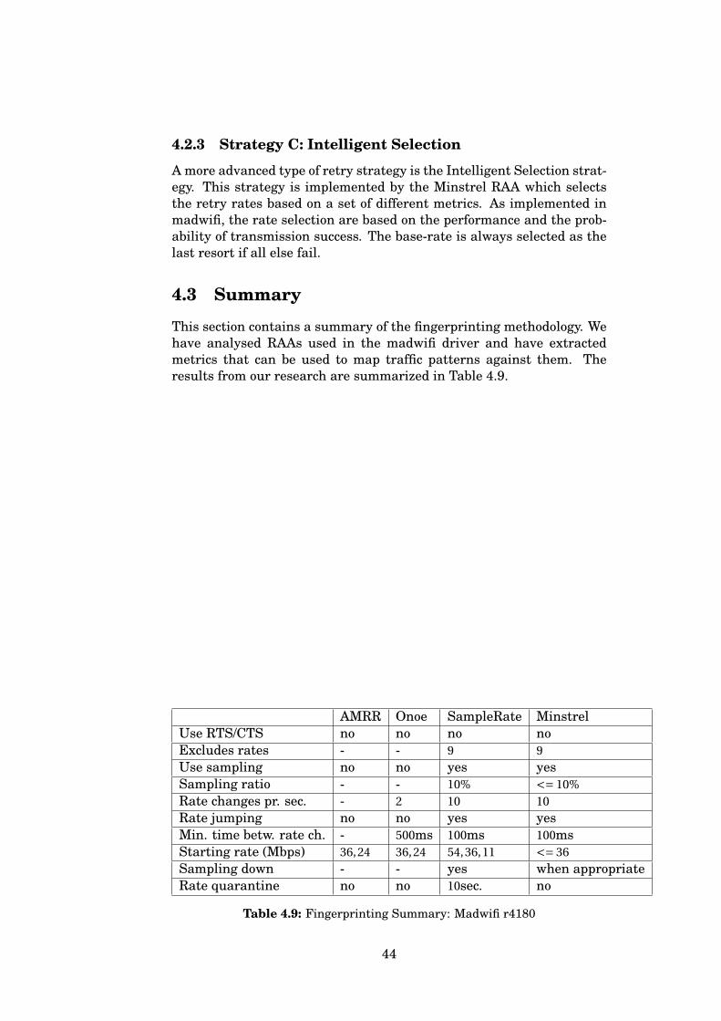
4.2.3 Strategy C: Intelligent Selection

A more advanced type of retry strategy is the Intelligent Selection strat-egy. This strategy is implemented by the Minstrel RAA which selectsthe retry rates based on a set of different metrics. As implemented inmadwifi, the rate selection are based on the performance and the prob-ability of transmission success. The base-rate is always selected as thelast resort if all else fail.

4.3 Summary

This section contains a summary of the fingerprinting methodology. Wehave analysed RAAs used in the madwifi driver and have extractedmetrics that can be used to map traffic patterns against them. Theresults from our research are summarized in Table 4.9.

AMRR Onoe SampleRate MinstrelUse RTS/CTS no no no noExcludes rates - - 9 9Use sampling no no yes yesSampling ratio - - 10% <= 10%Rate changes pr. sec. - 2 10 10Rate jumping no no yes yesMin. time betw. rate ch. - 500ms 100ms 100msStarting rate (Mbps) 36,24 36,24 54,36,11 <= 36Sampling down - - yes when appropriateRate quarantine no no 10sec. no

Table 4.9: Fingerprinting Summary: Madwifi r4180

44

Chapter 5

Implementation

This chapter contains information about the Rate Adaptation Classifier(RAC). RAC is a small piece of software which aims to present the userwith useful information regarding wireless stations in the near vicinity.RAC uses a standard WLAN interface in monitor mode, and supportsthe usual 802.11a/b/g standards as well as the newer 802.11n.

This small piece of software is built using inspiration from anothertool aimed at analysing the behaviour of wireless networks, namelyhorst [14].

The RAC software is built on a number of different modules. Thesemodules are logical pieces handling different parts of the process ofcapturing and analysing the wireless traffic.

5.1 Packet Capture Engine

To be able to analyse packets that are transmitted over the air betweenan Access Point and a station, we need to configure the kernel to reportevery frame received by the wireless interface. This mode is calledpromiscuous mode and is enabled by either using exported functionsin one of several frameworks for packet capturing or by setting theinterface manually to promiscuous mode using a kernel syscall or anapplication such as ifconfig [2].

When capturing packets, there are several libraries one can use inorder to ease the process, or one can capture raw packets by manuallysetting the interface into promiscuous mode and reading packets fromit.

When capturing packets from a wireless interface, it is most likelypossible to capture packets prepended with either the Radiotap– [1],the Prism– or the AVS header format. These are headers whichallows the driver to add information to the packet in order for user-space applications to read different statistics and/or driver-relatedinformation before reading the actual packet content.

45

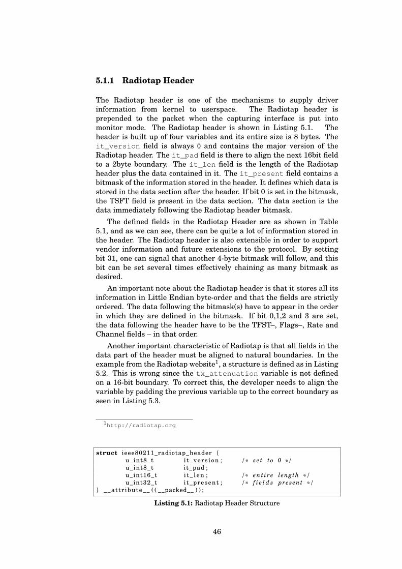
5.1.1 Radiotap Header

The Radiotap header is one of the mechanisms to supply driverinformation from kernel to userspace. The Radiotap header isprepended to the packet when the capturing interface is put intomonitor mode. The Radiotap header is shown in Listing 5.1. Theheader is built up of four variables and its entire size is 8 bytes. Theit_version field is always 0 and contains the major version of theRadiotap header. The it_pad field is there to align the next 16bit fieldto a 2byte boundary. The it_len field is the length of the Radiotapheader plus the data contained in it. The it_present field contains abitmask of the information stored in the header. It defines which data isstored in the data section after the header. If bit 0 is set in the bitmask,the TSFT field is present in the data section. The data section is thedata immediately following the Radiotap header bitmask.

The defined fields in the Radiotap Header are as shown in Table5.1, and as we can see, there can be quite a lot of information stored inthe header. The Radiotap header is also extensible in order to supportvendor information and future extensions to the protocol. By settingbit 31, one can signal that another 4-byte bitmask will follow, and thisbit can be set several times effectively chaining as many bitmask asdesired.

An important note about the Radiotap header is that it stores all itsinformation in Little Endian byte-order and that the fields are strictlyordered. The data following the bitmask(s) have to appear in the orderin which they are defined in the bitmask. If bit 0,1,2 and 3 are set,the data following the header have to be the TFST–, Flags–, Rate andChannel fields – in that order.

Another important characteristic of Radiotap is that all fields in thedata part of the header must be aligned to natural boundaries. In theexample from the Radiotap website1, a structure is defined as in Listing5.2. This is wrong since the tx_attenuation variable is not definedon a 16-bit boundary. To correct this, the developer needs to align thevariable by padding the previous variable up to the correct boundary asseen in Listing 5.3.

1http://radiotap.org

struct ieee80211_radiotap_header {u_int8_t i t_vers ion ; /* s e t to 0 */u_int8_t it_pad ;u_int16_t i t _ l en ; /* en t i r e length */u_int32_t i t_present ; /* f i e l d s present */

} __attr ibute__ ( ( __packed__ ) ) ;

Listing 5.1: Radiotap Header Structure

46

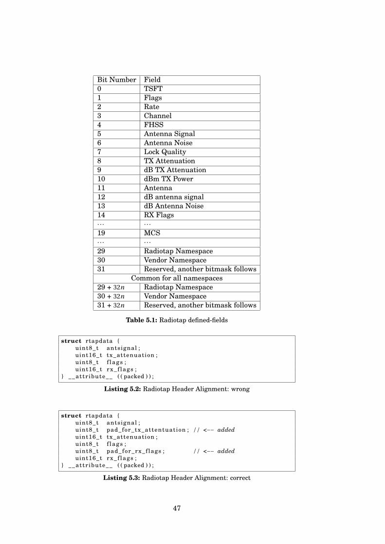
Bit Number Field0 TSFT1 Flags2 Rate3 Channel4 FHSS5 Antenna Signal6 Antenna Noise7 Lock Quality8 TX Attenuation9 dB TX Attenuation10 dBm TX Power11 Antenna12 dB antenna signal13 dB Antenna Noise14 RX Flags· · · · · ·19 MCS· · · · · ·29 Radiotap Namespace30 Vendor Namespace31 Reserved, another bitmask follows

Common for all namespaces29 + 32n Radiotap Namespace30 + 32n Vendor Namespace31 + 32n Reserved, another bitmask follows

Table 5.1: Radiotap defined-fields

struct rtapdata {uint8_t antsignal ;uint16_t tx_attenuation ;uint8_t f lags ;uint16_t rx_f lags ;

} __attr ibute__ ( ( packed ) ) ;

Listing 5.2: Radiotap Header Alignment: wrong

struct rtapdata {uint8_t antsignal ;uint8_t pad_for_tx_attentuation ; // <−− addeduint16_t tx_attenuation ;uint8_t f lags ;uint8_t pad_for_rx_f lags ; // <−− addeduint16_t rx_f lags ;

} __attr ibute__ ( ( packed ) ) ;

Listing 5.3: Radiotap Header Alignment: correct

47

5.1.2 PRISM Header

The PRISM header is a consistent 144 bytes long header which isprepended to the 802.11 WLAN header when a WLAN interface whosupports it is set to monitor mode. The PRISM header, as seen in Listing5.4, contains information about the physical characteristics of a receivedframe. The information contained within the header is amongst othersthe physical rate, which is very important for this work.

5.1.3 AVS Header

The AVS header was designed to replace the PRISM header format.The AVS header format extends the PRISM header by providing moreinformation about the capture when capturing 802.11a and 802.11gpackets.

5.1.4 Capturing RAW Packets

Capturing RAW packets from an interface is quite easy when workingwith most Linux WLAN drivers. As long as the driver supports Monitormode, one can capture all packets the interface is able to see.

By capturing RAW packets, the application needs to implement allthe logic surrounding the packet capture process. This means openingthe device, setting the device into promiscuous mode and controlling theread process.

5.1.5 Capture using PCAP

Linux libpcap [3] implements the Packet Capture (PCAP) API. Thelibpcap library hides much of the configuration and set-up process fromthe developer and provides a powerful api for controlling the networkinterface. Many popular applications use libpcap for capturing packets,e.g. Wireshark [4]. RAC is implemented using the PCAP library as itsupports the Radiotap extensions.

5.1.6 Parsing Radiotap Headers

Parsing radiotap headers is done using the Linux kernel radiotapparser. This parser provides a callback-like interface for extractinginformation from the radiotap header. RAC use this parser in orderto extract information like the PHY bit-rate from received frames.

5.1.7 Parsing 802.11 WLAN Frames

Parsing 802.11 WLAN frames is manually performed by RAC. RACcontains a rudimentary 802.11 WLAN header parser which onlyextracts the important bits. The extracted values are the packet length,frame type, the sender – and the destination address.

48

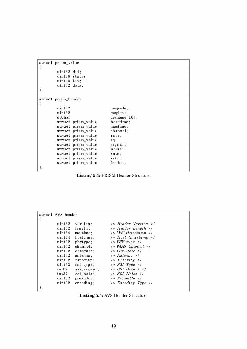
struct prism_value{

uint32 did ;uint16 status ;uint16 len ;uint32 data ;

} ;

struct prism_header{

uint32 msgcode ;uint32 msglen ;u8char devname [ 1 6 ] ;struct prism_value hosttime ;struct prism_value mactime ;struct prism_value channel ;struct prism_value r s s i ;struct prism_value sq ;struct prism_value signal ;struct prism_value noise ;struct prism_value rate ;struct prism_value i s tx ;struct prism_value frmlen ;

} ;

Listing 5.4: PRISM Header Structure

struct AVS_header{

uint32 version ; /* Header Version */uint32 length ; /* Header Length */uint64 mactime ; /* MAC timestamp */uint64 hosttime ; /* Host timestamp */uint32 phytype ; /* PHY type */uint32 channel ; /* WLAN Channel */uint32 datarate ; /* PHY Rate */uint32 antenna ; /* Antenna */uint32 p r i o r i t y ; /* Pr ior i t y */uint32 ssi_type ; /* SSI Type */int32 ss i_s igna l ; /* SSI Signal */int32 ss i_no ise ; /* SSI Noise */uint32 preamble ; /* Preamble */uint32 encoding ; /* Encoding Type */

} ;

Listing 5.5: AVS Header Structure

49

5.1.8 Filtering Frames

When capturing frames, there are many frames that we are notinterested in. For example, frames which contain no data, such asNULL frames. Most control frames are not interesting for this work, butcontrol frames such as RTS and CTS are used by some RAA algorithms,which may help us in the classification process.

In order to filter out the correct frames, and to do this the mostefficient way, RAC filter frames as soon as they have been parsed. Theparser does some filtering, for example filtering out frames which donot contain all the information we need for the application to be able toclassify them. The filter process is very simple, and can be summarizedas follows:

1. try to match the sender to a predefined stations MAC address

2. see if the packet type is DATA

5.2 Frame Parse Validation

In order to be sure that the RAC parses frames correctly, we needto validate its results. Most importantly, we need to check that thecaptured and analysed frames rate and sequence number are correctlyinterpreted.

We are going to do this by simultaneously capturing traffic usingtwo monitor devices, one running the RAC capture engine, the otherone running Wireshark [4]. These two monitor devices are placed closeto one another, and both are running the same type of hardware. We aregoing to do this experiment using different 802.11 modes, the 802.11b/g,and the 802.11n mode. In 802.11n mode, we will test the capture engineusing various 802.11n modes.

All configurations use the same access-point and the same monitordevices. The access-point is running on one of the ND-Lab testbednodes, see Section 6.1, running Fedora Linux with a custom Kernel3.4.0-rc4-wl+. The wireless adapter is a D-Link DWA-547 using theath9k driver. The wireless interface is configured as an access-pointusing hostapd v0.8.x.

The monitor devices, which are running the RAC capture engine andWireshark, are running the same wireless hardware as the access-point.These two machines are placed close to each other in an attempt tosynchronise which frames the monitors are able to capture. We can nothope to capture the exact same packets on both monitors, but we cantry as good as we can.

The stations used in these experiments are for the single spatialstream case a laptop2, and a USB Buffalo WLI-UC-G300N3 wireless

2Dell Vostro V130 v/Atheros Communications Inc. AR9285 Wireless NetworkAdapter running Ubuntu Linux 12.04 with custom kernel 3.4.0-rc4-wl+.

3http://www.buffalotech.com

50

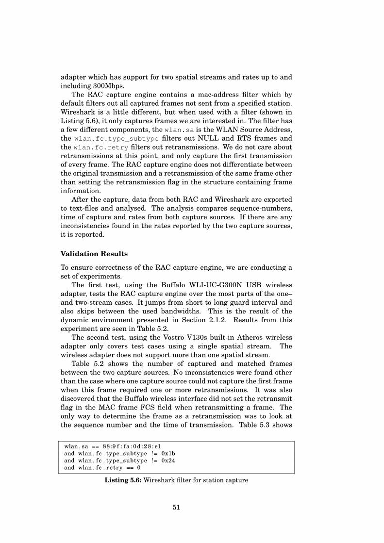
adapter which has support for two spatial streams and rates up to andincluding 300Mbps.

The RAC capture engine contains a mac-address filter which bydefault filters out all captured frames not sent from a specified station.Wireshark is a little different, but when used with a filter (shown inListing 5.6), it only captures frames we are interested in. The filter hasa few different components, the wlan.sa is the WLAN Source Address,the wlan.fc.type_subtype filters out NULL and RTS frames andthe wlan.fc.retry filters out retransmissions. We do not care aboutretransmissions at this point, and only capture the first transmissionof every frame. The RAC capture engine does not differentiate betweenthe original transmission and a retransmission of the same frame otherthan setting the retransmission flag in the structure containing frameinformation.

After the capture, data from both RAC and Wireshark are exportedto text-files and analysed. The analysis compares sequence-numbers,time of capture and rates from both capture sources. If there are anyinconsistencies found in the rates reported by the two capture sources,it is reported.

Validation Results

To ensure correctness of the RAC capture engine, we are conducting aset of experiments.

The first test, using the Buffalo WLI-UC-G300N USB wirelessadapter, tests the RAC capture engine over the most parts of the one–and two-stream cases. It jumps from short to long guard interval andalso skips between the used bandwidths. This is the result of thedynamic environment presented in Section 2.1.2. Results from thisexperiment are seen in Table 5.2.

The second test, using the Vostro V130s built-in Atheros wirelessadapter only covers test cases using a single spatial stream. Thewireless adapter does not support more than one spatial stream.

Table 5.2 shows the number of captured and matched framesbetween the two capture sources. No inconsistencies were found otherthan the case where one capture source could not capture the first framewhen this frame required one or more retransmissions. It was alsodiscovered that the Buffalo wireless interface did not set the retransmitflag in the MAC frame FCS field when retransmitting a frame. Theonly way to determine the frame as a retransmission was to look atthe sequence number and the time of transmission. Table 5.3 shows

wlan . sa == 88:9 f : fa :0d : 2 8 : e1and wlan . f c . type_subtype != 0x1band wlan . f c . type_subtype != 0x24and wlan . f c . retry == 0

Listing 5.6: Wireshark filter for station capture

51

the results from the rate-validation tests performed on the Dell VostroV130. Again, both capture sources reported the same bit-rate andsequence number.

5.3 Packet Classification Engine

Captured packets have to be classified in the current context of thecapturing process. There are several types of behaviours we are lookingfor when trying to classify the different rate adoption algorithms.

• sampling events

• best rate change

• retransmission

• RTS/CTS

5.3.1 Sampling Events

Sampling happens when the RAA decides to send a frame with adifferent rate than the current best rate in order to probe for changesin the wireless channel. To be able to determine whether a packet is asampling packet, we need to analyse at least three consecutive packets.

We start by defining a sampling event as an event where, amongstthree consecutive frames, the middle frame is sent with a different ratethan the first and the third frame, see Figure 5.1. As the captureprocess is lossy, one cannot always capture three consecutive framestravelling over the wireless channel. Another issue is when a samplingevent occurs immediately before a best-rate change in the RAA. Thisis shown in Figure 5.2, where the RAA changes its current best rateimmediately following a sampling event. In this figure, frame 100 istransmitted using the current best rate of rate A, followed by a samplingframe transmitted using rate B. The RAA, in this case, runs its best-rate calculation immediately following frame 101, decides that rate Bis better than rate A, and changes its current best rate to B. Thus, thisevent is not considered to be a sampling event by the analysis part,even though it is a sampling event for the RAA. Being able to classifythis as a sampling event is hard. One can, in SampleRate’s case, assumethe event to be a sampling event by using knowledge about the RAA, itsfrequent and predictable sampling characteristics, but this would resultin an assumption that is not necessarily true as one cannot assumethe RAA to be SampleRate without prior knowledge about the station’sdriver. Listing 5.7 shows pseudo-code for detecting a sample event. Thiscode represents Figure 5.1 where there are three consecutive capturedframes with the rate of the middle frame being different from the firstand the third.

52

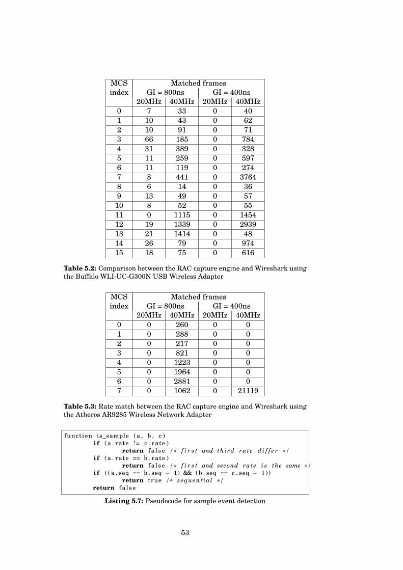
MCS Matched framesindex GI = 800ns GI = 400ns

20MHz 40MHz 20MHz 40MHz0 7 33 0 401 10 43 0 622 10 91 0 713 66 185 0 7844 31 389 0 3285 11 259 0 5976 11 119 0 2747 8 441 0 37648 6 14 0 369 13 49 0 57

10 8 52 0 5511 0 1115 0 145412 19 1339 0 293913 21 1414 0 4814 26 79 0 97415 18 75 0 616

Table 5.2: Comparison between the RAC capture engine and Wireshark usingthe Buffalo WLI-UC-G300N USB Wireless Adapter

MCS Matched framesindex GI = 800ns GI = 400ns

20MHz 40MHz 20MHz 40MHz0 0 260 0 01 0 288 0 02 0 217 0 03 0 821 0 04 0 1223 0 05 0 1964 0 06 0 2881 0 07 0 1062 0 21119

Table 5.3: Rate match between the RAC capture engine and Wireshark usingthe Atheros AR9285 Wireless Network Adapter

function is_sample ( a , b , c )i f ( a . rate != c . rate )

return f a l se /* f i r s t and third rate d i f f e r */i f ( a . rate == b . rate )

return f a l se /* f i r s t and second rate i s the same */i f ( ( a . seq == b . seq − 1) && ( b . seq == c . seq − 1 ) )

return true /* sequential */return f a l se

Listing 5.7: Pseudocode for sample event detection

53

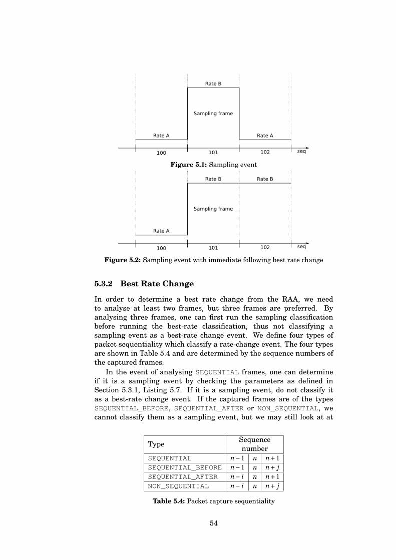
Figure 5.1: Sampling event

Figure 5.2: Sampling event with immediate following best rate change

5.3.2 Best Rate Change

In order to determine a best rate change from the RAA, we needto analyse at least two frames, but three frames are preferred. Byanalysing three frames, one can first run the sampling classificationbefore running the best-rate classification, thus not classifying asampling event as a best-rate change event. We define four types ofpacket sequentiality which classify a rate-change event. The four typesare shown in Table 5.4 and are determined by the sequence numbers ofthe captured frames.

In the event of analysing SEQUENTIAL frames, one can determineif it is a sampling event by checking the parameters as defined inSection 5.3.1, Listing 5.7. If it is a sampling event, do not classify itas a best-rate change event. If the captured frames are of the typesSEQUENTIAL_BEFORE, SEQUENTIAL_AFTER or NON_SEQUENTIAL, wecannot classify them as a sampling event, but we may still look at at

Type Sequencenumber

SEQUENTIAL n −1 n n +1SEQUENTIAL_BEFORE n −1 n n + jSEQUENTIAL_AFTER n − i n n +1NON_SEQUENTIAL n − i n n + j

Table 5.4: Packet capture sequentiality

54

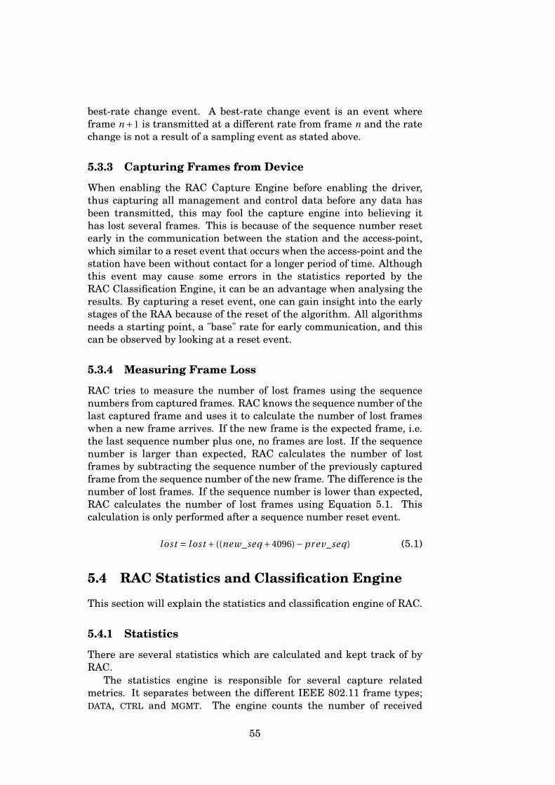
best-rate change event. A best-rate change event is an event whereframe n +1 is transmitted at a different rate from frame n and the ratechange is not a result of a sampling event as stated above.

5.3.3 Capturing Frames from Device

When enabling the RAC Capture Engine before enabling the driver,thus capturing all management and control data before any data hasbeen transmitted, this may fool the capture engine into believing ithas lost several frames. This is because of the sequence number resetearly in the communication between the station and the access-point,which similar to a reset event that occurs when the access-point and thestation have been without contact for a longer period of time. Althoughthis event may cause some errors in the statistics reported by theRAC Classification Engine, it can be an advantage when analysing theresults. By capturing a reset event, one can gain insight into the earlystages of the RAA because of the reset of the algorithm. All algorithmsneeds a starting point, a "base" rate for early communication, and thiscan be observed by looking at a reset event.

5.3.4 Measuring Frame Loss

RAC tries to measure the number of lost frames using the sequencenumbers from captured frames. RAC knows the sequence number of thelast captured frame and uses it to calculate the number of lost frameswhen a new frame arrives. If the new frame is the expected frame, i.e.the last sequence number plus one, no frames are lost. If the sequencenumber is larger than expected, RAC calculates the number of lostframes by subtracting the sequence number of the previously capturedframe from the sequence number of the new frame. The difference is thenumber of lost frames. If the sequence number is lower than expected,RAC calculates the number of lost frames using Equation 5.1. Thiscalculation is only performed after a sequence number reset event.

lost = l ost + ((new_seq +4096)−pr ev_seq) (5.1)

5.4 RAC Statistics and Classification Engine

This section will explain the statistics and classification engine of RAC.

5.4.1 Statistics

There are several statistics which are calculated and kept track of byRAC.

The statistics engine is responsible for several capture relatedmetrics. It separates between the different IEEE 802.11 frame types;DATA, CTRL and MGMT. The engine counts the number of received

55

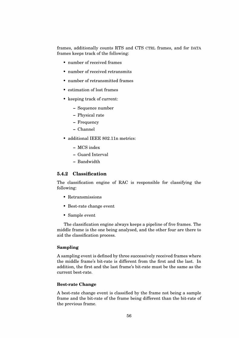
frames, additionally counts RTS and CTS CTRL frames, and for DATAframes keeps track of the following:

• number of received frames

• number of received retransmits

• number of retransmitted frames

• estimation of lost frames

• keeping track of current:

– Sequence number

– Physical rate

– Frequency

– Channel

• additional IEEE 802.11n metrics:

– MCS index

– Guard Interval

– Bandwidth

5.4.2 Classification

The classification engine of RAC is responsible for classifying thefollowing:

• Retransmissions

• Best-rate change event

• Sample event

The classification engine always keeps a pipeline of five frames. Themiddle frame is the one being analysed, and the other four are there toaid the classification process.

Sampling

A sampling event is defined by three successively received frames wherethe middle frame’s bit-rate is different from the first and the last. Inaddition, the first and the last frame’s bit-rate must be the same as thecurrent best-rate.

Best-rate Change

A best-rate change event is classified by the frame not being a sampleframe and the bit-rate of the frame being different than the bit-rate ofthe previous frame.

56

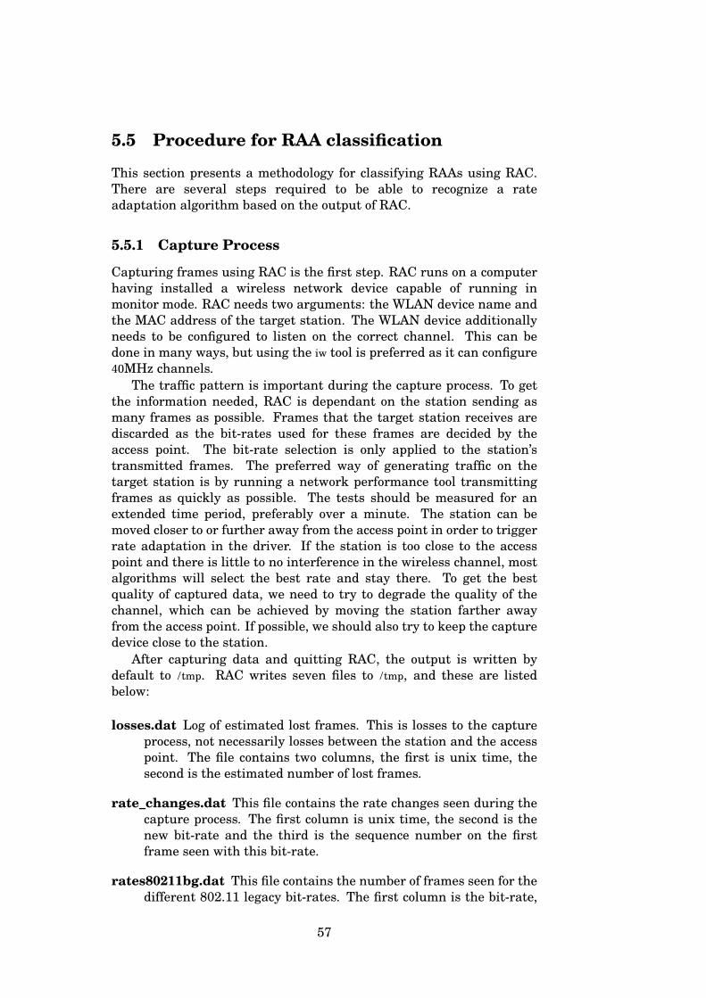
5.5 Procedure for RAA classification

This section presents a methodology for classifying RAAs using RAC.There are several steps required to be able to recognize a rateadaptation algorithm based on the output of RAC.

5.5.1 Capture Process

Capturing frames using RAC is the first step. RAC runs on a computerhaving installed a wireless network device capable of running inmonitor mode. RAC needs two arguments: the WLAN device name andthe MAC address of the target station. The WLAN device additionallyneeds to be configured to listen on the correct channel. This can bedone in many ways, but using the iw tool is preferred as it can configure40MHz channels.

The traffic pattern is important during the capture process. To getthe information needed, RAC is dependant on the station sending asmany frames as possible. Frames that the target station receives arediscarded as the bit-rates used for these frames are decided by theaccess point. The bit-rate selection is only applied to the station’stransmitted frames. The preferred way of generating traffic on thetarget station is by running a network performance tool transmittingframes as quickly as possible. The tests should be measured for anextended time period, preferably over a minute. The station can bemoved closer to or further away from the access point in order to triggerrate adaptation in the driver. If the station is too close to the accesspoint and there is little to no interference in the wireless channel, mostalgorithms will select the best rate and stay there. To get the bestquality of captured data, we need to try to degrade the quality of thechannel, which can be achieved by moving the station farther awayfrom the access point. If possible, we should also try to keep the capturedevice close to the station.

After capturing data and quitting RAC, the output is written bydefault to /tmp. RAC writes seven files to /tmp, and these are listedbelow:

losses.dat Log of estimated lost frames. This is losses to the captureprocess, not necessarily losses between the station and the accesspoint. The file contains two columns, the first is unix time, thesecond is the estimated number of lost frames.

rate_changes.dat This file contains the rate changes seen during thecapture process. The first column is unix time, the second is thenew bit-rate and the third is the sequence number on the firstframe seen with this bit-rate.

rates80211bg.dat This file contains the number of frames seen for thedifferent 802.11 legacy bit-rates. The first column is the bit-rate,

57

the second is the number of frames and the last is the frame countin percent to the total number of frames.

rates80211n.dat This file contains the distribution of IEEE 802.11nframes seen, it has five columns with data. The first is the MCSindex (see Section 2.4 on page 16 for more information). Thesecond and third column is the number of captured frames for thelong Guard Interval (GI) frames in 20MHz and 40MHz channelwidths. Columns four and five represent the number of framesreceived for the short GI 20MHz and 40MHz channel widths.

retries.dat This file contains captured retransmission rates. The filecontains the time, the original bit-rate and the bit-rate of theretransmitted frames. The first column is unix time, the secondis the total number of retransmissions, the third column is theoriginal frame’s bit-rate and the remaining columns are the bit-rates of every retransmission following the original. If a framehas been retransmitted four times, there will be four columnsfollowing the three first.

samples.dat This file contains captured samples. The file structureis unix time in the first column and the bit-rate of the capturedsample in the second.

statistics.dat This file is a dump of the statistics kept by RAC. Theseare:

• Number of captured frames

• Estimated lost frames

• Captured retransmits

• Loss ratio

• Total number of rate changes

• How many rate changes with a change of more than one ratestep

• Maximum rate changes per second

• Minimum time between rate changes

• Minimum number of frames between rate changes

• Total number of samples

• Sampling ratio

• Minimum number of frames between samples

• Number of RTS frames

• Number of CTS frames

• Maximum number of retransmissions for a single frame

58

5.5.2 Analysis

Analysing the captured data is the next step in classifying observedtraffic. By using the output of RAC from the capture process, we willsystematically look at the captured data.

The statistics .dat file contains most of the information we need. Wewill use this file to figure out if the observed algorithm uses RTS/CTS,sampling (and the sampling ratio), rate jumping and determine themaximum number of observed retransmissions for a frame. The filealso contains the maximum number of rate changes per second and theminimum time between rate changes.

To determine the retransmission strategy used, we need to use theretries .dat file. By looking at the bit-rates for frames needing the mostretransmissions and comparing this to the defined strategies seen inSection 4.2, we can determine the retransmission strategy.

Excluded rates can be determined by looking at the rate distributionin rates80211bg.dat. If we see zero frames being transmitted using the9Mbps rate, but there are several frames being sent at both 6Mbps and11Mbps, we can assume an exclusion of the 9Mbps rate.

To figure out the starting rate, we need to locate events where theRAA is being reset. There are mainly two events which cause the RAAto be reset. When the station connects to an access point and whenthe driver is being reset because of a temporary disruption in networkconnectivity. By observing the rate changes immediately after eventsuch as these, we may be able to determine the starting rate. The mosteffective way is to run the capture process when connecting a station tothe access point.

5.5.3 Comparison

Finally, we compare our results to metrics gathered by researchand previously measured values. In Section 4.1, we have gatheredinformation about the RAAs present in the madwifi driver and inSection 8.1, we will present measurements of the same driver.

There are measurements which weigh more than others. The retrystrategy, for example, is one of the most important measurements.Below is a list of measured ranging from the most important at thetop to the least important at the bottom.

• Retry strategy and max retries

– From our research, we see a big difference in how thedifferent algorithms handle retransmissions.

• Rate jumping

– Rate jumping is the main separator between madwifistwo least advanced RAAs (AMRR and Onoe) and the twoadvanced RAAs, SampleRate and Minstrel.

59

• Max rate changes per second and minimum time between ratechanges

– This metric is very dependent on how fast the algorithmreacts to changes in the wireless channel.

• Sampling rate

– SampleRate and Minstrel can be separated by looking at thisvalue.

• Starting rate

– Different algorithms choose the bit-rate of the first framebased on different rules. Some chose the rate from a statictable, others, i.e. SampleRate choose the bit-rate of thefirst frame based on the Signal-To-Noise (SNR) ratio of thewireless channel.

• Excluded rates

– We know that SampleRate never used the 9Mbps rate.

• Use RTS/CTS

– Some algorithms may use RTS/CTS when communicatingwith other wireless devices.

After weighing the different metrics against each other, it should bepossible to classify observed traffic against a known RAA.

Summary

This section presented the design and implementation of the Rate Adap-tation Classifier and a method of classifying rate adaptation algorithmsby using the output from said tool. We have presented a thorough workon fingerprinting RAAs implemented in the madwifi driver and identi-fied important metrics and behaviour of the algorithms. We have ex-plained the implementation of RAC and finally explained the outputgenerated by RAC and how to use this output when trying to classifyalgorithms. The next part of this thesis will show how we use the tooland method presented here in order to validate its effectiveness.

60

Part IV

Experimental setup

61

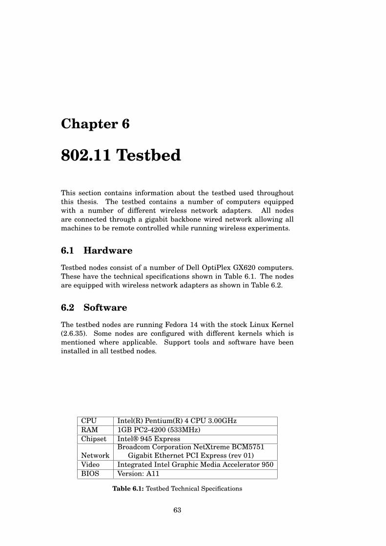
Chapter 6

802.11 Testbed

This section contains information about the testbed used throughoutthis thesis. The testbed contains a number of computers equippedwith a number of different wireless network adapters. All nodesare connected through a gigabit backbone wired network allowing allmachines to be remote controlled while running wireless experiments.

6.1 Hardware

Testbed nodes consist of a number of Dell OptiPlex GX620 computers.These have the technical specifications shown in Table 6.1. The nodesare equipped with wireless network adapters as shown in Table 6.2.

6.2 Software

The testbed nodes are running Fedora 14 with the stock Linux Kernel(2.6.35). Some nodes are configured with different kernels which ismentioned where applicable. Support tools and software have beeninstalled in all testbed nodes.

CPU Intel(R) Pentium(R) 4 CPU 3.00GHzRAM 1GB PC2-4200 (533MHz)Chipset Intel® 945 Express

NetworkBroadcom Corporation NetXtreme BCM5751

Gigabit Ethernet PCI Express (rev 01)Video Integrated Intel Graphic Media Accelerator 950BIOS Version: A11

Table 6.1: Testbed Technical Specifications

63

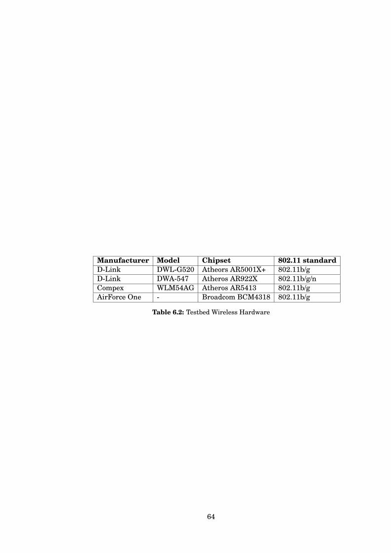
Manufacturer Model Chipset 802.11 standardD-Link DWL-G520 Atheors AR5001X+ 802.11b/gD-Link DWA-547 Atheros AR922X 802.11b/g/nCompex WLM54AG Atheros AR5413 802.11b/gAirForce One - Broadcom BCM4318 802.11b/g

Table 6.2: Testbed Wireless Hardware

64

Chapter 7

Experiment

This chapter contains details about the experiments conducted in thisthesis. The main experiment are the validation tests run on the madwifirate adaptation algorithms.

The madwifi driver is the driver previously used for most of theAtheros Wireless Network Cards. The rate adaptation algorithmsimplemented in this driver are Onoe, AMRR, SampleRate and Minstrel.

In our experiments, we will use madwifi driver version svn r4180.This is a custom compiled driver used in a Fedora 14 system runningthe Linux Kernel 2.6.35.

7.1 Test Details

These tests have been conducted using a variety of different machinesand wireless interface cards. The main goal of these experiments is tocompare the observed behaviour of open-source drivers to the expectedtheoretical behaviour of the same driver. By using the results from theseinitial experiments, we are better equipped to analyse the behaviour ofother drivers which may be proprietary and where no source code havebeen released by the manufacturer of the product.

To ensure correct results from the madwifi validation tests, twotypes of tests were conducted, a stationary and one moving. Thestationary tests were conducted in order to observe the algorithms ina semi-stable environment, while the moving tests were conducted inorder to observe the algorithms in a highly changing environment. Themoving tests were done using the natural structure of the forth floorof the Informatics building at the University of Oslo. The test wereconducted using a moving AP and a stationary station. This becauseof the difficulty of moving the station wireless hardware. By movingthe AP, we could perform the tests using a normal laptop running onbatteries while walking with the device around the facility. The route ofthe moving AP is as shown in Figure 7.2.

The stationary tests were conducted by fixing the Access Point inan office down the hall from the lab. Both the stations and the APwere fixed during all the stationary experiments. The distance between

65

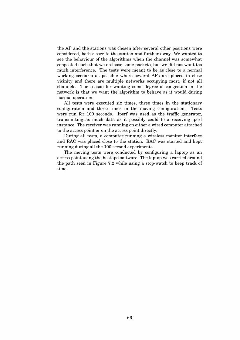
the AP and the stations was chosen after several other positions wereconsidered, both closer to the station and further away. We wanted tosee the behaviour of the algorithms when the channel was somewhatcongested such that we do loose some packets, but we did not want toomuch interference. The tests were meant to be as close to a normalworking scenario as possible where several APs are placed in closevicinity and there are multiple networks occupying most, if not allchannels. The reason for wanting some degree of congestion in thenetwork is that we want the algorithm to behave as it would duringnormal operation.

All tests were executed six times, three times in the stationaryconfiguration and three times in the moving configuration. Testswere run for 100 seconds. Iperf was used as the traffic generator,transmitting as much data as it possibly could to a receiving iperfinstance. The receiver was running on either a wired computer attachedto the access point or on the access point directly.

During all tests, a computer running a wireless monitor interfaceand RAC was placed close to the station. RAC was started and keptrunning during all the 100 second experiments.

The moving tests were conducted by configuring a laptop as anaccess point using the hostapd software. The laptop was carried aroundthe path seen in Figure 7.2 while using a stop-watch to keep track oftime.

66

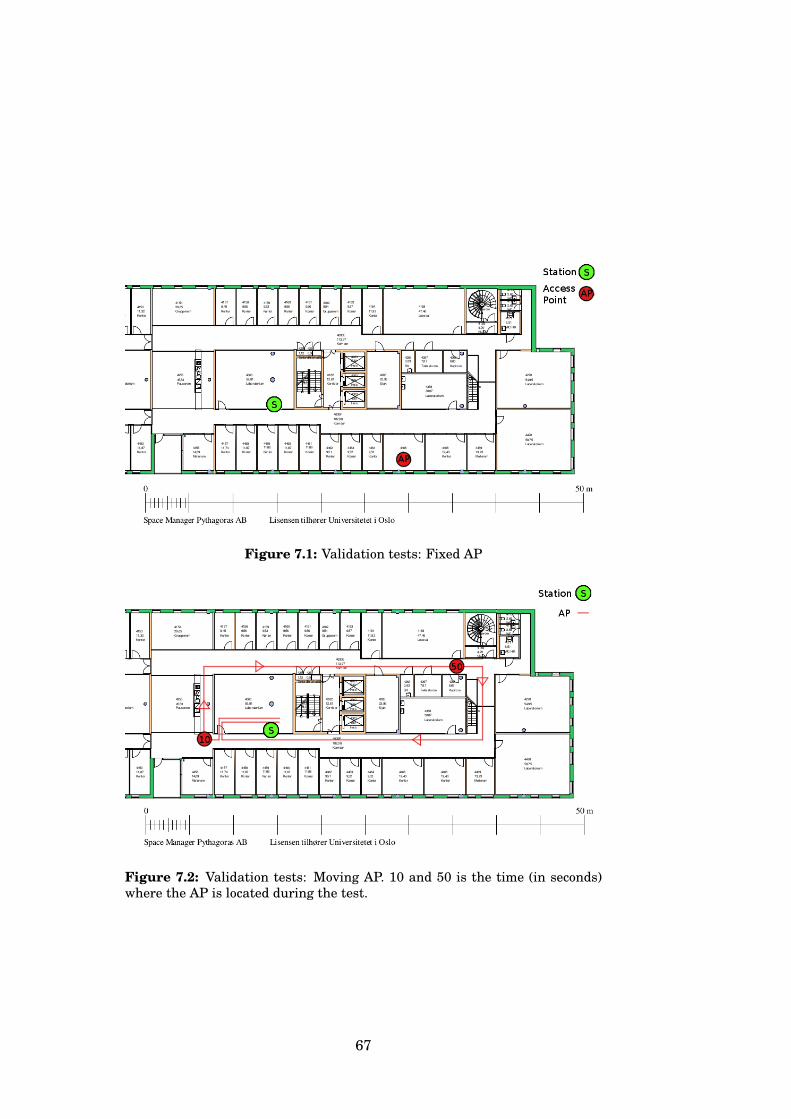
Figure 7.1: Validation tests: Fixed AP

Figure 7.2: Validation tests: Moving AP. 10 and 50 is the time (in seconds)where the AP is located during the test.

67

Part V

Evaluation Results

69

Chapter 8

Classifying KnownAlgorithms

In this section we will present tests of RAC using different wirelesshardware and drivers.

8.1 Madwifi validation tests

This section contains results from validation tests conducted on themadwifi driver for Atheros based chipsets. All algorithms, AMRR,Onoe, SampleRate and Minstrel have been tested and validated againstexpected results.

8.1.1 Analysing AMRR

Using knowledge from Part II, we will run a set of tests and observehow the driver behaves. We will try to match this with the previouslyresearched behaviour of the algorithm.

First, we will analyse the retry chain of AMRR. The AMRR retrychain is built based on the information from Table 4.3 on page 34 whichstates that the AMRR algorithm populates the retry chain using thefollowing rules:

1. current best rate/once

2. next lower rate/once

3. next next lower rate/once

4. lowest base rate/once

We would expect to see this behaviour when trying to fingerprint AMRRin our experiments. Listing 8.1 shows several snippets of the resultfile generated by RAC when capturing iperf traffic governed by thealgorithm. The file contains three or more columns of information,starting with the time-stamp of when the original frame was receivedin the first column. The next column contains the total number of

71

retransmissions and the third column contains the physical rate of theoriginally transmitted frame. The next n columns contains the physicalrate of the retransmitted frames, and if no losses occurred in the captureprocess, one line in this file represents the current retry chain untilthe frame is either transmitted successfully or discarded following theinformation set in the retry chain.

As expected, the retry chain is populated using AMRRs procedureas shown in the list above. Starting from the top of the results, we canconfirm that when the current best rate is 18Mbps, the retry chain ispopulated as shown in Table 8.1. Following the results in Listing 8.1,we see that the behaviour of the retries follows the same structure asthe result in line 1 of Listing 8.1. We also see that, when the currentbest rate is 5.5Mbps or lower, there are not enough rates to choose fromwhen populating the retry chain, and hence, the retry chain is not fullyutilized. When the original frame is transmitted using 5.5Mbps, theretry chain is populated as seen in Table 8.2. As the current best ratefalls even lower, the retry chain is populated using fewer and fewerrecords until the current best rate is 1Mbps, in which case there areno retries.

Analysing AMRRs rate changes is the second step in decipheringAMRR governed traffic. Using RAC, we have captured all rate changesduring 100 second upload experiments. We see from Figure 8.1 howAMRR behaves in our validation tests. The main confirmation we getfrom these results is the behaviour of AMRR when changing the bestrate. AMRR is expected to change rates one rate-index at a time,and this is seen in Figure 8.1. We observe AMRR fluctuating strongly,especially in the moving tests, see Figure 8.1(a) where we have spikesin the graph. This is because of the driver reconnecting to the APwhen loosing connectivity over a predetermined length of time. If theconnection is having difficulties exchanging packets at 1Mbps and thedriver is struggling with management packets, the connection is resetand the session is renegotiated. The selected RAA is then notified bythe reset event and the algorithm is reset. Although the reset code isdependent on the implementation on the algorithm, all algorithms inthe madwifi driver reset the algorithm to the initial state. AMRR neverchanges best rate directly from 1Mbps to 36Mbps, but 36Mbps is thedefault starting rate in madwifis implementation of AMRR.

In addition to the rate changes observed by RAC, we have includedthe statistics output created by the application. RAC creates somesimple statistics, see Section 5.4.1 on page 55, and this can be usedwhen analysing RAAs. We see from the statistics of AMRR shown inTable 8.3 that AMRR at most changed rate twice a second and that,as expected, it does not use sampling, it does not jump rates whenchanging best-rate, and it has at maximum three retry attempts. Theminimum time between rate changes is reported to be 397ms which is abit more frequent than we expect from the implementation. We did notspend time trying to uncover why we see this discrepancy between theimplementation and the captured data.

72

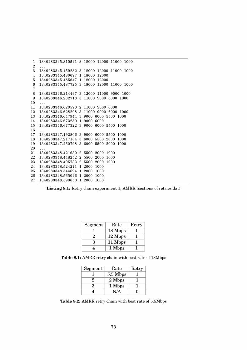
1 1340283345.310541 3 18000 12000 11000 10002 . . .3 1340283345.459232 3 18000 12000 11000 10004 1340283345.480697 1 18000 120005 1340283345.485647 1 18000 120006 1340283345.487725 3 18000 12000 11000 10007 . . .8 1340283346.214497 3 12000 11000 9000 10009 1340283346.232713 3 11000 9000 6000 1000

10 . . .11 1340283346.620590 2 11000 9000 600012 1340283346.628298 3 11000 9000 6000 100013 1340283346.647944 3 9000 6000 5500 100014 1340283346.673280 1 9000 600015 1340283346.677322 3 9000 6000 5500 100016 . . .17 1340283347.192806 3 9000 6000 5500 100018 1340283347.217184 3 6000 5500 2000 100019 1340283347.250798 3 6000 5500 2000 100020 . . .21 1340283348.421630 2 5500 2000 100022 1340283348.448252 2 5500 2000 100023 1340283348.495733 2 5500 2000 100024 1340283348.524271 1 2000 100025 1340283348.544694 1 2000 100026 1340283348.565046 1 2000 100027 1340283348.590650 1 2000 1000

Listing 8.1: Retry chain experiment 1, AMRR (sections of retries.dat)

Segment Rate Retry1 18 Mbps 12 12 Mbps 13 11 Mbps 14 1 Mbps 1

Table 8.1: AMRR retry chain with best rate of 18Mbps

Segment Rate Retry1 5.5 Mbps 12 2 Mbps 13 1 Mbps 14 N/A 0

Table 8.2: AMRR retry chain with best rate of 5.5Mbps

73

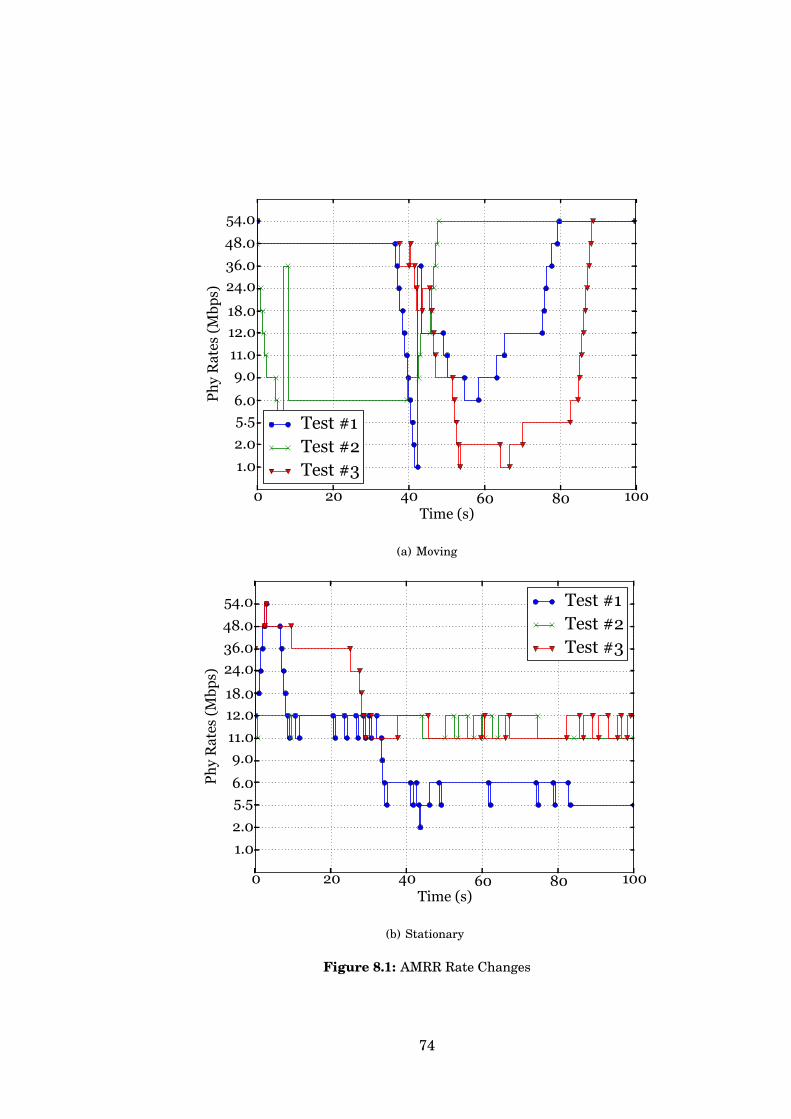
0 20 40 60 80 100Time (s)

1.0

2.0

5.56.0

9.0

11.0

12.0

18.0

24.0

36.0

48.0

54.0P

hy

Rat

es (

Mbp

s)

Test #1Test #2Test #3

(a) Moving

0 20 40 60 80 100Time (s)

1.0

2.0

5.56.0

9.0

11.0

12.0

18.0

24.0

36.0

48.0

54.0

Ph

y R

ates

(M

bps)


(b) Stationary

Figure 8.1: AMRR Rate Changes

74

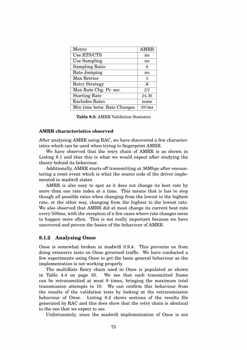
Metric AMRRUse RTS/CTS noUse Sampling noSampling Ratio 0Rate Jumping noMax Retries 3Retry Strategy AMax Rate Chg. Pr. sec. 2/2Starting Rate 24,36Excludes Rates noneMin time betw. Rate Changes 397ms

Table 8.3: AMRR Validation Statistics

AMRR characteristics observed

After analysing AMRR using RAC, we have discovered a few character-istics which can be used when trying to fingerprint AMRR.

We have observed that the retry chain of AMRR is as shown inListing 8.1 and that this is what we would expect after studying thetheory behind its behaviour.

Additionally, AMRR starts off transmitting at 36Mbps after encoun-tering a reset event which is what the source code of the driver imple-mented in madwifi states.

AMRR is also easy to spot as it does not change its best rate bymore than one rate index at a time. This means that is has to stepthough all possible rates when changing from the lowest to the highestrate, or the other way, changing from the highest to the lowest rate.We also observed that AMRR did at most change its current best rateevery 500ms, with the exception of a few cases where rate changes seemto happen more often. This is not really important because we haveuncovered and proven the basics of the behaviour of AMRR.

8.1.2 Analysing Onoe

Onoe is somewhat broken in madwifi 0.9.4. This prevents us fromdoing extensive tests on Onoe governed traffic. We have conducted afew experiments using Onoe to get the basic general behaviour as theimplementation is not working properly.

The multiRate Retry chain used in Onoe is populated as shownin Table 4.4 on page 35. We see that each transmitted framecan be retransmitted at most 9 times, bringing the maximum totaltransmission attempts to 10. We can confirm this behaviour fromthe results of the validation tests by looking at the retransmissionbehaviour of Onoe. Listing 8.2 shows sections of the results filegenerated by RAC and this does show that the retry chain is identicalto the one that we expect to see.

Unfortunately, since the madwifi implementation of Onoe is not

75

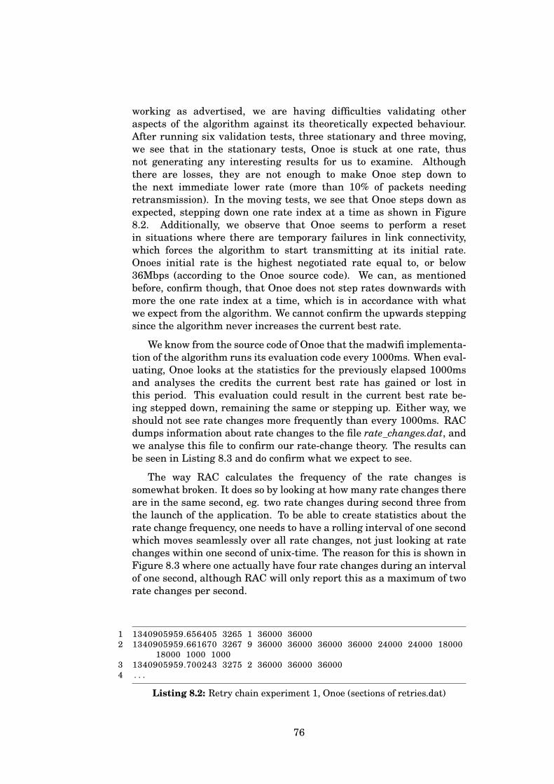
working as advertised, we are having difficulties validating otheraspects of the algorithm against its theoretically expected behaviour.After running six validation tests, three stationary and three moving,we see that in the stationary tests, Onoe is stuck at one rate, thusnot generating any interesting results for us to examine. Althoughthere are losses, they are not enough to make Onoe step down tothe next immediate lower rate (more than 10% of packets needingretransmission). In the moving tests, we see that Onoe steps down asexpected, stepping down one rate index at a time as shown in Figure8.2. Additionally, we observe that Onoe seems to perform a resetin situations where there are temporary failures in link connectivity,which forces the algorithm to start transmitting at its initial rate.Onoes initial rate is the highest negotiated rate equal to, or below36Mbps (according to the Onoe source code). We can, as mentionedbefore, confirm though, that Onoe does not step rates downwards withmore the one rate index at a time, which is in accordance with whatwe expect from the algorithm. We cannot confirm the upwards steppingsince the algorithm never increases the current best rate.

We know from the source code of Onoe that the madwifi implementa-tion of the algorithm runs its evaluation code every 1000ms. When eval-uating, Onoe looks at the statistics for the previously elapsed 1000msand analyses the credits the current best rate has gained or lost inthis period. This evaluation could result in the current best rate be-ing stepped down, remaining the same or stepping up. Either way, weshould not see rate changes more frequently than every 1000ms. RACdumps information about rate changes to the file rate_changes.dat, andwe analyse this file to confirm our rate-change theory. The results canbe seen in Listing 8.3 and do confirm what we expect to see.

The way RAC calculates the frequency of the rate changes issomewhat broken. It does so by looking at how many rate changes thereare in the same second, eg. two rate changes during second three fromthe launch of the application. To be able to create statistics about therate change frequency, one needs to have a rolling interval of one secondwhich moves seamlessly over all rate changes, not just looking at ratechanges within one second of unix-time. The reason for this is shown inFigure 8.3 where one actually have four rate changes during an intervalof one second, although RAC will only report this as a maximum of tworate changes per second.

1 1340905959.656405 3265 1 36000 360002 1340905959.661670 3267 9 36000 36000 36000 36000 24000 24000 18000

18000 1000 10003 1340905959.700243 3275 2 36000 36000 360004 . . .

Listing 8.2: Retry chain experiment 1, Onoe (sections of retries.dat)

76

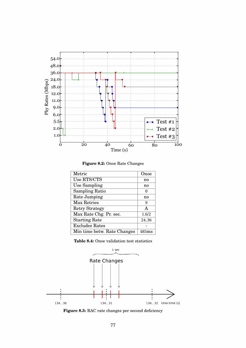
0 20 40 60 80 100Time (s)

1.0

2.0

5.56.0

9.0

11.0

12.0

18.0

24.0

36.0

48.0

54.0

Ph

y R

ates

(M

bps)


Figure 8.2: Onoe Rate Changes

Metric OnoeUse RTS/CTS noUse Sampling noSampling Ratio 0Rate Jumping noMax Retries 9Retry Strategy AMax Rate Chg. Pr. sec. 1.6/2Starting Rate 24,36Excludes Rates -Min time betw. Rate Changes 485ms

Table 8.4: Onoe validation test statistics

Figure 8.3: RAC rate changes per second deficiency

77

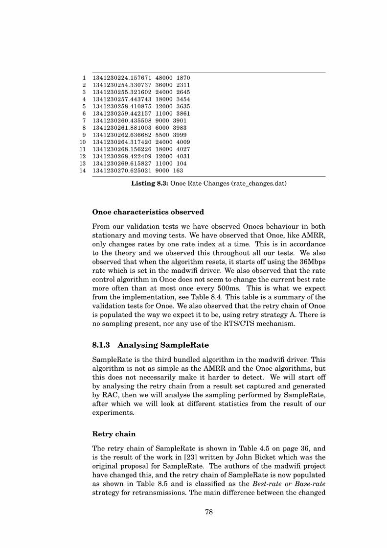
1 1341230224.157671 48000 18702 1341230254.330737 36000 23113 1341230255.321602 24000 26454 1341230257.443743 18000 34545 1341230258.410875 12000 36356 1341230259.442157 11000 38617 1341230260.435508 9000 39018 1341230261.881003 6000 39839 1341230262.636682 5500 3999

10 1341230264.317420 24000 400911 1341230268.156226 18000 402712 1341230268.422409 12000 403113 1341230269.615827 11000 10414 1341230270.625021 9000 163

Listing 8.3: Onoe Rate Changes (rate_changes.dat)

Onoe characteristics observed

From our validation tests we have observed Onoes behaviour in bothstationary and moving tests. We have observed that Onoe, like AMRR,only changes rates by one rate index at a time. This is in accordanceto the theory and we observed this throughout all our tests. We alsoobserved that when the algorithm resets, it starts off using the 36Mbpsrate which is set in the madwifi driver. We also observed that the ratecontrol algorithm in Onoe does not seem to change the current best ratemore often than at most once every 500ms. This is what we expectfrom the implementation, see Table 8.4. This table is a summary of thevalidation tests for Onoe. We also observed that the retry chain of Onoeis populated the way we expect it to be, using retry strategy A. There isno sampling present, nor any use of the RTS/CTS mechanism.

8.1.3 Analysing SampleRate

SampleRate is the third bundled algorithm in the madwifi driver. Thisalgorithm is not as simple as the AMRR and the Onoe algorithms, butthis does not necessarily make it harder to detect. We will start offby analysing the retry chain from a result set captured and generatedby RAC, then we will analyse the sampling performed by SampleRate,after which we will look at different statistics from the result of ourexperiments.

Retry chain

The retry chain of SampleRate is shown in Table 4.5 on page 36, andis the result of the work in [23] written by John Bicket which was theoriginal proposal for SampleRate. The authors of the madwifi projecthave changed this, and the retry chain of SampleRate is now populatedas shown in Table 8.5 and is classified as the Best-rate or Base-ratestrategy for retransmissions. The main difference between the changed

78

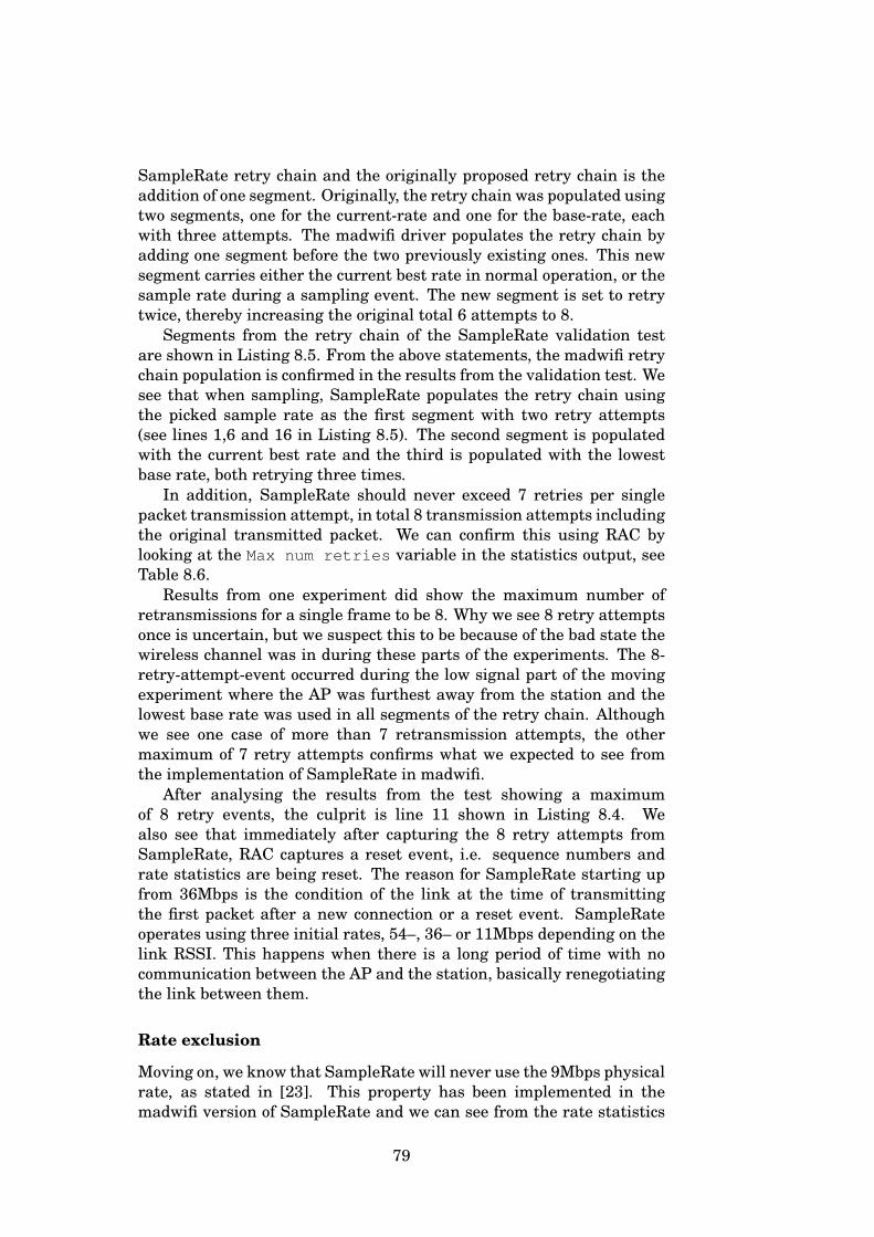
SampleRate retry chain and the originally proposed retry chain is theaddition of one segment. Originally, the retry chain was populated usingtwo segments, one for the current-rate and one for the base-rate, eachwith three attempts. The madwifi driver populates the retry chain byadding one segment before the two previously existing ones. This newsegment carries either the current best rate in normal operation, or thesample rate during a sampling event. The new segment is set to retrytwice, thereby increasing the original total 6 attempts to 8.

Segments from the retry chain of the SampleRate validation testare shown in Listing 8.5. From the above statements, the madwifi retrychain population is confirmed in the results from the validation test. Wesee that when sampling, SampleRate populates the retry chain usingthe picked sample rate as the first segment with two retry attempts(see lines 1,6 and 16 in Listing 8.5). The second segment is populatedwith the current best rate and the third is populated with the lowestbase rate, both retrying three times.

In addition, SampleRate should never exceed 7 retries per singlepacket transmission attempt, in total 8 transmission attempts includingthe original transmitted packet. We can confirm this using RAC bylooking at the Max num retries variable in the statistics output, seeTable 8.6.

Results from one experiment did show the maximum number ofretransmissions for a single frame to be 8. Why we see 8 retry attemptsonce is uncertain, but we suspect this to be because of the bad state thewireless channel was in during these parts of the experiments. The 8-retry-attempt-event occurred during the low signal part of the movingexperiment where the AP was furthest away from the station and thelowest base rate was used in all segments of the retry chain. Althoughwe see one case of more than 7 retransmission attempts, the othermaximum of 7 retry attempts confirms what we expected to see fromthe implementation of SampleRate in madwifi.

After analysing the results from the test showing a maximumof 8 retry events, the culprit is line 11 shown in Listing 8.4. Wealso see that immediately after capturing the 8 retry attempts fromSampleRate, RAC captures a reset event, i.e. sequence numbers andrate statistics are being reset. The reason for SampleRate starting upfrom 36Mbps is the condition of the link at the time of transmittingthe first packet after a new connection or a reset event. SampleRateoperates using three initial rates, 54–, 36– or 11Mbps depending on thelink RSSI. This happens when there is a long period of time with nocommunication between the AP and the station, basically renegotiatingthe link between them.

Rate exclusion

Moving on, we know that SampleRate will never use the 9Mbps physicalrate, as stated in [23]. This property has been implemented in themadwifi version of SampleRate and we can see from the rate statistics

79

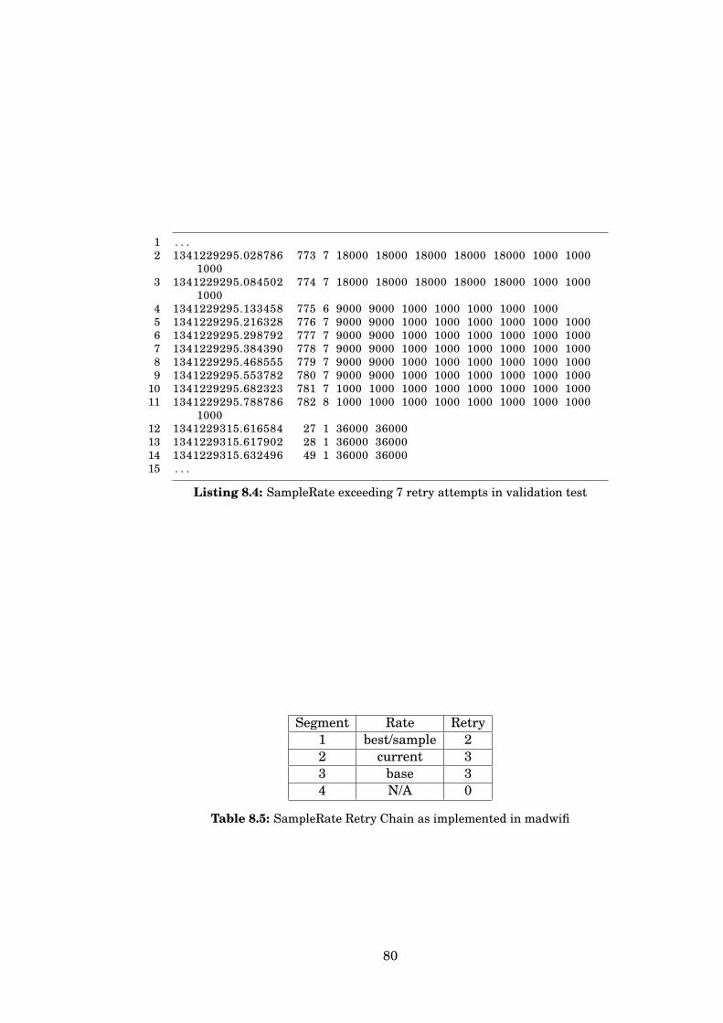
1 . . .2 1341229295.028786 773 7 18000 18000 18000 18000 18000 1000 1000

10003 1341229295.084502 774 7 18000 18000 18000 18000 18000 1000 1000

10004 1341229295.133458 775 6 9000 9000 1000 1000 1000 1000 10005 1341229295.216328 776 7 9000 9000 1000 1000 1000 1000 1000 10006 1341229295.298792 777 7 9000 9000 1000 1000 1000 1000 1000 10007 1341229295.384390 778 7 9000 9000 1000 1000 1000 1000 1000 10008 1341229295.468555 779 7 9000 9000 1000 1000 1000 1000 1000 10009 1341229295.553782 780 7 9000 9000 1000 1000 1000 1000 1000 1000

10 1341229295.682323 781 7 1000 1000 1000 1000 1000 1000 1000 100011 1341229295.788786 782 8 1000 1000 1000 1000 1000 1000 1000 1000

100012 1341229315.616584 27 1 36000 3600013 1341229315.617902 28 1 36000 3600014 1341229315.632496 49 1 36000 3600015 . . .

Listing 8.4: SampleRate exceeding 7 retry attempts in validation test

Segment Rate Retry1 best/sample 22 current 33 base 34 N/A 0

Table 8.5: SampleRate Retry Chain as implemented in madwifi

80

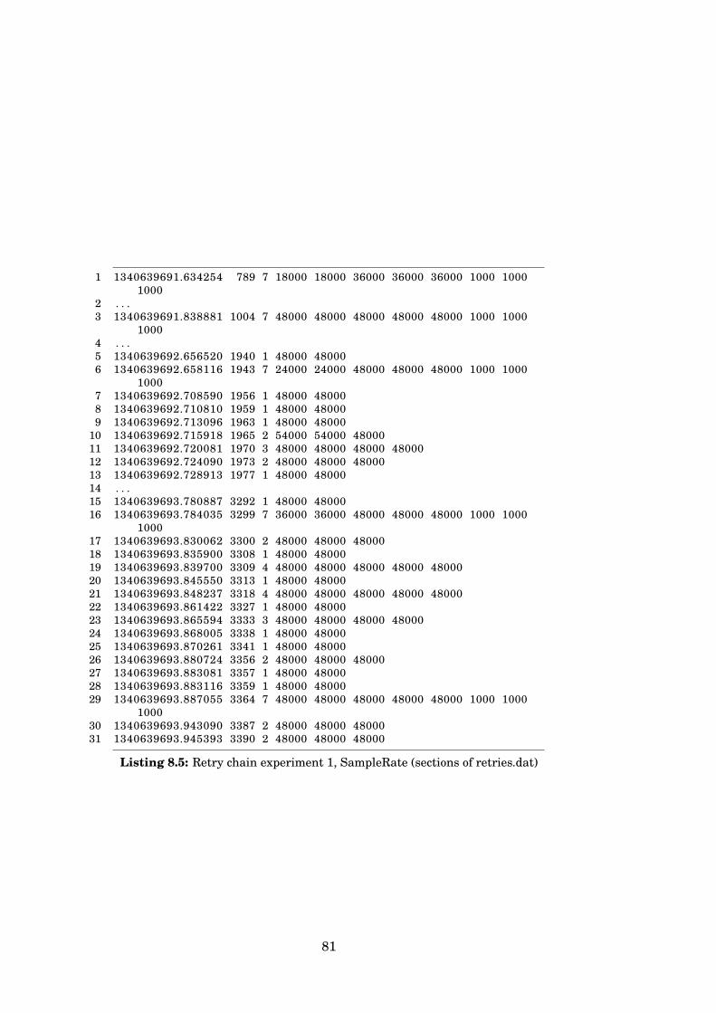
1 1340639691.634254 789 7 18000 18000 36000 36000 36000 1000 10001000

2 . . .3 1340639691.838881 1004 7 48000 48000 48000 48000 48000 1000 1000

10004 . . .5 1340639692.656520 1940 1 48000 480006 1340639692.658116 1943 7 24000 24000 48000 48000 48000 1000 1000

10007 1340639692.708590 1956 1 48000 480008 1340639692.710810 1959 1 48000 480009 1340639692.713096 1963 1 48000 48000

10 1340639692.715918 1965 2 54000 54000 4800011 1340639692.720081 1970 3 48000 48000 48000 4800012 1340639692.724090 1973 2 48000 48000 4800013 1340639692.728913 1977 1 48000 4800014 . . .15 1340639693.780887 3292 1 48000 4800016 1340639693.784035 3299 7 36000 36000 48000 48000 48000 1000 1000

100017 1340639693.830062 3300 2 48000 48000 4800018 1340639693.835900 3308 1 48000 4800019 1340639693.839700 3309 4 48000 48000 48000 48000 4800020 1340639693.845550 3313 1 48000 4800021 1340639693.848237 3318 4 48000 48000 48000 48000 4800022 1340639693.861422 3327 1 48000 4800023 1340639693.865594 3333 3 48000 48000 48000 4800024 1340639693.868005 3338 1 48000 4800025 1340639693.870261 3341 1 48000 4800026 1340639693.880724 3356 2 48000 48000 4800027 1340639693.883081 3357 1 48000 4800028 1340639693.883116 3359 1 48000 4800029 1340639693.887055 3364 7 48000 48000 48000 48000 48000 1000 1000

100030 1340639693.943090 3387 2 48000 48000 4800031 1340639693.945393 3390 2 48000 48000 48000

Listing 8.5: Retry chain experiment 1, SampleRate (sections of retries.dat)

81

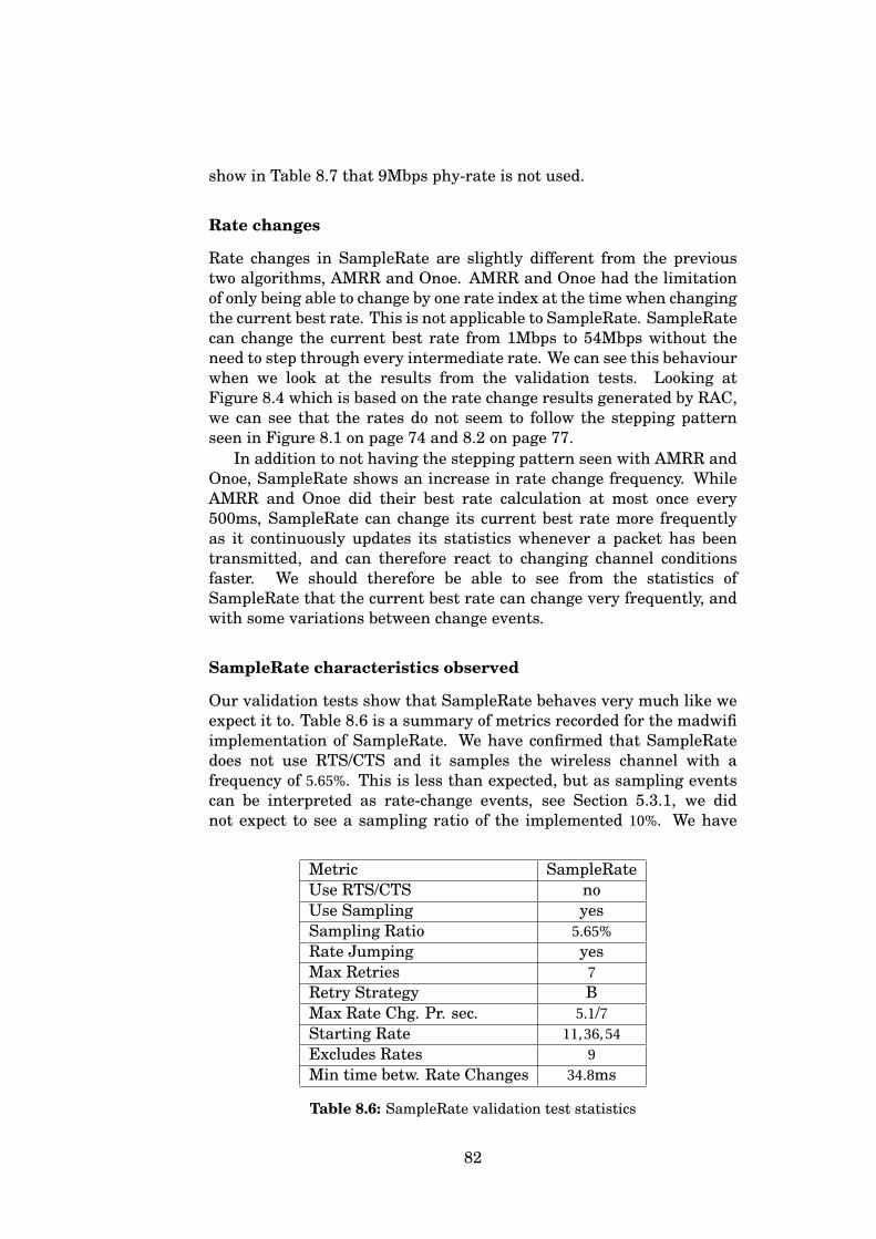
show in Table 8.7 that 9Mbps phy-rate is not used.

Rate changes

Rate changes in SampleRate are slightly different from the previoustwo algorithms, AMRR and Onoe. AMRR and Onoe had the limitationof only being able to change by one rate index at the time when changingthe current best rate. This is not applicable to SampleRate. SampleRatecan change the current best rate from 1Mbps to 54Mbps without theneed to step through every intermediate rate. We can see this behaviourwhen we look at the results from the validation tests. Looking atFigure 8.4 which is based on the rate change results generated by RAC,we can see that the rates do not seem to follow the stepping patternseen in Figure 8.1 on page 74 and 8.2 on page 77.

In addition to not having the stepping pattern seen with AMRR andOnoe, SampleRate shows an increase in rate change frequency. WhileAMRR and Onoe did their best rate calculation at most once every500ms, SampleRate can change its current best rate more frequentlyas it continuously updates its statistics whenever a packet has beentransmitted, and can therefore react to changing channel conditionsfaster. We should therefore be able to see from the statistics ofSampleRate that the current best rate can change very frequently, andwith some variations between change events.

SampleRate characteristics observed

Our validation tests show that SampleRate behaves very much like weexpect it to. Table 8.6 is a summary of metrics recorded for the madwifiimplementation of SampleRate. We have confirmed that SampleRatedoes not use RTS/CTS and it samples the wireless channel with afrequency of 5.65%. This is less than expected, but as sampling eventscan be interpreted as rate-change events, see Section 5.3.1, we didnot expect to see a sampling ratio of the implemented 10%. We have

Metric SampleRateUse RTS/CTS noUse Sampling yesSampling Ratio 5.65%Rate Jumping yesMax Retries 7Retry Strategy BMax Rate Chg. Pr. sec. 5.1/7Starting Rate 11,36,54Excludes Rates 9Min time betw. Rate Changes 34.8ms

Table 8.6: SampleRate validation test statistics

82

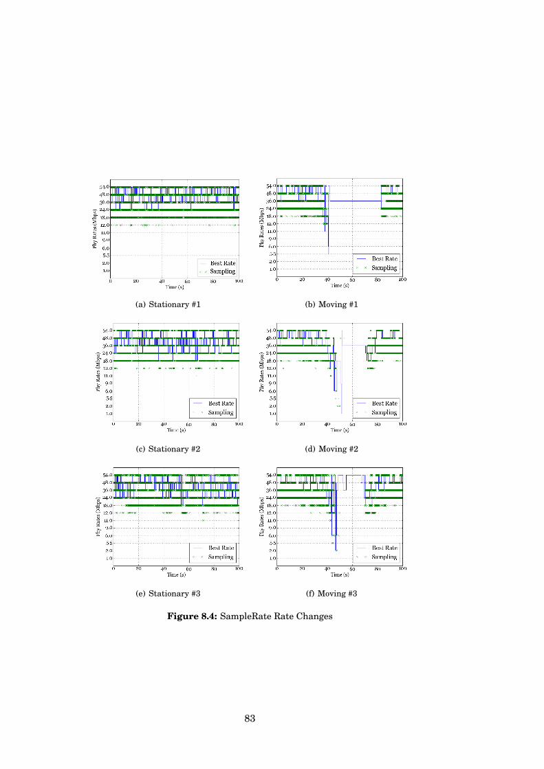
(a) Stationary #1 (b) Moving #1

(c) Stationary #2 (d) Moving #2

(e) Stationary #3 (f) Moving #3

Figure 8.4: SampleRate Rate Changes

83

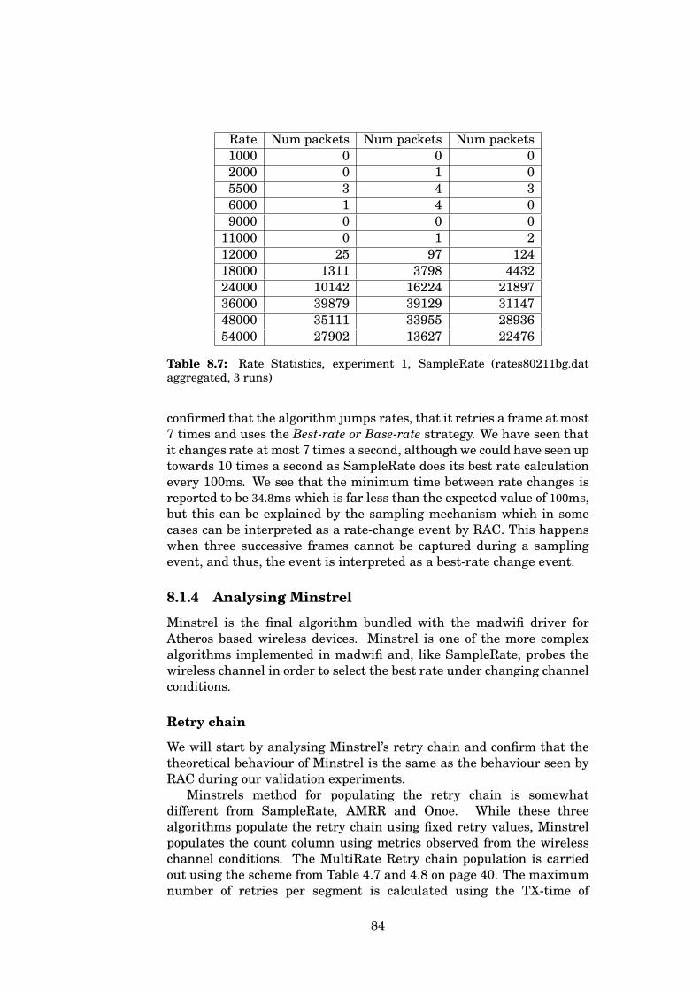
Rate Num packets Num packets Num packets1000 0 0 02000 0 1 05500 3 4 36000 1 4 09000 0 0 0

11000 0 1 212000 25 97 12418000 1311 3798 443224000 10142 16224 2189736000 39879 39129 3114748000 35111 33955 2893654000 27902 13627 22476

Table 8.7: Rate Statistics, experiment 1, SampleRate (rates80211bg.dataggregated, 3 runs)

confirmed that the algorithm jumps rates, that it retries a frame at most7 times and uses the Best-rate or Base-rate strategy. We have seen thatit changes rate at most 7 times a second, although we could have seen uptowards 10 times a second as SampleRate does its best rate calculationevery 100ms. We see that the minimum time between rate changes isreported to be 34.8ms which is far less than the expected value of 100ms,but this can be explained by the sampling mechanism which in somecases can be interpreted as a rate-change event by RAC. This happenswhen three successive frames cannot be captured during a samplingevent, and thus, the event is interpreted as a best-rate change event.

8.1.4 Analysing Minstrel

Minstrel is the final algorithm bundled with the madwifi driver forAtheros based wireless devices. Minstrel is one of the more complexalgorithms implemented in madwifi and, like SampleRate, probes thewireless channel in order to select the best rate under changing channelconditions.

Retry chain

We will start by analysing Minstrel’s retry chain and confirm that thetheoretical behaviour of Minstrel is the same as the behaviour seen byRAC during our validation experiments.

Minstrels method for populating the retry chain is somewhatdifferent from SampleRate, AMRR and Onoe. While these threealgorithms populate the retry chain using fixed retry values, Minstrelpopulates the count column using metrics observed from the wirelesschannel conditions. The MultiRate Retry chain population is carriedout using the scheme from Table 4.7 and 4.8 on page 40. The maximumnumber of retries per segment is calculated using the TX-time of

84

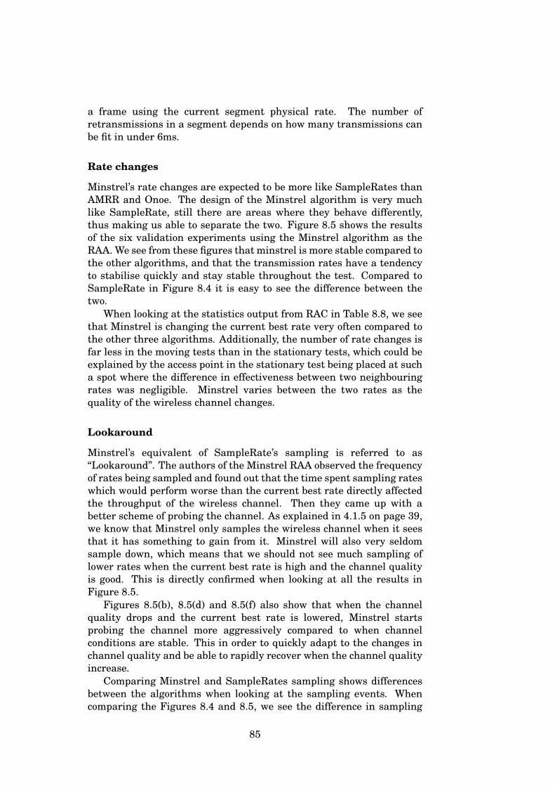
a frame using the current segment physical rate. The number ofretransmissions in a segment depends on how many transmissions canbe fit in under 6ms.

Rate changes

Minstrel’s rate changes are expected to be more like SampleRates thanAMRR and Onoe. The design of the Minstrel algorithm is very muchlike SampleRate, still there are areas where they behave differently,thus making us able to separate the two. Figure 8.5 shows the resultsof the six validation experiments using the Minstrel algorithm as theRAA. We see from these figures that minstrel is more stable compared tothe other algorithms, and that the transmission rates have a tendencyto stabilise quickly and stay stable throughout the test. Compared toSampleRate in Figure 8.4 it is easy to see the difference between thetwo.

When looking at the statistics output from RAC in Table 8.8, we seethat Minstrel is changing the current best rate very often compared tothe other three algorithms. Additionally, the number of rate changes isfar less in the moving tests than in the stationary tests, which could beexplained by the access point in the stationary test being placed at sucha spot where the difference in effectiveness between two neighbouringrates was negligible. Minstrel varies between the two rates as thequality of the wireless channel changes.

Lookaround

Minstrel’s equivalent of SampleRate’s sampling is referred to as“Lookaround”. The authors of the Minstrel RAA observed the frequencyof rates being sampled and found out that the time spent sampling rateswhich would perform worse than the current best rate directly affectedthe throughput of the wireless channel. Then they came up with abetter scheme of probing the channel. As explained in 4.1.5 on page 39,we know that Minstrel only samples the wireless channel when it seesthat it has something to gain from it. Minstrel will also very seldomsample down, which means that we should not see much sampling oflower rates when the current best rate is high and the channel qualityis good. This is directly confirmed when looking at all the results inFigure 8.5.

Figures 8.5(b), 8.5(d) and 8.5(f) also show that when the channelquality drops and the current best rate is lowered, Minstrel startsprobing the channel more aggressively compared to when channelconditions are stable. This in order to quickly adapt to the changes inchannel quality and be able to rapidly recover when the channel qualityincrease.

Comparing Minstrel and SampleRates sampling shows differencesbetween the algorithms when looking at the sampling events. Whencomparing the Figures 8.4 and 8.5, we see the difference in sampling

85

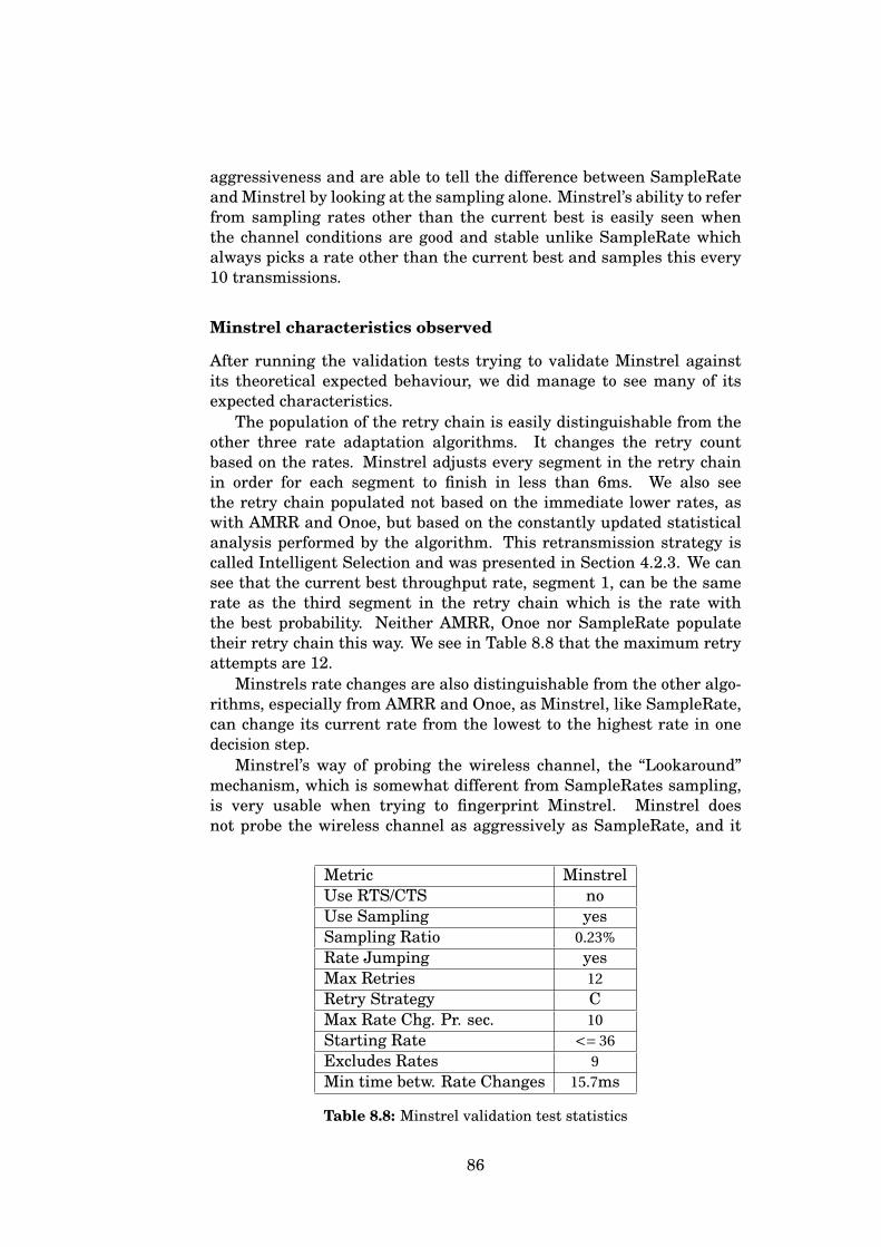
aggressiveness and are able to tell the difference between SampleRateand Minstrel by looking at the sampling alone. Minstrel’s ability to referfrom sampling rates other than the current best is easily seen whenthe channel conditions are good and stable unlike SampleRate whichalways picks a rate other than the current best and samples this every10 transmissions.

Minstrel characteristics observed

After running the validation tests trying to validate Minstrel againstits theoretical expected behaviour, we did manage to see many of itsexpected characteristics.

The population of the retry chain is easily distinguishable from theother three rate adaptation algorithms. It changes the retry countbased on the rates. Minstrel adjusts every segment in the retry chainin order for each segment to finish in less than 6ms. We also seethe retry chain populated not based on the immediate lower rates, aswith AMRR and Onoe, but based on the constantly updated statisticalanalysis performed by the algorithm. This retransmission strategy iscalled Intelligent Selection and was presented in Section 4.2.3. We cansee that the current best throughput rate, segment 1, can be the samerate as the third segment in the retry chain which is the rate withthe best probability. Neither AMRR, Onoe nor SampleRate populatetheir retry chain this way. We see in Table 8.8 that the maximum retryattempts are 12.

Minstrels rate changes are also distinguishable from the other algo-rithms, especially from AMRR and Onoe, as Minstrel, like SampleRate,can change its current rate from the lowest to the highest rate in onedecision step.

Minstrel’s way of probing the wireless channel, the “Lookaround”mechanism, which is somewhat different from SampleRates sampling,is very usable when trying to fingerprint Minstrel. Minstrel doesnot probe the wireless channel as aggressively as SampleRate, and it

Metric MinstrelUse RTS/CTS noUse Sampling yesSampling Ratio 0.23%Rate Jumping yesMax Retries 12Retry Strategy CMax Rate Chg. Pr. sec. 10Starting Rate <= 36Excludes Rates 9Min time betw. Rate Changes 15.7ms

Table 8.8: Minstrel validation test statistics

86

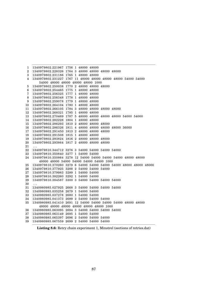
1 1340979802.221967 1756 1 48000 480002 1340979802.228326 1764 3 48000 48000 48000 480003 1340979802.231186 1765 1 48000 480004 1340979802.231227 1767 11 48000 48000 48000 48000 54000 54000

54000 48000 48000 48000 48000 10005 1340979802.250038 1770 2 48000 48000 480006 1340979802.254465 1775 1 48000 480007 1340979802.256325 1777 1 48000 480008 1340979802.256348 1778 1 48000 480009 1340979802.259078 1779 1 48000 48000

10 1340979802.264104 1780 1 48000 4800011 1340979802.266105 1784 3 48000 48000 48000 4800012 1340979802.268321 1785 1 48000 4800013 1340979802.270469 1787 5 48000 48000 48000 48000 54000 5400014 1340979802.282228 1804 1 48000 4800015 1340979802.286293 1810 2 48000 48000 4800016 1340979802.286326 1811 4 48000 48000 48000 48000 3600017 1340979802.291450 1813 2 48000 48000 4800018 1340979802.291508 1815 1 48000 4800019 1340979802.293824 1816 2 48000 48000 4800020 1340979802.293864 1817 2 48000 48000 4800021 . . .22 1340979810.344712 3276 3 54000 54000 54000 5400023 1340979810.350840 3277 1 54000 5400024 1340979810.350864 3278 12 54000 54000 54000 54000 48000 48000

48000 48000 54000 54000 54000 54000 100025 1340979810.370260 3279 6 54000 54000 54000 54000 48000 48000 4800026 1340979810.377925 3288 2 54000 54000 5400027 1340979810.379983 3289 1 54000 5400028 1340979810.382260 3292 1 54000 5400029 1340979810.384587 3300 3 54000 54000 54000 5400030 . . .31 1340980985.027925 2668 3 54000 54000 54000 5400032 1340980985.035258 2679 1 54000 5400033 1340980985.037278 2680 1 54000 5400034 1340980985.041373 2689 2 54000 54000 5400035 1340980985.041410 2691 12 54000 54000 54000 54000 48000 48000

48000 48000 48000 48000 48000 48000 100036 1340980985.063095 2694 3 54000 54000 54000 5400037 1340980985.063149 2695 1 54000 5400038 1340980985.065397 2696 2 54000 54000 5400039 1340980985.067559 2699 2 54000 54000 54000

Listing 8.6: Retry chain experiment 1, Minstrel (sections of retries.dat)

87

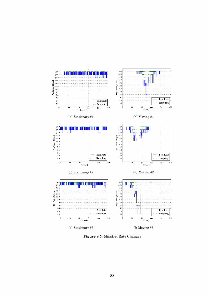
(a) Stationary #1 (b) Moving #1

(c) Stationary #2 (d) Moving #2

(e) Stationary #3 (f) Moving #3

Figure 8.5: Minstrel Rate Changes

88

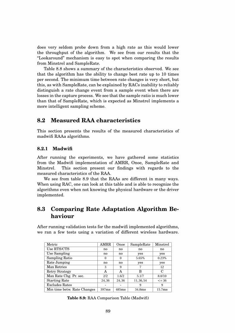
does very seldom probe down from a high rate as this would lowerthe throughput of the algorithm. We see from our results that the“Lookaround” mechanism is easy to spot when comparing the resultsfrom Minstrel and SampleRate.

Table 8.8 shows a summary of the characteristics observed. We seethat the algorithm has the ability to change best rate up to 10 timesper second. The minimum time between rate changes is very short, butthis, as with SampleRate, can be explained by RACs inability to reliablydistinguish a rate change event from a sample event when there arelosses in the capture process. We see that the sample ratio is much lowerthan that of SampleRate, which is expected as Minstrel implements amore intelligent sampling scheme.

8.2 Measured RAA characteristics

This section presents the results of the measured characteristics ofmadwifi RAAa algorithms.

8.2.1 Madwifi

After running the experiments, we have gathered some statisticsfrom the Madwifi implementation of AMRR, Onoe, SampleRate andMinstrel. This section present our findings with regards to themeasured characteristics of the RAA.

We see from table 8.9 that the RAAs are different in many ways.When using RAC, one can look at this table and is able to recognize thealgorithms even when not knowing the physical hardware or the driverimplemented.

8.3 Comparing Rate Adaptation Algorithm Be-haviour

After running validation tests for the madwifi implemented algorithms,we ran a few tests using a variation of different wireless hardware.

Metric AMRR Onoe SampleRate MinstrelUse RTS/CTS no no no noUse Sampling no no yes yesSampling Ratio 0 0 5.65% 0.23%Rate Jumping no no yes yesMax Retries 3 9 7 12Retry Strategy A A B CMax Rate Chg. Pr. sec. 2/2 1.6/2 5.1/7 8.0/10Starting Rate 24,36 24,36 11,36,54 <= 36Excludes Rates - - 9 9Min time betw. Rate Changes 397ms 485ms 34.8ms 15.7ms

Table 8.9: RAA Comparison Table (Madwifi)

89

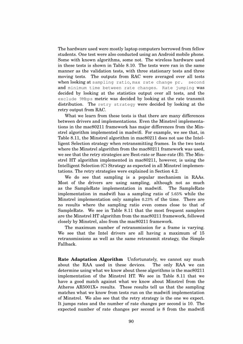
The hardware used were mostly laptop computers borrowed from fellowstudents. One test were also conducted using an Android mobile phone.Some with known algorithms, some not. The wireless hardware usedin these tests is shown in Table 8.10. The tests were ran in the samemanner as the validation tests, with three stationary tests and threemoving tests. The outputs from RAC were averaged over all testswhen looking at sampling ratio, max rate change pr. secondand minimum time between rate changes. Rate jumping wasdecided by looking at the statistics output over all tests, and theexclude 9Mbps metric was decided by looking at the rate transmitdistribution. The retry strategy were decided by looking at theretry output from RAC.

What we learn from these tests is that there are many differencesbetween drivers and implementations. Even the Minstrel implementa-tions in the mac80211 framework has major differences from the Min-strel algorithm implemented in madwifi. For example, we see that, inTable 8.11, the Minstrel algorithm in mac80211 does not use the Intel-ligent Selection strategy when retransmitting frames. In the two testswhere the Minstrel algorithm from the mac80211 framework was used,we see that the retry strategies are Best-rate or Base-rate (B). The Min-strel HT algorithm implemented in mac80211, however, is using theIntelligent Selection (C) Strategy as expected in all Minstrel implemen-tations. The retry strategies were explained in Section 4.2.

We do see that sampling is a popular mechanism in RAAs.Most of the drivers are using sampling, although not as muchas the SampleRate implementation in madwifi. The SampleRateimplementation in madwifi has a sampling ratio of 5.65% while theMinstrel implementation only samples 0.23% of the time. There areno results where the sampling ratio even comes close to that ofSampleRate. We see in Table 8.11 that the most frequent samplersare the Minstrel HT algorithm from the mac80211 framework, followedclosely by Minstrel, also from the mac80211 framework.

The maximum number of retransmission for a frame is varying.We see that the Intel drivers are all having a maximum of 15retransmissions as well as the same retransmit strategy, the SimpleFallback.

Rate Adaptation Algorithm Unfortunately, we cannot say muchabout the RAA used in these devices. The only RAA we candetermine using what we know about these algorithms is the mac80211implementation of the Minstrel HT. We see in Table 8.11 that wehave a good match against what we know about Minstrel from theAtheros AR5001X+ results. These results tell us that the samplingmatches what we know from tests run on the madwifi implementationof Minstrel. We also see that the retry strategy is the one we expect.It jumps rates and the number of rate changes per second is 10. Theexpected number of rate changes per second is 8 from the madwifi

90

implementation, but the source code of the mac80211 frameworkchanges this so the Minstrel implementation can change the best rateevery 100ms.

From the results shown in Table 8.11 we can conclude that none ofthe devices are running AMRR or Onoe because of the rate jumpingseen in all tests. Furthermore, we see that the sampling ratio is verylow which we know does not happen in SampleRate as well as we see theBroadcom BCM4318 [AirForce One 54g] devices use 9Mbps. The maxretry results tells us that neither AMRR nor Onoe are used, althoughboth SampleRate and Minstrel are likely candidates.

We can from this conclude that both SampleRate and Minstrel arelikely candidates for most if not all of the devices. Minstrel is inmost cases the most likely candidate, although the retry strategy is notalways the expected one.

91

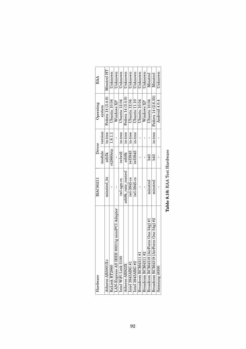
Har

dwar

eM

AC

8021

1D

rive

rO

pera

ting

RA

Am

odul

eve

rsio

nsy

stem

Ath

eros

AR

5001

X+

min

stre

l_ht

ath5

kin

-tre

eFe

dora

14(3

.4.0

)M

inst

relH

TR

aLin

kR

T28

60-

rt28

60st

a1.

8.1.

1U

bunt

u10

.04

Unk

now

nL

AN

-Exp

ress

AS

IEE

E80

211g

min

iPC

IA

dapt

er-

--

Win

dow

sX

PU

nkno

wn

Inte

lWiF

iLin

k51

00iw

l-ag

n-rs

iwlw

ifiin

-tre

eU

bunt

u12

.04

Unk

now

nA

ther

osA

R92

2Xat

h9k_

rate

_con

trol

ath9

kin

-tre

eFe

dora

14(3

.4.0

)U

nkno

wn

Inte

l394

5AB

G#1

iwl-

3945

-rs

iwl3

945

in-t

ree

Ubu

ntu

12.0

4U

nkno

wn

Inte

l394

5AB

G#2

iwl-

3945

-rs

iwl3

945

in-t

ree

Ubu

ntu

11.1

0U

nkno

wn

Bro

adco

mB

CM

4311

#1-

--

Ubu

ntu

10.0

4U

nkno

wn

Bro

adco

mB

CM

4311

#2-

--

Win

dow

sX

PU

nkno

wn

Bro

adco

mB

CM

4318

[Air

Forc

eO

ne54

g]#1

min

stre

lb4

3-

Ubu

ntu

10.0

4M

inst

rel

Bro

adco

mB

CM

4318

[Air

Forc

eO

ne54

g]#2

min

stre

lb4

3in

-tre

eFe

dora

14(2

.6.3

5)M

inst

rel

Sam

sung

i930

0-

--

And

roid

4.0.

4U

nkno

wn

Tabl

e8.

10:R

AA

Test

Har

dwar

e

92

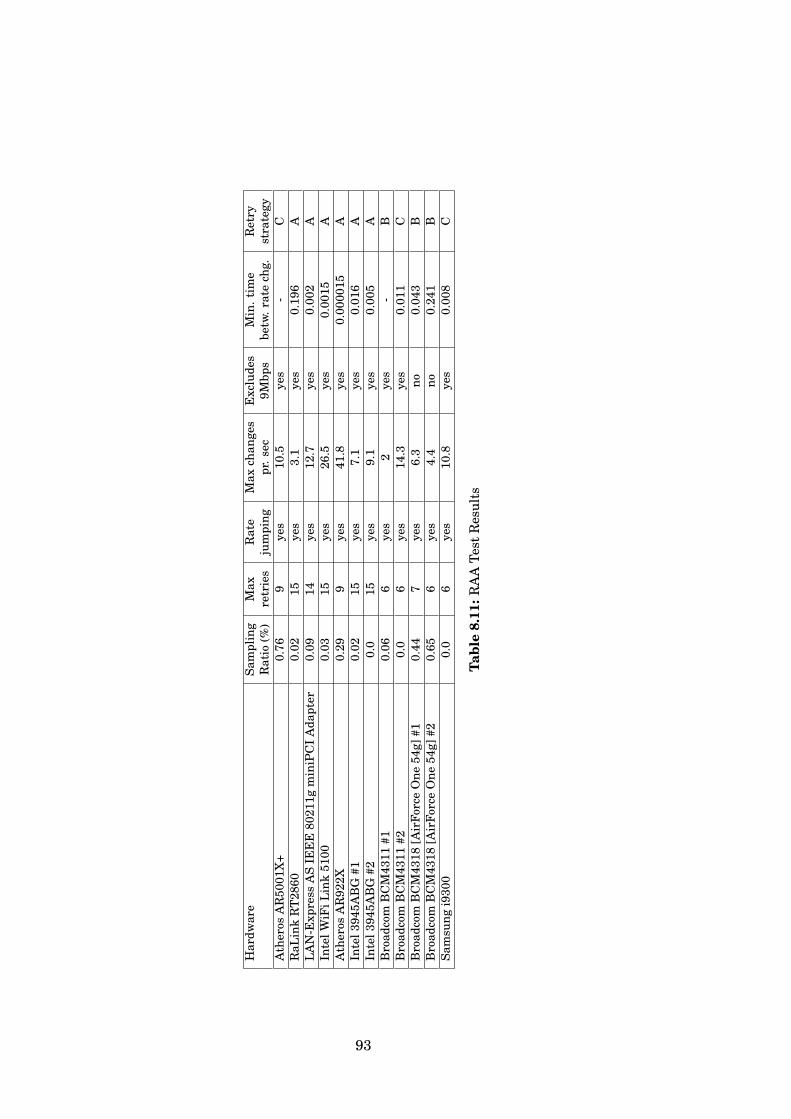
Har

dwar

eSa

mpl

ing

Max

Rat

eM

axch

ange

sE

xclu

des

Min

.tim

eR

etry

Rat

io(%

)re

trie

sju

mpi

ngpr

.sec

9Mbp

sbe

tw.r

ate

chg.

stra

tegy

Ath

eros

AR

5001

X+

0.76

9ye

s10

.5ye

s-

CR

aLin

kR

T28

600.

0215

yes

3.1

yes

0.19

6A

LA

N-E

xpre

ssA

SIE

EE

8021

1gm

iniP

CI

Ada

pter

0.09

14ye

s12

.7ye

s0.

002

AIn

telW

iFiL

ink

5100

0.03

15ye

s26

.5ye

s0.

0015

AA

ther

osA

R92

2X0.

299

yes

41.8

yes

0.00

0015

AIn

tel3

945A

BG

#10.

0215

yes

7.1

yes

0.01

6A

Inte

l394

5AB

G#2

0.0

15ye

s9.

1ye

s0.

005

AB

road

com

BC

M43

11#1

0.06

6ye

s2

yes

-B

Bro

adco

mB

CM

4311

#20.

06

yes

14.3

yes

0.01

1C

Bro

adco

mB

CM

4318

[Air

Forc

eO

ne54

g]#1

0.44

7ye

s6.

3no

0.04

3B

Bro

adco

mB

CM

4318

[Air

Forc

eO

ne54

g]#2

0.65

6ye

s4.

4no

0.24

1B

Sam

sung

i930

00.

06

yes

10.8

yes

0.00

8C

Tabl

e8.

11:R

AA

Test

Res

ults

93

Part VI

Conclusion and futurework

95

This thesis presented the Rate Adaptation Classifier (RAC) tooland a method to assist in classifying rate adaptation algorithms usedin IEEE 802.11 wireless network devices. The tool enables networkprofessionals and researchers to capture network traffic from specificdevices, enabling later analysis of the output for classifying the rateadaptation algorithm used. The RAAs present in the madwifi driveris AMRR, Onoe, SampleRate and Minstrel. There exists other RAAsin other drivers, but this thesis have focused on the ones present inmadwifi. The tool and accompanying method were successfully ableto detect algorithms used in the madwifi driver. We looked at otherdevices, but they did not show the behaviour of the madwifi RAAs.

The tool is capable of capturing and storing information whichenables us to distinguish different rate adaptation algorithms. Thisrequires there to be a classification process beforehand. Once a driverhas been classified and the metrics presented in this thesis have beendefined, the tool and accompanying method can be applied to determinethe rate adaptation method used.

The RAC tool and assisting method for determining RAAs werechosen because of the power it gives to the user. RAC may not be thebest solution in terms of flexibility, but the details it provides to the userabout the observed traffic is very precise.

We introduced retry strategy classifications: Simple Fallback, Best-rate or Base-rate and Intelligent Selection. We have seen that everydevice we have tested falls into one of these strategies.

A considerable amount of work was done researching and studyingthe RAAs implemented in the madwifi driver as well as the originaldesign and implementation of these algorithms. We have looked atother works trying to fingerprint RAAs using other methods, but wedecided that the manual method of RAC was most precise. We havestudied the IEEE 802.11 wireless network standard to be able toimplement the parsers required by RAC. Designing and implementingthe RAC tool with the accompanying method for determining RAAs wasdone incrementally throughout the thesis timespan. The RAC tool waswritten in C because of its speed and access to libraries such as libpcap.

The thesis presented experiments conducted to determine thecorrectness and effectiveness of RAC and accompanying method.Captured data from the RAC tool was compared to the captured datafrom Wireshark, and this did show that the capture engine of RAC isworking as expected. The RAC tool captures and interprets wirelessdata correctly. Experiments conducted on IEEE 802.11 hardwarerunning the madwifi driver did show that RAC and accompanyingmethod is able to determine the drivers RAA. Experiments whichwas run on wireless devices where the RAA was unknown or theimplementation was different than that of madwifi did show differentmetric values than the madwifi implementation. We could therefore notmap any of these algorithms to the ones implemented in the madwifidriver.

97

Future work

This thesis presented the statistics and results from experiments ranon four RAAs implemented in the madwifi driver: AMRR, Onoe,SampleRate and Minstrel. We did a comprehensive study on thebehaviour of these algorithms and presented the results from ourexperiments. We have seen that these implementations are recognizedby RAC and accompanying method. For this to work with otheralgorithms and implementations, there need to be a study of algorithmsand mapping the observed metric values for later use.

In the future, the RAC tool and accompanying method for classifyingRAAs can be merged together into one single tool. To accomplish this,the classification – and statistics engine of RAC has to be extended withknowledge on the behaviour of the different RAAs. RAC needs to beable to perform the mapping between the observed traffic patterns andthe defined metrics of an RAA. As of now, this process is performedmanually by the user.

98

Bibliography

[1] [Online]. http://www.radiotap.org, 07 2012.

[2] [Online]. http://www.linuxmanpages.com/man8/ifconfig.8.php, 07 2012.

[3] [Online]. http://www.tcpdump.org/, 07 2012.

[4] [Online]. http://www.wireshark.org/, 07 2012.

[5] P.A.K. Acharya, A. Sharma, E.M. Belding, K.C. Almeroth, andK. Papagiannaki. Rate adaptation in congested wireless networksthrough real-time measurements. Mobile Computing, IEEETransactions on, 9(11):1535 –1550, nov. 2010.

[6] R. Bruno, M. Conti, and E. Gregori. IEEE 802.11 optimalperformances: Rts/cts mechanism vs. basic access. In Personal,Indoor and Mobile Radio Communications, 2002. The 13th IEEEInternational Symposium on, volume 4, pages 1747 – 1751 vol.4,sept. 2002.

[7] O. Ekici and A. Yongacoglu. IEEE 802.11a throughput per-formance with hidden nodes. Communications Letters, IEEE,12(6):465 –467, june 2008.

[8] IEEE 802.11 Working Group. IEEE 802.11a-1999 - ofdm in the5ghz band, 1999.

[9] IEEE 802.11 Working Group. IEEE 802.11b-1999 - high rate dsssin the 2.4ghz band, 1999.

[10] IEEE 802.11 Working Group. IEEE 802.11g-2003 - further higherdata rate extension in the 2.4 ghz band, 2003.

[11] IEEE 802.11 Working Group. IEEE 802.11n-2009 - enhancementsfor higher throughput, 2009.

[12] Jianhua He, Wenyang Guan, Lin Bai, and Kai Chen. Theoreticanalysis of IEEE 802.11 rate adaptation algorithm samplerate.Communications Letters, IEEE, 15(5):524 –526, may 2011.

[13] Gavin Holland, Nitin Vaidya, and Paramvir Bahl. A rate-adaptivemac protocol for multi-hop wireless networks. In Proceedings of

99

the 7th annual international conference on Mobile computing andnetworking, MobiCom ’01, pages 236–251, New York, NY, USA,2001. ACM.

[14] “horst” project home page. [Online]. http://br1.einfach.org/tech/horst/, 07 2012.

[15] ISM. [Online]. http://en.wikipedia.org/wiki/ISM_band,07 2012.

[16] Ad Kamerman and Leo Monteban. WaveLAN(C)-II: a high-performance wireless LAN for the unlicensed band. Bell LabsTechnical Journal, 2(3):118–133, 1997.

[17] J. Kim, S. Kim, S. Choi, and D. Qiao. Cara: Collision-awarerate adaptation for IEEE 802.11 wlans. In INFOCOM 2006. 25thIEEE International Conference on Computer Communications.Proceedings, pages 1 –11, april 2006.

[18] Mathieu Lacage, Mohammad Hossein Manshaei, and ThierryTurletti. IEEE 802.11 rate adaptation: a practical approach. InProceedings of the 7th ACM international symposium on Modeling,analysis and simulation of wireless and mobile systems, MSWiM’04, pages 126–134, New York, NY, USA, 2004. ACM.

[19] About mac80211. [Online]. http://linuxwireless.org/en/developers/Documentation/mac80211, 07 2012.

[20] Ratul Mahajan, Maya Rodrig, David Wetherall, and John Zahor-jan. Analyzing the mac-level behavior of wireless networks inthe wild. In Proceedings of the 2006 conference on Applications,technologies, architectures, and protocols for computer communi-cations, SIGCOMM ’06, pages 75–86, New York, NY, USA, 2006.ACM.

[21] M. Mirza, P. Barford, Xiaojin Zhu, S. Banerjee, and M. Blodgett.Fingerprinting 802.11 rate adaption algorithms. In INFOCOM,2011 Proceedings IEEE, pages 1161 –1169, april 2011.

[22] Wireless Operating Modes. [Online]. http://wireless.kernel.org/en/users/Documentation/modes, 07 2012.

[23] Robert T. Morris, John C. Bicket, and John C. Bicket. Bit-rateselection in wireless networks. Technical report, Master’s thesis,MIT, 2005.

[24] Description of the Minstrel algorithm. [Online]. http://madwifi-project.org/browser/madwifi/branches/madwifi-0.9.4/ath_rate/minstrel/minstrel.txt, 072012.

100

[25] Description of the PID RAA algorithm. [Online]. http://linuxwireless.org/en/developers/Documentation/mac80211/RateControl/PID, 07 2012.

[26] Sourav Pal, Sumantra R. Kundu, Kalyan Basu, and Sajal K.Das. IEEE 802.11 rate control algorithms: Experimentation andperformance evaluation in infrastructure mode.

[27] Daji Qiao, Sunghyun Choi, Amit Jain, and Kang G. Shin. Miser: anoptimal low-energy transmission strategy for IEEE 802.11a/h. InProceedings of the 9th annual international conference on Mobilecomputing and networking, MobiCom ’03, pages 161–175, NewYork, NY, USA, 2003. ACM.

[28] U-NII. [Online]. http://en.wikipedia.org/wiki/U-NII, 072012.

[29] M. Vipin and S. Srikanth. Analysis of open source drivers for IEEE802.11 wlans. In Wireless Communication and Sensor Computing,2010. ICWCSC 2010. International Conference on, pages 1 –5, jan.2010.

101

Classifying Rate Adaptation Algorithms in IEEE … · Classifying Rate Adaptation Algorithms in...

Documents

Transcript of Classifying Rate Adaptation Algorithms in IEEE … · Classifying Rate Adaptation Algorithms in...