Important Notice

This copy may be used only for the purposes of research and

private study, and any use of the copy for a purpose other than research or private study may require the authorization of the copyright owner of the work in

question. Responsibility regarding questions of copyright that may arise in the use of this copy is

assumed by the recipient.

THE UNIVERSITY OF CALGARY

Fourier reconstruction of signal

by

Akshay Gulati

A DISSERTATION

SUBMITTED TO THE FACULTY OF GRADUATE STUDIES

IN PARTIAL FULFILLMENT OF THE REQUIREMENTS FOR THE

DEGREE OF MASTER OF SCIENCE

DEPARTMENT OF GEOSCIENCE

CALGARY, ALBERTA

May, 2011

c© Akshay Gulati 2011

THE UNIVERSITY OF CALGARY

FACULTY OF GRADUATE STUDIES

The undersigned certify that they have read, and recommend to the Faculty of Graduate

Studies for acceptance, a dissertation entitled “Fourier reconstruction of signal” submit-

ted by Akshay Gulati in partial fulfilment of the requirements for the degree of MASTER

OF SCIENCE.

Supervisor, Dr. Robert J FergusonDepartment of Geoscience

Dr. Larry LinesDepartment of Geoscience

Dr. Brian JackelDepartment of Physics and

Astronomy

Date

i

Abstract

This thesis addresses the problem of interpolating missing samples in seismic data. In-

terpolation is an important step in the seismic data processing flow, since most of the

pre-processing algorithms are designed to work with regularly sampled data.

In this thesis, I will focus on the Fourier reconstruction techniques which do not re-

quire a geological model as input, but use a priori information of the signal to reconstruct

the wavefield. This reconstruction requires that the signal be band limited.

Most presently available algorithms are slow, because of inability of fast Fourier

transform (FFT) to work with irregular samples. In case of the irregularity, the Dis-

crete Fourier transform (DFT) kernel is used for domain mapping. The computational

complexity of the DFT is O(N2) as compared to O(NlogN) for the FFT. This extra

computing time can cause processing delays so seismic data processors to use simple

regularization techniques which compromise accuracy for speed.

To address this problem, Non uniform Fast Fourier Transform (NFFT) is imple-

mented, which reduces the complexity of the DFT to O(NlogN) comparable to the

FFT. It has been used for seismic data regularization before using a Gaussian convolu-

tion kernel. Our newly proposed approach uses a Kaiser Bessel filter for convolution,

which gives a better result.

We applied this technique to solve the problem of clipped amplitudes in Ground

Penetrating Radar data. The NFFT is hybridized with the POCS (Projection on Convex

Sets) method to restore clipped peaks from an acquired GPR data set.

ii

Acknowledgements

I would like to thank my supervisor Dr. Rob Ferguson for his excellent support through-

out my program, and providing me with so many inspiring ideas. I am very grateful to

Dr. Daniel Potts and Dr. Stefan Kunis for their NFFT software package. My sincere

thanks go to all of my colleagues at the University of Calgary, especially to Marcus Wilson

who eased the understanding of complex Mathmatical analysis and to Kevin Hall who

always had to solve my computer problems. A special thanks to Dr. Mostafa Naghizadeh

for his guidance in understanding the concept of the Fourier reconstruction. I can’t say

enough thanks to my friend Ritesh Kumar Sharma who stood by my side throughout the

program and also made my shift to geophysics a smooth one. My gratitude to my friend

Anshita for her support, and for cooking me the best meals I ever had during college life.

Above all, I want to express my most cordial gratitude to my parents for their love and

support over the years.

iii

DEDICATIONS

To my father, Sailesh Gulati and my mother, Savita Gulati.

iv

Table of Contents

Approval Page . . . . . . . . . . . . . . . . . . . . . . . . . . . . . . . . . . . iAbstract . . . . . . . . . . . . . . . . . . . . . . . . . . . . . . . . . . . . . . . iiAcknowledgements . . . . . . . . . . . . . . . . . . . . . . . . . . . . . . . . . iiiTable of Contents . . . . . . . . . . . . . . . . . . . . . . . . . . . . . . . . . . vList of Figures . . . . . . . . . . . . . . . . . . . . . . . . . . . . . . . . . . . . vii1 Introduction . . . . . . . . . . . . . . . . . . . . . . . . . . . . . . . . . . 11.1 The need for Interpolation . . . . . . . . . . . . . . . . . . . . . . . . . . 11.2 Reviews of Seismic data Reconstruction Methods . . . . . . . . . . . . . 2

1.2.1 Factor affecting Seismic Data Reconstruction . . . . . . . . . . . . 41.2.2 Motivations . . . . . . . . . . . . . . . . . . . . . . . . . . . . . . 51.2.3 Contribution . . . . . . . . . . . . . . . . . . . . . . . . . . . . . 61.2.4 Organization of this thesis . . . . . . . . . . . . . . . . . . . . . . 6

2 Band limited signal reconstruction . . . . . . . . . . . . . . . . . . . . . . 82.1 Summary . . . . . . . . . . . . . . . . . . . . . . . . . . . . . . . . . . . 82.2 Introduction . . . . . . . . . . . . . . . . . . . . . . . . . . . . . . . . . . 82.3 Theory . . . . . . . . . . . . . . . . . . . . . . . . . . . . . . . . . . . . . 9

2.3.1 ACT Method . . . . . . . . . . . . . . . . . . . . . . . . . . . . . 92.4 Examples . . . . . . . . . . . . . . . . . . . . . . . . . . . . . . . . . . . 10

2.4.1 Uniform Decimation . . . . . . . . . . . . . . . . . . . . . . . . . 112.4.2 Random Decimation . . . . . . . . . . . . . . . . . . . . . . . . . 11

2.5 Conclusion . . . . . . . . . . . . . . . . . . . . . . . . . . . . . . . . . . . 143 Kaiser Bessel gridding kernel for seismic data regularization . . . . . . . 213.1 Summary . . . . . . . . . . . . . . . . . . . . . . . . . . . . . . . . . . . 213.2 Introduction . . . . . . . . . . . . . . . . . . . . . . . . . . . . . . . . . . 213.3 Theory . . . . . . . . . . . . . . . . . . . . . . . . . . . . . . . . . . . . . 22

3.3.1 Discrete Fourier Transform . . . . . . . . . . . . . . . . . . . . . . 233.4 Methodology . . . . . . . . . . . . . . . . . . . . . . . . . . . . . . . . . 27

3.4.1 Forward problem . . . . . . . . . . . . . . . . . . . . . . . . . . . 273.4.2 Window function . . . . . . . . . . . . . . . . . . . . . . . . . . . 293.4.3 Comparision . . . . . . . . . . . . . . . . . . . . . . . . . . . . . . 313.4.4 Inversion . . . . . . . . . . . . . . . . . . . . . . . . . . . . . . . . 34

3.5 Efficiency . . . . . . . . . . . . . . . . . . . . . . . . . . . . . . . . . . . 343.6 Synthetic Tests . . . . . . . . . . . . . . . . . . . . . . . . . . . . . . . . 35

3.6.1 Synthetic 1D examples . . . . . . . . . . . . . . . . . . . . . . . . 353.6.2 Gaps . . . . . . . . . . . . . . . . . . . . . . . . . . . . . . . . . . 383.6.3 Extrapolation . . . . . . . . . . . . . . . . . . . . . . . . . . . . . 40

3.7 Synthetic 2D examples . . . . . . . . . . . . . . . . . . . . . . . . . . . . 403.7.1 Randomly decimated dipping Events . . . . . . . . . . . . . . . . 403.7.2 Uniform decimation for dipping events . . . . . . . . . . . . . . . 433.7.3 Hyperbolic events . . . . . . . . . . . . . . . . . . . . . . . . . . . 45

3.8 Conclusion . . . . . . . . . . . . . . . . . . . . . . . . . . . . . . . . . . . 45

v

4 A simple algorithm for the restoration of clipped GPR amplitudes . . . . 494.1 summary . . . . . . . . . . . . . . . . . . . . . . . . . . . . . . . . . . . . 494.2 Introduction . . . . . . . . . . . . . . . . . . . . . . . . . . . . . . . . . . 49

4.2.1 Theory . . . . . . . . . . . . . . . . . . . . . . . . . . . . . . . . . 524.3 Experiment . . . . . . . . . . . . . . . . . . . . . . . . . . . . . . . . . . 55

4.3.1 Synthetic data . . . . . . . . . . . . . . . . . . . . . . . . . . . . . 554.3.2 Real data . . . . . . . . . . . . . . . . . . . . . . . . . . . . . . . 58

4.4 Conclusion . . . . . . . . . . . . . . . . . . . . . . . . . . . . . . . . . . . 715 Conclusion . . . . . . . . . . . . . . . . . . . . . . . . . . . . . . . . . . . 72

vi

List of Figures

2.1 (a) A simple harmonic and a uniform 50% decimation of that harmonic. (b) The original signal2.2 (a) A stationary seismic trace and a uniform 50% decimation of that trace. (b) The original2.3 (a) A simple harmonic and a random 40% decimation of that harmonic. (b) The original signal2.4 (a) A simple harmonic and a random 70% decimation of that harmonic. (b) The original signal2.5 (a) A simple harmonic and a random 70% decimation of that harmonic. (b) The original signal2.6 (a) A simple harmonic and a random 70% decimation of that harmonic. (b) The original signal2.7 (a) A stationary seismic trace and a random 30% decimation of that trace. (b) The original2.8 (a) A stationary seismic trace and a random 50% decimation of that trace. (b) The original

3.1 Kaiser Bessel filter. a) Kaiser window in spatial domain. b) Kaiser window in Fourier domain.3.2 RMS error vs number of iterations and percent decimation for Gaussian window 323.3 RMS error vs number of iterations and percent decimation for Kaiser Bessel window 333.4 Effect of sampling on seismic data. a) Hyperbolic events in spatial domain. b) Fourier domain3.5 Reconstruction for Harmonics. a) Harmonics with 30 % decimation. b) Harmonics with 503.6 Reconstruction and extrapolation of gaps. a) Small size gaps. b) Reconstructed small gapp3.7 Synthetic seismic data. a) Synthetic original data. b) Missing traces section with 10 % decimation.3.8 Fourier domain representation. a) Fourier domain for original data. b) Fourier domain for missing3.9 Reconstruction of random sampled heismic data. a) 50 % Decimated data. b) Reconstructed3.10 Reconstruction of uniformly sampled seismic data. a) Decimation by factor of 2. b) Reconstructed3.11 Reconstruction of hyperbolic events. a) Hyperbolic events with 20 % uniform decimation. b)

4.1 Ground penetrating radar (GPR) uses radio waves to probe the subsurface of lossy dielectric4.2 The principle of POCS Method . . . . . . . . . . . . . . . . . . . . . . . 534.3 flowchart . . . . . . . . . . . . . . . . . . . . . . . . . . . . . . . . . . . . 544.4 Synthetic sections. a) Original synthetic data. b) Clipped data. c) Reconstructed data. 564.5 a) Synthetic trace. b) Clipped trace. c) Reconstructed trace . . . . . . . 574.6 Acquired GPR data with clipped horizons. . . . . . . . . . . . . . . . . . 594.7 Random extracted clipped trace from acquired GPR data. . . . . . . . . 604.8 Comparative study for reconstruction of clipped amplitude . . . . . . . . 614.9 Spline interpolation of clipped GPR data. . . . . . . . . . . . . . . . . . 624.10 Restored clipped amplitudes using Spline and Hybrid NFFT POCS. a) 10th trace from restored4.11 Restored clipped amplitudes using Spline and Hybrid NFFT POCS. a) 100th trace from restored4.12 Restored clipped amplitudes using Spline and Hybrid NFFT POCS. a) 250th trace from restored4.13 Reconstructed data using Hybrid NFFT-POCS . . . . . . . . . . . . . . 674.14 Residual between original and reconstructed section using Hybrid NFFT-POCS. 684.15 Residual between original and reconstructed section using spline interpolation. 694.16 Residual between restored GPR section using spline and Hybird NFFT-POCS. 70

vii

Chapter 1

Introduction

The objective of any processing method is to refine the image of the subsurface obtained

during acquisition. In exploration geophysics, our goal is to acquire, process and invert

seismic wavefields to explore the potential hydrocarbons among the complex structures

underneath the earth. In these methods, a seismic energy source, generally generated by

an explosion, vibroseis truck or air gun travels through the earth’s crust. Discontinuities

in the earth’s composition cause this energy to reflect and travel back to the surface. The

travel time of this energy captured by an array of geophones. This gathered information

is processed to improve the signal to noise ratio enhancement and finally, used to define

an image of subsurface via inversion algorithms. The image produced in the end is used as

a initial platform for the geophysical interpretation for exploring the geological structure,

sedimentological models and process that in applied seismology can be use to delineate

and exploit accumulation of hydrocarbons.

1.1 The need for Interpolation

Regular sampling is one of the major concerns during acquisition of seismic data. The

process of acquisition prefers to record a regular finite number of spatial samples of the

continuous wavefield. Regular distribution of sources and receivers leads to a better

quality image. But, in the field actual sampling of seismic data is generally far from this

ideal condition. In difficult terrain, due to manual error or some technical irregularity it

is possible to have missing and corrupted traces in the data. Ignoring this irregularities

can result in a distorted subsurface image. This irregular sampling is a major burden on

1

many data processing algorithms, including wave equation migration and many multiple

removal method’s which require regularly and densely sampled data as input.

During seismic data acquisition, the continuous wavefield is sampled as a discrete

wave field based on the grid of survey. For reconstruction of the continuous wave field

acquisition geometry i:e for mapping the irregular data on the regular grid, sampling

rate for any axis must be equal or greater than twice dominant frequency of continuous

signal (Unser, 2000). The source and receiver interval’s should be decided based on

the Nyquist rule (Vermeer, 1990). When this rule is neglected, interpolation comes in

to play to reconstruct the data to a populated distribution of source and receivers and

reproduce an approximation of the original survey (Liu and Sacchi, 2004). The quality of

the reconstructed data directly affects the various steps of processing such as Migration

(Spitz, 1991), AVO analysis (Sacchi and Liu, 2005), imaging (Liu and Sacchi, 2004) and

noise removal

(Abma and Kabir, 2005) (Soubaras, 1994).

1.2 Reviews of Seismic data Reconstruction Methods

Seismic data reconstruction methods are all related in the sense that they are tasked with

restoring the spatial continuity of wavefield (Naghizadeh and Sacchi, 2010). Seismic data

reconstruction algorithms are divided in to two categories: those based on wave equation

analysis and those based on parametric analysis.

Wave equation based methods work using a regression approach, using the physics

of wave propagation to reconstruct the missing samples. In geophysics, numerous ap-

proaches based on this model are proposed (Ronen, 1987; Bagaini and Spagnolini, 1999;

Stolt, 2002; Trad, 2003; Fomel, 2003). Wave equation based methods require a priori

knowledge of velocity model as input.

2

Parametric analysis based reconstruction methods are based on the a priori infor-

mation from the seismic data alone (Naghizadeh and Sacchi, 2009a). Most parametric

reconstruction methods are based on Fourier transformation from one domain to another

(Naghizadeh and Sacchi, 2008b,c, 2009b). In the last few years excellent research is been

done in this area (Liu and Sacchi, 2004; Schonewille et al., 2009). The prior assumption

is either based on the stationarity of the process or based on the fact that most of the

power in the power spectrum is concentrated on the lower frequencies, analysis based on

this fact known as bandlimitness (Naghizadeh and Sacchi, 2010). Bandlimitness enforces

only the use of certain set of frequencies (Feichtinger et al., 1995b). These algorithms

perform efficiently even in situations where bandlimited assumption is not satisfied ex-

actly (Trad, 2008).

Seismic data reconstruction is based on data mapping, generally mapping of spatial

domain data to the Fourier domain. The most common bases for obtaining high resolu-

tion reconstruction techniques are the Fourier transform (Sacchi et al., 1998; Xu et al.,

2005; Liu and Sacchi, 2004; Naghizadeh and Sacchi, 2007b, 2008a, 2009b, 2007a) and the

Radon transform (Darche, 1990; Verschuur and Kabir, 1995). In the parabolic Radon

transform, two CMP (Common Mid Point)gathers are combined to improve offset sam-

pling and thus differences between midpoint positions are ignored (Duijndam et al.,

1999). Similarly hyperbolic and linear Radon transforms (Thorson and Claerbout, 1985)

as well as the parabolic Radon transform are suitable for estimating frequencies at irregu-

lar nodes, but they suffer aliasing problem due to sparse sampling (Hugonnet and Canadas,

1995), the local Radon transform and the curvelet transform (Hennenfent and Herrmann,

2006b, 2007, 2006a). Another group of signal processing interpolation methods rely on

prediction error filtering techniques (Wiggins and Miller, 1972; Spitz, 1991) and (Porsani,

1999) introduced seismic trace interpolation methods using prediction filters. These

methods operate frequency-space (f-x ) domain. The low frequencies in a regular spa-

3

tial grid are used to estimate the prediction filters needed to interpolate high frequency

components. This regular spatial grid requirement restrict prediction filter methods to

regular sampling.

1.2.1 Factor affecting Seismic Data Reconstruction

It is important to identify the factors which can affect the reconstruction technique. In

my thesis, I check the effectiveness of given methods by using them on various conditions.

These conditions are created by use of one or more factors given below

1. Sampling: The sampling operator has a significant impact on the reconstruction

of seismic data. The sampling operator is a function which can be applied to

regular data to model trace decimation. Regularization can be thought of as the

inverse of this operator. Regular sampling function results in a regular but more

sparsely sampled seismic data set and an irregular sampling function is responsible

for a randomly sampled data set. The interpolation techniques work differently

for the regular and irregular seismic data. Currently available techniques generally

prefer regular sampling to irregular sampling. However new techniques based on

the theory of compressed sensing recovered the data on the basis of superposition

of a small number of basis functions.

2. Aliasing : The aliasing plays a major role in determining the effectiveness of an

algorithm. Aliasing results in the duplication of events. Lower aliasing is easy

to remove and reconstructing the missing sample. But, in case of highly aliased

events, most of the algorithms fails (Naghizadeh and Sacchi, 2007b, 2008a, 2009b,

2007a). On, the basis of this many researchers advocate irregular sampling to avoid

aliasing.

4

3. Decimation factor: Seismic reconstruction algorithms cannot be expected to

succeed on every input. Each algorithm has its own maximum decimation factor,

above which the algorithm will start fail. Thus it is important to test the limitations

of each algorithm.

4. Dimension of data : Fourier methods can always be extended to higher dimen-

sions. Methods which make use of all dimensions of the data, perform better. This

is due to the fact that if one spatial dimension is poorly sampled, then the other

dimensions algorithm can be used to reconstruct the missing samples. In this thesis

algorithms are tested on just one dimension, and can be extended simply to several

dimension.

5. Event orientation: Reconstruction algorithm produce satisfactory results when

tested on seismic data with low dips. Events with high dips are always the one

difficult to recover (Naghizadeh and Sacchi, 2008a, 2009b). It is important for

the algorithm to be tested on steeply dipping events. For curved events, Spatial

windowing is always recommend. Spatial windowing will approximate curved events

as locally linear events.

1.2.2 Motivations

The main motivation of this thesis is to introduce Fast Fourier reconstruction techniques

that can be used for seismic data reconstruction. The objective is to provide reconstruc-

tion method that can:

• be used to reconstruct regular as well as irregular seismic data.

• speed up presently available Fourier reconstruction techniques.

• handle aliased energy.

5

1.2.3 Contribution

The main contribution of this thesis are:

• The introduction of a new fast kernel for seismic data regularization.

• The hybrid approach using this kernel for declipping acquired GPR data.

1.2.4 Organization of this thesis

This thesis is organized as follows:

• Chapter 2 presents the popular Adaptive weights Conjugate gradient Toeplitz

(ACT) algorithm for signal construction. This algorithm is slow but accurate, and

validated on several typical trace regularization situations.

• Chapter 3 introduces the faster version of ACT, we introduced the Kaiser Bessel

Non uniform Fast Fourier transform kernel (NFFT). The Kaiser Bessel NFFT kernel

balances accuracy and computational cost, and we present an application of this

NFFT for seismic trace interpolation. Application of the Bessel kernel for non-

uniform samples is not a new algorithm, but it is an approximation scheme that can

be used to calculate an approximate spectrum. In one dimension, the computational

complexity of Kaiser Bessel NFFT is O(NlogN) which is a dramatic improvement

from the O(N2) complexity of the DFT use by ACT, and it is comparable to the

FFT. This algorithm can be easily extended to higher dimensions. Least squares

is used to refine an approximated Fourier spectrum followed by simple Inverse Fast

Fourier transform (IFFT). The applicability of the proposed method is examined

using synthetic seismic data.

• Chapter 4 deals with the common problem of clipped data encountered during

GPR acquisition. The Kaiser Bessel NFFT with well known POCS (Projection

6

on convex set) is applied. This hybrid approach is been tested on synthetic data,

finally leading to some real GPR data set processing.

• Chapter 5 concludes the thesis with summary of results.

7

Chapter 2

Band limited signal reconstruction

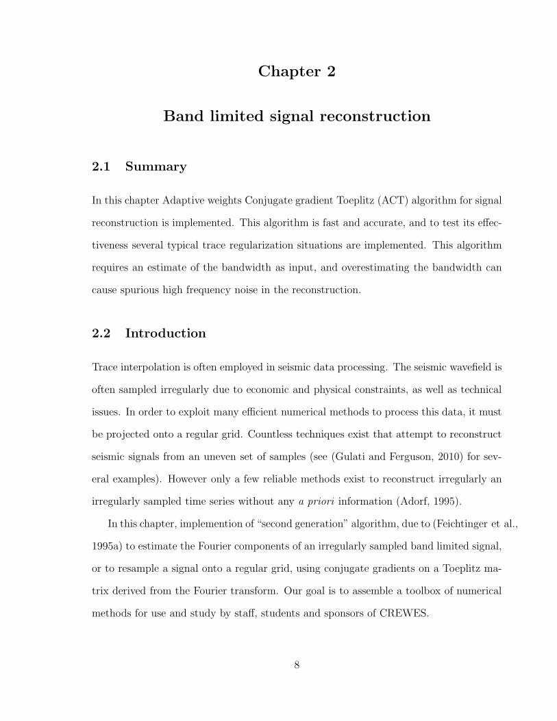
2.1 Summary

In this chapter Adaptive weights Conjugate gradient Toeplitz (ACT) algorithm for signal

reconstruction is implemented. This algorithm is fast and accurate, and to test its effec-

tiveness several typical trace regularization situations are implemented. This algorithm

requires an estimate of the bandwidth as input, and overestimating the bandwidth can

cause spurious high frequency noise in the reconstruction.

2.2 Introduction

Trace interpolation is often employed in seismic data processing. The seismic wavefield is

often sampled irregularly due to economic and physical constraints, as well as technical

issues. In order to exploit many efficient numerical methods to process this data, it must

be projected onto a regular grid. Countless techniques exist that attempt to reconstruct

seismic signals from an uneven set of samples (see (Gulati and Ferguson, 2010) for sev-

eral examples). However only a few reliable methods exist to reconstruct irregularly an

irregularly sampled time series without any a priori information (Adorf, 1995).

In this chapter, implemention of “second generation” algorithm, due to (Feichtinger et al.,

1995a) to estimate the Fourier components of an irregularly sampled band limited signal,

or to resample a signal onto a regular grid, using conjugate gradients on a Toeplitz ma-

trix derived from the Fourier transform. Our goal is to assemble a toolbox of numerical

methods for use and study by staff, students and sponsors of CREWES.

8

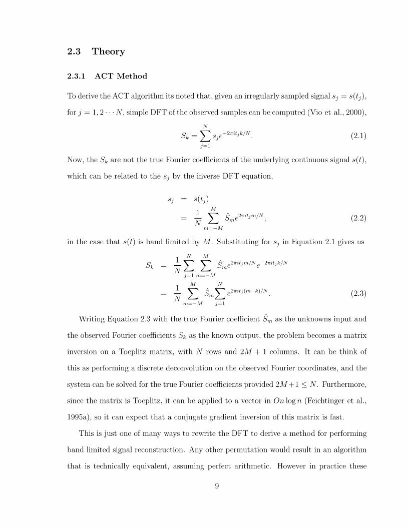
2.3 Theory

2.3.1 ACT Method

To derive the ACT algorithm its noted that, given an irregularly sampled signal sj = s(tj),

for j = 1, 2 · · ·N , simple DFT of the observed samples can be computed (Vio et al., 2000),

Sk =N∑

j=1

sje−2πitjk/N . (2.1)

Now, the Sk are not the true Fourier coefficients of the underlying continuous signal s(t),

which can be related to the sj by the inverse DFT equation,

sj = s(tj)

=1

N

M∑

m=−M

Sme2πitjm/N , (2.2)

in the case that s(t) is band limited by M . Substituting for sj in Equation 2.1 gives us

Sk =1

N

N∑

j=1

M∑

m=−M

Sme2πitjm/Ne−2πitjk/N

=1

N

M∑

m=−M

Sm

N∑

j=1

e2πitj (m−k)/N . (2.3)

Writing Equation 2.3 with the true Fourier coefficient Sm as the unknowns input and

the observed Fourier coefficients Sk as the known output, the problem becomes a matrix

inversion on a Toeplitz matrix, with N rows and 2M + 1 columns. It can be think of

this as performing a discrete deconvolution on the observed Fourier coordinates, and the

system can be solved for the true Fourier coefficients provided 2M+1 ≤ N . Furthermore,

since the matrix is Toeplitz, it can be applied to a vector in On logn (Feichtinger et al.,

1995a), so it can expect that a conjugate gradient inversion of this matrix is fast.

This is just one of many ways to rewrite the DFT to derive a method for performing

band limited signal reconstruction. Any other permutation would result in an algorithm

that is technically equivalent, assuming perfect arithmetic. However in practice these

9

methods will have different properties and one can be more effective than another in

certain situations (Vio et al., 2000).

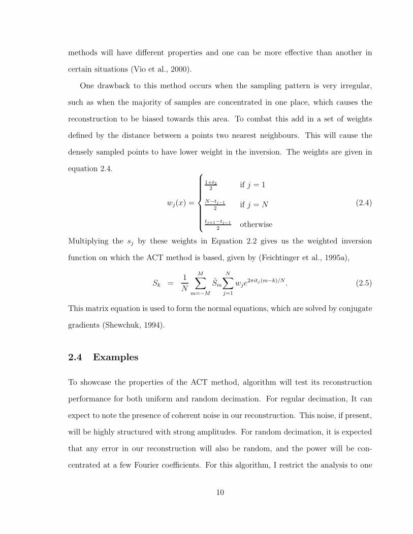
One drawback to this method occurs when the sampling pattern is very irregular,

such as when the majority of samples are concentrated in one place, which causes the

reconstruction to be biased towards this area. To combat this add in a set of weights

defined by the distance between a points two nearest neighbours. This will cause the

densely sampled points to have lower weight in the inversion. The weights are given in

equation 2.4.

wj(x) =

1+t22

if j = 1

N−tj−1

2if j = N

tj+1−tj−1

2otherwise

(2.4)

Multiplying the sj by these weights in Equation 2.2 gives us the weighted inversion

function on which the ACT method is based, given by (Feichtinger et al., 1995a),

Sk =1

N

M∑

m=−M

Sm

N∑

j=1

wje2πitj (m−k)/N . (2.5)

This matrix equation is used to form the normal equations, which are solved by conjugate

gradients (Shewchuk, 1994).

2.4 Examples

To showcase the properties of the ACT method, algorithm will test its reconstruction

performance for both uniform and random decimation. For regular decimation, It can

expect to note the presence of coherent noise in our reconstruction. This noise, if present,

will be highly structured with strong amplitudes. For random decimation, it is expected

that any error in our reconstruction will also be random, and the power will be con-

centrated at a few Fourier coefficients. For this algorithm, I restrict the analysis to one

10

dimensional signals, where the problem can be thought of as the reconstruction of a time

series.

2.4.1 Uniform Decimation

Figure 2.1a shows a simple signal composed of two superimposed harmonics. The top

panel shows the true signal, and the lower panel shows a uniform sampling of 50% of

the signal. Figure 2.1b shows the discrete Fourier transform of the decimated signal.

Note that the distortion of the spectrum is highly structured with high amplitude aliases.

Inserting zeros into the signal to denote the missing traces results in the Fourier spectrum

in Figure 2.1e. Note that the spectrum is the same but with more detail. Figure 2.1b

shows the reconstructed harmonic after two iterations, and Figure 2.1d shows the Fourier

spectrum. The ACT method converges linearly in relative error to the solution in the

case of uniform decimation, and this simple signal is perfectly reconstructed.

The top of Figure 2.2a shows a seismic signal composed of 650 samples from a 25Hz

Ricker wavelet convolved with a random reflectivity series, and the bottom panel shows

the same signal with 50% of the samples set to zero. Figure 2.2b shows the reconstruction

of the signal in the time domain. The reconstructed signal agrees quite well with the

original signal. As with the last example, the ACT method linearly converges to the

solution (Figure 2.2c), so it is very effective for uniform decimation.

2.4.2 Random Decimation

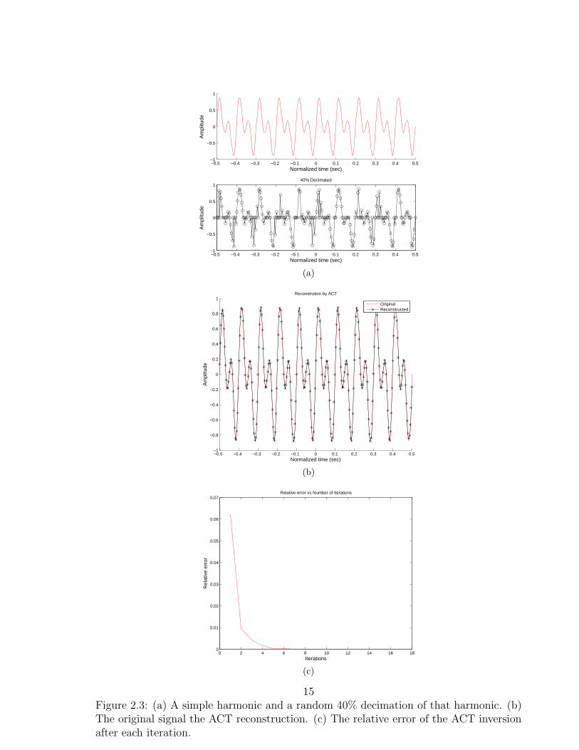
Figure 2.3a shows the same harmonic, but with a random selection of 40% amplitudes

values set to zero. Figure 2.3b shows the reconstructed harmonic, which agrees with

the original almost everywhere. Figure 2.3c shows that the relative error of the solution

decays exponentially with the number of iterations. This is less desirable than the linear

convergence, its been noted in the uniform decimation examples. Figures 2.4, 2.5, and

11

−0.5 −0.4 −0.3 −0.2 −0.1 0 0.1 0.2 0.3 0.4 0.5−1

−0.5

0

0.5

1

−0.5 −0.4 −0.3 −0.2 −0.1 0 0.1 0.2 0.3 0.4 0.5−1

−0.5

0

0.5

1

Normalized time (sec)

Am

plitu

de

50% Decimtaed

(a)

−0.5 −0.4 −0.3 −0.2 −0.1 0 0.1 0.2 0.3 0.4 0.5−1

−0.8

−0.6

−0.4

−0.2

0

0.2

0.4

0.6

0.8

1

Normalized time (sec)

Am

plitu

de

Reconstrution by ACT

OriginalReconstructed

(b)

0 20 40 60 80 100 120 1400

0.1

0.2

0.3

0.4

0.5

0.6

0.7

0.8

0.9

freq (Hz)

Am

plitu

de

(c)

0 10 20 30 40 50 60 700

10

20

30

40

50

60

70

freq (Hz)

Am

plitu

de

(d)

0 50 100 150 200 250 3000

0.1

0.2

0.3

0.4

0.5

0.6

0.7

0.8

0.9

freq (Hz)

Am

plitu

de

(e)

1 1.5 2 2.5 3 3.5 40

0.01

0.02

0.03

0.04

0.05

0.06

0.07

Iterations

Rel

ativ

e er

ror

Relative error vs Number of Iterations

(f)

Figure 2.1: (a) A simple harmonic and a uniform 50% decimation of that harmonic.(b) The original signal and the ACT reconstruction. (c) The Fourier spectrum of thedecimated signal. (d) The Fourier spectrum of the reconstructed signal. (e) The Fourierspectrum of the decimated signal with zeros in place of the unknown samples. (f) Therelative error of the ACT inversion after each iteration.12

−0.5 −0.4 −0.3 −0.2 −0.1 0 0.1 0.2 0.3 0.4 0.5−0.15

−0.1

−0.05

0

0.05

0.1

Normalized time (sec)

Am

plitu

de

Original Trace

−0.5 −0.4 −0.3 −0.2 −0.1 0 0.1 0.2 0.3 0.4 0.5−0.1

−0.05

0

0.05

0.1

Normalized time (sec)

Am

plitu

de

Decimated by factor of 2

(a)

−0.5 −0.4 −0.3 −0.2 −0.1 0 0.1 0.2 0.3 0.4 0.5−0.15

−0.1

−0.05

0

0.05

0.1

Normalized time(sec)

Am

plitu

de

Reconstrution by ACT

OriginalReconstructed

(b)

1 1.5 2 2.5 3 3.5 4 4.5 50

0.005

0.01

0.015

0.02

0.025

0.03

0.035

0.04

Iterations →

Rel

ativ

e er

ror

Relative error vs Number of Iterations

(c)

Figure 2.2: (a) A stationary seismic trace and a uniform 50% decimation of that trace.(b) The original signal and the ACT reconstruction. (c) The relative error of the ACTinversion after each iteration.

13

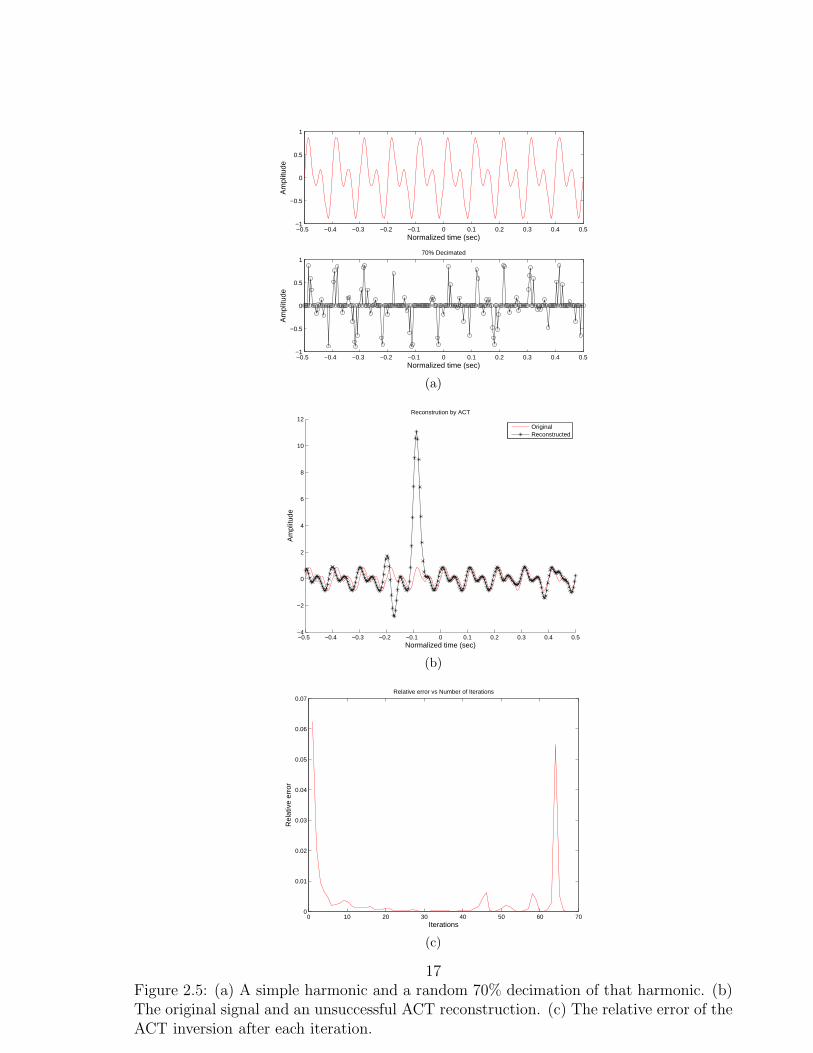
2.6 show three different random decimations of 70% of the traces. The ACT method

performs well on the first trial, but breaks down on the second and third trials, resulting

in significant spurious events. On observing the sampling density in Figures 2.5a and

2.6a, and the corresponding reconstructions in Figures 2.5b and 2.6b, the large anomalous

peaks in the output correspond to large gaps in signal coverage. Note also that the

residual error in Figure 2.5c and Figure 2.6c decays exponentially at first, but then

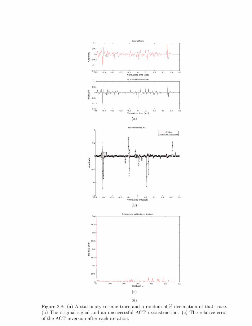
increases in peaks in the later iterations. Figure 2.7 shows a good reconstruction for the

seismic trace, randomly decimated by 30%, although the reconstruction departs from

the original signal in some places. At 50% decimation this method begins to fail on the

seismic trace, because the algorithm starts to map the noise to the higher frequencies

(Figure 2.8).

2.5 Conclusion

ACT method is a fast and accurate signal reconstruction method that is effective at

interpolating stationary signals with up to 50% of the samples missing. The method

begins to fail even on simple signals when decimation is increased to 70%, although the

reconstruction can be successful if the gaps in signal coverage are not too extreme.

14

−0.5 −0.4 −0.3 −0.2 −0.1 0 0.1 0.2 0.3 0.4 0.5−1

−0.5

0

0.5

1

Normalized time (sec)

Am

plitu

de

−0.5 −0.4 −0.3 −0.2 −0.1 0 0.1 0.2 0.3 0.4 0.5−1

−0.5

0

0.5

1

Normalized time (sec)

Am

plitu

de

40% Decimated

(a)

−0.5 −0.4 −0.3 −0.2 −0.1 0 0.1 0.2 0.3 0.4 0.5−1

−0.8

−0.6

−0.4

−0.2

0

0.2

0.4

0.6

0.8

1

Normalized time (sec)

Am

plitu

de

Reconstrution by ACT

OriginalReconstructed

(b)

0 2 4 6 8 10 12 14 16 180

0.01

0.02

0.03

0.04

0.05

0.06

0.07

Iterations

Rel

ativ

e er

ror

Relative error vs Number of Iterations

(c)

Figure 2.3: (a) A simple harmonic and a random 40% decimation of that harmonic. (b)The original signal the ACT reconstruction. (c) The relative error of the ACT inversionafter each iteration.

15

−0.5 −0.4 −0.3 −0.2 −0.1 0 0.1 0.2 0.3 0.4 0.5−1

−0.5

0

0.5

1

Normalized time (sec)

Am

plitu

de

−0.5 −0.4 −0.3 −0.2 −0.1 0 0.1 0.2 0.3 0.4 0.5−1

−0.5

0

0.5

1

Normalized time (sec)

Am

plitu

de

70% Decimated

(a)

−0.5 −0.4 −0.3 −0.2 −0.1 0 0.1 0.2 0.3 0.4 0.5−1

−0.8

−0.6

−0.4

−0.2

0

0.2

0.4

0.6

0.8

1

Normalized time (sec)

Am

plitu

de

Reconstrution by ACT

OriginalReconstructed

(b)

0 10 20 30 40 50 60 70 800

0.01

0.02

0.03

0.04

0.05

0.06

0.07

Iterations

Rel

ativ

e er

ror

Relative error vs Number of Iterations

(c)

Figure 2.4: (a) A simple harmonic and a random 70% decimation of that harmonic. (b)The original signal and a successful ACT reconstruction. (c) The relative error of theACT inversion after each iteration.

16

−0.5 −0.4 −0.3 −0.2 −0.1 0 0.1 0.2 0.3 0.4 0.5−1

−0.5

0

0.5

1

Normalized time (sec)

Am

plitu

de

−0.5 −0.4 −0.3 −0.2 −0.1 0 0.1 0.2 0.3 0.4 0.5−1

−0.5

0

0.5

1

Normalized time (sec)

Am

plitu

de

70% Decimated

(a)

−0.5 −0.4 −0.3 −0.2 −0.1 0 0.1 0.2 0.3 0.4 0.5−4

−2

0

2

4

6

8

10

12

Normalized time (sec)

Am

plitu

de

Reconstrution by ACT

OriginalReconstructed

(b)

0 10 20 30 40 50 60 700

0.01

0.02

0.03

0.04

0.05

0.06

0.07

Iterations

Rel

ativ

e er

ror

Relative error vs Number of Iterations

(c)

Figure 2.5: (a) A simple harmonic and a random 70% decimation of that harmonic. (b)The original signal and an unsuccessful ACT reconstruction. (c) The relative error of theACT inversion after each iteration.

17

−0.5 −0.4 −0.3 −0.2 −0.1 0 0.1 0.2 0.3 0.4 0.5−1

−0.5

0

0.5

1

Normalized time (sec)

Am

plitu

de

−0.5 −0.4 −0.3 −0.2 −0.1 0 0.1 0.2 0.3 0.4 0.5−1

−0.5

0

0.5

1

Normalized time (sec)

Am

plitu

de

70% Decimated

(a)

−0.5 −0.4 −0.3 −0.2 −0.1 0 0.1 0.2 0.3 0.4 0.5−10

0

10

20

30

40

50

60

70

Normalized time (sec)

Am

plitu

de

Reconstrution by ACT

OriginalReconstructed

(b)

0 20 40 60 80 100 1200

0.01

0.02

0.03

0.04

0.05

0.06

0.07

Iterations

Rel

ativ

e er

ror

Relative error vs Number of Iterations

(c)

Figure 2.6: (a) A simple harmonic and a random 70% decimation of that harmonic. (b)The original signal and an unsuccessful ACT reconstruction. (c) The relative error of theACT inversion after each iteration.

18

−0.5 −0.4 −0.3 −0.2 −0.1 0 0.1 0.2 0.3 0.4 0.5−0.15

−0.1

−0.05

0

0.05

0.1

Normalized time (sec)

Am

plitu

de

Original Trace

−0.5 −0.4 −0.3 −0.2 −0.1 0 0.1 0.2 0.3 0.4 0.5−0.1

−0.05

0

0.05

0.1

Normalized time (sec)

Am

plitu

de

30 % Random decimation

(a)

−0.5 −0.4 −0.3 −0.2 −0.1 0 0.1 0.2 0.3 0.4 0.5−0.15

−0.1

−0.05

0

0.05

0.1

Normalized time(sec)

Am

plitu

de

Reconstrution by ACT

OriginalReconstructed

(b)

0 10 20 30 40 50 60 70 80 900

0.005

0.01

0.015

0.02

0.025

0.03

0.035

0.04

Iterations →

Rel

ativ

e er

ror

Relative error vs Number of Iterations

(c)

Figure 2.7: (a) A stationary seismic trace and a random 30% decimation of that trace.(b) The original signal and a successful ACT reconstruction. (c) The relative error of theACT inversion after each iteration.

19

−0.5 −0.4 −0.3 −0.2 −0.1 0 0.1 0.2 0.3 0.4 0.5−0.15

−0.1

−0.05

0

0.05

0.1

Normalized time (sec)

Am

plitu

de

Original Trace

−0.5 −0.4 −0.3 −0.2 −0.1 0 0.1 0.2 0.3 0.4 0.5−0.15

−0.1

−0.05

0

0.05

0.1

Normalized time (sec)

Am

plitu

de

50 % Random decimation

(a)

−0.5 −0.4 −0.3 −0.2 −0.1 0 0.1 0.2 0.3 0.4 0.5−1.5

−1

−0.5

0

0.5

1

Normalized time(sec)

Am

plitu

de

Reconstrution by ACT

OriginalReconstructed

(b)

0 100 200 300 400 500 6000

0.005

0.01

0.015

0.02

0.025

0.03

0.035

0.04

Iterations →

Rel

ativ

e er

ror

Relative error vs Number of Iterations

(c)

Figure 2.8: (a) A stationary seismic trace and a random 50% decimation of that trace.(b) The original signal and an unsuccessful ACT reconstruction. (c) The relative errorof the ACT inversion after each iteration.

20

Chapter 3

Kaiser Bessel gridding kernel for seismic data

regularization

3.1 Summary

There are numerous approach which deal with the interpolation of missing samples in

seismic data. The proposed Kaiser Bessel non uniform Fast Fourier transform (NFFT)

kernel is new in its kind as it balances between the accuracy and computational cost.

Use of Kaiser Bessel (NFFT) kernel is new for seismic data regularization.

The application of Bessel kernel for non uniform samples is not a new algorithm, but

it is an approximation scheme that can be used to calculate an approximate spectrum.

In one dimension, computational complexity of Kaiser Bessel NFFT is O(NlogN) which

is a dramatic improvement from the O(N2) complexity of the Discrete Fourier transform

(DFT), and comparable to Fast Fourier transform (FFT). This algorithm can be easily

extended to higher dimensions. Least squares is used to refine an approximated spec-

tra followed by simple Inverse Fast Fourier transform (IFFT). The applicability of the

proposed method is examined using synthetic examples.

3.2 Introduction

In this chapter for the seismic data reconstruction, the Kaiser Bessel window function

is used. Combining the window function with Fast Fourier transform will give us the

Kaiser Bessel non uniform Fourier kernel. The need of a non uniform kernel is based

on the constrain that Fast Fourier transform (FFTs) needs regular spacing for its ap-

21

plication. Non uniform Fast Fourier transforms (NFFT) which are generalizations for

the FFT are discussed by many authors in the past (Dutt and Rokhlin, 1993; Steidl,

1998; Duijndam and Schonewille, 1999; Lee and Greengard, 2006). It is important to

stress that the Non uniform Fourier kernel is been used for seismic data reconstruction

by Duijndam and Schonewille (1999) using B - spline and Gaussian window functions,

but Kaiser Bessel window has never been tested. Proposed Kaiser Bessel based Kernel

balances between the computational resources and reported to give better result than

Gaussian and B- Spline window based kernels, and already been tested in Medical imag-

ing (Knopp et al., 2007).

3.3 Theory

In the case of non uniform sampling, direct discretization of the forward transformation

corresponding to the irregular grid at hand will be highly erroneous. A better approach

will be taking the exact inverse transform from the regularly sampled domain to irregu-

larly sampled domain and use this as a forward model in an inverse problem. The general

form can be written in term of matrix vector notation as

Am = d (3.1)

Where, Amxn is the forward model, d is the observation vector in time domain consist

of true values and m represents Fourier components. Observation vector is irregular

sampled spatial value in case of seismic data reconstruction and finally x is a unknown

solution. In bandlimited approach, it will always be a over determined problem. General

least square solution for such approach will be

m = (A∗A)−1A∗d, (3.2)

22

Where, A is mapping matrix from one domain to another domain and A* represents

its complex conjugate transpose.

This is basic approach for hyperbolic Radon transform and linear Radon transform

by Thorson and Claerbout (1985). If desired, data estimated in the Fourier domain can

be transform back to a regular grid in the spatial domain using inverse fast Fourier

transform.

3.3.1 Discrete Fourier Transform

The general form of the forward discrete Fourier transform in case of the regular sampling

can be defined as

Pm =

N−1∑

j=0

Pje−2πinm/N (m = 0, · · · , N − 1), (3.3)

Where, Pm are the Fourier coordinates and Pj denotes the input signal.

Assuming the regular sampling the transform can be easily inverted as,

Pj =

N−1∑

n=0

Pme2πinm/N . (3.4)

Here, e2πinm/N is known as the data mapping kernel. All entries of this data mapping

kernel are orthogonal to each other in case of regular sampling.

The forward Discrete Fourier transform (DFT) for regularly sampled seismic data

(Duijndam et al., 1999) can be written to include sample spacing as

P (kx, ω) = ∆x

N−1∑

n=0

P (n∆x, ω) e−ink∆x, (3.5)

where ω is the temporal frequency, ∆x is sample interval in spatial domain and kx is

the wave number. Regular sampling in spatial domain enforces periodicity.

In Equation 3.5, to avoid aliasing after the Fourier transform, it is required to keep

∆x small. For avoiding aliasing and maintaining economics of seismic survey, it is always

23

better to restrict the sampling based on Shannon sampling theory (Unser, 2000). DFT is

the mapping of N point signal (x1, x2, · · ·xN ) in to N Fourier coefficients XK . In matrix

vector form the DFT can be denoted as

X = DFT ∗ x, (3.6)

DFT is a Fourier matrix that maps N dimensional vector x in to another N dimensional

vector X. To transform back to the spatial domain, need DFT−1, which is inverse DFT

Matrix. The inverse discrete Fourier Transform is defined by

P (x, ω) =∆k

2π

m=M∑

m=−M

P (m∆k, ω) e−im∆kx, (3.7)

where ∆k is the sampling interval in Fourier domain, where N = 2M+1 and ∆k = 2πN∆x

.

The matrix vector form of equation 3.7 is

x = DFTH ∗X, (3.8)

where DFTH is the Hermitian adjoint of DFT, Since sampling is regular, DFTN×N is

orthogonal, which implies

DFTH ∗DFT = NIN , (3.9)

where IN is N dimensional identity matrix. Equation 3.9 shows that DFT is an orthog-

onal transformation, and that the inverse is computed using a Hermitian operator. The

cost of inverting N ×N Hermitian operator is O(N2) instead of O(N3). Cost is further

diminished to O(NlogN)using the fast Fourier transform (FFT) instead of matrix vector

multiplication. However, FFT can’t be applied in the case of irregular sampling

DFTH ∗DFT 6= NIN , (3.10)

24

Equation 3.10 shows that when sampling is irregular, it is not simple to invert the

DFT matrix, since columns of the DFT matrix is no longer orthogonal. The approxima-

tion converging closest to DFT for irregular sampling is the weighted Fourier Transform

(DFT).

P (m∆k, ω) =N−1∑

n=0

P (xn, ω)ejm∆kxn∆xn, (3.11)

where ∆k is the regular sample interval in Fourier domain. xn represents the positions

of the irregular nodes, and ∆xn is the weighting factor which depends upon the distance

between the samples in spatial domain.

∆xn =xn+1 − xn−1

2, n = 0, ......., N − 1. (3.12)

The DFT in Equation 3.11 , however, is not a unitary transformation, as it fails the

dot product test (i:e the dot product of two vectors before the transformation should

be equal to dot product after the transformation). For this reason, it is not possible to

reconstruct the original domain by a simple inverse FFT (IFFT).

Feichtinger et al. (1995b) suggests an approach to handle the irregular grid problem

by putting a band limitation restrain on the data. If ∆k is the sampling interval in

Fourier domain than the data is band limited to between [−M∆k,M∆k]. Accordingly,

equation 3.4 for N irregular samples (x0, x1 · · · , xN−1) can be denoted in matrix vector

notation as

y = Ap, (3.13)

where,

yn = P (xn, ω). (3.14)

Where, yn represents the values on the non uniform grid. Also,

pm = P (m∆k, ω), (3.15)

25

Anm =∆k

2πe−jm∆kxn. (3.16)

Where, pm is the solution for the linear least square problem and Anm is the data mapping

kernel. However, real data is never band limited; there will always be some spatial

frequencies above the restricted bandwidth. It can be treated as noise in the forward

model and can be included in equation 4.1 as

y = Ap+Noise, (3.17)

Further, p can be estimated by

p =(

AHWA+ k2I)−1

AHWy, (3.18)

where W is a weight matrix, k is the stabilization factor and AH is the complex conjugate

transpose of A. From equation’s 4.2, 4.3, and 4.4, the last term of equation 3.18 can be

written as

AHWy =∆k

2π

N−1∑

n=0

P (xn, ω)ejm∆kxnWnn, (3.19)

where Wnn = ∆xn. Here, except for constant∆k2π, equation 3.19 is equivalent to equation

3.11, which represents weighted DFT. Estimated Fourier spectrum p can be transformed

back to the spatial domain by direct inverse transform. The DFT is a major compu-

tational task for the forward transform, as computational complexity of the DFT is

O(N2). Many inversion schemes that are use in data processing (Sacchi et al., 1998;

Sacchi and Ulrych, 1996) rely on the solution of normal equations on the right hand side

of which is DFT.

Proposed kaiser Bessel kernel is a solution that can replace slow DFT with faster

algorithm. Fast algorithm will make many algorithms where DFT is used as practical

for industry.

26

3.4 Methodology

Methodology is divided into two categories forward problem and inverse problem. Both

is calculated using NFFT Kaiser Bessel kernel. Methodology can be divided in following

steps

1. AHWy = b, calculates direct forward transform using NFFT kernel.

2. U = (AHWA + k2I), computation of deconvolution operator, using NFFT and

Adjoint NFFT kernels.

3. Up = b, calculates least squares system for p.

4. y1 = IFFT (p) calculates direct backward transform on regular grid using Fast

IFFT.

3.4.1 Forward problem

The Non uniform Fast Fourier gridding algorithm can be numerically expressed in fol-

lowing steps: gridding, FFT, deconvolution. The gridding is obtained by convolution

of the sampled signal values with a convolution function followed by re-sampling onto a

cartesian grid. Convolution with Kaiser Bessel kb(x) is carried out to make the signal

approximately band-limited according to

pg(m) = kb(x) ∗ p(x), (3.20)

where pg(m) is the result of spatial convolution. Equation 3.20 can be written as multi-

plication in the Fourier domain as

Pg(m) = KB(m)× P (m), (3.21)

27

where Pg(m) is the Fourier spectrum of pg(m) in Fourier domain. For efficiency,

Kaiser Bessel need to be truncated, thus generating n samples for pg(m) where

n = −int

(

q + 1

2

)

+ 1, · · · , N + int

(

q + 1

2

)

− 1, (3.22)

and where int(x) truncates to the largest integer smaller than x for x ≥ 0. The algorithm

is initialized at pg(n) = 0, where subscript g indicates an application of Kaiser Bessel

filter and keep updating by summation of the N shifted filters. This summation of N

shifted filter can be given by

pg(n)← pg(n) + ∆xpnkb(n∆x− xn) (3.23)

Equation 3.23 represents mapping of the irregular samples on to a regular grid. The

sampling pg(n) = ∆xp1(n∆x) is similar to equation 3.24 in Fourier domain which can be

written as

Pg(m) =∑

I∈Z

P (m+ IN)KB(m+ IN) (3.24)

When Pg(m) is broadband, aliasing will occur when KB(m + IN) 6= 0 for any I 6= 0.

It is suggested (Duijndam and Schonewille, 1999) that to remove the aliasing, there is

requirement of making the signal periodic.

pg(n) =∞∑

I=−∞

pg(n+ IN), n = 0, 1, 2, · · · , N − 1, (3.25)

where pg(n + lN) = 0 is outside the interval given by equation 3.22. Convolution of the

signal followed by the discrete transform can be represented by

Pg(m)FFT =

N−1∑

n=0

pg(n)ej2πnm/N , m =

N

2, · · · ,

N

2− 1 (3.26)

where Pg(m)FFT is the spectrum obtained using the FFT. Finally correction for convo-

lution is carried out by deconvolution in Fourier domain according to

P (m) =Pg(m)FFT

KB(m), (3.27)

where P (m) is the approximate spectrum and KB(m) is Fourier domain representation

of Bessel filter.

28

3.4.2 Window function

NFFT algorithms are based on convolution of sampled signal with a band limiting fil-

ter, and several different names are indicated in the literature. Jackson et al. (1991)

discuss these algorithms in terms of image processing and refer to them as griding al-

gorithms. Beylkin et al. (1991) proposes a similar irregular Fourier transform algorithm

where convolution with B-spline is carried out to make the signal approximately band

limited. Jackson et al. (1991) discussed several forms of filters which can be used, and a

truncated Gauss filter is introduced by Dutt and Rokhlin (1993).

Most of the recent development in these algorithms deals with optimization of above

windows functions, but still the Kaiser Bessel window function gives the best result

(Knopp et al., 2007).

Kaiser Bessel window function

Prolate Spheroidal wave function (PSWF) has finite time support and maximum con-

centration of energy within a given bandwidth. The PSWF is the eigenfunction having

the largest eigenvalue of the operation of repeatedly low-pass filtering a function and

band-limiting it. It is difficult to compute but the Kaiser Bessel function is a close ap-

proximation of the PSWF. For a given filter q∆x and bandwidth B, the least amount of

energy outside desired passband i:e minimization of

∫

|m|>B|g(m)|2dm

∫∞

∞|g(m)|2dm

. (3.28)

Kaiser Bessel function can be represented as (Knopp et al., 2007)

g(x) =1

q∆xIoβ

√

1−

(

2x

q∆x

)2−q∆x

2≤ x ≤

q∆x

2, (3.29)

Where Io is the zeroth order modified Bessel function of its first kind. In Frequency

domain, its Fourier transform is used for deconvolution purpose. Fourier domain repre-

29

sentation of Kaiser Bessel function can be written as

g(m) =sin(

√

π2(q(∆x)2m2 − β2)√

π2(q(∆x)2m2 − β2. (3.30)

Figure 3.1a represents Kaiser Bessel window for various value of β in spatial domain.

β is the parameter for Kaiser window, which gives control over trade off between main

lobes width and side lobes level. Large β gives wider main lobe but lower side lobes as

shown in Figures 3.1a and 3.1b. For maximum frequency resolution, always narrowest

main lobe is preferred. Jackson et al. (1991) carried out detailed analysis of the various

convolution functions leading to the approximation for the prolate spheroidal function.

Different value of β is suggested for 3.30 in (Jackson et al., 1991). For all calculation

purpose value of q is taken as 6 and value of β = 2. These values are taken as a optimum

by (Knopp et al., 2007).

10 20 30 40 50 600

0.1

0.2

0.3

0.4

0.5

0.6

0.7

0.8

0.9

1

Filter length →

Nor

mal

ized

Am

plitu

de

beta=1beta = 3beta=5beta=7

(a)

0 0.1 0.2 0.3 0.4 0.5 0.6 0.7 0.8 0.9 1−250

−200

−150

−100

−50

0

50

Normalized Frequency (×π rad/sample)

Mag

nitu

de (

dB)

beta=1beta = 3beta=5beta=7

(b)

Figure 3.1: Kaiser Bessel filter. a) Kaiser window in spatial domain. b) Kaiser windowin Fourier domain.

30

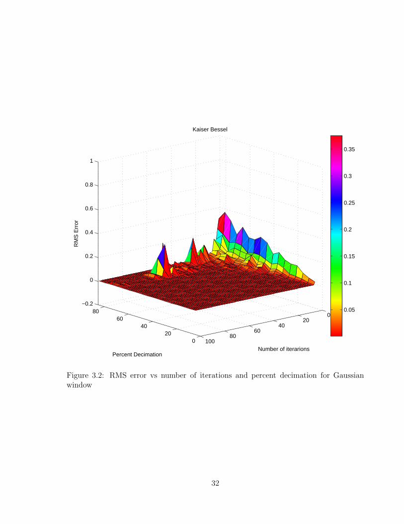
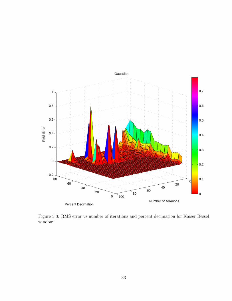
3.4.3 Comparision

To assess accuracy and computational complexity in signal reconstruction, comparisons

are made with the traditional gaussian method in the framework of NFFT. Figures 3.2

and 3.3 show a comparative study of the above two algorithms. I tested the performance

of each algorithm with a very limited dataset which require maximum 100 iteration for

converging to solution. The test is performed on signal composed of random number

of harmonics with 512 samples with sampling rate of .01ms. Decimation is performed

with a 5% increment which decimate the signal beginning from 5% to 85%. At low

decimation rate both Gaussian and Kaiser Bessel converge to the solution at faster rate

with minimum number of iterations. The RMS error during the initial stages of iteration

between 5% to 25% decimation did not show much difference for the two algorithms. After

25% of decimation, the Gaussian starts giving high error values for first few iteration when

compared with Kaiser Bessel. Figure 3.2 shows that solution is converging to a unstable

solution with higher error values where as Kaiser Bessel is giving us a stable solution with

low error values. At the higher decimation rate Kaiser Bessel algorithm outperforms the

Gaussian by converging smoothly at 50 % to 75 % decimation with low error values for

number of iterations lies between 20 and 40. On the other hand, Gaussian starts failing

giving higher error peaks while converging with higher number of iterations between 60

and 80 as illustrated on the left side of figure 3.3.

In summary, Gaussian is not suitable for higher decimation rate when compared to

Kaiser Bessel. On the other hand, Kaiser Bessel performs better, in terms of accuracy

and stability at higher decimation. This comparison leads to a decision of using Kaiser

Bessel filter as the main kernel for implementation of NFFT for regularization problem.

31

020

4060

800

2040

6080

100

−0.2

0

0.2

0.4

0.6

0.8

1

Number of iterarions

Kaiser Bessel

Percent Decimation

RM

S E

rror

0.05

0.1

0.15

0.2

0.25

0.3

0.35

Figure 3.2: RMS error vs number of iterations and percent decimation for Gaussianwindow

32

020

4060

800

2040

6080

100

−0.2

0

0.2

0.4

0.6

0.8

1

Number of iterarions

Gaussian

Percent Decimation

RM

S E

rror

0

0.1

0.2

0.3

0.4

0.5

0.6

0.7

Figure 3.3: RMS error vs number of iterations and percent decimation for Kaiser Besselwindow

33

3.4.4 Inversion

In general underdetermined linear system will solve in this problem, so the solution can

only be approximated up to a residual of the form

r = y − Ap. (3.31)

In order to compensate for the missing samples it is important to incorporate a weight

function W, W > 0 and the problem becomes a

argmin||y − Ap||2W =

M−1∑

j=0

wj|yj − f(xj)|2 → min, (3.32)

where W =diag(wj)j=0,··· ,M−1

3.5 Efficiency

The problem of regularization in the least squares NFFT framework is divided in two cat-

egories: forward method and inversions. The direct forward transform is been computed

using NFFT which is AH and for the inversion purpose operator U = (AHWA+ k2I) is

computed. For computing the inversion operator, the forward Fourier kernel AH and its

adjoint A is already computed using NFFT. It has already been that NFFT give a com-

putational advantage over DFT. Further more iterative solution of 3.32 has been analysis

in detail in large number of papers (Feichtinger et al., 1995b). The adaptive weights con-

jugate gradient Toeplitz method (ACT) applies the conjugate gradient method to the

weighted normal equation which can be written as

AHWAp = AHWy. (3.33)

34

3.6 Synthetic Tests

3.6.1 Synthetic 1D examples

Purpose of any reconstruction algorithm can only be solved if it is tested as general

algorithm. Its important stress that not all the methods are capable of dealing with

regular as well as irregular sampling. In fact, most of the parametric signal reconstruction

technique fails to deal with irregular sampling (Naghizadeh and Sacchi, 2008b,c, 2009b;

Hennenfent and Herrmann, 2008, 2007).

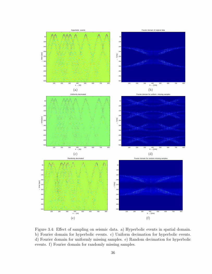
Figure 3.4 demonstrates effect of the sampling on seismic data. Synthetic hyperbolic

events (Figure 3.4a) and its Fourier domain representation (Figure 3.4b). In case of

regular decimation (Figure 3.4d), strong coherent noise (Figure 3.4d) will be created due

to acquisition. Noise is highly structured with strong amplitudes. Most of the regular

interpolation techniques is based on the idea of using non aliased low frequency and

de-alias higher frequency. (Abma and Kabir, 2005) pointed out that most interpolation

method based on regular sampling whereas irregular sampling generate weak noise. In

irregular sampling (Figure 3.4e), power is focused at few Fourier coefficients and noise is

spread whole transform domain (Figure 3.4f). Sparser the signal, straightforward will be

the reconstruction.

For examining the performance of Kaiser Bessel NFFT algorithm with various sam-

pling operators, created a simple sin signal in Figure 3.5 as well as another signal in

Figure 3.6 which is composed of two harmonics. Detailed analysis with varying gaps,

extrapolation, random sampling and uniform sampling is carried out.

For 1 dimension examples will take case of simple sinusoidal with 256 samples, at

sampling rate of 10ms. Top panel will show the decimated spatial domain and panel below

it is reconstructed missing samples. Figure 4.1a shows the 30 % randomly decimated

signal and reconstructed sinusoidal. Even with 50% randomly decimation in Figure

35

x → (m)

← ti

me

(sec

)

Hyperbolic events

100 200 300 400 500 600 700 800

50

100

150

200

250

300

350

400

450

500

(a)

Fourier domain of original data

k → (1/m)

← f

(H

z)

100 200 300 400 500 600 700 800

50

100

150

200

250

300

350

400

450

500

(b)Uniformly decimated

x → (m)

← ti

me(

sec)

100 200 300 400 500 600 700 800

50

100

150

200

250

300

350

400

450

500

(c)

Fourier domain for uniform missing samples

k → (1/m)

← f

(Hz)

100 200 300 400 500 600 700 800

50

100

150

200

250

300

350

400

450

500

(d)Randomly decimated

x → (m)

← ti

me

(sec

)

100 200 300 400 500 600 700 800

50

100

150

200

250

300

350

400

450

500

(e)

Fourier domain for random missing samples

k → (1/m)

← f

(Hz)

100 200 300 400 500 600 700 800

50

100

150

200

250

300

350

400

450

500

(f)

Figure 3.4: Effect of sampling on seismic data. a) Hyperbolic events in spatial domain.b) Fourier domain for hyperbolic events. c) Uniform decimation for hyperbolic events.d) Fourier domain for uniformly missing samples. e) Random decimation for hyperbolicevents. f) Fourier domain for randomly missing samples.

36

0 0.5 1 1.5 2 2.5 3−1

−0.5

0

0.5

1

x (m)→

Am

plitu

de

Decimated Harmonic

Decimated

0 0.5 1 1.5 2 2.5 3−1

−0.5

0

0.5

1

x (m)→

Am

plitu

de

Reconstructed Harmonic

(a)

0 0.5 1 1.5 2 2.5 3−1

−0.5

0

0.5

1

x (m)→

Am

plitu

de

Decimated Harmonic

Decimated

0 0.5 1 1.5 2 2.5 3−1

−0.5

0

0.5

1

x (m)→

Am

plitu

de

Reconstructed Harmonic

(b)

0 0.5 1 1.5 2 2.5 3−1

−0.5

0

0.5

1

x (m)→

Am

plitu

de

Decimated Harmonic

Decimated

0 0.5 1 1.5 2 2.5 3−1

−0.5

0

0.5

1

x (m)→

Am

plitu

de

Reconstructed Harmonic

(c)

0 0.5 1 1.5 2 2.5 3−1

−0.5

0

0.5

1

x (m)→

Am

plitu

de

Decimated Harmonic

Decimated

0 0.5 1 1.5 2 2.5 3−1

−0.5

0

0.5

1

x (m)→

Am

plitu

de

Reconstructed Harmonic

(d)

Figure 3.5: Reconstruction for Harmonics. a) Harmonics with 30 % decimation. b)Harmonics with 50 % decimation. c) Harmonics with 60 % decimation. d) Harmonicswith 80 % decimation.

4.1b algorithm seems to do pretty well. On implementing high decimation sampling

functions of 60% in Figure 3.5c results are good, all missing samples have been successfully

reconstructed. On going further decimation in Figure 3.5d due to lost of the Fourier

coefficients it is not able to reconstruct the same amplitude back, except at one point

where it is missing most of the samples.

37

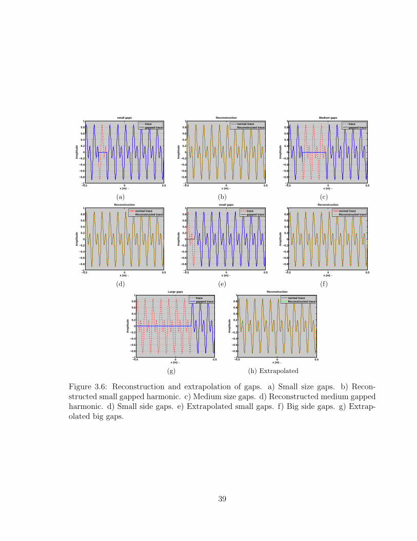
3.6.2 Gaps

In the previous test, it has been observed that algorithm fails some time when more

number of Fourier coefficients are missing from a single location. This behaviour is

further tested in gap test. In this different gaps will be created by taking more number

of Fourier coefficients from a single location. Algorithm is tested for all size of gaps. Input

signal composed of two harmonics , with sampling interval of 10ms for 256 samples. In

case of small gaps in Figure 3.6b, reconstruction is perfect. Even in the presence of large

gaps in Figure 3.6d, algorithm works effectively.

38

−0.5 0 0.5−1

−0.8

−0.6

−0.4

−0.2

0

0.2

0.4

0.6

0.8

1

x (m)→

Am

plitu

de

small gaps

tracegapped trace

(a)

−0.5 0 0.5−1

−0.8

−0.6

−0.4

−0.2

0

0.2

0.4

0.6

0.8

1

x (m)→

Am

plitu

de

Reconstruction

normal traceReconstructed trace

(b)

−0.5 0 0.5−1

−0.8

−0.6

−0.4

−0.2

0

0.2

0.4

0.6

0.8

1

x (m)→

Am

plitu

de

Medium gaps

tracegapped trace

(c)

−0.5 0 0.5−1

−0.8

−0.6

−0.4

−0.2

0

0.2

0.4

0.6

0.8

1

x (m)→

Am

plitu

de

Reconstruction

normal traceReconstructed trace

(d)

−0.5 0 0.5−1

−0.8

−0.6

−0.4

−0.2

0

0.2

0.4

0.6

0.8

1

x (m)→

Am

plitu

de

small gaps

tracegapped trace

(e)

−0.5 0 0.5−1

−0.8

−0.6

−0.4

−0.2

0

0.2

0.4

0.6

0.8

1

x (m)→

Am

plitu

de

Reconstruction

normal traceReconstructed trace

(f)

−0.5 0 0.5−1

−0.8

−0.6

−0.4

−0.2

0

0.2

0.4

0.6

0.8

1

x (m)→

Am

plitu

de

Large gaps

tracegapped trace

(g)

−0.5 0 0.5−1

−0.8

−0.6

−0.4

−0.2

0

0.2

0.4

0.6

0.8

1

x (m)→

Am

plitu

de

Reconstruction

normal traceReconstructed trace

(h) Extrapolated

Figure 3.6: Reconstruction and extrapolation of gaps. a) Small size gaps. b) Recon-structed small gapped harmonic. c) Medium size gaps. d) Reconstructed medium gappedharmonic. d) Small side gaps. e) Extrapolated small gaps. f) Big side gaps. g) Extrap-olated big gaps.

39

3.6.3 Extrapolation

Extrapolation test is done for the reconstruction algorithm, purpose of algorithm is to

extrapolate the missing samples. Extrapolation is been tested on combination of two

harmonics for two categories, small gaps and large gaps in Figures 3.6e and 3.6g. Recon-

structed extrapolated harmonics can be seen in Figures 3.6f and 3.6h. Algorithms can

easily handle the stationary harmonics with large gaps. Algorithm can also be applied

on simple non stationary harmonics when taken small windows, and events are assumed

to be stationary.

3.7 Synthetic 2D examples

In case of 2D data reconstruction, the Fourier reconstruction is iterative on each fre-

quency slice in FK domain. NFFT least square will be applied on each frequency slice,

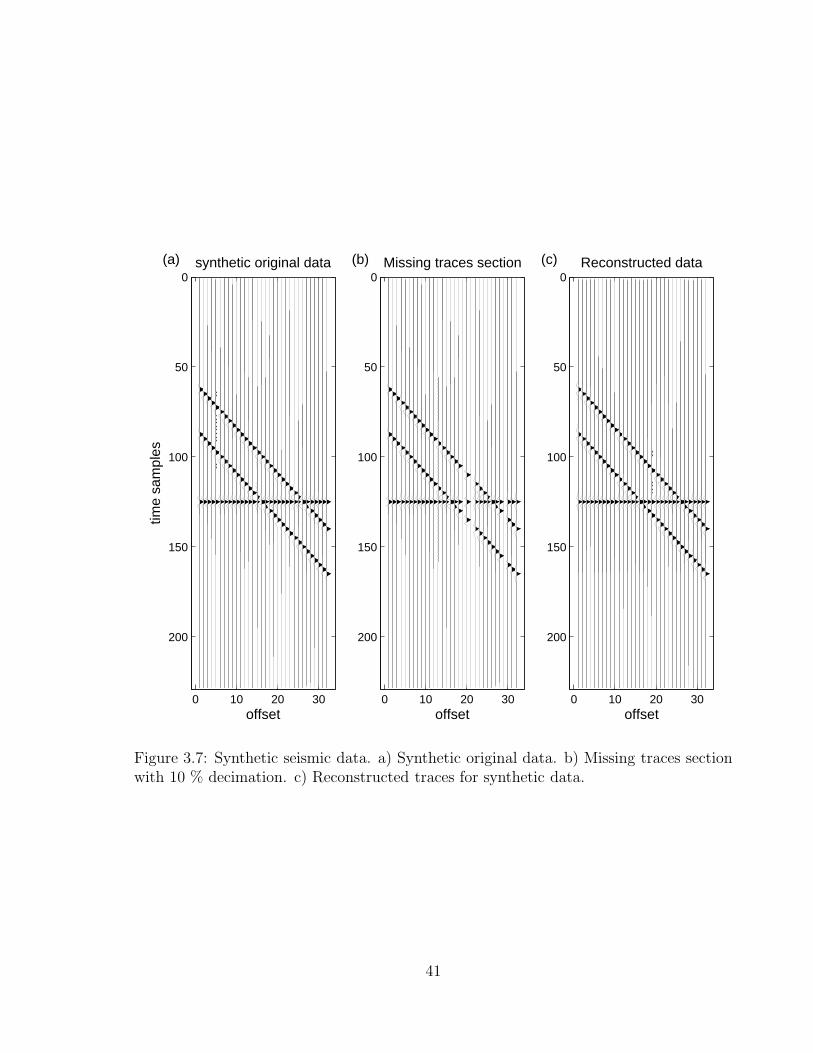
with iteratively moving to next slice. In Figure 3.7, there are three seismic events with

different dips and amplitudes. The seismic wavelet is ricker wavelet with peak frequency

of 50 Hz. Sampling rate for seismic data acquisition is 4ms. Figure 3.7 is an original

synthetic section. Figure 3.8 represents Fourier domain representation of original section.

Before testing algorithm for heavy decimation operators, its been tested for 10% random

decimation in Figure 3.8. NFFT least squares works perfectly in Figures 3.7 and 3.8 for

the small random decimation.

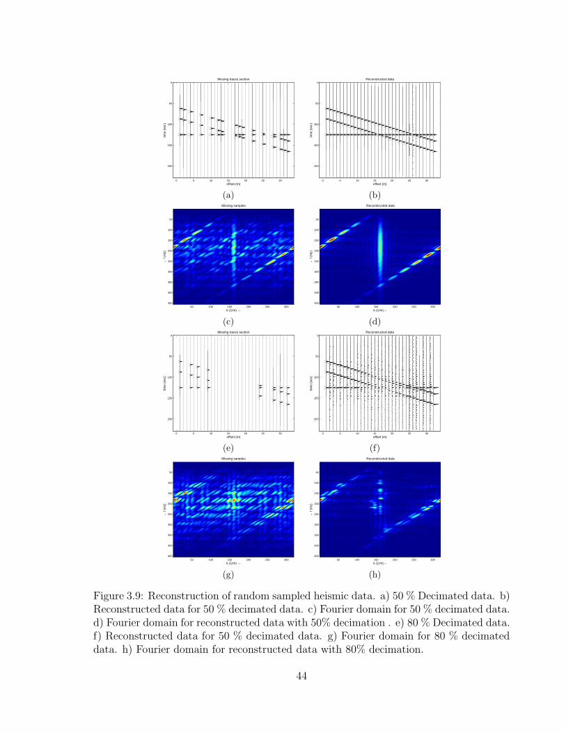
3.7.1 Randomly decimated dipping Events

Random sampling in the spatial domain (Figure 3.9a) can result in low amplitudes artifact

like in Figure (3.9c) along with the original Fourier events. The artifacts are the resultant

of random sampling operator which is 50% resultant due to decimation in original data

in Figure 3.9a. Reconstructed data in Figure 3.9b in case of 50% random decimation is

40

0 10 20 30

0

50

100

150

200

synthetic original data

offset

time

sam

ples

(a)

0 10 20 30

0

50

100

150

200

Missing traces section

offset

(b)

0 10 20 30

0

50

100

150

200

Reconstructed data

offset

(c)

Figure 3.7: Synthetic seismic data. a) Synthetic original data. b) Missing traces sectionwith 10 % decimation. c) Reconstructed traces for synthetic data.

41

Original data

← f

k→

(a)

100 200 300

50

100

150

200

250

300

350

400

450

Missing samples

← f

k→

(b)

100 200 300

50

100

150

200

250

300

350

400

450

Reconstructed data

← f

k→

(c)

100 200 300

50

100

150

200

250

300

350

400

450

Figure 3.8: Fourier domain representation. a) Fourier domain for original data. b) Fourierdomain for missing traces with 10 % decimation. c) Fourier domain for reconstructeddata. of original event with 10 % decimated data and reconstructed data.

42

as good as original. Figure 3.9b proves that algorithm works for the seismic section with

half of the missing samples. Even Fourier domain in Figure 3.9c shows all the energy

concentrated on the dipping events, with no energy getting dissipated.

Further moving to higher decimation of 80% in 3.9e low amplitudes artifacts are more

dominant. Along with the dominant artifacts, aliasing for the dips can be seen in Figure

3.9g. Noisy artifacts are observed in Figure 3.9f as compared to Figure 3.9b, it is because

of the big gap in Figure 3.9e. It was seen before that algorithm works for big gaps in

case of simple harmonics in Figures (3.6b, 3.6d), but it is effective even in case of linear

dipping events. It is important to test when algorithm fails for knowing its limitation.

Therefore final data is tested using random sampling operators of 80% decimations in

Figure3.9f. Figure 3.9e shows 80% decimated data, with its Fourier domain in Figure

3.9g. It should be noticed that Fourier domain of 80% decimation in Figure 3.9g has

more aliased events than with 50% decimation, it is again due to the presence of more

gaps in the decimated section in Figure 3.9e as comparison to 50% decimation in Figure

3.9a. Algorithm started to fails with 80% decimation as seen in reconstructed section in

Figures 3.9f, there are low amplitudes artifacts in the recovered Fourier domain (Figure

3.9h) as well. Events in recovered section are still well defined (Figure 3.9f) but with the

high amplitude noise in the section. Both reconstructed, t-x domain and f-k domain in

Figure 3.9f and Figure 3.9h demonstrates the limitation of the algorithm.

3.7.2 Uniform decimation for dipping events

In order to generalize the algorithm for the interpolation, testing will be carried out with

the uniformly decimation operators. Parametric reconstruction technique seems not to

perform very well, when implemented on the uniformly decimated seismic section. In

case of uniform decimation, replicas of events are created in the Fourier domain which

is difficult to separate. But with the band-limiting approach like least square NFFT,

43

0 5 10 15 20 25 30

0

50

100

150

200

Missing traces section

time

(sec

)

offset (m)

(a)

0 5 10 15 20 25 30

0

50

100

150

200

Reconstructed data

offset (m)

time

(sec

)

(b)Missing samples

← f

(Hz)

k (1/m) →50 100 150 200 250 300

50

100

150

200

250

300

350

400

450

(c)

Reconstructed data

← f

(Hz)

k (1/m)→50 100 150 200 250 300

50

100

150

200

250

300

350

400

450

(d)

0 5 10 15 20 25 30

0

50

100

150

200

Missing traces section

time

(sec

)

offset (m)

(e)

0 5 10 15 20 25 30

0

50

100

150

200

Reconstructed data

offset (m)

time

(sec

)

(f)Missing samples

← f

(Hz)

k (1/m) →50 100 150 200 250 300

50

100

150

200

250

300

350

400

450

(g)

Reconstructed data

← f

(Hz)

k (1/m)→50 100 150 200 250 300

50

100

150

200

250

300

350

400

450

(h)

Figure 3.9: Reconstruction of random sampled heismic data. a) 50 % Decimated data. b)Reconstructed data for 50 % decimated data. c) Fourier domain for 50 % decimated data.d) Fourier domain for reconstructed data with 50% decimation . e) 80 % Decimated data.f) Reconstructed data for 50 % decimated data. g) Fourier domain for 80 % decimateddata. h) Fourier domain for reconstructed data with 80% decimation.

44

replicated spectrum of event can be isolated in the low frequency of data. Its because of

the higher power spectrum at low frequencies. Uniform decimation factors of 2 in Figure

3.10a and of 4 in Figure 3.10e are implemented.

2D Synthetic section is decimated by a factor 2 in Figure 3.10a. Exact replicas of

planar and dipping events are created in FK domain of Figure 3.10c. Reconstructed data

in Figure 3.10b and its Fourier domain in Figure 3.10d is recovered. On increasing the

decimation factor to 4 in Figure 3.10e, have more replicas of planar and dipping events

in Figure 3.10h as compare to 3.10d. But the recovered data in Figure 3.10f has well

define events like in Figure 3.10f, setting reputation of algorithm to work on uniformly

decimated data as well. Further for uniform sampling, like random sampling there is

need of minimum number of samples so that algorithm can recover the data.

3.7.3 Hyperbolic events

In case of hyperbolic events in Figure 3.11, data can always be windowed thus assuming

that events are linear. But, already seen the application of least square NFFT on linear

events. Applying LS-NFFT on the decimated data without windowing in Figure 3.11a.

In upper part of reconstructed data in Figure 3.11b apexes are successfully reconstructed.

But still some high amplitude noise is observed.

3.8 Conclusion

Low computational cost of least square NFFT make it a robust and practical algorithm.

This method successfully reconstruct the missing samples. This algorithm is effective

both in case of random sampled data as well as uniform sampling. Algorithm can be

easily extended to higher dimensions, and it will prove to be cost effective even for it.

Though it is able to reconstruct the curved events. But a good windowing strategy which

enforces linearity for curved events will sure provide better results in that case. NFFT

45

0 5 10 15 20 25 30

0

50

100

150

200

Missing traces section

time

(sec

)

offset (m)

(a)

0 5 10 15 20 25 30

0

50

100

150

200

Reconstructed data

offset (m)

time

(sec

)

(b)Missing samples

← f

(Hz)

k (1/m) →50 100 150 200 250 300

50

100

150

200

250

300

350

400

450

(c)

Reconstructed data

← f

(Hz)

k (1/m)→50 100 150 200 250 300

50

100

150

200

250

300

350

400

450

(d)

0 5 10 15 20 25 30

0

50

100

150

200

Missing traces section

time

(sec

)

offset (m)

(e)

0 5 10 15 20 25 30

0

50

100

150

200

Reconstructed data

offset (m)

time

(sec

)

(f)Missing samples

← f

(Hz)

k (1/m) →50 100 150 200 250 300

50

100

150

200

250

300

350

400

450

(g)

Reconstructed data

← f

(Hz)

k (1/m)→50 100 150 200 250 300

50

100

150

200

250

300

350

400

450

(h)

Figure 3.10: Reconstruction of uniformly sampled seismic data. a) Decimation by factorof 2. b) Reconstructed data. c) Fourier domain for decimation by factor of 2. d)Reconstructed data in Fourier domain for factor of 2 decimation. e) Decimation byfactor of 4. f) Reconstructed data. g) Fourier domain for decimation by factor of 4. g)Reconstructed data in Fourier domain for factor of 4 decimation.

46

x (m)→

Am

plitu

de

Decimated Events

100 200 300 400 500 600 700 800

50

100

150

200

250

300

350

400

450

500

(a)

x (m)→

Am

plitu

de

Reconstructed

100 200 300 400 500 600 700 800

50

100

150

200

250

300

350

400

450

500

(b)

Figure 3.11: Reconstruction of hyperbolic events. a) Hyperbolic events with 20 % uniformdecimation. b) Reconstructed hyperbolic events for 20 % decimated data.47

and adjoint NFFT is a strong tool and can be used as an effective tool in other seismic

processing steps.

48

Chapter 4

A simple algorithm for the restoration of clipped

GPR amplitudes

4.1 summary

It is common in Ground Penetrating Radar (GPR) imagery to have missing or corrupted

traces. This can be either due to obstacles, noise, technical problems or economic consid-

erations. Antenna-ground coupling is another reason for clipped amplitudes in GPR data.

Most commercially available software use the famous ”rubber band interpolation”, which

uses the spline polynomial to undo the clippings. This method is a simple polynomial

based interpolation which performs declipping without considering any prior knowledge

about the signal.

In this chapter, a modified Projection on convex set (POCS) method is adopted for

reconstruction of clipped amplitudes. Restoration of bandlimited GPR data which has

undergone amplitude clipping is studied. This algorithm is tested on real GPR data which

is clipped. To study the effectiveness of the technique, results obtained are compared

with industry standard rubber band interpolation.

4.2 Introduction

Ground Penetrating Radar (GPR) methods are based on the same principle as seismic

reflection methods. It is now a widely accepted geophysical technique. It is a non intrusive

technique for detecting buried objects. The basic principle behind the GPR method is

the transmission of electromagnetic energy into the earth and subsequent reflection from

49

the interfaces of differing dielectric. The GPR transmissions for the targeted subsurface

form a synthetic aperture, whose impulse response is a spatially variant curve in the

space-time domain. A common set up for GPR deploys a transmitter and receiver over a

targeted zone. In some applications, trans-illumination of the volume under investigation

is more useful. An example of GPR response is shown in Figure 4.1.

Figure 4.1: Ground penetrating radar (GPR) uses radio waves to probe the subsurface oflossy dielectric materials. Two modes of measurement are common. In the first, reflectedor scattered energy is detected. In the second, effects on energy transmitted through thematerial are observed.

The response from the subsurface is produced from the combination of all buried units

within the medium. This can be inverted using number of algorithms like Synthetic

Aperture Radar (SAR) image formation techniques (Gazdag, 1978) and time domain

standard back projection (Feng and Sato, 2004). These algorithms require a fine grid for

spatial sampling and Nyquist-rate times samples of the received signals. Hence, the data

acquisition for GPR is the bottleneck of the general subsurface imaging process.

In difficult terrain, due to manual error or some technical irregularity it is possible to

have missing and corrupted traces in the data. This can result in a distorted subsurface

image. In the case of GPR acquisition, the GPR unit is fired at regular time intervals and

data will be collected in continuous trigger mode. There is no spatial direct measurement,

so instead the operator tries to maintain a constant towing speed. Variation in towing

50

speed can not be ignored, and is evident from stretching of the GPR image, particularly

at the end of the section.

If the signal is clipped, then the gap size can be large, so it can not be considered as

a problem of interpolation of a regular spatial signal. The problem of interpolation of

irregularly sampled signals is more complex and less well developed. It is mostly because

of Shannon sampling theorem (Unser, 2000), which tells us,

”If a function f(x) contains no frequency higher than a peak frequency fo, then it is

completely determined by giving its ordinates as a series of points spaced T = 2πfo

seconds

apart.”

This restricts the extension of Shannon sampling theory to signals defined over irreg-

ular grids. Still, with some constraints, algorithms have been proposed for reconstruction

of band limited (Feichtinger et al., 1995b; Duijndam et al., 1999) and band unlimited sig-

nals (Naghizadeh and Sacchi, 2007a,b). These constraints limit the methods to certain

applications. Large gaps in clipped GPR data is one restriction, and most band unlimited

methods assume that the signal is stationary, which is generally not the case for GPR

traces. Interpolation for reconstruction of seismic data (Sacchi et al., 1998; Xu et al.,

2005; Liu and Sacchi, 2004; Naghizadeh and Sacchi, 2009b, 2008a) is performed along

the lateral co-ordinate as field generally have irregularity of trace coverage. Here as-

sumption that events are stationary is found to be effective.

In particular, the effectiveness of this theory and of the corresponding algorithms is

restricted in the case of disparity compensated view interpolation; the derived constraints

on the maximum gaps of irregular signals under perfect reconstruction conditions cannot

be satisfied by irregular samples having big gaps. This restraint makes spline interpola-

tion the only effective technique for the reconstruction in the GPR processing industry.

Other reconstruction algorithms have been proposed such as Projection on Convex

Sets method (POCS) (Gerchberg and Saxton, 1972). This chapter uses one of the hybrid

51

method from the above categorized methods. Projection on convex sets along with

non uniform fast Fourier kernel (Kunis and Potts, 2005) is used for solving the GPR

clipping problem. This hybrid method will improve convergence rate and reduce the

final reconstruction error. The main objective of this algorithm is to use oversampled

gridding kernel, with POCS for reconstructing big gaps.

4.2.1 Theory

POCS method is widely used for image reconstruction. The methodology involves find-

ing a solution as an intersection property of sets rather than by minimization of a cost

function. All image constraints are represented in a Hilbert space as a series of closed

convex sets {Ci|i = 1, 2, · · ·m}, then each projection is done iteratively on the intersec-

tion. In simple terms, this algorithms estimates the missing data in a Hilbert space from

its known parameters.

For example, if original signal has n properties S, then each property define one of

the convex sets Ci. Also, the original signal will be part of all sets as well as of the

intersection of sets as in Figure 4.2.

S ∈ C = ∩ni=1Ci (4.1)

Equation 4.1 defines n sets for n properties of signal. The initial value of the signal is

projected iteratively onto the intersection of all convex sets under the projection operator

P . The optimal solution will be the point lying on the boundary of the intersection. Given

the projection operator Pi onto Ci,

St+1 = PnPn−1 · · ·P1St t = 1, 2, · · · (4.2)

Equation 4.2 shows an iterative procedure for the signal with its projection operators.

In Equation 4.2 S converges to its limiting point of the intersection C in the Hilbert space

52

Figure 4.2: The principle of POCS Method

H . The projection operator Pi will satisfy,

||S − PiSi|| = mink∈Ci||S − k||, (4.3)

where ||.|| denotes the norm in H . The limiting point can be reached from n properties

of S by using Equation 4.2.

The first step is to grid the data onto a regular grid using a gridding kernel. In

this case the gridding kernel used is the kaiser Bessel kernel (Keiner et al., 2008), which

convolves with the irregular data and distribute the samples onto a regular grid. This

gridding kernel, which is used as non uniform fast Fourier transform (NFFT) kernel

(Kunis and Potts, 2005), acts as simple FFT when the samples are already on a regular

grid. The point to be stress that, if the gaps are small then the simple FFT kernel can

be applied instead of NFFT.

POCS is iterative and typically projects consecutive solutions onto consecutive prop-

erties sets. Each iteration is followed by the NFFT kernel, which is the FFT when

sampling is regular enough. A threshold is applied to the Fourier domain leaving compo-

nents greater than the threshold as zero. During the first few iterations, sample points

53

Figure 4.3: flowchart

54

with high energy are restored. In each iterations, higher frequencies are made zero in

the frequency domain. The threshold parameter enforces a cut off in amplitude which

gives some amplitude to unknown values. After this, the value of known components

are restored by replacing them with their true values. This will reconstruct the high

frequency values. Samples will be reconstructed in each iteration (Figure ??). The whole

process can be written in form of Equation 4.4.

Sk = Sobs + (I − S)F−1T kB(NFFT )Sk−1 (4.4)

where, Sobs is a original data at kth iteration. Sobs will keep getting updated until

it finally converges to a solution. NFFT and F−1 represents non uniform fast Fourier

transform and inverse fast Fourier transform which operates on t. S is a sampling operator

that identifies known and unknown values. T k is threshold operator with elements.

T k =

0, Fk−1 ≥ lk

1, Fk−1 < lk

(4.5)

Where, Fk−1 denotes the Fourier domain representation of the reconstructed signal

after the (k−1)th iteration. l represents the N dimensional threshold set l = l1, l2, · · · lN

where l1 > l2 > lN and N denotes the maximum number of iterations.

4.3 Experiment

4.3.1 Synthetic data

Figure 4.4a shows three a simple section with two planar event and a dipping event.

Figure 4.4b indicates the clipped version of figure 4.4a. Scale shows that original section

has maximum amplitude of 3 where as figure 4.4b is clipped to 0.7. 4.4c shows the

reconstructed amplitude which is approximately similar to figure 4.4a. Figure 4.5a is an

55

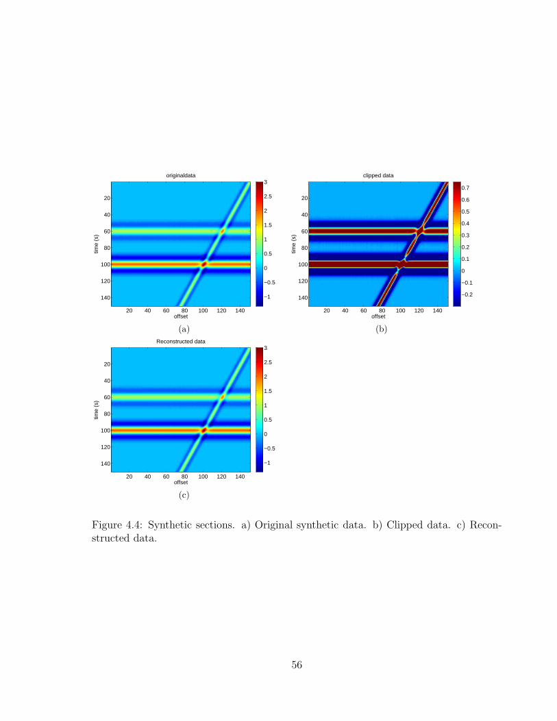
offset

time

(s)

originaldata

20 40 60 80 100 120 140

20

40

60

80

100

120

140 −1

−0.5

0

0.5

1

1.5

2

2.5

3

(a)

offset

time

(s)

clipped data

20 40 60 80 100 120 140

20

40

60

80

100

120

140 −0.2

−0.1

0

0.1

0.2

0.3

0.4

0.5

0.6

0.7

(b)

offset

time

(s)

Reconstructed data

20 40 60 80 100 120 140

20

40

60

80

100

120

140 −1

−0.5

0

0.5

1

1.5

2

2.5

3

(c)

Figure 4.4: Synthetic sections. a) Original synthetic data. b) Clipped data. c) Recon-structed data.

56

0 0.05 0.1 0.15−1

−0.5

0

0.5

1

1.5

2

time (s)

Am

plitu

de

(a)

0 0.05 0.1 0.15−0.4

−0.2

0

0.2

0.4

0.6

0.8

1

time(s)

Am

plitu

de

(b)

0 0.02 0.04 0.06 0.08 0.1 0.12 0.14 0.16−1

−0.5

0

0.5

1

1.5

2

time (s)

Am

plitu

de

SplineNFFT − POCS

(c)

Figure 4.5: a) Synthetic trace. b) Clipped trace. c) Reconstructed trace

57

another synthetic trace made up of two ricker wavelets. To test the algorithm data is

being clipped in Figure 4.5b. Followed by reconstruction using conventional spline and

NFFT POCS. NFFT POCS is able to restore the clipping perfectly where as spline gave

completely inaccurate reconstruction of second peak in Figure 4.5c.

4.3.2 Real data

The proposed reconstruction algorithm has been tested experimentally on the GPR data.

The data is acquired along an ice sheet. Snow and ice are ideal GPR media because their

stratification presents reflecting horizons with great continuity and interesting configu-

rations. Due to antenna-ground coupling or some other technical issue the amplitudes

in the acquired GPR data are clipped. They are clipped below −215 and above 215 − 1,

so there is no positive amplitude greater than 32767, and no negative amplitude below

-32768.

Figure 4.6 shows the GPR data with a lake bottom reflection. The sampling rate for

the acquired data set is 4ns. The bandwidth of data is 0-1250 MHz. Clipped amplitudes

are clearly visible in Figure 4.6 along the top horizon. The data is compromised of 300

traces, each sampled for 750 ns. Sample traces from the data set can be seen in Figure

4.7, where it is clearly evident that it is clipped with maximum amplitude of 32767 and

minimum amplitude of -32768.

The first step in commercial GPR processing software is the implementation of rub-

ber band interpolation (spline interpolation). Figure 4.8 shows the effectiveness of spline

interpolation for a GPR trace. Implementation of different interpolation technique on

GPR data is carried out. Cubic interpolation along with linear and nearest neighbour

interpolation is compared with spline interpolation. Cubic spline interpolation is im-

plemented on the trace, it is a piecewise third-order polynomial passing through set of

points. The result is not very effective with any other method except spline interpolation.

58

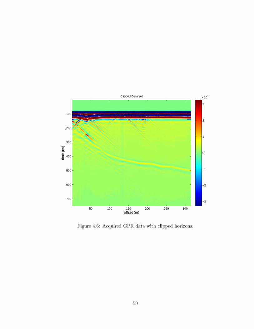
offset (m)

time

(ns)

Clipped Data set

50 100 150 200 250 300

100

200

300

400

500

600

700−3

−2

−1

0

1

2

3

x 104

Figure 4.6: Acquired GPR data with clipped horizons.

59

0 0.5 1 1.5 2 2.5 3

x 10−7

−4

−3

−2

−1

0

1

2

3

4x 10

4

time (ns)

Am

plitu

de

Original Clipped trace

Figure 4.7: Random extracted clipped trace from acquired GPR data.

60

−0.5 −0.45 −0.4 −0.35 −0.3 −0.25 −0.2 −0.15−2

−1.5

−1

−0.5

0

0.5

1x 10

5

Normalized time (sec)

Am

plitu

de

splinecubicnearest neighbourslinear

Figure 4.8: Comparative study for reconstruction of clipped amplitude

61

offset (m)

time

(ns)

spline Reconstructed data

50 100 150 200 250 300

100

200

300

400

500

600

700 −2

−1.5

−1

−0.5

0

0.5

1

1.5

x 105

Figure 4.9: Spline interpolation of clipped GPR data.

This effectiveness of spline interpolation makes it a favourite module in declipping or

desaturation for various GPR processing software. However, this method does not use

any information from the signal. The whole reconstruction procedure is based on the fact

that the interpolater is calculated on the basis of a few nearby data points. Figure 4.8,

in which spline is use for reconstruction of single trace from GPR data, shows relatively

good results as compared to other interpolators. Amplitudes are restored in Figure 4.9

on application of the spline based interpolation.

Effectiveness of modified POCS method is validated by comparing it with spline

interpolation on different GPR traces. Figure 4.10a shows that for the 10th trace, there

is difference in the reconstructed negative and positive clipping as compared to the spline

method. Figure 4.10b shows a difference in all four reconstructed clippings, these four

clips represent four different horizons. All of the clippings reconstructed have a significant

62

error in both negative and positive amplitudes. Figure 4.10b shows another trace, where

spline and Modified POCS give us similar results. Figure 4.10c and 4.11a also shows the

difference in reconstructed amplitudes.

63

−0.5 −0.45 −0.4 −0.35 −0.3 −0.25 −0.2 −0.15−1.5

−1

−0.5

0

0.5

1x 10

5

Normalized time (sec)

Am

plitu

de

clipped trace,NFFT − POCSspline

(a)

−0.5 −0.45 −0.4 −0.35 −0.3 −0.25 −0.2 −0.15−2

−1.5

−1

−0.5

0

0.5

1

1.5

2x 10

5

Normalized time (sec)

Am

plitu

de

clipped trace,NFFT − POCSspline

(b)

−0.5 −0.45 −0.4 −0.35 −0.3 −0.25 −0.2 −0.15−1.5

−1

−0.5

0

0.5

1

1.5x 10

5

Normalized time (sec)

Am

plitu

de

clipped trace,NFFT − POCSspline

(c)

Figure 4.10: Restored clipped amplitudes using Spline and Hybrid NFFT POCS. a) 10thtrace from restored GPR section. b) 30th trace from restored GPR section. c) 50th tracefrom restored GPR section.

Figure’s 4.11 and 4.12 shows that it is not always the case that Modified POCS

is constructing amplitudes smaller than the spline method. It can be seen in Figure

4.11a that the amplitude restored in the first clipping is higher compared to spline based

technique. Also, in Figure 4.11c, the restored clips have higher amplitude than the splines.

In Figure’s 4.10, 4.11 and 4.12 results obtain from our method differs from conventional

spline based method.

Figure 4.13 shows the reconstructed GPR section. Horizons are successfully recon-

structed, and the energy is continuous along the horizon, whereas the spline based re-

64

−0.5 −0.45 −0.4 −0.35 −0.3 −0.25 −0.2 −0.15−1.5

−1

−0.5

0

0.5

1x 10

5

Normalized time (sec)

Am

plitu

de

clipped trace,NFFT − POCSspline

(a)

−0.5 −0.45 −0.4 −0.35 −0.3 −0.25 −0.2 −0.15−2

−1.5

−1

−0.5

0

0.5

1x 10

5

Normalized time (sec)

Am

plitu

de

clipped trace,NFFT − POCSspline

(b)

−0.5 −0.45 −0.4 −0.35 −0.3 −0.25 −0.2 −0.15−2

−1.5

−1

−0.5

0

0.5

1x 10

5

Normalized time (sec)

Am

plitu

de

clipped trace,NFFT − POCSspline

(c)

Figure 4.11: Restored clipped amplitudes using Spline and Hybrid NFFT POCS. a) 100thtrace from restored GPR section. b) 150th trace from restored GPR section. c)b) 200thtrace from restored GPR section.

65

−0.5 −0.45 −0.4 −0.35 −0.3 −0.25 −0.2 −0.15−1.5

−1

−0.5

0

0.5

1x 10

5

Normalized time (sec)

Am

plitu

de

clipped trace,NFFT − POCSspline

(a)

−0.5 −0.45 −0.4 −0.35 −0.3 −0.25 −0.2 −0.15−1.5

−1

−0.5

0

0.5

1x 10

5

Normalized time (sec)

Am

plitu

de

clipped trace,NFFT − POCSspline

(b)

−0.5 −0.45 −0.4 −0.35 −0.3 −0.25 −0.2 −0.15−2

−1.5

−1

−0.5

0

0.5

1x 10

5

Normalized time (sec)

Am

plitu

de

clipped trace,NFFT − POCSspline

(c)

Figure 4.12: Restored clipped amplitudes using Spline and Hybrid NFFT POCS. a) 250thtrace from restored GPR section. b) 280th trace from restored GPR section. c)300thtrace from restored GPR section.

66

Reconstructed data

offset (m)

time

(ns)

50 100 150 200 250 300

100

200

300

400

500

600

700

−2

−1.5

−1

−0.5

0

0.5

1

1.5

x 105

Figure 4.13: Reconstructed data using Hybrid NFFT-POCS

constructed GPR section in Figure 4.9 seems to losing energy in the first and second

horizons. It is also noted in Figures 4.10, 4.11 and 4.12 that there is difference in re-

stored amplitudes from both the methods.

Residuals between original clipped GPR data and POCS based reconstruction is com-

puted. Figure 4.14 shows smoothness in the restored amplitudes across the horizons. The

first, second and third horizon shows constant lateral smoothness in reconstructed energy

across the horizons in each layer. The residual of original clipped data and spline based

method in Figure 4.15 shows that energy is not constant in the top horizons, which

indicates the drawback of spline interpolation. Figure 4.16 indicates difference in the

reconstructed horizons between Modified POCS and spline method, which reflects the

difference in the reconstructed data.

67

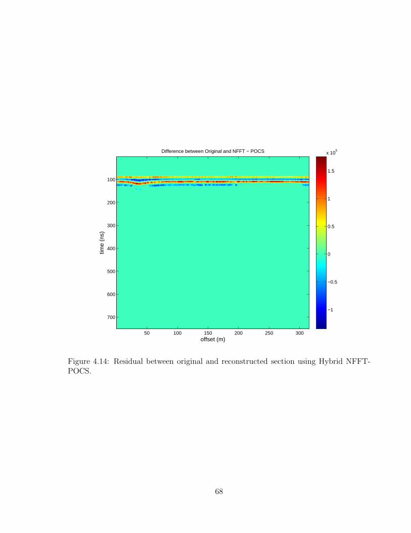
offset (m)

time

(ns)

Difference between Original and NFFT − POCS

50 100 150 200 250 300

100

200

300

400

500

600

700

−1

−0.5

0

0.5

1

1.5

x 105

Figure 4.14: Residual between original and reconstructed section using Hybrid NFFT-POCS.

68

offset (m)

time

(ns)

Difference between Original and Spline interpolation

50 100 150 200 250 300

100

200

300

400

500

600

700

−1

−0.5

0

0.5

1

1.5

x 105

Figure 4.15: Residual between original and reconstructed section using spline interpola-tion.

69

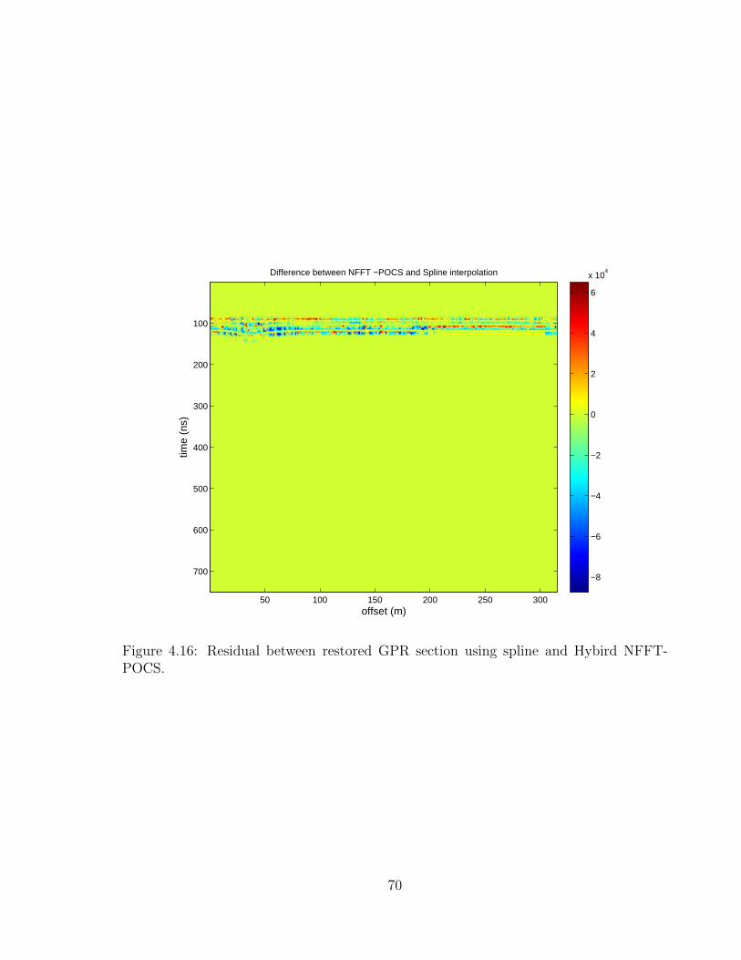
offset (m)

time

(ns)

Difference between NFFT −POCS and Spline interpolation

50 100 150 200 250 300

100

200

300

400

500

600

700−8

−6

−4

−2

0

2

4

6

x 104

Figure 4.16: Residual between restored GPR section using spline and Hybird NFFT-POCS.

70

4.4 Conclusion

In this chapter, an algorithm for clipped amplitude restoration using hybrid POCS has

been presented and tested. It is able to completely restore the clipped amplitudes of GPR

data. Two different methods for estimating the clipping have been tested. The first one

is conventional method of spline interpolation, which is largely adopted in GPR industry.

The second is hybrid POCS, which uses a priori information from the signal to recover

clipped amplitudes. A comparative study is done, which showed that Hybrid POCS is

better than conventional spline interpolation. Hybrid POCS is better technique due to

improved lateral continuity of the energy across the horizons in reconstructed data.

71

Chapter 5

Conclusion

This thesis studies the reconstruction of bandlimited seismic data using Fourier recon-

struction techniques. The main objective was to illustrate the use of Fourier reconstruc-

tion techniques of seismic data and to introduce Fourier method that provide robust and

efficient tools for seismic data reconstruction.

The main contributions of this thesis to the field of interpolation in geophysics can

be summerized as follows:

• Analysis of the presently available slow methodology, known as Adaptive Conjugate

Toeplitz (ACT) which uses simple DFT for reconstruction of missing samples in

regular and irregular data. This methodology gives good interpolation result, but

it is slow and inefficient (chapter 2).

• A novel reconstruction method called the Kaiser Bessel Non uniform Fast Fourier

Transform (NFFT). As the name suggest Kaiser Bessel NFFT is a convolution of

the Fast Fourier transform with a Kaiser Bessel filter. This methodology is tested

for both regular and irregular decimations. It allows the replacement of slow DFTs

with faster NFFTs (chapter 3).

• A problem of clipped amplitudes in GPR data has been solved. The problem of

restoring clipped amplitudes cannot be solved using simple techniques, due to the

presence of big gaps. A hybrid method is implemented which involves a combination

of NFFT with POCS (Projection on Convex Set). The declipping algorithm was

tested sucessfully with synthetic and real world examples. The results obtained

through this proposed hybrid methodology are better than conventional methods

72

like spline interpolation (chapter 4).

73

Bibliography

Abma, R., and Kabir, N., 2005, Comparison of interpolation algorithms: The Leading

Edge, 24, No. 10, 984–989.

Adorf, H. M., 1995, Interpolation of irregularly sampled data series – a survey: Astro-

nomical Data Analysis Software and Systems IV, 77, 460.

Bagaini, C., and Spagnolini, U., 1999, 2-d continuation operators and their applications:

Geophysics, 64, No. 2, 524–538.

Beylkin, G., Coifman, R., and Rokhlin, V., 1991, Fast wavelet transforms and numerical

algorithms: Comm. on Pure and Appl. Math., 44, 141–183.

Darche, G., 1990, Spatial interpolation using a fast parabolic transform: 60th Annual

International Meeting, SEG, Expanded Abstarcts, 1647–1650.

Duijndam, A. J. W., and Schonewille, M., 1999, Nonuniform fast fourier transform:

Geophysics, 64, 551.

Duijndam, A. J. W., Schonewille, M. A., and Hindriks, C. O. H., 1999, Reconstruction

of band-limited signals, irregularly sampled along one spatial direction: Geophysics,

64, No. 2, 524–538.

Dutt, A., and Rokhlin, V., 1993, Fast fourier transforms for nonequispaced data: SIAM

J. Sci. Comput., 14, No. 6, 1368–1393.

Feichtinger, H., Grochenig, K., and Strohmer, T., 1995a, Efficient numerical methods in

non-uniform sampling theory: Numerische Mathematik, 69, No. 4, 423–440.

Feichtinger, H. G., Grochenig, K., and Strohmer, T., 1995b, Efficient numerical methods

in non-uniform sampling theory: Numerische Mathematik, 69, 423–440.

74

Feng, X., and Sato, M., 2004, Prestack migration applied to gpr for lanmine detection:

Invrese problems, 20, 99–115.

Fomel, S., 2003, Seismic reflection data interpolation with differential offset and shot

continuation: Geophysics, 68, No. 2, 733–744.

Gazdag, J., 1978, Seismic migration problems and solutions: Geophysics, 43, 1342–1351.

Gerchberg, W., R, and Saxton, O., W, 1972, A practical algorithm for the determination

of phase from image and diffraction plane pictures: Optik, 35, 237–246.

Gulati, A., and Ferguson, R. J., 2010, Kaiser bessel gridding kernel for seismic data

regularization: CREWES Research Report, 22.

Hennenfent, G., and Herrmann, F. J., 2006a, Application of stable signal recovery to

seismic data interpolation: 76th Annual International Meeting, SEG, Expanded Ab-

starcts, 2797–2801.

Hennenfent, G., and Herrmann, F. J., 2006b, Seismic denoising with nonuniformly sam-

pled curvelets: IEEE Trans. on Computing in Science and Engineering, 8, No. 3,

16–25.

Hennenfent, G., and Herrmann, F. J., 2007, Random sampling: new insights into the re-

construction of coarsely-sampled wavefields: 77th Annual International Meeting, SEG,

Expanded Abstarcts, 2575–2579.

Hennenfent, G., and Herrmann, F. J., 2008, Simply denoise: Wavefield reconstruction

via jittered undersampling: Geophysics, 73, No. 3, V19–V28.

Hugonnet, P., and Canadas, G., 1995, Aliasing in the parabolic radon transform: SEG

Expanded Abstracts, 85, No. 1, 1366–1369.

75

Jackson, J. I., Meyer, C. H., Nishimura, D. G., and Macovski, A., 1991, Selection of a

convolution function for Fourier inversion using gridding [computerised tomography

application]: Medical Imaging, IEEE Transactions on, 10, No. 3, 473–478.

Keiner, J., Kunis, S., and Potts, D., 2008, Using nfft 3 – a software library for various

nonequispaced fast fourier transforms.

Knopp, T., Kunis, S., and Potts, D., 2007, A note on the iterative mri reconstruction

from nonuniform k-space data: Int. J. Biomed. Imag., 2007, Article ID 24,727, 9 pages.

Kunis, S., and Potts, D., 2005, Nfft2.0 user’s manual: available online at:

http://www.math.mu-luebeck.de/potts/nfft/, version 2, 1–22.

Lee, J., and Greengard, L., 2006, The type 3 nonuniform fft and its applications: Journal

of Computational Physics, 206, 1–5.

Liu, B., and Sacchi, M. D., 2004, Minimum weighted norm interpolation of seismic

records: Geophysics, 69, No. 6, 1560–1568.

Naghizadeh, M., and Sacchi, M. D., 2007a, Multistep autoregressive reconstruction of

seismic records: Geophysics, 72, No. 6, V111–V118.

Naghizadeh, M., and Sacchi, M. D., 2007b, Reconstruction of irregularly sampled, aliased

data with multistep autoregressive operators: SEG Technical Program Expanded Ab-

stracts, 26, 2580–2583.

Naghizadeh, M., and Sacchi, M. D., 2008a, Sampling functions and sparse reconstruction

methods: EAGE Conference, Rome, Italy.

Naghizadeh, M., and Sacchi, M. D., 2008b, Seismic data reconstruction using multidi-

mensional prediction filters: EAGE Conference, Rome, Italy.

76

Naghizadeh, M., and Sacchi, M. D., 2008c, Seismic trace interpolation using adaptive

prediction filters: CSEG Annual meeting.

Naghizadeh, M., and Sacchi, M. D., 2009a, Robust reconstruction of aliased data using

autoregressive spectral estimates: EAGE Conference, Amsterdam, Netherlands.

Naghizadeh, M., and Sacchi, M. D., 2009b, Sampling considerations for band-limited

fourier reconstruction of aliased seismic data: EAGE Conference, Amsterdam, Nether-

lands.

Naghizadeh, M., and Sacchi, M. D., 2010, Seismic data reconstruction using multidimen-

sional prediction filters: Geophysical Prospecting, 58, No. 2, 157–173.

Porsani, M., 1999, Seismic trace interpolation using half-step prediction filters: Geo-

physics, 64, No. 5, 1461–1467.

Ronen, J., 1987, Wave-equation trace interpolation: Geophysics, 52, No. 7, 973–984.

Sacchi, M., and Liu, B., 2005, Minimum weighted norm wavefield reconstruction for ava

imaging: Geophysical Prospecting, 53, No. 6, 787–801.

Sacchi, M. D., and Ulrych, T. J., 1996, Estimation of the discrete fourier transform, a

linear inversion approach: Geophysics, 61, No. 4, 1128–1136.

Sacchi, M. D., Ulrych, T. J., and Walker, C. J., 1998, Interpolation and extrapolation

using a high-resolution discrete fourier transform: IEEE Transaction on Signal Pro-

cessing, 46, No. 1, 31–38.

Schonewille, M., Klaedtke, A., Vigner, A., Brittan, J., and Martin, T., 2009, Seismic

data regularization with the anti-alias anti-leakage fourier transform: First Break, 27,

85–92.

77

Shewchuk, J. R., 1994, An introduction to the conjugate gradient method without the

agonizing pain, Tech. rep., Carnegie Mellon University, Pittsburgh, PA, USA.

Soubaras, R., 1994, Signal-preserving random noise attenuation by the f-x projection:

64th Annual International Meeting, SEG, Expanded Abstarcts, 1576–1579.

Spitz, S., 1991, Seismic trace interpolation in the F-X domain: Geophysics, 56, No. 6,

785–794.

Steidl, G., 1998, A note on fast fourier transforms for nonequispaced grids: Advances in

Computational Mathematics, 9, 337–352, 10.1023/A:1018901926283.

URL http://dx.doi.org/10.1023/A:1018901926283

Stolt, R. H., 2002, Seismic data mapping and reconstruction: Geophysics, 67, No. 3,

890–908.

Thorson, J. R., and Claerbout, J., 1985, Velocity-stack and slant-stack stochastic inver-

sion: Geophysics, 50, No. 6, 2727–2741.

Trad, D., 2003, Interpolation and multiple attenuation with migration operators: Geo-

physics, 68, No. 6, 2043–2054.

Trad, D., 2008, Five dimensional seismic data interpolation: 78th Annual International

Meeting, SEG, Expanded Abstarcts, 978–981.

Unser, M., 2000, Sampling - 50 years after shannon: Proceedings of the IEEE, 88, No. 4,

569–587.

Vermeer, G., 1990, Seismic wavefield sampling, vol. 4: Society of Exploration Geophysic-

sits, Tulsa, OK.

Verschuur, D. J., and Kabir, M. M. N., 1995, Restoration of missing offsets by parabolic

radon transform: Geophysical Prospecting, 43, No. 3, 347–368.

78

Vio, R., Strohmer, T., and Wamsteker, W., 2000, On the reconstruction of irregularly

sampled time series: Publications of the Astronomical Society of the Pacific, 112, 74

– 90.

Wiggins, R. A., and Miller, S. D., 1972, New noise-reduction technique applied to long-

period oscillations from the alaska earthquake: Bull. Seism. Soc. Am., 62, 471–479.

Xu, S., Zhang, Y., Pham, D., and Lambare, G., 2005, Antileakage fourier transform for

seismic data regularization: Geophysics, 70, No. 4, V87–V95.

79