Classification of Damage Signatures in Composite Plates · Classification of Damage Signatures in...

1

Classification of Damage Signatures in Composite Plates using One-Class SVMs12

Santanu Das Ashok N. Srivastava Aditi Chattopadhyay

Mechanical and Aerospace Eng. NASA Ames Research Center Mechanical and Aerospace Eng. ASU, Tempe, AZ 85287 Moffett Field, CA 94035 ASU, Tempe, AZ 85287 [email protected] [email protected] [email protected]

1 1 1-4244-0525-4/07/$20.00©2007 IEEE 2 The research is supported by Air Force Office of Scientific Research, grant number: F496200310174, technical monitor Dr. Clark Allred and NASA Ames Research Center, technical monitor Dr. A. N. Srivastava. Their support is gratefully acknowledged. This work has been accepted for publication in the Proceedings of the 2007 IEEE Aerospace Conference.

Abstract—Damage characterization through wave propagation and scattering is of considerable interest to many non-destructive evaluation techniques. For fiber-reinforced composites, complex waves can be generated during the tests due to the non-homogeneous and anisotropic nature of the material when compared to isotropic materials. Additional complexities are introduced due to the presence of the damage and thus results in difficulty to characterize these defects. The inability to detect damage in composite structures limits their use in practice. A major task of structural health monitoring is to identify and characterize the existing defects or defect evolution through the interactions between structural features and multidisciplinary physical phenomena. In a wave-based approach to addressing this problem, the presence of damage is characterized by the changes in the signature of the resultant wave that propagates through the structure. In order to measure and characterize the wave propagation, we use the response of the surface-mounted piezoelectric transducers as input to an advanced machine-learning based classifier known as a Support Vector Machine.

TABLE OF CONTENTS

1. INTRODUCTION......................................................1 2. EXISTING STATISTICAL CLASSIFIERS...................2 3. ONE-CLASS SVMS BASED CLASSIFIER ................3 4. CHOICE OF KERNEL PARAMETER ........................4 5. EXPERIMENTAL BACKGROUND ............................5 6. PREPROCESSING....................................................5 7. RESULTS AND DISCUSSIONS ..................................6 8. CONCLUSIONS .......................................................8 REFERENCES ...........................................................17 BIOGRAPHY .............................................................19

1. INTRODUCTION

We discuss an automated method of classifying sensor signals collected from different types of damage coupons to enable the detection and diagnosis of damage on composite structures using Support Vector Machines (SVMs), which are an advanced classification method from the field of machine learning. We use a special type of support vector machine known as the one-class SVMs as a pattern recognition tool for automatic anomaly detection and diagnosis on structures made from Carbon Fiber Reinforced Composite (CFRC) materials.

A key-step in the analysis of structural waveforms with the one-class SVM is transformation of the sensor signals into a joint time-frequency domain followed by statistical processing. Since the SVM results depend on the type of preprocessing method and the knowledge of kernel parameters, we evaluated the sensitivity of the classifier for different time-frequency based representations under the optimal setting of the kernel parameters. Our initial experiments indicate that one-class SVMs are capable of detecting and diagnosing certain structural failures on composite materials.

We also study the use of one-class SVMs to understand issues related to localized degradation of materials. Applying one-class SVMs to a lagged and windowed time-series representation of the wave propagation can help identify gradual degradation or subcomponent level changes in the structure. The proposed method is sensitive to certain changes in the vibration attributes and thus can be used as an indicator to ascertain the current status of the structure compared to its previous state. A second set of experiments have been conducted on bolted structure and the looseness of the bolted joint has been considered as a faulty situation.

2

The initial set of analysis indicates that the proposed technique can identify the gradual looseness of the bolt when subjected to different preload conditions.

The development of smart structures technology has coincided with the increased use of composite materials in structural design. Composite structures are becoming increasingly popular in both aerospace and other systems due to the benefit of reduced weight for given strength and stiffness requirements. However composite laminates have specific forms of damage that are not found in other materials, such as delamination, transverse matrix cracking, fiber fracture, and matrix cracking. Either one or combinations of these forms of damage may nucleate when the composite is subjected to fatigue, over-loading, low-velocity impact or under various test cases of drilled holes, notches, saw-cut and laminate stacking sequence mismatch. These forms of damage not only affect the way in which it responds to applied loads but also may lead to catastrophic failure of the structure under certain environmental condition. There are numerous reasons why it is desirable to ascertain the condition of a structure to determine if failure is imminent. For example, failure of a structure may result in loss of use which usually implies loss of revenue. In addition, repair costs resulting from the failure of a structure usually far exceed the cost of preventive maintenance repair. Moreover, failure of certain structures may result in collateral costs that could conceivably exceed the cost of the structure itself. Although failure of a structure may seem sudden to the uninformed observer, there frequently are numerous physical phenomena which precede catastrophic failure [3]. In order to perform preventive repairs it is necessary to not only look for these signatures, but to detect and interpret them. The exact location of the distress can be determined by employing multiple sensors. Fiber reinforced composite materials, in particular are very compatible to such diagnostic testing systems. Several techniques are being developed to detect, estimate and localize damage within a composite structure. A comprehensive literature review of damage detection and health monitoring methods for structural and mechanical systems was provided by Doebling, et al [30] and Chang [13, 14]. However, further research is necessary to obtain damage classification solutions to promote the use of composite materials in complex systems and the development of robust condition monitoring in hostile environments.

The overall objective of this research is to develop a robust technique for damage classification mainly in composite structures. The normal (zero-state) and abnormal attributes are extracted from the measured data of a structure and are further analyzed to characterize various states of the system. Once the diagnostic procedure is trained, subsequent test data can be examined to see if the features deviated from the normal behavior have significant similarity with certain abnormal attributes of the system. The use of SVMs to investigate the vibration signatures of damages in

composites has been demonstrated under various test applications.

Due to the time-varying nature of these signals, the time-frequency based method along with the Support Vector Machines algorithm has been used for their automatic classification purpose. The goal is to extract and classify the signature characteristics due to the presence of various types of defects in composite structures so that the status of the structure can be ascertained. The final effort is to evaluate the performance of the proposed classifier to investigate specific test cases like bolted joint in plate structure under different loading conditions.

When localized damage is induced in the structure, these distinct feature components are sensed by the neighboring transducers [4]. Extracting the featured components with suitable signal processing techniques is a major task in structural health monitoring (SHM). In the present research, characterization of sensor signals has been conducted to obtain the influence of defects on the structural response using the support vector machines (SVMs) technique.

The rest of the paper is organized in four sections. Section 2 provides a brief literature survey on the existing statistical classifiers. Section 3 recalls a brief description on the mathematical formulation of SVMs with some discussions on the high dimensional feature space. Section 4 describes some strategies on the choice of the parameters of the selected model and their influence on the SVMs classifier. Section 5 deals with the experimental details of the present research. Section 6 provides with some details on the preprocessing of the datasets. Section 7 presents the outcome of the classifier and gives some insight on the obtained results. Finally Section 8 summarizes the observations with some concluding remarks.

2. EXISTING STATISTICAL CLASSIFIERS

Several approaches exist for the identification of waveforms based on machine-learning techniques [5, 9, 22, 26, 28]. References [5] and [26] present examples of algorithms to analyze discrete and continuous data streams for outliers and possible anomalies. References [22, 28] describe methods that work on both discrete and continuous data streams, and [9] gives a method well-suited to analyzing continuous data streams. These systems either rely on having examples of failure signatures or rely on unsupervised learning techniques to characterize nominal behavior so that off-nominal behavior can be identified. A brief summary of the application of different pattern recognition techniques for structural health monitoring and damage detection is well documented in Los Alamos National Laboratory Report [1].

3

Figure 2: Geometric interpretation of optimal hyperplane construction for two-dimensional case.

In the first situation, we assume that we are given vibration signals that have already been classified by a human expert into m of n categories. These categories correspond to a failure mode. Then, we build a model such as a neural network, support vector machine, or a decision tree, that learns the relationship between the input vibration signals and the failure categories. This learning amounts to the estimation of a set of parameters of the model to maximize the classification accuracy. Once such a model is learned, when new vibration data is submitted to the model, it can predict (or classify) that vibration signal into the appropriate categories. Of course, due to the variation in the signal and other sources, the model performance may not be perfect. Nonetheless, this methodology works well for a variety of problems.

In many situations, however, we are not able to generate examples of all possible anomalies. In this case, we take a so-called unsupervised learning approach, where we learn the nominal behavior of the system only. When new data comes in, we compare it to what has been observed before. If it is sufficiently similar to previous observations, the system is characterized as operating in a nominal regime. Otherwise, it is said to be in an off-nominal situation.

3. ONE-CLASS SVMS BASED CLASSIFIER

The Support Vector Machine (SVM) provides non-linear approximations by mapping the input vectors into high dimensional feature spaces where a separating hyperplane is constructed. The idea behind this method is to map the n- dimensional vectors x of the input space X into a high-

dimensional (possibly infinite dimensional) feature space (figure.1). In this research, the input data is mapped into an infinite-dimensional feature space using a Radial Basis Function (RBF) kernel (equation 1). The dot product in the feature map (φ ) is implicitly computed by evaluating the simple kernel (K), thus avoiding the explicit calculation of the feature map.

( )⎟⎟⎟

⎠

⎞

⎜⎜⎜

⎝

⎛ −−>==< 2

2

2exp)(),(,

σφφ

ji

jiji

xxxxxxK

(1)

One class SVM belongs to a unique group of the SVM family where the training input vectors belong to one-class, i.e., the class representative of normal or nominal system behavior. The objective is to map the data into the feature space corresponding to the kernel and thereafter constructing the optimal hyperplane to separate the featured vectors from the origin with maximum margin. This process characterizes the nominal operation of the system in the feature space. All nominal points lie ‘above’ the optimal hyperplane, and it is assumed that all future nominal behavior will lie in the same region. The algorithm returns a decision function f(x) that evaluates for every new data point (x) to determine which side of the hyperplane it falls on in feature space. Figure 2 represents the schematic overview of the one-class SVM and its parameters. The maximum separation between the origin and the data point is obtained by solving the quadratic problem (equation 2). When this algorithm is applied to new data, the decision function is used to determine whether or not the data points lie above or below the hyperplane. Points that fall above the plane (away from the origin) are called, nominal, and other points are called anomalous.

Figure 1: Illustration of higher dimensional mapping for liner separation.

4

• Initialize model parameters: ν ,σ (range), training data points (x) • For eachσ , σ = minσ ,…, maxσ

- Solve dual problem to compute iα and ρ - Returns a decision f(x) on training points (x) - Plots classification curve - Compute optimal σ value

• Update kernel parameter σ • Solve dual problem to compute iα and ρ • Evaluate decision function f(y) on test points (y) • Output: Correct Classification rate and Outliers with scores

ρξνξρ

−∑=

+l

i ilww

bw 1

1,21

,,,min (2)

subject to ixw ξρφ −≥)(, , 0≥iξ , for ][ 1,0∈ν

where ν represents the upper bound on the fraction of the training error, ξ is the non-zero slack variable and ρ being the offset (figure 2). The target function in the dual problem can be written as,

),(21min

,jij

jii xxKαα

α∑ (3)

subject to ν

αli10 ≤≤ ,∑ =1iα

where iα represents the Lagrange’s multiplier. The

parameter ρ can be recovered for values of iα that satisfies the given constraints in equation (2) and the values of

)( ixφ for the corresponding iα are termed as support

vectors. The obtained iα and )( ixφ must satisfy the equation for the offset, expressed as,

∑=j

jij xxK ),(αρ (4)

The decision function for a given test vector )(yφ can be expressed in terms of the kernel as,

( ) ⎟⎠

⎞⎜⎝

⎛−= ∑

=

ραl

ijii xxKsignyf

1),( (5)

For the training data, the decision function takes the value of 1+ capturing most of the data points and 1− elsewhere. Once the dual problem (equation 3) is solved to obtain the support vectors, the optimal hyperplane is constructed in the feature space. For a new test point, the decision function evaluates which side of the hyperplane the given test point falls into, using equation 5. The steps of the adopted approach are shown in table 1.

4. CHOICE OF KERNEL PARAMETER

In order to design the One-Class SVMs classifier, we need to select appropriate kernel parameter σ for each class of data. The parameter σ controls the smoothness of the kernel function and is tuned based on the model

parameterν , such that the upper bound on the classification error is satisfied. There are several ways the parameter σ is tuned to adjust the kernel to obtain best possible results. In this research, the optimal value of the sigma selection is based on the approach proposed by Runar Unnthorsson [25]. In this approach, for a pre-assigned value of ν , the One-Class SVMs model is trained with a given set of data and the classification rate is plotted across a range of σ . This implies that the best possible classification accuracy that can be achieved is ( )ν−1 . The criteria for selecting the optimal σ is where the fraction of the correct classification

rate of the training data first touches the highest classification accuracy i.e. ( )ν−1 %, as demonstrated by the straight line in figure 3 where the x-axis and y-axis represents the σ variation and correct classification rate (in percentage) respectively. The choice of the model parameter ν is typically based on the assumption to set the highest allowable fraction of misclassification of the training data.

Figure 3: Demonstration of optimal σ selection X-axis: Variation of σ Y-axis: Classification rate (in percentage)

Table 1: One-Class SVMs Algorithm

5

In this work the value of ν is set to 0.05,implying that there would be 5% classification error on the training data as shown in figure 3.

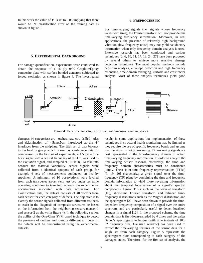
5. EXPERIMENTAL BACKGROUND

For damage quantification, experiments were conducted to obtain the response of a 16 ply 0/90 Graphite/Epoxy composite plate with surface bonded actuators subjected to forced excitation as shown in figure 4. The investigated

damages (4 categories) are notches, saw-cut, drilled holes and delamination of 4.5cmx5cm introduced at the 4th interfaces from the midplane. The fifth set of data belongs to the healthy group which is used as a reference data for comparison. In the first set of experiments, a 4.5 cycle tone burst signal with a central frequency of 8 KHz, was used as the excitation signal, and sampled at 100 KHz. To take into account the material variability, sensor signals were collected from 4 identical coupons of each group, for example 4 sets of measurements conducted on healthy specimen. A minimum of 10 observations were fetched from each transducer across each test bed under the same operating condition to take into account the experimental uncertainties associated with data acquisition. For classification data, the dataset consists of 40 vectors from each sensor for each category of defects. The objective is to classify the sensor signals collected from different test beds to assist in the diagnosis of composite structures be based on the information from the neighboring sensors (sensor-1 and sensor-2 as shown in figure 4). In the following section the ability of the One-Class SVM based technique to detect the presence of outliers and classify different attributes of the defects will be demonstrated using the experimental datasets.

6. PREPROCESSING

For time-varying signals (i.e. signals whose frequency varies with time), the Fourier transform will not provide this time-varying frequency information. Moreover, in real applications, the presence of relatively high background vibration (low frequency noise) may not yield satisfactory information when only frequency domain analysis is used. Extensive research has been conducted and various techniques [2, 6, 10, 11, 17, 18, 24, 27] have been proposed by several others to achieve more sensitive damage detection techniques. The most popular methods include cepstrum analysis, envelope detection and high frequency resonance, time-domain averaging, kurtosis and crest factor analysis. Most of these analysis techniques yield good

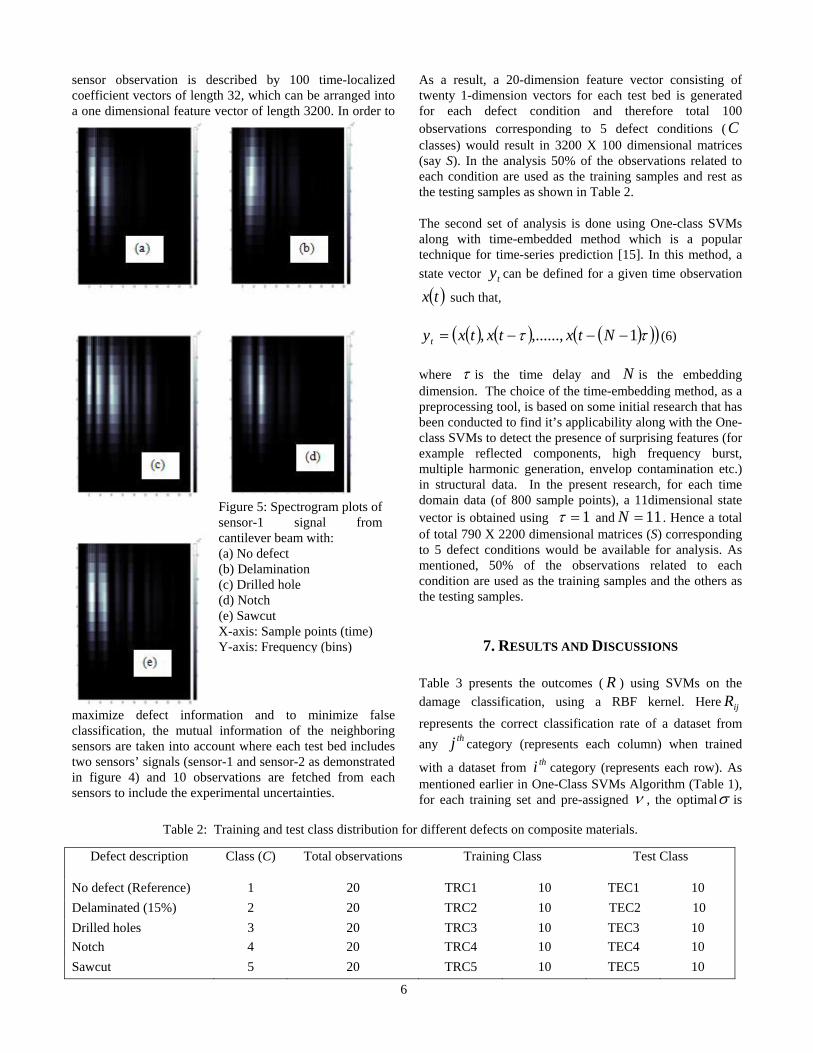
results in some applications but implementation of these techniques in structural health monitoring may be limited as they require the use of specific frequency bands and assume that the signal is not time-varying. Time-varying signals are best represented in the time-frequency domain to obtain time-varying frequency information. In order to analyze the time-varying sensor response effectively, the time and frequency domain characteristics must be considered jointly. These joint time-frequency representations (TFRs) [7, 19, 20] characterize a given signal over the time-frequency (TF) plane by combining the time and frequency domain information to yield more revealing information about the temporal localization of a signal’s spectral components. Linear TFRs such as the wavelet transform [16], short-time Fourier transform and bilinear time-frequency distributions such as the Wigner distribution and the spectrogram [29] have been shown to provide the time-dependent frequency composition of a signal over the entire spectrum, and are particularly useful to detect localized changes in a signal [12]. In the proposed scheme, the time domain data is first down-sampled by 4 times and thereafter Gabor’s spectrogram technique (with time instants of 100, 32 frequency bins, Gaussian window) has been used to extract the time-varying features of the sensor data for a single set from each category. Figure 5 represents the spectrogram plots corresponding to each category of the damaged states. Therefore, for the first set of analysis, the

Figure 4: Experimental setup with structural dimensions and interfaces

6

sensor observation is described by 100 time-localized coefficient vectors of length 32, which can be arranged into a one dimensional feature vector of length 3200. In order to

maximize defect information and to minimize false classification, the mutual information of the neighboring sensors are taken into account where each test bed includes two sensors’ signals (sensor-1 and sensor-2 as demonstrated in figure 4) and 10 observations are fetched from each sensors to include the experimental uncertainties.

As a result, a 20-dimension feature vector consisting of twenty 1-dimension vectors for each test bed is generated for each defect condition and therefore total 100 observations corresponding to 5 defect conditions ( C classes) would result in 3200 X 100 dimensional matrices (say S). In the analysis 50% of the observations related to each condition are used as the training samples and rest as the testing samples as shown in Table 2.

The second set of analysis is done using One-class SVMs along with time-embedded method which is a popular technique for time-series prediction [15]. In this method, a state vector ty can be defined for a given time observation

( )tx such that,

( ) ( ) ( )( )( )ττ 1,......,, −−−= Ntxtxtxyt (6)

where τ is the time delay and N is the embedding dimension. The choice of the time-embedding method, as a preprocessing tool, is based on some initial research that has been conducted to find it’s applicability along with the One-class SVMs to detect the presence of surprising features (for example reflected components, high frequency burst, multiple harmonic generation, envelop contamination etc.) in structural data. In the present research, for each time domain data (of 800 sample points), a 11dimensional state vector is obtained using 1=τ and 11=N . Hence a total of total 790 X 2200 dimensional matrices (S) corresponding to 5 defect conditions would be available for analysis. As mentioned, 50% of the observations related to each condition are used as the training samples and the others as the testing samples.

7. RESULTS AND DISCUSSIONS

Table 3 presents the outcomes ( R ) using SVMs on the damage classification, using a RBF kernel. Here ijR

represents the correct classification rate of a dataset from any thj category (represents each column) when trained

with a dataset from thi category (represents each row). As mentioned earlier in One-Class SVMs Algorithm (Table 1), for each training set and pre-assigned ν , the optimalσ is

Defect description Class (C) Total observations Training Class Test Class

No defect (Reference) 1 20 TRC1 10 TEC1 10 Delaminated (15%) 2 20 TRC2 10 TEC2 10 Drilled holes 3 20 TRC3 10 TEC3 10 Notch 4 20 TRC4 10 TEC4 10 Sawcut 5 20 TRC5 10 TEC5 10

Figure 5: Spectrogram plots of sensor-1 signal from cantilever beam with: (a) No defect (b) Delamination (c) Drilled hole (d) Notch (e) Sawcut X-axis: Sample points (time) Y-axis: Frequency (bins)

Table 2: Training and test class distribution for different defects on composite materials.

7

calculated and thereafter the dataset assigned for testing is being evaluated to compute the correct classification rate. In our current analysis, the ν is set to 0.05 and the optimal σ is being calculated for each training set. Once the matrix ( R ) is calculated, the selection criteria that two groups of signals belong to the same class is true when ijR and jiR

closely matches with higher classification rate i.e. jiij RR ≅ . When One-Class SVMs is trained

with thj category dataset, most of the thj category feature points lie on one side of the hyperplane but majority of the

thi category feature points (from test dataset) may or may not lie on the same side of the hyperplane. In case the category feature points don’t, then they are from different classes. However if they do, then it would be necessary to cross check if they both lie on the same side of the hyperplane, when the SVM is trained with category dataset instead. The geometrical interpretation for the selection criteria means that the two hyperplanes constructed individually by thi category and thj category dataset has to be very similar such that majority feature points from both the categories lie on the same side irrespective of the hyperplane constructed. In our present analysis, we set the selection criteria as ( )γ−≤− 105.0jiij RR , which

means that to belong to the same class the absolute difference of the correct classification rate obtained from two sets of data must be less than or equal to 5% of the maximum classification rate. Once the R matrix is obtained, a new matrix k

ijQ is formed for the thk sensor,

such that the following criteria hold,

If ( )γ−≤− 105.0jiij RR , 1== kji

kij QQ

Else 0== kji

kij QQ

(7)

For each sensor-1 (s1) and sensor-2 (s2), the kijQ is

evaluated and finally compared to obtain M , where

21 ss QQM I= (8)

The matrix ( M ) represents the final outcome of the classifier based on the mutual information of the sensor pairs and can infer that thi category and thj category

dataset belong to the same group, if 1== jiij MM .

Tables 3, 4 and 5 represents the set of analysis results (case-1) obtained using the first set of 3200 X 100 dimensional matrices with the time-frequency based features of the sensor data. The one-to-one classification rate for sensor-1

and sensor-2 are given in ijR matrix in table 3 and 4. Table

5 represents the outcome ( M ) using equation (7) and (8). It is worthwhile to mention that since the classifier is specifically not exclusively characterizing the changes in the signature, (healthy ~ defective), it would very often observe a majority of common attributes in a given dataset and therefore imposing selection criteria and mutual information (equation 7 & 8) from multiple sensors would minimize probable false classification. It is observed that the One-class Support Vector Machines algorithm correctly classifies class 1,2,3,5 but is unable to categorize the notch type defect.

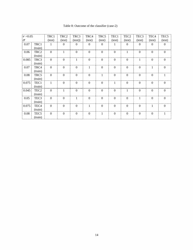
The analysis result (Case-2) for the dataset obtained from the time-embedding technique is shown in Tables 6, 7 and 8. The outcome indicates that the One-class SVMs with time-embedded technique has better classification performance for all defective states compared to the time-frequency based technique. One possible reason could be that the way the structural dataset is presented as a result of the preprocessing using time-embedded technique and thus enabling One-Class SVMs to separate these features in higher dimensional space. The final set of the classification analysis was conducted for a dataset collected from 2 identical coupons of each group to take into account the experimental and material uncertainties associated with data acquisition and manufacture respectively. A minimum of 20 vectors from each sensor for each category of defects were selected from a pool of 40 vectors and the selection was based on the two datasets having the closest distribution. In this effort, a total of total 790 X 4400 dimensional matrices (S) corresponding to 5 defect conditions has been used using time-embedded technique. The One-class SVMs classifiers successfully classified all the defect states, and are shown in table 9, 10 and 11(case-3). Throughout this research, the OSU SVM Classifier Matlab Toolbox (ver. 3.00) has been used for analysis purpose [http://svm.sourceforge.net/download.shtml].

A critical component in developing and implementing a robust diagnostics technique using guided wave is to acquire signals from distributed sensors and classify them. In the last decade, a significant amount of research has been conducted and major contributions have been made in the field of machine diagnostics and prognostics [10, 12, 17, 18, 21, 24]. Varma et. al. has proposed a time-frequency decomposition based technique to classify time-varying acoustic signals of reinforced concrete structures [7]. In this paper, the authors established the use to Matching Pursuit Decomposition (MPD) method as a pattern recognition tool and finally computed the classification rule based on the net contribution of the correlation coefficient information for the decomposed components from each class. The performance of the proposed classifier is indeed superior for signals having unlike patterns in time-frequency domain but shows some drop in the probability of correct classification as the time-frequency patterns gets similar (refer [7] – page

8

0.4

0.5

0.6

0.7

0.8

0.9

1

30 40 50 60 70 80 90100

4). Michaels et. al [19] conducted a comparative study on the performances feature-based-classifiers and demonstrated some applications in the SHM and NDE, using wave based technique. In this paper, the author adopted a differential scheme (normal ~ abnormal), to compute the features in time, frequency or joint time-frequency domain and examined the similarity measurement using Fisher Discriminant Ratio (FDR). One of the major conclusions made by the author is that the classifier performance improves significantly with multiple input feature vectors, when compared to a single input. Our present work provides a One-Class based classification technique using feature vectors extracted applying the spectrogram and time-embedding method directly to the sensor response but not the difference output. It has been demonstrated that the developed analysis based on mutual information from multiple sensor is an effective way of minimizing the possibility of false classification, when coupled with a selection criterion.

The final investigation was conducted to characterize sub-component level degradation of systems. In our current effort, the effect of the presence of a bolt in the plate with different levels of applied torque is investigated using experimental datasets. Experiments are conducted on a 38 x 38 x 0.15875cm aluminum cantilever plate with surface bonded transducers is used and the response near the bolted joint is recorded for various applied torque values.

These torque settings were achieved using a torque wrench in increments of 20 in-lb from 35 (minimum) to 80 (maximum) in-lb and the torque range is based on the tolerance of the bolt. The actuator and the sensors are placed at a distance of 2.5cms and 10cms from the center of the bolt respectively, in the radial direction as shown in figure 6. The actuator is subjected to a 4.5 cycle tone burst

signal with a central frequency of 8 KHz, was used as the excitation signal, and sampled at 100 KHz. Initially all bolts were kept tightened at maximum allowable torque i.e. 85 in-lb, represented as 100 percentage or full torque. Figure 7

demonstrates the application of One-Class SVMs to the time-embedded representation of the sensor-1 to identify the gradual changes in torque level at bolt-1 and thus defining the state of the structure under different loading conditions.

8. CONCLUSIONS

A wave based approach is used to characterize different defect states in composite laminates in terms of the changes in the signature of the resultant wave that propagates through the anisotropic medium. The current effort demonstrates the use of “One-Class SVMs” technique as a signal processing tool to demonstrate damage classification technique based on time-frequency information. Furthermore, it has also been demonstrated that using time-embedded technique with “One-Class SVMs” can lead to better classification in the presence of material and experimental uncertainties. Further research will be conducted to address some issues to increase the robustness of the current model in the presence of material uncertainties. Another area of future work is to use one-class SVMs to characterize damage signatures where we assume that there are no labeled nominal examples. In this case, we would assume that we only have a set of examples, some of which are nominal, and some of which are off-nominal. The methodology outlined in this paper may be useful in separating these two cases, thus enabling analysis of systems which don’t have labeled examples.

Figure 6: Experimental setup for a bolted joint structure

Figure 7: Illustration of gradual changes in torque level at bolt-1 X-axis: Variation of torque level (in percentage) Y-axis: Classification rate

9

ijR ν =0.05 σ

TRC1 (test)

TRC2 (test)

TRC3 (test))

TRC4 (test)

TRC5 (test)

TEC1 (test)

TEC2 (test)

TEC3 (test)

TEC4 (test)

TEC5 (test)

0.003 TRC1 (train)

0.951 0.7863 0.7196 0.7210 0.6776 0.8943 0.792 0.744 0.6671 0.6663

0.004 TRC2 (train)

0.9265 0.9501 0.826 0.8283 0.766 0.9396 0.8941 0.8535 0.7826 0.7291

0.005 TRC3 (train)

0.8950 0.8405 0.9528 0.8466 0.7425 0.9135 0.8671 0.8801 0.7780 0.7330

0.007 TRC4 (train)

0.919 0.8746 0.8813 0.9506 0.7733 0.9255 0.9148 0.9053 0.8680 0.7661

0.008 TRC5 (train)

0.9356 0.8761 0.8745 0.8435 0.9503 0.9340 0.8940 0.8556 0.7811 0.7665

0..003 TEC1 (train)

0.8756 0.7951 0.7311 0.7181 0.6598 0.9536 0.8098 0.7406 0.6688 0.6785

0.007 TEC2 (train)

0.9166 0.8910 0.8651 0.8738 0.7845 0.9323 0.9508 0.9026 0.8205 0.7681

0.005 TEC3 (train)

0.8838 0.816 0.8380 0.8146 0.727 0.8886 0.8458 0.9121 0.7708 0.7101

0.008 TEC4 (train)

0.9301 0.9033 0.8875 0.945 0.8013 0.9416 0.929 0.9113 0.9516 0.7940

0.007 TEC5 (train)

0.905 0.8728 0.8531 0.8393 0.7843 0.9226 0.8963 0.8618 0.8081 0.9531

Table 3: Classification rate ( ijR matrix) for sensor-1 (case-1)

10


ijR ν =0.05 σ

TRC1 (test)

TRC2 (test)

TRC3 (test))

TRC4 (test)

TRC5 (test)

TEC1 (test)

TEC2 (test)

TEC3 (test)

TEC4 (test)

TEC5 (test)

0.003 TRC1 (train)

0.951 0.7863 0.7196 0.7210 0.6776 0.8943 0.792 0.744 0.6671 0.6663

0.004 TRC2 (train)

0.9265 0.9501 0.826 0.8283 0.766 0.9396 0.8941 0.8535 0.7826 0.7291

0.005 TRC3 (train)

0.8950 0.8405 0.9528 0.8466 0.7425 0.9135 0.8671 0.8801 0.7780 0.7330

0.007 TRC4 (train)

0.919 0.8746 0.8813 0.9506 0.7733 0.9255 0.9148 0.9053 0.8680 0.7661

0.008 TRC5 (train)

0.9356 0.8761 0.8745 0.8435 0.9503 0.9340 0.8940 0.8556 0.7811 0.7665

0..003 TEC1 (train)

0.8756 0.7951 0.7311 0.7181 0.6598 0.9536 0.8098 0.7406 0.6688 0.6785

0.007 TEC2 (train)

0.9166 0.8910 0.8651 0.8738 0.7845 0.9323 0.9508 0.9026 0.8205 0.7681

0.005 TEC3 (train)

0.8838 0.816 0.8380 0.8146 0.727 0.8886 0.8458 0.9121 0.7708 0.7101

0.008 TEC4 (train)

0.9301 0.9033 0.8875 0.945 0.8013 0.9416 0.929 0.9113 0.9516 0.7940

0.007 TEC5 (train)

0.905 0.8728 0.8531 0.8393 0.7843 0.9226 0.8963 0.8618 0.8081 0.9531

11

Table 5: Outcome of the classifier (case-1)

ijM TRC1 (test)

TRC2 (test)

TRC3(test))

TRC4(test)

TRC5(test)

TEC1(test)

TEC2(test)

TEC3(test)

TEC4 (test)

TEC5 (test)

TRC1 (train)

1 0 0 0 0 1 0 0 0 0 TRC2 (train)

0 1 0 0 0 0 1 0 0 0 TRC3 (train)

0 0 1 0 0 0 0 1 0 0 TRC4 (train)

0 0 0 1 0 0 0 0 0 0 TRC5 (train)

0 0 0 0 1 0 0 0 0 1 TEC1 (train)

1 0 0 0 0 1 0 0 0 0 TEC2 (train)

0 1 0 0 0 0 1 0 0 0 TEC3 (train)

0 0 1 0 0 0 0 1 0 0 TEC4 (train)

0 0 0 0 0 0 0 0 1 0 TEC5 (train)

0 0 0 0 1 0 0 0 0 1

12

ν =0.05 σ

TRC1 (test)

TRC2 (test)

TRC3 (test))

TRC4 (test)

TRC5 (test)

TEC1 (test)

TEC2 (test)

TEC3 (test)

TEC4 (test)

TEC5 (test)

0.05 TRC1 (train)

0.9531 0.8367 0.8063 0.8012 0.7519 0.9265 0.8291 0.8038 0.7873 0.7519

0.055 TRC2 (train)

0.9696 0.9531 0.8645 0.9367 0.8341 0.9696 0.9278 0.8645 0.9417 0.8544

0.075 TRC3 (train)

0.9835 0.9341 0.9506 0.9746 0.9126 0.9810 0.9468 0.9354 0.9569 0.9189

0.07 TRC4 (train)

0.9696 0.8898 0.8645 0.9531 0.8329 0.9696 0.8860 0.8683 0.9341 0.8367

0.07 TRC5 (train)

1 0.9468 0.9354 0.9911 0.9519 1 0.9493 0.9392 0.9886 0.9227

0.055 TEC1 (train)

0.9493 0.8506 0.8316 0.8683 0.7949 0.9531 0.8417 0.8316 0.8443 0.7987

0.06 TEC2 (train)

0.9658 0.9215 0.8835 0.9506 0.8759 0.9645 0.9506 0.8810 0.9405 0.8835

0.085 TEC3 (train)

0.9974 0.9455 0.9341 0.9924 0.9227 0.9962 0.9493 0.9531 0.9860 0.9291

0.055 TEC4 (train)

0.967 0.8797 0.8746 0.9582 0.8240 0.9632 0.8810 0.8784 0.9531 0.8291

0.075 TEC5 (train)

1 0.9569 0.9405 0.9949 0.9253 1 0.9594 0.9468 0.9949 0.9519


13

ν =0.05 σ

TRC1 (test)

TRC2 (test)

TRC3 (test))

TRC4 (test)

TRC5 (test)

TEC1 (test)

TEC2 (test)

TEC3 (test)

TEC4 (test)

TEC5 (test)

0.07 TRC1 (train)

0.9519 0.9544 0.8873 0.9227 0.9075 0.9430 0.9557 0.8898 0.9126 0.9088

0.06 TRC2 (train)

0.8974 0.9519 0.8443 0.9050 0.8974 0.9000 0.9417 0.8519 0.8924 0.9012

0.085 TRC3 (train)

0.9670 0.9519 0.9519 0.7557 0.9075 0.9683 0.9569 0.9468 0.7189 0.9025

0.07 TRC4 (train)

0.9582 0.9873 0.8987 0.9544 0.9177 0.9607 0.9949 0.9088 0.9342 0.9113

0.08 TRC5 (train)

0.9405 0.9594 0.9569 0.9177 0.9506 0.9468 0.9594 0.9544 0.8974 0.9506

0.075 TEC1 (train)

0.9430 0.9594 0.8898 0.9265 0.9101 0.9506 0.9594 0.8924 0.9189 0.9012

0.045 TEC2 (train)

0.8126 0.9227 0.8417 0.8113 0.8746 0.8253 0.9531 0.8329 0.8025 0.8772

0.05 TEC3 (train)

0.9506 0.9354 0.9189 0.7708 0.8962 0.9443 0.9367 0.9506 0.7240 0.9000

0.075 TEC4 (train)

0.9594 0.9936 0.9050 0.9468 0.9202 0.9620 0.9987 0.9063 0.9582 0.9202

0.08 TEC5 (train)

0.9493 0.9594 0.9544 0.9215 0.9354 0.9506 0.9569 0.9594 0.9113 0.9531


14


ν =0.05 σ

TRC1 (test)

TRC2 (test)

TRC3 (test))

TRC4 (test)

TRC5 (test)

TEC1 (test)

TEC2 (test)

TEC3 (test)

TEC4 (test)

TEC5 (test)

0.07 TRC1 (train)

1 0 0 0 0 1 0 0 0 0

0.06 TRC2 (train)

0 1 0 0 0 0 1 0 0 0

0.085 TRC3 (train)

0 0 1 0 0 0 0 1 0 0

0.07 TRC4 (train)

0 0 0 1 0 0 0 0 1 0

0.08 TRC5 (train)

0 0 0 0 1 0 0 0 0 1

0.075 TEC1 (train)

1 0 0 0 0 1 0 0 0 0

0.045 TEC2 (train)

0 1 0 0 0 0 1 0 0 0

0.05 TEC3 (train)

0 0 1 0 0 0 0 1 0 0

0.075 TEC4 (train)

0 0 0 1 0 0 0 0 1 0

0.08 TEC5 (train)

0 0 0 0 1 0 0 0 0 1

15

ν =0.05 σ

TRC1 (test)

TRC2 (test)

TRC3 (test))

TRC4 (test)

TRC5 (test)

TEC1 (test)

TEC2 (test)

TEC3 (test)

TEC4 (test)

TEC5 (test)

0.055 TRC1 (train)

0.9544 0.6873 0.8683 0.6227 0.8101 0.7620 0.6278 0.8075 0.4949 0.7202

0.16 TRC2 (train)

0.9594 0.9506 0.8468 0.7860 0.8202 0.9177 0.7683 0.8696 0.7911 0.8202

0.105 TRC3 (train)

0.9164 0.7189 0.9506 0.6519 0.8278 0.8797 0.7012 0.8594 0.6443 0.8240

0.08 TRC4 (train)

0.8468 0.8075 0.8632 0.9531 0.8215 0.9025 0.7025 0.8455 0.6734 0.8139

0.09 TRC5 (train)

0.8797 0.6974 0.9050 0.6607 0.9557 0.8822 0.7025 0.9139 0.5962 0.9038

0.06 TEC1 (train)

0.8012 0.6506 0.8506 0.5379 0.7569 0.9544 0.6924 0.8670 0.6468 0.8278

0.155 TEC2 (train)

0.9126 0.7620 0.8670 0.7924 0.8189 0.9594 0.9531 0.8455 0.7860 0.8215

0.115 TEC3 (train)

0.9038 0.7202 0.8835 0.6835 0.8379 0.9405 0.7303 0.9519 0.6658 0.8303

0.075 TEC4 (train)

0.8822 0.6974 0.8405 0.6645 0.8025 0.8519 0.8063 0.8519 0.9544 0.8050

0.085 TEC5 (train)

0.8278 0.6873 0.9025 0.5784 0.9038 0.8721 0.6797 0.8936 0.6177 0.9544


16

ν =0.05 σ

TRC1 (test)

TRC2 (test)

TRC3 (test))

TRC4 (test)

TRC5 (test)

TEC1 (test)

TEC2 (test)

TEC3 (test)

TEC4 (test)

TEC5 (test)

0.115 TRC1 (train)

0.9519 0.9291 0.8949 0.7936 0.9202 0.9240 0.9113 0.8949 0.8012 0.9240

0.08 TRC2 (train)

0.6658 0.9506 0.6215 0.7151 0.6683 0.6379 0.8620 0.6924 0.6582 0.6063

0.1 TRC3 (train)

0.8392 0.8645 0.9531 0.7164 0.8569 0.8341 0.8860 0.8392 0.6734 0.8506

0.1 TRC4 (train)

0.8835 0.9126 0.8075 0.9544 0.8848 0.7987 0.9075 0.7949 0.7379 0.8557

0.12 TRC5 (train)

0.8493 0.8873 0.8670 0.7367 0.9506 0.8873 0.8873 0.8746 0.7215 0.8911

0.115 TEC1 (train)

0.9177 0.9063 0.8962 0.8139 0.9240 0.9531 0.9227 0.8949 0.7974 0.9202

0.08 TEC2 (train)

0.6353 0.8594 0.6886 0.6557 0.6088 0.6594 0.9557 0.6139 0.7126 0.6645

0.095 TEC3 (train)

0.8240 0.8746 0.8341 0.6582 0.8544 0.8519 0.8670 0.9506 0.7101 0.8493

0.11 TEC4 (train)

0.8139 0.9088 0.7962 0.7582 0.8721 0.8987 0.9202 0.8215 0.9557 0.8848

0.12 TEC5 (train)

0.8417 0.8873 0.8734 0.7265 0.8911 0.8683 0.8873 0.8645 0.7341 0.9531


17


REFERENCES

[1] A Review of Structural Health Monitoring Literature: 1996-2001. Los Alamos National Laboratory Report, LA-13976-MS, 2003.

[2] A. Barkov, N. Barkova and J. S. Mitchell “Condition Assessment and Life Prediction of Rolling Element Bearings Part. 1,” Sound Vibr, Vol. 29: 10-17, 1999.

[3] A. Chattopadhyay, S. Das and A. Papandreou-Suppappola, “Structural Health Monitoring of Composites using Wave Based Technique and Novel Signal processing,” Condition Monitoring, King’s College, Cambridge, United Kingdom, 2005.

[4] A. Chattopadhyay, S. Das and A. Papandreou-Suppappola, “A Novel Signal Processing Technique for Damage Detection in Composites,” International Conference on Computational and Experimental Engineering & Sciences, India, 2005.

[5] A. N. Srivastava, “Discovering Anomalies in Sequences with Applications to System Health,” Proceedings of the 2005 Joint Army Navy NASA Air Force Interagency Conference on Propulsion, Charleston SC, 2005.

Nu=0.95

TRC1 (test)

TRC2 (test)

TRC3 (test))

TRC4 (test)

TRC5 (test)

TEC1 (test)

TEC2 (test)

TEC3 (test)

TEC4 (test)

TEC5 (test)

0.07 TRC1 (train)

1 0 0 0 0 1 0 0 0 0

0.06 TRC2 (train)

0 1 0 0 0 0 1 0 0 0

0.085 TRC3 (train)

0 0 1 0 0 0 0 1 0 0

0.07 TRC4 (train)

0 0 0 1 0 0 0 0 1 0

0.08 TRC5 (train)

0 0 0 0 1 0 0 0 0 1

0.075 TEC1 (train)

1 0 0 0 0 1 0 0 0 0

0.045 TEC2 (train)

0 1 0 0 0 0 1 0 0 0

0.05 TEC3 (train)

0 0 1 0 0 0 0 1 0 0

0.075 TEC4 (train)

0 0 0 1 0 0 0 0 1 0

0.08 TEC5 (train)

0 0 0 0 1 0 0 0 0 1

18

[6]A. Papandreou-Suppappola and S. B. Suppappola, "Analysis and classification of time-varying signals with multiple time-frequency structures,'' IEEE Signal Processing Letters, vol. 9, 92-95, March 2002.

[7] S. Pon Varma, A. Papandreou-Suppappola, and S. B. Suppappola “Detecting faults in structures using time-frequency techniques,” International Conference on Acoustics, Speech, and Signal Processing, vol. 6, pp. 3593-3596, 2001.

[8]B. Samanta, R. Khamis, Al-Balushi. and Saeed A. Al-Araimi., “Bearing Fault Detection Using Artificial Neural Networks and Genetic Algorithm,” EURASIP Journal on Applied Signal Processing, Vol. 2004(3): 366-377, 2004.

[9] D. L. Iverson. “Inductive System Health Monitoring,” Proceedings of the International Conference on Artificial Intelligence, Vol. 2, June 21-24, 2004.

[10] D. Dyer and R. M. Stewart, “Detection of Rolling Element Bearing Damage by Statistical Vibration Analysis,” ASME Trans Mech Des, Vol. 100: 229-35, 1978.

[11] D. R. Harting, “Demodulated Resonance Analysis: a Powerful Incipient Failure Detection Technique,” ISA Trans, Vol. 17: 35-40. 1978.

[12] F. He and W. Shi, “WPT-SVMs based approach for fault detection of valves in reciprocating pumps,” Proceedings of the American Control Conference AK, Vol. 6, 4566-4570, 2002.

[13] F. K. Chang, ed. Structural Health Monitoring: Current Status and Perspectives, Proceedings of the International Workshop on Structural Health Monitoring, Stanford University, 1997.

[14] F. K. Chang, (Editor), Structural Health Monitoring, Proceedings of the 2nd International Workshop on Structural Health Monitoring, Stanford University, Stanford, CA, 1999.

[15] F. Perez-Cruz and O. Bousquet, “Kernel methods and their potential use in signal processing,” Signal Processing Magazine, IEEE, Vol. 21(3):57-65, May 2004.

[16]G. Devuyst et.al, “Automatic Classification of HITS into Artifacts or Solid or Gaseous Emboli by a Wavelet Representation Combined with Dual-Gate TCD,” American Heart Association, Inc., Vol. 32: 2803-2809, 2001.

[17] H. Prasad, M. Ghosh and S. Biswas, “Diagnostic Monitoring of Rolling Element Bearings by High Frequency Resonance Technique,” ASLE Trans, Vol. 28:439-448, 1985.

[18]J. Lei, “Failure Detection of Bearings,” Xi’an: Jiaotong University Press, 1988.

[19]J. Michaels, A. Cobb, and T. Michaels, “A comparison of feature-based classifiers for ultrasonic structural health monitoring,” Health Monitoring and Smart Nondestructive Evaluation of Structural and Biological Systems III, Proceedings of the SPIE, Volume 5394, pp. 363-374, 2004.

[20] L. Cohen “Time-Frequency Analysis,” Prentice-Hall, Englewood Cliffs, NJ, 1995.

[21] M. Lebold, K. McClintic, R. Campbell, C. Byingtonand and K. Maynard, “Review Of Vibration Analysis Methods for Gearbox Diagnostics and Prognostics,” Proceedings of the 54th Meeting of the Society for Machinery Failure Prevention Technology, Virginia Beach, VA, 623-634, 2000.

[22] M. Schwabacher, “Machine learning for rocket propulsion health monitoring,” Proceedings of the Society of Automotive Engineers World Aerospace Congress, 114-1, Dallas, Texas, 2005.

[23] P. L. Rosin, H. O. Nyongesa, and A. W. Otieno "Classification of Delaminated Composites using Neuro-Fuzzy Image Analysis", 6th UK Workshop on Fuzzy Systems, 267-273, Uxbridge, 1999.

[24] P. D. McFadden and J. D Smith, “Vibration Monitoring of Rolling Element Bearings by High Frequency Resonance Technique-a review,” Tribology Int, Vol. 17: 3-10, 1984.

[25] R. Unnthorsson, R. T. Runarsson and T. M. Johnson, “Model selection in one class nu-SVMs using RBF kernels,” 16th conference on Condition Monitoring and Diagnostic Engineering Management, 27-29 August 2003.

[26] S. Budalakoti, A. N. Srivastava and R. Akella, “Discovering Atypical Flights in Sequences of Discrete Flight Parameters,” accepted for publication in the Proceedings of the IEEE Aerospace Conference, 2006.

[27] S. Braun and B. Datner, “Analysis of Roller/Ball Bearing Vibrations,” ASME Trans Mech Des, Vol.101: 118-25, 1979.

19

[28] S. D. Bay and M. Schwabacher, “Mining Distance-Based Outliers in Near Linear Time with Randomization and a Simple Pruning Rule,” Proceedings of the Ninth ACM SIGKDD International Conference on Knowledge Discovery and Data Mining, 2003.

[29] S. P. Ebenezer, A. Papandreou-Suppappola, and S. Suppappola, ``Classification of acoustic emissions using time-frequency techniques,'' accepted for publication, EURASIP Journal on Applied Signal Processing, 2003.

[30] S. W. Doebling, C. R. Farrar, M.B. Prime and D.W. Shevitz, "Damage Identification and Health Monitoring of Structural and Mechanical Systems from Changes in Their Vibration Characteristics: a Literature Review," Los Alamos National Laboratory, Report LA-13070-MS, 1996.

BIOGRAPHY

Santanu Das received his B.E. degree in Electrical engineering from JGEC, India and M.S. Degrees degree in Microsystems engineering from University of Applied Sciences, furtwangen, Germany. After his masters’ degree, he started working for European Aeronautics Defense and Space Company (EADS), Munich, Germany. He is currently a graduate student at the Department of Mechanical and Aerospace Engineering at Arizona State University. His research focuses on structural health monitoring for heterogeneous structures. Other research interests include application-specific signal processing and circuit design.

Ashok N. Srivastava, Ph.D. is the leader of the Intelligent Data Understanding group at NASA Ames Research Center. The group performs research and development of advanced machine learning and data mining algorithms in support of NASA missions. He is the lead researcher for numerous programs at NASA, including those involved with improving aviation safety, development of new technologies to improve the safety of next generation propulsion systems, fundamental studies in the

earth sciences to understand climate change, and studies in astrophysics regarding the large-scale structure of the universe. He has won numerous awards, including the NASA Distinguished Performance Award, NASA Group Achievement Awards, the IBM Golden Circle Award, the Department of Education Merit Fellowship, and several fellowships from the University of Colorado. Ashok holds a Ph.D. in Electrical Engineering from the University of Colorado at Boulder.

Aditi Chattopadhyay, Ph.D. is a professor of mechanical and aerospace engineering at Arizona State University whose career spans over 20 years. Chattopadhyay is recognized internationally for her contributions in a variety of multidisciplinary areas, such as smart structures and materials, composites, rotary wing dynamics, and multidisciplinary design optimization. She has published more than 30 archival journal papers and over 130 other refereed publications. Chattopadhyay is an associate editor of AIAA's journal, Inverse Problems in Engineering and Engineering Optimization. She was the recipient of several academic, research, and best paper awards. She was inducted into the Georgia Tech Hall of Fame and earned the Outstanding Engineering Alumni Award in 1995. She received the Faculty Achievement Award for Excellence in Research from Arizona State in 2000. She is a Fellow of AIAA and ASME.

Classification of Damage Signatures in Composite Plates · Classification of Damage Signatures in...

Documents

Transcript of Classification of Damage Signatures in Composite Plates · Classification of Damage Signatures in...