Classification: Decision Trees, and Naïve Bayes etc. March 17, 2010 Adapted from Chapters 4 and 5...
53
Classification: Decision Trees, and Naïve Bayes etc. March 17, 2010 Adapted from Chapters 4 and 5 of the book Introduction to Data Mining by Tan, Steinbach, Kumar
-
Upload
jeremy-skinner -
Category
Documents
-
view
217 -
download
1
Transcript of Classification: Decision Trees, and Naïve Bayes etc. March 17, 2010 Adapted from Chapters 4 and 5...

Classification: Decision Trees, and Naïve Bayes etc.
March 17, 2010
Adapted from Chapters 4 and 5 of the bookIntroduction to Data Mining
byTan, Steinbach, Kumar

Classification: Definition
Given a collection of records (training set )– Each record contains a set of attributes, one of
the attributes is the class. Find a model for class attribute as a
function of the values of other attributes. Goal: previously unseen records should be
assigned a class as accurately as possible.– A test set is used to determine the accuracy of
the model. Usually, the given data set is divided into training and test sets, with training set used to build the model and test set used to validate it.

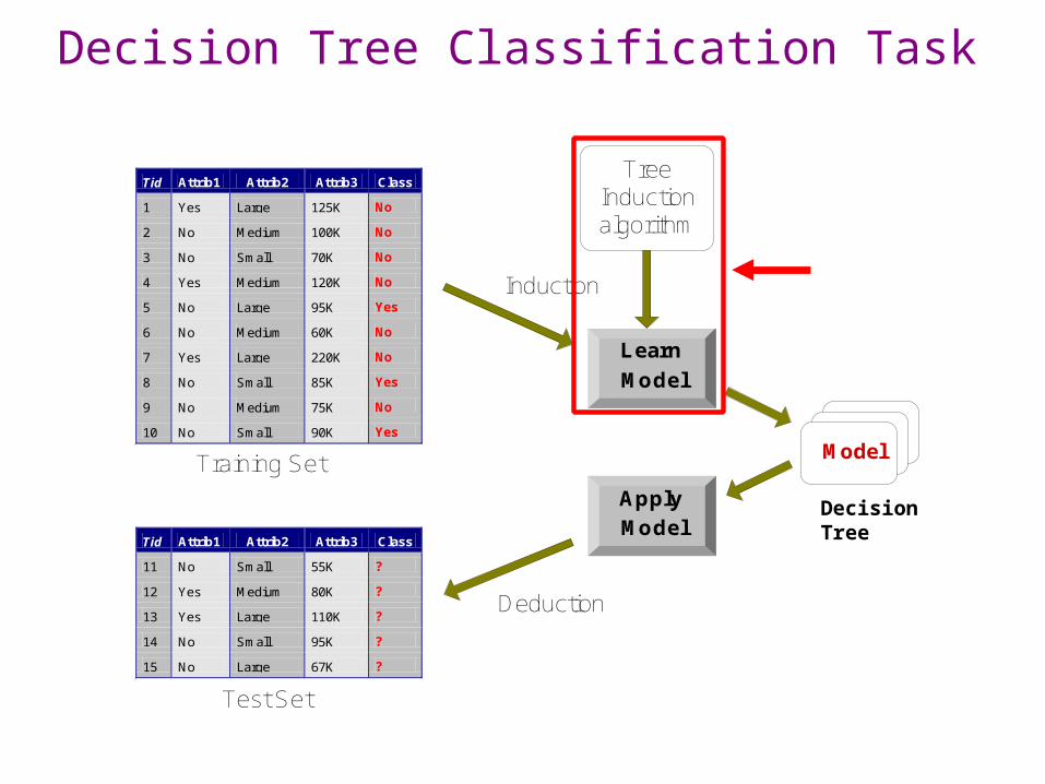
Illustrating Classification Task
Apply
Model
Induction
Deduction
Learn
Model
Model
Tid Attrib1 Attrib2 Attrib3 Class
1 Yes Large 125K No
2 No Medium 100K No
3 No Small 70K No
4 Yes Medium 120K No
5 No Large 95K Yes
6 No Medium 60K No
7 Yes Large 220K No
8 No Small 85K Yes
9 No Medium 75K No
10 No Small 90K Yes 10
Tid Attrib1 Attrib2 Attrib3 Class
11 No Small 55K ?
12 Yes Medium 80K ?
13 Yes Large 110K ?
14 No Small 95K ?
15 No Large 67K ? 10
Test Set
Learningalgorithm
Training Set

Examples of Classification Task
Predicting tumor cells as benign or malignant
Classifying credit card transactions as legitimate or fraudulent
Classifying secondary structures of protein as alpha-helix, beta-sheet, or random coil
Categorizing news stories as finance, weather, entertainment, sports, etc

Classification Techniques
Decision Tree based Methods Rule-based Methods Neural Networks Naïve Bayes and Bayesian Belief Networks Support Vector Machines

Example of a Decision Tree
Tid Refund MaritalStatus
TaxableIncome Cheat
1 Yes Single 125K No
2 No Married 100K No
3 No Single 70K No
4 Yes Married 120K No
5 No Divorced 95K Yes
6 No Married 60K No
7 Yes Divorced 220K No
8 No Single 85K Yes
9 No Married 75K No
10 No Single 90K Yes10
cate
goric
al
cate
goric
al
contin
uous
clas
s
Refund
MarSt
TaxInc
YESNO
NO
NO
Yes No
Married Single, Divorced
< 80K > 80K
Splitting Attributes
Training Data Model: Decision Tree

Another Example of Decision Tree
Tid Refund MaritalStatus
TaxableIncome Cheat
1 Yes Single 125K No
2 No Married 100K No
3 No Single 70K No
4 Yes Married 120K No
5 No Divorced 95K Yes
6 No Married 60K No
7 Yes Divorced 220K No
8 No Single 85K Yes
9 No Married 75K No
10 No Single 90K Yes10
cate
goric
al
cate
goric
al
contin
uous
clas
sMarSt
Refund
TaxInc
YESNO
NO
NO
Yes No
Married Single,
Divorced
< 80K > 80K
There could be more than one tree that fits the same data!

Decision Tree Classification Task
Apply
Model
Induction
Deduction
Learn
Model
Model
Tid Attrib1 Attrib2 Attrib3 Class
1 Yes Large 125K No
2 No Medium 100K No
3 No Small 70K No
4 Yes Medium 120K No
5 No Large 95K Yes
6 No Medium 60K No
7 Yes Large 220K No
8 No Small 85K Yes
9 No Medium 75K No
10 No Small 90K Yes 10
Tid Attrib1 Attrib2 Attrib3 Class
11 No Small 55K ?
12 Yes Medium 80K ?
13 Yes Large 110K ?
14 No Small 95K ?
15 No Large 67K ? 10
Test Set
TreeInductionalgorithm
Training Set
Decision Tree

Apply Model to Test Data
Refund
MarSt
TaxInc
YESNO
NO
NO
Yes No
Married Single, Divorced
< 80K > 80K
Refund Marital Status
Taxable Income Cheat
No Married 80K ? 10
Test DataStart from the root of
tree.

Apply Model to Test Data
Refund
MarSt
TaxInc
YESNO
NO
NO
Yes No
Married Single, Divorced
< 80K > 80K
Refund Marital Status
Taxable Income Cheat
No Married 80K ? 10
Test Data

Apply Model to Test Data
Refund
MarSt
TaxInc
YESNO
NO
NO
Yes No
Married Single, Divorced
< 80K > 80K
Refund Marital Status
Taxable Income Cheat
No Married 80K ? 10
Test Data

Apply Model to Test Data
Refund
MarSt
TaxInc
YESNO
NO
NO
Yes No
Married Single, Divorced
< 80K > 80K
Refund Marital Status
Taxable Income Cheat
No Married 80K ? 10
Test Data

Apply Model to Test Data
Refund
MarSt
TaxInc
YESNO
NO
NO
Yes No
Married Single, Divorced
< 80K > 80K
Refund Marital Status
Taxable Income Cheat
No Married 80K ? 10
Test Data

Apply Model to Test Data
Refund
MarSt
TaxInc
YESNO
NO
NO
Yes No
Married Single, Divorced
< 80K > 80K
Refund Marital Status
Taxable Income Cheat
No Married 80K ? 10
Test Data
Assign Cheat to “No”
Decision Tree Classification Task
Apply
Model
Induction
Deduction
Learn
Model
Model
Tid Attrib1 Attrib2 Attrib3 Class
1 Yes Large 125K No
2 No Medium 100K No
3 No Small 70K No
4 Yes Medium 120K No
5 No Large 95K Yes
6 No Medium 60K No
7 Yes Large 220K No
8 No Small 85K Yes
9 No Medium 75K No
10 No Small 90K Yes 10
Tid Attrib1 Attrib2 Attrib3 Class
11 No Small 55K ?
12 Yes Medium 80K ?
13 Yes Large 110K ?
14 No Small 95K ?
15 No Large 67K ? 10
Test Set
TreeInductionalgorithm
Training Set
Decision Tree
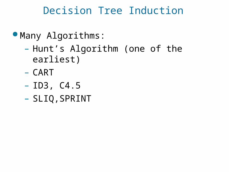
Decision Tree Induction
Many Algorithms:– Hunt’s Algorithm (one of the earliest)– CART– ID3, C4.5– SLIQ,SPRINT
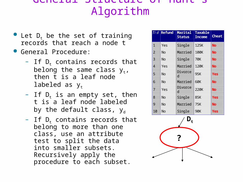
General Structure of Hunt’s Algorithm
Let Dt be the set of training records that reach a node t
General Procedure:– If Dt contains records that
belong the same class yt, then t is a leaf node labeled as yt
– If Dt is an empty set, then t is a leaf node labeled by the default class, yd
– If Dt contains records that belong to more than one class, use an attribute test to split the data into smaller subsets. Recursively apply the procedure to each subset.
Tid Refund Marital Status
Taxable Income Cheat
1 Yes Single 125K No
2 No Married 100K No
3 No Single 70K No
4 Yes Married 120K No
5 No Divorced
95K Yes
6 No Married 60K No
7 Yes Divorced
220K No
8 No Single 85K Yes
9 No Married 75K No
10 No Single 90K Yes 10
Dt
?
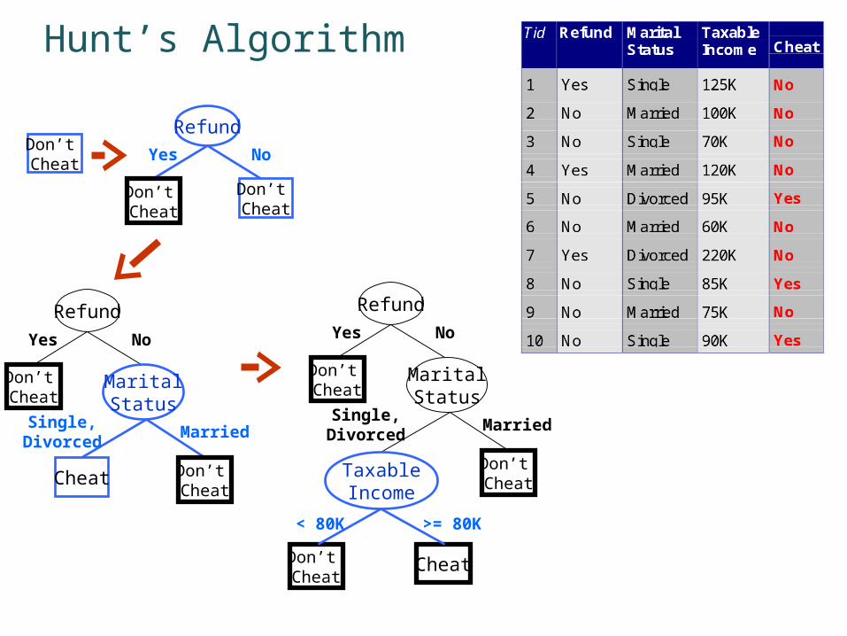
Hunt’s Algorithm
Don’t Cheat
Refund
Don’t Cheat
Don’t Cheat
Yes No
Refund
Don’t Cheat
Yes No
MaritalStatus
Don’t Cheat
Cheat
Single,Divorced
Married
TaxableIncome
Don’t Cheat
< 80K >= 80K
Refund
Don’t Cheat
Yes No
MaritalStatus
Don’t Cheat
Cheat
Single,Divorced
Married

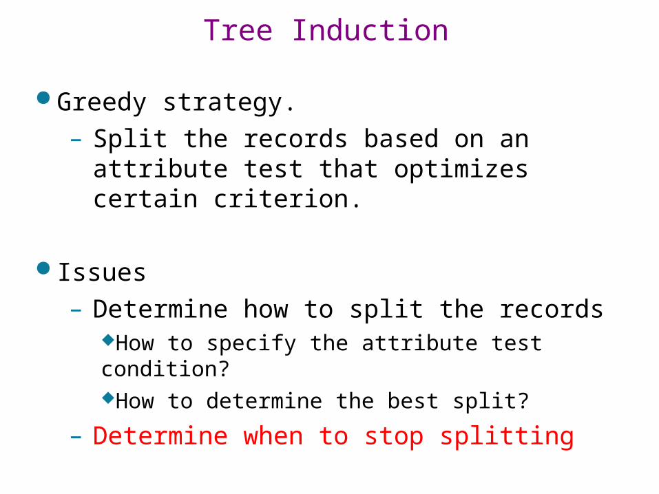
Tree Induction
Greedy strategy.– Split the records based on an attribute
test that optimizes certain criterion.
Issues– Determine how to split the records
How to specify the attribute test condition? How to determine the best split?
– Determine when to stop splitting

Tree Induction
Greedy strategy.– Split the records based on an attribute
test that optimizes certain criterion.
Issues– Determine how to split the records
How to specify the attribute test condition?How to determine the best split?
– Determine when to stop splitting

How to Specify Test Condition?
Depends on attribute types– Nominal– Ordinal– Continuous
Depends on number of ways to split– 2-way split– Multi-way split

Splitting Based on Nominal Attributes
Multi-way split: Use as many partitions as distinct values.
Binary split: Divides values into two subsets. Need to find optimal partitioning.
CarTypeFamily
Sports
Luxury
CarType{Family, Luxury} {Sports}
CarType{Sports,
Luxury}
{Family} OR
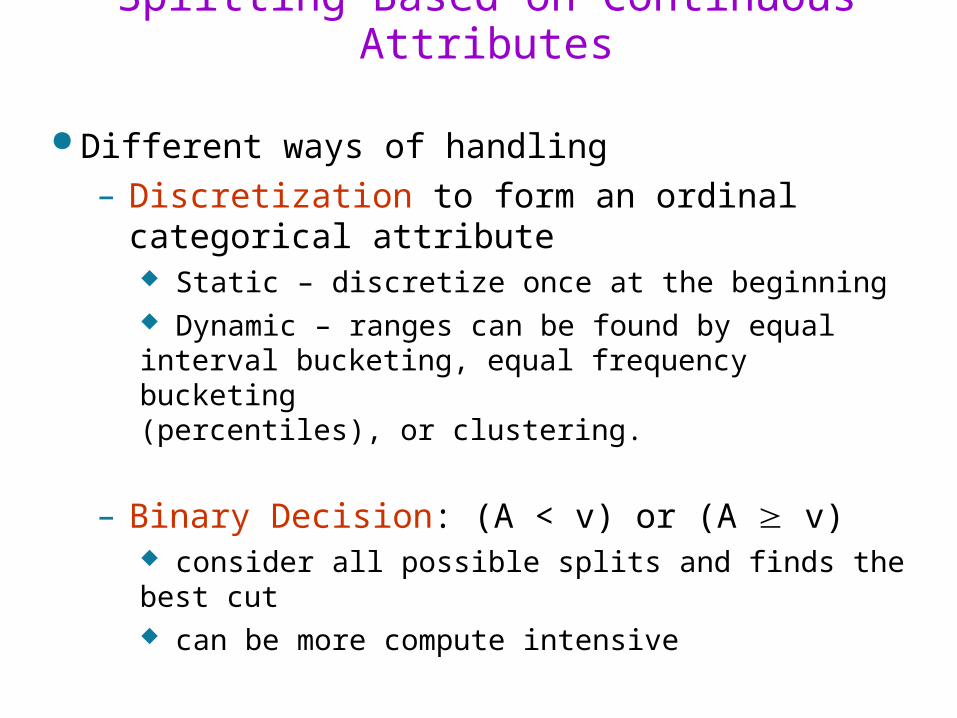
Splitting Based on Continuous Attributes
Different ways of handling– Discretization to form an ordinal
categorical attribute Static – discretize once at the beginning Dynamic – ranges can be found by equal interval bucketing, equal frequency bucketing(percentiles), or clustering.
– Binary Decision: (A < v) or (A v) consider all possible splits and finds the best cut can be more compute intensive

Splitting Based on Continuous Attributes
TaxableIncome> 80K?
Yes No
TaxableIncome?
(i) Binary split (ii) Multi-way split
< 10K
[10K,25K) [25K,50K) [50K,80K)
> 80K

Tree Induction
Greedy strategy.– Split the records based on an attribute
test that optimizes certain criterion.
Issues– Determine how to split the records
How to specify the attribute test condition?How to determine the best split?
– Determine when to stop splitting

How to determine the Best Split
OwnCar?
C0: 6C1: 4
C0: 4C1: 6
C0: 1C1: 3
C0: 8C1: 0
C0: 1C1: 7
CarType?
C0: 1C1: 0
C0: 1C1: 0
C0: 0C1: 1
StudentID?
...
Yes No Family
Sports
Luxury c1c10
c20
C0: 0C1: 1
...
c11
Before Splitting: 10 records of class 0, 10 records of class 1
Which test condition is the best?

How to determine the Best Split
Greedy approach: – Nodes with homogeneous class
distribution are preferred Need a measure of node impurity:
C0: 5C1: 5
C0: 9C1: 1
Non-homogeneous,
High degree of impurity
Homogeneous,
Low degree of impurity

Measures of Node Impurity
Gini Index
Entropy
Misclassification error

How to Find the Best Split
B?
Yes No
Node N3 Node N4
A?
Yes No
Node N1 Node N2
Before Splitting:
C0 N10 C1 N11
C0 N20 C1 N21
C0 N30 C1 N31
C0 N40 C1 N41
C0 N00 C1 N01
M0
M1 M2 M3 M4
M12 M34
Gain = M0 – M12 vs M0 – M34

Measure of Impurity: GINI
Gini Index for a given node t :
(NOTE: p( j | t) is the relative frequency of class j at node t).
– Maximum (1 - 1/nc) when records are equally distributed among all classes, implying least interesting information
– Minimum (0.0) when all records belong to one class, implying most interesting information
j
tjptGINI 2)]|([1)(
C1 0C2 6
Gini=0.000
C1 2C2 4
Gini=0.444
C1 3C2 3
Gini=0.500
C1 1C2 5
Gini=0.278

Examples for computing GINI
C1 0
C2 6
C1 2
C2 4
C1 1
C2 5
P(C1) = 0/6 = 0 P(C2) = 6/6 = 1
Gini = 1 – P(C1)2 – P(C2)2 = 1 – 0 – 1 = 0
j
tjptGINI 2)]|([1)(
P(C1) = 1/6 P(C2) = 5/6
Gini = 1 – (1/6)2 – (5/6)2 = 0.278
P(C1) = 2/6 P(C2) = 4/6
Gini = 1 – (2/6)2 – (4/6)2 = 0.444

Splitting Based on GINI
Used in CART, SLIQ, SPRINT. When a node p is split into k partitions (children),
the quality of split is computed as,
where, ni = number of records at child i,
n = number of records at node p.
k
i
isplit iGINI
n
nGINI
1
)(

Binary Attributes: Computing GINI Index
Splits into two partitions Effect of Weighing partitions:
– Larger and Purer Partitions are sought for.
B?
Yes No
Node N1 Node N2
Parent
C1 6
C2 6
Gini = 0.500
N1 N2 C1 5 1
C2 2 4
Gini=0.333
Gini(N1) = 1 – (5/6)2 – (2/6)2 = 0.194
Gini(N2) = 1 – (1/6)2 – (4/6)2 = 0.528
Gini(Children) = 7/12 * 0.194 + 5/12 * 0.528= 0.333

Categorical Attributes: Computing Gini Index
For each distinct value, gather counts for each class in the dataset
Use the count matrix to make decisions
CarType {Sports,
Luxury} {Family}
C1 3 1
C2 2 4
Gini 0.400
CarType {Sports} {Family,Luxury}
C1 2 2
C2 1 5
Gini 0.419
CarType Family Sports Luxury
C1 1 2 1 C2 4 1 1 Gini 0.393
Multi-way split Two-way split (find best partition of values)

Continuous Attributes: Computing Gini Index Use Binary Decisions based on one value
Several Choices for the splitting value
– Number of possible splitting values = Number of distinct values
Each splitting value has a count matrix associated with it
– Class counts in each of the partitions, A < v and A v
Simple method to choose best v– For each v, scan the
database to gather count matrix and compute its Gini index
– Computationally Inefficient! Repetition of work.
TaxableIncome> 80K?
Yes No

Continuous Attributes: Computing Gini Index...
For efficient computation: for each attribute,– Sort the attribute on values– Linearly scan these values, each time updating the count matrix and computing gini index
– Choose the split position that has the least gini index
Cheat No No No Yes Yes Yes No No No No
Taxable Income
60 70 75 85 90 95 100 120 125 220
55 65 72 80 87 92 97 110 122 172 230
<= > <= > <= > <= > <= > <= > <= > <= > <= > <= > <= >
Yes 0 3 0 3 0 3 0 3 1 2 2 1 3 0 3 0 3 0 3 0 3 0
No 0 7 1 6 2 5 3 4 3 4 3 4 3 4 4 3 5 2 6 1 7 0
Gini 0.420 0.400 0.375 0.343 0.417 0.400 0.300 0.343 0.375 0.400 0.420
Split Positions
Sorted Values

Alternative Splitting Criteria based on INFO
Entropy at a given node t:
(NOTE: p( j | t) is the relative frequency of class j at node t).
– Measures homogeneity of a node. Maximum (log nc) when records are equally
distributed among all classes implying least information
Minimum (0.0) when all records belong to one class, implying most information
– Entropy based computations are similar to the GINI index computations
j
tjptjptEntropy )|(log)|()(

Examples for computing Entropy
C1 0
C2 6
C1 2
C2 4
C1 1
C2 5
P(C1) = 0/6 = 0 P(C2) = 6/6 = 1
Entropy = – 0 log 0 – 1 log 1 = – 0 – 0 = 0
P(C1) = 1/6 P(C2) = 5/6
Entropy = – (1/6) log2 (1/6) – (5/6) log2 (1/6) = 0.65
P(C1) = 2/6 P(C2) = 4/6
Entropy = – (2/6) log2 (2/6) – (4/6) log2 (4/6) = 0.92
j
tjptjptEntropy )|(log)|()(2

Splitting Based on INFO...
Information Gain:
Parent Node, p is split into k partitions;
ni is number of records in partition i
– Measures Reduction in Entropy achieved because of the split. Choose the split that achieves most reduction (maximizes GAIN)
– Used in ID3 and C4.5– Disadvantage: Tends to prefer splits that result in
large number of partitions, each being small but pure.
k
i
i
splitiEntropy
nn
pEntropyGAIN1
)()(

Splitting Based on INFO...
Gain Ratio:
Parent Node, p is split into k partitions
ni is the number of records in partition i
– Adjusts Information Gain by the entropy of the partitioning (SplitINFO). Higher entropy partitioning (large number of small partitions) is penalized!
– Used in C4.5– Designed to overcome the disadvantage of
Information Gain
SplitINFO
GAINGainRATIO Split
split
k
i
ii
nn
nn
SplitINFO1
log

Splitting Criteria based on Classification Error
Classification error at a node t :
Measures misclassification error made by a node. Maximum (1 - 1/nc) when records are equally
distributed among all classes, implying least interesting information
Minimum (0.0) when all records belong to one class, implying most interesting information
)|(max1)( tiPtErrori

Examples for Computing Error
C1 0 C2 6
C1 2 C2 4
C1 1 C2 5
P(C1) = 0/6 = 0 P(C2) = 6/6 = 1
Error = 1 – max (0, 1) = 1 – 1 = 0
P(C1) = 1/6 P(C2) = 5/6
Error = 1 – max (1/6, 5/6) = 1 – 5/6 = 1/6
P(C1) = 2/6 P(C2) = 4/6
Error = 1 – max (2/6, 4/6) = 1 – 4/6 = 1/3
)|(max1)( tiPtErrori

Misclassification Error vs Gini
A?
Yes No
Node N1 Node N2
Parent
C1 7
C2 3
Gini = 0.42
N1 N2 C1 3 4
C2 0 3
Gini=0.361
Gini(N1) = 1 – (3/3)2 – (0/3)2 = 0
Gini(N2) = 1 – (4/7)2 – (3/7)2 = 0.489
Gini(Children) = 3/10 * 0 + 7/10 * 0.489= 0.342
Gini improves !!
Tree Induction
Greedy strategy.– Split the records based on an attribute
test that optimizes certain criterion.
Issues– Determine how to split the records
How to specify the attribute test condition?How to determine the best split?
– Determine when to stop splitting

Stopping Criteria for Tree Induction
Stop expanding a node when all the records belong to the same class
Stop expanding a node when all the records have similar attribute values
Early termination (to be discussed later)

Decision Tree Based Classification
Advantages:– Inexpensive to construct– Extremely fast at classifying unknown
records– Easy to interpret for small-sized trees– Accuracy is comparable to other
classification techniques for many simple data sets

Example: C4.5
Simple depth-first construction. Uses Information Gain Sorts Continuous Attributes at each node. Needs entire data to fit in memory. Unsuitable for Large Datasets.
– Needs out-of-core sorting.
You can download the software from:http://www.cse.unsw.edu.au/~quinlan/c4.5r8.tar.gz

Practical Issues of Classification
Underfitting and Overfitting
Missing Values
Costs of Classification

Underfitting and Overfitting (Example)
500 circular and 500 triangular data points.
Circular points:
0.5 sqrt(x12+x2
2) 1
Triangular points:
sqrt(x12+x2
2) > 0.5 or
sqrt(x12+x2
2) < 1

Underfitting and Overfitting
Overfitting
Underfitting: when model is too simple, both training and test errors are large

Overfitting due to Noise
Decision boundary is distorted by noise point

Overfitting due to Insufficient Examples
Lack of data points in the lower half of the diagram makes it difficult to predict correctly the class labels of that region
- Insufficient number of training records in the region causes the decision tree to predict the test examples using other training records that are irrelevant to the classification task

Notes on Overfitting
Overfitting results in decision trees that are more complex than necessary
Training error no longer provides a good estimate of how well the tree will perform on previously unseen records
Need new ways for estimating errors