Classification: Basic Concepts, Decision Trees, and Model...

Classification: Basic Concepts, Decision Trees, and Model Evaluation

Dr. Hui XiongRutgers University

Introduction to Data Mining 1/2/2009 1

Classification: Definition

Given a collection of records (training set )– Each record is by characterized by a tuple

( ) h i th tt ib t t d i th(x,y), where x is the attribute set and y is the class label

x: attribute, predictor, independent variable, inputy: class, response, dependent variable, output

Task:


Task:– Learn a model that maps each attribute set x

into one of the predefined class labels y

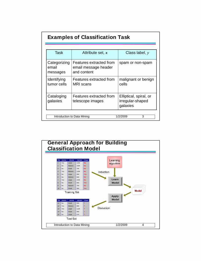
Examples of Classification Task

Task Attribute set, x Class label, y

C t i i F t t t d fCategorizing email messages

Features extracted from email message header and content

spam or non-spam

Identifying tumor cells

Features extracted from MRI scans

malignant or benign cells


Cataloging galaxies

Features extracted from telescope images

Elliptical, spiral, or irregular-shaped galaxies

General Approach for Building Classification Model

Tid Attrib1 Attrib2 Attrib3 Class

1 Yes Large 125K No

2 No Medium 100K No

3 No Small 70K No

Apply Model

Learn Model

4 Yes Medium 120K No

5 No Large 95K Yes

6 No Medium 60K No

7 Yes Large 220K No

8 No Small 85K Yes

9 No Medium 75K No

10 No Small 90K Yes 10


ModelTid Attrib1 Attrib2 Attrib3 Class

11 No Small 55K ?

12 Yes Medium 80K ?

13 Yes Large 110K ?

14 No Small 95K ?

15 No Large 67K ? 10

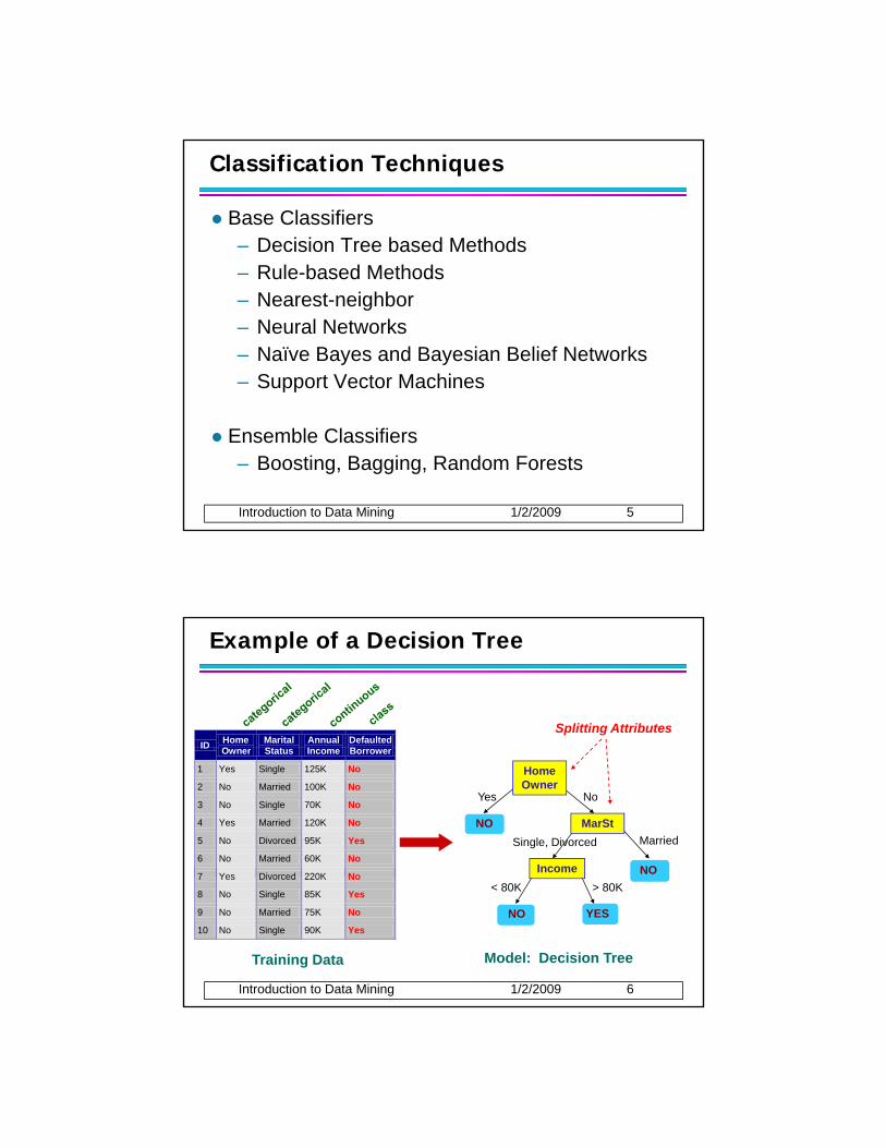
Classification Techniques

Base Classifiers– Decision Tree based Methods

Rule based Methods– Rule-based Methods– Nearest-neighbor– Neural Networks– Naïve Bayes and Bayesian Belief Networks– Support Vector Machines


Ensemble Classifiers– Boosting, Bagging, Random Forests

Example of a Decision Tree

ID Home Marital Annual Defaulted Splitting Attributes

ID Owner Status Income Borrower

1 Yes Single 125K No

2 No Married 100K No

3 No Single 70K No

4 Yes Married 120K No

5 No Divorced 95K Yes

6 No Married 60K No

7 Yes Divorced 220K No

Home Owner

MarSt

Income

NO

NO

Yes No

MarriedSingle, Divorced



8 No Single 85K Yes

9 No Married 75K No

10 No Single 90K Yes 10

YESNO

< 80K > 80K

Training Data Model: Decision Tree

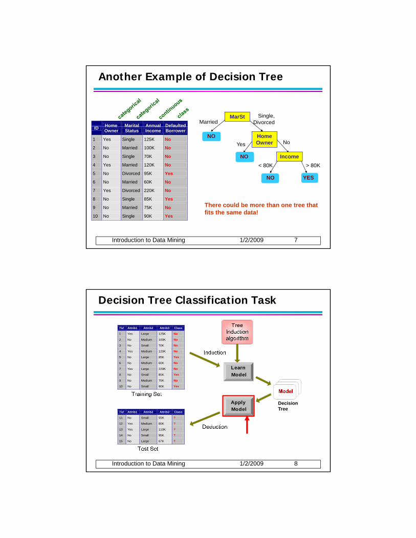
Another Example of Decision Tree

MarStMarried

Single, Divorced

ID Home Marital Annual Defaulted

Home Owner

Income

YESNO

NO

NO

Yes No

< 80K > 80K

ID Home Owner

Marital Status

Annual Income

Defaulted Borrower



3 No Single 70K No



6 No Married 60K No


There could be more than one tree that fits the same data!


8 No Single 85K Yes

9 No Married 75K No


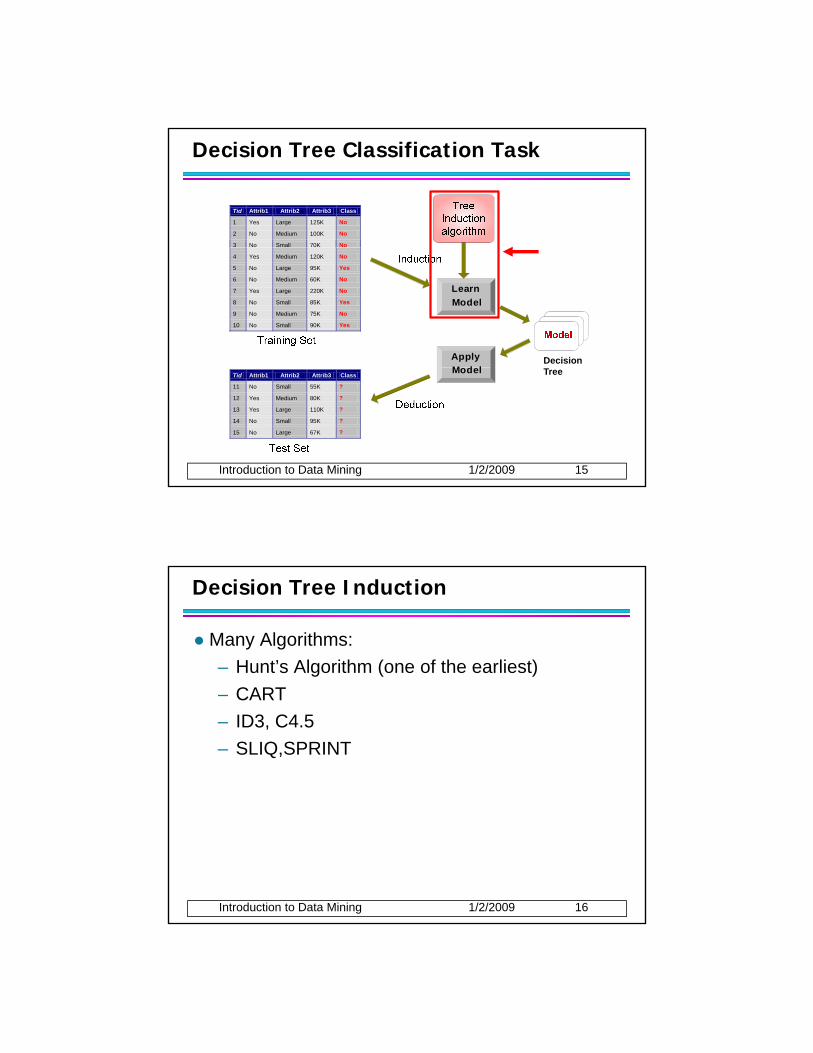
Decision Tree Classification Task


1 Yes Large 125K No

2 No Medium 100K No

3 No Small 70K No

Apply Model

Learn Model


5 No Large 95K Yes

6 No Medium 60K No

7 Yes Large 220K No

8 No Small 85K Yes

9 No Medium 75K No


Tid Att ib1 Att ib2 Att ib3 Cl

Decision Tree



11 No Small 55K ?

12 Yes Medium 80K ?

13 Yes Large 110K ?

14 No Small 95K ?


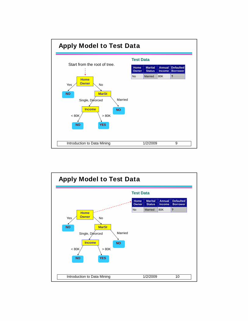
Apply Model to Test Data

Home Owner

Marital Status

Annual Income

Defaulted Borrower

N M i d 80K ?

Test DataStart from the root of tree.

Home Owner

MarSt

Income

NO

NO

Yes No


No Married 80K ?10


YESNO

< 80K > 80K


Home Owner

Marital Status

Annual Income

Defaulted Borrower

N M i d 80K ?

Test Data

MarSt

Income

NO

NO

Yes No


No Married 80K ?10

Home Owner


YESNO

< 80K > 80K


Home Owner

Marital Status

Annual Income

Defaulted Borrower

N M i d 80K ?

Test Data

MarSt

Income

NO

NO

Yes No


No Married 80K ?10

Home Owner


YESNO

< 80K > 80K


Home Owner

Marital Status

Annual Income

Defaulted Borrower

N M i d 80K ?

Test Data

MarSt

Income

NO

NO

Yes No


No Married 80K ?10

Home Owner


YESNO

< 80K > 80K


Home Owner

Marital Status

Annual Income

Defaulted Borrower

N M i d 80K ?

Test Data

MarSt

Income

NO

NO

Yes No

Married Single, Divorced

No Married 80K ?10

Home Owner


YESNO

< 80K > 80K


Home Owner

Marital Status

Annual Income

Defaulted Borrower

N M i d 80K ?

Test Data

MarSt

Income

NO

NO

Yes No

Married Single, Divorced

No Married 80K ?10

Assign Defaulted to “No”

Home Owner


YESNO

< 80K > 80K

Decision Tree Classification Task


1 Yes Large 125K No

2 No Medium 100K No

3 No Small 70K No

Apply M d l

Learn Model


5 No Large 95K Yes

6 No Medium 60K No

7 Yes Large 220K No

8 No Small 85K Yes

9 No Medium 75K No


Decision


ModelTid Attrib1 Attrib2 Attrib3 Class

11 No Small 55K ?

12 Yes Medium 80K ?

13 Yes Large 110K ?

14 No Small 95K ?


Tree

Decision Tree Induction

Many Algorithms:– Hunt’s Algorithm (one of the earliest)– CART– ID3, C4.5– SLIQ,SPRINT


General Structure of Hunt’s Algorithm

Let Dt be the set of training records that reach a node t

General Procedure:

ID Home Owner

Marital Status

Annual Income

Defaulted Borrower



3 No Single 70K No General Procedure:– If Dt contains records that

belong the same class yt, then t is a leaf node labeled as yt

– If Dt contains records that belong to more than one l tt ib t t t Dt

g o



6 No Married 60K No


8 No Single 85K Yes

9 No Married 75K No



class, use an attribute test to split the data into smaller subsets. Recursively apply the procedure to each subset.

t

?

Hunt’s Algorithm

ID Home Owner

Marital Status

Annual Income

Defaulted Borrower



3 No Single 70K No



6 No Married 60K No


8 No Single 85K Yes

9 No Married 75K No



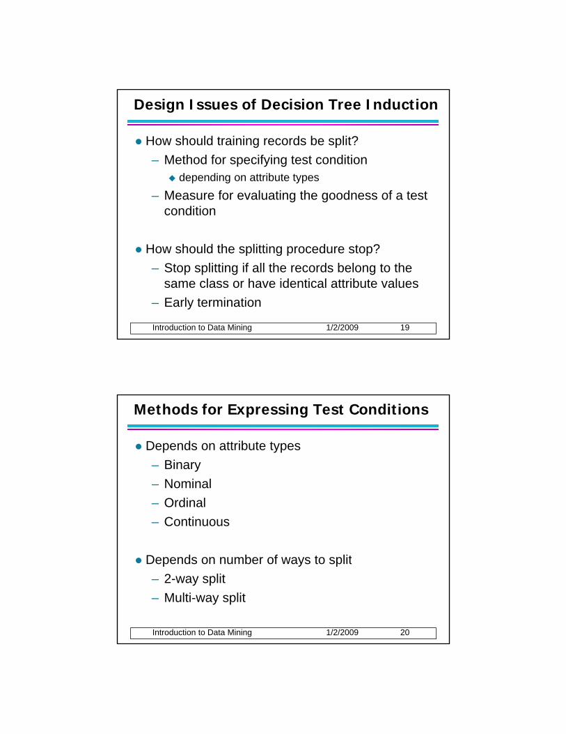
Design Issues of Decision Tree Induction

How should training records be split?– Method for specifying test condition

depending on attribute types

– Measure for evaluating the goodness of a test condition

How should the splitting procedure stop?


– Stop splitting if all the records belong to the same class or have identical attribute values

– Early termination

Methods for Expressing Test Conditions

Depends on attribute types– Binary– Nominal– Ordinal– Continuous

Depends on number of ways to split


Depends on number of ways to split– 2-way split– Multi-way split

Test Condition for Nominal Attributes

Multi-way split:– Use as many partitions as

distinct values.distinct values.

Binary split:– Divides values into two subsets– Need to find optimal


eed o d op apartitioning.

Test Condition for Ordinal Attributes

Multi-way split:– Use as many partitions

as distinct valuesas distinct values

Binary split:– Divides values into two

subsets– Need to find optimal


partitioning– Preserve the order

property among attribute values

This grouping violates order property

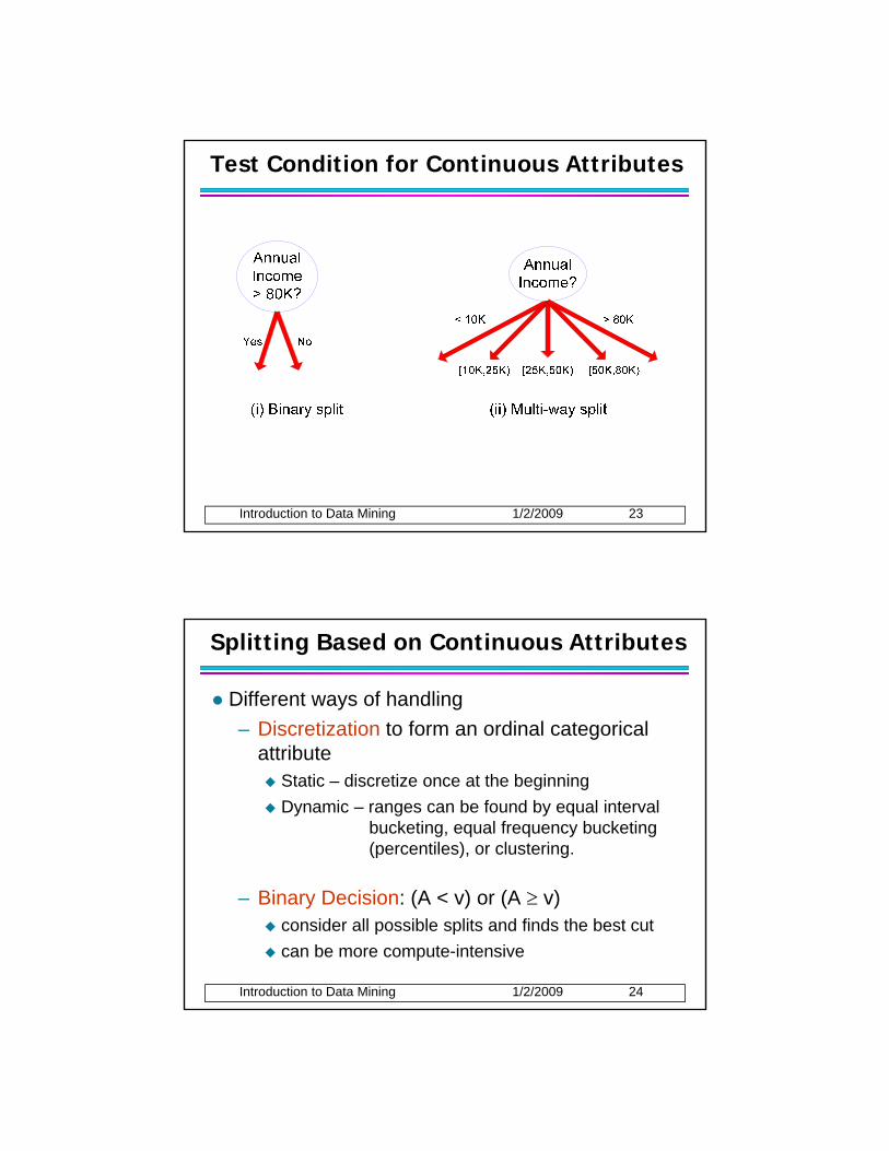
Test Condition for Continuous Attributes


Splitting Based on Continuous Attributes

Different ways of handling– Discretization to form an ordinal categorical

tt ib tattributeStatic – discretize once at the beginningDynamic – ranges can be found by equal interval

bucketing, equal frequency bucketing(percentiles), or clustering.


– Binary Decision: (A < v) or (A ≥ v)consider all possible splits and finds the best cutcan be more compute-intensive

How to determine the Best Split

Before Splitting: 10 records of class 0,10 records of class 1

Introduction to Data Mining 1/2/2009 25Which test condition is the best?

How to determine the Best Split

Greedy approach: – Nodes with purer class distribution are

f dpreferred

Need a measure of node impurity:


High degree of impurity Low degree of impurity

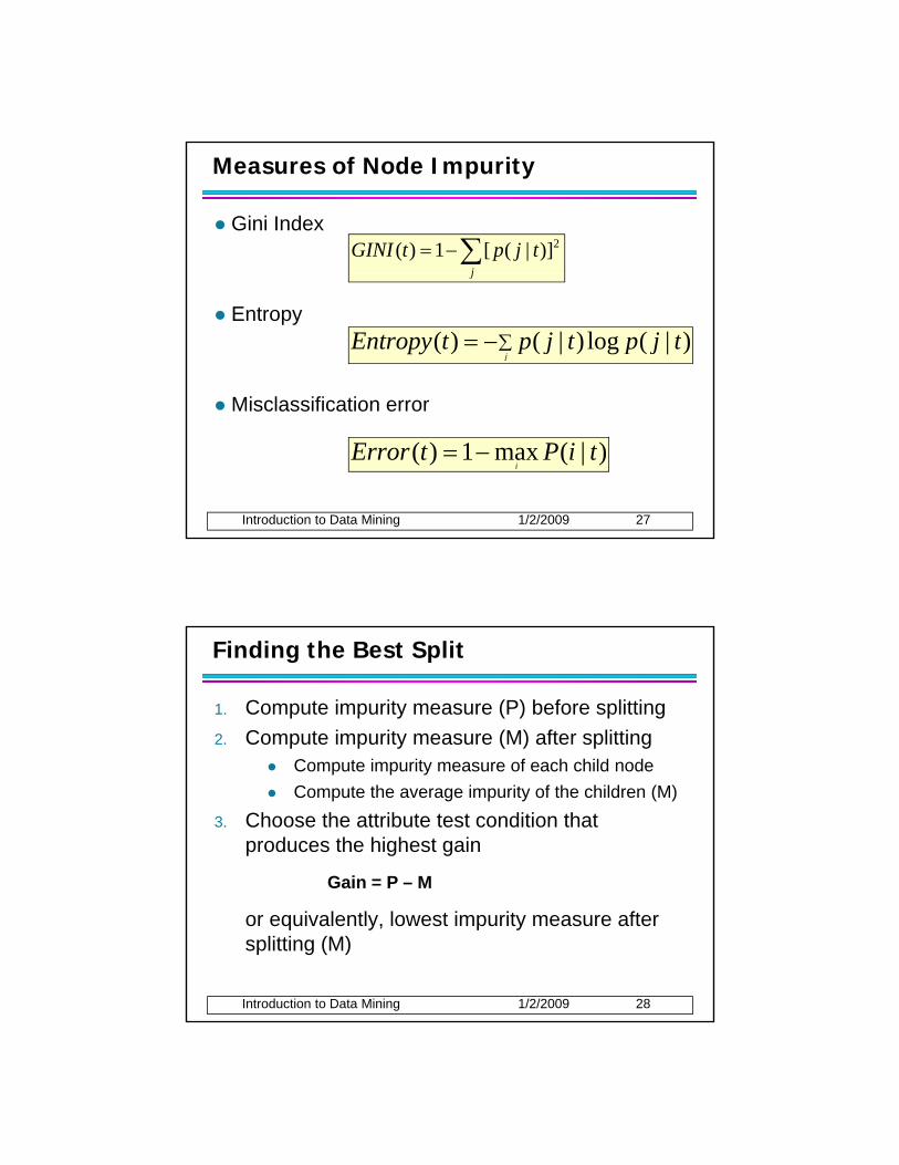
Measures of Node Impurity

Gini Index∑−=

j

tjptGINI 2)]|([1)(

Entropy

Misclassification error

j

∑−=j

tjptjptEntropy )|(log)|()(


Misclassification error

)|(max1)( tiPtErrori

−=

Finding the Best Split

1. Compute impurity measure (P) before splitting2. Compute impurity measure (M) after splitting

Compute impurity measure of each child nodeCompute the average impurity of the children (M)

3. Choose the attribute test condition that produces the highest gain

Gain = P – M


or equivalently, lowest impurity measure after splitting (M)

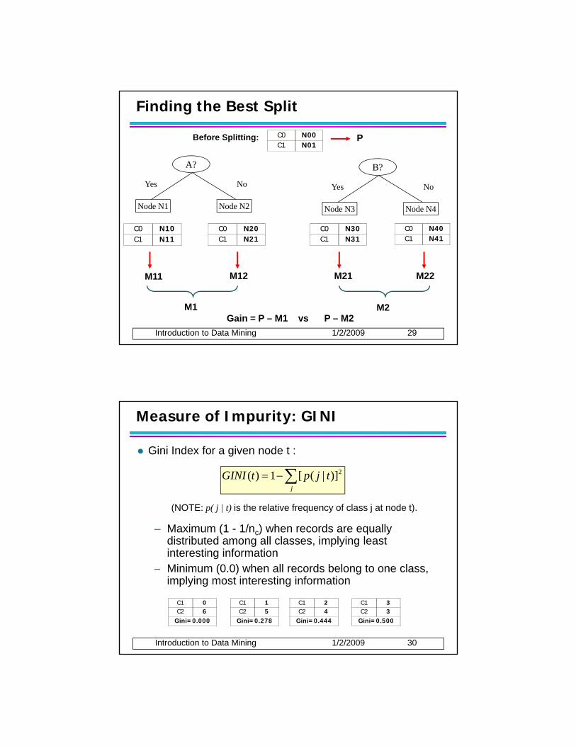
Finding the Best Split

B?A?

Before Splitting: C0 N00 C1 N01

P

Yes No

Node N3 Node N4

Yes No

Node N1 Node N2

C0 N10 C1 N11

C0 N20 C1 N21

C0 N30 C1 N31

C0 N40 C1 N41


M11 M12 M21 M22

M1 M2Gain = P – M1 vs P – M2

Measure of Impurity: GINI

Gini Index for a given node t :

∑−= tjptGINI 2)]|([1)(

(NOTE: p( j | t) is the relative frequency of class j at node t).

– Maximum (1 - 1/nc) when records are equally distributed among all classes, implying least interesting information

– Minimum (0 0) when all records belong to one class

j


Minimum (0.0) when all records belong to one class, implying most interesting information

C1 0C2 6

Gini=0.000

C1 2C2 4

Gini=0.444

C1 3C2 3

Gini=0.500

C1 1C2 5

Gini=0.278

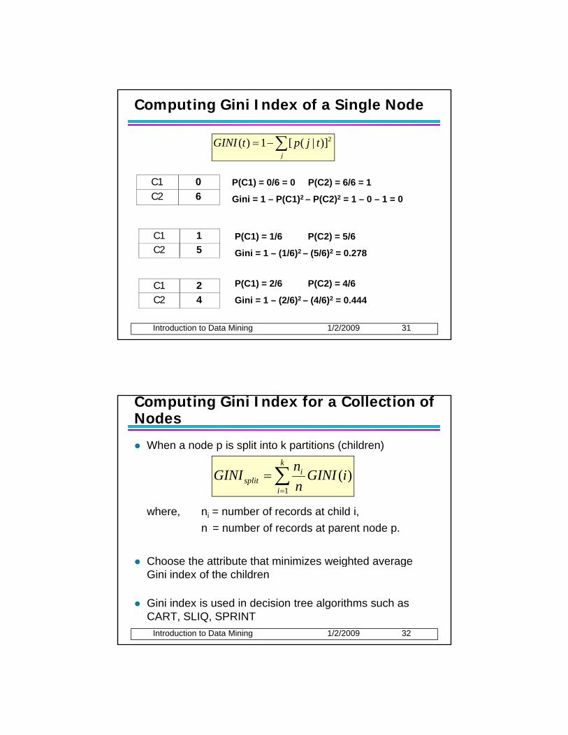
Computing Gini Index of a Single Node

∑−=j

tjptGINI 2)]|([1)(

C1 0 C2 6

C1 1 C2 5

P(C1) = 0/6 = 0 P(C2) = 6/6 = 1

Gini = 1 – P(C1)2 – P(C2)2 = 1 – 0 – 1 = 0

P(C1) = 1/6 P(C2) = 5/6

Gini = 1 – (1/6)2 – (5/6)2 = 0.278


C1 2 C2 4

( ) ( )

P(C1) = 2/6 P(C2) = 4/6

Gini = 1 – (2/6)2 – (4/6)2 = 0.444

Computing Gini Index for a Collection of Nodes

When a node p is split into k partitions (children)

∑=k

ili iGINInGINI )(

where, ni = number of records at child i,n = number of records at parent node p.

Choose the attribute that minimizes weighted average

∑=i

split iGINIn

GINI1

)(


Choose the attribute that minimizes weighted average Gini index of the children

Gini index is used in decision tree algorithms such as CART, SLIQ, SPRINT

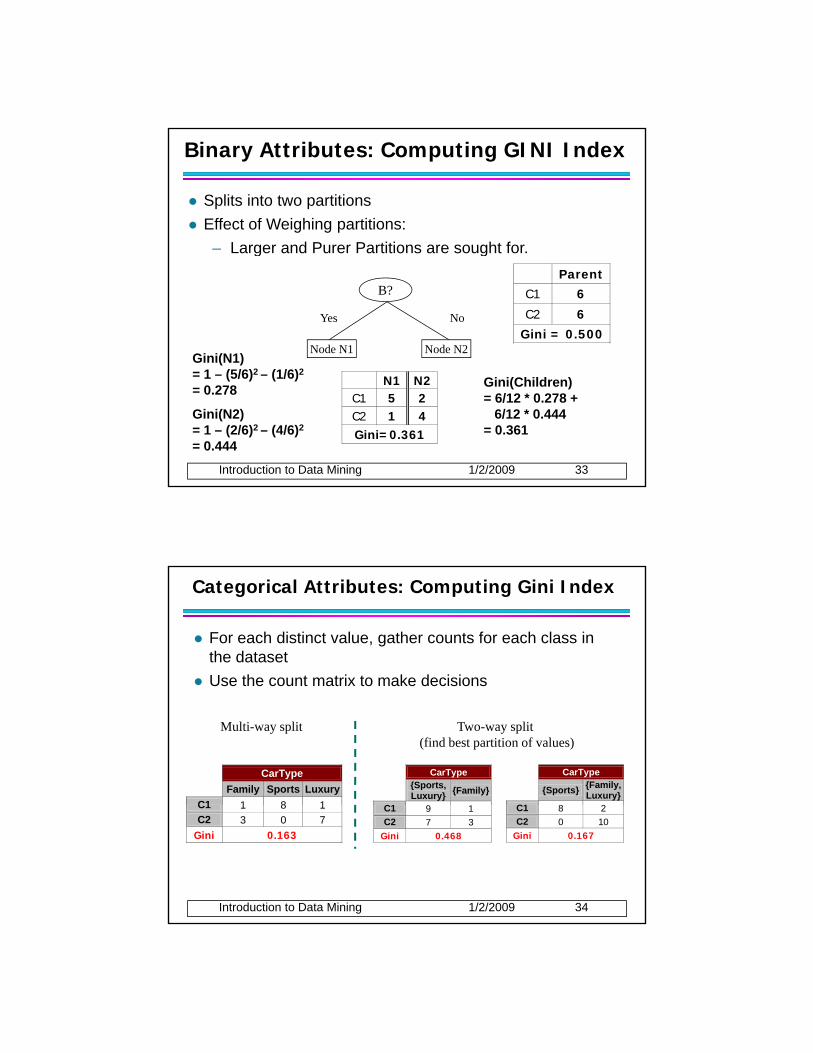
Binary Attributes: Computing GINI Index

Splits into two partitionsEffect of Weighing partitions:

Larger and Purer Partitions are sought for– Larger and Purer Partitions are sought for.

B?

Yes No

Node N1 Node N2

Parent C1 6

C2 6

Gini = 0.500

Gini(N1)


N1 N2C1 5 2 C2 1 4 Gini=0.361

= 1 – (5/6)2 – (1/6)2

= 0.278

Gini(N2) = 1 – (2/6)2 – (4/6)2

= 0.444

Gini(Children) = 6/12 * 0.278 +

6/12 * 0.444= 0.361

Categorical Attributes: Computing Gini Index

For each distinct value, gather counts for each class in the datasetUse the count matrix to make decisionsUse the count matrix to make decisions

CarType {Sports,

Luxury} {Family}

C1

CarType {Sports} {Family,

Luxury} C1 8 2

CarType Family Sports Luxury

C1 1 8 1

Multi-way split Two-way split (find best partition of values)


C1 9 1C2 7 3

Gini 0.468

C1 8 2 C2 0 10

Gini 0.167

C1 1 8 1 C2 3 0 7

Gini 0.163

Continuous Attributes: Computing Gini Index

Use Binary Decisions based on one valueSeveral Choices for the splitting value

Number of possible splitting values

ID Home Owner

Marital Status

Annual Income Defaulted



3 N Si l 70K N– Number of possible splitting values = Number of distinct values

Each splitting value has a count matrix associated with it

– Class counts in each of the partitions, A < v and A ≥ v

Simple method to choose best v– For each v scan the database to

3 No Single 70K No



6 No Married 60K No


8 No Single 85K Yes

9 No Married 75K No



– For each v, scan the database to gather count matrix and compute its Gini index

– Computationally Inefficient! Repetition of work.

Continuous Attributes: Computing Gini Index...

For efficient computation: for each attribute,– Sort the attribute on values– Linearly scan these values, each time updating the count matrix

d i i i i dand computing gini index– Choose the split position that has the least gini index

Cheat No No No Yes Yes Yes No No No No

Annual Income

60 70 75 85 90 95 100 120 125 220

55 65 72 80 87 92 97 110 122 172 230 Split PositionsSorted Values


<= > <= > <= > <= > <= > <= > <= > <= > <= > <= > <= >

Yes 0 3 0 3 0 3 0 3 1 2 2 1 3 0 3 0 3 0 3 0 3 0

No 0 7 1 6 2 5 3 4 3 4 3 4 3 4 4 3 5 2 6 1 7 0

Gini 0.420 0.400 0.375 0.343 0.417 0.400 0.300 0.343 0.375 0.400 0.420

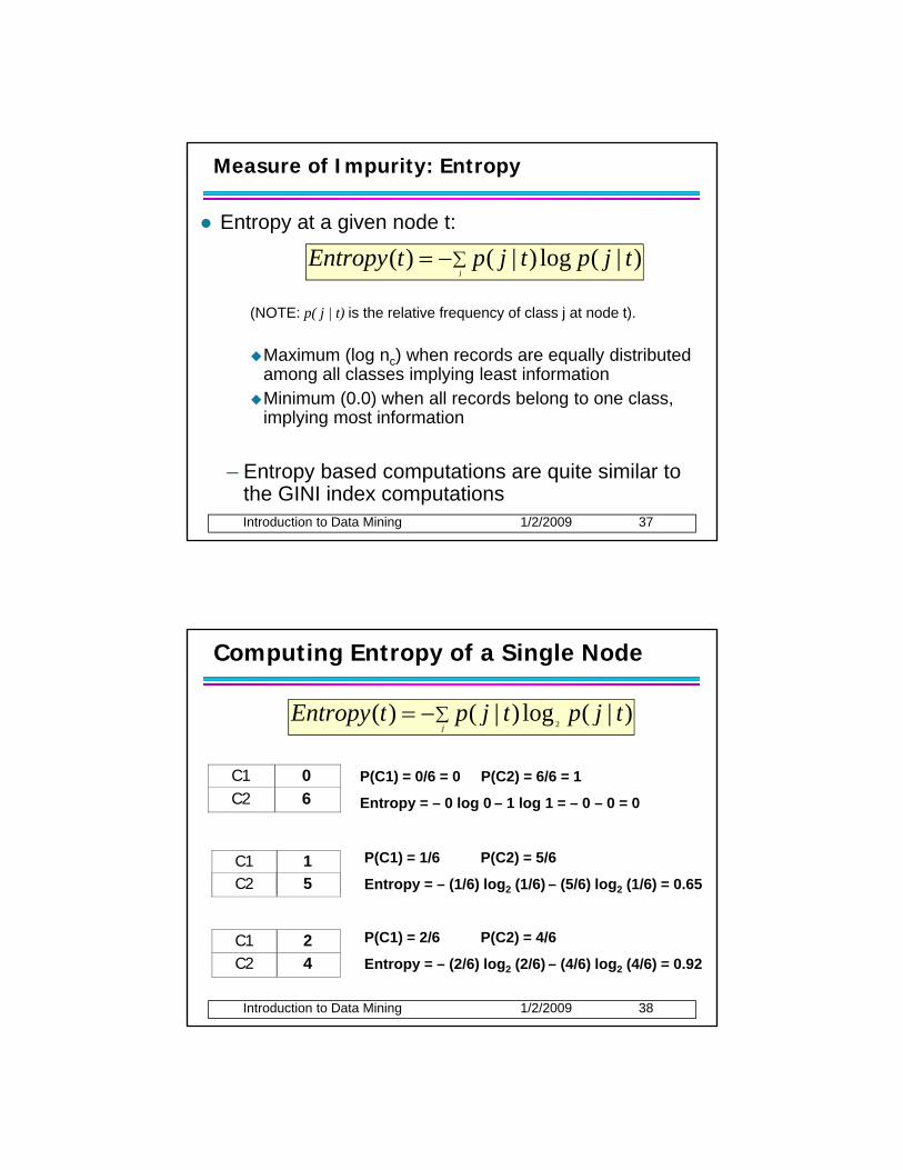
Measure of Impurity: Entropy

Entropy at a given node t:

∑−=j

tjptjptEntropy )|(log)|()(

(NOTE: p( j | t) is the relative frequency of class j at node t).

Maximum (log nc) when records are equally distributed among all classes implying least informationMinimum (0.0) when all records belong to one class,

j


implying most information

– Entropy based computations are quite similar to the GINI index computations

Computing Entropy of a Single Node

∑−=j

tjptjptEntropy )|(log)|()(2

C1 0 C2 6

C1 1 C2 5

P(C1) = 0/6 = 0 P(C2) = 6/6 = 1

Entropy = – 0 log 0 – 1 log 1 = – 0 – 0 = 0

P(C1) = 1/6 P(C2) = 5/6

Entropy = – (1/6) log2 (1/6) – (5/6) log2 (1/6) = 0.65


C1 2 C2 4

P(C1) = 2/6 P(C2) = 4/6

Entropy = – (2/6) log2 (2/6) – (4/6) log2 (4/6) = 0.92

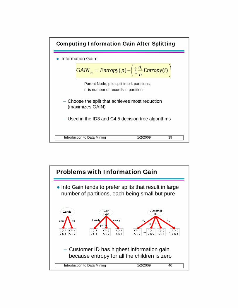
Computing Information Gain After Splitting

Information Gain:

⎟⎠⎞

⎜⎝⎛−= ∑

ki

litiEntropynpEntropyGAIN )()(

Parent Node, p is split into k partitions;ni is number of records in partition i

– Choose the split that achieves most reduction (maximizes GAIN)

⎟⎠

⎜⎝ =isplit

pyn

ppy1

)()(


(maximizes GAIN)

– Used in the ID3 and C4.5 decision tree algorithms

Problems with Information Gain

Info Gain tends to prefer splits that result in large number of partitions, each being small but pure


– Customer ID has highest information gain because entropy for all the children is zero

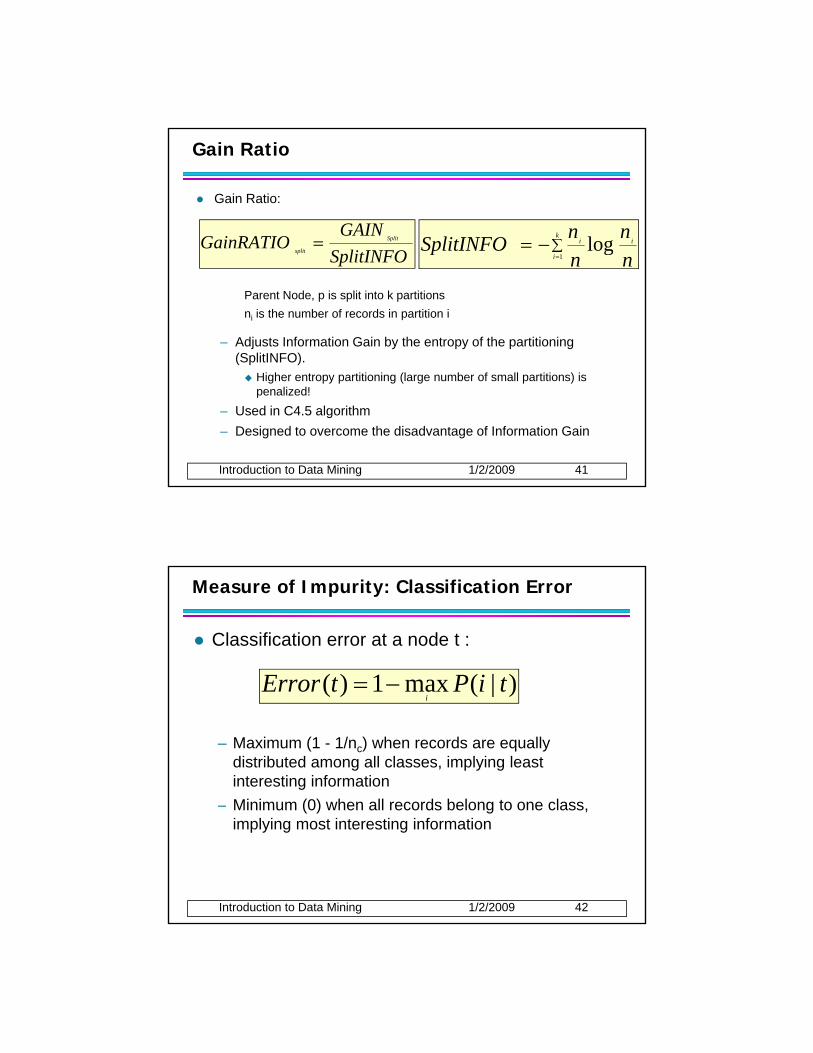
Gain Ratio

Gain Ratio:

GAINGainRATIO Split= ∑−=

kii

nnSplitINFO log

Parent Node, p is split into k partitionsni is the number of records in partition i

– Adjusts Information Gain by the entropy of the partitioning (SplitINFO).

SplitINFOGainRATIO

split ∑=

=i nn

SplitINFO1

log


Higher entropy partitioning (large number of small partitions) is penalized!

– Used in C4.5 algorithm– Designed to overcome the disadvantage of Information Gain

Measure of Impurity: Classification Error

Classification error at a node t :

)|(max1)( tiPtError −=

– Maximum (1 - 1/nc) when records are equally distributed among all classes, implying least interesting informationMinimum (0) when all records belong to one class


−=


– Minimum (0) when all records belong to one class, implying most interesting information

Computing Error of a Single Node


−=

C1 0 C2 6

C1 1 C2 5

P(C1) = 0/6 = 0 P(C2) = 6/6 = 1

Error = 1 – max (0, 1) = 1 – 1 = 0

P(C1) = 1/6 P(C2) = 5/6

Error = 1 – max (1/6, 5/6) = 1 – 5/6 = 1/6


C1 2 C2 4

P(C1) = 2/6 P(C2) = 4/6

Error = 1 – max (2/6, 4/6) = 1 – 4/6 = 1/3

Comparison among Impurity Measures

For a 2-class problem:


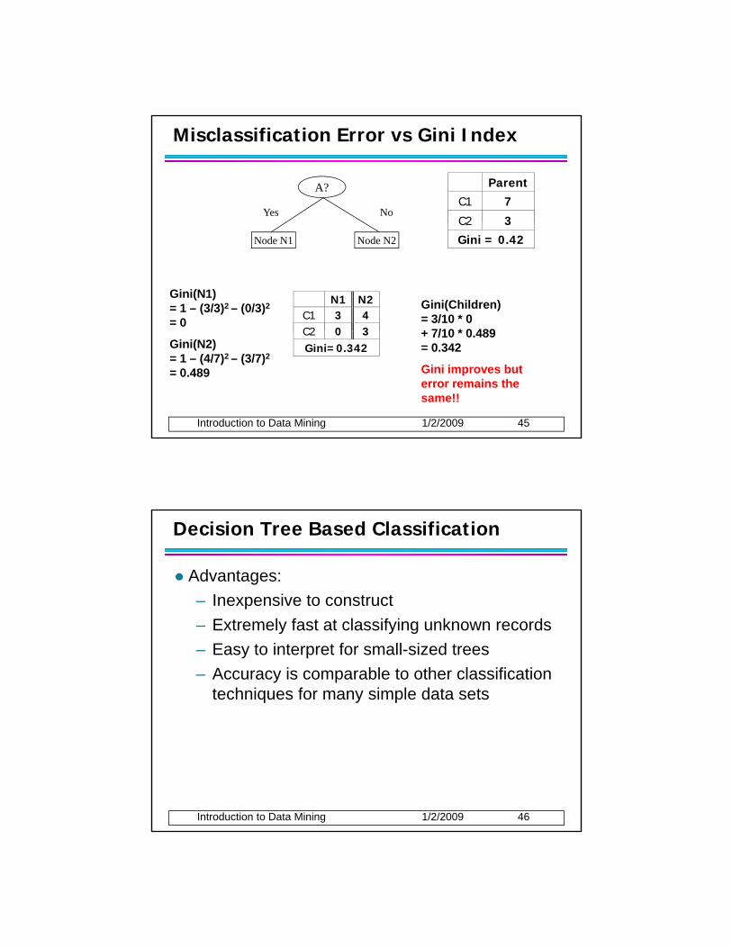
Misclassification Error vs Gini Index

A?

Yes No

Parent C1 7

C2 3

Node N1 Node N2

C2 3Gini = 0.42

N1 N2 C1 3 4 C2 0 3

Gini(N1) = 1 – (3/3)2 – (0/3)2

= 0 Gini(Children) = 3/10 * 0 + 7/10 * 0 489


C2 0 3Gini=0.342

Gini(N2) = 1 – (4/7)2 – (3/7)2

= 0.489

+ 7/10 * 0.489= 0.342

Gini improves but error remains the same!!

Decision Tree Based Classification

Advantages:– Inexpensive to construct– Extremely fast at classifying unknown records– Easy to interpret for small-sized trees– Accuracy is comparable to other classification

techniques for many simple data sets


Classification: Basic Concepts, Decision Trees, and Model...

Documents

Transcript of Classification: Basic Concepts, Decision Trees, and Model...